Closed-Loop Sparse Channel Estimation for Wideband Millimeter-Wave Full-Dimensional MIMO Systems

Abstract

This paper proposes a closed-loop sparse channel estimation (CE) scheme for wideband millimeter-wave hybrid full-dimensional multiple-input multiple-output and time division duplexing based systems, which exploits the channel sparsity in both angle and delay domains. At the downlink CE stage, random transmit precoding matrix is designed at base station (BS) for channel sounding, and receive combining matrices at user devices (UDs) are designed whereby the hybrid array is visualized as a low-dimensional digital array for facilitating the multi-dimensional unitary ESPRIT (MDU-ESPRIT) algorithm to estimate respective angle-of-arrivals (AoAs). At the uplink CE stage, the estimated downlink AoAs, namely, uplink angle-of-departures (AoDs), are exploited to design multi-beam transmit precoding matrices at UDs to enable BS to estimate the uplink AoAs, i.e., the downlink AoDs, and delays of different UDs, whereby the MDU-ESPRIT algorithm is used based on the designed receive combining matrix at BS. Furthermore, a maximum likelihood approach is proposed to pair the channel parameters acquired at the two stages, and the path gains are then obtained using least squares estimator. According to spectrum estimation theory, our solution can acquire the super-resolution estimations of the AoAs/AoDs and delays of sparse multipath components with low training overhead. Simulation results verify the better CE performance and lower computational complexity of our solution over state-of-the-art approaches.

I Introduction

Millimeter-wave (mmWave) communication with the aid of massive multiple-input multiple-output (MIMO) is an enabling technology for next-generation mobile communications, since the abundant spectrum resources at mmWave frequency band can boost the throughput by orders of magnitude [1, 2]. To mitigate the severe path loss for mmWave signal, massive MIMO is usually integrated into mmWave communications to form beams for directional signal transmission [3, 4]. However, the powerful fully-digital MIMO architecture, which requires a radio frequency (RF) chain for each antenna, is unaffordable for mmWave massive MIMO, due to the prohibitive hardware cost and power consumption of RF chains required [5]. The hybrid MIMO architecture with a much smaller number of RF chains than that of antennas offers a practical solution by using hybrid analog/digital beamforming [6]. Nonetheless, for such a hybrid MIMO system, it is challenging to estimate the high-dimensional mmWave channel from the low-dimensional effective measurements observed from the limited number of RF chains, since the training overhead for channel estimation (CE) can be excessively high [2]. Moreover, the low signal-to-noise ratio (SNR) before beamforming can further degrade the performance of channel state information (CSI) acquisition [7].

I-A Related Work

Several approaches were proposed in the literature to acquire CSI for narrowband mmWave communications, including codebook-based beam training [8, 9, 10, 11] and compressed sensing (CS)-based CE [12, 13]. The beam training approaches were initially adopted in analog beamforming, e.g., IEEE standards 802.11ad [8] and 802.15.3c [2], where the transceiver exhaustively searches for the optimal beam pair from a predefined codebook to maximize the received SNR for improved transmission performance. To reduce the search dimension of codebooks for achieving lower training overhead, the multi-stage overlapped beam patterns were designed in [9], where the beam patterns can become narrow as the training stage increases. However, these schemes only consider the analog beamforming with single-stream transmission. For hybrid beamforming with multi-stream transmission, beam training solutions with hierarchical multi-beam codebooks were proposed in [10, 11], where the optimal multi-beam pairs can be acquired after hierarchical beam search with gradually finer and narrower beams. However, the training overhead of a beam training scheme is usually proportional to the dimension of codebook, which is very large for full-dimensional (FD) MIMO with a large number of antennas. By exploiting the inherent angle-domain sparsity of mmWave MIMO channels, several CS-based CE schemes were proposed to reduce the CE overhead [12, 13]. In [12], the orthogonal matching pursuit (OMP) algorithm was considered to estimate sparse mmWave channels by formulating the CSI acquisition problem as a sparse signal recovery problem, where a redundant dictionary with non-uniformly quantized angle-domain girds was designed for improved performance. Furthermore, a Bayesian CS-based CE scheme was proposed in [13] by considering the impact of transceiver hardware impairments. Besides, by leveraging the low-rank property of mmWave channels, a CANDECOMP/PARAFAC decomposition-based CE scheme [14] was proposed with further improved performance.

The aforementioned solutions [9, 10, 11, 12, 13, 14] only consider frequency-flat mmWave channels but practical mmWave channels can be frequency selective due to the very large system bandwidth in mmWave frequency band and the distinct delay spreads of multipath components (MPCs) [15]. A distributed grid matching pursuit (DGMP) algorithm was proposed in [16] to estimate time-dispersive channels, where orthogonal frequency division multiplexing (OFDM) is considered. An adaptive grid matching pursuit (AGMP) algorithm developed from the DGMP was proposed to reduce power leakage by using adaptive grid matching solution [17]. In [18], the sparse mmWave channels at different subcarriers were estimated separately by utilizing the OMP, but the computational complexity is high as the number of subcarriers is typically large. To reduce complexity, a simultaneous weighted (SW)-OMP based scheme was proposed in [19], which exploits the angle-domain common sparsity of channels at different subcarriers to improve performance. By leveraging the common sparsity of delay-domain channels among transceiver antenna pairs, a block CS-based CE solution was proposed for mmWave fully-digital MIMO system [20], where the training sequences are designed to improve CE performance. Based on the low-rank property of wideband mmWave channels, the training signal received can be formulated as a high-order tensor with the low-rank CANDECOMP/PARAFAC decomposition to estimate the dominated channel parameters, including angle-of-arrivals/angle-of-departures (AoAs/AoDs) and delays [21]. However, most CS-based CE schemes for wideband mmWave MIMO usually adopt discrete AoAs/AoDs grids in CS dictionary, but the practical AoAs/AoDs of MPCs are continuously distributed. This mismatch may degrade CE performance. Moreover, the state-of-the-art works [9, 10, 11, 12, 13, 14, 16, 17, 20, 18, 19, 21, 22] usually focus on the ideal uniform linear array (ULA) while seldom investigate the practical uniform planar array (UPA). Compared to the ULA, the UPA offers more compact array with three-dimensional (3-D) beamforming in both horizontal and vertical directions [23, 24], leading to the FD-MIMO. Although mmWave FD-MIMO CE has been investigated in [23] and [24], they only considered either fully-digital MIMO or frequency-flat channels.

Figure 1: The air-ground mmWave channels between the UAV aerial-BS and UDs exhibit sparsity in both angle-domain and delay-domain due to the limited significant scatterers [25, 26].

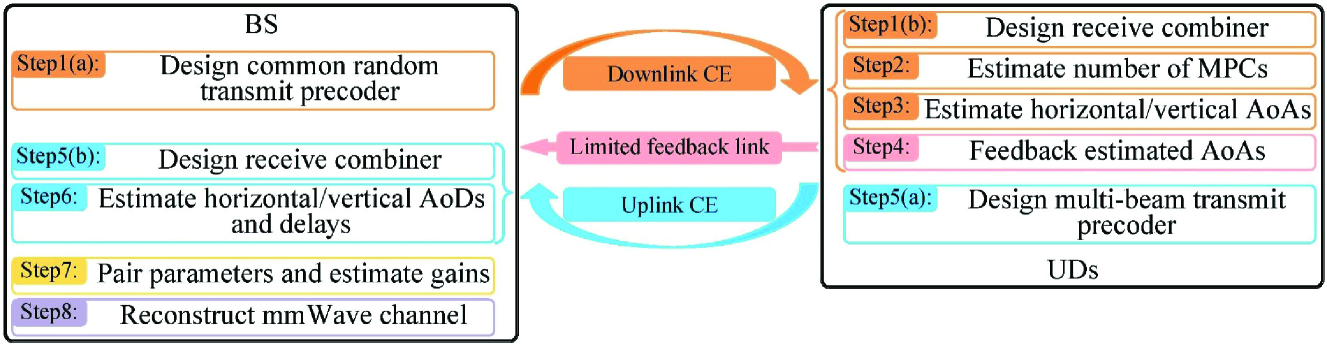
Figure 2: Procedure of the proposed closed-loop sparse CE solution, where the limited feedback is realized via the low-frequency control link.

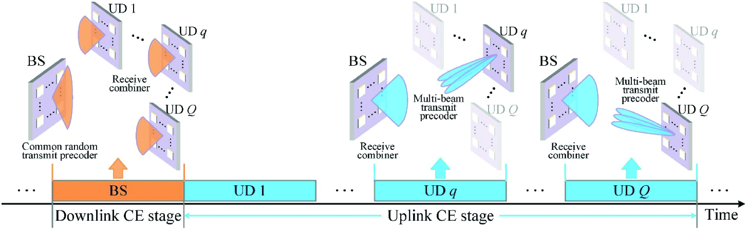
Figure 3: Frame structure of the proposed closed-loop sparse CE solution.

I-B Our Contributions

We propose a closed-loop sparse CE scheme for multi-user wideband mmWave FD-MIMO systems by exploiting the sparsity of MPCs in both angle and delay domains. To illustrate this sparsity, we consider the mmWave FD-MIMO based unmanned aerial vehicle (UAV) aerial-base station (BS), as shown in Fig. 1, which has flexible deployment capacity to serve user devices (UDs) in hotspot areas [27]. Different from the terrestrial BS in 3GPP or QuaDRiGa [28], [29], UAV aerial-BS usually works at the height of hundreds of meters, where fewer MPCs corresponding to dominant scatterers could establish the communications links between the aerial-BS and UD. Therefore, the air-ground mmWave channels in such aerial-BS based systems exhibit inherent sparsity in both angle and delay domains due to the limited significant scatterers. By carefully designing the transmit beamforming or precoding and receive combining in the training stage, our solution is capable of acquiring the super-resolution estimates of AoAs, AoDs, and delays based on spectrum estimation theory [30, 31] with low training overhead and computational complexity. In terms of sparse mmWave UAV air-ground channels, the proposed CE scheme can obtain a better performance of parametric CE. To clearly show the novelty and new contribution of our proposed solution as well as to contrast it with the existing solutions, below we conceptually explain our proposed closed-loop sparse CE scheme.

Our closed-loop solution includes the downlink CE stage followed by the uplink CE stage as illustrated in Fig. 2, where the channel reciprocity in time division duplex (TDD) based systems is exploited [32, 33, 34]. In TDD based systems, downlink AoAs (AoDs) are uplink AoDs (AoAs). The frame structure of our solution is further depicted in Fig. 3. As shown in Figs. 2 and 3, at the downlink CE stage, the horizontal/vertical AoAs of sparse MPCs are first estimated at each UD and they are fed back to the BS with limited quantization accuracy through the feedback link. At this stage, we design a common random transmit precoding matrix at the BS to transmit the training signals for omnidirectional channel sounding and we design the receive combining matrix at each UD to visualize the high-dimensional hybrid array as a low-dimensional digital array, which facilitates the use of the multi-dimensional unitary ESPRIT (MDU-ESPRIT) algorithm to estimate channel parameters. Similarly, at the uplink CE stage, the horizontal/vertical AoDs and delays associated with different UDs are successively estimated by using the MDU-ESPRIT algorithm at the BS. Owing to the channel reciprocity, the AoAs estimated at UD side can be utilized as a priori to design the multi-beam transmit precoding matrix to improve the received SNR for uplink CE. A maximum likelihood (ML) approach is adopted at the BS to pair the channel parameters acquired at these two stages and, consequently, the associated path gains can readily be obtained using the least squares (LS) estimator. Finally, the mmWave channel associated with each UD can be separately reconstructed based on the dominant channel parameters estimated above.

In contrast to the existing solutions, our main contributions are summarized as follows:

• We propose a closed-loop sparse CE solution with the common downlink CE stage for all UDs and the dedicated uplink CE stage for each UD. At the downlink CE stage, the BS fully exploits its large transmit power to allow multiple UDs simultaneously perform CE for reduced training overhead, and only horizontal/vertical AoAs estimation with low computational complexity is required at UDs. At the uplink CE stage, the multi-beam transmit precoding matrices are designed at UDs to enhance CE accuracy, and the BS with high computational capacity can jointly estimate horizontal/vertical AoDs and delays. By contrast, the state-of-the-art CS-based solutions [16, 17, 18, 19] are all based on open-loop approach, which imposes high computational complexity and storage requirements on the receiver. It is worth emphasizing that by exploiting the horizontal/vertical AoAs estimated at the downlink CE stage, the multi-beam transmit precoding matrices designed at UDs significantly improve received SNR, which works even for the case that the number of MPCs is larger than that of RF chains, i.e., the number of beams can be larger than that of RF chains.

• We design the receive combining matrices at UDs and BS for visualizing the hybrid array as a digital array, to enable the application of spectrum estimation techniques. For hybrid MIMO, it is challenging to directly apply spectrum estimation techniques to estimate channel parameters, since the shift-invariance structure of array response matrix observed from the digital baseband domain does not hold [31, 35]. Our solution sheds light on how to apply spectrum estimation techniques, e.g., ESPRIT-type algorithms, to hybrid MIMO, so that the super-resolution estimation of channel parameters can be acquired with low training overhead and computational complexity. By contrast, to achieve the high-resolution estimations of channel parameters, the existing CS-based solutions [16, 17, 18, 19] usually rely on the high-dimensional angle-domain or delay-domain redundant dictionary, which poses the excessively high computational complexity and storage requirements for FD-MIMO systems with large-scale antenna arrays.

• The double sparsity of MPCs in both angle and delay domains is harnessed in our proposed CE scheme. By leveraging the double sparsity, our scheme formulates the CE problem as a multi-dimensional spectrum estimation problem, where the super-resolution estimations of horizontal/vertical AoAs/AoDs and delays can be obtained simultaneously. By comparison, the existing CE solutions [16, 17, 19] only consider the angle-domain sparsity of mmWave channels. Moreover, the delay-domain CE approaches of [18, 20] have to estimate the effective delay-domain channel impulse response (CIR), which includes the time-domain pulse shaping filter (PSF) that can weaken the delay-domain channel sparsity. By contrast, the super-resolution estimation of delays in our solution is immune to PSF.

Throughout this paper, boldface lower and upper-case symbols denote column vectors and matrices, respectively. $(\cdot)^{*}$, $(\cdot)^{\rm T}$, $(\cdot)^{\rm H}$, $(\cdot)^{-1}$, $\left\lceil\cdot\right\rceil$ and $\left\lfloor\cdot\right\rfloor$ denote the conjugate, transpose, Hermitian transpose, matrix inversion, integer ceiling and integer floor operators, respectively. $\|\bm{a}\|_{1}$ and $\|\bm{a}\|_{2}$ are ${\ell_{1}}$-norm and ${\ell_{2}}$-norm of $\bm{a}$, respectively, while $\|\bm{A}\|_{F}$ is Frobenius norm of $\bm{A}$, and $|{\cal Q}|_{c}$ is the cardinality of the set ${\cal Q}$. The Kronecker and Khatri-Rao product operations are denoted by $\otimes$ and $\odot$, respectively. $\bm{I}_{n}$ denotes the $n\times n$ identity matrix and $\bm{O}_{m\times n}$ is the null matrix of size $m\times n$, while $\bm{1}_{n}$ ($\bm{0}_{n}$) denotes the vector of size $n$ with all the elements being $1$ ($0$). $\text{diag}(\bm{a})$ is the diagonal matrix with the elements of $\bm{a}$ at its diagonal entries, $\text{vdiag}(\bm{A})$ denotes the vector consisting of the main diagonal elements of $\bm{A}$, and $\text{Bdiag}([\bm{A}_{1}\cdots\bm{A}_{n}])$ denotes the block diagonal matrix with $\bm{A}_{1},\cdots,\bm{A}_{n}$ as its block diagonal entries. The expectation and determinant operators are denoted by $\mathbb{E}(\cdot)$ and $\det(\cdot)$, respectively. The modulo operation $\text{mod}(m,n)$ returns the remainder of dividing $m$ by $n$, and $\text{mod}({\cal Q},n)$ returns the set containing $\text{mod}(m,n)$ $\forall m\in{\cal Q}$ of the ordered set ${\cal Q}$. The operator $\text{find}(\bm{a}\neq 0)$ returns the set containing the indices of nonzero elements of $\bm{a}$, and $\text{mat}(\bm{a};m,n)$ converts the vector $\bm{a}$ of size $mn$ into the matrix of size $m\times n$ by successively selecting every $m$ elements of $\bm{a}$ as its columns. The operator $\text{vec}(\bm{A})$ stacks the columns of ${\bm{A}}$ on top of each another, $[\bm{A}]_{m,n}$ denotes the $m$th-row and $n$th-column element of $\bm{A}$, and $\bm{a}_{[m:n]}$ is the vector consisting the $m$th to $n$th elements of $\bm{a}$, while $\bm{A}_{[:,m:n]}$ is the sub-matrix containing the $m$th to $n$th columns of $\bm{A}$. $\bm{A}_{[{\cal Q},:]}$ denotes the sub-matrix containing the rows of $\bm{A}$ indexed in the ordered set ${\cal Q}$, and $\bm{A}_{[{\cal Q},i]}$ is the $i$th column of $\bm{A}_{[{\cal Q},:]}$. Finally, $\Re\{\cdot\}$ and $\Im\{\cdot\}$ denote the real part and imaginary part of the argument, respectively.

II Downlink Channel Estimation Stage

Consider the mmWave FD-MIMO system with hybrid beamforming, where the BS and $Q$ UDs are all equipped with UPA, and OFDM with $K$ subcarriers is adopted, while $N_{\rm s}^{d}$ independent signal streams are transmitted on each subcarrier [16]. The BS (UD) employs $N_{\rm BS}=N_{\rm BS}^{\rm h}N_{\rm BS}^{\rm v}$ ($N_{\rm UD}=N_{\rm UD}^{\rm h}N_{\rm UD}^{\rm v}$) antennas and $N_{\rm BS}^{\rm RF}\ll N_{\rm BS}$ ($N_{\rm UD}^{\rm RF}\ll N_{\rm UD}$) RF chains, where $N_{\rm BS}^{\rm h}$ ($N_{\rm UD}^{\rm h}$) and $N_{\rm BS}^{\rm v}$ ($N_{\rm UD}^{\rm v}$) are the numbers of antennas in horizontal and vertical directions at the BS (UD), respectively.

II-A Downlink Channel Estimation Signal Model

The downlink CE stage lasts $N_{d}$ time slots and each time slot contains $N_{\rm o}^{d}$ OFDM symbols. The signal $\bm{y}_{q}[k,i,m]\!\in\!\mathbb{C}^{N_{\rm s}^{d}}$ received by the $q$th UD at the $k$th subcarrier of the $i$th OFDM symbol in the $m$th time slot can be expressed as

$$\begin{split}\bm{y}_{q}[k,i,m]=&\bm{W}_{d,q}^{\rm H}[k,m]\bm{H}_{q}[k]\bm{F}_{d}[k,m]\bm{s}[k,i,m]\\ \ &+\bm{W}_{d,q}^{\rm H}[k,m]\bm{n}_{q}[k,i,m],\end{split}$$ (1)

for $1\!\leq\!q\!\leq\!Q$, $0\!\leq\!k\!\leq\!K-1$, $1\!\leq\!i\!\leq\!N_{\rm o}^{d}$ and $1\!\leq\!m\!\leq\!N_{d}$. In (1), the UD’s receive combining matrix $\bm{W}_{d,q}[k,m]\!=\!\bm{W}_{{\rm RF},q}[m]\bm{W}_{{\rm BB},q}[k,m]\!\in\!\mathbb{C}^{N_{\rm UD}\times N_{\rm s}^{d}}$ in which $\bm{W}_{{\rm RF},q}[m]\!\in\!\mathbb{C}^{N_{\rm UD}\times N_{\rm UD}^{\rm RF}}$ and $\bm{W}_{{\rm BB},q}[k,m]\!\in\!\mathbb{C}^{N_{\rm UD}^{\rm RF}\times N_{\rm s}^{d}}$ are the analog and digital receive combining matrices, and the BS’s transmit precoding matrix $\bm{F}_{d}[k,m]\!=\!\bm{F}_{{\rm RF},d}[m]\bm{F}_{{\rm BB},d}[k,m]\!\in\!\mathbb{C}^{N_{\rm BS}\times N_{\rm s}^{d}}$ in which $\bm{F}_{{\rm RF},d}[m]\!\in\!\mathbb{C}^{N_{\rm BS}\times N_{\rm BS}^{\rm RF}}$ and $\bm{F}_{{\rm BB},d}[k,m]\!\in\!\mathbb{C}^{N_{\rm BS}^{\rm RF}\times N_{\rm s}^{d}}$ are the analog and digital transmit precoding matrices, respectively, while $\bm{H}_{q}[k]\!\in\!\mathbb{C}^{N_{\rm UD}\times N_{\rm BS}}$ is the corresponding downlink channel matrix, $\bm{s}[k,i,m]\!\in\!\mathbb{C}^{N_{\rm s}^{d}}$ is the training signal with $\mathbb{E}\left(\bm{s}[k,i,m]\bm{s}^{\rm H}[k,i,m]\right)\!=\!\frac{1}{N_{\rm s}^{d}}\bm{I}_{N_{\rm s}^{d}}$, and $\bm{n}_{q}[k,i,m]\!\in\!\mathbb{C}^{N_{\rm UD}}$ is the complex additive white Gaussian noise (AWGN) vector with the covariance matrix $\sigma_{n}^{2}\bm{I}_{N_{\rm UD}}$, i.e., $\bm{n}_{q}[k,i,m]\!\sim\!{\cal CN}\!\left(\bm{0}_{N_{\rm UD}},\sigma_{n}^{2}\bm{I}_{N_{\rm UD}}\right)$. Due to the constant modulus of the phase shift network (PSN), $\left[\bm{F}_{{\rm RF},d}[m]\right]_{j_{1},j_{2}}\!=\!\frac{1}{\sqrt{N_{\rm BS}}}e^{\textsf{j}\vartheta_{1,j_{1},j_{2}}}$ and $\left[\bm{W}_{{\rm RF},q}[m]\right]_{j_{1},j_{2}}\!=\!\frac{1}{\sqrt{N_{\rm UD}}}e^{\textsf{j}\vartheta_{2,j_{1},j_{2}}}$ with $\vartheta_{1,j_{1},j_{2}},\vartheta_{2,j_{1},j_{2}}\!\in\!{\cal A}$, and ${\cal A}$ is the quantized phase set of the PSN with the resolution $N_{q}^{\rm ps}$, given by

$${\cal A}= \left\{-\pi,-\pi+{\textstyle{2\pi\over 2^{N_{q}^{\rm ps}}}},-\pi+2\cdot{\textstyle{2\pi\over 2^{N_{q}^{\rm ps}}}},\cdots,\pi-{\textstyle{2\pi\over 2^{N_{q}^{\rm ps}}}}\right\}.$$ (2)

Also $\left\|\bm{F}_{d}[k,m]\right\|_{F}^{2}\leq N_{\rm BS}^{\rm RF}$ to guarantee the constraint on the total transmit power [5]. Here at the CE stage, some elegant solutions [39, 42] can be used to acquire the robust synchronization of burst training signals without the knowledge of noise/interference power even at low SNR.

Due to the obviously resolvable delay spread for each MPC caused by the large bandwidth, according to the typical mmWave channel model [21, 16, 17, 18, 19, 20, 25], the downlink delay-domain continuous channel matrix $\bm{H}_{q}(\tau)\in\mathbb{C}^{N_{\rm UD}\times N_{\rm BS}}$ with $L_{q}$ MPCs can be expressed as

$$\bm{H}_{q}(\tau)= \beta_{q}\sum\limits_{l=1}^{L_{q}}\bm{H}_{q,l}p\left(\tau-\tau_{q,l}\right),$$ (3)

where $\beta_{q}=\sqrt{N_{\rm UD}N_{\rm BS}/L_{q}}$ is the normalization factor, $\tau_{q,l}$ is the delay of the $l$th MPC, and $p(\tau)$ denotes the equivalent PSF, while the complex gain matrix $\bm{H}_{q,l}\in\mathbb{C}^{N_{\rm UD}\times N_{\rm BS}}$ is given by

$$\bm{H}_{q,l}=\alpha_{q,l}\bm{a}_{\rm UD}\left(\mu_{q,l}^{\rm UD},\nu_{q,l}^{\rm UD}\right)\bm{a}_{\rm BS}^{\rm H}\left(\mu_{q,l}^{\rm BS},\nu_{q,l}^{\rm BS}\right),$$ (4)

where $\alpha_{q,l}\!\sim\!{\cal CN}(0,\sigma_{\alpha}^{2})$ is the associated complex path gain, $\mu_{q,l}^{\rm UD}\!=\!\pi\sin\big{(}\theta_{q,l}^{\rm UD}\big{)}\cos\big{(}\varphi_{q,l}^{\rm UD}\big{)}$ ($\mu_{q,l}^{\rm BS}\!=\!\pi\sin\big{(}\theta_{q,l}^{\rm BS}\big{)}\cos\big{(}\varphi_{q,l}^{\rm BS}\big{)}$) and $\nu_{q,l}^{\rm UD}\!=\!\pi\sin\big{(}\varphi_{q,l}^{\rm UD}\big{)}$ ($\nu_{q,l}^{\rm BS}\!=\!\pi\sin\big{(}\varphi_{q,l}^{\rm BS}\big{)}$) denote the horizontally and vertically spatial frequencies with half-wavelength antenna spacing at the $q$th UD (the BS), respectively. Here, $\theta_{q,l}^{\rm UD}$ ($\theta_{q,l}^{\rm BS}$) and $\varphi_{q,l}^{\rm UD}$ ($\varphi_{q,l}^{\rm BS}$) are the downlink horizontal and vertical AoAs (AoDs) of the $l$th MPC associated with the UPA, respectively. The array response vector at UD is given by $\bm{a}_{\rm UD}\big{(}\mu_{q,l}^{\rm UD},\nu_{q,l}^{\rm UD}\big{)}=\bm{a}_{\rm v}\big{(}\nu_{q,l}^{\rm UD}\big{)}\otimes\bm{a}_{\rm h}\big{(}\mu_{q,l}^{\rm UD}\big{)}\in\mathbb{C}^{N_{\rm UD}}$ [24, 30, 36], in which

$$\bm{a}_{\rm h}\left(\mu_{q,l}^{\rm UD}\right)= {\textstyle{1\over{\sqrt{N_{\rm UD}^{\rm h}}}}}\big{[}1~{}e^{\textsf{j}\mu_{q,l}^{\rm UD}}\cdots e^{\textsf{j}\left(N_{\rm UD}^{\rm h}-1\right)\mu_{q,l}^{\rm UD}}\big{]}^{\rm T},$$ (5)

$$\bm{a}_{\rm v}\left(\nu_{q,l}^{\rm UD}\right)= {\textstyle{1\over{\sqrt{N_{\rm UD}^{\rm v}}}}}\big{[}1~{}e^{\textsf{j}\nu_{q,l}^{\rm UD}}\cdots e^{\textsf{j}\left(N_{\rm UD}^{\rm v}-1\right)\nu_{q,l}^{\rm UD}}\big{]}^{\rm T}.$$ (6)

are the steering vectors associated with the horizontal and vertical directions, respectively. Similarly, the array response vector at BS is given by $\bm{a}_{\rm BS}\big{(}\mu_{q,l}^{\rm BS},\nu_{q,l}^{\rm BS}\big{)}=\bm{a}_{\rm v}\big{(}\nu_{q,l}^{\rm BS}\big{)}\otimes\bm{a}_{\rm h}\big{(}\mu_{q,l}^{\rm BS}\big{)}\in\mathbb{C}^{N_{\rm BS}}$, where the horizontal and vertical direction steering vectors $\bm{a}_{\rm h}\big{(}\mu_{q,l}^{\rm BS}\big{)}\in\mathbb{C}^{N_{\rm BS}^{\rm h}}$ and $\bm{a}_{\rm h}\big{(}\nu_{q,l}^{\rm BS}\big{)}\in\mathbb{C}^{N_{\rm BS}^{\rm v}}$ are given respectively by substituting $\mu_{q,l}^{\rm UD}$ and $N_{\rm UD}^{\rm h}$ with $\mu_{q,l}^{\rm BS}$ and $N_{\rm BS}^{\rm h}$ in (5) as well as by substituting $\nu_{q,l}^{\rm UD}$ and $N_{\rm UD}^{\rm v}$ with $\nu_{q,l}^{\rm BS}$ and $N_{\rm BS}^{\rm v}$ in (6).

The frequency-domain channel matrix $\bm{H}_{q}[k]$ at the $k$th subcarrier can then be expressed as

$$\begin{split}\bm{H}_{q}[k]&=\beta_{q}\sum\limits_{l=1}^{L_{q}}\bm{H}_{q,l}e^{-\textsf{j}\frac{2\pi kf_{s}\tau_{q,l}}{K}}\\[-2.84526pt] =\beta_{q}&\sum\limits_{l=1}^{L_{q}}\alpha_{q,l}\bm{a}_{\rm UD}\left(\mu_{q,l}^{\rm UD},\nu_{q,l}^{\rm UD}\right)\bm{a}_{\rm BS}^{\rm H}\left(\mu_{q,l}^{\rm BS},\nu_{q,l}^{\rm BS}\right)e^{-\textsf{j}\frac{2\pi kf_{s}\tau_{q,l}}{K}},\end{split}$$ (7)

where $f_{s}=1/T_{s}$ denotes the system bandwidth, and $T_{s}$ is the sampling period. The derivation of the first equation in (7) is shown in Appendix. Observe that $\bm{H}_{q}[k]$ does not depend on the PSF, and it exhibits the sparsity in delay domain due to small $L_{q}$ but large normalized delay spread. Recall that the existing CS-based solutions of [18, 20] have to estimate the effective delay-domain CIRs that include the PSF, and this PSF will destroy the delay-domain sparsity of mmWave channels when the order of PSF is large. $\bm{H}_{q}[k]$ in (7) can be rewritten as

$$\bm{H}_{q}[k]=\bm{A}_{{\rm UD},q}\bm{D}_{q}[k]\bm{A}_{{\rm BS},q}^{\rm H},$$ (8)

where $\bm{D}_{q}[k]\!=\!\text{diag}\left(\bm{d}_{q}[k]\right)\!\in\!\mathbb{C}^{L_{q}\times L_{q}}$ is the diagonal matrix in which $\bm{d}_{q}[k]\!=\!\text{diag}\left(\bm{\alpha}_{q}\right)\bm{\tau}_{q}[k]$ with $\bm{\alpha}_{q}\!=\!\beta_{q}\left[\alpha_{q,1}\cdots\alpha_{q,L_{q}}\right]^{\rm T}$ and $\bm{\tau}_{q}[k]\!=\!\big{[}e^{-\textsf{j}2\pi kf_{s}\tau_{q,1}/K}\cdots e^{-\textsf{j}2\pi kf_{s}\tau_{q,L_{q}}/K}\big{]}^{\rm T}$, and the array response matrix associated with the AoAs of the $q$th UD $\bm{A}_{{\rm UD},q}\!\in\!\mathbb{C}^{N_{\rm UD}\times L_{q}}$ can be expressed as $\bm{A}_{{\rm UD},q}\!=\!\bm{A}_{{\rm UD},q}^{\nu}\!\odot\!\bm{A}_{{\rm UD},q}^{\mu}$ in which $\bm{A}_{{\rm UD},q}^{\mu}\!=\!\big{[}\bm{a}_{\rm h}(\mu_{q,1}^{\rm UD})\cdots\bm{a}_{\rm h}(\mu_{q,L_{q}}^{\rm UD})\big{]}\!\in\!\mathbb{C}^{N_{\rm UD}^{\rm h}\times L_{q}}$ and $\bm{A}_{{\rm UD},q}^{\nu}\!=\!\big{[}\bm{a}_{\rm v}(\nu_{q,1}^{\rm UD})\cdots\bm{a}_{\rm v}(\nu_{q,L_{q}}^{\rm UD})\big{]}\!\in\!\mathbb{C}^{N_{\rm UD}^{\rm v}\times L_{q}}$ are the steering matrices corresponding to the horizontally and vertically spatial frequencies, respectively, while $\bm{A}_{{\rm BS},q}\!=\!\bm{A}_{{\rm BS},q}^{\nu}\!\odot\!\bm{A}_{{\rm BS},q}^{\mu}\!\in\!\mathbb{C}^{N_{\rm BS}\times L_{q}}$ is the array response matrix associated with the AoDs in which the steering matrices $\bm{A}_{{\rm BS},q}^{\mu}\!\in\!\mathbb{C}^{N_{\rm BS}^{\rm h}\times L_{q}}$ and $\bm{A}_{{\rm BS},q}^{\nu}\!\in\!\mathbb{C}^{N_{\rm BS}^{\rm v}\times L_{q}}$ have the similar form as $\bm{A}_{{\rm UD},q}^{\mu}$ and $\bm{A}_{{\rm UD},q}^{\nu}$, respectively.

II-B Obtain Horizontal/Vertical AoAs at UD

The downlink CE corresponds to Step 1 to Step 4 of Fig. 2, where the horizontal and vertical AoAs are estimated. We first assume that the training signal $\bm{s}[i,m]$ is independent of subcarriers, and its $j_{1}$th element can be designed as $\left[\bm{s}[i,m]\right]_{j_{1}}\!=\!\frac{1}{N_{\rm s}^{d}}e^{\textsf{j}2\pi\phi_{j_{1}}}$ with $\phi_{j_{1}}$ randomly and uniformly selected from the interval $[0,\,1]$, i.e., $\phi_{j_{1}}\sim{\cal U}[0,~{}1]$. Second, a predefined frequency-domain scrambling code $\bm{x}_{d}\in\mathbb{C}^{K}$ with its $k$th element being $x_{d}[k]$ for $0\!\leq\!k\!\leq\!K-1$ can be introduced to effectively avoid the high peak-to-average power ratio (PAPR) resulted from the same training signal used at all subcarriers. Then, we can obtain the scrambled training signal $\bm{s}[k,i,m]$ at the $k$th subcarrier, i.e., $\bm{s}[k,i,m]\!=\!x_{d}[k]\bm{s}[i,m]$. The signals received at the UD will be first descrambled by multiplying the conjugate of scrambling code $\bm{x}_{d}^{*}$, which indicates that the scrambling code $\bm{x}_{d}$ does not affect the subsequent signal processing. Moreover, the same digital transmit precoding/receive combining matrices are adopted at every subcarrier, i.e., $\bm{F}_{{\rm BB},d}[k,m]\!=\!\bm{F}_{{\rm BB},d}[m]$ and $\bm{W}_{{\rm BB},q}[k,m]\!=\!\bm{W}_{{\rm BB},q}[m]$, for $0\!\leq\!k\!\leq\!K-1$. The number of independent signal streams associated with each subcarrier in each OFDM symbol is $N_{\rm s}^{d}\!\leq\!N_{\rm UD}^{\rm RF}$. We can visualize a low-dimensional digital $M_{\rm UD}^{\rm h}\!\times\!M_{\rm UD}^{\rm v}$ sub-UPA, in which $M_{\rm UD}^{\rm h}$ and $M_{\rm UD}^{\rm v}$ are the numbers of antennas in horizontal and vertical directions, from the high-dimensional hybrid analog/digital ${N_{\rm UD}^{\rm{h}}}\times{N_{\rm UD}^{\rm{v}}}$ UPA. Given $N_{\rm UD}^{\rm sub}\!=\!M_{\rm UD}^{\rm h}M_{\rm UD}^{\rm v}$, the BS only requires $N_{d}\!=\!\left\lceil N_{\rm UD}^{\rm sub}/N_{\rm s}^{d}\right\rceil$ time slots to broadcast training signals, with each time slot containing $N_{\rm o}^{d}$ OFDM symbols. The choice of $M_{\rm UD}^{\rm h}$, $M_{\rm UD}^{\rm v}$ and $N_{\rm o}^{d}$ trades off estimation accuracy with training overhead, because larger $M_{\rm UD}^{\rm h}$, $M_{\rm UD}^{\rm v}$ and $N_{\rm o}^{d}$ lead to better estimation accuracy but higher training overhead, and vice versa. Since the signals received by all UDs have the same form, we can focus on the $q$th UD and the user index $q$ can be omitted from $\bm{y}_{q}[k,i,m]$, $\bm{W}_{d,q}[m]$, $\bm{H}_{q}[k]$, $\bm{n}_{q}[k,i,m]$, $\bm{A}_{{\rm UD},q}$, $\bm{D}_{q}[k]$, $\bm{A}_{{\rm BS},q}$ and other relevant variables for clarity.

By collecting the received signals of (1) associated with the $k$th subcarrier over all the $N_{\rm o}^{d}$ OFDM symbols of the $m$th time slot into the signal matrix $\bm{Y}_{m}[k]\!=\!\left[\bm{y}[k,1,m]\cdots\bm{y}[k,N_{\rm o}^{d},m]\right]\in\mathbb{C}^{N_{\rm s}^{d}\times N_{\rm o}^{d}}$, we have

$$\bm{Y}_{m}[k]\!=\!x_{d}^{*}[k]\bm{W}_{d}^{\rm H}[m]\bm{H}[k]\bm{F}_{d}[m]\bm{S}_{d}[k,m]\!+\!\bm{W}_{d}^{\rm H}[m]\bm{N}_{m}[k],$$ (9)

where $\bm{S}_{d}[k,m]\!=\!\left[\bm{s}[k,1,m]\cdots\bm{s}[k,N_{\rm o}^{d},m]\right]\!=\!x_{d}[k]\bm{S}_{d}[m]$ with $\bm{S}_{d}[m]\!=\!\left[\bm{s}[1,m]\cdots\bm{s}[N_{\rm o}^{d},m]\right]\!\in\!\mathbb{C}^{N_{\rm s}^{d}\times N_{\rm o}^{d}}$, and $\bm{N}_{m}[k]\!=\!\left[\bm{n}[k,1,m]\cdots\bm{n}[k,N_{\rm o}^{d},m]\right]\!\in\!\mathbb{C}^{N_{\rm UD}\times N_{\rm o}^{d}}$. Since the BS transmits the common random signal $\bm{F}_{d}[m]\bm{S}_{d}[m]$, the transmit precoding matrix $\bm{F}_{d}[m]\!=\!\bm{F}_{{\rm RF},d}[m]\bm{F}_{{\rm BB},d}[m]$ should be a random matrix. This is achieved by designing $\bm{F}_{{\rm RF},d}[m]$ as $\left[\bm{F}_{{\rm RF},d}[m]\right]_{j_{1},j_{2}}\!\!=\!\frac{1}{\sqrt{N_{\rm BS}}}e^{\textsf{j}\vartheta_{3,j_{1},j_{2}}}$ with ${\vartheta_{3,j_{1},j_{2}}}$ randomly and uniformly selected from ${\cal A}$, and designing $\bm{F}_{{\rm BB},d}[m]$ as $\left[\bm{F}_{{\rm BB},d}[m]\right]_{j_{1},j_{2}}\!\!=\!e^{\textsf{j}2\pi a_{j_{1},j_{2}}}$ with $a_{j_{1},j_{2}}\!\sim\!{\cal U}\left[0,1\right]$. The BS can use the same transmit precoding matrix $\bm{F}_{d}\!=\!\bm{F}_{d}[m]$ to send the same sounding signal $\bm{S}_{d}\!=\!\bm{S}_{d}[m]$ for every time slot. By stacking the received signal matrices $\bm{Y}_{m}[k]$ of (9) over the $N_{d}$ time slots into $\widetilde{\bm{Y}}_{d}[k]\!=\!\left[\bm{Y}_{1}^{\rm T}[k]\cdots\bm{Y}_{N_{d}}^{\rm T}[k]\right]^{\rm T}\!\in\!\mathbb{C}^{N_{d}N_{\rm s}^{d}\times N_{\rm o}^{d}}$, we have

$$\widetilde{\bm{Y}}_{d}[k]\!=\!\widetilde{\bm{W}}_{d}^{\rm H}\bm{A}_{\rm UD}\bm{D}[k]\bm{A}_{\rm BS}^{\rm H}\bm{F}_{d}\bm{S}_{d}\!+\!\text{Bdiag}\left(\check{\bm{W}}_{d}\right)\widetilde{\bm{N}}_{d}[k],$$ (10)

where $\widetilde{\bm{W}}_{d}\!=\!\left[\bm{W}_{d}[1]\cdots\bm{W}_{d}[N_{d}]\right]\!\in\!\mathbb{C}^{N_{\rm UD}\times N_{d}N_{\rm s}^{d}}$ aggregates the downlink receive combining matrices used in the $N_{d}$ time slots, and $\text{Bdiag}\left(\check{\bm{W}}_{d}\right)\!=\!\text{Bdiag}\left(\left[\bm{W}_{d}^{\rm H}[1]\cdots\bm{W}_{d}^{\rm H}[N_{d}]\right]\right)\!\in\!\mathbb{C}^{N_{d}N_{\rm s}^{d}\times N_{d}N_{\rm UD}}$, while $\widetilde{\bm{N}}_{d}[k]\!=\!\left[\bm{N}_{1}^{\rm T}[k]\cdots\bm{N}_{N_{d}}^{\rm T}[k]\right]^{\rm T}\!\in\!\mathbb{C}^{N_{d}N_{\rm UD}\times N_{\rm o}^{d}}$ is the corresponding noise matrix.

Multiplying $\widetilde{\bm{Y}}_{d}[k]$ with $\bm{J}_{d}\!=\!\big{[}\bm{I}_{N_{\rm UD}^{\rm sub}}\,\bm{O}_{N_{\rm UD}^{\rm sub}\times\left(N_{d}N_{\rm s}^{d}-N_{\rm UD}^{\rm sub}\right)}\big{]}$ and aggregating the resulting signals over all the $K$ subcarriers lead to the signal matrix $\bar{\bm{Y}}_{d}\!=\!\big{[}\bm{J}_{d}\widetilde{\bm{Y}}_{d}[0]~{}\bm{J}_{d}\widetilde{\bm{Y}}_{d}[1]\cdots\bm{J}_{d}\widetilde{\bm{Y}}_{d}[K-1]\big{]}\!\in\!\mathbb{C}^{N_{\rm UD}^{\rm sub}\times KN_{\rm o}^{d}}$ as

$$\bar{\bm{Y}}_{d}=\bar{\bm{A}}_{\rm UD}\bar{\bm{S}}_{d}+\bar{\bm{N}}_{d},$$ (11)

where $\bar{\bm{N}}_{d}\!=\!\bm{J}_{d}\text{Bdiag}\left(\check{\bm{W}}_{d}\right)\big{[}\widetilde{\bm{N}}_{d}[0]~{}\widetilde{\bm{N}}_{d}[1]\cdots\widetilde{\bm{N}}_{d}[K-1]\big{]}$, $\bar{\bm{A}}_{\rm UD}\!=\!\bm{J}_{d}\widetilde{\bm{W}}_{d}^{\rm H}\bm{A}_{\rm UD}$, and $\bar{\bm{S}}_{d}\!=\!\left[\bar{\bm{S}}_{d}[0]~{}\bar{\bm{S}}_{d}[1]\cdots\bar{\bm{S}}_{d}[K-1]\right]$ with $\bar{\bm{S}}_{d}[k]\!=\!\bm{D}[k]\bm{A}_{\rm BS}^{\rm H}\bm{F}_{d}\bm{S}_{d}$. Observe from (10) and (11) that we cannot directly apply powerful spectrum estimation techniques [30, 37] to estimate the horizontal/vertical AoAs from $\bar{\bm{Y}}_{d}$, since the shift-invariance structure of the array response matrix $\bm{A}_{\rm UD}$ does not hold in hybrid receive array [31, 35]. We propose to visualize the high-dimensional hybrid array as a low-dimensional digital array by designing appropriate aggregated receive combining matrix $\widetilde{\bm{W}}_{d}$ so that the shift-invariance structure of array response can be reconstructed and therefore super-resolution CE based on spectrum estimation techniques can be harnessed.

II-C Design Receive Combining Matrix at UD

Without loss of generality, we consider $N_{\rm s}^{d}\!=\!N_{\rm UD}^{\rm RF}\!-\!1$ independent signal streams. First, we utilize a unitary matrix $\bm{U}_{N_{\rm UD}^{\rm RF}}\!=\!\big{[}\bm{u}_{1}\cdots\bm{u}_{N_{\rm UD}^{\rm RF}}\big{]}\!\in\!\mathbb{C}^{N_{\rm UD}^{\rm RF}\times N_{\rm UD}^{\rm RF}}$ to design the digital receive combining matrix $\bm{W}_{\rm BB}[m]\!\in\!\mathbb{C}^{N_{\rm UD}^{\rm RF}\times N_{\rm s}^{d}}$ of the $m$th time slot’s receive combining matrix $\bm{W}_{d}[m]\!=\!\bm{W}_{\rm RF}[m]\bm{W}_{\rm BB}[m]$ for $1\!\leq\!m\!\leq\!N_{d}$. Specifically, $\bm{W}_{\rm BB}[m]\!=\!\bm{U}_{N_{\rm UD}^{\rm RF}[:,1:N_{\rm s}^{d}]}$. To design the analog receive combining matrix $\bm{W}_{\rm RF}[m]\!\in\!\mathbb{C}^{N_{\rm UD}\times N_{\rm UD}^{\rm RF}}$, we construct the matrix $\bm{\varXi}_{d}\!\in\!\mathbb{R}^{N_{\rm UD}\times N_{d}N_{\rm s}^{d}}$ as

$$\begin{split}\bm{\varXi}_{d}&=\left[\!\!\begin{array}[]{c}\bm{I}_{M_{\rm UD}^{\rm v}+1}\otimes\bm{B}\\ \bm{O}_{\left(N_{\rm UD}-N_{\rm UD}^{\rm h}\left(M_{\rm UD}^{\rm v}+1\right)\right)\times M_{\rm UD}^{\rm h}\left(M_{\rm UD}^{\rm v}+1\right)}\end{array}\right]\\ &\quad\times\left[\!\!\begin{array}[]{c}\bm{I}_{N_{\rm s}^{d}N_{d}}\\ \bm{O}_{\left(M_{\rm UD}^{\rm h}\left(M_{\rm UD}^{\rm v}+1\right)-N_{\rm s}^{d}N_{d}\right)\times N_{\rm s}^{d}N_{d}}\end{array}\right],\end{split}$$ (12)

where $\bm{B}\!=\!\big{[}\bm{I}_{M_{\rm UD}^{\rm h}}\,\bm{O}_{M_{\rm UD}^{\rm h}\times(N_{\rm UD}^{\rm h}-M_{\rm UD}^{\rm h})}\big{]}^{\rm T}\!\in\!\mathbb{R}^{N_{\rm UD}^{\rm h}\times M_{\rm UD}^{\rm h}}$. Then we take the sub-matrix $\bm{\varXi}_{d,m}^{\rm sub}\!=\!\bm{\varXi}_{d\,\left[:,(m-1)N_{\rm s}^{d}+1:mN_{\rm s}^{d}\right]}\!\in\!\mathbb{R}^{N_{\rm UD}\times N_{\rm s}^{d}}$ and define $\bar{\bm{\xi}}_{d,m}\!=\!\text{vec}({\bm{\varXi}_{d,m}^{\rm sub}})$ to construct the ordered index set ${\cal D}_{m}\!=\!{\rm find}\left(\bar{\bm{\xi}}_{d,m}\!\neq\!0\right)$ with $|{\cal D}_{m}|_{c}=N_{\rm s}^{d}$. Next we perform the modulo operation on ${\cal D}_{m}$ with $N_{\rm UD}$ to get the ordered index set ${\cal I}_{m}\!=\!\text{mod}({\cal D}_{m},N_{\rm UD})$ with $|{\cal I}_{m}|_{c}=N_{\rm s}^{d}$. The rows of $\bm{W}_{\rm RF}[m]$ whose indices correspond to ${\cal I}_{m}$ are determined by $\bm{W}_{\rm BB}[m]$ as $\bm{W}_{\rm RF}[m]_{[{\cal I}_{m},:]}\!=\!\bm{W}_{\rm BB}^{\rm H}[m]$, while the rest rows of $\bm{W}_{\rm RF}[m]$ consist of the $(N_{\rm UD}\!-\!N_{\rm s}^{d})$ identical $\bm{u}_{N_{\rm UD}^{\rm RF}}^{\rm H}$. The phase value of arbitrary element in the designed $\bm{W}_{\rm RF}[m]$, denoted by $\vartheta_{d}$, is then quantized to $\vartheta\!\in\!{\cal A}$ by minimizing the Euclidean distance according to $\arg\min\nolimits_{\vartheta\in{\cal A}}\!\left\|\vartheta_{d}\!-\!\vartheta\right\|_{2}$. Thus, the $m$th receive combining matrix can be obtained as $\bm{W}_{d}[m]\!=\!\bm{W}_{\rm RF}[m]\bm{W}_{\rm BB}[m]$ for $1\leq m\leq N_{d}$.

Algorithm 1 Proposed Receive Combining Matrix Design

0:  $N_{d}$, $N_{\rm s}^{d}$, $N_{\rm UD}^{\rm RF}$, $N_{\rm UD}^{\rm h}$, $N_{\rm UD}^{\rm v}$, $M_{\rm UD}^{\rm h}$, $M_{\rm UD}^{\rm v}$

0:  $\widetilde{\bm{W}}_{d}$

1:  Generate unitary matrix $\bm{U}_{N_{\rm UD}^{\rm RF}}=\big{[}\bm{u}_{1}\cdots\bm{u}_{N_{\rm UD}^{\rm RF}}\big{]}$

2:  Construct index matrix $\bm{\varXi}_{d}$ of (12)

3:  for $m=1,2,\cdots,N_{d}$ do

4:     $\bm{W}_{\rm BB}[m]=\bm{U}_{N_{\rm UD}^{\rm RF}[:,1:N_{\rm s}^{d}]}$, and initialize $\bm{W}_{\rm RF}[m]=\bm{1}_{N_{\rm UD}}\otimes\bm{u}_{N_{\rm UD}^{\rm RF}}^{\rm H}$

5:     Extract $\bm{\varXi}_{d,m}^{\rm sub}=\bm{\varXi}_{d\left[:,(m-1)N_{\rm s}^{d}+1:mN_{\rm s}^{d}\right]}$, and obtain $\bar{\bm{\xi}}_{d,m}=\text{vec}(\bm{\varXi}_{d,m}^{\rm sub})$

6:     Obtain ordered index set ${\cal I}_{m}=\text{mod}\left(\text{find}\left(\bar{\bm{\xi}}_{d,m}\neq 0\right),N_{\rm UD}\right)$

7:     Replace $\bm{W}_{\rm RF}[m]_{[{\cal I}_{m},:]}\leftarrow\bm{W}_{\rm BB}^{\rm H}[m]$

8:     Quantize phase values of $\bm{W}_{\rm RF}[m]$ based on ${\cal A}$

9:     $\bm{W}_{d}[m]=\bm{W}_{\rm RF}[m]\bm{W}_{\rm BB}[m]$

10:  end for

11:  return  $\widetilde{\bm{W}}_{d}=\left[\bm{W}_{d}[1]\cdots\bm{W}_{d}[N_{d}]\right]$

The proposed design for $\widetilde{\bm{W}}_{d}$ is summarized in Algorithm 1. Since the number of RF chains is usually the power of 2, we can adopt Hadamard matrix for $N_{q}^{\rm ps}\!\geq\!1$ or discrete Fourier transform (DFT) matrix for $N_{q}^{\rm ps}\!\geq\!2$ to construct $\bm{U}_{N_{\rm UD}^{\rm RF}}$. Clearly, our design can be used for the PSN with arbitrary $N_{q}^{\rm ps}$, even the extremely low resolution PSN with $N_{q}^{\rm ps}\!=\!1$. With the designed $\widetilde{\bm{W}}_{d}$, we have

$$\bar{\bm{A}}_{\rm UD}=\bm{J}_{d}\widetilde{\bm{W}}_{d}^{\rm H}\left(\bm{A}_{\rm UD}^{\nu}\odot\bm{A}_{\rm UD}^{\mu}\right)=\bar{\bm{A}}_{\rm UD}^{\nu}\odot\bar{\bm{A}}_{\rm UD}^{\mu}.$$ (13)

Clearly, $\bar{\bm{A}}_{\rm UD}^{\mu}\!\in\!\mathbb{C}^{M_{\rm UD}^{\rm h}\times L}$ ($\bar{\bm{A}}_{\rm UD}^{\nu}\!\in\!\mathbb{C}^{M_{\rm UD}^{\rm v}\times L}$) is the matrix containing the first $M_{\rm UD}^{\rm h}$ ($M_{\rm UD}^{\rm v}$) rows of $\bm{A}_{\rm UD}^{\mu}$ ($\bm{A}_{\rm UD}^{\nu}$). Thus, $\bar{\bm{A}}_{\rm UD}$ maintains the double shift-invariance structure of the original array response matrix $\bm{A}_{\rm UD}$ for both horizontal and vertical AoAs [35], and the designed $\widetilde{\bm{W}}_{d}$ can be used to visualize the high-dimensional hybrid analog/digital array as a low-dimensional digital array. Therefore, we can utilize the MDU-ESPRIT algorithm detailed in Section IV to obtain the super-resolution estimates of horizontal/vertical AoAs at UD. Since the ESPRIT-type algorithms [30, 31, 35, 37] require the knowledge of the number of MPCs, we next turn to the task of acquiring the number of MPCs at the receiver, i.e., Step 2 of Fig. 2.

II-D EVD-Based Estimate for Number of MPCs

In OFDM systems, the channels of multiple adjacent subcarriers within coherence bandwidth are highly correlated. If the maximum delay spread is $\tau_{\max}\!=\!N_{\rm c}T_{\rm s}$ with $N_{\rm c}$ delay taps, the channel coherence bandwidth is $B_{c}\!\approx\!\frac{1}{\tau_{\max}}\!=\!\frac{f_{\rm s}}{N_{\rm c}}$. Then we can jointly use the measurements of $P\!\leq\!\frac{B_{c}}{\Delta f}\!=\!\frac{K}{N_{\rm c}}$ adjacent subcarriers to estimate the number of MPCs, where $\Delta f\!=\!\frac{f_{\rm s}}{K}$ is the subcarrier’s bandwidth. Specifically, by dividing $K$ signal matrices $\big{\{}\bm{J}_{d}\widetilde{\bm{Y}}_{d}[k]\big{\}}_{k=0}^{K-1}$ into $N_{P}\!=\!\left\lfloor K/P\right\rfloor$ groups, we can obtain the $n_{p}$th measurement matrix $\check{\bm{Y}}_{d}[n_{p}]\!\in\!\mathbb{C}^{N_{\rm UD}^{\rm sub}\times N_{\rm o}^{d}}$, as the average of the measurements in the $n_{p}$th group

$$\check{\bm{Y}}_{d}[n_{p}]=\frac{1}{P}\sum\nolimits_{k=(n_{p}-1)P}^{n_{p}P-1}\bm{J}_{d}\widetilde{\bm{Y}}_{d}[k],~{}1\leq n_{p}\leq N_{P}.$$ (14)

The $N_{P}$ average measurements are collected as $\check{\bm{Y}}_{d}\!=\!\left[\check{\bm{Y}}_{d}[1]\cdots\check{\bm{Y}}_{d}[N_{P}]\right]\!\in\!\mathbb{C}^{N_{\rm UD}^{\rm sub}\times N_{\rm o}^{d}N_{P}}$, and the covariance matrix of $\check{\bm{Y}}_{d}$ is $\bm{R}_{d}\!=\!\frac{1}{N_{\rm o}^{d}N_{P}}\check{\bm{Y}}_{d}\check{\bm{Y}}_{d}^{\rm H}$. According to the eigenvalue decomposition (EVD), we obtain $\bm{R}_{d}\!=\!\left[\bm{U}_{s}~{}\bm{U}_{n}\right]\text{diag}\left(\bm{\lambda}_{d}\right)\left[\bm{U}_{s}~{}\bm{U}_{n}\right]^{\rm H}$, where $\bm{\lambda}_{d}\!=\!\big{[}\lambda_{1}\cdots\lambda_{L}~{}\lambda_{L+1}\cdots\lambda_{N_{\rm UD}^{\rm sub}}\big{]}^{\rm T}$ $\!=\!\left[\bm{\lambda}_{s}^{\rm T}~{}\bm{\lambda}_{n}^{\rm T}\right]^{\rm T}$ is the eigenvalue vector with the eigenvalues arranged in descending order, $\bm{U}_{s}$ and $\bm{U}_{n}$ are the eigenvector matrices corresponding to the signal and noise subspaces, respectively, while $\bm{\lambda}_{s}\!=\!\left[\lambda_{1}\cdots\lambda_{L}\right]^{\rm T}$ and $\bm{\lambda}_{n}\!=\!\big{[}\lambda_{L+1}\cdots\lambda_{N_{\rm UD}^{\rm sub}}\big{]}^{\rm T}$ are the eigenvalue vectors related to $\bm{U}_{s}$ and $\bm{U}_{n}$, respectively. The number of MPCs $L$ is the dimension of $\bm{\lambda}_{s}$.

To obtain an accurate estimate of $L$, we first construct $\widetilde{\bm{\lambda}}\!=\![\bm{\lambda}_{s}^{\rm T}~{}\bm{0}_{N_{\rm UD}^{\rm sub}-L}^{\rm T}]^{\rm T}\!\in\!\mathbb{C}^{N_{\rm UD}^{\rm sub}}$. The optimal estimate of $\widetilde{\bm{\lambda}}$ can be acquired by solving the following optimization problem

$$\widetilde{\bm{\lambda}}^{\star}=\arg\min\limits_{\widetilde{\bm{\lambda}}\geq\bm{0}_{N_{\rm UD}^{\rm sub}}}\frac{1}{2}\big{\|}\widetilde{\bm{\lambda}}-\bm{\lambda}_{d}\big{\|}_{2}^{2}+\varepsilon\big{\|}\widetilde{\bm{\lambda}}\big{\|}_{1},$$ (15)

where $\varepsilon$ is the threshold parameter related to the AWGN power, which is determined experimentally. Clearly, the solution to the optimization problem (15) is [38]

$$\widetilde{\lambda}_{i}^{\star}=\left\{\begin{array}[]{cl}\lambda_{i}-\varepsilon,&\lambda_{i}\geq\varepsilon\\ 0,&\lambda_{i}<\varepsilon,\end{array}\right.$$ (16)

where $\widetilde{\lambda}_{i}^{\star}$ is the $i$th element of $\widetilde{\bm{\lambda}}^{\star}$. From the estimate $\widetilde{\bm{\lambda}}^{\star}$, we obtain the estimate of the number of MPCs, denoted by $\widehat{L}$, which is the input to the MDU-ESPRIT algorithm for estimating $\widehat{L}$ pairs of horizontal and vertical AoAs. The resulting estimates $\big{\{}\widehat{\theta}_{l}^{\rm UD},\widehat{\varphi}_{l}^{\rm UD}\big{\}}_{l=1}^{\widehat{L}}$ are quantized as $\left\{\bar{\theta}_{l}^{\rm UD},\bar{\varphi}_{l}^{\rm UD}\right\}_{l=1}^{\widehat{L}}$ with $N_{q}^{\rm ang}$ angle quantized bits in $[-\pi/2,~{}\pi/2]$.

Finally, only the few bits of the quantized angle estimates are fed back to BS through the low-frequency control link with limited resource [2]. Thus, since very little data needs to be transmitted via the feedback link, the feedback overhead at the AoAs feedback stage can be ignored in our proposed closed-loop sparse CE scheme.

III Uplink Channel Estimation Stage

III-A Obtain Horizontal/Vertical AoDs and Delays at BS

At the uplink CE stage, the BS jointly estimates the horizontal/vertical AoDs and delays for each UD. Due to the channel reciprocity in TDD systems [32, 33, 34], the uplink channel matrix for the $q$th UD is given by $\bm{H}^{\rm T}[k]\!=\!\bm{A}_{\rm BS}^{*}\bm{D}[k]\bm{A}_{\rm UD}^{\rm T}\!\in\!\mathbb{C}^{N_{\rm BS}\times N_{\rm UD}}$, where again the user index $q$ is omitted. We employ $N_{\rm s}^{u}\!=\!N_{\rm BS}^{\rm RF}\!-\!1$ independent signal streams, and a low-dimensional digital $M_{\rm BS}^{\rm h}\times M_{\rm BS}^{\rm v}$ sub-UPA with $M_{\rm BS}^{\rm h}$ and $M_{\rm BS}^{\rm v}$ antennas in horizontal and vertical directions is visualized from the high-dimensional hybrid analog/digital ${N_{\rm BS}^{\rm h}}\times{N_{\rm BS}^{\rm v}}$ UPA at the BS. Each UD requires $N_{u}\!=\!\left\lceil N_{\rm BS}^{\rm sub}/N_{\rm s}^{u}\right\rceil$ time slots with $N_{\rm BS}^{\rm sub}\!=\!M_{\rm BS}^{\rm h}M_{\rm BS}^{\rm v}$ to transmit the training signals, and each time slot consists of $N_{\rm o}^{u}$ OFDM symbols. Hence, the uplink CE for $Q$ UDs has a training overhead of $QN_{u}N_{\rm o}^{u}$, and the total training overhead of the proposed closed-loop sparse CE scheme is $T_{\rm CE}\!=\!N_{d}N_{\rm o}^{d}\!+\!QN_{u}N_{\rm o}^{u}$. Similar to (10), after the frequency-domain scrambling/descrambling operation, the signal matrix $\widetilde{\bm{Y}}_{u}[k]\!\in\!\mathbb{C}^{N_{u}N_{\rm s}^{u}\times N_{\rm o}^{u}}$ received by the BS at the $k$th subcarrier and over the $N_{u}$ time slots can be expressed as

$$\widetilde{\bm{Y}}_{u}[k]=\widetilde{\bm{W}}_{u}^{\rm H}\bm{A}_{\rm BS}^{*}\bm{D}[k]\bm{A}_{\rm UD}^{\rm T}\bm{F}_{u}\bm{S}_{u}+\text{Bdiag}\left(\bar{\bm{W}}_{u}\right)\widetilde{\bm{N}}_{u}[k],$$ (17)

where $\widetilde{\bm{W}}_{u}\!=\!\left[\bm{W}_{u}[1]\cdots\bm{W}_{u}[N_{u}]\right]\!\in\!\mathbb{C}^{N_{\rm BS}\times N_{u}N_{\rm s}^{u}}$ with $\bm{W}_{u}[m]\!\in\!\mathbb{C}^{N_{\rm BS}\times N_{\rm s}^{u}}$ being the uplink receive combining matrix used in the $m$th time slot for $1\leq m\leq N_{u}$, $\bar{\bm{W}}_{u}\!=\!\left[\bm{W}_{u}^{\rm H}[1]\cdots\bm{W}_{u}^{\rm H}[N_{u}]\right]$, and $\bm{F}_{u}\!\in\!\mathbb{C}^{N_{\rm UD}\times N_{\rm s}^{u}}$ is the multi-beam transmit precoding matrix at UD, while $\bm{S}_{u}\!\in\!\mathbb{C}^{N_{\rm s}^{u}\times N_{\rm o}^{u}}$ is the uplink training signal matrix, and $\widetilde{\bm{N}}_{u}[k]$ is the uplink noise matrix. $\widetilde{\bm{Y}}_{u}[k]$ is multiplied by $\bm{J}_{u}\!=\!\big{[}\bm{I}_{N_{\rm BS}^{\rm sub}}~{}\bm{O}_{N_{\rm BS}^{\rm sub}\times(N_{\rm s}^{u}N_{u}-N_{\rm BS}^{\rm sub})}\big{]}\!\in\!\mathbb{R}^{N_{\rm BS}^{\rm sub}\times N_{\rm s}^{u}N_{u}}$ and the result is converted into the vector $\widetilde{\bm{y}}_{u}[k]\!=\!\text{vec}\big{(}\big{(}\bm{J}_{u}\widetilde{\bm{Y}}_{u}[k]\big{)}^{\rm T}\big{)}$, i.e.,

$$\widetilde{\bm{y}}_{u}[k]=\big{(}\bar{\bm{A}}_{\rm BS}\odot\left(\bm{A}_{\rm UD}^{\rm T}\bm{F}_{u}\bm{S}_{u}\right)^{\rm T}\big{)}\text{diag}(\bm{\alpha})\bm{\tau}[k]+\widetilde{\bm{n}}_{u}[k],$$ (18)

where we have used the identity $\text{vec}(\bm{ABC})\!=\!\big{(}\bm{C}^{\rm T}\odot\bm{A}\big{)}\bm{b}$ with $\bm{B}\!=\!\text{diag}(\bm{b})$ [40], $\bar{\bm{A}}_{\rm BS}\!=\!\bm{J}_{u}\widetilde{\bm{W}}_{u}^{\rm H}\bm{A}_{\rm BS}^{*}$, and $\widetilde{\bm{n}}_{u}[k]$ is the corresponding noise vector. Furthermore, by collecting $\widetilde{\bm{y}}_{u}[k]\!\in\!\mathbb{C}^{N_{\rm BS}^{\rm sub}N_{\rm o}^{u}}$ for $0\leq k\leq K-1$, we obtain the aggregated signal matrix $\widetilde{\bm{Y}}_{u}\!=\!\big{[}\widetilde{\bm{y}}_{u}[0]~{}\widetilde{\bm{y}}_{u}[1]\cdots\widetilde{\bm{y}}_{u}[K-1]\big{]}\!\in\!\mathbb{C}^{N_{\rm BS}^{\rm sub}N_{\rm o}^{u}\times K}$ given by

$$\widetilde{\bm{Y}}_{u}=\big{(}\bar{\bm{A}}_{\rm BS}\odot\left(\bm{A}_{\rm UD}^{\rm T}\bm{F}_{u}\bm{S}_{u}\right)^{\rm T}\big{)}\text{diag}\left(\bm{\alpha}\right)\bm{A}_{\bm{\tau}}^{\rm T}+\widetilde{\bm{N}}_{u},$$ (19)

where $\bm{A}_{\bm{\tau}}\!=\!\left[\bm{\tau}[0]~{}\bm{\tau}[1]\cdots\bm{\tau}[K\!-\!1]\right]^{\rm T}\!\in\!\mathbb{C}^{K\times L}$, and $\widetilde{\bm{N}}_{u}$ is the aggregated noise matrix. Recalling $\bm{\tau}[k]\!=\!\left[e^{-\textsf{j}2\pi kf_{s}\tau_{1}/K}\cdots e^{-\textsf{j}2\pi kf_{s}\tau_{L}/K}\right]^{\rm T}$, we have $\bm{A}_{\bm{\tau}}\!=\!\left[\bm{a}_{\tau}\left(\mu_{1}^{\tau}\right)\cdots\bm{a}_{\tau}\left(\mu_{L}^{\tau}\right)\right]$, in which $\bm{a}_{\tau}\left(\mu_{l}^{\tau}\right)\!=\!\left[1~{}e^{\textsf{j}\mu_{l}^{\tau}}\cdots e^{\textsf{j}(K-1)\mu_{l}^{\tau}}\right]^{\rm T}\!\in\!\mathbb{C}^{K}$ with $\mu_{l}^{\tau}\!=\!-2\pi f_{s}\tau_{l}/K$. Observe that $\bm{A}_{\bm{\tau}}$ can be considered as the steering matrix associated with the delays $\{\tau_{l}\}_{l=1}^{L}$. Taking the vectorization of $\widetilde{\bm{Y}}_{u}$, i.e., $\check{\bm{y}}_{u}\!=\!\text{vec}\big{(}\widetilde{\bm{Y}}_{u}\big{)}$, leads to

$$\check{\bm{y}}_{u}=\big{(}\left(\bm{A}_{\bm{\tau}}\odot\bar{\bm{A}}_{\rm BS}\right)\odot\left(\bm{A}_{\rm UD}^{\rm T}\bm{F}_{u}\bm{S}_{u}\right)^{\rm T}\big{)}\bm{\alpha}+\check{\bm{n}}_{u},$$ (20)

where we have used the identity $\bm{A}\!\odot\!\left(\bm{B}\!\odot\!\bm{C}\right)\!=\!\left(\bm{A}\!\odot\!\bm{B}\right)\!\odot\!\bm{C}$ [40], and $\check{\bm{n}}_{u}\!=\!\text{vec}\big{(}\widetilde{\bm{N}}_{u}\big{)}$. We further reshape $\check{\bm{y}}_{u}\!\in\!\mathbb{C}^{KN_{\rm BS}^{\rm sub}N_{\rm o}^{u}}$ as the matrix $\check{\bm{Y}}_{u}\!=\!\text{mat}\big{(}\check{\bm{y}}_{u};N_{\rm o}^{u},KN_{\rm BS}^{\rm sub}\big{)}\!\in\!\mathbb{C}^{N_{\rm o}^{u}\times KN_{\rm BS}^{\rm sub}}$:

$$\check{\bm{Y}}_{u}=\left(\bm{A}_{\rm UD}^{\rm T}\bm{F}_{u}\bm{S}_{u}\right)^{\rm T}\text{diag}(\bm{\alpha})\left(\bm{A}_{\bm{\tau}}\odot\bar{\bm{A}}_{\rm BS}\right)^{\rm T}+\check{\bm{N}}_{u},$$ (21)

where $\check{\bm{N}}_{u}\!=\!\text{mat}\left(\check{\bm{n}}_{u};N_{\rm o}^{u},KN_{\rm BS}^{\rm sub}\right)$. Hence, $\bar{\bm{Y}}_{u}\!=\!\check{\bm{Y}}_{u}^{\rm T}\!\in\!\mathbb{C}^{KN_{\rm BS}^{\rm sub}\times N_{\rm o}^{u}}$ can be written as

$$\bar{\bm{Y}}_{u}=\left(\bm{A}_{\bm{\tau}}\odot\bar{\bm{A}}_{\rm BS}\right)\text{diag}(\bm{\alpha})\left(\bm{A}_{\rm UD}^{\rm T}\bm{F}_{u}\bm{S}_{u}\right)+\check{\bm{N}}_{u}^{\rm T}.$$ (22)

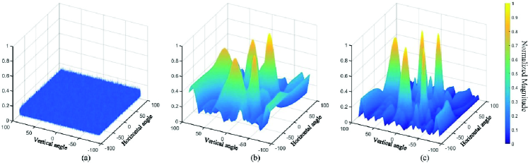
Figure 4: Comparison of beam patterns, where $N_{\rm BS}^{\rm RF}=N_{\rm UD}^{\rm RF}=4$ and the AoAs of the 5 MPCs are known to the UD: (a) Random transmit precoding matrix with $8\times 8$ UPA, (b) Multi-beam transmit precoding matrix with $8\times 8$ UPA, and (c) Multi-beam transmit precoding matrix with $16\times 16$ UPA.

From $\bar{\bm{A}}_{\rm BS}\!=\!\bm{J}_{u}\widetilde{\bm{W}}_{u}^{\rm H}\bm{A}_{\rm BS}^{*}$, we observe that $\widetilde{\bm{W}}_{u}$ may destroy the shift-invariance structure of $\bm{A}_{\rm BS}$. Similar to downlink CE, we can design $\widetilde{\bm{W}}_{u}$ using Algorithm 1 by replacing the input parameters $N_{d}$, $N_{\rm s}^{d}$, $N_{\rm UD}^{\rm RF}$, $N_{\rm UD}^{\rm h}$, $N_{\rm UD}^{\rm v}$, $M_{\rm UD}^{\rm h}$ and $M_{\rm UD}^{\rm v}$ for UD with $N_{u}$, $N_{\rm s}^{u}$, $N_{\rm BS}^{\rm RF}$, $N_{\rm BS}^{\rm h}$, $N_{\rm BS}^{\rm v}$, $M_{\rm BS}^{\rm h}$ and $M_{\rm BS}^{\rm v}$ for BS. By substituting the designed $\widetilde{\bm{W}}_{u}$ into (22), we obtain

$$\bar{\bm{Y}}_{u}=\bm{A}_{\bm{\tau}{\rm BS}}\bar{\bm{S}}_{u}+\check{\bm{N}}_{u}^{\rm T},$$ (23)

where $\bar{\bm{S}}_{u}\!=\!\text{diag}(\bm{\alpha})\left(\bm{A}_{\rm UD}^{\rm T}\bm{F}_{u}\bm{S}_{u}\right)$, and $\bm{A}_{\bm{\tau}{\rm BS}}\!\in\!\mathbb{C}^{KM_{\rm BS}^{\rm v}M_{\rm BS}^{\rm h}\times L}$ is given by

$$\begin{split}\bm{A}_{\bm{\tau}{\rm BS}}&=\bm{A}_{\bm{\tau}}\odot\big{(}\bm{J}_{u}\widetilde{\bm{W}}_{u}^{\rm H}\left(\left(\bm{A}_{\rm BS}^{\nu}\right)^{*}\odot\left(\bm{A}_{\rm BS}^{\mu}\right)^{*}\right)\big{)}\\ &=\bm{A}_{\bm{\tau}}\odot\bar{\bm{A}}_{\rm BS}^{\nu}\odot\bar{\bm{A}}_{\rm BS}^{\mu}.\end{split}$$ (24)

In (24), $\bar{\bm{A}}_{\rm BS}^{\mu}\!\in\!\mathbb{C}^{M_{\rm BS}^{\rm h}\times L}$ ($\bar{\bm{A}}_{\rm BS}^{\nu}\!\in\!\mathbb{C}^{M_{\rm BS}^{\rm v}\times L}$) is the sub-matrix consisting of the first $M_{\rm BS}^{\rm h}$ ($M_{\rm BS}^{\rm v}$) rows of $\left(\bm{A}_{\rm BS}^{\mu}\right)^{*}$ ($\left(\bm{A}_{\rm BS}^{\nu}\right)^{*}$). In this way, $\widetilde{\bm{W}}_{u}$ visualizes the high-dimensional hybrid analog/digital array as a low-dimensional digital array, and $\bm{A}_{\bm{\tau}{\rm BS}}$ holds the triple shift-invariance structure for horizontal/vertical AoDs and delays [35]. Therefore, we can apply the MDU-ESPRIT algorithm to obtain the super-resolution estimates of horizontal/vertical AoDs and delays, $\big{\{}\widehat{\theta}_{l}^{\rm BS},\widehat{\varphi}_{l}^{\rm BS},\widehat{\tau}_{l}\big{\}}_{l=1}^{\widehat{L}}$.

III-B Design Multi-Beam Transmit Precoding Matrix at UD

We design the transmit precoding matrix $\bm{F}_{u}\!=\!\bm{F}_{{\rm RF},u}\bm{F}_{{\rm BB},u}$ at UD by exploiting the estimate $\big{\{}\widehat{\theta}_{l}^{\rm UD},\widehat{\varphi}_{l}^{\rm UD}\big{\}}_{l=1}^{\widehat{L}}$ obtained at the downlink CE stage so that the UD with the limited transmit power can transmit directional multi-beam signals for improving the received SNR at the BS.

We first consider the analog transmit precoding matrix $\bm{F}_{{\rm RF},u}\!\in\!\mathbb{C}^{N_{\rm UD}\times N_{\rm UD}^{\rm RF}}$. The estimate $\widehat{\bm{A}}_{\rm UD}$ of the array response matrix $\bm{A}_{\rm UD}$ can be calculated given the estimated AoAs $\big{\{}\widehat{\theta}_{l}^{\rm UD},\widehat{\varphi}_{l}^{\rm UD}\big{\}}_{l=1}^{\widehat{L}}$. To fully exploit the acquired $\big{\{}\widehat{\theta}_{l}^{\rm UD},\widehat{\varphi}_{l}^{\rm UD}\big{\}}_{l=1}^{\widehat{L}}$, the multi-beam transmit precoding matrix should align its $\widehat{L}$ beams with the $\widehat{L}$ estimated AoAs. Specifically, the phase shifters of the PSN at UD can be divided into the $\widehat{L}$ groups as equally as possible, depending on $\widehat{L}$ and $N_{\rm UD}^{\rm RF}$.

Case I: $\widehat{L}>N_{\rm UD}^{\rm RF}$. This is the case that the number of beams transmitted by UD is larger than that of RF chains. For the UD equipped with the hybrid array with the fully-connected PSN, there are $N_{\rm PS}\!=\!N_{{\rm UD}}^{{\rm RF}}N_{{\rm UD}}$ phase shifters. Let the number of phase shifters assigned to the $l$th group be $n_{{\rm ps},l}$ with $1\leq l\leq\widehat{L}$. We introduce the $\widehat{L}$-dimensional vector $\bm{v}_{\rm ps}$ as

$$\vspace{-1.0mm}\bm{v}_{\rm ps}=\big{[}n_{{\rm ps},1}\cdots n_{{\rm ps},\widehat{L}}\big{]}^{\rm T}=n_{\rm ps}\bm{1}_{\widehat{L}}+\big{[}\bm{1}_{n_{\rm re}}^{\rm T}~{}\bm{0}_{\widehat{L}-n_{\rm re}}^{\rm T}\big{]}^{\rm T},\vspace{-1.0mm}$$ (25)

where $n_{\rm ps}\!=\!\lfloor N_{\rm PS}/\widehat{L}\rfloor$ and $n_{\rm re}\!=\!\text{mod}\big{(}N_{\rm PS},\widehat{L}\big{)}$. By defining the index vector $\bm{p}\!=\!\left[1~{}2\cdots N_{\rm PS}\right]^{\rm T}$, the ordered index set ${\cal P}_{l}$ of the $l$th group can be obtained as ${\cal P}_{l}\!=\!\bm{p}_{\left[\sum\nolimits_{i=1}^{l-1}n_{{\rm ps},i}+1:\sum\nolimits_{i=1}^{l}n_{{\rm ps},i}\right]}$ with $|{\cal P}_{l}|_{c}\!=\!n_{{\rm ps},l}$. Then, we can define the vector $\bm{f}\!=\!\big{[}\bm{f}_{1}^{\rm T}\cdots\bm{f}_{\widehat{L}}^{\rm T}\big{]}^{\rm T}\!\in\!\mathbb{C}^{N_{\rm PS}}$, where $\!\bm{f}_{l}\!=\!\widehat{\bm{A}}_{{\rm UD}\left[\text{mod}\left({\cal P}_{l},N_{\rm UD}\right),l\right]}^{*}\!\in\!\mathbb{C}^{n_{{\rm ps},l}}$ for $1\!\leq\!l\!\leq\!\widehat{L}$, to obtain $\bm{F}_{{\rm RF},u}\!=\!\text{mat}\left(\bm{f};N_{\rm UD},N_{\rm UD}^{\rm RF}\right)$.

Case II: $\widehat{L}\leq N_{\rm UD}^{\rm RF}$ and $N_{\rm UD}^{\rm RF}$ can be divided exactly by $\widehat{L}$. The $N_{\rm UD}^{\rm RF}$ RF chains can be equally allocated to the $\widehat{L}$ groups, and we can choose $\bm{F}_{{\rm RF},u}\!=\!\bm{1}_{N_{\rm rep}}^{\rm T}\otimes\widehat{\bm{A}}_{\rm UD}^{*}$, with $N_{\rm rep}\!=\!N_{\rm UD}^{\rm RF}/\widehat{L}$.

Case III: $\widehat{L}<N_{\rm UD}^{\rm RF}$ and $N_{\rm UD}^{\rm RF}$ cannot be divided exactly by $\widehat{L}$. In this case, we have $\bm{F}_{{\rm RF},u}\!=\!\left[\bm{F}_{{\rm RF},u}^{1}~{}\bm{F}_{{\rm RF},u}^{2}\right]$, where $\bm{F}_{{\rm RF},u}^{1}\!\in\!\mathbb{C}^{N_{\rm UD}\times\widehat{L}N_{\rm rep}}$ with $N_{\rm rep}\!=\!\lfloor N_{\rm UD}^{\rm RF}/\widehat{L}\rfloor$ and $\bm{F}_{{\rm RF},u}^{2}\!\in\!\mathbb{C}^{N_{\rm UD}\times N_{{\rm UD},{\rm re}}^{\rm RF}}$ with $N_{{\rm UD},{\rm re}}^{\rm RF}\!=\!\text{mod}\big{(}N_{\rm UD}^{\rm RF},\widehat{L}\big{)}$. We can design $\bm{F}_{{\rm RF},u}^{1}\!=\!\bm{1}_{N_{\rm rep}}^{\rm T}\!\otimes\!\widehat{\bm{A}}_{\rm UD}^{*}$ similar to Case II, and we can choose $\bm{F}_{{\rm RF},u}^{2}\!=\!\text{mat}\big{(}\big{[}\widetilde{\bm{f}}_{1}^{\rm T}\cdots\widetilde{\bm{f}}_{\widehat{L}}^{\rm T}\big{]}^{\rm T};N_{\rm UD},N_{{\rm UD},{\rm re}}^{\rm RF}\big{)}$ similar to Case I, where $\widetilde{\bm{f}}_{l}$ can be acquired by using $N_{{\rm UD},{\rm re}}^{\rm RF}$ instead of $N_{\rm UD}^{\rm RF}$ in Case I.

Due to the limited resolution of the PSN, the phase value of every element in the designed $\bm{F}_{{\rm RF},u}$ is quantized to the nearest value in the phase set ${\cal A}$. As for the digital transmit precoding matrix $\bm{F}_{{\rm BB},u}\!\in\!\mathbb{C}^{N_{\rm UD}^{\rm RF}\times N_{\rm s}^{u}}$, we can design its element as $\left[\bm{F}_{{\rm BB},u}\right]_{j_{1},j_{2}}\!=\!e^{\textsf{j}2\pi b_{j_{1},j_{2}}}$ with $b_{j_{1},j_{2}}\sim{\cal U}[0,~{}1]$. Finally, we obtain the multi-beam transmit precoding matrix $\bm{F}_{u}\!=\!\bm{F}_{{\rm RF},u}\bm{F}_{{\rm BB},u}$.

To intuitively compare $\bm{F}_{d}$ of the BS designed at the downlink CE stage and $\bm{F}_{u}$ of the UD designed at the uplink CE stage, we provide the comparison of beam patterns in Fig. 4, where we have $N_{{\rm BS}}^{{\rm RF}}\!=\!N_{{\rm UD}}^{{\rm RF}}\!=\!4$ RF chains at the BS and each UD, and the AoAs of the $5$ MPCs are known to the UD. Specifically, Fig. 4 (a) depicts the beam pattern of the random transmit precoding matrix $\bm{F}_{d}$ for the $8\!\times\!8$ UPA, while Fig. 4 (b) and Fig. 4 (c) plot the beam patterns of the multi-beam transmit precoding matrices $\bm{F}_{u}$ for the $8\!\times\!8$ and $16\!\times\!16$ UPAs, respectively. Compared with the beam pattern of Fig. 4 (a), the beam pattern in Fig. 4 (b) has 5 mainlobes aligned with the directions of the AoAs of the 5 MPCs, which can significantly improve the SNR at receiver. Moreover, by comparing Fig. 4 (b) with Fig. 4 (c), it can be observed that the sidelobes of the multi-beam signals are further suppressed when the array size increases. In a nutshell, the proposed multi-beam transmit precoding matrix design enables the UD with limited transmit power to form the directional signals with multiple beams aligned with the estimated AoAs of the MPCs for improving the uplink CE performance.

IV MDU-ESPRIT Algorithm

Because the aggregated receive combining matrix $\widetilde{\bm{W}}_{d}$ ($\widetilde{\bm{W}}_{u}$) designed at the UD (BS) reconstructs the double (triple) shift-invariance structure of array response, spectrum estimation techniques can be utilized to estimate the channel parameters. We consider $R$-dimensional ($R$-D) unitary ESPRIT algorithm with $R\!\geq\!2$. Without loss of generality, we define a general signal transmission model for the channel consisting of $L$ MPCs and $R$ sets of spatial frequencies as

$$\bm{Y}=\bm{A}\bm{S}+\bm{N},$$ (26)

where $\bm{Y}\!\in\!\mathbb{C}^{M\times N}$ is the received data matrix aggregated over $N$ snapshots, $M\!=\!\prod\nolimits_{r=1}^{R}M_{r}$, with $M_{r}$ being the dimension of the parameter vector associated with the $r$th spatial frequency for $1\!\leq\!r\!\leq\!R$, and $\bm{S}\!\in\!\mathbb{C}^{L\times N}$ and $\bm{N}\!\in\!\mathbb{C}^{M\times N}$ are the transmit signal and noise matrices, respectively, while the array response matrix $\bm{A}\!\in\!\mathbb{C}^{M\times L}$ is given by

$$\begin{split}\bm{A}&=\bm{A}_{\mu_{R}}\odot\cdots\odot\bm{A}_{\mu_{2}}\odot\bm{A}_{\mu_{1}}\\ &=\left[\bm{a}\left(\mu_{1}^{1},\mu_{1}^{2},\cdots,\mu_{1}^{R}\right)\cdots\bm{a}\left(\mu_{L}^{1},\mu_{L}^{2},\cdots,\mu_{L}^{R}\right)\right].\end{split}$$ (27)

In (27), $\bm{A}_{\mu_{r}}\!=\!\left[\bm{a}(\mu_{1}^{r})\cdots\bm{a}(\mu_{L}^{r})\right]\!\in\!\mathbb{C}^{M_{r}\times L}$ is the steering matrix related to the $r$th set of spatial frequencies $\{\mu_{l}^{r}\}_{l=1}^{L}$, with $\bm{a}\left(\mu_{l}^{r}\right)\!=\!\left[1~{}e^{\textsf{j}\mu_{l}^{r}}\cdots e^{\textsf{j}(M_{r}-1)\mu_{l}^{r}}\right]^{\rm T}\!\in\!\mathbb{C}^{M_{r}}$ being the $l$th steering vector, while the array response vector $\bm{a}\left(\mu_{l}^{1},\mu_{l}^{2},\cdots,\mu_{l}^{R}\right)\!\in\!\mathbb{C}^{M}$ related to the $l$th MPC is given by

$$\bm{a}\left(\mu_{l}^{1},\mu_{l}^{2},\cdots,\mu_{l}^{R}\right)=\bm{a}\left(\mu_{l}^{R}\right)\otimes\cdots\otimes\bm{a}\left(\mu_{l}^{2}\right)\otimes\bm{a}\left(\mu_{l}^{1}\right).$$ (28)

The MDU-ESPRIT algorithm, which acquires the super-resolution estimates of the $R$ sets of spatial frequencies from (26), denoted by $\left\{\widehat{\mu}_{l}^{r}\right\}_{l=1}^{L}$ for $1\!\leq\!r\!\leq\!R$, consists of the five steps.

IV-1 $R$-D Spatial Smoothing Preprocessing (SSP)

In order to take into account the insufficient measurement dimension $N$ caused by the limited training overhead, we will exploit the spatial smoothing technique [31] to preprocess the original data matrix $\bm{Y}$ of (26). This preprocessing can mitigate the influence of other coherent signals and avoid the rank deficiency of the covariance matrix of $\bm{S}$ to enhance robustness. Specifically, we first define the $R$ spatial smoothing parameters $\{G_{r}\}_{r=1}^{R}$ with $1\!\leq\!G_{r}\!\leq\!M_{r}$, and obtain the sub-dimensions $\{M_{r}^{\rm sub}\}_{r=1}^{R}$ corresponding to $\{M_{r}\}_{r=1}^{R}$ as $M_{r}^{\rm sub}\!=\!M_{r}\!-\!G_{r}\!+\!1$ for $1\!\leq\!r\!\leq\!R$. Thus the size of total sub-dimension is $M_{\rm sub}\!=\!\prod\nolimits_{r=1}^{R}M_{r}^{\rm sub}$. To obtain the $R$-D selection matrix, we next define the $g_{r}$th ‘1-D’ selection matrix as $\bm{J}^{(g_{r})}\!=\!\left[\bm{O}_{M_{r}^{\rm sub}\times(g_{r}-1)}~{}\bm{I}_{M_{r}^{\rm sub}}~{}\bm{O}_{M_{r}^{\rm sub}\times(G_{r}-g_{r})}\right]\!\in\!\mathbb{R}^{M_{r}^{\rm sub}\times M_{r}}$ for $1\!\leq\!g_{r}\!\leq\!G_{r}$. Then, we can obtain $G\!=\!\prod\nolimits_{r=1}^{R}G_{r}$ ‘$R$-D’ selection matrices, with the $(g_{1},g_{2},\cdots,g_{R})$th ‘$R$-D’ selection matrix given by $\bm{J}_{g_{1},g_{2},\cdots,g_{R}}\!=\!\bm{J}^{(g_{R})}\otimes\cdots\otimes\bm{J}^{(g_{2})}\otimes\bm{J}^{(g_{1})}\!\in\!\mathbb{R}^{M_{\rm sub}\times M}$. By applying these $R$-D selection matrices to $\bm{Y}$, the smoothed complex-valued data matrix $\bar{\bm{Y}}\!\in\!\mathbb{C}^{M_{\rm sub}\times NG}$ is obtained as

$$\begin{split}\bar{\bm{Y}}=&\big{[}\left(\bm{J}_{1,1,\cdots\!,1,1}\bm{Y}\right)\,\cdots\,\left(\bm{J}_{1,1,\cdots\!,1,G_{R}}\bm{Y}\right)\,\left(\bm{J}_{1,1,\cdots\!,2,1}\bm{Y}\right)\\ &\left(\bm{J}_{1,1,\cdots\!,2,2}\bm{Y}\right)\,\cdots\,\left(\bm{J}_{G_{1},G_{2},\cdots\!,G_{R-1},G_{R}}\bm{Y}\right)\big{]}.\end{split}$$ (29)

IV-2 Real-Valued Processing (RVP)

To reduce the computational complexity, the forward backward averaging technique [30] is utilized to transform $\bar{\bm{Y}}$ into the real-valued matrix $\bar{\bm{Y}}_{\rm re}\!\in\!\mathbb{R}^{M_{\rm sub}\times 2NG}$

$$\bar{\bm{Y}}_{\rm re}=\bm{Q}_{M_{\rm sub}}^{\rm H}\left[\bar{\bm{Y}}~{}\left(\bm{\varPi}_{M_{\rm sub}}\bar{\bm{Y}}^{*}\bm{\varPi}_{NG}\right)\right]\bm{Q}_{2NG},$$ (30)

where $\bm{\varPi}_{n}$ is the exchange matrix of size $n\times n$ that permutates the row order of $\bm{I}_{n}$, and $\bm{Q}_{n}\!\in\!\mathbb{C}^{n\times n}$ is a sparse unitary matrix satisfying $\bm{\varPi}_{n}\bm{Q}_{n}^{\rm H}\!=\!\bm{Q}_{n}$.

IV-3 Signal Subspace Approximation (SSA)

To extract the information of spatial frequencies from the real-valued matrix $\bar{\bm{Y}}_{\rm re}$, we introduce the transform steering matrix $\bm{K}$ which satisfies [30]

$$\Re\left\{\bm{Q}_{m_{r}}^{\rm H}\bm{J}_{r}\bm{Q}_{M_{\rm sub}}\right\}\bm{K}\bm{\varLambda}_{r}=\Im\left\{\bm{Q}_{m_{r}}^{\rm H}\bm{J}_{r}\bm{Q}_{M_{\rm sub}}\right\}\bm{K},$$ (31)

where $1\leq r\leq R$, $m_{r}\!=\!M_{\rm sub}\left(M_{r}^{\rm sub}\!-\!1\right)/M_{r}^{\rm sub}$, and $\bm{\varLambda}_{r}\!=\!\text{diag}\big{(}\left[\tan\left(\mu_{1}^{r}/2\right)\cdots\tan\left(\mu_{L}^{r}/2\right)\right]^{\rm T}\big{)}$ is the real-valued diagonal matrix involving the desired spatial frequencies $\{\mu_{l}^{r}\}_{l=1}^{L}$, while $\bm{J}_{r}\!=\!\bm{I}_{\prod\nolimits_{i=r+1}^{R}M_{i}^{\rm sub}}\!\otimes\!\widetilde{\bm{J}}^{(r)}\!\otimes\!\bm{I}_{\prod\nolimits_{i=1}^{r-1}M_{i}^{\rm sub}}\!\in\!\mathbb{R}^{m_{r}\times M_{\rm sub}}$, with $\widetilde{\bm{J}}^{(r)}\!=\!\left[\bm{0}_{M_{r}^{\rm sub}-1}~{}\bm{I}_{M_{r}^{\rm sub}-1}\right]$. Note that $\bm{K}$ is related to the approximate signal subspace matrix $\bm{E}_{\rm s}\!\in\!\mathbb{R}^{M_{\rm sub}\times L}$ corresponding to the underlying signal subspace. Specifically, since the columns of $\bm{K}$ and $\bm{E}_{\rm s}$ span the same $L$-dimensional signal subspace [31, 35], $\bm{K}\!=\!\bm{E}_{\rm s}\bm{T}$, where $\bm{T}\!\in\!\mathbb{R}^{L\times L}$ is a non-singular matrix. To determine $\bm{E}_{\rm s}$, we take the left singular vectors corresponding to the largest $L$ singular values of $\bar{\bm{Y}}_{\rm re}$ as $\bm{E}_{\rm s}$. Specifically, from the real-valued partial singular values decomposition (SVD) of $\bar{\bm{Y}}_{\rm re}\!=\!\bm{U}_{\rm re}\bm{\varSigma}_{\rm re}\bm{V}_{\rm re}^{\rm H}$, we have $\bm{E}_{\rm s}\!=\!\bm{U}_{{\rm re}[:,1:L]}$.

IV-4 Shift-Invariance Equation Solving (SIES)

Based on the acquired approximate signal subspace $\bm{E}_{\rm s}$, we use $\bm{K}\!=\!\bm{E}_{\rm s}\bm{T}$ in (31) to obtain the $R$ shift-invariance equations

$$\Re\left\{\bm{Q}_{m_{r}}^{\rm H}\bm{J}_{r}\bm{Q}_{M_{\rm sub}}\right\}\bm{E}_{\rm s}\bm{\varPhi}_{r}=\Im\left\{\bm{Q}_{m_{r}}^{\rm H}\bm{J}_{r}\bm{Q}_{M_{\rm sub}}\right\}\bm{E}_{\rm s},$$ (32)

where $\bm{\varPhi}_{r}\!=\!\bm{T}\bm{\varLambda}_{r}\bm{T}^{-1}\!\in\!\mathbb{R}^{L\times L}$ for $1\leq r\leq R$. To estimate the diagonal matrices $\{\bm{\varLambda}_{r}\}_{r=1}^{R}$, we first obtain the estimates of the $R$ real-valued matrices $\{\bm{\varPhi}_{r}\}_{r=1}^{R}$, denoted as $\big{\{}\widehat{\bm{\varPhi}}_{r}\big{\}}_{r=1}^{R}$, by applying the LS or total least squares (TLS) estimator to solve the $R$ shift-invariance equations of (32).

IV-5 $R$-D Joint Diagonalization (JD)

From the estimated $\widehat{\bm{\varPhi}}_{r}\!=\!\bm{T}\widehat{\bm{\varLambda}}_{r}\bm{T}^{-1}$ with $\widehat{\bm{\varLambda}}_{r}$ denoting the estimate of $\bm{\varLambda}_{r}$ for $1\!\leq\!r\!\leq\!R$, we exploit the following $R$-D joint diagonalization to obtain the paired estimates of the spatial frequencies $\left\{\widehat{\mu}_{l}^{r}\right\}_{l=1}^{L}$ from $\big{\{}\widehat{\bm{\varLambda}}_{r}\big{\}}_{r=1}^{R}$. Specifically, we consider the two cases of $R\!=\!2$ and $R\!\geq\!3$. For $R\!=\!2$, namely, the 2-D case, since $\widehat{\bm{\varPhi}}_{1}$ and $\widehat{\bm{\varPhi}}_{2}$ share the same eigenvector matrix $\bm{T}$, we can calculate the EVD of the complex-valued matrix $\bm{\varPsi}\!=\!\widehat{\bm{\varPhi}}_{1}\!+\!\textsf{j}\widehat{\bm{\varPhi}}_{2}$ to obtain $\widehat{\bm{\varLambda}}_{1}$ and $\widehat{\bm{\varLambda}}_{2}$, specifically, $\bm{\varPsi}\!=\!\bm{T}\bm{\varDelta}\bm{T}^{-1}$ with $\bm{\varDelta}\!=\!\widehat{\bm{\varLambda}}_{1}\!+\!\textsf{j}\widehat{\bm{\varLambda}}_{2}$, and $\widehat{\bm{\varLambda}}_{1}\!=\!\Re\{\bm{\varDelta}\}$ and $\widehat{\bm{\varLambda}}_{2}\!=\!\Im\{\bm{\varDelta}\}$. For $R\!\geq\!3$, the noise-corrupted matrices $\big{\{}\widehat{\bm{\varPhi}}_{r}\big{\}}_{r=1}^{R}$ do not always exactly share the same $\bm{T}$. Hence, we exploit the simultaneous Schur decomposition (SSD) algorithm [37], which is developed from the real Schur decomposition [40] for multi-parameter estimation and pairing. By utilizing the SSD algorithm, we obtain the $R$ approximate upper-triangular matrices $\left\{\bm{\varGamma}_{r}\right\}_{r=1}^{R}$ so that $\big{\{}\widehat{\bm{\varLambda}}_{r}\big{\}}_{r=1}^{R}$ are acquired as the main diagonal elements of $\left\{\bm{\varGamma}_{r}\right\}_{r=1}^{R}$, i.e., $\widehat{\bm{\varLambda}}_{r}\!=\!\text{diag}\left(\text{vdiag}(\bm{\varGamma}_{r})\right)$, for $1\!\leq\!r\!\leq\!R$. Finally, the $R$ paired super-resolution estimates of the spatial frequencies $\left\{\widehat{\mu}_{l}^{r}\right\}_{l=1}^{L}$ can be calculated from $\widehat{\bm{\varLambda}}_{r}$ as $\widehat{\mu}_{l}^{r}\!=\!2\arctan\big{(}\big{[}\widehat{\bm{\varLambda}}_{r}\big{]}_{l,l}\big{)}$ for $1\!\leq\!l\!\leq\!L$ and $1\!\leq\!r\!\leq\!R$.

This MDU-ESPRIT algorithm is summarized in Algorithm 2. At the downlink CE stage, we estimate $\left\{\widehat{\mu}_{l}^{\rm UD},\widehat{\nu}_{l}^{\rm UD}\right\}_{l=1}^{\widehat{L}}$ based on $\bar{\bm{Y}}_{d}$ of (11) by applying the 2-D ($R\!=\!2$) unitary ESPRIT algorithm. Furthermore, based on $\bar{\bm{Y}}_{u}$ of (23), $\left\{\widehat{\mu}_{l}^{\rm BS},\widehat{\nu}_{l}^{\rm BS},\widehat{\mu}_{l}^{\tau}\right\}_{l=1}^{\widehat{L}}$ are estimated using the 3-D ($R\!=\!3$) unitary ESPRIT algorithm at the uplink CE stage. Hence, the spatial smoothing parameters for Algorithm 2 in the 2-D and 3-D cases are $\{G_{1}^{d},G_{2}^{d}\}$ and $\{G_{1}^{u},G_{2}^{u},G_{3}^{u}\}$, respectively. The corresponding total sub-dimension sizes at the UD and BS are $M_{\rm sub}^{\rm UD}\!=\!(M_{\rm UD}^{\rm h}\!-\!G_{1}^{d}\!+\!1)(M_{\rm UD}^{\rm v}\!-\!G_{2}^{d}\!+\!1)$ and $M_{\rm sub}^{\rm BS}\!=\!(M_{\rm BS}^{\rm h}\!-\!G_{1}^{u}\!+\!1)(M_{\rm BS}^{\rm v}\!-\!G_{2}^{u}\!+\!1)(K\!-\!G_{3}^{u}\!+\!1)$, respectively.

Algorithm 2 MDU-ESPRIT Algorithm

0:  Data matrix $\bm{Y}$, number of MPCs $L$, sub-dimensions $\{M_{r}\}_{r=1}^{R}$, spatial smoothing parameters $\{G_{r}\}_{r=1}^{R}$

0:  Super-resolution estimates of spatial frequencies $\left\{\widehat{\mu}_{l}^{r}\right\}_{l=1}^{L}$, $1\leq r\leq R$

1:  Obtain smoothed data matrix $\bar{\bm{Y}}$ (29) using $R$-D spatial smoothing preprocessing

2:  Obtain real-valued data matrix $\bar{\bm{Y}}_{\rm re}$ (30) using forward backward averaging

3:  Determine approximate signal subspace matrix $\bm{E}_{\rm s}$ through SVD

4:  Solve shift-invariance equations (32) to obtain $R$ real-valued matrices $\big{\{}\widehat{\bm{\varPhi}}_{r}\big{\}}_{r=1}^{R}$

5:  Perform $R$-D joint diagonalization to estimate diagonal matrices $\big{\{}\widehat{\bm{\varLambda}}_{r}\big{\}}_{r=1}^{R}$: i) $R=2$, calculate EVD of $\bm{\varPsi}=\widehat{\bm{\varPhi}}_{1}+\textsf{j}\widehat{\bm{\varPhi}}_{2}=\bm{T}\bm{\varDelta}\bm{T}^{-1}$ to obtain $\widehat{\bm{\varLambda}}_{1}=\Re\{\bm{\varDelta}\}$ and $\widehat{\bm{\varLambda}}_{2}=\Im\{\bm{\varDelta}\}$; ii) $R\geq 3$, obtain $R$ diagonal matrices $\big{\{}\widehat{\bm{\varLambda}}_{r}\big{\}}_{r=1}^{R}$ via SSD algorithm

6:  Extract $R$ paired $\left\{\widehat{\mu}_{l}^{r}\right\}_{l=1}^{L}$ from $\big{\{}\widehat{\bm{\varLambda}}_{r}\big{\}}_{r=1}^{R}$

V ML Pairing and Path Gains Estimation

At the downlink CE stage, the BS obtains the estimated horizontal/vertical AoAs $\left\{\bar{\theta}_{l}^{\rm UD},\bar{\varphi}_{l}^{\rm UD}\right\}_{l=1}^{\widehat{L}}$ fed back by the UD. It then estimates the horizontal/vertical AoDs and delays $\big{\{}\widehat{\theta}_{l}^{\rm BS},\!\widehat{\varphi}_{l}^{\rm BS},\!\widehat{\tau}_{l}\big{\}}_{l=1}^{\widehat{L}}$ at the uplink CE stage. Since $\left\{\bar{\theta}_{l}^{\rm UD},\!\bar{\varphi}_{l}^{\rm UD}\right\}_{l=1}^{\widehat{L}}$ and $\big{\{}\widehat{\theta}_{l}^{\rm BS},\!\widehat{\varphi}_{l}^{\rm BS},\!\widehat{\tau}_{l}\big{\}}_{l=1}^{\widehat{L}}$ are acquired in the two different ends of the channel at two different stages, it is necessary to pair them. Furthermore, the path gain vector $\bm{\alpha}$ needs to be estimated. We propose to apply an ML approach to pair the channel parameters and to estimate the path gains, which corresponds to Step 7 of Fig. 2 at the BS.

Specifically, according to (24), we construct the equivalent steering matrix associated with $\big{\{}\widehat{\theta}_{l}^{\rm BS},\widehat{\varphi}_{l}^{\rm BS},\widehat{\tau}_{l}\big{\}}_{l=1}^{\widehat{L}}$ as $\widehat{\bm{A}}_{\tau{\rm BS}}$, where $\{\widehat{\tau}_{l}\}_{l=1}^{\widehat{L}}$ are arranged in ascending order. Based on the estimated horizontal/vertical AoAs fed back to the BS, $\left\{\bar{\theta}_{l}^{\rm UD},\bar{\varphi}_{l}^{\rm UD}\right\}_{l=1}^{\widehat{L}}$, we can reconstruct the estimated multi-beam transmit precoding matrix, denoted by $\widehat{\bm{F}}_{u}$, similar to the construction of $\bm{F}_{u}$ given in Section III-B. Clearly, there are a total of $J_{\rm c}\!=\!\widehat{L}!$ possible ordered combinations or pairs $\big{\{}\bar{\theta}_{l_{j}}^{\rm UD},\bar{\varphi}_{l_{j}}^{\rm UD}\big{\}}_{l_{j}=1}^{\widehat{L}}$ that can pair with $\widehat{\bm{A}}_{\tau{\rm BS}}$ or $\big{\{}\widehat{\theta}_{l}^{\rm BS},\widehat{\varphi}_{l}^{\rm BS},\widehat{\tau}_{l}\big{\}}_{l=1}^{\widehat{L}}$, where $j\!\in\!{\cal J}$ and the size of the ordered set ${\cal J}$ is $|{\cal J}|_{c}\!=\!J_{\rm c}$. For each $\big{\{}\bar{\theta}_{l_{j}}^{\rm UD},\bar{\varphi}_{l_{j}}^{\rm UD}\big{\}}_{l_{j}=1}^{\widehat{L}}$, we can establish the corresponding array response matrix $\bm{A}_{\rm UD}$, which is denoted as $\widehat{\bm{A}}_{{\rm UD},j}$. Thus, for each pair of the AoDs and AoAs, we have $\widehat{\bm{A}}_{\tau{\rm BS}}$, $\widehat{\bm{A}}_{{\rm UD},j}$ and $\widehat{\bm{F}}_{u}$. Substituting them into (20) yields $\check{\bm{y}}_{u}\!=\!\widehat{\bm{A}}_{j}\bm{\alpha}_{j}\!+\check{\bm{n}}_{u}$, where $\widehat{\bm{A}}_{j}\!=\!\widehat{\bm{A}}_{\tau{\rm BS}}\!\odot\!\big{(}\widehat{\bm{A}}_{{\rm UD},j}^{\rm T}\widehat{\bm{F}}_{u}\bm{S}_{u}\big{)}^{\rm T}$ while $\bm{\alpha}_{j}$ is the path gain vector corresponding to the $j$th pair of the AoDs and AoAs with $j\!\in\!{\cal J}$. The LS estimate of $\bm{\alpha}_{j}$ is readily given as

$$\widehat{\bm{\alpha}}_{j}=\big{(}\widehat{\bm{A}}_{j}^{\rm H}\widehat{\bm{A}}_{j}\big{)}^{-1}\widehat{\bm{A}}_{j}^{\rm H}\check{\bm{y}}_{u}.$$ (33)

From the estimate $\widehat{\bm{\alpha}}_{j}$, we can estimate $\check{\bm{y}}_{u}$ according to $\widehat{\check{\bm{y}}}_{u,j}\!=\!\widehat{\bm{A}}_{j}\widehat{\bm{\alpha}}_{j}$ with the residual $\big{\|}\check{\bm{y}}_{u}\!-\!\widehat{\check{\bm{y}}}_{u,j}\big{\|}_{2}^{2}$. We can then find the optimal pair index $j^{\star}$ by solving the following optimization problem

$$j^{\star}=\arg\min\limits_{j\in{\cal J}}\big{\|}\check{\bm{y}}_{u}-\widehat{\check{\bm{y}}}_{u,j}\big{\|}_{2}^{2}.$$ (34)

Hence, the optimal estimate of the path gains is given by $\widehat{\bm{\alpha}}\!=\!\widehat{\bm{\alpha}}_{j^{\star}}\!=\!\beta\left[\widehat{\alpha}_{1}\cdots\widehat{\alpha}_{\widehat{L}}\right]^{\rm T}$ and we have the optimal ordered mmWave channel parameter estimate $\big{\{}\bar{\theta}_{l}^{\rm UD},\bar{\varphi}_{l}^{\rm UD},\widehat{\theta}_{l}^{\rm BS},\widehat{\varphi}_{l}^{\rm BS},\widehat{\tau}_{l},\widehat{\alpha}_{l}\big{\}}_{l=1}^{\widehat{L}}$.

By substituting $\big{\{}\bar{\theta}_{l}^{\rm UD},\bar{\varphi}_{l}^{\rm UD},\widehat{\theta}_{l}^{\rm BS},\widehat{\varphi}_{l}^{\rm BS},\widehat{\tau}_{l},\widehat{\alpha}_{l}\big{\}}_{l=1}^{\widehat{L}}$ into (7), we obtain the optimally estimated frequency-domain channel matrix $\widehat{\bm{H}}[k]$ at the $k$th subcarrier as

$$\widehat{\bm{H}}[k]\!=\!\beta\sum\limits_{l=1}^{\widehat{L}}\widehat{\alpha}_{l}\bm{a}_{\rm UD}\left(\bar{\mu}_{l}^{\rm UD},\bar{\nu}_{l}^{\rm UD}\right)\bm{a}_{\rm BS}^{\rm H}\left(\widehat{\mu}_{l}^{\rm BS},\widehat{\nu}_{l}^{\rm BS}\right)e^{-\textsf{j}2\pi\frac{kf_{s}}{K}\widehat{\tau}_{l}},$$ (35)

where $\bar{\mu}_{l}^{\rm UD}\!=\!\pi\sin(\bar{\theta}_{l}^{\rm UD})\cos(\bar{\varphi}_{l}^{\rm UD})$ and $\bar{\nu}_{l}^{\rm UD}\!=\!\pi\sin(\bar{\varphi}_{l}^{\rm UD})$, while $\widehat{\mu}_{l}^{\rm BS}\!=\!\pi\sin\big{(}\widehat{\theta}_{l}^{\rm BS}\big{)}\cos\left(\widehat{\varphi}_{l}^{\rm BS}\right)$ and $\widehat{\nu}_{l}^{\rm BS}\!=\!\pi\sin\left(\widehat{\varphi}_{l}^{\rm BS}\right)$.

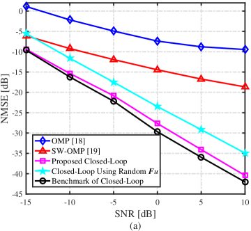
(a)

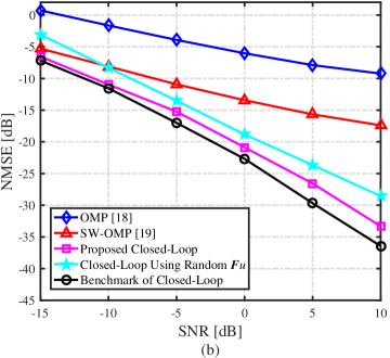
(b)

Figure 5: NMSE performance comparison of different CE schemes versus SNRs with the same training overhead $T_{\rm CE}=132$: (a) the number of MPCs $L=3$; and (b) $L=5$.

VI Performance Evaluation

An extensive simulation investigation is carried out to evaluate the CE performance and computational complexity of the proposed closed-loop CE scheme. In simulations, the carrier frequency is $f_{c}\!=\!30$ GHz with the bandwidth $f_{s}\!=\!200$ MHz, the numbers of RF chains at BS and UD are both 4, i.e., $N_{\rm BS}^{\rm RF}\!=\!N_{\rm UD}^{\rm RF}\!=\!4$, and the numbers of horizontal and vertical antennas at BS and UD are both 12, i.e., $N_{\rm BS}^{\rm h}\!=\!N_{\rm BS}^{\rm v}\!=\!N_{\rm UD}^{\rm h}\!=\!N_{\rm UD}^{\rm v}\!=\!12$, and the quantization accuracy of the PSN is defined by $N_{q}^{\rm ps}\!=\!3$ bits, while the feedback quantization accuracy for AoAs is specified by $N_{q}^{\rm ang}\!=\!10$ bits. Without loss of generality, the case of single UD $Q\!=\!1$ is considered. From Fig. 3, it is clear that for the generic case of $Q>1$, the uplink training overhead becomes $N_{u}N_{\rm o}^{u}$ instead of $QN_{u}N_{\rm o}^{u}$ for the case of $Q=1$. The channel model is simulated as follows. Each of the path gains $\{\alpha_{l}\}_{l=1}^{L}$ is generated according to ${\cal CN}(0,1)$, while the other channel parameters $\{\tau_{l},\theta_{l}^{\rm UD},\theta_{l}^{\rm BS},\varphi_{l}^{\rm UD},\varphi_{l}^{\rm BS}\}_{l=1}^{L}$ all follow uniform distribution, specifically, $\tau_{l}\!\sim\!{\cal U}[0,~{}\tau_{\max}]$ and $\theta_{l}^{\rm UD},\theta_{l}^{\rm BS},\varphi_{l}^{\rm UD},\varphi_{l}^{\rm BS}\!\sim\!{\cal U}\left[-\pi/3~{}\pi/3\right]$ for the $l$th MPC. The maximum multipath delay is set to $\tau_{\max}\!=\!16T_{s}$, i.e., $N_{\rm c}\!=\!16$. The number of subcarriers is set to $K\!=\!128$ with the length of cyclic prefix (CP) being 32, and perfect frame synchronization is assumed. In our proposed solution, the sizes of low-dimensional digital sub-arrays visualized from the high-dimensional hybrid arrays are set to $M_{\rm BS}^{\rm h}\!=\!M_{\rm BS}^{\rm v}\!=\!M_{\rm UD}^{\rm h}\!=\!M_{\rm UD}^{\rm v}\!=\!8$. Hence, the numbers of downlink and uplink training time slots are $N_{d}\!=\!22$ and $N_{u}\!=\!22$, respectively, given the number of downlink independent signal streams $N_{\rm s}^{d}\!=\!N_{\rm UD}^{\rm RF}\!-\!1\!=\!3$ and the number of uplink independent signal streams $N_{\rm s}^{u}\!=\!N_{\rm BS}^{\rm RF}\!-\!1\!=\!3$. Additionally, $P\!=\!8$ adjacent subcarriers are jointly employed to estimate the number of MPCs, with the threshold parameter $\varepsilon$ empirically set to 1.54, 0.50, 0.16, 0.05, 0.016, and 0.005, respectively, at the SNR of -15 dB, -10 dB, -5 dB, 0 dB, 5 dB, and 10 dB. The spatial smoothing parameters used for Algorithm 2 are $G_{1}^{d}\!=\!G_{2}^{d}\!=\!G_{1}^{u}\!=\!G_{2}^{u}\!=\!2$ and $G_{3}^{u}\!=\!K/2$. The downlink and uplink SNRs are both defined as $\rho\sigma_{\alpha}^{2}/\sigma_{n}^{2}$, where $\rho$ and $\sigma_{n}^{2}$ are the transmit power and receiver noise variance, respectively.

The state-of-the-art OMP-based frequency-domain scheme [18] and the SW-OMP-based scheme [19] are adopted as two benchmarks. In order to be consistent with [18] and [19], their digital transmit precoding/receive combining matrices are taken as the identity matrix, while the design of analog counterparts is similar to the construction of $\bm{F}_{{\rm RF},d}[m]$ given in Section II-B. The sizes of the quantized angle-domain grids associated with horizontal/vertical AoAs/AoDs, denoted by $G_{\rm BS}^{\rm h}$, $G_{\rm BS}^{\rm v}$, $G_{\rm UD}^{\rm h}$ and $G_{\rm UD}^{\rm v}$, are set to twice the numbers of antennas in the horizontal and vertical directions of UPA, respectively, according to [18, 19], i.e., $G_{\rm BS}\!=\!G_{\rm BS}^{\rm h}\times G_{\rm BS}^{\rm v}\!=\!2N_{\rm BS}^{\rm h}\times 2N_{\rm BS}^{\rm v}\!=\!24\times 24$ and $G_{\rm UD}\!=\!G_{\rm UD}^{\rm h}\times G_{\rm UD}^{\rm v}\!=\!2N_{\rm UD}^{\rm h}\times 2N_{\rm UD}^{\rm v}\!=\!24\times 24$. Furthermore, all CE schemes adopt the same training overhead, which is equal to the required number of training frames [18, 19], to ensure the fairness of comparison.

VI-A CE Performance Evaluation

First the CE performance is evaluated using the normalized mean square error (NMSE) metric given by

$$\text{NMSE}=\mathbb{E}\bigg{(}\sum\limits_{k=0}^{K-1}\big{\|}\bm{H}[k]-\widehat{\bm{H}}[k]\big{\|}_{F}^{2}\Big{/}\sum\limits_{k=0}^{K-1}\big{\|}\bm{H}[k]\big{\|}_{F}^{2}\bigg{)}.$$ (36)

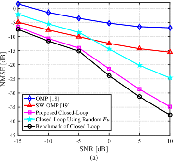
(a)

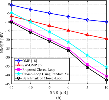
(b)

Figure 6: NMSE performance comparison of different CE schemes versus SNRs with the same number of MPCs $L=4$: (a) training overhead $T_{\rm CE}=88$; and (b) $T_{\rm CE}=176$.

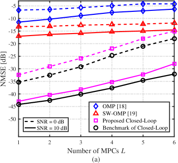
(a)

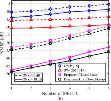
(b)

Figure 7: NMSE performance comparison of different CE schemes versus the number of MPCs $L$ with $\text{SNR}=0$ dB and 10 dB: (a) training overhead $T_{\rm CE}=88$; and (b) $T_{\rm CE}=176$.

Fig. 5 compares the NMSE performance of the proposed closed-loop scheme with those of the OMP and SW-OMP based schemes for different SNRs, given the numbers of MPCs $L=3$ and $L=5$. For our closed-loop scheme, the numbers of OFDM symbols in each downlink time slot and uplink time slot are $N_{\rm o}^{d}\!=\!N_{\rm o}^{u}\!=\!3$. Therefore, the training overhead of our closed-loop scheme is $T_{\rm CE}\!=\!N_{d}N_{\rm o}^{d}\!+\!N_{u}N_{\rm o}^{u}\!=\!132$. In Fig. 5, the NMSE curve labeled as ‘Proposed Close-Loop’ is our proposed closed-loop CE scheme, which also estimates the number of MPCs $L$, while the curve labeled with ‘Benchmark of Closed-Loop’ is the closed-loop scheme given the perfect knowledge of $L$, which provides a lower bound NMSE. It can be seen that the CE accuracy achieved by our closed-loop scheme with no knowledge of $L$ is very close to this lower bound, which demonstrates the super-resolution accuracy of our solution Additionally, our closed-loop CE scheme adopting the random transmit precoding matrix $\bm{F}_{u}$ is also illustrated in Fig. 5, where it is observed to suffer from around 5 dB and 3 dB performance losses in the cases of $L=3$ and 5, respectively. This clearly demonstrates the effectiveness of the proposed multi-beam transmit precoding matrix design which fully exploits the estimated horizontal/vertical AoAs to optimize the received SNR for improving CE performance. Furthermore, the results of Fig. 5 show that our proposed closed-loop CE scheme dramatically outperforms the two CS-based schemes, in terms of CE accuracy. In particular, the OMP and SW-OMP based schemes seem to suffer from the NMSE floor at high SNR. By adopting larger discrete angle-domain grids to achieve larger quantized CS dictionary, the performance of these CS-based schemes can be improved [18, 19] at the expense of significantly increased computational complexity, which becomes unaffordable for FD-MIMO systems with massive antenna array.

Fig. 6 compares the NMSE performance of different CE schemes against different SNRs, given two training overheads with the same number of MPCs $L=4$. $T_{\rm CE}\!=\!88$ in Fig. 6a and $T_{\rm CE}\!=\!176$ in Fig. 6b correspond to choosing $N_{\rm o}^{d}\!=\!N_{\rm o}^{u}\!=\!2$ and $N_{\rm o}^{d}\!=\!N_{\rm o}^{u}\!=\!4$ in our scheme, respectively. From Fig. 6, similar conclusions to those observed for Fig. 5 can be obtained. In particular, it can be seen that our closed-loop CE scheme considerably outperforms the two CS-based schemes.

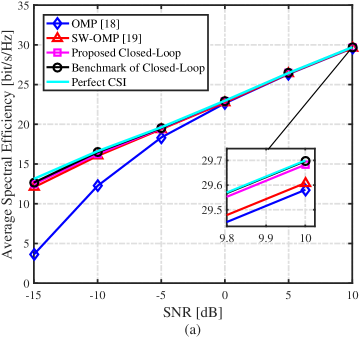
(a)

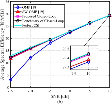
(b)

Figure 8: ASE performance comparison of different CE schemes versus SNRs: (a) the number of MPCs $L=3$; and (b) $L=5$.

Fig. 7 compares the NMSE performance of different CE schemes versus the number of MPCs $L$ given two SNR values of 0 dB and 10 dB as well as two training overheads of $T_{\rm CE}=88$ and $T_{\rm CE}=176$. In simulations, we adopted the same parameter settings as in Fig. 6 except the number of MPCs. From Fig. 7, the good performance of the proposed multi-beam transmit precoding matrix design and EVD-based approach for MPCs’ number estimation is evident. Again, the proposed closed-loop scheme significantly outperforms two other CS-based schemes. Observe that the performance gain of our scheme over the two other schemes increases for sparser mmWave channels, i.e., having smaller number of MPCs. Moreover, although the performance gap between the proposed solution and the CS-based methods is gradually reduced at low SNRs as the number of MPCs $L$ increases, the proposed scheme can achieve the considerable performance gain over the CS schemes at high SNRs. Hence, the proposed scheme is suitable for sparse mmWave channels, and more performance gain can be obtained for sparser channels.

TABLE I: Computational Complexity of Proposed Closed-Loop Scheme

Operation	Complexity
Step 1(b)&5(b)	$\textsf{O}\left(N_{d}N_{\rm UD}N_{\rm UD}^{\rm RF}(1+N_{\rm s}^{d})+N_{u}N_{\rm BS}N_{\rm BS}^{\rm RF}(1+N_{\rm s}^{u})\right)$
Step 2	$\textsf{O}\big{(}\left(N_{\rm UD}^{\rm sub}\right)^{3}\!+\!\left(N_{\rm UD}^{\rm sub}\right)^{2}N_{\rm o}^{d}N_{P}\big{)}$
Step 3 ($R=2$)	$\textsf{O}\bigg{(}\underbrace{M_{\rm sub}^{\rm UD}KN_{\rm o}^{d}G_{1}^{d}G_{2}^{d}}_{\rm 2-D\,SSP}\!\!+\!\!\underbrace{8M_{\rm sub}^{\rm UD}KN_{\rm o}^{d}G_{1}^{d}G_{2}^{d}}_{\rm RVP}\!\!+\!\!\underbrace{\textstyle\frac{1}{4}M_{\rm sub}^{\rm UD}\widehat{L}^{2}}_{\rm SSA}\!\!+\!\!\underbrace{\textstyle\frac{1}{2}\left(\widehat{L}^{3}\!\!+\!\!2\widehat{L}^{2}M_{\rm sub}^{\rm UD}\!\!+\!\!2(\widehat{L}\!\!+\!\!1)(M_{\rm sub}^{\rm UD})^{2}\right)}_{\rm SIES}\!\!+\!\!\underbrace{\textstyle\frac{1}{4}\widehat{L}^{3}}_{\rm 2-D\,JD}\bigg{)}$
Step 6 ($R=3$)	$\textsf{O}\bigg{(}\underbrace{M_{\rm sub}^{\rm BS}N_{\rm o}^{u}G_{1}^{u}G_{2}^{u}G_{3}^{u}}_{\rm 3-D\,SSP}\!\!+\!\!\underbrace{8M_{\rm sub}^{\rm BS}N_{\rm o}^{u}G_{1}^{u}G_{2}^{u}G_{3}^{u}}_{\rm RVP}\!\!+\!\!\underbrace{\textstyle\frac{1}{4}M_{\rm sub}^{\rm BS}\widehat{L}^{2}}_{\rm SSA}\!\!+\!\!\underbrace{\textstyle\frac{3}{4}\left(\widehat{L}^{3}\!\!+\!\!2\widehat{L}^{2}M_{\rm sub}^{\rm BS}\!\!+\!\!2(\widehat{L}\!\!+\!\!1)(M_{\rm sub}^{\rm BS})^{2}\right)}_{\rm SIES}\!\!+\!\!\underbrace{\textstyle\frac{3}{4}\widehat{L}^{4}}_{\rm 3-D\,JD}\bigg{)}$
Step 7	$\textsf{O}\big{(}\widehat{L}!(\widehat{L}^{3}\!+\!2\widehat{L}^{2}KN_{\rm BS}^{\rm sub}N_{\rm o}^{u})\big{)}$
Step 8	$\textsf{O}\big{(}K\widehat{L}N_{\rm BS}N_{\rm UD}\big{)}$

Next we consider the average spectral efficiency (ASE) performance metric [41] defined as

$$\begin{split}\text{A}&\text{SE}=\frac{1}{K}\sum\nolimits_{k=0}^{K-1}\log_{2}\det\big{(}\bm{I}_{N_{\rm s}}\\ &+{\textstyle{1\over{N_{\rm s}}}}\bm{R}_{n}^{-1}[k]\bm{W}_{c}^{\rm H}[k]\bm{H}[k]\bm{F}_{p}[k]\bm{F}_{p}^{\rm H}[k]\bm{H}^{\rm H}[k]\bm{W}_{c}[k]\big{)},\end{split}$$ (37)

where $\bm{R}_{n}[k]\!=\!\sigma_{n}^{2}\bm{W}_{c}^{\rm H}[k]\bm{W}_{c}[k]$, $\bm{F}_{p}[k]\!=\!\bm{F}_{{\rm RF},p}\bm{F}_{{\rm BB},p}[k]$ and $\bm{W}_{c}[k]\!=\!\bm{W}_{{\rm RF},c}\bm{W}_{{\rm BB},c}[k]$ are the transmit precoding and receive combining matrices used during data transmission, respectively, while $N_{\rm s}$ is the number of transmit data stream. The principle component analysis (PCA)-based hybrid beamforming scheme proposed in [41] is used to evaluate the ASE performance, where the CSI is based on the estimated channels. Besides, the spectral efficiency of the PCA-based hybrid beamforming scheme with the perfect CSI known both to the BS and UD is adopted as the performance upper bound. Here, the same simulation parameters used in Fig. 5 are considered, and the number of transmit data streams used is $N_{\rm s}\!=\!2$ in (37). Fig. 8 compares the ASE performance of different CE schemes against different SNRs. It can be observed from Fig. 8 that the ASE performance using the CSI estimated by the proposed scheme closely matches to the performance upper bound obtained using the perfect CSI at both the BS and UD. It can also be seen that the ASE performance gain achieved by the proposed scheme over the two CS-based schemes is 0.1 [bit/s/Hz] at high SNR conditions. At low SNRs, this gain is clearly larger. Note that the ASE performance of the OMP based scheme is particularly poor when $\text{SNR}\!\leq\!0$ dB.

VI-B Computational Complexity Evaluation

The computational complexity analysis of our closed-loop CE scheme is detailed in Table I, where the notation $\textsf{O}(N)$ stands for ‘on order of $N$’. The computational requirements of Step 1(a) and Step 5(a) are omitted, since they are much smaller, compared with the requirements of other steps. Clearly, Step 4 does not involve computation. It can be seen that the computational requirements are dominated by Step 6 (corresponding to Algorithm 2 with $R\!=\!3$) and Step 7. Also observe that the complexity of the CE scheme increases fast as $\widehat{L}$ increases, since the computational complexity of Step 6 and Step 7 are proportional to $\widehat{L}^{4}$ and $\widehat{L}!$, respectively.

TABLE II: Computational Complexity of Two CS-Based CE Schemes

Operation	OMP-based Scheme [18]	SW-OMP-based Scheme [19]
Measurement matrix	$\textsf{O}\left(KT_{\rm CE}N_{\rm BS}^{\rm RF}N_{\rm BS}N_{\rm UD}G_{\rm BS}G_{\rm UD}\right)$	$\textsf{O}\left(T_{\rm CE}N_{\rm BS}^{\rm RF}N_{\rm BS}N_{\rm UD}G_{\rm BS}G_{\rm UD}\right)$
Whitening	NA	$\textsf{O}\left(T_{\rm CE}N_{\rm BS}^{\rm RF}\left((T_{\rm CE}N_{\rm BS}^{\rm RF})^{2}+K+G_{\rm BS}G_{\rm UD}\right)\right)$
Correlation	$\textsf{O}\big{(}T_{\rm CE}N_{\rm BS}^{\rm RF}G_{\rm BS}G_{\rm UD}\big{(}\sum\nolimits_{k=1}^{K}I_{k}\big{)}\big{)}$	$\textsf{O}\left(T_{\rm CE}N_{\rm BS}^{\rm RF}G_{\rm BS}G_{\rm UD}KI\right)$
Project subspace	$\textsf{O}\big{(}\sum\nolimits_{k=1}^{K}\big{(}\frac{1}{4}I_{k}^{2}\left(I_{k}+1\right)^{2}+\frac{1}{3}I_{k}\left(I_{k}+1\right)\left(2I_{k}+1\right)T_{\rm CE}N_{\rm BS}^{\rm RF}\big{)}\big{)}$	$\textsf{O}\big{(}\frac{1}{4}I^{2}(I+1)^{2}+\frac{1}{3}KI(I+1)(2I+1)T_{\rm CE}N_{\rm BS}^{\rm RF}\big{)}$
Update residual	$\textsf{O}\big{(}T_{\rm CE}N_{\rm BS}^{\rm RF}\big{(}\sum\nolimits_{k=1}^{K}\frac{I_{k}}{2}\left(I_{k}+1\right)\big{)}\big{)}$	$\textsf{O}\big{(}T_{\rm CE}N_{\rm BS}^{\rm RF}K\frac{I}{2}(I+1)\big{)}$
Compute MSE	$\textsf{O}\big{(}T_{\rm CE}N_{\rm BS}^{\rm RF}\big{(}\sum\nolimits_{k=}^{K}I_{k}\big{)}\big{)}$	$\textsf{O}\left(T_{\rm CE}N_{\rm BS}^{\rm RF}K^{2}I\right)$
Reestablishment	$\textsf{O}\big{(}N_{\rm BS}N_{\rm UD}\big{(}\sum\nolimits_{k=1}^{K}I_{k}\big{)}\big{)}$	$\textsf{O}\left(N_{\rm BS}N_{\rm UD}KI\right)$

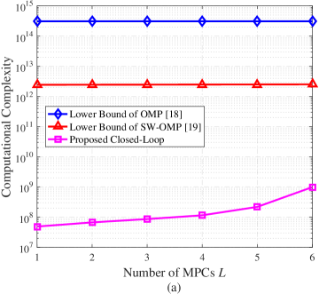
(a)

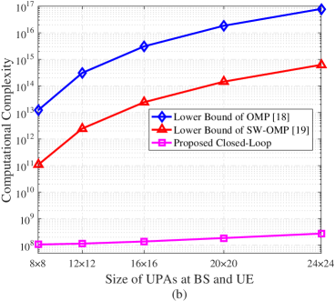
(b)

Figure 9: Computational complexity comparison of different CE schemes given the training overhead $T_{\rm CE}=88$: (a) sizes of UPAs at BS and UD are both $12\times 12$; and (b) number of MPCs $L=4$.

The computational complexity of the two CS-based CE schemes is given in Table II for comparison, where the numbers of iterations for the OMP algorithm at the $k$th subcarrier and the SW-OMP algorithm are denoted by $I_{k}$ and $I$, respectively. Note that the values of $I_{k}$ are different for different subcarriers. It can be seen that the computational complexity of these two CS-based schemes increase fast as the quantized grids $G_{\rm BS}$ and $G_{\rm UD}$ increase. Also the complexity of the OMP scheme is around $K$ times of the SW-OMP scheme, because the $K$ subchannels at $K$ subcarriers are independently estimated in the OMP scheme but they are jointly estimated in the SW-OMP scheme. Due to the power leakage caused by the mismatch between the discrete CS angle-domain dictionary and continuously distributed AoAs/AoDs of channels, the number of effective MPCs represented in the redundant CS dictionary are usually greater than $L$. Hence, the value of $I_{k}$ in the OMP scheme and the value of $I$ in the SW-OMP scheme are not fixed and they are usually greater than $L$. Therefore, we can use $I\!=\!I_{k}\!=\!L$ to provide the lower bounds of the computational complexity for the two CS-based schemes.

Fig. 9 compares the computational complexity of our closed-loop CE scheme with those of the two CS-based schemes given the training overhead $T_{\rm CE}=88$ corresponding to $N_{\rm o}^{d}\!=\!N_{\rm o}^{u}\!=\!2$ in our scheme. From Fig. 9a, we observe that the computational complexity of the proposed CE solution increases slightly as the number of MPCs increase. Most strikingly, however, given the size of UPA as $12\times 12$, the complexity of our solution is at least 3 orders of magnitude lower than the SW-OMP scheme and at least 5 orders of magnitude lower than the OMP scheme. The results of Fig. 9b indicate that given $L\!=\!4$, the complexity of our solution is almost immune to the size of UPA at the BS and UD. By contrast, the complexity of the two CS-based schemes increase considerably as the number of antennas increases. Again, the complexity of our solution is several orders of magnitude lower than the other two schemes. It should also be reiterated that to mitigate the power leakage, the CS-based schemes adopt the high-dimensional redundant dictionary, which results in unaffordable storage space requirements when the number of antennas is large. Clearly, for FD-MIMO systems with massive number of antennas, the proposed closed-loop scheme offers considerable advantage over the CS-based schemes, in terms of both computational complexity and storage requirements.

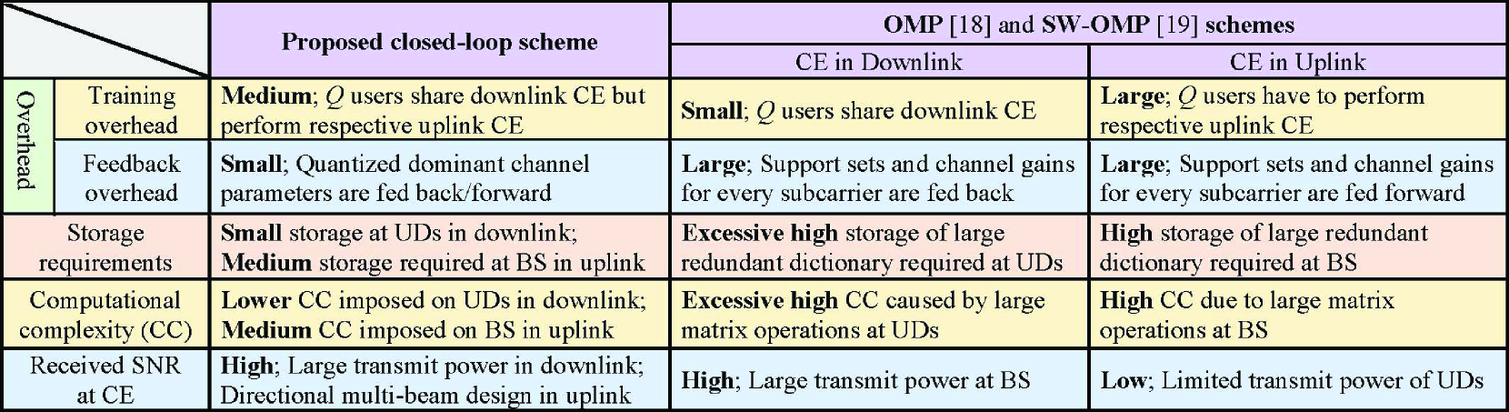
TABLE III. Comparison of Advantages and Disadvantages of Different CE Schemes

The advantages and disadvantages of our proposed solution and two other CS-based CE schemes are given in Table III, where the training/feedback overhead, storage requirements, computational complexity and received SNR at CE are compared.

VII Conclusions

We have proposed a closed-loop sparse CE scheme for multi-user wideband mmWave FD-MIMO systems with hybrid beamforming. By exploiting the sparsity of mmWave channels in both angle and delay domains and by visualizing high-dimensional hybrid arrays as low-dimensional digital arrays, the proposed scheme is capable of obtaining the super-resolution estimates of horizontal/vertical AoDs/AoAs and delays based on the MDU-ESPRIT algorithm. Specifically, at the downlink CE stage, we design the common random transmit precoding matrix at the BS and the receive combining matrix at each UD to estimate the horizontal/vertical AoAs of sparse MPCs. At the uplink CE stage, based on the designed receive combining matrix at the BS, we estimate horizontal/vertical AoDs and delays. Furthermore, the AoAs estimated at each UD are utilized to design the multi-beam transmit precoding matrix for further enhancing CE performance. We also propose an ML approach at the BS to pair the channel parameters acquired at the two stages and to optimally estimate the path gains. Simulation results have demonstrated that the proposed closed-loop CE scheme offers considerable advantages over state-of-the-art CS-based CE schemes, in terms of providing significantly more accurate CSI estimate while imposing dramatically lower computational complexity and storage requirements.

Sampling the delay-domain continuous $\bm{H}_{q}(\tau)$ in (3) with the sampling period $T_{s}$ yields

$$\begin{split}\bm{H}_{q}(nT_{s})&=\beta_{q}\sum\limits_{l=1}^{L_{q}}\bm{H}_{q,l}p\left(\tau\!-\!\tau_{q,l}\right)\circledast\sum\limits_{n=-\infty}^{\infty}\delta\left(\tau\!-\!nT_{s}\right)\\[-4.2679pt] &=\beta_{q}\sum\limits_{n=-\infty}^{\infty}\sum\limits_{l=1}^{L_{q}}\bm{H}_{q,l}p\left(nT_{s}-\tau_{q,l}\right),\end{split}$$ (38)

where $\circledast$ and $\delta(\cdot)$ represent the linear convolution operation and Dirac delta function, respectively. The Fourier transform of $\bm{H}_{q}(nT_{s})$ is then given by

$$\bm{H}_{q}(f)\!=\!\frac{\beta_{q}}{T_{s}}\sum\limits_{l=1}^{L_{q}}\sum\limits_{n=-\infty}^{\infty}\bm{H}_{q,l}P(f)e^{-\textsf{j}2\pi f\tau_{q,l}}\delta\left(f\!-\!nf_{s}\right),$$ (39)

where $P(f)$ is the Fourier transform of $p(\tau)$. Obviously, $\bm{H}_{q}(f)$ exhibits periodicity with period $f_{s}$. Thus, $\bm{H}_{q}(f)$ within a period of $f\in\left[-f_{s}/2,~{}f_{s}/2\right]$ can be expressed as

$$\bm{H}_{q}(f)\!=\!\frac{\beta_{q}}{T_{s}}\sum\limits_{l=1}^{L_{q}}P(f)\bm{H}_{q,l}e^{-\textsf{j}2\pi f\tau_{q,l}}\!\approx\!\frac{\beta_{q}}{T_{s}}\sum\limits_{l=1}^{L_{q}}C\bm{H}_{q,l}e^{-\textsf{j}2\pi f\tau_{q,l}}.$$ (40)

The approximation in (40) is valid because the PSF $p(\tau)$ is designed to realize the ideal passband filter characteristics of $P(f)=C$ for $f\in\left[-f_{s}/2,~{}f_{s}/2\right]$ and $P(f)\approx 0$ for $f\notin\left[-f_{s}/2,~{}f_{s}/2\right]$. For convenience, we consider $C=T_{s}$. Therefore, the frequency-domain channel matrix $\bm{H}_{q}[k]$ at the $k$th subcarrier, where $0\leq k\leq K-1$, can be written as

$$\bm{H}_{q}[k]=\bm{H}_{q}\bigg{(}\frac{kf_{s}}{K}\bigg{)}=\beta_{q}\sum\limits_{l=1}^{L_{q}}\bm{H}_{q,l}e^{-\textsf{j}\frac{2\pi kf_{s}\tau_{q,l}}{K}}.$$ (41)

References

- [1] Z. Xiao, T. He, P. Xia, and X.-G. Xia, “Hierarchical codebook design for beamforming training in millimeter-wave communication,” IEEE Trans. Wireless Commun., vol. 15, no. 5, pp. 3380-3392, May 2016.
- [2] Z. Gao, L. Dai, D. Mi, Z. Wang, M. A. Imran, and M. Z. Shakir, “Mmwave massive-MIMO-based wireless backhaul for the 5G ultra-dense network,” IEEE Wireless Commun., vol. 22, no. 5, pp. 13-21, Oct. 2015.
- [3] W. Ma and C. Qi, “Beamspace channel estimation for millimeter wave massive MIMO system with hybrid precoding and combining,” IEEE Trans. Signal Process., vol. 66, no. 18, pp. 4839-4853, Sep. 2018.
- [4] Y. Huang, J. Zhang, and M. Xiao, “Constant envelope hybrid precoding for directional millimeter-wave communications,” IEEE J. Sel. Areas Commun., vol. 36, no. 4, pp. 845-859, Apr. 2018.
- [5] A. Liu and V. K. N. Lau, “Impact of CSI knowledge on the codebook-based hybrid beamforming in massive MIMO,” IEEE Trans. Signal Process., vol. 64, no. 24, pp. 6545-6556, Dec. 2016.
- [6] A. Liu, V. K. N. Lau, and M.-J. Zhao, “Stochastic successive convex optimization for two-timescale hybrid precoding in massive MIMO,” IEEE J. Sel. Topics Signal Process., vol. 12, no. 3, pp. 432-444, Jun. 2018.
- [7] J. Zhang, Y. Huang, Q. Shi, J. Wang, and L. Yang, “Codebook design for beam alignment in millimeter wave communication systems,” IEEE Trans. Commun., vol. 65, no. 11, pp. 4980-4995, Nov. 2017.
- [8] Wireless LAN Medium Access Control (MAC) and Physical Layer (PHY) Specifications. Amendment 3: Enhancements for Very High Throughput in the 60 GHz Band, IEEE Std. 802.11ad, 2012.
- [9] M. Kokshoorn, H. Chen, P. Wang, Y. Li, and B. Vucetic, “Millimeter wave MIMO channel estimation using overlapped beam patterns and rate adaptation,” IEEE Trans. Signal Process., vol. 65, no. 3, pp. 601-616, Feb. 2017.
- [10] Z. Xiao, P. Xia, and X.-G. Xia, “Codebook design for millimeter-wave channel estimation with hybrid precoding structure,” IEEE Trans. Wireless Commun., vol. 16, no. 1, pp. 141-153, Jan. 2017.
- [11] Z. Xiao, P. Xia, and X.-G. Xia, “Channel estimation and hybrid precoding for millimeter-wave MIMO systems: A low-complexity overall solution,” IEEE Access, vol. 5, pp. 16100-16110, Aug. 2017.
- [12] J. Lee, G. T. Gil, and Y. H. Lee, “Channel estimation via orthogonal matching pursuit for hybrid MIMO systems in millimeter wave communications,” IEEE Trans. Commun., vol. 64, no. 6, pp. 2370-2386, Jun. 2016.
- [13] Y. Wu, Y. Gu, and Z. Wang, “Channel estimation for mmWave MIMO with transmitter hardware impairments,” IEEE Commun. Lett., vol. 22, no. 2, pp. 320-323, Feb. 2018.
- [14] Z. Zhou, J. Fang, L. Yang, H. Li, Z. Chen, and S. Li, “Channel estimation for millimeter-wave multiuser MIMO systems via PARAFAC decomposition,” IEEE Trans. Wireless Commun., vol. 15, no. 11, pp. 7501-7516, Nov. 2016.
- [15] R. W. Heath, Jr., N. González-Prelcic, S. Rangan, W. Roh, and A. M. Sayeed, “An overview of signal processing techniques for millimeter wave MIMO systems,” IEEE J. Sel. Topics Signal Process., vol. 10, no. 3, pp. 436-453, Apr. 2016.
- [16] Z. Gao, C. Hu, L. Dai, and Z. Wang, “Channel estimation for millimeter-wave massive MIMO with hybrid precoding over frequency-selective fading channels,” IEEE Commun. Lett., vol. 20, no. 6, pp. 1259-1262, Jun. 2016.
- [17] Y. Dong, C. Chen, N. Yi, G. Lu, and Y. Jin, “Channel estimation using low-resolution PSs for wideband mmWave systems,” in Proc. VTC2017-Spring (Sydney, Australia), Jun. 4-7, 2017, pp. 1-5.
- [18] K. Venugopal, A. Alkhateeb, N. González-Prelcic, and R. W. Heath, “Channel estimation for hybrid architecture-based wideband millimeter wave systems,” IEEE J. Sel. Areas Commun., vol. 35, no. 9, pp. 1996-2009, Sep. 2017.
- [19] J. Rodríguez-Fernández, N. González-Prelcic, K. Venugopal, and R. W. Heath, “Frequency-domain compressive channel estimation for frequency-selective hybrid millimeter wave MIMO systems,” IEEE Trans. Wireless Commun., vol. 17, no. 5, pp. 2946-2960, May 2018.
- [20] X. Ma et al., “Design and optimization on training sequence for mmWave communications: A new approach for sparse channel estimation in massive MIMO,” IEEE J. Sel. Areas Commun., vol. 35, no. 7, pp. 1486-1497, Jul. 2017.
- [21] Z. Zhou, J. Fang, L. Yang, H. Li, Z. Chen, and R. S. Blum, “Low-rank tensor decomposition-aided channel estimation for millimeter wave MIMO-OFDM systems,” IEEE J. Sel. Areas Commun., vol. 35, no. 7, pp. 1524-1538, Jul. 2017.
- [22] B. Wang, F. Gao, S. Jin, H. Lin, and G. Y. Li, “Spatial- and frequency-wideband effects in millimeter-wave massive MIMO systems,” IEEE Trans. Signal Process., vol. 66, no. 13, pp. 3393-3406, Jul. 2018.
- [23] Y. Tsai, L. Zheng, and X. Wang, “Millimeter-wave beamformed full-dimensional MIMO channel estimation based on atomic norm minimization,” IEEE Trans. Commun., vol. 66, no. 12, pp. 6150-6163, Dec. 2018.
- [24] C. Hu, L. Dai, T. Mir, Z. Gao, and J. Fang, “Super-resolution channel estimation for mmWave massive MIMO with hybrid precoding,” IEEE Trans. Veh. Technol., vol. 67, no. 9, pp. 8954-8958, Sep. 2018.
- [25] Z. Xiao, P. Xia, and X.-G. Xia, “Enabling UAV cellular with millimeter-wave communication: Potentials and approaches,” IEEE Commun. Mag., vol. 54, no. 5, pp. 66-73, May 2016.
- [26] C. Zhang, W. Zhang, W. Wang, L. Yang, and W. Zhang, “Research challenges and opportunities of UAV millimeter-wave communications,” IEEE Wireless Commun., vol. 26, no. 1, pp. 58-62, Feb. 2019.
- [27] P. Yu et al.,“Capacity enhancement for 5G networks using mmWave aerial base stations: Self-organizing architecture and approach,” IEEE Wireless Commun., vol. 25, no. 4, pp. 58-64, Aug. 2018.
- [28] S. Jaeckel, L. Raschkowski, K. Börner, L. Thiele, F. Burkhardt, and E. Eberlein, “Quasi deterministic radio channel generator: User manual and documentation,” Fraunhofer Heinrich Hertz Institute, Tech. Rep. v2.2.0, 2019.
- [29] S. Jaeckel, L. Raschkowski, K. Börner, and L. Thiele, “QuaDRiGa: A 3-D multicell channel model with time evolution for enabling virtual field trials,” IEEE Trans. Antennas Propag., vol. 62, no. 6, pp. 3242-3256, Jun. 2014.
- [30] M. D. Zoltowski, M. Haardt, and C. P. Mathews, “Closed-form 2-D angle estimation with rectangular arrays in element space or beamspace via unitary ESPRIT,” IEEE Trans. Signal Process., vol. 44, no. 2, pp. 316-328, Feb. 1996.
- [31] A.-J. van der Veen, M. C. Vanderveen, and A. Paulraj, “Joint angle and delay estimation using shift-invariance techniques,” IEEE Trans. Signal Process., vol. 46, no. 2, pp. 405-418, Feb. 1998.
- [32] L. Zhao, D. W. K. Ng, and J. Yuan, “Multi-user precoding and channel estimation for hybrid millimeter wave systems,” IEEE J. Sel. Areas Commun., vol. 35, no. 7, pp. 1576-1590, Jul. 2017.
- [33] Z. Gao, L. Dai, S. Han, C.-L. I, Z. Wang, and L. Hanzo, “Compressive sensing techniques for next-generation wireless communications,” IEEE Wireless Commun., vol. 25, no. 4, pp. 144-153, Jun. 2018.
- [34] J. Ma, S. Zhang, H. Li, F. Gao, and S. Jin, “Sparse bayesian learning for the time-varying massive MIMO channels: Acquisition and tracking,” IEEE Trans. Commun., vol. 67, no. 3, pp. 1925 C1938, Mar. 2019.
- [35] M. C. Vanderveen, A.-J. Van der Veen, and A. Paulraj, “Estimation of multipath parameters in wireless communications,” IEEE Trans. Signal Process., vol. 46, no. 3, pp. 682-690, Mar. 1998.
- [36] J. Mao, Z. Gao, Y. Wu, and M. Alouini, “Over-sampling codebook-based hybrid minimum sum-mean-square-error precoding for millimeter-wave 3D-MIMO,” IEEE Wireless Commun. Lett., vol. 7, no. 6, pp. 938-941, Dec. 2018.
- [37] M. Haardt and J. A. Nossek, “Simultaneous Schur decomposition of several nonsymmetric matrices to achieve automatic pairing in multidimensional harmonic retrieval problems,” IEEE Trans. Signal Process., vol. 46, no. 1, pp. 161-169, Jan. 1998.
- [38] D. L. Donoho, “De-noising by soft-thresholding,” IEEE Trans. Inf. Theory, vol. 41, no. 3, pp. 613-627, May 1995.
- [39] Z. Xiao, X. Xia, and L. Bai, “Achieving antenna and multipath diversities in GLRT-based burst packet detection,” IEEE Trans. Signal Process., vol. 63, no. 7, pp. 1832-1845, Apr. 2015.
- [40] G. H. Golub and C. F. Van Loan, Matrix Computations (4th ed.). Baltimore, MD, USA: The Johns Hopkins Univ. Press, 2013.
- [41] Y. Sun, Z. Gao, H. Wang, and D. Wu, “Wideband hybrid precoding for next-generation backhaul/fronthaul based on mmWave FD-MIMO,” in Proc. IEEE Globecom Workshops (Abu Dhabi, UAE), Dec. 9-13, 2018, pp. 1-6.
- [42] Z. Xiao, C. Zhang, D. Jin, and N. Ge, “GLRT approach for robust burst packet acquisition in wireless communications,” IEEE Trans. Wireless Commun., vol. 12, no. 3, pp. 1127-1137, Mar. 2013.