Adaptive isogeometric boundary element methods
with local smoothness control

Abstract.

In the frame of isogeometric analysis, we consider a Galerkin boundary element discretization of the hyper-singular integral equation associated with the 2D Laplacian. We propose and analyze an adaptive algorithm which locally refines the boundary partition and, moreover, steers the smoothness of the NURBS ansatz functions across elements. In particular and unlike prior work, the algorithm can increase and decrease the local smoothness properties and hence exploits the full potential of isogeometric analysis. We prove that the new adaptive strategy leads to linear convergence with optimal algebraic rates. Numerical experiments confirm the theoretical results. A short appendix comments on analogous results for the weakly-singular integral equation.

1. Introduction

In this work, we prove optimal convergence rates for an adaptive isogeometric boundary element method for the (first-kind) hyper-singular integral equation

$$\mathfrak{W}u=g:=(1/2-\mathfrak{K^{\prime}})\phi\quad\text{on }\Gamma:=\partial\Omega$$ (1.1)

associated with the 2D Laplacian. Here, $\Omega\subset{\mathbb{R}}^{2}$ is a bounded Lipschitz domain, whose boundary can be parametrized via non-uniform rational B-splines (NURBS); see Section 2 for the precise statement of the integral operators $\mathfrak{W}$ and $\mathfrak{K}^{\prime}$ as well as for definition and properties of NURBS. Given boundary data $\phi$, we seek for the unknown integral density $u$. We note that (1.1) is equivalent to the Laplace–Neumann problem

$$-\Delta P=0\text{ in }\Omega\quad\text{subject to Neumann boundary conditions}\quad\partial P/\partial\nu=\phi\text{ on }\Gamma,$$ (1.2)

where $u=P|_{\Gamma}$ is the trace of the sought potential $P$.

The central idea of isogeometric analysis (IGA) is to use the same ansatz functions for the discretization of (1.1), as are used for the representation of the problem geometry in CAD. This concept, originally invented in [HCB05] for finite element methods (IGAFEM) has proved very fruitful in applications; see also the monograph [CHB09]. Since CAD directly provides a parametrization of the boundary $\partial\Omega$, this makes the boundary element method (BEM) the most attractive numerical scheme, if applicable (i.e., provided that the fundamental solution of the differential operator is explicitly known); see [PGK⁺09, PGKF13] for the first works on isogeometric BEM (IGABEM) for 2D resp. 3D.

We refer to [SBTR12, PTC13, SBLT13, ADSS16, NZW⁺17] for numerical experiments, to [HR10, TM12, MZBF15, DHP16, DHK⁺18, DKSW18] for fast IGABEM based on wavelets, fast multipole, $\mathcal{H}$-matrices resp. $\mathcal{H}^{2}$-matrices, and to [HAD14, KHZvE17, ACD⁺18, ACD⁺18, FGK⁺18] for some quadrature analysis.

On the one hand, IGA naturally leads to high-order ansatz functions. On the other hand, however, optimal convergence behavior with higher-order discretizations is only observed in simulations, if the (given) data $\phi$ as well as the (unknown) solution $u$ are smooth. Therefore, a posteriori error estimation and related adaptive strategies are mandatory to realize the full potential of IGA. Rate-optimal adaptive strategies for IGAFEM have been proposed and analyzed independently in [BG17, GHP17] for IGAFEM, while the earlier work [BG16] proves only linear convergence. As far as IGABEM is concerned, available results focus on the weakly-singular integral equation with energy space $H^{-1/2}(\Gamma)$; see [FGP15, FGHP16] for a posteriori error estimation as well as [FGHP17] for the analysis of a rate-optimal adaptive IGABEM in 2D, and [Gan17] for corresponding results for IGABEM in 3D with hierarchical splines. Recently, [FGPS18] investigated optimal preconditioning for IGABEM in 2D with locally refined meshes.

In this work, we consider the hyper-singular integral equation (1.1) with energy space $H^{1/2}(\Gamma)$. We stress that the latter is more challenging than the weakly-singular case, with respect to numerical analysis as well as stability of numerical simulations. Moreover, the present work addresses also the adaptive steering of the smoothness of the NURBS ansatz spaces across elements. The adaptive strategy thus goes beyond the classical

$$\boxed{\rm\,SOLVE\,}\,\,\longrightarrow\,\,\boxed{\rm\,ESTIMATE\,}\,\,\longrightarrow\,\,\boxed{\rm\,MARK\,}\,\,\longrightarrow\,\,\boxed{\rm\,REFINE\,}$$

considered, e.g., in [FKMP13, Gan13, FFK⁺14, FFK⁺15] for standard BEM with piecewise polynomials. Moreover, while the adaptive algorithm from [FGHP17] only allows for a smoothness reduction (which makes the ansatz space larger), the new algorithm also stears the local increase of smoothness (which makes the ansatz space smaller). Additionally, we also account for the approximate computation of the right-hand side. We prove that the new algorithm is rate optimal in the sense of [CFPP14]. Moreover, as a side result, we observe that the related approximation classes are independent of the smoothness of the ansatz functions.

To steer the algorithm, we adopt the weighted-residual error estimator from standard BEM [CS95, Car97, CMPS04, FFK⁺15] and prove that it is reliable and weakly efficient, i.e.,

$$\eta_{\bullet}:=\big{(}\|h_{\bullet}^{1/2}((1/2-\mathfrak{K}^{\prime})\phi_{\bullet}-\mathfrak{W}U_{\bullet})\|_{L^{2}(\Gamma)}^{2}+\|h_{\bullet}^{1/2}(\phi-\phi_{\bullet})\|_{L^{2}(\Gamma)}^{2}\big{)}^{1/2}$$ (1.3a)

satisfies (with the arclength derivative $$\partial_{\Gamma}$$) that

$$C_{\rm rel}^{-1}\,\|u-U_{\bullet}\|_{\widetilde{H}^{1/2}(\Gamma)}\leq\eta_{\bullet}\leq C_{\rm eff}\big{(}\|h_{\bullet}^{1/2}\partial_{\Gamma}(u-U_{\bullet})\|_{L^{2}(\Gamma)}^{2}+\|h_{\bullet}^{1/2}(\phi-\phi_{\bullet})\|_{L^{2}(\Gamma)}^{2}\big{)}^{1/2}.$$ (1.3b)

Here, $h_{\bullet}$ is the local mesh-size, and $U_{\bullet}$ is the Galerkin solution with respect to some approximate discrete data $\phi_{\bullet}\approx\phi$. We compute $\phi_{\bullet}$ by the $L^{2}$-orthogonal projection of $\phi$ onto discontinuous piecewise polynomials. We stress that data approximation is an important subject in numerical computations, and reliable numerical algorithms have to properly account for it. In particular, the benefit of our approach is that the implementation has to deal with discrete integral operators only. Since $\phi$ is usually non-smooth with algebraic singularities, the stable numerical evaluation of $\mathfrak{K}^{\prime}\phi$ would also require non-standard (and problem dependent) quadrature rules, which simultaneously resolve the logarithmic singularity of $\mathfrak{K}^{\prime}$ as well as the algebraic singularity of $\phi$. This is avoided by our approach. Finally, in the appendix, we generalize the presented results also to slit problems and the weakly-singular integral equation.

Outline

The remainder of the work is organized as follows: Section 2 provides the functional analytic setting of the boundary integral operators, the definition of the mesh, B-splines and NURBS together with their basic properties. In Section 3, we introduce the new adaptive Algorithm 3.1 and provide our main results on a posteriori error analysis and optimal convergence in Theorem 3.3. The proof of the latter is postponed to Section 4, where we essentially verify the abstract axioms of adaptivity of [CFPP14] and sketch how they imply optimal convergence. Auxiliary results of general interest include a new Scott–Zhang-type operator onto rational splines (Section 4.3) and inverse inequalities (Section 4.4), which are well-known for standard BEM. In Section 5, we underline our theoretical findings via numerical experiments. There, we consider both the hyper-singular integral equation as well as weakly-singular integral equation. Indeed, the our results for the hyper-singular case are briefly generalized in the appendix, where we also comment on slit problems.

2. Preliminaries

2.1. General notation

Throughout and without any ambiguity, $|\cdot|$ denotes the absolute value of scalars, the Euclidean norm of vectors in ${\mathbb{R}}^{2}$, the cardinality of a discrete set, the measure of a set in ${\mathbb{R}}$ (e.g., the length of an interval), or the arclength of a curve in ${\mathbb{R}}^{2}$. We write $A\lesssim B$ to abbreviate $A\leq cB$ with some generic constant $c>0$, which is clear from the context. Moreover, $A\simeq B$ abbreviates $A\lesssim B\lesssim A$. Throughout, mesh-related quantities have the same index, e.g., ${\mathcal{N}}_{\bullet}$ is the set of nodes of the partition ${\mathcal{Q}}_{\bullet}$, and $h_{\bullet}$ is the corresponding local mesh-width function etc. The analogous notation is used for partitions ${\mathcal{Q}}_{\circ}$ resp. ${\mathcal{Q}}_{\ell}$ etc. We use  $\widehat{\cdot}$  to transform notation on the boundary to the parameter domain, e.g., $\widehat{\mathcal{Q}}_{\ell}$ is the partition of the parameter domain corresponding to the partition ${\mathcal{Q}}_{\ell}$ of $\Gamma$. Throughout, we make the the following convention: If ${\mathcal{N}}_{\bullet}$ is a set of nodes and $\alpha_{\bullet}(z)\geq 0$ is defined for all $z\in{\mathcal{N}}_{\bullet}$, then

$$\alpha_{\bullet}:=\alpha_{\bullet}({\mathcal{N}}_{\bullet}),\quad\text{where}\quad\alpha_{\bullet}(\mathcal{S}_{\bullet})^{2}:=\sum_{z\in\mathcal{S}_{\bullet}}\alpha_{\bullet}(z)^{2}\quad\text{for all }\mathcal{S}_{\bullet}\subseteq{\mathcal{N}}_{\bullet}.$$ (2.1)

2.2. Sobolev spaces

The usual Lebesgue and Sobolev spaces on $\Gamma$ are denoted by $L^{2}(\Gamma)=H^{0}(\Gamma)$ and $H^{1}(\Gamma)$. For measurable $\Gamma_{0}\subseteq\Gamma$, we define the corresponding seminorm

$$|u|_{H^{1}({\Gamma_{0}})}:=\|\partial_{\Gamma}u\|_{L^{2}(\Gamma_{0})}\quad\text{for all }u\in H^{1}(\Gamma)$$ (2.2)

with the arclength derivative $\partial_{\Gamma}$. It holds that

$$\|u\|_{H^{1}(\Gamma)}^{2}=\|u\|_{L^{2}(\Gamma)}^{2}+|u|_{H^{1}(\Gamma)}^{2}\quad\text{for all }u\in H^{1}(\Gamma).$$ (2.3)

Moreover, $\widetilde{H}^{1}(\Gamma)$ is the space of $H^{1}(\Gamma)$ functions, which have a vanishing trace on the relative boundary $\partial\Gamma$ equipped with the same norm. Sobolev spaces of fractional order $0<\sigma<1$ are defined by the $K$-method of interpolation [McL00, Appendix B]: For $0<\sigma<1$, let $H^{\sigma}(\Gamma):=[L^{2}(\Gamma),H^{1}(\Gamma)]_{\sigma}$.

For $0<\sigma\leq 1$, Sobolev spaces of negative order are defined by duality $H^{\mp\sigma}(\Gamma):=H^{\pm\sigma}(\Gamma)^{*}$, where duality is understood with respect to the extended $L^{2}(\Gamma)$-scalar product $\langle\cdot\,,\,\cdot\rangle_{\Gamma}$. Finally, we define $H^{\pm\sigma}_{0}(\Gamma)=\big{\{}v\in H^{\pm\sigma}(\Gamma)\,:\,\langle v\,,\,1\rangle_{\Gamma}=0\big{\}}$ for all $0\leq\sigma\leq 1$.

All details and equivalent definitions of the Sobolev spaces are, for instance, found in the monographs [HW08, McL00, SS11].

2.3. Hyper-singular integral equation

The hyper-singular integral equation (1.1) employs the hyper-singular operator $\mathfrak{W}$ as well as the adjoint double-layer operator $\mathfrak{K}^{\prime}$. With the fundamental solution $G(x,y):=-\frac{1}{2\pi}\log|x-y|$ of the 2D Laplacian and the outer normal vector $\nu$, these have the following boundary integral representations

$$\mathfrak{W}v(x)=\frac{\partial_{x}}{\partial\nu(x)}\int_{\Gamma}v(y)\frac{\partial_{y}}{\partial\nu(y)}G(x,y)\,dy\quad\text{and}\quad\mathfrak{K}^{\prime}\psi(x)=\int_{\Gamma}\psi(y)\frac{\partial_{x}}{\partial\nu(x)}G(x,y)\,dy$$ (2.4)

for smooth densities $v,\psi:\Gamma\to{\mathbb{R}}$.

For $0\leq\sigma\leq 1$, the hyper-singular integral operator $\mathfrak{W}:H^{\sigma}(\Gamma)\to H^{\sigma-1}(\Gamma)$ and the adjoint double-layer operator $\mathfrak{K}^{\prime}:H^{\sigma-1}(\Gamma)\to H^{\sigma}(\Gamma)$ are well-defined, linear, and continuous.

For connected $\Gamma=\partial\Omega$ and $\sigma=1/2$, the operator $\mathfrak{W}$ is symmetric and elliptic up to the constant functions, i.e., $\mathfrak{W}:H^{1/2}_{0}(\Gamma)\to H^{-1/2}_{0}(\Gamma)$ is elliptic. In particular

$$\langle u\,,\,v\rangle_{\mathfrak{W}}:=\langle\mathfrak{W}u\,,\,v\rangle_{\Gamma}+\langle u\,,\,1\rangle_{\Gamma}\langle v\,,\,1\rangle_{\Gamma}$$ (2.5)

defines an equivalent scalar product on $H^{1/2}(\Gamma)$ with corresponding norm $||\cdot||_{\mathfrak{W}}$. Moreover, there holds the additional mapping property $\mathfrak{K}^{\prime}:H_{0}^{-1/2}(\Gamma)\to H_{0}^{-1/2}(\Gamma)$.

With this notation and provided that $\phi\in H^{-1/2}_{0}(\Gamma)$, the strong form (1.1) is equivalently stated in variational form: Find $u\in H^{1/2}(\Gamma)$ such that

$$\langle u\,,\,v\rangle_{\mathfrak{W}}=\langle(1/2-\mathfrak{K}^{\prime})\phi\,,\,v\rangle_{\Gamma}\quad\text{for all }v\in H^{1/2}(\Gamma).$$ (2.6)

Therefore, the Lax-Milgram lemma applies and proves that (2.6) resp. (1.1) admits a unique solution $u\in H^{1/2}(\Gamma)$. Details are found, e.g., in [HW08, McL00, SS11, Ste08].

2.4. Boundary parametrization

We assume that $\Gamma$ is parametrized by a continuous and piecewise continuously differentiable path $\Gamma:[a,b]\to\Gamma$ such that $\gamma|_{(a,b)}$ is injective. In particular, $\gamma|_{[a,b)}$ and $\gamma|_{(a,b]}$ are bijective. Throughout and by abuse of notation, we write $\gamma^{-1}$ for the inverse of $\gamma|_{[a,b)}$ resp. $\gamma|_{(a,b]}$. The meaning will be clear from the context.

For the left- and right-hand derivative of $\gamma$, we assume that $\gamma^{\prime_{\ell}}(t)\neq 0$ for $t\in(a,b]$ and $\gamma^{\prime_{r}}(t)\neq 0$ for $t\in[a,b)$. Moreover, we assume for all $c>0$ that $\gamma^{\prime_{\ell}}(t)+c\gamma^{\prime_{r}}(t)\neq 0$ for $t\in(a,b)$ and $\gamma^{\prime_{\ell}}(b)+c\gamma^{\prime_{r}}(a)\neq 0$.

2.5. Boundary discretization

In the following, we describe the different quantities, which define the discretization.

Nodes $\boldsymbol{z_{\bullet,j}=\gamma(\widehat{z}_{\bullet,j})\in\mathcal{N}_{\bullet}}$. Let $\mathcal{N}_{\bullet}:=\big{\{}z_{\bullet,j}\,:\,j=1,\dots,n_{\bullet}\big{\}}$ and $z_{\bullet,0}:=z_{n_{\bullet}}$ be a set of nodes. We suppose that $z_{\bullet,j}=\gamma(\widehat{z}_{\bullet,j})$ for some $\widehat{z}_{\bullet,j}\in[a,b]$ with $a=\widehat{z}_{\bullet,0}<\widehat{z}_{\bullet,1}<\widehat{z}_{\bullet,2}<\dots<\widehat{z}_{\bullet,n_{\bullet}}=b$ such that $\gamma|_{[\widehat{z}_{\bullet,j-1},\widehat{z}_{\bullet,j}]}\in C^{1}([\widehat{z}_{\bullet,j-1},\widehat{z}_{\bullet,j}])$.

Multiplicity $\boldsymbol{\#_{\bullet}z}$, $\#_{\bullet}\mathcal{S}_{\bullet}$, and knots $\boldsymbol{{\mathcal{K}}_{\bullet}}$. Let $p\in{\mathbb{N}}$ be some fixed polynomial order. Each interior node $z_{\bullet,j}$ has a multiplicity $\#_{\bullet}z_{\bullet,j}\in\{1,2\dots,p\}$ and $\#_{\bullet}{z}_{\bullet,0}=\#_{\bullet}z_{n_{\bullet}}=p+1$. For $\mathcal{S}_{\bullet}\subseteq{\mathcal{N}}_{\bullet}$, we set

$$\#_{\bullet}\mathcal{S}_{\bullet}:=\sum_{z\in\mathcal{S}_{\bullet}}\#_{\bullet}z.$$ (2.7)

The multiplicities induce the knot vector

$${\mathcal{K}}_{\bullet}=(\underbrace{z_{\bullet,1},\dots,z_{\bullet,1}}_{\#_{\bullet}z_{\bullet,1}-\text{times}},\dots,\underbrace{z_{\bullet,n_{\bullet}},\dots,z_{\bullet,n_{\bullet}}}_{\#_{\bullet}z_{\bullet,n_{\bullet}}-\text{times}}).$$ (2.8)

Elements $\boldsymbol{Q_{\bullet,j}}$ and partition $\boldsymbol{{\mathcal{Q}}_{\bullet}}$.  Let ${\mathcal{Q}}_{\bullet}=\{Q_{\bullet,1},\dots,Q_{\bullet,n_{\bullet}}\}$ be the partition of $\Gamma$ into compact and connected segments $Q_{\bullet,j}=\gamma(\widehat{Q}_{\bullet,j})$ with $\widehat{Q}_{\bullet,j}=[\widehat{z}_{\bullet,j-1},\widehat{z}_{\bullet,j}]$.

Local mesh-sizes $\boldsymbol{h_{Q}}$, $\boldsymbol{\widehat{h}_{Q}}$ and $\boldsymbol{h_{\bullet}}$, $\boldsymbol{\widehat{h}_{\bullet}}$. For each element $Q\in{\mathcal{Q}}_{\bullet}$, let $h_{Q}:=|Q|$ be its arclength on the physical boundary and $\widehat{h}_{Q}=|\gamma^{-1}(Q|)$ its length in the parameter domain. Note that the lengths $h_{Q}$ and $\widehat{h}_{Q}$ of an element $Q$ are equivalent, and the equivalence constants depend only on $\gamma$. We define the local mesh-width function $h_{\bullet}\in L^{\infty}(\Gamma)$ by $h_{\bullet}|_{Q}:=h_{Q}$. Additionally, we define $\widehat{h}_{\bullet}\in L^{\infty}(\Gamma)$ by $\widehat{h}_{\bullet}|_{Q}:=\widehat{h}_{Q}$.

Local mesh-ratio $\boldsymbol{\widehat{\kappa}_{\bullet}}$. We define the local mesh-ratio by

$$\widehat{\kappa}_{\bullet} :=\max\big{\{}\widehat{h}_{Q}/\widehat{h}_{Q^{\prime}}\,:\,{Q},{Q}^{\prime}\in{\mathcal{Q}}_{\bullet}\text{ with }Q\cap Q^{\prime}\neq\emptyset\big{\}}.$$ (2.9)

Patches $\boldsymbol{\pi_{\bullet}^{m}(\Gamma_{0})}$ and $\boldsymbol{\Pi_{\bullet}^{m}(\Gamma_{0})}$. For $\Gamma_{0}\subseteq\Gamma$, we inductively define patches by

$$\pi_{\bullet}^{0}(\Gamma_{0}):=\Gamma_{0},\quad\pi_{\bullet}^{m}(\Gamma_{0}):=\bigcup\big{\{}Q\in{\mathcal{Q}}_{\bullet}\,:\,{Q}\cap\pi_{\bullet}^{m-1}(\Gamma_{0})\neq\emptyset\big{\}}.$$ (2.10)

The corresponding set of elements is defined as

$$\Pi_{\bullet}^{m}(\Gamma_{0}):=\big{\{}Q\in{\mathcal{Q}}_{\bullet}\,:\,{Q}\subseteq\pi_{\bullet}^{m}(\Gamma_{0})\big{\}},\quad\text{i.e.,}\quad\pi_{\bullet}^{m}(\Gamma_{0})=\bigcup\Pi_{\bullet}^{m}(\Gamma_{0}).$$ (2.11)

To abbreviate notation, we set $\pi_{\bullet}(\Gamma_{0}):=\pi_{\bullet}^{1}(\Gamma_{0})$ and $\Pi_{\bullet}(\Gamma_{0}):=\Pi_{\bullet}^{1}(\Gamma_{0})$. If $\Gamma_{0}=\{z\}$ for some $z\in\Gamma$, we write $\pi^{m}_{\bullet}(z):=\pi^{m}_{\bullet}(\{z\})$ and $\Pi_{\bullet}^{m}(z):=\Pi_{\bullet}^{m}(\{z\})$, where we skip the index for $m=1$ as before.

2.6. Mesh-refinement

We suppose that we are given fixed initial knots ${\mathcal{K}}_{0}$. For refinement, we use the following strategy.

Algorithm 2.1.

Input: Knot vector ${\mathcal{K}}_{\bullet}$, marked nodes $\mathcal{M}_{\bullet}\subseteq{\mathcal{N}}_{\bullet}$, local mesh-ratio $\widehat{\kappa}_{0}\geq 1$.

1. Define the set of marked elements $\mathcal{M}_{\bullet}^{\prime}:=\emptyset$.

2. If both nodes of an element $Q\in{\mathcal{Q}}_{\bullet}$ belong to $\mathcal{M}_{\bullet}$, mark $Q$ by adding it to $\mathcal{M}_{\bullet}^{\prime}$.

3. For all other nodes in $\mathcal{M}_{\bullet}$, increase the multiplicity if it is less or equal to $p-1$. Otherwise mark the elements which contain one of these nodes, by adding them to $\mathcal{M}_{\bullet}^{\prime}$.

4. Recursively enrich $\mathcal{M}_{\bullet}^{\prime}$ by $\mathcal{U}_{\bullet}^{\prime}:=\{Q\in{\mathcal{Q}}_{\bullet}\setminus\mathcal{M}_{\bullet}^{\prime}:$ $\exists Q^{\prime}\in\mathcal{M}_{\bullet}^{\prime}\quad Q^{\prime}\cap Q\neq\emptyset$ and $\max\{\widehat{h}_{Q}/\widehat{h}_{Q^{\prime}},\widehat{h}_{Q^{\prime}}/\widehat{h}_{Q}\}>\widehat{\kappa}_{0}\}$ until $\mathcal{U}_{\bullet}^{\prime}=\emptyset$.

5. Bisect all $Q\in\mathcal{M}_{\bullet}^{\prime}$ in the parameter domain by inserting the midpoint of $\gamma^{-1}(Q)$ with multiplicity one to the current knot vector.

Output: Refined knot vector ${\mathcal{K}}_{\circ}=:{\tt refine}({\mathcal{K}}_{\bullet},\mathcal{M}_{\bullet})$.

The optimal 1D bisection algorithm in step (iii)–(iv) is analyzed in [AFF⁺13]. Clearly, ${\mathcal{K}}_{\circ}={\tt refine}({\mathcal{K}}_{\bullet},\mathcal{M}_{\bullet})$ is finer than ${\mathcal{K}}_{\bullet}$ in the sense that ${\mathcal{K}}_{\bullet}$ is a subsequence of ${\mathcal{K}}_{\circ}$. For any knot vector ${\mathcal{K}}_{\bullet}$ on $\Gamma$, we define ${\tt refine}({\mathcal{K}}_{\bullet})$ as the set of all knot vectors ${\mathcal{K}}_{\circ}$ on $\Gamma$ such that there exist knot vectors ${\mathcal{K}}_{(0)},\dots,{\mathcal{K}}_{(J)}$ and corresponding marked nodes $\mathcal{M}_{(0)},\dots,\mathcal{M}_{(J-1)}$ with ${\mathcal{K}}_{\circ}$ $={\mathcal{K}}_{(J)}$ $={\tt refine}({\mathcal{K}}_{(J-1)},\mathcal{M}_{(J-1)}),\dots,{\mathcal{K}}_{(1)}$ $={\tt refine}({\mathcal{K}}_{(0)},\mathcal{M}_{(0)})$, and ${\mathcal{K}}_{(0)}={\mathcal{K}}_{\bullet}$. Note that ${\tt refine}({\mathcal{K}}_{\bullet},\emptyset)={\mathcal{K}}_{\bullet}$, wherefore ${\mathcal{K}}_{\bullet}\in{\tt refine}({\mathcal{K}}_{\bullet})$. We define the set of all admissible knot vectors on $\Gamma$ as

$$\mathbb{K}:={\tt refine}({\mathcal{K}}_{0}).$$ (2.12)

According to [AFF⁺13, Theorem 2.3], there holds for arbitrary ${\mathcal{K}}_{\bullet}\in\mathbb{K}$ that

$$\widehat{h}_{Q}/\widehat{h}_{Q^{\prime}}\leq 2\widehat{\kappa}_{0}\quad\text{for all }Q,Q^{\prime}\in{\mathcal{Q}}_{\bullet}\text{ with }Q\cap Q^{\prime}\neq\emptyset.$$ (2.13)

Indeed, one can easily show that $\mathbb{K}$ coincides with the set of all knot vectors ${\mathcal{K}}_{\bullet}$ which are obtained via iterative bisections in the parameter domain and arbitrary knot multiplicity increases, which satisfy (2.13).

2.7. B-splines and NURBS

Throughout this subsection, we consider an arbitrary but fixed sequence $\widehat{\mathcal{K}}_{\bullet}:=(t_{\bullet,i})_{i\in\mathbb{Z}}$ on ${\mathbb{R}}$ with multiplicities $\#_{\bullet}t_{\bullet,i}$ which satisfy $t_{\bullet,i-1}\leq t_{\bullet,i}$ for $i\in\mathbb{Z}$ and $\lim_{i\to\pm\infty}t_{\bullet,i}=\pm\infty$. Let $\widehat{\mathcal{N}}_{\bullet}:=\big{\{}t_{\bullet,i}\,:\,i\in\mathbb{Z}\big{\}}=\big{\{}\widehat{{z}}_{\bullet,j}\,:\,j\in\mathbb{Z}\big{\}}$ denote the corresponding set of nodes with $\widehat{{z}}_{\bullet,j-1}<\widehat{{z}}_{\bullet,j}$ for $j\in\mathbb{Z}$. Throughout, we use the convention that $(\cdot)/0:=0$. For $i\in\mathbb{Z}$, the $i$-th B-spline of degree $p$ is defined for $t\in{\mathbb{R}}$ inductively by

$$\begin{split}\widehat{B}_{\bullet,i,0}(t)&:=\chi_{[t_{\bullet,i-1},t_{\bullet,i})}(t),\\ \widehat{B}_{\bullet,i,p}(t)&:=\frac{t-t_{\bullet,i-1}}{t_{\bullet,i-1+p}-t_{\bullet,i-1}}\widehat{B}_{\bullet,i,p-1}(t)+\frac{t_{\bullet,i+p}-t}{t_{\bullet,i+p}-t_{\bullet,i}}\widehat{B}_{\bullet,i+1,p-1}(t)\quad\text{for }p\in{\mathbb{N}}.\end{split}$$ (2.14)

The following lemma collects some basic properties of B-splines; see, e.g., [dB86].

Lemma 2.2.

For $-\infty<a<b<\infty$, $I=[a,b)$, and $p\in{\mathbb{N}}_{0}$, the following assertions (i)–(vi) hold:

1. The set $\big{\{}\widehat{B}_{\bullet,i,p}|_{I}\,:\,i\in\mathbb{Z}\wedge\widehat{B}_{\bullet,i,p}|_{I}\neq 0\big{\}}$ is a basis of the space of all right-continuous $\widehat{\mathcal{N}}_{\bullet}$-piecewise polynomials of degree $\leq p$ on $I$, which are, at each knot $t_{\bullet,i}$, $p-\#_{\bullet}t_{\bullet,i}$ times continuously differentiable if $p-\#_{\bullet}t_{\bullet,i}>0$ resp. continuous for $p=\#_{\bullet}t_{\bullet,i}$.

2. For $i\in\mathbb{Z}$, the B-spline $\widehat{B}_{\bullet,i,p}$ vanishes outside the interval $[t_{\bullet,i-1},t_{\bullet,i+p})$. It is positive on the open interval $(t_{\bullet,i-1},t_{\bullet,i+p})$.

3. For $i\in\mathbb{Z}$, the B-splines $\widehat{B}_{\bullet,i,p}$ is completely determined by the $p+2$ knots $t_{\bullet,i-1},\dots,t_{\bullet,i+p}$, wherefore we also write

   $$\widehat{B}(\cdot|t_{\bullet,i-1},\dots,t_{\bullet,i+p}):=\widehat{B}_{\bullet,i,p}.$$ (2.15)

4. The B-splines of degree $p$ form a (locally finite) partition of unity, i.e.,

   $$\sum_{i\in\mathbb{Z}}\widehat{B}_{\bullet,i,p}=1\quad\text{on }{\mathbb{R}}.$$ (2.16)

5. For $i\in\mathbb{Z}$ with $t_{\bullet,i-1}<t_{\bullet,i}=\dots=t_{\bullet,+p}<t_{\bullet,i+p+1}$, it holds that

   $$\widehat{B}_{\bullet,i,p}(t_{\bullet,i}-)=1\quad\text{and}\quad\widehat{B}_{\bullet,i+1,p}(t_{\bullet,i})=1,$$ (2.17)

   where $\widehat{B}_{\bullet,i,p}(t_{\bullet,i}-)$ denotes the left-hand limit at $t_{\bullet,i}$.

6. For $p\geq 1$ and $i\in\mathbb{Z}$, it holds for the right derivative

   $$\widehat{B}_{\bullet,i,p}^{\prime_{r}}=\frac{p}{t_{\bullet,i+p-1}-t_{\bullet,i-1}}\widehat{B}_{\bullet,i,p-1}-\frac{p}{t_{\bullet,i+p}-t_{\bullet,i}}\widehat{B}_{\bullet,i+1,p-1},$$ (2.18)

   ∎

In addition to the knots $\widehat{\mathcal{K}}_{\bullet}=(t_{\bullet,i})_{i\in\mathbb{Z}}$, we consider fixed positive weights $\mathcal{W}_{\bullet}:=(w_{\bullet,i})_{i\in\mathbb{Z}}$ with $w_{\bullet,i}>0$. For $i\in\mathbb{Z}$ and $p\in{\mathbb{N}}_{0}$, we define the $i$-th NURBS by

$$\widehat{R}_{\bullet,i,p}:=\frac{w_{\bullet,i}\widehat{B}_{\bullet,i,p}}{\sum_{k\in\mathbb{Z}}w_{\bullet,k}\widehat{B}_{\bullet,k,p}}.$$ (2.19)

Note that the denominator is locally finite and positive. For any $p\in{\mathbb{N}}_{0}$, we define the spline space as well as the rational spline space

$$\widehat{\mathcal{S}}^{p}(\widehat{\mathcal{K}}_{\bullet}):={\rm span}\,\big{\{}\widehat{B}_{\bullet,i,p}\,:\,i\in\mathbb{Z}\big{\}}\quad\text{and}\quad\widehat{\mathcal{S}}^{p}(\widehat{\mathcal{K}}_{\bullet},\mathcal{W}_{\bullet}):={\rm span}\,\big{\{}\widehat{R}_{\bullet,i,p}\,:\,i\in\mathbb{Z}\big{\}}.$$ (2.20)

2.8. Ansatz spaces

We abbreviate $N_{0}:=\#_{0}{\mathcal{N}}_{0}$ and suppose that additionally to the initial knots ${\mathcal{K}}_{0}$, $\mathcal{W}_{0}=(w_{0,i})_{i=1-p}^{N_{0}-p}$ are given initial weights with $w_{0,1-p}=w_{0,N_{0}-p}$. To apply the results of Section 2.7, extend the knot sequence in the parameter domain, i.e., $\widehat{{\mathcal{K}}}_{0}=(t_{0,i})_{i=1}^{N_{0}}$ arbitrarily to $(t_{0,i})_{i\in\mathbb{Z}}$ with $t_{0,-p}=\dots=t_{0,0}=a$, $t_{0,i}\leq t_{0,i+1}$, $\lim_{i\to\pm\infty}t_{0,i}=\pm\infty$. For the extended sequence, we also write $\widehat{\mathcal{K}}_{0}$. We define the weight function

$$\widehat{W}_{0}:=\sum_{k=1-p}^{N_{0}-p}w_{0,k}\widehat{B}_{0,k,p}|_{[a,b)}.$$ (2.21)

Let ${\mathcal{K}}_{\bullet}\in\mathbb{K}$ be a knot vector and abbreviate $N_{\bullet}:=\#_{\bullet}{\mathcal{N}}_{\bullet}$. Outside of $(a,b]$, we extend the corresponding knot sequence $\widehat{\mathcal{K}}_{\bullet}$ as before to guarantee that $\widehat{\mathcal{K}}_{0}$ forms a subsequence of $\widehat{\mathcal{K}}_{\bullet}$. Via knot insertion from $\widehat{\mathcal{K}}_{0}$ to $\widehat{\mathcal{K}}_{\bullet}$, Lemma 2.2 (i) proves the existence and uniqueness of weights $\mathcal{W}_{\bullet}=(w_{\bullet,i})_{i=1-p}^{N_{\bullet}-p}$ with

$$\widehat{W}_{0}=\sum_{k=1-p}^{N_{0}-p}w_{0,k}\widehat{B}_{0,k,p}|_{[a,b)}=\sum_{k=1-p}^{N_{\bullet}-p}w_{\bullet,k}\widehat{B}_{\bullet,k,p}|_{[a,b)}.$$ (2.22)

By choosing these weights, we ensure that the denominator of the considered rational splines does not change. These weights are just convex combinations of the initial weights $\mathcal{W}_{0}$; see, e.g., [dB86, Section 11]. For $\widehat{w}\in\mathcal{W}_{\bullet}$, this shows that

$$w_{\min}:=\min(\mathcal{W}_{0})\leq\min(\mathcal{W}_{\bullet})\leq\widehat{w}\leq\max(\mathcal{W}_{\bullet})\leq\max(\mathcal{W}_{0})=:w_{\max}.$$ (2.23)

Moreover, $\widehat{B}_{\bullet,1-p}(a)=\widehat{B}_{\bullet,N_{\bullet}-p}(b-)=1$ from Lemma 2.2 (v) implies that $w_{\bullet,1-p}=w_{\bullet,N_{\bullet}-p}$. Finally, we extend $\mathcal{W}_{\bullet}$ arbitrarily to $(w_{\bullet,i})_{i\in\mathbb{Z}}$ with $w_{\bullet,i}>0$, identify the extension with $\mathcal{W}_{\bullet}$, and set

$${\mathcal{S}}^{p}({\mathcal{K}}_{\bullet},\mathcal{W}_{\bullet}):=\big{\{}\widehat{S}_{\bullet}\circ\gamma^{-1}\,:\,\widehat{S}_{\bullet}\in\widehat{\mathcal{S}}^{p}(\widehat{\mathcal{K}}_{\bullet},\mathcal{W}_{\bullet}\big{\}}.$$ (2.24)

Lemma 2.2 (i) shows that this definition does not depend on how the sequences are extended. We define the transformed basis functions

$${R}_{\bullet,i,p}:=\widehat{R}_{\bullet,i,p}\circ\gamma^{-1}.$$ (2.25)

We introduce the ansatz space

$${\mathcal{X}}_{\bullet}:=\big{\{}V_{\bullet}\in{\mathcal{S}}^{p}({\mathcal{K}}_{\bullet},\mathcal{W}_{\bullet})\,:\,V_{\bullet}(\gamma(a))=V_{\bullet}(\gamma(b-))\big{\}}\subset H^{1}(\Gamma)$$ (2.26)

w Lemma 2.2 (i) and (v) show that bases of these spaces are given by

$$\big{\{}R_{\bullet,i,p}\,:\,i=2-p,\dots,N_{\bullet}-p-1\big{\}}\cup\{R_{\bullet,1-p,p}+R_{\bullet,N_{\bullet}-p,p}\}.$$ (2.27)

By Lemma 2.2 (i), the ansatz spaces are nested, i.e.,

$${\mathcal{X}}_{\bullet}\subseteq{\mathcal{X}}_{\circ}\quad\text{for all }{\mathcal{K}}_{\bullet}\in\mathbb{K}\text{ and }{\mathcal{K}}_{\circ}\in{\tt refine}({\mathcal{K}}_{\bullet}).$$ (2.28)

We define $\phi_{\bullet}:=P_{\bullet}\phi$, where $P_{\bullet}$ is throughout either the identity or the $L^{2}$-orthogonal projection onto the space of transformed piecewise polynomials

$${\mathcal{P}}^{p}({\mathcal{Q}}_{\bullet}):=\big{\{}\widehat{\Psi}_{\bullet}\circ\gamma^{-1}\,:\,\widehat{\Psi}_{\bullet}\text{ is }\widehat{\mathcal{Q}}_{\bullet}\text{-piecewise polynomial of degree }p\big{\}}.$$ (2.29)

The corresponding Galerkin approximation $U_{\bullet}\in{\mathcal{X}}_{\bullet}$ reads

$$\langle U_{\bullet}\,,\,V_{\bullet}\rangle_{\mathfrak{W}}=\langle g_{\bullet}\,,\,V_{\bullet}\rangle_{\Gamma}\,\text{ for all }V_{\bullet}\in{\mathcal{X}}_{\bullet},\quad\text{where }g_{\bullet}:=(1/2-\mathfrak{K}^{\prime})\phi_{\bullet}.$$ (2.30)

We note that the choice $\phi_{\bullet}:=\phi$ is only of theoretical interest as it led to instabilities in our numerical experiments, in contrast to the weakly-singular case [FGP15, FGHP16, Gan17].

3. Main result

In this section, we introduce a novel adaptive algorithm and state its convergence behavior.

3.1. Error estimators

Let ${\mathcal{K}}_{\bullet}\in\mathbb{K}$. The definition of the error estimator (3.1) requires the additional regularity $\phi\in L^{2}(\Gamma)$, which leads to $g_{\bullet}=(1/2-{\mathcal{K}}^{\prime})\phi_{\bullet}\in L^{2}(\Gamma)$ due to the mapping properties of $\mathfrak{K}^{\prime}$. Moreover, note that $\mathfrak{W}U_{\bullet}\in L^{2}(\Gamma)$ due to the mapping properties of $\mathfrak{W}$ and the fact that $U_{\bullet}\in{\mathcal{X}}_{\bullet}\subset H^{1}(\Gamma)$. Therefore, the following error indicators are well-defined. We consider the sum of weighted-residual error indicators by [CS95, Car97] and oscillation terms

$$\eta_{\bullet}(z)^{2}:={\rm res}_{\bullet}(z)^{2}+{\rm osc}_{\bullet}(z)^{2}\quad\text{for all }z\in{\mathcal{N}}_{\bullet},$$ (3.1a)

where

$${\rm res}_{\bullet}(z):=\|h_{\bullet}^{1/2}(g_{\bullet}-\mathfrak{W}U_{\bullet})\|_{L^{2}(\pi_{\bullet}(z))}\quad\text{and}\quad{\rm osc}_{\bullet}(z):=\|h_{\bullet}^{1/2}(\phi-\phi_{\bullet})\|_{L^{2}(\pi_{\bullet}(z))}.$$ (3.1b)

Recall the convention (2.1) for $\alpha_{\bullet}\in\{\eta_{\bullet},{\rm res}_{\bullet},{\rm osc}_{\bullet}\}$.

To incorporate the possibility of knot multiplicity decrease, we define the knots ${\mathcal{K}}_{\bullet\ominus 1}$ by decreasing the multiplicities of all nodes $z\in{\mathcal{N}}_{\bullet}$ whose multiplicity is larger than $1$ and the original multiplicity $\#_{0}z$ if $z\in{\mathcal{N}}_{0}$, i.e., ${\mathcal{N}}_{\bullet\ominus 1}:={\mathcal{N}}_{\bullet}$ and $\#_{\bullet\ominus 1}z:=\max\{\#_{\bullet}z-1,1,\#_{0}z\}$ (where we set $\#_{0}z:=0$ if $z\notin{\mathcal{N}}_{0}$). Let

$$J_{\bullet\ominus 1}:L^{2}(\Gamma)\to{\mathcal{X}}_{\bullet\ominus 1}$$ (3.2)

denote the corresponding Scott–Zhang-type projection from Section 4.3 below. To measure the approximation error by multiplicity decrease, we consider the following indicators

$$\mu_{\bullet}(z):=\|h_{\bullet}^{-1/2}(1-J_{\bullet\ominus 1})U_{\bullet}\|_{L^{2}(\pi_{\bullet}^{2p+1}(z))}\text{ for all }z\in{\mathcal{N}}_{\bullet}.$$ (3.3)

We define $\mu_{\bullet}$ and $\mu_{\bullet}({\mathcal{S}}_{\bullet})$ as in (3.1).

3.2. Adaptive algorithm

We propose the following adaptive algorithm.

Algorithm 3.1.

Input: Adaptivity parameters $0<\theta<1$, $\vartheta\geq 0$, $C_{\rm min}\geq 1$, $C_{\rm mark}>0$.
Adaptive loop: For each $\ell=0,1,2,\dots$ iterate the following steps (i)–(iv):

• Compute Galerkin approximation $U_{\ell}\in{\mathcal{X}}_{\ell}$.

• Compute refinement and coarsening indicators $\eta_{\ell}(z)$ and $\mu_{\ell}(z)$ for all $z\in{\mathcal{N}}_{\ell}$.

• Determine an up to the multiplicative constant $C_{\rm min}$ minimal set of nodes $\mathcal{M}_{\ell}^{1}\subseteq{\mathcal{N}}_{\ell}$, which satisfies the Dörfler marking

  $$\theta\,\eta_{\ell}^{2}\leq\eta_{\ell}(\mathcal{M}_{\ell}^{1})^{2}.$$ (3.4)

• Determine a set of nodes $\mathcal{M}^{-}_{\ell}\subseteq\big{\{}z\in{\mathcal{N}}_{\ell}\,:\,\#_{\ell}z>\#_{\ell\ominus 1}z\big{\}}$ with $|\mathcal{M}^{-}_{\ell}|\leq C_{\rm mark}|\mathcal{M}_{\ell}|$, which satisfies the following marking criterion

  $$\mu_{\ell}(\mathcal{M}_{\ell}^{-})^{2}\leq\vartheta\eta_{\ell}^{2},$$ (3.5)

  and define $\mathcal{M}_{\ell}^{2}:=\big{\{}z\in{\mathcal{N}}_{\ell}\,:\,\pi_{\ell}(z)\cap\mathcal{M}_{\ell}^{-}\neq\emptyset\big{\}}$ as well as $\mathcal{M}_{\ell}:=\mathcal{M}_{\ell}^{1}\cup\mathcal{M}_{\ell}^{2}$.

• Generate refined intermediate knot vector ${\mathcal{K}}_{\ell+1/2}:={\tt refine}({\mathcal{K}}_{\ell},\mathcal{M}_{\ell})$ and then coarsen knot vector ${\mathcal{K}}_{\ell+1/2}$ to ${\mathcal{K}}_{\ell+1}$ from by decreasing the multiplicities of all $z\in\mathcal{M}^{-}_{\ell}$ by one.

Output: Approximations $U_{\ell}$ and error estimators $\eta_{\ell}$ for all $\ell\in{\mathbb{N}}_{0}$.

Remark 3.2.

(a) By additionally marking the nodes $\mathcal{M}_{\ell}^{2}$, we enforce that the neighboring elements of any node $z\in\mathcal{M}_{\ell}^{-}$, marked for multiplicity decrease, are bisected. We emphasize that the enriched set $\mathcal{M}_{\ell}$ still satisfies the Dörfler marking with parameter $\theta$ and is minimal up to the multiplicative constant $C_{\rm min}+3C_{\rm mark}$.

(b) Algorithm 3.1 allows the choice $\vartheta=0$ and $\mathcal{M}_{\ell}^{-}=\emptyset$, and then formally coincides with the adaptive algorithm from [FGHP16] for the weakly-singular integral equation.

(c) Let even $C_{\rm min}\geq 3$. If we choose in each step $\widetilde{\mathcal{M}}_{\ell}^{1}$ up to the multiplicative constant $C_{\rm min}/3$ minimal such that $\theta\,\eta_{\ell}^{2}\leq\eta_{\ell}(\widetilde{\mathcal{M}}_{\ell}^{1})^{2}$, and define $\mathcal{M}_{\ell}^{1}:=\big{\{}z\in{\mathcal{N}}_{\ell}\,:\,\pi_{\ell}(z)\cap\widetilde{\mathcal{M}}_{\ell}^{1}\neq\emptyset\big{\}}$, then $\mathcal{M}_{\ell}^{1}$ is as in Algorithm 3.1 (iii), then this leads to standard $h$-refinement with no multiplicity increase and thus no decrease (independently on how $C_{\rm mark}$ and $\vartheta$ are chosen).

3.3. Linear and optimal convergence

Our main result is that Algorithm 3.1 guarantees linear convergence with optimal algebraic rates. For standard BEM with piecewise polynomials, such a result is proved in [Gan13, FKMP13, FFK⁺14] for weakly-singular integral equations and in [Gan13, FFK⁺15] for hyper-singular integral equations, where [FFK⁺14, FFK⁺15] also account for data oscillation terms. For IGABEM for the weakly-singular integral equation (but without knot multiplicity decrease), an analogous result is already proved in our recent work [FGHP17]. To precisely state the main theorem, let

$$\mathbb{K}(N):=\big{\{}{\mathcal{K}}_{\bullet}\in\mathbb{K}\,:\,\#_{\bullet}{\mathcal{N}}_{\bullet}-\#_{0}{\mathcal{N}}_{0}\leq N\big{\}}$$ (3.6)

be the finite set of all refinements having at most $N$ knots more than ${\mathcal{K}}_{0}$.

Analogously to [CFPP14], we introduce the estimator-based approximability constant

$$\|u\|_{\mathbb{A}_{s}}:=\sup_{N\in{\mathbb{N}}_{0}}\big{(}(N+1)^{s}\inf_{{\mathcal{K}}_{\bullet}\in\mathbb{K}(N)}\eta_{\bullet}\big{)}\in\mathbb{R}_{\geq 0}\cup\{\infty\}\quad\text{for all }s>0.$$ (3.7)

By this constant, one can characterize the best possible convergence rate. In explicit terms, this constant is finite if and only if an algebraic convergence rate of $\mathcal{O}(N^{-s})$ for the estimator is possible for suitably chosen knot vectors. Similarly, we define

$$\begin{split}&\mathbb{K}^{1}:=\big{\{}{\mathcal{K}}_{\bullet}\in\mathbb{K}\,:\,\#_{\bullet}z_{\bullet,j}=\max\{1,\#_{0}z_{\bullet,j}\}\text{ for all }j=1,\dots,|{\mathcal{N}}_{\bullet}|-1\big{\}},\\ &\mathbb{K}^{1}(N):=\mathbb{K}(N)\cap\mathbb{K}^{1},\\ &\mathbb{K}^{p}:=\big{\{}{\mathcal{K}}_{\bullet}\in\mathbb{K}\,:\,\#_{\bullet}z_{\bullet,j}=p\text{ for all }j=1,\dots,|{\mathcal{N}}_{\bullet}|-1\big{\}},\\ &\mathbb{K}^{p}(N):=\big{\{}{\mathcal{K}}_{\bullet}\in\mathbb{K}^{p}\,:\,\#_{\bullet}{\mathcal{N}}_{\bullet}-\#_{0,p}{\mathcal{N}}_{0}\leq N\big{\}}\text{ with }{\mathcal{K}}_{0,p}\in\mathbb{K}^{p}\text{ and }{\mathcal{N}}_{0,p}={\mathcal{N}}_{0},\end{split}$$ (3.8)

and

$$\|u\|_{\mathbb{A}^{1}_{s}}:=\sup_{N\in{\mathbb{N}}_{0}}\big{(}(N+1)^{s}\inf_{{\mathcal{K}}_{\bullet}\in\mathbb{K}^{1}(N)}\eta_{\bullet}\big{)}\quad\text{ and }\quad\|u\|_{\mathbb{A}^{p}_{s}}:=\sup_{N\in{\mathbb{N}}_{0}}\big{(}(N+1)^{s}\inf_{{\mathcal{K}}_{\bullet}\in\mathbb{K}^{p}(N)}\eta_{\bullet}\big{)}.$$ (3.9)

The constant $\|u\|_{\mathbb{A}^{1}_{s}}$ characterizes the best possible convergence rate starting from ${\mathcal{K}}_{0}$ when only bisection is used and all new nodes have multiplicity $1$. The constant $\|u\|_{\mathbb{A}^{p}_{s}}$ characterizes the best possible rate starting from the coarsest knot vector ${\mathcal{K}}_{0,p}\in\mathbb{K}^{p}$ when only bisection is used and all new nodes have maximal multiplicity $p$. Hence, $\|u\|_{\mathbb{A}^{p}_{s}}$ characterizes the rate for standard BEM with continuous piecewise polynomial ansatz functions. Note that the constants coincide if $p=1$.

The following theorem is the main result of our work. The proof is given in Section 4.

Theorem 3.3.

Let $\phi\in L^{2}(\Gamma)$ so that the weighted-residual error estimator is well-defined. Then, the estimator $\eta$ from (3.1) is reliable as well as weakly efficient, i.e., there exist $C_{\rm rel},C_{\rm eff}>0$ such that, for all ${\mathcal{K}}_{\bullet}\in\mathbb{K}$,

$$C_{\rm rel}^{-1}\|u-U_{\bullet}\|_{\widetilde{H}^{1/2}(\Gamma)}\leq\eta_{\bullet}\leq C_{\rm eff}\big{(}\|h_{\bullet}^{1/2}\partial_{\Gamma}(u-U_{\bullet})\|_{L^{2}(\Gamma)}^{2}+\|h_{\bullet}^{1/2}(\phi-\phi_{\bullet})\|_{L^{2}(\Gamma)}^{2}\big{)}^{1/2}.$$ (3.10)

For each $0<\theta\leq 1$, there is a constant $\vartheta_{\rm opt}>0$ such that for all $0\leq\vartheta<\vartheta_{\rm opt}$ there exist constants $0<q_{\rm conv}<1$ and $C_{\rm conv}>0$ such that Algorithm 3.1 is linearly convergent in the sense that

$$\eta_{\ell+k}\leq C_{\rm conv}\,q_{\rm conv}^{k}\,\eta_{\ell}\quad\text{for all }k,\ell\in{\mathbb{N}}_{0}.$$ (3.11)

Moreover, there is a constant $0<\theta_{\rm opt}<1$ such that for all $0<\theta<\theta_{\rm opt}$ and $0\leq\vartheta<\vartheta_{\rm opt}$, there exist constants $c_{\rm opt},C_{\rm opt}>0$ such that, for all $s>0$, there holds that

$$c_{\rm opt}\|u\|_{\mathbb{A}_{s}}\leq\sup_{\ell\in{\mathbb{N}}_{0}}{(\#_{\ell}{\mathcal{N}}_{\ell}-\#_{0}{\mathcal{N}}_{0}+1)^{s}}{\eta_{\ell}}\leq C_{\rm opt}\|u\|_{\mathbb{A}_{s}}.$$ (3.12)

Finally, there exist constants $c_{\rm apx},C_{\rm apx}>0$ such that, for all $s>0$, there holds that

$$c_{\rm apx}\|u\|_{\mathbb{A}_{s}^{1}}\leq\|u\|_{\mathbb{A}_{s}}\leq\min\{\|u\|_{\mathbb{A}_{s}^{1}},\|u\|_{\mathbb{A}_{s}^{p}}\}\leq C_{\rm apx}\|u\|_{\mathbb{A}_{s}^{1}}.$$ (3.13)

The constants $C_{\rm rel}$ and $C_{\rm eff}$ depend only on $\gamma,p,\widehat{\mathcal{Q}}_{0},w_{\min},$ and $w_{\max}$. The constant $\vartheta_{\rm opt}$ depends additionally on $\theta$. The constants $q_{\rm conv}$ as well as $C_{\rm conv}$ depend further on $\theta$ and $\vartheta$. The constant $\theta_{\rm opt}$ depends only on $\gamma,p,\widehat{\mathcal{Q}}_{0},w_{\min},$ and $w_{\max}$, whereas, $C_{\rm opt}$ depends additionally on $\theta,\vartheta,C_{\rm min},C_{\rm mark},$ and $s$. The constant $c_{\rm opt}$ depends only on $\#_{0}{\mathcal{N}}_{0}$. Finally, the constants $c_{\rm apx},C_{\rm apx}$ depend only on $\gamma,p,\widehat{\mathcal{Q}}_{0},w_{\min}$, $w_{\max}$, and $s$. $\square$

Remark 3.4.

Theorem 3.3 holds accordingly for indirect BEM, where $g=(1/2-\mathfrak{K}^{\prime})\phi$ in (1.1) is replaced by $g=\phi$, and $g_{\bullet}=(1/2-\mathfrak{K}^{\prime})\phi_{\bullet}$ in (2.30) is replaced either by $g_{\bullet}=\phi$ or by $g_{\bullet}=\phi_{\bullet}$. Indeed, due to the absence of the operator $\mathfrak{K}^{\prime}$ for indirect BEM, the proof is even simplified.

4. Proof of Theorem 3.3

To prove Theorem 3.3, we follow the abstract convergence theory for adaptive algorithms of [CFPP14], which provide a set of so-called axioms of adaptivity, which automatically guarantee linear convergence at optimal algebraic rate. Although we cannot directly apply their result, since it does not cover multiplicity increase or decrease, we will verify slightly modified axioms, which yield Theorem 3.3 with the same ideas as in [CFPP14]. In Section 4.1, we present these axioms. Their verification, which is inspired by the corresponding verification for standard BEM [FFK⁺15], is postponed to Section 4.5–4.7 and 4.10–4.12, after providing some auxiliary results in Section 4.2–4.4. In Section 4.8 and 4.13–4.14, we briefly show how these axioms conclude reliability in (3.10), linear convergence (3.11), and optimal convergence (3.12) (along the lines of [CFPP14]). Efficiency in (3.10) is proved in Section 4.9 similarly as for standard BEM [AFF⁺17, Section 3.2]. Finally, Section 4.15 verifies the relation (3.13) between the approximability constants.

4.1. Axioms of adaptivity

In this section, we formulate node-based versions of the axioms of adaptivity of [CFPP14]. These are not satisfied for the error estimator $\eta$ itself, but only for a locally equivalent estimator $\widetilde{\eta}$. To introduce this estimator, we first recall an equivalent mesh-size function that has been constructed in [Gan17, Proposition 5.8.2] or in [FGHP17, Proposition 4.2] in a slightly different element-based version.

Proposition 4.1.

For ${\mathcal{K}}_{\bullet}\in\mathbb{K}$ and $z\in{\mathcal{N}}_{\bullet}$, let $z_{\bullet,{\rm left}}\in{\mathcal{N}}_{\bullet}\cap\pi_{\bullet}(z)$ be the (with respect to $\gamma$) left neighbor and $z_{\bullet,{\rm right}}\in{\mathcal{N}}_{\bullet}\cap\pi_{\bullet}(z)$ the right neighbor of $z$. Let $\#_{\bullet}z_{\bullet,\rm left},\#_{\bullet}z_{\bullet,\rm right}$ be the corresponding multiplicities. Then, there exist $0<q_{\rm eq}<1$ and $C_{\rm eq}>0$ such that

$$C_{\rm eq}^{-1}h_{\bullet}|_{\pi_{\bullet}(z)}\leq\widetilde{h}_{\bullet,z}:=|\gamma^{-1}(\pi_{\bullet}(z))|\,q_{\rm eq}^{\#_{\bullet}z_{\bullet,{\rm left}}+\#_{\bullet}z+\#_{\bullet}z_{\bullet,{\rm right}}}\leq C_{\rm eq}h_{\bullet}|_{\pi_{\bullet}(z)},$$ (4.1)

where $q_{\rm eq}$ depends only on $p$ and $\widehat{\mathcal{Q}}_{0}$ and $C_{\rm eq}$ depends additionally on $\gamma$. If additionally ${\mathcal{K}}_{\circ}\in{\tt refine}({\mathcal{K}}_{\bullet})$, then there exists a constant $0<q_{\rm ctr}<1$ such that for all $z\in{\mathcal{N}}_{\bullet}$, whose patch is changed by bisection or multiplicity increase (i.e., $\pi_{\bullet}(z)\neq\pi_{\circ}(z)$ or $\#_{\bullet}z_{\bullet,{\rm left}}\neq\#_{\bullet}z_{\circ,{\rm left}}$ or $\#_{\bullet}z\neq\#_{\circ}z$ or $\#_{\bullet}z_{\bullet,{\rm right}}\neq\#_{\circ}z_{\bullet,{\rm right}}$), and all $z^{\prime}\in{\mathcal{N}}_{\circ}$, it holds that

$$\widetilde{h}_{\circ,z^{\prime}}\leq q_{\rm ctr}\,\widetilde{h}_{\bullet,z}\quad\text{if }z^{\prime}\in\pi_{\bullet}(z)\setminus{\mathcal{N}}_{\bullet}\quad\text{ or }\quad\text{if }z^{\prime}=z.$$ (4.2)

where $q_{\rm ctr}$ depends only on $p$ and $\widehat{\mathcal{Q}}_{0}$. $\square$

For ${\mathcal{K}}_{\bullet}\in\mathbb{K}$, we define the estimator

$$\widetilde{\eta}_{\bullet}(z)^{2}:=\widetilde{\rm res}_{\bullet}(z)^{2}+\widetilde{\rm osc}_{\bullet}(z)^{2}\quad\text{for all }z\in{\mathcal{N}}_{\bullet},$$ (4.3a)

where

$$\widetilde{\rm res}_{\bullet}(z):=\widetilde{h}_{\bullet,z}^{\,1/2}\|g_{\bullet}-\mathfrak{W}U_{\bullet}\|_{L^{2}(\pi_{\bullet}(z))}\quad\text{and}\quad\widetilde{\rm osc}_{\bullet}(z):=\widetilde{h}_{\bullet,z}^{\,1/2}\|\phi-\phi_{\bullet}\|_{L^{2}(\pi_{\bullet}(z))}.$$ (4.3b)

In particular, (4.1) implies the local equivalence

$$C_{\rm eq}^{-1}\eta_{\bullet}(z)^{2}\leq\widetilde{\eta}_{\bullet}(z)^{2}\leq C_{\rm eq}\eta_{\bullet}(z)^{2}\quad\text{for all }z\in{\mathcal{N}}_{\bullet}.$$ (4.4)

To present the axioms of adaptivity in a compact way, we abbreviate for ${\mathcal{K}}_{\bullet},{\mathcal{K}}_{\circ}\in\mathbb{K}$ the corresponding perturbation terms

$$\varrho_{\bullet,\circ}:=\|U_{\bullet}-U_{\circ}\|_{H^{1/2}(\Gamma)}+\|\phi_{\bullet}-\phi_{\circ}\|_{H^{-1/2}(\Gamma)}.$$ (4.5)

Moreover, we define the set of all nodes in ${\mathcal{N}}_{\bullet}\cap{\mathcal{N}}_{\circ}$ whose patch is identical in ${\mathcal{K}}_{\bullet}$ and ${\mathcal{K}}_{\circ}$

$$\begin{split}{\mathcal{N}}^{\rm id}_{\bullet,\circ}:=\big{\{}z\in{\mathcal{N}}_{\bullet}\cap{\mathcal{N}}_{\circ}:\,&\pi_{\bullet}(z)=\pi_{\circ}(z),\#_{\bullet}z^{\prime}=\#_{\circ}z^{\prime}\text{ for all }z^{\prime}\in\{z,z_{\bullet,\rm left},z_{\bullet,\rm right}\}\big{\}}.\end{split}$$ (4.6)

We abbreviate its complement in ${\mathcal{N}}_{\bullet}$ and ${\mathcal{N}}_{\circ}$

$${\mathcal{N}}^{\rm ref}_{\bullet,\circ}:={\mathcal{N}}_{\bullet}\setminus{\mathcal{N}}^{\rm id}_{\bullet,\circ}\quad\text{and}\quad{\mathcal{N}}^{\rm ref}_{\circ,\bullet}:={\mathcal{N}}_{\circ}\setminus{\mathcal{N}}^{\rm id}_{\bullet,\circ}.$$ (4.7)

In Section 4.5–4.7, we will verify that if $\vartheta>0$ is chosen sufficiently small, then there exist constants $C_{\rm stab},C_{\rm red},C_{\rm qo},C_{\rm ref},C_{\rm drel},C_{\rm son},C_{\rm clos}\geq 1$ and $0\leq q_{\rm red},\varepsilon_{\rm qo}<1$ such that the following properties for the estimator (E1)–(E4) and the refinement (R1)–(R3) are satisfied:

• Stability on non-refined node patches: For all ${\mathcal{K}}_{\bullet}\in\mathbb{K}$ and all ${\mathcal{K}}_{\circ}\in{\tt refine}({\mathcal{K}}_{\bullet})$ as well as for all $\ell\in{\mathbb{N}}_{0}$, ${\mathcal{K}}_{\bullet}:={\mathcal{K}}_{\ell}$, and ${\mathcal{K}}_{\circ}:={\mathcal{K}}_{\ell+1}$, it holds that

  $$|\widetilde{\eta}_{\circ}({\mathcal{N}}^{\rm id}_{\bullet,\circ})-\widetilde{\eta}_{\bullet}({\mathcal{N}}^{\rm id}_{\bullet,\circ})|\leq C_{\rm stab}\,\varrho_{\bullet,\circ}.$$

• Reduction on refined node patches: For all ${\mathcal{K}}_{\bullet}\in\mathbb{K}$ and all ${\mathcal{K}}_{\circ}\in{\tt refine}({\mathcal{K}}_{\bullet})$ as well as for all $\ell\in{\mathbb{N}}_{0}$, ${\mathcal{K}}_{\bullet}:={\mathcal{K}}_{\ell}$ and ${\mathcal{K}}_{\circ}:={\mathcal{K}}_{\ell+1}$, it holds that

  $$\widetilde{\eta}_{\circ}({\mathcal{N}}^{\rm ref}_{\circ,\bullet})^{2}\leq q_{\rm red}\widetilde{\eta}_{\bullet}({\mathcal{N}}^{\rm ref}_{\bullet,\circ})^{2}+C_{\rm red}^{2}\,\varrho_{\bullet,\circ}^{2}.$$

• Discrete reliability: For all ${\mathcal{K}}_{\bullet}\in\mathbb{K}$ and all ${\mathcal{K}}_{\circ}\in{\tt refine}({\mathcal{K}}_{\bullet})$, there exists ${\mathcal{N}}^{\rm ref}_{\bullet,\circ}\subseteq\mathcal{R}_{\bullet,\circ}\subseteq{\mathcal{N}}_{\bullet}$ with $\#_{\bullet}\mathcal{R}_{\bullet,\circ}\leq C_{\rm ref}(\#_{\circ}{\mathcal{N}}_{\circ}-\#_{\bullet}{\mathcal{N}}_{\bullet})$ such that

  $$\varrho_{\bullet,\circ}^{2}\leq C_{\rm drel}^{2}\,\widetilde{\eta}_{\bullet}(\mathcal{R}_{\bullet,\circ})^{2}.$$

• General quasi-orthogonality: There holds that

  $$0\leq\varepsilon_{\rm qo}<\sup_{\delta>0}\frac{1-(1+\delta)(1-(1-\rho_{\rm red})\theta)}{C_{\rm red}+(2+\delta^{-1})C_{\rm stab}^{2}},$$

  and the sequence of knots $({\mathcal{K}}_{\ell})_{\ell\in{\mathbb{N}}_{0}}$ satisfies that

  $$\sum_{k=\ell}^{\ell+N}(\varrho_{k,k+1}^{2}-\varepsilon_{\rm qo}\widetilde{\eta}_{k}^{\,2})\leq C_{\rm qo}\,\widetilde{\eta}_{\ell}^{\,2}\quad\text{for all }\ell,N\in{\mathbb{N}}_{0}.$$

• Son estimate For all $\ell\in{\mathbb{N}}_{0}$, it holds that

  $$\#_{\ell+1}{\mathcal{N}}_{\ell+1}\leq C_{\rm son}\#_{\ell}{\mathcal{N}}_{\ell}.$$

• Closure estimate: For all $\ell\in{\mathbb{N}}_{0}$, there holds that

  $$\#_{\ell}{\mathcal{N}}_{\ell}-\#_{0}{\mathcal{N}}_{0}\leq C_{\rm clos}\sum_{k=0}^{\ell-1}\#_{k}\mathcal{M}_{k}.$$

• Overlay property: For all ${\mathcal{K}}_{\bullet},{\mathcal{K}}_{\star}\in\mathbb{K}$, there exists a common refinement ${\mathcal{K}}_{\circ}\in{\tt refine}({\mathcal{K}}_{\bullet})\cap{\tt refine}({\mathcal{K}}_{\star})$ such that

  $$\#_{\circ}{\mathcal{N}}_{\circ}\leq\#_{\bullet}{\mathcal{N}}_{\bullet}+\#_{\star}{\mathcal{N}}_{\star}-\#_{0}{\mathcal{N}}_{0}.$$

4.2. Interpolation theory

We start with a maybe well-known abstract interpolation result (stated, e.g., in [AFF⁺15, Lemma 2]), which will be applied in the following.

Lemma 4.2.

For $j=0,1$, let $H_{j}$ be Hilbert spaces with subspaces $X_{j}\subseteq H_{j}$, which satisfy the continuous inclusions $H_{0}\supseteq H_{1}$ and $X_{0}\supseteq X_{1}$. Assume that $A:H_{j}\to X_{j}$ is a well-defined linear and continuous projection with operator norm $c_{j}=\|A:H_{j}\to X_{j}\|$, for both $j=0,1$. Then, there holds equivalence of the interpolation norms

$$\|v\|_{[H_{0},H_{1}]_{\sigma}}\leq\|v\|_{[X_{0},X_{1}]_{\sigma}}\leq c_{0}^{1-\sigma}c_{1}^{\sigma}\|v\|_{[H_{0},H_{1}]_{\sigma}}\quad\text{for all }v\in[X_{0},X_{1}]_{\sigma}$$ (4.8)

and all $0<\sigma<1$. $\square$

In the following, we write $(X,\|\cdot\|_{X})\simeq(Y,\|\cdot\|_{Y})$ if $X=Y$ in the sense of sets with equivalent norms $\|\cdot\|_{X}\simeq\|\cdot\|_{Y}$. The Stein-Weiss interpolation theorem (see, e.g., [BL76, Theorem 5.4.1]) shows for fixed $\alpha\in\{0,1\}$ that for ${\mathcal{K}}_{\bullet}\in\mathbb{K}$ there holds that

$$(L^{2}(\Gamma),\|h_{\bullet}^{\alpha-\sigma}(\cdot)\|_{L^{2}(\Gamma)})\simeq[(L^{2}(\Gamma),\|h_{\bullet}^{\alpha}(\cdot)\|_{L^{2}(\Gamma)}),(L^{2}(\Gamma),\|h_{\bullet}^{\alpha-1}(\cdot)\|_{L^{2}(\Gamma)})]_{\sigma},$$ (4.9)

where the hidden constants depend only on $\Gamma$ and $\sigma$. Moreover, it holds by definition that

$$(H^{\sigma}(\Gamma),\|\cdot\|_{H^{\sigma}(\Gamma)})=[(L^{2}(\Gamma),\|\cdot\|_{L^{2}(\Gamma)}),(H^{1}(\Gamma),\|\cdot\|_{H^{1}(\Gamma)}]_{\sigma}.$$ (4.10)

4.3. Scott–Zhang-type projection

In this section, we introduce a Scott–Zhang-type operator for ${\mathcal{K}}_{\bullet}\in\mathbb{K}$. In [BdVBSV14, Section 2.1.5], it is shown that, for $i\in\{1-p,\dots,N_{\bullet}-p\}$, there exist dual basis functions $\widehat{B}_{\bullet,i,p}^{*}\in L^{2}(a,b)$ such that

$${\rm supp}\widehat{B}_{\bullet,i,p}^{*} ={\rm supp}\widehat{B}_{\bullet,i,p}=[t_{\bullet,i-1},t_{\bullet,i+p}],$$ (4.11)

$$\int_{a}^{b}\widehat{B}_{\bullet,i,p}^{*}\widehat{B}_{\bullet,j,p}\,dt =\delta_{ij}=\begin{cases}1,\text{ if }i=j,\\ 0,\text{ else,}\end{cases}$$ (4.12)

$$\|\widehat{B}_{\bullet,i,p}^{*}\|_{L^{2}([a,b])} \leq 9^{p}(2p+3){|{\rm supp}\widehat{B}_{\bullet,i,p}|^{-1/2}}.$$ (4.13)

Each dual basis function depends only on the knots $t_{\bullet,i-1},\dots,t_{\bullet,i+p}$. With the denominator $\widehat{w}$ from (2.22), define

$$\widehat{R}_{\bullet,i,p}^{*}:=\widehat{B}_{\bullet,i,p}^{*}\widehat{w}/w_{\bullet,i}.$$ (4.14)

This immediately proves that

$$\int_{a}^{b}\widehat{R}_{\bullet,i,p}^{*}(R_{\bullet,j,p}\circ\gamma)dt=\delta_{ij}=\begin{cases}1,\quad\text{if }i=j,\\ 0,\quad\text{else,}\end{cases}$$ (4.15)

and

$$\|\widehat{R}_{\bullet,i,p}^{*}\|_{L^{2}(a,b)}\lesssim 9^{p}(2p+3){|{\rm supp}R_{\bullet,i,p}|^{-1/2}},$$ (4.16)

where the hidden constant depends only on $\gamma,w_{\min}$, and $w_{\max}$. With the abbreviation $N_{\bullet}:=\#_{\bullet}{\mathcal{N}}_{\bullet}$, we define the Scott–Zhang-type operator $J_{\bullet}:L^{2}(\Gamma)\to{\mathcal{X}}_{\bullet}$ by

$$\begin{split}J_{\bullet}v&:=\Big{(}\int_{a}^{b}\frac{\widehat{R}_{\bullet,1-p,p}^{*}+\widehat{R}_{\bullet,N_{\bullet}-p,p}^{*}}{2}(v\circ\gamma)\,dt\Big{)}(R_{\bullet,1-p,p}+R_{\bullet,N_{\bullet}-p,p})\\ &\quad+\sum_{i=1-p}^{N_{\bullet}-p-1}\Big{(}\int_{a}^{b}\widehat{R}_{\bullet,i,p}^{*}(v\circ\gamma)\,dt\Big{)}R_{\bullet,i,p}.\end{split}$$ (4.17a)

A similar operator, namely $I_{\bullet}:=\sum_{i=1-p}^{N_{\bullet}-p}\Big{(}\int_{a}^{b}\widehat{R}_{\bullet,i,p}^{*}(v\circ\gamma)\,dt\Big{)}R_{\bullet,i,p}$, has been analyzed in [BdVBSV14, Section 3.1.2]. However, $I_{\bullet}$ is not applicable here because it does not guarantee that $I_{\bullet}v$ is continuous at $\gamma(a)=\gamma(b)$.

Proposition 4.3.

Given ${\mathcal{K}}_{\bullet}\in\mathbb{K}$, the operator $J_{\bullet}$ from (4.17) satisfies the following properties (i)–(iv) with a constant $C_{\rm sz}>0$ depending only on $\gamma,p,\widehat{\mathcal{Q}}_{0},w_{\min},w_{\max}$, and $\sigma$:

1. Local projection property: For all $v\in L^{2}(\Gamma)$ and all $Q\in{\mathcal{Q}}_{\bullet}$, it holds that

   $$(J_{\bullet}v)|_{Q}=v|_{Q}\quad\text{if }v|_{\pi_{\bullet}^{p}(Q)}\in{\mathcal{X}}_{\bullet}|_{\pi_{\bullet}^{p}(Q)}=\big{\{}V_{\bullet}|_{\pi_{\bullet}^{p}(Q)}\,:\,V_{\bullet}\in{\mathcal{X}}_{\bullet}\big{\}}.$$ (4.18)

2. Local $L^{2}$-stability: For all $v\in L^{2}(\Gamma)$ and all $Q\in{\mathcal{Q}}_{\bullet}$, it holds that

   $$\|J_{\bullet}v\|_{L^{2}(Q)}\leq C_{\rm sz}\|v\|_{L^{2}(\pi_{\bullet}^{p}(Q))}.$$ (4.19)

3. Local $H^{1}$-stability: For all $v\in H^{1}(\Gamma)$ and all $Q\in{\mathcal{Q}}_{\bullet}$, it holds that

   $$|J_{\bullet}v|_{H^{1}(Q)}\leq C_{\rm sz}|v|_{H^{1}(\pi_{\bullet}^{p}(Q))}.$$ (4.20)

4. Approximation properties: For all $0\leq\sigma\leq 1$ and all $v\in H^{\sigma}(\Gamma)$, it holds that

   $$\|h_{\bullet}^{-\sigma}(1-J_{\bullet})v\|_{L^{2}(\Gamma)}\leq C_{\rm sz}\|v\|_{H^{\sigma}(\Gamma)}$$ (4.21)

   as well as

   $$\|(1-J_{\bullet})v\|_{H^{\sigma}(\Gamma)}\leq C_{\rm sz}\|h_{\bullet}^{1-\sigma}\partial_{\Gamma}v\|_{L^{2}(\Gamma).}$$ (4.22)

Proof.

Proof of(i): The proof follows immediately from (4.15) and the fact that (2.27) forms a basis of ${\mathcal{X}}_{\bullet}$.

Proof of (ii): Abbreviate $\overline{R}_{\bullet,1-p,p}:=R_{\bullet,1-p,p}+R_{\bullet,N_{\bullet}-p,p}$. Because of (4.13) and ${\rm supp}R_{\bullet,1-p,p}\cap{\rm supp}R_{\bullet,N_{\bullet}-p,p}=\emptyset$, it holds that

$$\|J_{\bullet}v\|_{L^{2}(Q)} \stackrel{{\scriptstyle\eqref{eq:scotty}}}{{=}}\Big{\|}\Big{(}\int_{a}^{b}\frac{\widehat{R}_{\bullet,1-p,p}^{*}+\widehat{R}_{\bullet,N_{\bullet}-p,p}^{*}}{2}v\circ\gamma\,dt\Big{)}\overline{R}_{\bullet,1-p,p}$$

$$\hskip 142.26378pt+\sum_{i=1-p}^{N_{\bullet}-p-1}\Big{(}\int_{a}^{b}\widehat{R}_{\bullet,i,p}^{*}v\circ\gamma\,dt\Big{)}R_{\bullet,i,p}\Big{\|}_{L^{2}(Q)}$$

$$\,\,\leq\,\,\int_{a}^{b}\Big{|}\frac{\widehat{R}_{\bullet,1-p,p}^{*}+\widehat{R}_{\bullet,N_{\bullet}-p,p}^{*}}{2}v\circ\gamma\Big{|}\,dt\,|Q\cap{\rm supp}\overline{R}_{\bullet,1-p,p}|^{1/2}$$

$$\quad+\sum_{i=1-p\atop Q\subseteq{\rm supp}R_{\bullet,i,p}}^{N_{\bullet}-p-1}\int_{a}^{b}|\widehat{R}_{\bullet,i,p}^{*}v\circ\gamma|\,dt\,|Q|^{1/2}$$

$$\stackrel{{\scriptstyle\eqref{eq:dual inequality}}}{{\lesssim}}|{\rm supp}\overline{R}_{\bullet,1-p,p}|^{-1/2}\|v\circ\gamma\|_{L^{2}({\rm supp}\widehat{R}_{\bullet,1-p,p}\cup{\rm supp}\widehat{R}_{\bullet,N_{\bullet}-p,p})}\,|Q\cap{\rm supp}\overline{R}_{\bullet,1-p,p}|^{1/2}$$

$$\quad+\sum_{i=1-p\atop Q\subseteq{\rm supp}R_{\bullet,i,p}}^{N_{\bullet}-p-1}|{\rm supp}{R}_{\bullet,i,p}|^{-1/2}\|v\circ\gamma\|_{L^{2}({\rm supp}\widehat{R}_{\bullet,i,p})}|Q|^{1/2}\lesssim\|v\|_{L^{2}(\pi_{\bullet}^{p}(Q))}.$$

Proof of (iii): We show that $|(1-J_{\bullet})v|_{H^{1}(Q)}\lesssim|v|_{H^{1}(\pi_{\bullet}^{p}(Q))}$. With Lemma 2.2 (vi), for $i=1-p,\dots,N_{\bullet}-p$, it holds that

$$|R_{\bullet,i,p}|_{H^{1}(\Gamma)} \simeq|\widehat{R}_{\bullet,i,p}|_{H^{1}(a,b)}=\|(w_{\bullet,i}\widehat{B}_{\bullet,i,p}/\widehat{w})^{\prime}\|_{L^{2}(a,b)}\simeq\Big{\|}\frac{\widehat{B}_{\bullet,i,p}^{\prime}\widehat{w}-\widehat{B}_{\bullet,i,p}\widehat{w}^{\prime}}{\widehat{w}^{2}}\Big{\|}_{L^{2}(a,b)}$$

$$\lesssim\|\widehat{B}_{\bullet,i,p}^{\prime}\|_{L^{2}(a,b)}+\|\widehat{w}^{\prime}\|_{L^{2}({\rm supp}\widehat{B}_{\bullet,i,p})}\stackrel{{\scriptstyle\eqref{item:derivative of splines}}}{{\lesssim}}|{\rm supp}\widehat{B}_{\bullet,i,p}|^{-1/2}\simeq|{\rm supp}{R}_{\bullet,i,p}|^{-1/2}.$$

With (4.13), we see for $\widetilde{v}\in H^{1}(\Gamma)$ that

$$\begin{split}|J_{\bullet}\widetilde{v}|_{H^{1}(Q)}&\stackrel{{\scriptstyle\eqref{eq:dual inequality}}}{{\lesssim}}|{\rm supp}\overline{R}_{\bullet,1-p,p}|^{-1/2}\|\widetilde{v}\circ\gamma\|_{L^{2}({\rm supp}\widehat{R}_{\bullet,1-p,p}\cup{\rm supp}\widehat{R}_{\bullet,1-p,p})}|{\rm supp}\overline{R}_{\bullet,1-p,p}|_{H^{1}(Q)}\\ &\quad+\sum_{i=1-p}^{N_{\bullet}-p-1}|{\rm supp}\widehat{R}_{\bullet,i,p}|^{-1/2}\|\widetilde{v}\circ\gamma\|_{L^{2}({\rm supp}\widehat{R}_{\bullet,i,p})}|R_{\bullet,i,p}|_{H^{1}(Q)}\\ &\,\,\lesssim\,\,h_{\bullet,Q}^{-1/2}\|\widetilde{v}\|_{L^{2}(\pi_{\bullet}^{p}(Q))}h_{\bullet,Q}^{-1/2}+\sum_{i=1-p\atop|Q\cap{\rm supp}R_{\bullet,i,p}|>0}^{N_{\bullet}-p-1}h_{\bullet,Q}^{-1/2}\|\widetilde{v}\|_{L^{2}(\pi_{\bullet}^{p}(Q))}h_{\bullet,Q}^{-1/2}\\ &\,\,\lesssim\,\,\|h_{\bullet}^{-1}\widetilde{v}\|_{L^{2}(\pi_{\bullet}^{p}(Q))}.\end{split}$$ (4.23)

For $v\in H^{1}(\Gamma)$, let $\overline{v}:=\int_{\pi_{\bullet}^{p}(Q)}v\,dx/|\pi_{\bullet}^{p}(Q)|$ be the integral mean of $v$ over $\pi_{\bullet}^{p}(Q)$. Choosing $\widetilde{v}:=v-\overline{v}$ in (4.23) and using the Poincaré inequality (see, e.g., [Fae00, Lemma 2.5]), we conclude that

$$|(1-J_{\bullet})v|_{H^{1}(Q)} \,\,\,\,=\,\,\,\,|(1-J_{\bullet})(v-\overline{v})|_{H^{1}(Q)}$$

$$\stackrel{{\scriptstyle\eqref{eqpr:one minus J}}}{{\lesssim}}|v-\overline{v}|_{H^{1}(Q)}+\|h_{\bullet}^{-1}(v-\overline{v})\|_{L^{2}(\pi_{\bullet}^{p}(Q))}\lesssim|v|_{H^{1}(\pi_{\bullet}^{p}(Q))}.$$

Proof of (iv): First, we prove (4.21). With (ii), it holds that

$$\|(1-J_{\bullet})\widetilde{v}\|_{L^{2}(Q)}\lesssim\|\widetilde{v}\|_{L^{2}(\pi_{\bullet}^{p}(Q))}\quad\text{for all }\widetilde{v}\in L^{2}(\Gamma).$$

By taking the square and summing over all elements, this already proves the assertion for $\sigma=0$. Now, we prove it for $\sigma=1$ by showing that

$$\|h_{\bullet}^{-1}(1-J_{\bullet})v\|_{L^{2}(Q)}\lesssim|{v}|_{H^{1}(\pi_{\bullet}^{p}(Q))}\quad\text{for all }v\in L^{2}(\Gamma).$$ (4.24)

We choose $\widetilde{v}:=v-\overline{v}$ with $\overline{v}:=\int_{\pi_{\bullet}^{p}(Q)}v\,dx/|\pi_{\bullet}^{p}(Q)|$ and apply the Poincaré inequality. Note, that (4.21) for arbitrary $\sigma$ is equivalent to the boundedness of

$$1-J_{\bullet}:(H^{\sigma}(\Gamma),\|\cdot\|_{H^{\sigma}}(\Gamma))\to(L^{2}(\Gamma),\|h_{\bullet}^{-\sigma}(\cdot)\|_{L^{2}(\Gamma)}),$$

which follows with (4.9) and (4.10) from the interpolation theorem [McL00, Theorem B.2].

Next, we prove (4.21). The localization argument [Fae00, Lemma 2.3] in combination with [FGHP16, Lemma 4.5] proves that $\|\widetilde{v}\|_{H^{1/2}(\Gamma)}\lesssim\|h_{\bullet}^{-1/2}\widetilde{v}\|_{L^{2}(\Gamma)}+\|h_{\bullet}^{1-1/2}\partial_{\Gamma}\widetilde{v}\|_{L^{2}(\Gamma)}$ for all $\widetilde{v}\in\widetilde{H}^{1/2}(\Gamma)$. The proofs extend verbatim to $0<\sigma<1$ and the assertion is trivially satisfied for $\sigma\in\{0,1\}$. With $\widetilde{v}:=(1-J_{\bullet})v$, the latter inequality (for $0\leq\sigma\leq 1$), (4.24), and (4.20) show that

$$\|(1-J_{\bullet})v\|_{H^{\sigma}(\Gamma)} \stackrel{{\scriptstyle\text{\cite[cite]{[\@@bibref{}{faermann2d,resigabem}{}{}]}}}}{{\lesssim}} \|h_{\bullet}^{-\sigma}(1-J_{\bullet})v\|_{L^{2}(\Gamma)}+\|h_{\bullet}^{1-\sigma}\partial_{\Gamma}(1-J_{\bullet})v\|_{L^{2}(\Gamma)}$$

$$\stackrel{{\scriptstyle\eqref{eq:aux local approx2}+\eqref{eq:local H1}}}{{\lesssim}} \|h_{\bullet}^{1-\sigma}\partial_{\Gamma}v\|_{L^{2}(\Gamma)}.$$

This concludes the proof.

∎

4.4. Inverse inequalities

The first result is taken from [AFF⁺17, Theorem 3.1].

Proposition 4.4.

Let ${\mathcal{K}}_{\bullet}\in\mathbb{K}$. Then, there exists a constant $C_{\rm inv}>0$ such that

$$\|h_{\bullet}^{1/2}\mathfrak{W}v\|_{L^{2}(\Gamma)}\leq C_{\rm inv}\big{(}\|v\|_{H^{1/2}(\Gamma)}+\|h_{\bullet}^{1/2}\partial_{\Gamma}v\|_{L^{2}(\Gamma)}\big{)}\quad\text{for all }v\in H^{1}(\Gamma)$$ (4.25)

and

$$\|h_{\bullet}^{1/2}\mathfrak{K}^{\prime}\psi\|_{L^{2}(\Gamma)}\leq C_{\rm inv}\big{(}\|\psi\|_{H^{-1/2}(\Gamma)}+\|h_{\bullet}^{1/2}\psi\|_{L^{2}(\Gamma)}\big{)}\quad\text{for all }\psi\in L^{2}(\Gamma).$$ (4.26)

The constant $C_{\rm inv}>0$ depends only on $\gamma$ and $\widehat{\mathcal{Q}}_{0}$. $\square$

The next proposition provides inverse inequalities for rational splines, which are well-known for piecewise polynomials; see [GHS05, AFF⁺15]. It also recalls a standard inverse inequality for piecewise polynomials.

Proposition 4.5.

Let ${\mathcal{K}}_{\bullet}\in\mathbb{K}$ and $0\leq\sigma\leq 1$. Then, there exists $\widetilde{C}_{\rm inv}>0$ such that

$$\|h_{\bullet}^{1-\sigma}\partial_{\Gamma}{V_{\bullet}}\|_{L^{2}(\Gamma)}\leq\widetilde{C}_{\rm inv}\|V_{\bullet}\|_{H^{\sigma}(\Gamma)}\quad\text{for all }V_{\bullet}\in{\mathcal{X}}_{\bullet},$$ (4.27)

and

$$\|h_{\bullet}^{\sigma}\Psi_{\bullet}\|_{L^{2}(\Gamma)}\leq\widetilde{C}_{\rm inv}\|\Psi_{\bullet}\|_{H^{-\sigma}(\Gamma)}\quad\text{for all }\Psi_{\bullet}\in{\mathcal{P}}^{p}({\mathcal{Q}}_{\bullet}),$$ (4.28)

and

$$\|V_{\bullet}\|_{H^{\sigma}(\Gamma)}\leq\widetilde{C}_{\rm inv}\|h_{\bullet}^{-\sigma}V_{\bullet}\|_{L^{2}(\Gamma)}\quad\text{for all }V_{\bullet}\in{\mathcal{X}}_{\bullet}.$$ (4.29)

The constant $\widetilde{C}_{\rm inv}>0$ depends only on $\gamma,p,\widehat{\mathcal{Q}}_{0},w_{\min},w_{\max}$, and $\sigma$.

Proof.

(4.28) is proved, e.g., in [FGHP17, Proposition 4.1] even for piecewise rational splines. We prove the other two assertions in three steps.

Step 1: We prove that (4.27) and (4.29) hold (even elementwise) for $\sigma\in\{0,1\}$. We start with (4.27). For $\sigma=1$ the assertion is trivial. If $\sigma=0$, let $Q\in{\mathcal{Q}}_{\bullet}$, define $\widehat{Q}:=\gamma^{-1}(Q)$, and let $\Phi_{\widehat{Q}}$ be the affine bijection which maps $[0,1]$ onto $\widehat{Q}$. Then, it holds that

$$|V_{\bullet}|_{H^{1}(Q)}^{2} =\int_{Q}(\partial_{\Gamma}V_{\bullet})^{2}\,dx=\int_{\widehat{Q}}(V_{\bullet}\circ\gamma)^{\prime}(t)^{2}/|\gamma^{\prime}(t)|\,dt=|\widehat{Q}|\int_{0}^{1}(V_{\bullet}\circ\gamma)^{\prime}(\Phi_{\widehat{Q}}(t))^{2}/|\gamma^{\prime}(\Phi_{\widehat{Q}}(t))|\,dt$$

$$\simeq|\widehat{Q}|^{-1}\int_{0}^{1}(V_{\bullet}\circ\gamma\circ\Phi_{\widehat{Q}})^{\prime}(t)^{2}\,dt=|\widehat{Q}|^{-1}|V_{\bullet}\circ\gamma\circ\Phi_{\widehat{Q}}|_{H^{1}(0,1)}^{2}.$$

Note that $V_{\bullet}\circ\gamma\circ\Phi_{\widehat{Q}}$ is just a rational function on the interval $[0,1]$. It can be written as $q/\widetilde{w}$ with some polynomials $q,\widetilde{w}\in\mathcal{P}^{p}(0,1)$ of degree $p$, where $0<w_{\min}\leq\widetilde{w}\leq w_{\max}$. Independently of the norm on the finite dimensional space $\mathcal{P}^{p}(0,1)$, differentiation $(\cdot)^{\prime}:\mathcal{P}^{p}(0,1)\to\mathcal{P}^{p}(0,1)$ is continuous. This proves that $\|q^{\prime}\|_{L^{2}(0,1)}\leq C\|q\|_{L^{2}(0,1)}$ as well as $\|\widetilde{w}^{\prime}\|_{L^{2}(0,1)}\leq C$, where $C>0$ depends only on $p$, $w_{\min}$, $w_{\max}$. With the quotient rule, we conclude that

$$|V_{\bullet}\circ\gamma\circ\Phi_{\widehat{Q}}|_{H^{1}(0,1)}=|q/\widetilde{w}|_{H^{1}(0,1)}\lesssim\|q\|_{L^{2}(0,1)}\simeq\|V_{\bullet}\circ\gamma\circ\Phi_{\widehat{Q}}\|_{L^{2}(0,1)}.$$

This shows that

$$|V_{\bullet}|^{2}_{H^{1}(Q)}\lesssim|\widehat{Q}|^{-1}\|V_{\bullet}\circ\gamma\circ\Phi_{\widehat{Q}}\|_{L^{2}(0,1)}^{2}\simeq\|h_{\bullet}^{-1}V_{\bullet}\|_{L^{2}(Q)}^{2}.$$

Now, we consider (4.29). For $\sigma=0$, the assertion is trivial. The case $\sigma=1$ follows from (4.27) with $\sigma=0$.

Step 2: We prove (4.9) and (4.10) for the discrete space ${\mathcal{X}}_{\bullet}$. Note that Proposition 4.3 proves that $J_{\bullet}$ is a stable projection onto ${\mathcal{X}}_{\bullet}$ considered as a mapping from $(L^{2}(\Gamma),\|\cdot\|_{L^{2}(\Gamma)})$ to $({\mathcal{X}}_{\bullet},\|\cdot\|_{L^{2}(\Gamma)})$, from $(L^{2}(\Gamma),\|h^{-1}(\cdot)\|_{L^{2}(\Gamma)})$ to $({\mathcal{X}}_{\bullet},\|h^{-1}(\cdot)\|_{L^{2}(\Gamma)})$, or from $(H^{1}(\Gamma),\|\cdot\|_{H^{1}(\Gamma)})$ to $({\mathcal{X}}_{\bullet},\|\cdot\|_{H^{1}(\Gamma)})$. Due to (4.9) and (4.10), Lemma 4.2 is applicable and proves that

$$({\mathcal{X}}_{\bullet},\|h_{\bullet}^{-\sigma}{(\cdot})\|_{L^{2}(\Gamma)})\simeq[({\mathcal{X}}_{\bullet},\|\cdot\|_{L^{2}(\Gamma)}),({\mathcal{X}}_{\bullet},\|h_{\bullet}^{-1}(\cdot)\|_{L^{2}(\Gamma)})]_{\sigma},$$ (4.30)

and

$$({\mathcal{X}}_{\bullet},\|\cdot\|_{H^{\sigma}(\Gamma)})\simeq[({\mathcal{X}}_{\bullet},\|\cdot\|_{L^{2}(\Gamma)}),({\mathcal{X}}_{\bullet},\|\cdot\|_{H^{1}(\Gamma)})]_{\sigma}.$$ (4.31)

Step 3: Consider the differentiation operator

$${\partial_{\Gamma}}:({\mathcal{X}}_{\bullet},\|\cdot\|_{H^{\sigma}(\Gamma)})\to(L^{2}(\Gamma),\|h_{\bullet}^{1-\sigma}(\cdot)\|_{L^{2}(\Gamma)}),$$

and the formal identity

$${\rm id}:({\mathcal{X}}_{\bullet},\|h_{\bullet}^{-\sigma}(\cdot)\|_{L^{2}(\Gamma)})\to(H^{\sigma}(\Gamma),\|\cdot\|_{H^{\sigma}(\Gamma)}).$$

Then, (4.27) resp. (4.29) is equivalent to boundedness of $\partial_{\Gamma}$ resp. ${\rm id}$. For $\sigma\in\{0,1\}$, $\partial_{\Gamma}$ and ${\rm id}$ are bounded according to Step 1. Finally, Step 2 and the well-known interpolation theorem [McL00, Theorem B.2] prove boundedness of the mappings $\partial_{\Gamma}$ and ${\rm id}$. ∎

4.5. Stability on non-refined node patches (E1)

Note that $\pi_{\bullet}(z)=\pi_{\circ}(z)$ if $z\in{\mathcal{N}}^{\rm id}_{\bullet,\circ}$ and that $\widetilde{h}_{\bullet,z}=\widetilde{h}_{\circ,z}$ for $z\in{\mathcal{N}}^{\rm id}_{\bullet,\circ}$, which follows from the definitions (4.1) and (4.6). The reverse triangle inequality proves that

$$|\widetilde{\eta}_{\circ}({\mathcal{N}}^{\rm id}_{\bullet,\circ})-\widetilde{\eta}_{\bullet}({\mathcal{N}}^{\rm id}_{\bullet,\circ})|$$

$$\quad\leq\Big{|}\sum_{z\in{\mathcal{N}}^{\rm id}_{\bullet,\circ}}\big{(}\|\widetilde{h}_{\circ,z}^{1/2}(g_{\circ}-\mathfrak{W}U_{\circ})\|_{L^{2}(\pi_{\circ}(z))}-\|\widetilde{h}_{\bullet,z}^{1/2}(g_{\bullet}-\mathfrak{W}U_{\bullet})\|_{L^{2}(\pi_{\circ}(z))}\big{)}^{2}\Big{|}^{1/2}$$

$$\qquad+\Big{|}\sum_{z\in{\mathcal{N}}^{\rm id}_{\bullet,\circ}}\big{(}\|\widetilde{h}_{\circ,z}^{1/2}(\phi-\phi_{\circ})\|_{L^{2}(\pi_{\circ}(z))}-\|\widetilde{h}_{\bullet,z}^{1/2}(\phi-\phi_{\bullet})\|_{L^{2}(\pi_{\circ}(z))}\big{)}^{2}\Big{|}^{1/2}$$

$$\quad\leq\Big{|}\sum_{z\in{\mathcal{N}}^{\rm id}_{\bullet,\circ}}\|\widetilde{h}_{\circ,z}^{1/2}\mathfrak{W}(U_{\circ}-U_{\bullet})\|_{L^{2}(\pi_{\circ}(z))}^{2}\Big{|}^{1/2}+\Big{|}\sum_{z\in{\mathcal{N}}^{\rm id}_{\bullet,\circ}}\|\widetilde{h}_{\circ,z}^{1/2}(g_{\circ}-g_{\bullet})\|_{L^{2}(\pi_{\circ}(z))}^{2}\Big{|}^{1/2}$$

$$\qquad+\Big{|}\sum_{z\in{\mathcal{N}}^{\rm id}_{\bullet,\circ}}\|\widetilde{h}_{\circ,z}^{1/2}(\phi_{\circ}-\phi_{\bullet})\|_{L^{2}(\pi_{\circ}(z))}^{2}\Big{|}^{1/2}.$$

The regularity of $\gamma$, local quasi-uniformity (2.13), and the equivalence (4.1) yield that

$$|\widetilde{\eta}_{\circ}({\mathcal{N}}^{\rm id}_{\bullet,\circ})-\widetilde{\eta}_{\bullet}({\mathcal{N}}^{\rm id}_{\bullet,\circ})|\lesssim\|h_{\circ}^{1/2}\mathfrak{W}(U_{\circ}-U_{\bullet})\|_{L^{2}(\Gamma)}+\|h_{\circ}^{1/2}(g_{\circ}-g_{\bullet})\|_{L^{2}(\Gamma)}+\|h_{\circ}^{1/2}(\phi_{\circ}-\phi_{\bullet})\|_{L^{2}(\Gamma)}.$$

If ${\mathcal{K}}_{\circ}\in{\tt refine}({\mathcal{K}}_{\bullet})$, nestedness (2.28) shows that $U_{\circ}-U_{\bullet}\in{\mathcal{X}}_{\circ}$. Otherwise, we define ${\mathcal{K}}_{\ell\cup(\ell+1)}\in\mathbb{K}$ via ${\mathcal{N}}_{\ell\cup(\ell+1)}:={\mathcal{N}}_{\ell}\cup{\mathcal{N}}_{\ell+1}={\mathcal{N}}_{\ell+1}$ and $\#_{\ell\cup(\ell+1)}z:=\max\{\#_{\ell}z,\#_{\ell+1}z\}$ for all $z\in{\mathcal{N}}_{\ell+1}$, where $\#_{\ell}z:=0$ if $z\not\in{\mathcal{N}}_{\ell}$. Then, $U_{\circ}-U_{\bullet}\in{\mathcal{X}}_{\ell\cup(\ell+1)}$ and $h_{\ell\cup(\ell+1)}=h_{\circ}$. Therefore, in each case, the inverse inequalities (4.25)–(4.28) are applicable and conclude the proof. The overall constant $C_{\rm stab}$ depends only on the parametrization $\gamma$, the polynomial order $p$, and the initial mesh $\widehat{\mathcal{Q}}_{0}$.

4.6. Reduction on refined node patches (E2)

Let $\delta>0$. We apply the triangle inequality and the Young inequality to see that

$$\widetilde{\eta}_{\circ}({\mathcal{N}}^{\rm ref}_{\circ,\bullet})^{2}=\sum_{z\in{\mathcal{N}}^{\rm ref}_{\circ,\bullet}}\Big{(}\|\widetilde{h}_{\circ,z}^{1/2}(g_{\circ}-\mathfrak{W}U_{\circ})\|_{L^{2}(\pi_{\circ}(z))}^{2}+\|\widetilde{h}_{\circ,z}^{1/2}(\phi-\phi_{\circ})\|_{L^{2}(\pi_{\circ}(z))}^{2}\Big{)}$$

$$\leq\sum_{z\in{\mathcal{N}}^{\rm ref}_{\circ,\bullet}}\Big{(}(1+\delta)^{2}\|\widetilde{h}_{\circ,z}^{1/2}(g_{\bullet}-\mathfrak{W}U_{\bullet})\|_{L^{2}(\pi_{\circ}(z))}^{2}+(1+\delta^{-1})\|\widetilde{h}_{\circ,z}^{1/2}\mathfrak{W}(U_{\circ}-U_{\bullet})\|_{L^{2}(\pi_{\circ}(z))}^{2}$$

$$\hskip 256.0748pt+(1+\delta)(1+\delta^{-1})\|\widetilde{h}_{\circ,z}^{1/2}(g_{\circ}-g_{\bullet})\|_{L^{2}(\pi_{\circ}(z))}^{2}\Big{)}$$

$$\quad+\sum_{z\in{\mathcal{N}}^{\rm ref}_{\circ,\bullet}}\Big{(}(1+\delta)\|\widetilde{h}_{\circ,z}^{1/2}(\phi-\phi_{\bullet})\|_{L^{2}(\pi_{\circ}(z))}^{2}+(1+\delta^{-1})\|\widetilde{h}_{\circ,z}^{1/2}(\phi_{\circ}-\phi_{\bullet})\|_{L^{2}(\pi_{\circ}(z))}^{2}\Big{)}.$$

We only have to estimate the first terms in each of the last two sums, the other terms can be estimated as in Section 4.5. We split each patch $\pi_{\circ}(z)=Q_{\circ,{\rm left}}(z)\cup Q_{\circ,{\rm right}}(z)$ into a (with respect to the parametrization $\gamma$) left and a right element in ${\mathcal{Q}}_{\circ}$. We obtain that

$$\sum_{z\in{\mathcal{N}}^{\rm ref}_{\circ,\bullet}}\Big{(}\|\widetilde{h}_{\circ,z}^{1/2}(g_{\bullet}-\mathfrak{W}U_{\bullet})\|_{L^{2}(\pi_{\circ}(z))}^{2}+\|\widetilde{h}_{\circ,z}^{1/2}(\phi-\phi_{\bullet})\|_{L^{2}(\pi_{\circ}(z))}^{2}\Big{)}$$

$$\quad=\sum_{z\in{\mathcal{N}}^{\rm ref}_{\circ,\bullet}}\Big{(}\|\widetilde{h}_{\circ,z}^{1/2}(g_{\bullet}-\mathfrak{W}U_{\bullet})\|_{L^{2}(Q_{\circ,{\rm left}}(z))}^{2}+\|\widetilde{h}_{\circ,z}^{1/2}(\phi-\phi_{\bullet})\|_{L^{2}(Q_{\circ,{\rm left}}(z))}^{2}\Big{)}$$

$$\qquad+\sum_{z\in{\mathcal{N}}^{\rm ref}_{\circ,\bullet}}\Big{(}\|\widetilde{h}_{\circ,z}^{1/2}(g_{\bullet}-\mathfrak{W}U_{\bullet})\|_{L^{2}(Q_{\circ,{\rm right}}(z))}^{2}+\|\widetilde{h}_{\circ,z}^{1/2}(\phi-\phi_{\bullet})\|_{L^{2}(Q_{\circ,{\rm right}}(z))}^{2}\Big{)}.$$

Let $z\in{\mathcal{N}}^{\rm ref}_{\circ,\bullet}$. If $z\in{\mathcal{N}}_{\bullet}$, we define $z^{\prime}:=z$ and note that $z^{\prime}\in{\mathcal{N}}^{\rm ref}_{\bullet,\circ}$. Otherwise, there exists a unique $z^{\prime}\in{\mathcal{N}}_{\bullet}$ with $z\in Q_{\bullet,{\rm left}}(z^{\prime})$, where $Q_{\bullet,{\rm left}}(z^{\prime})$ is defined analogously as above. Again, this implies that $z^{\prime}\in{\mathcal{N}}^{\rm ref}_{\bullet,\circ}$. Altogether, the contraction property (4.2) yields that

$$\sum_{z\in{\mathcal{N}}^{\rm ref}_{\circ,\bullet}}\Big{(}\|\widetilde{h}_{\circ,z}^{1/2}(g_{\bullet}-\mathfrak{W}U_{\bullet})\|_{L^{2}(Q_{\circ,{\rm left}}(z))}^{2}+\|\widetilde{h}_{\circ,z}^{1/2}(\phi-\phi_{\bullet})\|_{L^{2}(Q_{\circ,{\rm left}}(z))}^{2}\Big{)}$$

$$\quad\,\,\leq\,\,\sum_{z^{\prime}\in{\mathcal{N}}^{\rm ref}_{\bullet,\circ}}\sum_{\quad{z=z^{\prime}\text{ or }z\in Q_{\bullet,{\rm left}}(z^{\prime})\setminus{\mathcal{N}}_{\bullet}}}\Big{(}\|\widetilde{h}_{\circ,z}^{1/2}(g_{\bullet}-\mathfrak{W}U_{\bullet})\|_{L^{2}(Q_{\circ,{\rm left}}(z))}^{2}+\|\widetilde{h}_{\circ,z}^{1/2}(\phi-\phi_{\bullet})\|_{L^{2}(Q_{\circ,{\rm left}}(z))}^{2}\Big{)}$$

$$\quad\stackrel{{\scriptstyle\eqref{eq:h tilde ctr}}}{{\leq}}\sum_{z^{\prime}\in{\mathcal{N}}^{\rm ref}_{\bullet,\circ}}q_{\rm ctr}\Big{(}\,\|\widetilde{h}_{\bullet,z^{\prime}}^{1/2}(g_{\bullet}-\mathfrak{W}U_{\bullet})\|_{L^{2}(Q_{\bullet,{\rm left}}(z^{\prime}))}^{2}+\|\widetilde{h}_{\bullet,z^{\prime}}^{1/2}(\phi-\phi_{\bullet})\|_{L^{2}(Q_{\bullet,{\rm left}}(z^{\prime}))}^{2}\Big{)}.$$

The same holds for the right elements. Hence, we end up with

$$\sum_{z\in{\mathcal{N}}^{\rm ref}_{\circ,\bullet}}\|\widetilde{h}_{\circ,z}^{1/2}(g_{\bullet}-\mathfrak{W}U_{\bullet})\|_{L^{2}(\pi_{\circ}(z))}^{2}+\|\widetilde{h}_{\circ,z}^{1/2}(\phi-\phi_{\bullet})\|_{L^{2}(\pi_{\circ}(z))}^{2}$$

$$\leq q_{\rm ctr}\Big{(}\sum_{z^{\prime}\in{\mathcal{N}}^{\rm ref}_{\bullet,\circ}}\|\widetilde{h}_{\bullet,z^{\prime}}^{1/2}(g_{\bullet}-\mathfrak{W}U_{\bullet})\|_{L^{2}(\pi_{\bullet}(z^{\prime}))}^{2}+\|\widetilde{h}_{\bullet,z^{\prime}}^{1/2}(\phi-\phi_{\bullet})\|_{L^{2}(\pi_{\bullet}(z^{\prime}))}^{2}\Big{)}=q_{\rm ctr}\,\widetilde{\eta}_{\bullet}({\mathcal{N}}^{\rm ref}_{\bullet,\circ})^{2}.$$

Choosing $\delta$ sufficiently small such that $q_{\rm red}:=(1+\delta)^{2}q_{\rm ctr}<1$, we conclude the proof. Moreover, our argument shows that $C_{\rm red}\simeq(1+\delta^{-1})C_{\rm stab}^{2}$ with a generic hidden constant.

4.7. Discrete reliability (E3)

We show that there exist constants $C_{\rm drel},C_{\rm ref}\geq 1$ such that for all ${\mathcal{K}}_{\bullet}\in\mathbb{K}$ and all ${\mathcal{K}}_{\circ}\in{\tt refine}({\mathcal{K}}_{\bullet})$, the subset

$$\mathcal{R}_{\bullet,\circ}:={\mathcal{N}}_{\bullet}\cap\pi_{\bullet}^{2p+1}({\mathcal{N}}^{\rm ref}_{\bullet,\circ})$$ (4.32)

satisfies that

$$\big{(}\|U_{\circ}-U_{\bullet}\|_{H^{1/2}(\Gamma)}^{2}+\|\phi_{\circ}-\phi_{\bullet}\|_{H^{-1/2}(\Gamma)}^{2}\big{)}^{1/2}\leq C_{\rm drel}\,\widetilde{\eta}_{\bullet}(\mathcal{R}_{\bullet,\circ}),$$ (4.33)

with

$${\mathcal{N}}^{\rm ref}_{\bullet,\circ}\subseteq\mathcal{R}_{\bullet,\circ}\quad\text{and}\quad\#_{\bullet}\mathcal{R}_{\bullet,\circ}\leq C_{\rm ref}(\#_{\circ}{\mathcal{N}}_{\circ}-\#_{\bullet}{\mathcal{N}}_{\bullet}).$$ (4.34)

Obviously, ${\mathcal{N}}^{\rm ref}_{\bullet,\circ}\subseteq\mathcal{R}_{\bullet,\circ}$ is satisfied. Hence, the first property of (4.34), i.e., is obvious. Since the maximal knot multiplicity is bounded by $p+1$, it holds that

$$\#_{\bullet}\mathcal{R}_{\bullet,\circ}\leq(p+1)|\mathcal{R}_{\bullet,\circ}|\leq(p+1)(4p+3)|{\mathcal{N}}^{\rm ref}_{\bullet,\circ}|\simeq\#_{\bullet}{\mathcal{N}}^{\rm ref}_{\bullet,\circ},$$

where the hidden constant depends only on $p$. Note that $z\in{\mathcal{N}}^{\rm ref}_{\bullet,\circ}$ holds only if a knot is inserted in the corresponding patch $\pi_{\bullet}(z)$, where a new knot can be inserted in at most three old patches. Since $\#_{\circ}{\mathcal{N}}_{\circ}-\#_{\bullet}{\mathcal{N}}_{\bullet}$ is the number of all new knots, we see that

$$\#_{\bullet}{\mathcal{N}}^{\rm ref}_{\bullet,\circ}\leq 3\,(\#_{\circ}{\mathcal{N}}_{\circ}-\#_{\bullet}{\mathcal{N}}_{\bullet}).$$

In the following four steps, we prove (4.33).

Step 1: Let $U_{\circ,\bullet}$ denote the unique Galerkin solution to

$$\langle U_{\circ,\bullet}\,,\,V_{\circ}\rangle_{\mathfrak{W}}=\langle g_{\bullet}\,,\,V_{\circ}\rangle_{L^{2}(\Gamma)}\quad\text{for all }V_{\circ}\in{\mathcal{X}}_{\circ}.$$ (4.35)

Ellipticity and the definition of $U_{\circ}$ as well as $U_{\circ,\bullet}$ show that

$$\|U_{\circ}-U_{\circ,\bullet}\|_{H^{1/2}(\Gamma)}^{2} \lesssim\langle U_{\circ}-U_{\circ,\bullet}\,,\,U_{\circ}-U_{\circ,\bullet}\rangle_{\mathfrak{W}}=\langle g_{\circ}-g_{\bullet}\,,\,U_{\circ}-U_{\circ,\bullet}\rangle_{L^{2}(\Gamma)}$$

$$\leq\|g_{\circ}-g_{\bullet}\|_{H^{-1/2}(\Gamma)}\|U_{\circ}-U_{\circ,\bullet}\|_{H^{1/2}(\Gamma)}.$$

Together with continuity of $\mathfrak{K}^{\prime}$, this yields that

$$\|U_{\circ}-U_{\circ,\bullet}\|_{H^{1/2}(\Gamma)}\lesssim\|g_{\circ}-g_{\bullet}\|_{H^{-1/2}(\Gamma)}\lesssim\|\phi_{\circ}-\phi_{\bullet}\|_{H^{-1/2}(\Gamma)}.$$ (4.36)

Moreover, the triangle inequality and the Young inequality prove that

$$\big{(}\|U_{\circ}-U_{\bullet}\|_{H^{-1/2}(\Gamma)}+\|\phi_{\circ}-\phi_{\bullet}\|_{H^{-1/2}(\Gamma)}\big{)}^{2}$$

$$\quad\,\,\,\lesssim\,\,\,\|U_{\circ}-U_{\circ,\bullet}\|_{H^{1/2}(\Gamma)}^{2}+\|U_{\circ,\bullet}-U_{\bullet}\|_{H^{1/2}(\Gamma)}^{2}+\|\phi_{\circ}-\phi_{\bullet}\|_{H^{-1/2}(\Gamma)}^{2}$$

$$\quad\stackrel{{\scriptstyle\eqref{eq:ufine minus uqfine}}}{{\lesssim}}\|U_{\circ,\bullet}-U_{\bullet}\|_{H^{1/2}(\Gamma)}+\|\phi_{\circ}-\phi_{\bullet}\|_{H^{-1/2}(\Gamma)}.$$ (4.37)

Step 2: We estimate the last term in (4.37). Since the orthogonal projections $P_{\bullet},P_{\circ}$ onto the space of (transformed) piecewise polynomials satisfy that $P_{\circ}(1-P_{\bullet})=P_{\circ}-P_{\bullet}=(1-P_{\bullet})P_{\circ}$, the approximation property [CP06, Theorem 4.1] shows that

$$\begin{split}\|\phi_{\circ}-\phi_{\bullet}\|_{H^{-1/2}(\Gamma)}=\|(P_{\circ}-P_{\bullet})\phi\|_{H^{-1/2}(\Gamma)}&\stackrel{{\scriptstyle\text{\cite[cite]{[\@@bibref{}{cp06}{}{}]}}}}{{\lesssim}}\|h_{\bullet}^{1/2}(P_{\circ}-P_{\bullet})\phi\|_{L^{2}(\Gamma)}\\ &\,\,\,\,\lesssim\,\,\,\,\|h_{\bullet}^{1/2}(\phi-\phi_{\bullet})\|_{L^{2}(\bigcup({\mathcal{Q}}_{\bullet}\setminus{\mathcal{Q}}_{\circ}))}.\end{split}$$ (4.38)

Note that $\bigcup({\mathcal{Q}}_{\bullet}\setminus{\mathcal{Q}}_{\circ})\subseteq\pi_{\bullet}(\mathcal{R}_{\bullet,\circ})$. Together with the equivalence (4.1), we obtain that

$$\|\phi_{\circ}-\phi_{\bullet}\|_{H^{-1/2}(\Gamma)}\lesssim\widetilde{\rm osc}_{\bullet}(\mathcal{R}_{\bullet,\circ}).$$ (4.39)

Step 3: To proceed, we apply the projection property (4.18) for $V_{\circ}:=U_{\circ,\bullet}-U_{\bullet}$. Let $Q\in{\mathcal{Q}}_{\bullet}\setminus\Pi_{\bullet}^{2p+1}({\mathcal{N}}^{\rm ref}_{\bullet,\circ})$. We show that

$$V_{\circ}|_{\pi_{\bullet}^{p}(Q)}\in{\mathcal{X}}_{\bullet}|_{\pi_{\bullet}^{p}(Q)}=\big{\{}V_{\bullet}|_{\pi_{\bullet}^{p}(Q)}\,:\,V_{\bullet}\in{\mathcal{X}}_{\bullet}\big{\}},$$ (4.40)

wherefore (4.18) will imply that

$$(1-J_{\bullet})(U_{\circ,\bullet}-U_{\bullet})=0\quad\text{on}\quad\Gamma\setminus\pi_{\bullet}^{2p+1}({\mathcal{N}}^{\rm ref}_{\bullet,\circ}).$$ (4.41)

First, we argue by contradiction to see that

$$\Pi_{\bullet}^{2p}(Q)\subseteq\Pi_{\bullet}({\mathcal{N}}^{\rm id}_{\bullet,\circ}).$$ (4.42)

Suppose there exists $Q^{\prime}\in\Pi_{\bullet}^{2p}(Q)$ with $Q^{\prime}\not\in\Pi_{\bullet}({\mathcal{N}}^{\rm id}_{\bullet,\circ})$. This is equivalent to $Q\in\Pi_{\bullet}^{2p}(Q^{\prime})$ and $Q^{\prime}\in{\mathcal{Q}}_{\bullet}\setminus\Pi_{\bullet}({\mathcal{N}}^{\rm id}_{\bullet,\circ})$, which yields that $Q\in\Pi_{\bullet}^{2p}\big{(}{\mathcal{Q}}_{\bullet}\setminus\Pi_{\bullet}({\mathcal{N}}^{\rm id}_{\bullet,\circ}))$. Note that

$${\mathcal{Q}}_{\bullet}\setminus\Pi_{\bullet}({\mathcal{N}}^{\rm id}_{\bullet,\circ})\subseteq\Pi_{\bullet}({\mathcal{N}}^{\rm ref}_{\bullet,\circ}),$$

since $Q^{\prime\prime}$ in the left-hand side implies that $Q^{\prime\prime}\cap{\mathcal{N}}_{\bullet}\neq\emptyset$ and $z\not\in Q^{\prime\prime}$ for all $z\in{\mathcal{N}}^{\rm id}_{\bullet,\circ}$, and hence implies the existence of $z\in{\mathcal{N}}^{\rm ref}_{\bullet,\circ}$ with $z\in Q^{\prime\prime}$. Altogether, we see that

$$Q\in\Pi_{\bullet}^{2p+1}({\mathcal{N}}^{\rm ref}_{\bullet,\circ}),$$

which contradicts that $Q\in{\mathcal{Q}}_{\bullet}\setminus\Pi_{\bullet}^{2p+1}({\mathcal{N}}^{\rm ref}_{\bullet,\circ})$ and thus proves (4.42).

Next, we prove (4.40). Note that $V_{\circ}|_{\pi_{\bullet}(Q)}$ can be written as linear combination of (transformed) B-splines $B_{\circ,i,p}:=\widehat{B}_{\circ,i,p}\circ\gamma^{-1}$ that have support on $\pi_{\bullet}(Q)$. By Lemma 2.2 (ii), ${\rm supp}(B_{\circ,i,p})$ is connected and consists of at most $p+1$ elements, which implies that ${\rm supp}(B_{\circ,i,p})\subseteq\pi_{\bullet}^{2p}(T)$. We show that no knots are inserted in $\pi_{\bullet}^{2p}(Q)$ and thus in ${\rm supp}(B_{\circ,i,p})$ during the refinement from ${\mathcal{K}}_{\bullet}$ to ${\mathcal{K}}_{\circ}$. To see this, let $z^{\prime}\in{\mathcal{N}}_{\circ}$ be a corresponding node. Since ${\mathcal{N}}^{\rm id}_{\bullet,\circ}$ is just the set of all nodes $z$ such that no new knot is inserted in the patch of $z$, $z^{\prime}$ cannot belong to $\pi_{\bullet}({\mathcal{N}}^{\rm id}_{\bullet,\circ})$. Hence, (4.42) implies that $z^{\prime}\not\in\pi_{\bullet}^{2p}(Q)$. With this, Lemma 2.2 (iii) proves that $B_{\circ,i,p}=B_{\bullet,i^{\prime},p}$ for some B-spline $B_{\bullet,i^{\prime},p}:=\widehat{B}_{\circ,i^{\prime},p}\circ\gamma^{-1}$. In particular, $V_{\circ}|_{\pi_{\bullet}(Q)}$ can be written as linear combination of (transformed) B-splines corresponding to ${\mathcal{K}}_{\bullet}$, which implies (4.40) and (4.41).

Step 4: It remains to estimate the second term in (4.37). Due to ellipticity as well as Galerkin orthogonality, we see that

$$\|U_{\circ,\bullet}-U_{\bullet}\|_{H^{1/2}(\Gamma)}^{2} \lesssim\langle U_{\circ,\bullet}-U_{\bullet}\,,\,U_{\circ,\bullet}-U_{\bullet}\rangle_{\mathfrak{W}}=\langle U_{\circ,\bullet}-U_{\bullet}\,,\,(1-J_{\bullet})(U_{\circ,\bullet}-U_{\bullet})\rangle_{\mathfrak{W}}.$$

It holds that

$$0=\langle U_{\circ,\bullet}-U_{\bullet}\,,\,1\rangle_{\mathfrak{W}}=\langle\mathfrak{W}(U_{\circ,\bullet}-U_{\bullet})\,,\,1\rangle_{L^{2}(\Gamma)}+\langle U_{\circ,\bullet}-U_{\bullet}\,,\,1\rangle_{L^{2}(\Gamma)}\langle 1\,,\,1\rangle_{L^{2}(\Gamma)}.$$

Since $\langle\mathfrak{W}(U_{\circ,\bullet}-U_{\bullet})\,,\,1\rangle_{L^{2}(\Gamma)}=0$, $U_{\circ,\bullet}-U_{\bullet}$ has integral mean zero. Altogether, we see that

$$\|U_{\bullet,\circ}-U_{\bullet}\|_{H^{1/2}(\Gamma)}^{2}\lesssim\langle g_{\bullet}-\mathfrak{W}U_{\bullet}\,,\,(1-J_{\bullet})(U_{\circ,\bullet}-U_{\bullet})\rangle_{L^{2}(\Gamma)}.$$ (4.43)

With (4.41) of Step 3 and the Cauchy-Schwarz inequality, we thus obtain that

$$\|U_{\circ,\bullet}-U_{\bullet}\|_{H^{1/2}(\Gamma)}^{2}\stackrel{{\scriptstyle\eqref{eq:S local bem2 imply}}}{{\lesssim}}\langle g_{\bullet}-\mathfrak{W}U_{\bullet}\,,\,(1-J_{\bullet})(U_{\circ,\bullet}-U_{\bullet})\rangle_{L^{2}(\pi_{\bullet}^{2p+1}({\mathcal{N}}^{\rm ref}_{\bullet,\circ}))}$$

$$\leq\|h_{\bullet}^{1/2}(g_{\bullet}-\mathfrak{W}U_{\bullet})\|_{L^{2}(\pi_{\bullet}^{2p+1}({\mathcal{N}}^{\rm ref}_{\bullet,\circ}))}\|h_{\bullet}^{-1/2}((1-J_{\bullet})(U_{\circ,\bullet}-U_{\bullet})\|_{L^{2}(\pi_{\bullet}^{2p+1}({\mathcal{N}}^{\rm ref}_{\bullet,\circ}))}.$$

The equivalence (4.1) and the approximation property (4.21) yield that

$$\|U_{\circ,\bullet}-U_{\bullet}\|_{H^{1/2}(\Gamma)}^{2}\lesssim\widetilde{\eta}_{\bullet}(\mathcal{R}_{\bullet,\circ})\|U_{\circ,\bullet}-U_{\bullet}\|_{H^{1/2}(\Gamma)}.$$

This concludes the proof. The constants $C_{\rm drel},C_{\rm ref}$ depend only on the parametrization $\gamma$, the polynomial order $p$, and the initial mesh $\widehat{\mathcal{Q}}_{0}$.

4.8. Reliability in (3.10)

We only consider the case $\phi_{\bullet}:=\phi$ for all ${\mathcal{K}}_{\bullet}\in\mathbb{K}$. The other case, i.e., $\phi_{\bullet}:=P_{\bullet}\phi$ for all ${\mathcal{K}}_{\bullet}\in\mathbb{K}$, follows analogously.

Step 1: First, we show that for arbitrary $\varepsilon>0$, there exists a refinement ${\mathcal{K}}_{\circ}\in{\tt refine}({\mathcal{K}}_{\bullet})$ such that $\|u-U_{\circ}\|_{H^{1/2}(\Gamma)}\leq\varepsilon$. Indeed, the Céa lemma proves that $\|u-U_{\circ}\|_{H^{1/2}(\Gamma)}\lesssim\|(1-J_{\circ})u\|_{H^{1/2}(\Gamma)}$. Note that $u\in H^{1}(\Gamma)$ due of the mapping properties of $\mathfrak{W}$ and $\mathfrak{K}^{\prime}$ and the assumption that $\phi\in L^{2}(\Gamma)$. Therefore, the localization argument [Fae00, Lemma 2.3] in combination with the Sobolev-seminorm estimate [FGHP16, Lemma 4.5] gives that

$$\|(1-J_{\circ})u\|_{H^{1/2}(\Gamma)}\lesssim\|h_{\circ}^{1/2}\partial_{\Gamma}(1-J_{\circ})u\|_{L^{2}(\Gamma)}+\|h_{\circ}^{-1/2}(1-J_{\circ})u\|_{L^{2}(\Gamma)}.$$

Proposition 4.3 implies that

$$\|(1-J_{\circ})u\|_{H^{1/2}(\Gamma)}\lesssim\|h_{\circ}^{1/2}\|_{L^{\infty}(\Gamma)}\|u\|_{H^{1}(\Gamma)}\to 0\quad\text{as}\quad\|h_{\circ}^{1/2}\|_{L^{\infty}(\Gamma)}\to 0.$$

Step 2: For $\varepsilon>0$, let ${\mathcal{K}}_{\circ}$ be as in Step 1. The triangle inequality and discrete reliability (E3) yield that

$$\|u-U_{\bullet}\|_{H^{1/2}(\Gamma)}\leq\|u-U_{\circ}\|_{H^{1/2}(\Gamma)}+\|U_{\circ}-U_{\bullet}\|_{H^{1/2}(\Gamma)}\leq\varepsilon+\widetilde{\eta}_{\bullet}\lesssim\varepsilon+\eta_{\bullet}.$$

For $\varepsilon\to 0$, we conclude reliability (3.10).

4.9. Efficiency in (3.10)

Clearly, it suffices to bound the residual part ${\rm res}_{\bullet}$ of the estimator $\eta_{\bullet}$ by $(\|h_{\bullet}^{1/2}\partial_{\Gamma}(u-U_{\bullet})\|_{L^{2}(\Gamma)}^{2}+\|h_{\bullet}^{1/2}(\phi-\phi_{\bullet})\|_{L^{2}(\Gamma)}^{2})^{1/2}$. To do so, we use the triangle inequality

$${\rm res}_{\bullet}\leq\|h_{\bullet}^{1/2}(1/2-\mathfrak{K}^{\prime})(\phi-\phi_{\bullet})\|_{L^{2}(\Gamma)}+\|h_{\bullet}^{1/2}(1/2-\mathfrak{K}^{\prime})\phi-\mathfrak{W}U_{\bullet}\|_{L^{2}(\Gamma)}$$ (4.44)

and bound each of the two terms separately. To control the first one, we apply the inverse inequality (4.26) and the approximation property [CP06, Theorem 4.1]

$$\|h_{\bullet}^{1/2}(1/2-\mathfrak{K}^{\prime})(\phi-\phi_{\bullet})\|_{L^{2}(\Gamma)} \stackrel{{\scriptstyle\eqref{eq:inverse Kpr}}}{{\lesssim}}\|\phi-\phi_{\bullet}\|_{H^{-1/2}(\Gamma)}+\|h_{\bullet}^{1/2}(\phi-\phi_{\bullet})\|_{L^{2}(\Gamma)}$$

$$\stackrel{{\scriptstyle\text{\cite[cite]{[\@@bibref{}{cp06}{}{}]}}}}{{\lesssim}}\|h_{\bullet}^{1/2}(\phi-\phi_{\bullet})\|_{L^{2}(\Gamma)}.$$

For the second term in (4.44), we use the inverse inequality (4.25)

$$\|h_{\bullet}^{1/2}(1/2-\mathfrak{K}^{\prime})\phi-\mathfrak{W}U_{\bullet}\|_{L^{2}(\Gamma)} \,\,\,=\,\,\,\|h_{\bullet}^{1/2}\mathfrak{W}(u-U_{\bullet})\|_{L^{2}(\Gamma)}$$

$$\stackrel{{\scriptstyle\eqref{eq:inverse W}}}{{\lesssim}}\|u-U_{\bullet}\|_{H^{1/2}(\Gamma)}+\|h_{\bullet}^{1/2}\partial_{\Gamma}(u-U_{\bullet})\|_{L^{2}(\Gamma)}.$$

Altogether, it only remains to estimate the term $\|u-U_{\bullet}\|_{H^{1/2}(\Gamma)}$. To this end, we denote the Galerkin projection onto ${\mathcal{X}}_{\bullet}$ by $G_{h}:H^{1/2}(\Gamma)\to{\mathcal{X}}_{\bullet}$ and note that $(1-G_{\bullet})=(1-G_{\bullet})(1-J_{\bullet})(1-G_{\bullet})$. Then, stability of $G_{\bullet}$ and the approximation property (4.22) prove that

$$\|u-U_{\bullet}\|_{H^{1/2}(\Gamma)} \,\,\,=\,\,\,\|(1-G_{\bullet})(1-J_{\bullet})(1-G_{\bullet})u\|_{H^{1/2}(\Gamma)}\lesssim\|(1-J_{\bullet})(1-G_{\bullet})u\|_{H^{1/2}(\Gamma)}$$

$$\stackrel{{\scriptstyle\eqref{eq:local approx2}}}{{\lesssim}}\|h_{\bullet}^{1/2}(1-G_{\bullet})u\|_{L^{2}(\Gamma)}=\|h_{\bullet}^{1/2}\partial_{\Gamma}(u-U_{\bullet})\|_{L^{2}(\Gamma)}.$$

4.10. General quasi-orthogonality (E4)

For sufficiently small $\vartheta>0$, we prove general quasi-orthogonality in three steps. For ${\mathcal{K}}_{\bullet},{\mathcal{K}}_{\star}\in\mathbb{K}$, we define ${\mathcal{K}}_{\bullet\cap\star}\in\mathbb{K}$ via ${\mathcal{N}}_{\bullet\cap\star}:={\mathcal{N}}_{\bullet}\cap{\mathcal{N}}_{\star}$ and $\#_{\bullet\cap\star}z:=\min\{\#_{\bullet}z,\#_{\star}z\}$ for all $z\in{\mathcal{N}}_{\bullet}\cap{\mathcal{N}}_{\star}$.

Step 1: First, we prove some kind of discrete reliability of $\mu$: There exists a constant $C_{\rm drel}^{-}\geq 1$ such that

$$\|U_{k}-U_{k\cap(k+1)}\|_{H^{1/2}(\Gamma)}^{2}\leq C_{\rm drel}^{-}\,\mu_{k}(\mathcal{M}_{k}^{-})^{2}\quad\text{for all }k\in{\mathbb{N}}_{0}.$$ (4.45)

To see this, we note that $U_{k\cap(k+1)}\in{\mathcal{X}}_{k}\cap{\mathcal{X}}_{k+1}$ is also the Galerkin projection of $U_{k}$. Hence, the Céa lemma and the inverse estimate (4.29) yield that

$$\|U_{k}-U_{k\cap(k+1)}\|_{H^{1/2}(\Gamma)}^{2} \stackrel{{\scriptstyle\text{C\'{e}a}}}{{\lesssim}}\|(1-J_{k\cap(k+1)})U_{k}\|_{H^{1/2}(\Gamma)}^{2}\stackrel{{\scriptstyle\eqref{eq:discrete invest2}}}{{\lesssim}}\|h_{k\cap(k+1)}^{-1/2}(1-J_{k\cap(k+1)})U_{k}\|_{L^{2}(\Gamma)}^{2}.$$

Note that $h_{k}=h_{k\cap(k+1)}$ and $\pi_{k}(\cdot)=\pi_{k\cap(k+1)}(\cdot)$. Further, Lemma 2.2 (i) shows for all $Q\in{\mathcal{Q}}_{k}$ that $U_{k}|_{\pi_{k}^{p}(Q)}\in{\mathcal{X}}_{k\cap(k+1)}|_{\pi_{k}^{p}(Q)}$ if $\pi_{k}^{p}(Q)\cap\mathcal{M}_{k}^{-}=\emptyset$. Thus, the local projection property (4.18) yields that

$$\|h_{k\cap(k+1)}^{-1/2}(1-J_{k\cap(k+1)})U_{k}\|_{L^{2}(\Gamma)}^{2}=\|h_{k}^{-1/2}(1-J_{k\cap(k+1)})U_{k}\|_{L^{2}(\pi_{k}^{p+1}(\mathcal{M}_{k}^{-}))}^{2}.$$

Note that ${\mathcal{X}}_{k\ominus 1}\subseteq{\mathcal{X}}_{k\cap(k+1)}$. Together with the projection property (4.18) and the local $L^{2}$-stability (4.19), the triangle inequality implies that

$$\|h_{k}^{-1/2}(1-J_{k\cap(k+1)})U_{k}\|_{L^{2}(\pi_{k}^{p+1}(\mathcal{M}_{k}^{-}))}\leq\|h_{k}^{-1/2}(1-J_{k\cap(k+1)}J_{k-\ominus 1})U_{k}\|_{L^{2}(\pi_{k}^{p+1}(\mathcal{M}_{k}^{-}))}$$

$$\hskip 199.16928pt+\|h_{k}^{-1/2}J_{k\cap(k+1)}(1-J_{\ominus 1})U_{k}\|_{L^{2}(\pi_{k}^{p+1}(\mathcal{M}_{k}^{-}))}^{2}$$

$$\stackrel{{\scriptstyle\eqref{eq:local projection}+\eqref{eq:local L2}}}{{\lesssim}}\|h_{k}^{-1/2}(1-J_{k\ominus 1})U_{k}\|_{L^{2}(\pi_{k}^{2p+1}(\mathcal{M}_{k}^{-}))}\leq\mu_{k}(\mathcal{M}_{k}^{-}).$$

The constant $C_{\rm drel}^{-}$ in (4.45) depends only on the parametrization $\gamma$, the polynomial order $p$, and the initial mesh $\widehat{\mathcal{Q}}_{0}$.

Step 2: Next, we prove the existence of some constant $C_{\rm mon}^{\prime}\geq 1$ such that

$$\widetilde{\eta}_{k+1}^{\,2}\leq C_{\rm mon}^{\prime}\,\widetilde{\eta}_{k}^{\,2}\quad\text{for all }k\in{\mathbb{N}}_{0}.$$ (4.46)

By stability (E1) and reduction (E2), we have that

$$\widetilde{\eta}_{k+1}^{\,2}\lesssim\widetilde{\eta}_{k}^{\,2}+\|U_{k+1}-U_{k}\|_{H^{1/2}(\Gamma)}^{2}+\|\phi_{k+1}-\phi_{k}\|_{H^{-1/2}(\Gamma)}^{2}.$$ (4.47)

To estimate $\|U_{k+1}-U_{k}\|_{H^{1/2}(\Gamma)}^{2}$ of (4.47), we use ellipticity, Galerkin orthogonality, and Young’s inequality

$$\|U_{k+1}-U_{k}\|_{H^{1/2}(\Gamma)}^{2}\simeq\|U_{k+1}-U_{k}\|_{\mathfrak{W}}^{2}\lesssim\|U_{k+1}-U_{k\cap(k+1)}\|_{\mathfrak{W}}^{2}+\|U_{k}-U_{k\cap(k+1)}\|_{\mathfrak{W}}^{2}$$

$$\quad=\big{(}\|u-U_{k\cap(k+1)}\|_{\mathfrak{W}}^{2}-\|u-U_{k+1}\|_{\mathfrak{W}}^{2}\big{)}+\|U_{k}-U_{k\cap(k+1)}\|_{\mathfrak{W}}^{2}$$ (4.48)

$$\quad\leq 2\|u-U_{k}\|_{\mathfrak{W}}^{2}+3\|U_{k}-U_{k\cap(k+1)}\|_{\mathfrak{W}}^{2}.\stackrel{{\scriptstyle\eqref{eq:drel}}}{{\lesssim}}\|u-U_{k}\|_{\mathfrak{W}}^{2}+C_{\rm drel}^{-}\,\mu_{k}(\mathcal{M}_{k}^{-})^{2}\stackrel{{\scriptstyle\eqref{eq:reliable}+\rm(v)}}{{\lesssim}}\eta_{k}^{2}\stackrel{{\scriptstyle\eqref{eq:abstract equivalence}}}{{\simeq}}\widetilde{\eta}_{k}^{\,2}.$$

To estimate $\|\phi_{k+1}-\phi_{k}\|_{H^{-1/2}(\Gamma)}^{2}$ of (4.47), we note that (although ${\mathcal{X}}_{k}$ and ${\mathcal{X}}_{k+1}$ are not necessarily nested) the set of (transformed) ${\mathcal{Q}}_{k}$-piecewise polynomials of degree $p$ is a subset of the set of (transformed) ${\mathcal{Q}}_{k+1}$-piecewise polynomials of degree $p$. Hence, (4.38) gives that

$$\begin{split}\|\phi_{k+1}-\phi_{k}\|_{H^{-1/2}(\Gamma)}\stackrel{{\scriptstyle\eqref{eq:proj proj}}}{{\lesssim}}\|h_{k}^{1/2}(\phi-\phi_{k})\|_{L^{2}(\bigcup({\mathcal{Q}}_{k}\setminus{\mathcal{Q}}_{k+1}))}\leq{\rm osc}_{k}\stackrel{{\scriptstyle\eqref{eq:tilde h equivalent}}}{{\simeq}}\widetilde{\rm osc}_{k}.\end{split}$$ (4.49)

The constant $C_{\rm mon}^{\prime}$ depends only on the parametrization $\gamma$, the polynomial order $p$, the initial mesh $\widehat{\mathcal{Q}}_{0}$, and an arbitrary but fixed upper bound for the parameter $\vartheta$.
Step 3: We finally come to (E4) itself. With (4.48), Galerkin orthogonality gives that

$$\|U_{k+1}-U_{k}\|_{H^{1/2}(\Gamma)}^{2}\stackrel{{\scriptstyle\eqref{eq:k+1-k}}}{{\lesssim}}\big{(}\|u-U_{k\cap(k+1)}\|_{\mathfrak{W}}^{2}-\|u-U_{k+1}\|_{\mathfrak{W}}^{2}\big{)}+\|U_{k}-U_{k\cap(k+1)}\|_{\mathfrak{W}}^{2}$$ (4.50)

$$=\|u-U_{k\cap(k+1)}\|_{\mathfrak{W}}^{2}-\|u-U_{(k+1)\cap(k+2)}\|_{\mathfrak{W}}^{2}+\|U_{k+1}-U_{(k+1)\cap(k+2)}\|_{\mathfrak{W}}^{2}+\|U_{k}-U_{k\cap(k+1)}\|_{\mathfrak{W}}^{2}.$$

We abbreviate the hidden (generic) constant by $C>0$. With Step 1 and 2 in combination with Algorithm 3.1 (v), the third plus the fourth term can be estimated by

$$\begin{split}&\|U_{k+1}-U_{(k+1)\cap(k+2)}\|_{\mathfrak{W}}^{2}+\|U_{k}-U_{k\cap(k+1)}\|_{\mathfrak{W}}^{2}\stackrel{{\scriptstyle\eqref{eq:drel}}}{{\leq}}C_{\rm drel}^{-}\big{(}\mu_{k+1}(\mathcal{M}_{k+1}^{-})+\mu_{k}(\mathcal{M}_{k}^{-})\big{)}\\ &\qquad\stackrel{{\scriptstyle{\rm(v)}}}{{\leq}}C_{\rm drel}^{-}\vartheta(\eta_{k+1}^{2}+\eta_{k}^{2})\stackrel{{\scriptstyle\eqref{eq:qquasi monotonicity}}}{{\leq}}C_{\rm drel}^{-}C_{\rm eq}\vartheta(\widetilde{\eta}_{k+1}^{\,2}+\widetilde{\eta}_{k}^{\,2})\leq C_{\rm drel}^{-}C_{\rm eq}(C_{\rm mon}^{\prime}+1)\vartheta\widetilde{\eta}_{k}^{\,2}.\end{split}$$ (4.51)

Suppose that $\vartheta>0$ is sufficiently small such that

$$\varepsilon_{\rm qo}:=CC_{\rm drel}^{-}C_{\rm eq}(C_{\rm mon}^{\prime}+1)\vartheta<\sup_{\widetilde{\delta}>0}\frac{1-(1+\widetilde{\delta})(1-(1-\rho_{\rm red})\theta)}{C_{\rm red}+(2+\widetilde{\delta}^{\,-1})C_{\rm stab}^{2}}.$$ (4.52)

Combining (4.50)–(4.52), we obtain that

$$\|U_{k+1}-U_{k}\|_{H^{1/2}(\Gamma)}^{2}-\varepsilon_{\mathrm{qo}}\widetilde{\eta}_{k}^{\,2}\lesssim\|u-U_{k\cap(k+1)}\|_{\mathfrak{W}}^{2}-\|u-U_{(k+1)\cap(k+2)}\|_{\mathfrak{W}}^{2}.$$

Together with Step 1, Algorithm 3.1 (v) and reliability (3.10), we derive that

$$\sum_{k=\ell}^{\ell+N}\Big{(}\|U_{k+1}-U_{k}\|_{H^{1/2}(\Gamma)}^{2}-\varepsilon_{\mathrm{qo}}\widetilde{\eta}_{k}^{\,2}\Big{)}\lesssim\sum_{k=\ell}^{\ell+N}\Big{(}\|u-U_{k\cap(k+1)}\|_{\mathfrak{W}}^{2}-\|u-U_{(k+1)\cap(k+2)}\|_{\mathfrak{W}}^{2}\Big{)}$$

$$\,\leq\,\|u-U_{\ell\cap(\ell+1)}\|_{\mathfrak{W}}^{2}\lesssim\|u-U_{\ell}\|_{\mathfrak{W}}^{2}+\|U_{\ell}-U_{\ell\cap(\ell+1)}\|_{\mathfrak{W}}^{2}\stackrel{{\scriptstyle\eqref{eq:drel}}}{{\lesssim}}\|u-U_{\ell}\|_{\mathfrak{W}}^{2}+\mu_{k}(\mathcal{M}_{k}^{-})^{2}$$

$$\stackrel{{\scriptstyle{\rm(v)}}}{{\lesssim}}\|u-U_{\ell}\|_{\mathfrak{W}}^{2}+\vartheta\widetilde{\eta}_{\ell}^{\,2}\stackrel{{\scriptstyle\eqref{eq:abstract equivalence}}}{{\lesssim}}\widetilde{\eta}_{\ell}^{\,2}\stackrel{{\scriptstyle\eqref{eq:reliable}}}{{\simeq}}\eta_{\ell}^{2}.$$

It remains to estimate the sum $\sum_{k=\ell}^{\ell+N}\|\phi_{k+1}-\phi_{k}\|_{H^{-1/2}(\Gamma)}^{2}$. To this end, we note that $h_{k+1}\leq qh_{k}$ on $\bigcup({\mathcal{Q}}_{k}\setminus{\mathcal{Q}}_{k+1})$ for some constant $0<q<1$ that depends only on $\gamma$ and $\widehat{\mathcal{Q}}_{0}$. This yields that $0\leq(1-q)h_{k}\,\chi_{\bigcup{\mathcal{Q}}_{k}\setminus{\mathcal{Q}}_{k+1}}\leq h_{k}-h_{k+1}$. With (4.49) and the best approximation property of $P_{k+1}$, we thus derive that

$$\|\phi_{k+1}-\phi_{k}\|_{H^{-1/2}(\Gamma)}^{2}\stackrel{{\scriptstyle\eqref{eq:E4 E3 connect}}}{{\lesssim}}\|h_{k}^{1/2}(\phi-\phi_{k})\|_{L^{2}(\bigcup{\mathcal{Q}}_{k}\setminus{\mathcal{Q}}_{k+1})}^{2}\lesssim\|(h_{k}-h_{k+1})^{1/2}(\phi-\phi_{k})\|_{L^{2}(\Gamma)}^{2}$$

$$\qquad\leq\|h_{k}^{1/2}(\phi-\phi_{k})\|_{L^{2}(\Gamma)}^{2}-\|h_{k+1}^{1/2}(\phi-\phi_{k+1})\|_{L^{2}(\Gamma)}^{2}={\rm osc}_{k}^{2}-{\rm osc}_{k+1}^{2}.$$

In particular, we see that

$$\sum_{k=\ell}^{\ell+N}\|\phi_{k+1}-\phi_{k}\|_{H^{-1/2}(\Gamma)}^{2}\lesssim\sum_{k=\ell}^{\ell+N}({\rm osc}_{k}^{2}-{\rm osc}_{k+1}^{2})\leq{\rm osc}_{\ell}^{2}\stackrel{{\scriptstyle\eqref{eq:tilde h equivalent}}}{{\simeq}}\widetilde{\rm osc}_{\ell}^{\,2}\leq\widetilde{\eta}_{\ell}^{\,2}.$$

4.11. Son estimate (R1)

According to Algorithm 2.1, any marked node of $\mathcal{M}_{\ell}\subseteq{\mathcal{N}}_{\ell}$ leads to at most two additional knots (if the marked node already has full multiplicity). Since the generation of ${\mathcal{K}}_{\ell+1}$ in Algorithm 3.1 is based on Algorithm 2.1 with the additional possibility of multiplicity decrease, this yields (R1) even with the explicit constant $C_{\rm son}=3$.

4.12. Closure estimate (R2) and overlay property (R3)

The proofs are already found in [FGHP17, Proposition 2.2] for the weakly-singular case without the possibility of knot multiplicity decrease and can immediately be extended to the current situation.

4.13. Linear convergence (3.11)

In this section, we first prove that (E1)–(E2) imply estimator reduction of $\widetilde{\eta}$ in the sense that there exist $0<q_{\rm est}<1$ and $C_{\rm est}>0$ such that

$$\widetilde{\eta}_{\ell+1}^{\,2}\leq q_{\rm est}\,\widetilde{\eta}_{\ell}^{\,2}+C_{\rm est}\varrho_{\ell,\ell+1}^{2}\quad\text{for all }\ell\in{\mathbb{N}}_{0},$$ (4.53)

where $q_{\rm est}=(1+\delta)(1-(1-q_{\rm red})\widetilde{\theta})$ with $\widetilde{\theta}:=C_{\rm eq}^{-2}\theta$ and $C_{\rm est}=C_{\rm red}+(1+\delta^{-1})C_{\rm stab}^{2}$ for all sufficiently small $\delta>0$ with $q_{\rm est}<1$. The critical observation is that Algorithm 3.1 implies that $\mathcal{M}_{\ell}\subseteq{\mathcal{N}}^{\rm ref}_{\ell,\ell+1}$, where $\mathcal{M}_{\ell}$ satisfies the Dörfler marking $\theta\eta_{\ell}^{2}\leq\eta_{\ell}(\mathcal{M}_{\ell})^{2}$ and thus $\widetilde{\theta}\widetilde{\eta}_{\ell}^{\,2}\leq\widetilde{\eta}_{\ell}(\mathcal{M}_{\ell})^{\,2}$ due to the equivalence (4.4). With this, the proof follows along the lines of [CFPP14, Section 4.3]. We split the estimator, apply the Young inequality in combination with stability (E1) and reduction (E2) to see that, for all $\delta>0$,

$$\widetilde{\eta}_{\ell+1}^{\,2} =\widetilde{\eta}_{\ell+1}({\mathcal{N}}^{\rm id}_{\ell,\ell+1})^{\,2}+\widetilde{\eta}_{\ell+1}({\mathcal{N}}^{\rm ref}_{\ell+1,\ell})^{\,2}$$

$$\leq(1+\delta)\widetilde{\eta}_{\ell}({\mathcal{N}}^{\rm id}_{\ell,\ell+1})^{\,2}+q_{\rm red}\widetilde{\eta}_{\ell}({\mathcal{N}}^{\rm ref}_{\ell,\ell+1})^{\,2}+C_{\rm est}\,\varrho_{\ell,\ell+1}^{2}$$

$$\leq(1+\delta)\big{(}\widetilde{\eta}_{\ell}^{\,2}-(1-q_{\rm red})\big{)}\,\widetilde{\eta}_{\ell}({\mathcal{N}}^{\rm id}_{\ell,\ell+1})^{\,2}+C_{\rm est}\varrho_{\ell,\ell+1}^{2}$$

$$\leq(1+\delta)(1-(1-q_{\rm red})\widetilde{\theta})\,\widetilde{\eta}_{\ell}^{\,2}+C_{\rm est}\,\varrho_{\ell,\ell+1}^{2},$$

which concludes estimator reduction (4.53). According to [CFPP14, Proposition 4.10], this together with general quasi-orthogonality (E4) yields linear convergence of $\widetilde{\eta}$ and thus also of $\eta$ due to the equivalence (4.4).

4.14. Optimal convergence (3.12)

We start with the following proposition, which states that Dörfler marking is not only sufficient for linear convergence, but in some sense even necessary. For standard element-based adaptive algorithms, it is proved, e.g., in [CFPP14, Proposition 4.12]. We note that the proof follows essentially along the same lines and is only given for the sake of completeness.

Proposition 4.6.

Suppose stability (E1) and discrete reliability (E3). Let ${\mathcal{K}}_{\bullet}\in\mathbb{K}$ and ${\mathcal{K}}_{\circ}\in{\tt refine}({\mathcal{K}}_{\bullet})$. Then, for all $0<\widetilde{\theta}<\widetilde{\theta}_{\rm opt}:=(1+C_{\rm stab}^{2}C_{\rm drel}^{2})^{-1}$, there exists some $0<q_{\rm\widetilde{\theta}}<1$ such that

$$\widetilde{\eta}_{\circ}^{\,2}\leq q_{\rm\widetilde{\theta}}\,\widetilde{\eta}_{\bullet}^{\,2}\quad\Longrightarrow\quad\widetilde{\theta}\,\widetilde{\eta}_{\bullet}^{\,2}\leq\widetilde{\eta}_{\bullet}(\mathcal{R}_{\bullet,\circ})^{\,2}.$$ (4.54)

The constant $q_{\rm\widetilde{\theta}}$ depends only on $C_{\rm stab},C_{\rm drel}$, $\widetilde{\theta}$.

Proof.

Throughout the proof, we work with a free variable $q_{\rm\widetilde{\theta}}>0$, which will be fixed at the end. For all $\delta>0$, the Young inequality together with stability (E1) shows that

$$\widetilde{\eta}_{\bullet}^{\,2}=\widetilde{\eta}_{\bullet}({\mathcal{N}}^{\rm ref}_{\bullet,\circ})^{2}+\widetilde{\eta}_{\bullet}({\mathcal{N}}^{\rm id}_{\bullet,\circ})^{2}\leq\widetilde{\eta}_{\bullet}({\mathcal{N}}^{\rm ref}_{\bullet,\circ})^{2}+(1+\delta^{-1})\widetilde{\eta}_{\circ}({\mathcal{N}}^{\rm id}_{\bullet,\circ})^{2}+(1+\delta)C_{\rm stab}^{2}\,\varrho_{\bullet,\circ}^{2}.$$

With $\mathcal{R}_{\bullet,\circ}\supseteq{\mathcal{N}}^{\rm ref}_{\bullet,\circ}$, we get for the first term on the right-hand side that $\widetilde{\eta}_{\bullet}({\mathcal{N}}^{\rm ref}_{\bullet,\circ})^{2}\leq\widetilde{\eta}_{\bullet}(\mathcal{R}_{\bullet,\circ})^{2}$. The assumption (4.54) proves that $\widetilde{\eta}_{\circ}({\mathcal{N}}^{\rm id}_{\bullet,\circ})^{2}\leq\widetilde{\eta}_{\circ}^{\,2}\leq q_{\rm\widetilde{\theta}}\,\widetilde{\eta}_{\bullet}^{\,2}$. Together with discrete reliability (E3), we obtain that

$$\widetilde{\eta}_{\bullet}^{\,2}\leq\widetilde{\eta}_{\bullet}(\mathcal{R}_{\bullet,\circ})^{2}+(1+\delta^{-1})q_{\rm\widetilde{\theta}}\,\widetilde{\eta}_{\bullet}^{\,2}+(1+\delta)C_{\rm stab}^{2}C_{\rm drel}^{2}\widetilde{\eta}_{\bullet}(\mathcal{R}_{\bullet,\circ})^{2}.$$

Put differently, we end up with

$$\frac{1-(1+\delta^{-1})q_{\rm\widetilde{\theta}}}{1+(1+\delta)C_{\rm stab}^{2}C_{\rm drel}^{2}}\widetilde{\eta}_{\bullet}^{\,2}\leq\widetilde{\eta}_{\bullet}(\mathcal{R}_{\bullet,\circ})^{2}.$$

Finally, we choose $\delta>0$ and then $0<q_{\rm\widetilde{\theta}}<1$ such that

$$\widetilde{\theta}\leq\frac{1-(1+\delta^{-1})q_{\rm\widetilde{\theta}}}{1+(1+\delta)C_{\rm stab}^{2}C_{\rm stab}^{2}C_{\rm drel}^{2}}<\frac{1}{1+C_{\rm drel}^{2}}=\widetilde{\theta}_{\rm opt}.$$

This concludes the proof. ∎

In the following lemma, we show that the estimator is monotone up to some multiplicative constant. Again, the proof follows along the lines of the version from [CFPP14, Lemma 3.5].

Lemma 4.7.

Suppose (E1)–(E3), where the restriction $q_{\rm red}<1$ is not necessary. Then, there exists a constant $C_{\rm mon}\geq 1$ such that there holds quasi-monotonicity in the sense that

$$\widetilde{\eta}_{\circ}^{\,2}\leq C_{\rm mon}\widetilde{\eta}_{\bullet}^{\,2}\quad\text{for all }{\mathcal{K}}_{\bullet}\in\mathbb{K},{\mathcal{K}}_{\circ}\in{\tt refine}({\mathcal{K}}_{\bullet}).$$ (4.55)

The constant $C_{\rm mon}$ depends only on $C_{\rm stab},C_{\rm red}$, $q_{\rm red}$, and $C_{\rm drel}$.

Proof.

We split the estimator and apply Young’s inequality in combination with (E1)–(E2). For all $\delta>0$, we see that

$$\widetilde{\eta}_{\circ}^{\,2}=\widetilde{\eta}_{\circ}({\mathcal{N}}^{\rm id}_{\bullet,\circ})^{2}+\widetilde{\eta}_{\circ}({\mathcal{N}}^{\rm ref}_{\circ,\bullet})^{2} \leq(1+\delta)\widetilde{\eta}_{\bullet}({\mathcal{N}}^{\rm id}_{\bullet,\circ})^{2}+q_{\rm red}\widetilde{\eta}_{\bullet}({\mathcal{N}}^{\rm ref}_{\bullet,\circ})^{2}+(C_{\rm stab}^{2}+C_{\rm red}(1+\delta^{-1}))\varrho_{\bullet,\circ}^{2}$$

$$\leq\max\{1+\delta,q_{\rm red}\}\widetilde{\eta}_{\bullet}^{\,2}+(C_{\rm stab}^{2}+C_{\rm red}(1+\delta^{-1}))\varrho_{\bullet,\circ}^{2}.$$

The application of (E3) yields that

$$\widetilde{\eta}_{\circ}^{\,2} \leq\max\{1+\delta,q_{\rm red}\}\widetilde{\eta}_{\bullet}^{\,2}+(C_{\rm stab}^{2}+C_{\rm red}(1+\delta^{-1}))C_{\rm drel}^{2}\widetilde{\eta}_{\bullet}(\mathcal{R}_{\bullet,\circ})^{2}$$

$$\leq\big{(}\max\{1+\delta,q_{\rm red}\}+(C_{\rm stab}^{2}+C_{\rm red}(1+\delta^{-1}))C_{\rm drel}^{2}\big{)}\widetilde{\eta}_{\bullet}^{\,2}.$$

This concludes the proof. ∎

The next lemma provides the key ingredient for the proof of optimal convergence rates. Again, the proof follows along the lines of [CFPP14, Lemma 4.14].

Lemma 4.8.

Suppose the overlay property (R3) and quasi-monotonicity (4.55). Let $\ell\in{\mathbb{N}}_{0}$ such that $\widetilde{\eta}_{\ell}>0$ and let $0<q<1$. Let $s>0$ with $\|u\|_{\widetilde{\mathbb{A}}_{s}}:=\sup_{N\in{\mathbb{N}}_{0}}\big{(}(N+1)^{s}\inf_{{\mathcal{K}}_{\bullet}\in\mathbb{K}(N)}\widetilde{\eta}_{\bullet}\big{)}<\infty$. Then, there exists a refinement ${\mathcal{K}}_{\circ}\in{\tt refine}({\mathcal{K}}_{\ell})$ with

$$\widetilde{\eta}_{\circ}^{\,2} \leq q\,\widetilde{\eta}_{\ell}^{\,2},$$ (4.56a)

$$\#_{\circ}{\mathcal{N}}_{\circ}-\#_{\ell}{\mathcal{N}}_{\ell} <C_{\rm mon}^{1/(2s)}\|u\|_{\widetilde{\mathbb{A}}_{s}}^{1/s}\,q^{-1/(2s)}\widetilde{\eta}_{\ell}^{\,-1/s}.$$ (4.56b)

Proof.

We prove the assertion in two steps.

Step 1: We show a modified (4.56) for some ${\mathcal{K}}_{\bullet}\in\mathbb{K}$ instead of a refinement ${\mathcal{K}}_{\circ}\in{\tt refine}({\mathcal{K}}_{\bullet})$, i.e., we prove that

$$\widetilde{\eta}_{\bullet}^{\,2} \leq{(q}/C_{\rm mon})\,\widetilde{\eta}_{\ell}^{\,2},$$ (4.57a)

$$\#_{\bullet}{\mathcal{N}}_{\bullet}-\#_{0}{\mathcal{N}}_{0} <\|u\|_{\widetilde{\mathbb{A}}_{s}}^{1/s}\,(q/C_{\rm mon})^{-1/(2s)}\widetilde{\eta}_{\ell}^{\,-1/s}.$$ (4.57b)

Let $N\in{\mathbb{N}}_{0}$ be minimal such that $\|u\|_{\widetilde{\mathbb{A}}_{s}}(N+1)^{-s}\leq{(q/C_{\rm mon})}^{\,1/2}\widetilde{\eta}_{\ell}$. Note that $N>0$ by the fact that $\widetilde{\eta}_{\ell}\leq C_{\rm mon}^{1/2}\widetilde{\eta}_{0}\leq C_{\rm mon}^{1/2}\|u\|_{\widetilde{\mathbb{A}}_{s}}$ and $0<q<1$. Hence, minimality of $N$ yields that ${(q/C_{\rm mon})}^{\,1/2}\widetilde{\eta}_{\ell}<\|u\|_{\widetilde{\mathbb{A}}_{s}}N^{-s}$ and hence

$$N<\|u\|_{\widetilde{\mathbb{A}}_{s}}{(q/C_{\rm mon})}^{-1/(2s)}\widetilde{\eta}_{\ell}^{\,-1/s}.$$ (4.58)

Next, we choose ${\mathcal{K}}_{\bullet}\in\mathbb{K}(N)$ with $\widetilde{\eta}_{\bullet}=\min_{{\mathcal{K}}_{\bullet}\in\mathbb{K}(N)}\widetilde{\eta}_{\bullet}$. By definition of $\|u\|_{\widetilde{\mathbb{A}}_{s}}$ and the choice of $N$, this gives (4.57a). Moreover, (4.57b) follows at from (4.58).

Step 2: We consider a common refinement ${\mathcal{K}}_{\circ}$ of ${\mathcal{K}}_{\ell}$ and ${\mathcal{K}}_{\bullet}$ as in (R3). Estimate (4.57a) and quasi-monotonicity (4.55) show (4.56a). Moreover, (R3) and (4.57b) prove that

$$\#_{\circ}{\mathcal{N}}_{\circ}-\#_{\ell}{\mathcal{N}}_{\ell}\leq\#_{\bullet}{\mathcal{N}}_{\bullet}-\#_{0}{\mathcal{N}}_{0}\leq\|u\|_{\widetilde{\mathbb{A}}_{s}}^{1/s}\,(q/C_{\rm mon})^{-1/(2s)}\widetilde{\eta}_{\ell}^{\,-1/s},$$

which is just (4.56b). ∎

We finally have the means to prove optimal convergence (3.12).

Proof of (3.12).

We prove the assertion in two steps.

Step 1: We show that $0<\theta<\theta_{\rm opt}:=C_{\rm eq}^{-2}\widetilde{\theta}_{\rm opt}=C_{\rm eq}^{-2}(1+C_{\rm stab}^{2}C_{\rm drel}^{2})^{-1}$ implies that

$$\sup_{\ell\in{\mathbb{N}}_{0}}{(\#_{\ell}{\mathcal{N}}_{\ell}-\#_{0}{\mathcal{N}}_{0}+1)^{s}}{\widetilde{\eta}_{\ell}}\leq\widetilde{C}_{\rm opt}\|u\|_{\widetilde{\mathbb{A}}_{s}}$$ (4.59)

for some constant $\widetilde{C}_{\rm opt}>0$. Clearly, with the equivalence (4.4), this immediately gives (3.12). Without loss of generality, we assume that $\|u\|_{\widetilde{\mathbb{A}}_{s}}<\infty$. If $\widetilde{\eta}_{\ell_{0}}=0$ for some $\ell_{0}\in{\mathbb{N}}_{0}$, then, Algorithm 3.1 implies that $\widetilde{\eta}_{\ell}=0$ for all $\ell\geq\ell_{0}$. Moreover, $(\#_{0}{\mathcal{N}}_{0}-\#_{0}{\mathcal{N}}_{0}+1)^{s}\widetilde{\eta}_{0}\leq\|u\|_{\widetilde{\mathbb{A}}_{s}}$ is trivially satisfied. Thus, it is sufficient to consider $0<\ell<\ell_{0}$ resp. $0<\ell$ if no such $\ell_{0}$ exists. Now, let $k<\ell$ and define $\widetilde{\theta}:=C_{\rm eq}^{2}\theta$. According to Lemma 4.7, we may apply Lemma 4.8 for ${\mathcal{K}}_{k}$, where we choose $q_{\rm\widetilde{\theta}}$ as in Proposition 4.6. In particular, (4.54) in combination with (4.56a) shows that $\mathcal{R}_{k,\circ}$ satisfies the Dörfler marking $\widetilde{\theta}\widetilde{\eta}_{k}^{\,2}\leq\widetilde{\eta}_{k}(\mathcal{R}_{k,\circ})^{2}$ and hence $\theta\eta_{k}^{2}\leq\eta_{k}(\mathcal{R}_{k,\circ})^{2}$. Since, $\mathcal{M}_{k}$ is an essentially minimal set satisfying Dörfler marking (see Remark 3.2 (a)) we get that $|\mathcal{M}_{k}|\lesssim|\mathcal{R}_{k,\circ}|$. Since the maximal multiplicity is bounded, we see that

$$\#_{k}\mathcal{M}_{k}\lesssim\#_{k}\mathcal{R}_{k,\circ}\stackrel{{\scriptstyle\rm(E3)}}{{\lesssim}}\#_{\circ}{\mathcal{N}}_{\circ}-\#_{k}{\mathcal{N}}_{k}\stackrel{{\scriptstyle\eqref{eq:lemoptresult2}}}{{\lesssim}}\|u\|_{\widetilde{\mathbb{A}}_{s}}^{1/s}\,\widetilde{\eta}_{k}^{\,-1/s}.$$

For $\ell>0$, the closure estimate (R2) proves that

$$\begin{split}\#_{\ell}{\mathcal{N}}_{\ell}-\#_{0}{\mathcal{N}}_{0}+1\leq 2(\#_{\ell}{\mathcal{N}}_{\ell}-\#_{0}{\mathcal{N}}_{0})\leq 2C_{\rm clos}\sum_{k=0}^{\ell-1}\#_{k}\mathcal{M}_{k}\leq\|u\|_{\widetilde{\mathbb{A}}_{s}}^{1/s}\sum_{k=0}^{\ell-1}\widetilde{\eta}_{k}^{\,-1/s}.\end{split}$$

Finally, linear convergence of $\eta_{k}$ (3.11) and thus of $\widetilde{\eta}_{k}$ and elementary analysis show that the term $\sum_{k=0}^{\ell-1}\widetilde{\eta}_{k}^{\,-1/s}$ can be bounded from above by $C\widetilde{\eta}_{\ell}^{\,-1/s}$ where $C>0$ depends only on $q_{\rm lin},C_{\rm lin}$, and $s$. Therefore, we end up with

$$(\#_{\ell}{\mathcal{N}}_{\ell}-\#_{0}{\mathcal{N}}_{0}+1)^{s}\widetilde{\eta}_{\ell}\lesssim\|u\|_{\widetilde{\mathbb{A}}_{s}}\quad\text{for all }\ell>0.$$

For $\ell=0$, the latter estimate is trivially satisfied. This concludes the proof.

Step 2: To see the lower bound in (3.12), let $N\in{\mathbb{N}}_{0}$ and choose the maximal $\ell\in{\mathbb{N}}_{0}$ such that $\#_{\ell}{\mathcal{N}}_{\ell}-\#_{0}{\mathcal{N}}_{0}\leq N$. Due to the maximality of $\ell$ and the son estimate (R1), we have that $N+1\leq\#_{\ell+1}{\mathcal{N}}_{\ell+1}-\#_{0}{\mathcal{N}}_{0}\leq C_{\rm son}\#_{\ell}{\mathcal{N}}_{\ell}-\#_{0}{\mathcal{N}}_{0}\simeq\#_{\ell}{\mathcal{N}}_{\ell}-\#_{0}{\mathcal{N}}_{0}+1$, where the hidden constants depend only on $\#_{0}{\mathcal{N}}_{0}$. This leads to

$$\inf_{{\mathcal{K}}_{\bullet}\in\mathbb{K}(N)}(N+1)^{s}\eta_{\bullet}\lesssim(\#_{\ell}{\mathcal{N}}_{\ell}-\#_{0}{\mathcal{N}}_{0}+1)^{s}\eta_{\ell}$$

and concludes the proof.

∎

4.15. Approximability constants satisfy (3.13)

The second inequality in (3.13) is trivially satisfied by definition of the approximability constants and the fact that $\mathbb{K}^{1}\cup\mathbb{K}^{p}\subseteq\mathbb{K}$.

For the first inequality, we call Algorithm 3.1 with parameters as in Remark 3.2 (c) such that only $h$-refinement takes place. (3.12) gives that $\|u\|_{\mathbb{A}_{s}}$ $\simeq$ $\sup_{\ell\in{\mathbb{N}}_{0}}{(\#_{\ell}{\mathcal{N}}_{\ell}-\#_{0}{\mathcal{N}}_{0}+1)^{s}}{\eta_{\ell}}$. Since ${\mathcal{K}}_{\ell}\in\mathbb{K}^{1}$ for all $\ell\in{\mathbb{N}}_{0}$, we can argue along the lines of Step 2 of the proof of (3.12) to see that $\|u\|_{\mathbb{A}_{s}^{1}}\lesssim\sup_{\ell\in{\mathbb{N}}_{0}}{(\#_{\ell}{\mathcal{N}}_{\ell}-\#_{0}{\mathcal{N}}_{0}+1)^{s}}{\eta_{\ell}}$.

For the third inequality in (3.13), we note the elementary equivalence for arbitrary fixed constants $C>0$

$$\|u\|_{\mathbb{A}^{p}_{s}}=\sup_{N\in{\mathbb{N}}_{0}}\inf_{{\mathcal{K}}_{\bullet}\in\mathbb{K}^{p}(N)}(N+1)^{s}\eta_{\bullet}\simeq\sup_{N\in{\mathbb{N}}_{0}}\inf_{{\mathcal{K}}_{\bullet}\in\mathbb{K}^{p}(CN)}(N+1)^{s}\eta_{\bullet}.$$

To conclude the proof of (3.13), it thus remains to show that

$$\sup_{N\in{\mathbb{N}}_{0}}\inf_{{\mathcal{K}}_{\bullet}\in\mathbb{K}^{p}(CN)}\eta_{\bullet}\lesssim\sup_{N\in{\mathbb{N}}_{0}}\inf_{{\mathcal{K}}_{\bullet}\in\mathbb{K}^{1}(N)}\eta_{\bullet}$$

for some generic constant $C>0$. Let $N\in{\mathbb{N}}_{0}$. To verify the latter inequality, let ${\mathcal{K}}_{\bullet,1}\in\mathbb{K}^{1}(N)$. Moreover, let ${\mathcal{K}}_{\bullet,p}$ be the corresponding knots in $\mathbb{K}^{p}$ with ${\mathcal{N}}_{\bullet,p}={\mathcal{N}}_{\bullet,1}$. Recall the initial knots ${\mathcal{K}}_{0,p}$ with maximal multiplicity $p$ from (3.8). If ${\mathcal{K}}_{\bullet,1}\neq{\mathcal{K}}_{0}$ and thus $\#_{\bullet,1}{\mathcal{N}}_{\bullet,1}>\#_{0}{\mathcal{N}}_{0}$, there exists a constant $C>0$ only depending on $p$ and $|{\mathcal{N}}_{0}|$, such that

$$\#_{\bullet,p}{\mathcal{N}}_{\bullet,p}-\#_{0,p}{\mathcal{N}}_{0,p}=p(|{\mathcal{N}}_{\bullet,1}|-|{\mathcal{N}}_{0}|)\leq p(\#_{\bullet,1}{\mathcal{N}}_{\bullet,1}-|{\mathcal{N}}_{0}|)\leq C(\#_{\bullet,1}{\mathcal{N}}_{\bullet,1}-\#_{0}{\mathcal{N}}_{0})\leq CN,$$

which yields that ${\mathcal{K}}_{\bullet,1}\in\mathbb{K}^{1}(N)$. To conclude the proof, it is thus remains to show that $\eta_{\bullet,p}\lesssim\eta_{\bullet,1}$. Since $\phi_{\bullet,p}=\phi_{\bullet,1}$, we have that ${\rm osc}_{\bullet,p}={\rm osc}_{\bullet,1}$. For the residual term, we note that $h_{\bullet,p}=h_{\bullet,1}$ and $g_{\bullet,p}=g_{\bullet,1}$. The triangle inequality gives that

$${\rm res}_{\bullet,p}=\|h_{\bullet,p}^{1/2}(g_{\bullet,p}-\mathfrak{W}U_{\bullet,p})\|_{L^{2}(\Gamma)} \leq\|h_{\bullet,1}^{1/2}(g_{\bullet,1}-\mathfrak{W}U_{\bullet,1})\|_{L^{2}(\Gamma)}+\|h_{\bullet,p}^{1/2}\mathfrak{W}(U_{\bullet,p}-U_{\bullet,1})\|_{L^{2}(\Gamma)}$$

$$={\rm res}_{\bullet,1}+\|h_{\bullet,p}^{1/2}\mathfrak{W}(U_{\bullet,p}-U_{\bullet,1})\|_{L^{2}(\Gamma)}.$$

To estimate the second summand, we note that ${\mathcal{K}}_{\bullet,p}\in{\tt refine}({\mathcal{K}}_{\bullet,1})$. Therefore, we can use the inverse inequalities (4.25) and (4.27) and discrete reliability (E3) to see that

$$\|h_{\bullet,p}^{1/2}\mathfrak{W}(U_{\bullet,p}-U_{\bullet,1})\|_{L^{2}(\Gamma)} \stackrel{{\scriptstyle\eqref{eq:inverse W}}}{{\lesssim}}\|U_{\bullet,p}-U_{\bullet,1}\|_{H^{1/2}(\Gamma)}+\|h_{\bullet}^{1/2}\partial_{\Gamma}(U_{\bullet,p}-U_{\bullet,1})\|_{L^{2}(\Gamma)}$$

$$\stackrel{{\scriptstyle\eqref{eq:discrete invest}}}{{\lesssim}}\|U_{\bullet,p}-U_{\bullet,1}\|_{H^{1/2}(\Gamma)}\stackrel{{\scriptstyle\rm(E3)}}{{\lesssim}}\eta_{\bullet,1}.$$

which concludes the proof.

5. Numerical experiments

In this section, we empirically investigate the performance of Algorithm 3.1 on the geometries $\Omega$ from Figure 5.1. Their boundaries $\Gamma$ can be parametrized via rational splines of degree $2$, i.e., there exists a $2$-open knot vector $\widehat{\mathcal{K}}_{\gamma}$ on $[0,1]$, and positive weights $\mathcal{W}_{\gamma}$ such that the components of $(\gamma_{1},\gamma_{2})=\gamma:[0,1]\to\Gamma$ satisfy that

$$\gamma_{1},\gamma_{2}\in\widehat{\mathcal{S}}^{\,2}(\widehat{\mathcal{K}}_{\gamma},\mathcal{W}_{\gamma});$$ (5.1)

see [Gan17, Section 5.9] for details. On the pacman geometry, we prescribe an exact solution $P$ of the Laplace problem as

$$P(x_{1},x_{2}):=r^{\tau}\cos\left(\tau\beta\right)$$ (5.2)

in polar coordinates $(x_{1},x_{2})=r(\cos\beta,\sin\beta)$ with $\beta\in(-\pi,\pi)$. Similarly, we prescribe

$$P(x_{1},x_{2}):=r^{2/3}\cos\left(\frac{2}{3}(\beta+\pi/2)\right)$$ (5.3)

in polar coordinates $(x_{1},x_{2})=r(\cos\beta,\sin\beta)$ with $\beta\in(-3\pi/2,\pi/2)$ on the heart-shaped domain. Figure 5.2 shows the corresponding Dirichlet data $u=P|_{\Gamma}$ as well as Neumann data $\phi=\partial P/\partial\nu$. In each case, the latter have a generic singularity at the origin. It is well-known that the boundary data satisfy the hyper-singular integral equation (1.1) as well as the weakly-singular integral equation (A.1); see Appendix A for details on the latter. In the following Sections 5.1–5.4, we aim to numerically solve these boundary integral equations.

\psfrag{Pacman}[c][c]{}\psfrag{Heart}[c][c]{}\includegraphics[width=205.97214pt,clip={true}]{figures/pacman.eps}

\psfrag{Pacman}[c][c]{}\psfrag{Heart}[c][c]{}\includegraphics[width=205.97214pt,clip={true}]{figures/heart.eps}

Figure 5.1. Geometries and initial nodes.

\psfrag{parameter domain}[c][c]{\small parameter domain}\psfrag{Dirichlet data pacman}[c][c]{\small Dirichlet data $u$ on pacman}\psfrag{Neumann data pacman}[c][c]{\small Neumann data $\phi$ on pacman}\psfrag{Dirichlet data heart}[c][c]{\small Dirichlet data $u$ on heart}\psfrag{Neumann data heart}[c][c]{\small Neumann data $\phi$ on heart}\includegraphics[width=205.97214pt,clip={true}]{figures/pacman_u.eps}

\psfrag{parameter domain}[c][c]{\small parameter domain}\psfrag{Dirichlet data pacman}[c][c]{\small Dirichlet data $u$ on pacman}\psfrag{Neumann data pacman}[c][c]{\small Neumann data $\phi$ on pacman}\psfrag{Dirichlet data heart}[c][c]{\small Dirichlet data $u$ on heart}\psfrag{Neumann data heart}[c][c]{\small Neumann data $\phi$ on heart}\includegraphics[width=205.97214pt,clip={true}]{figures/pacman_phi.eps}

\psfrag{parameter domain}[c][c]{\small parameter domain}\psfrag{Dirichlet data pacman}[c][c]{\small Dirichlet data $u$ on pacman}\psfrag{Neumann data pacman}[c][c]{\small Neumann data $\phi$ on pacman}\psfrag{Dirichlet data heart}[c][c]{\small Dirichlet data $u$ on heart}\psfrag{Neumann data heart}[c][c]{\small Neumann data $\phi$ on heart}\includegraphics[width=205.97214pt,clip={true}]{figures/heart_u.eps}

\psfrag{parameter domain}[c][c]{\small parameter domain}\psfrag{Dirichlet data pacman}[c][c]{\small Dirichlet data $u$ on pacman}\psfrag{Neumann data pacman}[c][c]{\small Neumann data $\phi$ on pacman}\psfrag{Dirichlet data heart}[c][c]{\small Dirichlet data $u$ on heart}\psfrag{Neumann data heart}[c][c]{\small Neumann data $\phi$ on heart}\includegraphics[width=205.97214pt,clip={true}]{figures/heart_phi.eps}

Figure 5.2. Dirichlet and Neumann data of the Laplace solutions $P$ from Section 5 plotted over the parameter domain of the respective parametrization $\gamma:[0,1]\to\Gamma$.

For the discretization of the boundary integral equations, we employ (transformed) splines of degree $p=2$. Based on the knots $\widehat{\mathcal{K}}_{\gamma}$ for the geometry, we choose the initial knots $\widehat{\mathcal{K}}_{0}$ for the discretization such that the corresponding nodes coincide, i.e., $\widehat{\mathcal{N}}_{0}=\widehat{\mathcal{N}}_{\gamma}$. Moreover, we assume that all interior knots of $\widehat{\mathcal{K}}_{0}$ have multiplicity $1$ so that Algorithm 3.1 can decide, where higher knot multiplicities are required. In each case, this gives that

$$\widehat{\mathcal{K}}_{0}:=\Big{(}0,0,0,\frac{1}{6},\frac{1}{3},\frac{1}{2},\frac{2}{3},\frac{5}{6},1,1,1\Big{)},$$

As basis for the considered ansatz spaces, we use (2.27) for the hyper-singular equation and (A.6) for the weakly-singular equation. To (approximately) calculate the Galerkin matrix, the right-hand side vector, and the weighted-residual error estimators, we transform the singular integrands into a sum of a smooth part and a logarithmically singular part. Then, we use adapted Gauss quadrature to compute the resulting integrals with appropriate accuracy; see [Gan14, Section 5] and [Sch16, Section 6] for details. Finally, we note that for the hyper-singular case, we approximate $\phi$ by its $L^{2}$-orthogonal projection onto piecewise polynomials as in Section 2.8. We empirically found that such an approximation is necessary for the hyper-singular equation due to stability issues of the implementation. We do not apply any data approximation for the weakly-singular case.

For each example, we choose the parameters of Algorithm 3.1 resp. its version for the weakly-singular case of Appendix A as $\theta=0.5$, $C_{\rm min}=1$, $\vartheta\in\{0,0.1,1\}$, and $C_{\rm mark}=1$. Recall that $\vartheta=0$ prevents any multiplicity decrease. For comparison, we also consider uniform refinement with $\theta=1$ and $\vartheta=0$, where we mark all nodes in each step, i.e., $\mathcal{M}_{\ell}={\mathcal{N}}_{\ell}$ for all $\ell\in{\mathbb{N}}_{0}$. Note that this leads to uniform bisection of all elements (without knot multiplicity increase).

5.1. Hyper-singular integral equation on pacman

In Figure 5.3, the corresponding error estimators $\eta_{\ell}$ are plotted. All values are plotted in a double logarithmic scale such that the experimental convergence rates are visible as the slope of the corresponding curves. Since the Neumann data, which have to be resolved, lack regularity, uniform refinement regains the suboptimal rate $\mathcal{O}(N^{-4/7})$, whereas adaptive refinement leads to the optimal rate $\mathcal{O}(N^{-1/2-p})=\mathcal{O}(N^{-5/2})$. In this example, the estimator curves look very similar for all considered $\vartheta$. For adaptive refinement, Figure 5.3 additionally provides histograms of the knots $\widehat{\mathcal{K}}_{\ell}$ from the last refinement step. Moreover, all knots with higher multiplicity than one are marked with crosses. Note that the exact solution $u\circ\gamma$ on the parameter domain (depicted in Figure 5.2) is only $C^{0}$ at $1/3$ and $2/3$. We see that $\vartheta=0$ leads to a great amount of unnecessary multiplicity increases. In contrast to this, $\vartheta\in\{0.1,1\}$ can reduce them immensely. In particular, the latter choices give a much more accurate information on the regularity of the solution.

\psfrag{number of knots N}[c][c]{\small number of knots $N$}\psfrag{number of knots}[c][c]{\small number of knots}\psfrag{parameter domain}[c][c]{\small parameter domain}\psfrag{error estimator}[c][c]{\small error estimator}\psfrag{O(47)}[c][c]{\tiny$\mathcal{O}(N^{-4/7})$}\psfrag{O(52)}[c][c]{\tiny$\mathcal{O}(N^{-5/2})$}\psfrag{th=0.5, vth=0}[c][c]{\small$\theta=0.5,\vartheta=0$}\psfrag{th=0.5, vth=0.1}[c][c]{\small$\theta=0.5,\vartheta=0.1$}\psfrag{th=0.5, vth=1}[c][c]{\small$\theta=0.5,\vartheta=1$}\psfrag{ th=1, vth=0}[c][c]{\tiny$\theta=1,\vartheta=0$}\psfrag{ th=0.5, vth=0}[c][c]{\tiny$\theta=0.5,\vartheta=0$}\psfrag{ th=0.5, vth=0.1}[c][c]{\tiny$\theta=0.5,\vartheta=0.1$}\psfrag{ th=0.5, vth=1}[c][c]{\tiny$\theta=0.5,\vartheta=1$}\includegraphics[width=205.97214pt,clip={true}]{figures/conv_hyper_1geo_pacmanp_2}

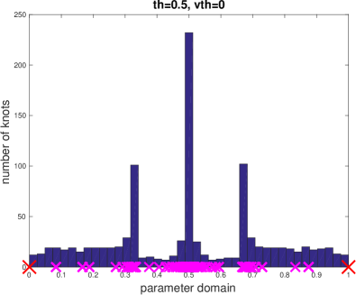
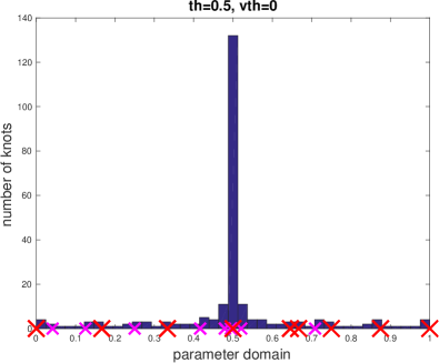
\psfrag{number of knots N}[c][c]{\small number of knots $N$}\psfrag{number of knots}[c][c]{\small number of knots}\psfrag{parameter domain}[c][c]{\small parameter domain}\psfrag{error estimator}[c][c]{\small error estimator}\psfrag{O(47)}[c][c]{\tiny$\mathcal{O}(N^{-4/7})$}\psfrag{O(52)}[c][c]{\tiny$\mathcal{O}(N^{-5/2})$}\psfrag{th=0.5, vth=0}[c][c]{\small$\theta=0.5,\vartheta=0$}\psfrag{th=0.5, vth=0.1}[c][c]{\small$\theta=0.5,\vartheta=0.1$}\psfrag{th=0.5, vth=1}[c][c]{\small$\theta=0.5,\vartheta=1$}\psfrag{ th=1, vth=0}[c][c]{\tiny$\theta=1,\vartheta=0$}\psfrag{ th=0.5, vth=0}[c][c]{\tiny$\theta=0.5,\vartheta=0$}\psfrag{ th=0.5, vth=0.1}[c][c]{\tiny$\theta=0.5,\vartheta=0.1$}\psfrag{ th=0.5, vth=1}[c][c]{\tiny$\theta=0.5,\vartheta=1$}\includegraphics[width=205.97214pt,clip={true}]{figures/hist_hyper_1geo_pacmanp_2vartheta_0.1}

\psfrag{number of knots N}[c][c]{\small number of knots $N$}\psfrag{number of knots}[c][c]{\small number of knots}\psfrag{parameter domain}[c][c]{\small parameter domain}\psfrag{error estimator}[c][c]{\small error estimator}\psfrag{O(47)}[c][c]{\tiny$\mathcal{O}(N^{-4/7})$}\psfrag{O(52)}[c][c]{\tiny$\mathcal{O}(N^{-5/2})$}\psfrag{th=0.5, vth=0}[c][c]{\small$\theta=0.5,\vartheta=0$}\psfrag{th=0.5, vth=0.1}[c][c]{\small$\theta=0.5,\vartheta=0.1$}\psfrag{th=0.5, vth=1}[c][c]{\small$\theta=0.5,\vartheta=1$}\psfrag{ th=1, vth=0}[c][c]{\tiny$\theta=1,\vartheta=0$}\psfrag{ th=0.5, vth=0}[c][c]{\tiny$\theta=0.5,\vartheta=0$}\psfrag{ th=0.5, vth=0.1}[c][c]{\tiny$\theta=0.5,\vartheta=0.1$}\psfrag{ th=0.5, vth=1}[c][c]{\tiny$\theta=0.5,\vartheta=1$}\includegraphics[width=205.97214pt,clip={true}]{figures/hist_hyper_1geo_pacmanp_2vartheta_1}

Figure 5.3. Hyper-singular integral equation on pacman (Section 5.1). Convergence plot of the error estimators $\eta_{\ell}$ and histograms of the knots $\widehat{\mathcal{K}}_{\ell}$ of the last refinement step. Knots with multiplicity 3 are highlighted by a red cross, knots with multiplicity 2 by a smaller magenta cross.

5.2. Weakly-singular integral equation on pacman

In Figure 5.4, the corresponding error estimators $\eta_{\ell}$ are plotted. Since the solution lacks regularity, uniform refinement leads to the suboptimal rate $\mathcal{O}(N^{-4/7})$, whereas adaptive refinement leads to the optimal rate $\mathcal{O}(N^{-3/2-p})=\mathcal{O}(N^{-7/2})$. For $\vartheta=1$, the corresponding multiplicative constant is clearly larger than for $\vartheta\in\{0,0.1\}$. A possible explanation is that $\vartheta=1$ results in too few multiplicity increases. Indeed, the histograms in Figure 5.3 of the knots $\widehat{\mathcal{K}}_{\ell}$ from the last refinement step indicate that $\vartheta\in\{0,0.1\}$ leads to full multiplicity of the knots $1/3$ and $2/3$, which is exactly where the solution $\phi\circ\gamma$ on the parameter domain (depicted in Figure 5.2) has jumps. In contrast, the choice $\vartheta=1$ compensates the lacking regularity at these points by $h$-refinement; see also [FGHP16, Section 3]. Again, $\vartheta\in\{0.1,1\}$ give a more accurate information on the regularity of the solution.

\psfrag{number of knots N}[c][c]{\small number of knots $N$}\psfrag{number of knots}[c][c]{\small number of knots}\psfrag{parameter domain}[c][c]{\small parameter domain}\psfrag{error estimator}[c][c]{\small error estimator}\psfrag{O(47)}[c][c]{\tiny$\mathcal{O}(N^{-4/7})$}\psfrag{O(72)}[c][c]{\tiny$\mathcal{O}(N^{-7/2})$}\psfrag{th=0.5, vth=0}[c][c]{\small$\theta=0.5,\vartheta=0$}\psfrag{th=0.5, vth=0.1}[c][c]{\small$\theta=0.5,\vartheta=0.1$}\psfrag{th=0.5, vth=1}[c][c]{\small$\theta=0.5,\vartheta=1$}\psfrag{ th=1, vth=0}[c][c]{\tiny$\theta=1,\vartheta=0$}\psfrag{ th=0.5, vth=0}[c][c]{\tiny$\theta=0.5,\vartheta=0$}\psfrag{ th=0.5, vth=0.1}[c][c]{\tiny$\theta=0.5,\vartheta=0.1$}\psfrag{ th=0.5, vth=1}[c][c]{\tiny$\theta=0.5,\vartheta=1$}\includegraphics[width=205.97214pt,clip={true}]{figures/conv_hyper_0geo_pacmanp_2}

\psfrag{number of knots N}[c][c]{\small number of knots $N$}\psfrag{number of knots}[c][c]{\small number of knots}\psfrag{parameter domain}[c][c]{\small parameter domain}\psfrag{error estimator}[c][c]{\small error estimator}\psfrag{O(47)}[c][c]{\tiny$\mathcal{O}(N^{-4/7})$}\psfrag{O(72)}[c][c]{\tiny$\mathcal{O}(N^{-7/2})$}\psfrag{th=0.5, vth=0}[c][c]{\small$\theta=0.5,\vartheta=0$}\psfrag{th=0.5, vth=0.1}[c][c]{\small$\theta=0.5,\vartheta=0.1$}\psfrag{th=0.5, vth=1}[c][c]{\small$\theta=0.5,\vartheta=1$}\psfrag{ th=1, vth=0}[c][c]{\tiny$\theta=1,\vartheta=0$}\psfrag{ th=0.5, vth=0}[c][c]{\tiny$\theta=0.5,\vartheta=0$}\psfrag{ th=0.5, vth=0.1}[c][c]{\tiny$\theta=0.5,\vartheta=0.1$}\psfrag{ th=0.5, vth=1}[c][c]{\tiny$\theta=0.5,\vartheta=1$}\includegraphics[width=205.97214pt,clip={true}]{figures/hist_hyper_0geo_pacmanp_2vartheta_0.1}

\psfrag{number of knots N}[c][c]{\small number of knots $N$}\psfrag{number of knots}[c][c]{\small number of knots}\psfrag{parameter domain}[c][c]{\small parameter domain}\psfrag{error estimator}[c][c]{\small error estimator}\psfrag{O(47)}[c][c]{\tiny$\mathcal{O}(N^{-4/7})$}\psfrag{O(72)}[c][c]{\tiny$\mathcal{O}(N^{-7/2})$}\psfrag{th=0.5, vth=0}[c][c]{\small$\theta=0.5,\vartheta=0$}\psfrag{th=0.5, vth=0.1}[c][c]{\small$\theta=0.5,\vartheta=0.1$}\psfrag{th=0.5, vth=1}[c][c]{\small$\theta=0.5,\vartheta=1$}\psfrag{ th=1, vth=0}[c][c]{\tiny$\theta=1,\vartheta=0$}\psfrag{ th=0.5, vth=0}[c][c]{\tiny$\theta=0.5,\vartheta=0$}\psfrag{ th=0.5, vth=0.1}[c][c]{\tiny$\theta=0.5,\vartheta=0.1$}\psfrag{ th=0.5, vth=1}[c][c]{\tiny$\theta=0.5,\vartheta=1$}\includegraphics[width=205.97214pt,clip={true}]{figures/hist_hyper_0geo_pacmanp_2vartheta_1}

Figure 5.4. Weakly-singular integral equation on pacman (Section 5.2). Convergence plot of the error estimators $\eta_{\ell}$ and histograms of the knots $\widehat{\mathcal{K}}_{\ell}$ of the last refinement step. Knots with multiplicity 3 are highlighted by a red cross, knots with multiplicity 2 by a smaller magenta cross.

5.3. Hyper-singular integral equation on heart

In Figure 5.5, the corresponding error estimators $\eta_{\ell}$ are plotted. Since the Neumann data, which have to be resolved, lack regularity, uniform refinement leads to the suboptimal rate $\mathcal{O}(N^{-2/3})$, whereas adaptive refinement leads to the optimal rate $\mathcal{O}(N^{-1/2-p})=\mathcal{O}(N^{-5/2})$. While the estimator curves look very similar, the choices $\vartheta\in\{0.1,1\}$ (allowing for knot multiplicity decrease) additionally give accurate information on the regularity of the solution; see the histograms in Figure 5.5. Note that the (periodic extension of the) exact solution $u\circ\gamma$ on the parameter domain (depicted in Figure 5.2) is only $C^{0}$ at $0$ resp. $1$, $1/6$, and $5/6$.

\psfrag{number of knots N}[c][c]{\small number of knots $N$}\psfrag{number of knots}[c][c]{\small number of knots}\psfrag{parameter domain}[c][c]{\small parameter domain}\psfrag{error estimator}[c][c]{\small error estimator}\psfrag{O(23)}[c][c]{\tiny$\mathcal{O}(N^{-2/3})$}\psfrag{O(52)}[c][c]{\tiny$\mathcal{O}(N^{-5/2})$}\psfrag{th=0.5, vth=0}[c][c]{\small$\theta=0.5,\vartheta=0$}\psfrag{th=0.5, vth=0.1}[c][c]{\small$\theta=0.5,\vartheta=0.1$}\psfrag{th=0.5, vth=1}[c][c]{\small$\theta=0.5,\vartheta=1$}\psfrag{ th=1, vth=0}[c][c]{\tiny$\theta=1,\vartheta=0$}\psfrag{ th=0.5, vth=0}[c][c]{\tiny$\theta=0.5,\vartheta=0$}\psfrag{ th=0.5, vth=0.1}[c][c]{\tiny$\theta=0.5,\vartheta=0.1$}\psfrag{ th=0.5, vth=1}[c][c]{\tiny$\theta=0.5,\vartheta=1$}\includegraphics[width=205.97214pt,clip={true}]{figures/conv_hyper_1geo_heartp_2}

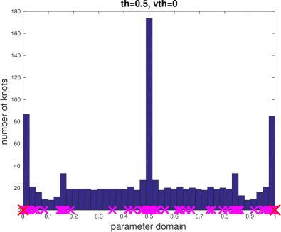
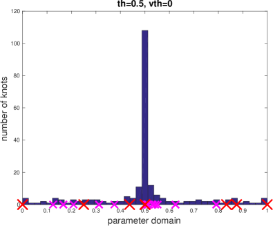
\psfrag{number of knots N}[c][c]{\small number of knots $N$}\psfrag{number of knots}[c][c]{\small number of knots}\psfrag{parameter domain}[c][c]{\small parameter domain}\psfrag{error estimator}[c][c]{\small error estimator}\psfrag{O(23)}[c][c]{\tiny$\mathcal{O}(N^{-2/3})$}\psfrag{O(52)}[c][c]{\tiny$\mathcal{O}(N^{-5/2})$}\psfrag{th=0.5, vth=0}[c][c]{\small$\theta=0.5,\vartheta=0$}\psfrag{th=0.5, vth=0.1}[c][c]{\small$\theta=0.5,\vartheta=0.1$}\psfrag{th=0.5, vth=1}[c][c]{\small$\theta=0.5,\vartheta=1$}\psfrag{ th=1, vth=0}[c][c]{\tiny$\theta=1,\vartheta=0$}\psfrag{ th=0.5, vth=0}[c][c]{\tiny$\theta=0.5,\vartheta=0$}\psfrag{ th=0.5, vth=0.1}[c][c]{\tiny$\theta=0.5,\vartheta=0.1$}\psfrag{ th=0.5, vth=1}[c][c]{\tiny$\theta=0.5,\vartheta=1$}\includegraphics[width=205.97214pt,clip={true}]{figures/hist_hyper_1geo_heartp_2vartheta_0.1}

\psfrag{number of knots N}[c][c]{\small number of knots $N$}\psfrag{number of knots}[c][c]{\small number of knots}\psfrag{parameter domain}[c][c]{\small parameter domain}\psfrag{error estimator}[c][c]{\small error estimator}\psfrag{O(23)}[c][c]{\tiny$\mathcal{O}(N^{-2/3})$}\psfrag{O(52)}[c][c]{\tiny$\mathcal{O}(N^{-5/2})$}\psfrag{th=0.5, vth=0}[c][c]{\small$\theta=0.5,\vartheta=0$}\psfrag{th=0.5, vth=0.1}[c][c]{\small$\theta=0.5,\vartheta=0.1$}\psfrag{th=0.5, vth=1}[c][c]{\small$\theta=0.5,\vartheta=1$}\psfrag{ th=1, vth=0}[c][c]{\tiny$\theta=1,\vartheta=0$}\psfrag{ th=0.5, vth=0}[c][c]{\tiny$\theta=0.5,\vartheta=0$}\psfrag{ th=0.5, vth=0.1}[c][c]{\tiny$\theta=0.5,\vartheta=0.1$}\psfrag{ th=0.5, vth=1}[c][c]{\tiny$\theta=0.5,\vartheta=1$}\includegraphics[width=205.97214pt,clip={true}]{figures/hist_hyper_1geo_heartp_2vartheta_1}

Figure 5.5. Hyper-singular integral equation on heart (Section 5.3). Convergence plot of the error estimators $\eta_{\ell}$ and histograms of the knots $\widehat{\mathcal{K}}_{\ell}$ of the last refinement step. Knots with multiplicity 3 are highlighted by a red cross, knots with multiplicity 2 by a smaller magenta cross.

5.4. Weakly-singular integral equation on heart

In Figure 5.4, the corresponding error estimators $\eta_{\ell}$ are plotted. Since the solution lacks regularity, uniform refinement leads to the suboptimal rate $\mathcal{O}(N^{-2/3})$, whereas adaptive refinement leads to the optimal rate $\mathcal{O}(N^{-3/2-p})=\mathcal{O}(N^{-7/2})$. Figure 5.3 further provides histograms of the knots $\widehat{\mathcal{K}}_{\ell}$ from the last refinement step. Overall, we observe a similar behavior as in Section 5.2. Note that the (periodic extension of the) exact solution $\phi\circ\gamma$ on the parameter domain (depicted in Figure 5.2) is only $C^{0}$ at $0$ resp. $1$, $1/6$, and $5/6$.

\psfrag{number of knots N}[c][c]{\small number of knots $N$}\psfrag{number of knots}[c][c]{\small number of knots}\psfrag{parameter domain}[c][c]{\small parameter domain}\psfrag{error estimator}[c][c]{\small error estimator}\psfrag{O(23)}[c][c]{\tiny$\mathcal{O}(N^{-2/3})$}\psfrag{O(72)}[c][c]{\tiny$\mathcal{O}(N^{-7/2})$}\psfrag{th=0.5, vth=0}[c][c]{\small$\theta=0.5,\vartheta=0$}\psfrag{th=0.5, vth=0.1}[c][c]{\small$\theta=0.5,\vartheta=0.1$}\psfrag{th=0.5, vth=1}[c][c]{\small$\theta=0.5,\vartheta=1$}\psfrag{ th=1, vth=0}[c][c]{\tiny$\theta=1,\vartheta=0$}\psfrag{ th=0.5, vth=0}[c][c]{\tiny$\theta=0.5,\vartheta=0$}\psfrag{ th=0.5, vth=0.1}[c][c]{\tiny$\theta=0.5,\vartheta=0.1$}\psfrag{ th=0.5, vth=1}[c][c]{\tiny$\theta=0.5,\vartheta=1$}\includegraphics[width=205.97214pt,clip={true}]{figures/conv_hyper_0geo_heartp_2}

\psfrag{number of knots N}[c][c]{\small number of knots $N$}\psfrag{number of knots}[c][c]{\small number of knots}\psfrag{parameter domain}[c][c]{\small parameter domain}\psfrag{error estimator}[c][c]{\small error estimator}\psfrag{O(23)}[c][c]{\tiny$\mathcal{O}(N^{-2/3})$}\psfrag{O(72)}[c][c]{\tiny$\mathcal{O}(N^{-7/2})$}\psfrag{th=0.5, vth=0}[c][c]{\small$\theta=0.5,\vartheta=0$}\psfrag{th=0.5, vth=0.1}[c][c]{\small$\theta=0.5,\vartheta=0.1$}\psfrag{th=0.5, vth=1}[c][c]{\small$\theta=0.5,\vartheta=1$}\psfrag{ th=1, vth=0}[c][c]{\tiny$\theta=1,\vartheta=0$}\psfrag{ th=0.5, vth=0}[c][c]{\tiny$\theta=0.5,\vartheta=0$}\psfrag{ th=0.5, vth=0.1}[c][c]{\tiny$\theta=0.5,\vartheta=0.1$}\psfrag{ th=0.5, vth=1}[c][c]{\tiny$\theta=0.5,\vartheta=1$}\includegraphics[width=205.97214pt,clip={true}]{figures/hist_hyper_0geo_heartp_2vartheta_0.1}

\psfrag{number of knots N}[c][c]{\small number of knots $N$}\psfrag{number of knots}[c][c]{\small number of knots}\psfrag{parameter domain}[c][c]{\small parameter domain}\psfrag{error estimator}[c][c]{\small error estimator}\psfrag{O(23)}[c][c]{\tiny$\mathcal{O}(N^{-2/3})$}\psfrag{O(72)}[c][c]{\tiny$\mathcal{O}(N^{-7/2})$}\psfrag{th=0.5, vth=0}[c][c]{\small$\theta=0.5,\vartheta=0$}\psfrag{th=0.5, vth=0.1}[c][c]{\small$\theta=0.5,\vartheta=0.1$}\psfrag{th=0.5, vth=1}[c][c]{\small$\theta=0.5,\vartheta=1$}\psfrag{ th=1, vth=0}[c][c]{\tiny$\theta=1,\vartheta=0$}\psfrag{ th=0.5, vth=0}[c][c]{\tiny$\theta=0.5,\vartheta=0$}\psfrag{ th=0.5, vth=0.1}[c][c]{\tiny$\theta=0.5,\vartheta=0.1$}\psfrag{ th=0.5, vth=1}[c][c]{\tiny$\theta=0.5,\vartheta=1$}\includegraphics[width=205.97214pt,clip={true}]{figures/hist_hyper_0geo_heartp_2vartheta_1}

Figure 5.6. Weakly-singular integral equation on heart (Section 5.4). Convergence plot of the error estimators $\eta_{\ell}$ and histograms of the knots $\widehat{\mathcal{K}}_{\ell}$ of the last refinement step. Knots with multiplicity 3 are highlighted by a red cross, knots with multiplicity 2 by a smaller magenta cross.

Appendix A Weakly-singular integral equation

In this appendix, we consider the weakly-singular integral equation

$$\mathfrak{V}\phi=(1/2+\mathfrak{K})u\quad\text{with given }u\in H^{1/2}(\Gamma),$$ (A.1)

which is equivalent to the Laplace–Dirichlet problem

$$-\Delta P=0\text{ in }\Omega\quad\text{subject to Dirichlet boundary conditions}\quad P|_{\Gamma}=u\text{ on }\Gamma=\partial\Omega,$$ (A.2)

where $\phi=\partial P/\partial\nu$ is the normal derivative of the sought potential $P$.

A.1. Functional analytic setting

The weakly-singular integral equation (A.1) employs the single-layer operator $\mathfrak{V}$ as well as the double-layer operator $\mathfrak{K}^{\prime}$. These have the boundary integral representations

$$\mathfrak{V}\phi(x)=\int_{\Gamma}\phi(y)G(x,y)\,dy\quad\text{and}\quad\mathfrak{K}u(x)=\int_{\Gamma}u(y)\frac{\partial_{y}}{\partial\nu(y)}G(x,y)\,dy$$ (A.3)

for smooth densities $\phi,u:\Gamma\to{\mathbb{R}}$.

For $0\leq\sigma\leq 1$, the single-layer operator ${\mathfrak{V}}:H^{\sigma-1}(\Gamma)\to H^{\sigma}(\Gamma)$ and the double-layer operator $\mathfrak{K}:H^{\sigma}(\Gamma)\to H^{\sigma}(\Gamma)$ are well-defined, linear, and continuous.

For $\sigma=1/2$, ${\mathfrak{V}}:H^{-1/2}(\Gamma)\to H^{1/2}(\Gamma)$ is symmetric and elliptic under the assumption that ${\rm diam}(\Omega)<1$, which can always be achieved by scaling $\Omega$. In particular,

$$\langle\phi\,,\,\psi\rangle_{{\mathfrak{V}}}:=\langle{\mathfrak{V}}\phi\,,\,\psi\rangle_{\Gamma}$$ (A.4)

defines an equivalent scalar product on $H^{-1/2}(\Gamma)$ with corresponding norm $||\cdot||_{{\mathfrak{V}}}$. With this notation, the strong form (A.1) with data $u\in H^{1/2}(\Gamma)$ is equivalently stated by

$$\langle\phi\,,\,\psi\rangle_{{\mathfrak{V}}}=\langle(1/2+\mathfrak{K})u\,,\,\psi\rangle_{\Gamma}\quad\text{for all }\psi\in H^{-1/2}(\Gamma).$$ (A.5)

Therefore, the Lax-Milgram lemma applies and proves that (A.5) resp.  (A.1) admits a unique solution $\phi\in H^{-1/2}(\Gamma)$. Details are found, e.g., in [HW08, McL00, SS11, Ste08].

A.2. IGABEM discretization

As refinement algorithm for the boundary meshes, we use Algorithm 2.1, where the multiplicity of the knots in step (iii) is now increased up to $p+1$ (instead of $p$), allowing for discontinuities at the nodes. The set $\mathbb{K}$ now denotes the set of all possible knot vectors that can be generated with this modified refinement algorithm starting from an initial knot vector ${\mathcal{K}}_{0}$ as in Section 2.5, where each knot in ${\mathcal{K}}_{0}$ might have multiplicity up to $p+1$. Further, we do no longer require the restriction $w_{0,1-p}=w_{0,N_{0}-p}$ for the weights. For ${\mathcal{K}}_{\bullet}\in\mathbb{K}$, we define the corresponding ansatz space as

$${\mathcal{X}}_{\bullet}:={\mathcal{S}}^{p}({\mathcal{K}}_{\bullet},\mathcal{W}_{\bullet})={\rm span}\big{\{}R_{\bullet,i,p}\,:\,i=1-p,\dots,N_{\bullet}-p\big{\}}$$ (A.6)

and the Galerkin approximation $\Phi_{\bullet}\in{\mathcal{X}}_{\bullet}$ of $\phi$ via

$$\langle\Phi_{\bullet}\,,\,\Psi_{\bullet}\rangle_{{\mathfrak{V}}}=\langle g_{\bullet}\,,\,\Psi_{\bullet}\rangle_{\Gamma}\,\text{ for all }\Psi_{\bullet}\in{\mathcal{X}}_{\bullet},\quad\text{where }g_{\bullet}:=(1/2+\mathfrak{K})u_{\bullet}.$$ (A.7)

Here, we define $u_{\bullet}:=P_{\bullet}\phi$, where $P_{\bullet}$ is either the identity or the Scott–Zhang operator of Section 4.3 onto the space of (transformed) continuous piecewise polynomials ${\mathcal{P}}^{p}({\mathcal{Q}}_{\bullet})\cap C^{0}(\Gamma)$.

In order to employ the weighted-residual error estimator (plus oscillations)

$$\eta_{\bullet}(z)^{2}:=\|h_{\bullet}^{1/2}\partial_{\Gamma}(g_{\bullet}-\mathfrak{V}\Phi_{\bullet})\|_{L^{2}(\pi_{\bullet}(z))}^{2}+\|h_{\bullet}^{1/2}\partial_{\Gamma}(u-u_{\bullet})\|_{L^{2}(\pi_{\bullet}(z))}^{2}\quad\text{for all }z\in{\mathcal{N}}_{\bullet},$$ (A.8)

we require the additional regularity $u\in H^{1}(\Gamma)$. Moreover, we define

$$\mu_{\bullet}(z):=\|h_{\bullet}^{1/2}(1-I_{\bullet\ominus 1})\Phi_{\bullet}\|_{L^{2}(\pi_{\bullet}^{2p+1}(z))}\text{ for all }z\in{\mathcal{N}}_{\bullet},$$ (A.9)

where $I_{\bullet}$ is now the Scott–Zhang operator onto ${\mathcal{X}}_{\bullet}$ defined in [BdVBSV14, Section 3.1.2].

With these definitions, Algorithm 3.1 is also well-defined for the weakly-singular case. As already mentioned in Remark 3.2 (b), the choice $\vartheta=0$ and $\mathcal{M}_{\ell}^{-}=\emptyset$ leads to no multiplicity decreases and then the adaptive algorithm coincides with the one from [FGHP16] if $u_{\bullet}:=u$. For the latter, linear convergence at optimal rate has already been proved in our earlier work [FGHP17]. Theorem 3.3 holds accordingly in the weakly-singular case and thus generalizes [FGHP17]. We will briefly sketch the proof in the remainder of this appendix.

A.3. Reliability and efficiency

Reliability, i.e., $\|\phi-\Phi_{\bullet}\|_{H^{-1/2}(\Gamma)}\lesssim\eta_{\bullet}$ is already stated in [FGHP16, Theorem 4.4]. Efficiency, i.e., $\eta_{\bullet}\lesssim\|h_{\bullet}^{1/2}(\phi-\Phi_{\bullet})\|_{L^{2}(\Gamma)}+\|h_{\bullet}^{-1/2}(g-g_{\bullet})\|_{L^{2}(\Gamma)}$ follows as in [AFF⁺17, Corollary 3.3], which proves the assertion for standard BEM.

A.4. Linear and optimal convergence

Linear convergence (3.11) at optimal rate (3.12) (with similarly defined approximability constant $\|\phi\|_{\mathbb{A}_{s}}$) follows again from the axioms of adaptivity. Stability (E1) follows exactly as the corresponding version [FGHP17, Lemma 5.1]. The main argument is the inverse estimate $\|h_{\bullet}^{1/2}\partial_{\Gamma}({\mathfrak{V}}\Psi_{\bullet})\|_{L^{2}(\Gamma)}\lesssim\|\Psi_{\bullet}\|_{H^{-1/2}(\Gamma)}$ of [FGHP17, Proposition 4.1] for (transformed) rational splines $\Psi_{\bullet}\in{\mathcal{X}}_{\bullet}$. Reduction (E2) follows as in [FGHP17, Lemma 4.4]. It is proved via the same inverse estimate together with the contraction property (4.2) of $\widetilde{h}_{\pi_{\bullet}(z)}$. Details are also found in [Gan17, Section 5.8.4 resp. Section 5.8.5]. We have already proved discrete reliability in [FGHP17, Lemma 5.2]; see also [Gan17, Section 5.8.7] for details. The proof of quasi-orthogonality (E4) is almost identical as for the hyper-singular case in Section 4.10. The son estimate is verified as in Section 4.11 and the closure estimate (R2) as well as the overlay property (R3) are already found in [FGHP17, Proposition 2.2].

A.5. Approximability constants

Similarly as in (3.13), we have that $\|\phi\|_{\mathbb{A}_{s}^{1}}\lesssim\|\phi\|_{\mathbb{A}_{s}}\leq\min\{\|\phi\|_{\mathbb{A}_{s}^{1}},\|\phi\|_{\mathbb{A}_{s}^{p+1}}\}\lesssim\|\phi\|_{\mathbb{A}_{s}^{1}}$, where the approximability constants are defined analogously as in Section 3.3. The proof follows along the lines of Section 4.15.

Appendix B Indirect BEM

B.1. Hyper-singular case

Theorem 3.3 remains valid if, instead of (1.1), one considers the indirect integral formulation

$$\mathfrak{W}u=\phi\quad\text{with given }\phi\in H_{0}^{-1/2}(\Gamma),$$ (B.1)

where the function $\phi$ is again approximated via $\phi_{\bullet}$ as in Section 2.8. Indeed, the proof becomes even simpler due to the absence of the operator $\mathfrak{K}^{\prime}$.

B.2. Weakly-singular case

Similarly, one can consider

$$\mathfrak{V}\phi=u\quad\text{with given }u\in H^{1/2}(\Gamma)$$ (B.2)

instead of (A.1), where $u$ is approximated as in Appendix A, and the results of Appendix A remain valid. Again, the proof even simplifies due to the absence of the operator $\mathfrak{K}$.

Appendix C Slit problems

In contrast to before, let now $\Gamma\subsetneqq\partial\Omega$ be a connected proper subset of the boundary $\partial\Omega$ with parametrization $\gamma:[a,b]\to\Gamma$. Let $E_{0}(\cdot)$ denote the extension of a function on $\Gamma$ by zero onto the whole boundary.

C.1. Hyper-singular case

We consider the slit problem

$$(\mathfrak{W}E_{0}u)|_{\Gamma}=\phi\quad\text{with given }\phi\in H^{-1/2}(\Gamma).$$ (C.1)

Here, $H^{-1/2}(\Gamma)$ denotes the dual space of $\widetilde{H}^{1/2}(\Gamma)=[L^{2}(\Gamma),\widetilde{H}^{1}(\Gamma)]_{1/2}$, where $\widetilde{H}^{1}(\Gamma)$ is the set of all $H^{1}(\Gamma)$ functions with vanishing trace on the relative boundary $\partial\Gamma$. The operator $(\mathfrak{W}E_{0}(\cdot))|_{\Gamma}:\widetilde{H}^{1/2}(\Gamma)\to H^{-1/2}(\Gamma)$ is linear, continuous, and elliptic. Let $\mathbb{K}$ now denote the set of all knot vectors that can be generated via Algorithm 2.1 from an initial knot vector ${\mathcal{K}}_{0}$ on $\Gamma$. For ${\mathcal{K}}_{\bullet}\in\mathbb{K}$ and corresponding weights $\mathcal{W}_{\bullet}$ as in Section 2.8 without the restriction $w_{\bullet,1-p}=w_{\bullet,N_{\bullet}-p}$, we define the ansatz space

$${\mathcal{X}}_{\bullet}:=\big{\{}V\,:\,V\circ\gamma\in\widehat{\mathcal{S}}(\widehat{\mathcal{K}}_{\bullet},\mathcal{W}_{\bullet})\wedge 0=V(\gamma(a+))=V(\gamma(b-))\big{\}}\subset\widetilde{H}^{1}(\Gamma).$$ (C.2)

Moreover, we define the corresponding Scott–Zhang operator $J_{\bullet}:L^{2}(\Gamma)\to{\mathcal{X}}_{\bullet}$ similarly as in Section 4.3 via

$$J_{\bullet}v:=\sum_{i=2-p}^{N_{\bullet}-p-1}\Big{(}\int_{a}^{b}\widehat{R}_{\bullet,i,p}^{*}(v\circ\gamma)\,dt\Big{)}R_{\bullet,i,p}.$$ (C.3)

Replacing the spaces $H^{\sigma}(\Gamma)$ and $H^{1}(\Gamma)$ by $\widetilde{H}^{\sigma}(\Gamma)$ and $\widetilde{H}^{1}(\Gamma)$, Proposition 4.3 is also satisfied in this case, where the proof additionally employs the Friedrichs inequality. If we approximate $\phi$ as in Section 2.8, Theorem 3.3 holds accordingly. The proof follows along the same lines.

C.2. Weakly-singular case

We consider the slit problem

$$(\mathfrak{V}E_{0}\phi)|_{\Gamma}=u\quad\text{with}\quad u\in H^{1/2}(\Gamma),$$ (C.4)

where $H^{1/2}(\Gamma)=[L^{2}(\Gamma),H^{1}(\Gamma)]_{1/2}$. The dual space of the latter is denoted by $\widetilde{H}^{-1/2}(\Gamma)$. The operator $(\mathfrak{V}E_{0}(\cdot))|_{\Gamma}:\widetilde{H}^{-1/2}(\Gamma)\to H^{1/2}(\Gamma)$ is linear, continuous, and elliptic provided that ${\rm diam}(\Omega)<1$. An adaptive IGABEM can be formulated as in Appendix A. Without multiplicity decrease and oscillation terms, it coincides with the algorithm from [FGHP16], which converges linearly at optimal rate according to [FGHP17]. For the generalized version, one can prove the same results as in Appendix A.

Acknowledgement.

The authors are supported by the Austrian Science Fund (FWF) through the research projects Optimal isogeometric boundary element method (grant P29096) and Optimal adaptivity for BEM and FEM-BEM coupling (grant P27005), the doctoral school Dissipation and dispersion in nonlinear PDEs (grant W1245), and the special research program Taming complexity in PDE systems (grant SFB F65).

References

- [ACD+18] Alessandra Aimi, Francesco Calabrò, Mauro Diligenti, Maria L. Sampoli, Giancarlo Sangalli, and Alessandra Sestini. Efficient assembly based on B-spline tailored quadrature rules for the IgA-SGBEM. Comput. Methods Appl. Mech. Engrg., 331:327–342, 2018.
- [ADSS16] Alessandra Aimi, Mauro Diligenti, Maria L. Sampoli, and Alessandra Sestini. Isogemetric analysis and symmetric Galerkin BEM: A 2D numerical study. Appl. Math. Comput., 272:173–186, 2016.
- [AFF+13] Markus Aurada, Michael Feischl, Thomas Führer, Michael Karkulik, and Dirk Praetorius. Efficiency and optimality of some weighted-residual error estimator for adaptive 2D boundary element methods. Comput. Methods Appl. Math., 13(3):305–332, 2013.
- [AFF+15] Markus Aurada, Michael Feischl, Thomas Führer, Michael Karkulik, and Dirk Praetorius. Energy norm based error estimators for adaptive BEM for hypersingular integral equations. Appl. Numer. Math., 95:250–270, 2015.
- [AFF+17] Markus Aurada, Michael Feischl, Thomas Führer, Michael Karkulik, Jens Markus Melenk, and Dirk Praetorius. Local inverse estimates for non-local boundary integral operators. Math. Comp., 86:2651–2686, 2017.
- [BdVBSV14] Lourenco Beirão da Veiga, Annalisa Buffa, Giancarlo Sangalli, and Rafael Vázquez. Mathematical analysis of variational isogeometric methods. Acta Numer., 23:157–287, 2014.
- [BG16] Annalisa Buffa and Carlotta Giannelli. Adaptive isogeometric methods with hierarchical splines: error estimator and convergence. Math. Models Methods Appl. Sci., 26(1):1–25, 2016.
- [BG17] Annalisa Buffa and Carlotta Giannelli. Adaptive isogeometric methods with hierarchical splines: optimality and convergence rates. Math. Models Methods Appl. Sci., 27(14):2781–2802, 2017.
- [BL76] Jöran Bergh and Jörgen Löfström. Interpolation spaces. An introduction. Berlin, 1976.
- [Car97] Carsten Carstensen. An a posteriori error estimate for a first-kind integral equation. Math. Comp., 66(217):139–155, 1997.
- [CFPP14] Carsten Carstensen, Michael Feischl, Marcus Page, and Dirk Praetorius. Axioms of adaptivity. Comput. Math. Appl., 67(6):1195–1253, 2014.
- [CHB09] J. Austin Cottrell, Thomas J. R. Hughes, and Yuri Bazilevs. Isogeometric analysis. John Wiley & Sons, Ltd., Chichester, 2009.
- [CMPS04] Carsten Carstensen, Matthias Maischak, Dirk Praetorius, and Ernst P. Stephan. Residual-based a posteriori error estimate for hypersingular equation on surfaces. Numer. Math., 97(3):397–425, 2004.
- [CP06] Carsten Carstensen and Dirk Praetorius. Averaging techniques for the effective numerical solution of symm’s integral equation of the first kind. SIAM J. Sci. Comp., 27(4):1226–1260, 2006.
- [CS95] Carsten Carstensen and Ernst P. Stephan. Adaptive coupling of boundary elements and finite elements. RAIRO Modél. Math. Anal. Numér., 29(7):779–817, 1995.
- [dB86] Carl de Boor. B (asic)-spline basics. Mathematics Research Center, University of Wisconsin-Madison, 1986.
- [DHK+18] Jürgen Dölz, Helmut Harbrecht, Stefan Kurz, Sebastian Schöps, and Felix Wolf. A fast isogeometric BEM for the three dimensional Laplace- and Helmholtz problems. Comput. Methods Appl. Mech. Engrg., 330:83–101, 2018.
- [DHP16] Jürgen Dölz, Helmut Harbrecht, and Michael Peters. An interpolation-based fast multipole method for higher-order boundary elements on parametric surfaces. Internat. J. Numer. Methods Engrg., 108(13):1705–1728, 2016.
- [DKSW18] Jürgen Dölz, Stefan Kurz, Sebastian Schöps, and Felix Wolf. Isogeometric boundary elements in electromagnetism: Rigorous analysis, fast methods, and examples. arXiv preprint, 1807.03097, 2018.
- [Fae00] Birgit Faermann. Localization of the Aronszajn-Slobodeckij norm and application to adaptive boundary element methods. I. The two-dimensional case. IMA J. Numer. Anal., 20(2):203–234, 2000.
- [FFK+14] Michael Feischl, Thomas Führer, Michael Karkulik, Jens Markus Melenk, and Dirk Praetorius. Quasi-optimal convergence rates for adaptive boundary element methods with data approximation, part I: weakly-singular integral equation. Calcolo, 51(4):531–562, 2014.
- [FFK+15] Michael Feischl, Thomas Führer, Michael Karkulik, J. Markus Melenk, and Dirk Praetorius. Quasi-optimal convergence rates for adaptive boundary element methods with data approximation. Part II: Hyper-singular integral equation. Electron. Trans. Numer. Anal., 44:153–176, 2015.
- [FGHP16] Michael Feischl, Gregor Gantner, Alexander Haberl, and Dirk Praetorius. Adaptive 2D IGA boundary element methods. Eng. Anal. Bound. Elem., 62:141–153, 2016.
- [FGHP17] Michael Feischl, Gregor Gantner, Alexander Haberl, and Dirk Praetorius. Optimal convergence for adaptive IGA boundary element methods for weakly-singular integral equations. Numer. Math., 136(1):147–182, 2017.
- [FGK+18] Antonella Falini, Carlotta Giannelli, Tadej Kanduč, Maria L. Sampoli, and Alessandra Sestini. An adaptive IgA-BEM with hierarchical B-splines based on quasi-interpolation quadrature schemes. Internat. J. Numer. Methods Engrg., 2018.
- [FGP15] Michael Feischl, Gregor Gantner, and Dirk Praetorius. Reliable and efficient a posteriori error estimation for adaptive IGA boundary element methods for weakly-singular integral equations. Comput. Methods Appl. Mech. Engrg., 290:362–386, 2015.
- [FGPS18] Thomas Führer, Gregor Gantner, Dirk Praetorius, and Stefan Schimanko. Optimal additive Schwarz preconditioning for adaptive 2D IGA boundary element methods. arXiv preprint, 1808.04585, 2018.
- [FKMP13] Michael Feischl, Michael Karkulik, Jens M. Melenk, and Dirk Praetorius. Quasi-optimal convergence rate for an adaptive boundary element method. SIAM J. Numer. Anal., 51(2):1327–1348, 2013.
- [Gan13] Tsogtorel Gantumur. Adaptive boundary element methods with convergence rates. Numer. Math., 124:471–516, 2013.
- [Gan14] Gregor Gantner. Adaptive isogeometric BEM. Master’s thesis, TU Wien, 2014.
- [Gan17] Gregor Gantner. Optimal adaptivity for splines in finite and boundary element methods. PhD thesis, TU Wien, 2017.
- [GHP17] Gregor Gantner, Daniel Haberlik, and Dirk Praetorius. Adaptive IGAFEM with optimal convergence rates: hierarchical B-splines. Math. Models Methods Appl. Sci., 27(14):2631–2674, 2017.
- [GHS05] Ivan G. Graham, Wolfgang Hackbusch, and Stefan A. Sauter. Finite elements on degenerate meshes: inverse-type inequalities and applications. IMA J. Numer. Anal., 25(2):379–407, 2005.
- [HAD14] Luca Heltai, Marino Arroyo, and Antonio DeSimone. Nonsingular isogeometric boundary element method for Stokes flows in 3D. Comput. Methods Appl. Mech. Engrg., 268:514–539, 2014.
- [HCB05] Thomas J. R. Hughes, J. Austin Cottrell, and Yuri Bazilevs. Isogeometric analysis: CAD, finite elements, NURBS, exact geometry and mesh refinement. Comput. Methods Appl. Mech. Engrg., 194(39-41):4135–4195, 2005.
- [HR10] Helmut Harbrecht and Maharavo Randrianarivony. From computer aided design to wavelet BEM. Comput. Vis. Sci., 13(2):69–82, 2010.
- [HW08] George C. Hsiao and Wolfgang L. Wendland. Boundary integral equations. Springer, Berlin, 2008.
- [KHZvE17] Sören Keuchel, Nils Christian Hagelstein, Olgierd Zaleski, and Otto von Estorff. Evaluation of hypersingular and nearly singular integrals in the isogeometric boundary element method for acoustics. Comput. Methods Appl. Mech. Engrg., 325:488–504, 2017.
- [McL00] William McLean. Strongly elliptic systems and boundary integral equations. Cambridge University Press, Cambridge, 2000.
- [MZBF15] Benjamin Marussig, Jürgen Zechner, Gernot Beer, and Thomas-Peter Fries. Fast isogeometric boundary element method based on independent field approximation. Comput. Methods Appl. Math., 284:458–488, 2015.
- [NZW+17] B. H. Nguyen, Xiaoying Zhuang, Peter Wriggers, Timon Rabczuk, M. E. Mear, and Han D. Tran. Isogeometric symmetric Galerkin boundary element method for three-dimensional elasticity problems. Comput. Methods Appl. Mech. Engrg., 323:132–150, 2017.
- [PGK+09] Costas Politis, Alexandros I. Ginnis, Panagiotis D. Kaklis, Kostas Belibassakis, and Christian Feurer. An isogeometric BEM for exterior potential-flow problems in the plane. In 2009 SIAM/ACM Joint Conference on Geometric and Physical Modeling, pages 349–354. ACM, 2009.
- [PGKF13] Costas Politis, Alexandros I. Ginnis, Panagiotis D. Kaklis, and Christian Feurer. An isogeometric bem for exterior potential-flow problems in the plane. Comput. Methods Appl. Mech. Engrg., 254:197–221, 2013.
- [PTC13] Michael J. Peake, Jon Trevelyan, and Graham Coates. Extended isogeometric boundary element method (XIBEM) for two-dimensional Helmholtz problems. Comput. Methods Appl. Mech. Engrg., 259:93–102, 2013.
- [SBLT13] Robert N. Simpson, Stéphane P. A. Bordas, Haojie Lian, and Jon Trevelyan. An isogeometric boundary element method for elastostatic analysis: 2D implementation aspects. Comput. & Structures, 118:2–12, 2013.
- [SBTR12] Robert N. Simpson, Stéphane P. A. Bordas, Jon Trevelyan, and Timon Rabczuk. A two-dimensional isogeometric boundary element method for elastostatic analysis. Comput. Methods Appl. Mech. Engrg., 209/212:87–100, 2012.
- [Sch16] Stefan Schimanko. Adaptive isogeometric boundary element method for the hyper-singular integral equation. Master’s thesis, TU Wien, 2016.
- [SS11] Stefan A. Sauter and Christoph Schwab. Boundary element methods. Springer-Verlag, Berlin, 2011.
- [Ste08] Olaf Steinbach. Numerical approximation methods for elliptic boundary value problems. Springer, New York, 2008.
- [TM12] Toru Takahashi and Toshiro Matsumoto. An application of fast multipole method to isogeometric boundary element method for Laplace equation in two dimensions. Eng. Anal. Bound. Elem., 36(12):1766–1775, 2012.