Modulated structures in a Lebwohl-Lasher model with chiral interactions

Abstract

We consider a Lebwohl-Lasher lattice model with nematic directors restricted to point along $p$ planar directions. This $XY$ Lebwohl-Lasher system is the nematic analogue of the standard $p$-state clock model. We then include chiral interactions, and introduce a chiral $p$-state nematic clock model. The statistical problem is formulated as a discrete non-linear map on a Cayley tree. The attractors of this map correspond to the physical solutions deep in the interior of the tree. It is possible to observe uniform and periodic structures, depending on temperature and a parameter of chirality. We find many different chiral nematic phases, and point out the effects of temperature and chirality on the modulation associated with these structures.

Keywords: Chiral nematics; statistical models; phase behavior; Cayley tree

1 Introduction

Competing interactions are the basic mechanism to describe the onset of sequences of modulated phases in many physical systems [1, 2, 3, 4]. In magnetism, the most investigated lattice statistical model to account for the existence of spatially modulated structures is the ANNNI model [5, 6, 7], which is an Ising system with competing ferro and antiferromagnetic interactions between first and second-neighbor spins along an axial direction. The ANNNI model exhibits one of the richest phase diagrams in the literature, with a wealth of modulated structures depending on temperature and on a parameter associated with the ratio between the strengths of the competing couplings. It is remarkable that the modulation associated with these periodic structures displays a nontrivial, staircase-like behavior, as a function of the thermodynamic field parameters [8].

There is an alternative mechanism of competition, which is suggested by an earlier proposal of Dzyaloshinskii and Moriya to explain the modulated structures of helimagnets [9, 10, 11]. According to this Dzyaloshinskii - Moriya (DM) mechanism, in addition to the standard exchange interactions, first-neighbor vector spins along an axis are supposed to interact via chiral couplings. In classical statistical mechanics, it is possible to show that the DM formulation is a generalization of the $p$-state chiral clock (CC) models introduced by Huse [12] and Ostlund [13], with planar vector spin variables along $p$ directions, and the inclusion of chiral interactions between first-neighbors along an axis. These CC systems have been shown to lead to similar complex modulated structures as the ANNNI model. The phase diagrams of the CC models display sequences of many different helical ferromagnetic phases, and a complex behavior of the main wave numbers in terms of temperature [12, 13, 14, 15, 16].

Spatially modulated structures with helical ordering are not exclusive of magnetic systems. In soft-matter physics, simple cholesteric phases in liquid-crystalline compounds provide perhaps the best examples of chiral nematic structures, in which the nematic director exhibits a spatial variation of helical type along a given direction [17]. Many physical aspects of cholesteric nematics can be studied in the framework of the phenomenological approaches, along the lines of the Landau-de Gennes theory, with the inclusion of adequate terms associated with the spatial variation of the nematic director [18, 19].

From the molecular point of view, according to an early work by Goossens [20], the consideration of an induced dipole-quadrupole contribution to the dispersion interactions can give rise to a cholesteric phase. This picture has been extended by some investigators [21] [22], with the formulation of a statistical model, of mean-field type, which might be able to describe the temperature effects in a cholesteric phase. In the calculations of van der Meer and collaborators [21], there is a modulated structure, which is not affected by temperature. Although there is no attempt to draw a global phase diagram, the numerical mean-field calculations of Krutzen and Vertogen [22] point out the possibility of a temperature-dependent pitch if one includes a nematic-twist term in the original pair potential. Along Goossens’s ideas, Lin-Liu and collaborators [23] considered a planar model for the cholesteric phase, which does lead to the description of a temperature sensitive pitch. In these earlier statistical mechanics calculations it is difficult to point out the effects of chirality. Also, there is no attempt to draw a global phase diagram in terms of temperature and a parameter to gauge the strength of chiral interactions. In fact, by means of these earlier calculations, it is not clear to see how thermal fluctuations affect the cholesteric pitch.

The statistical mechanics calculations for the magnetic phase diagrams of the ANNNI and CC models provided the inspiration to carry out the present work. Similar calculations were still missing for the Dzyaloshinskii-Moriya picture of model systems with nematic interactions. We then formulated a $p$-state CC model with head-tail symmetry, and checked the existence of long-period structures in a nematic setting. The main goal of this work is the establishment of qualitative contacts with the description of cholesteric structures in liquid crystals. In this preliminary analysis, calculations have been restricted to the simplest versions of these nematic clock models, which are already sufficient to point out the statistical origin of spatially modulated phases, to draw representative global phase diagrams, and give an indication of the change of the pitch with temperature and model parameters. We remark that it is easy to see that there is a correspondence between the essential terms in the Hamiltonians associated with the $p$-state nematic clock model and of a planar version of Goossen’s proposal, as it has been used by Krutzen and Vertogen [22] and by Lin-Liu and collaborators [23].

This paper is organized as follows. In Section 2, we consider a version of the Lebwohl-Lasher (LL) model [24], with the restriction of the nematic directors to point along a discrete set of directions on the $x-y$ planes. On the basis of this LL model, we define a $p$-state nematic clock model (NC), which is the nematic counterpart of the standard (magnetic) clock models. We then introduce chiral interactions along the axis normal to the $x-y$ planes. In Section 3, we define a $p$-state chiral nematic clock model, which we call CNC model. Also, instead of performing a laborious layer-by-layer mean-field calculation, we formulate the problem on a Cayley tree, and restrict the analysis to the simplest, and nontrivial, chiral nematic model, with just $p=6$ angular directions. The problem is reduced to the investigation of a discrete nonlinear map, whose attractors correspond to physical solutions in the deep interior of large Cayley tree (which is known as a Bethe lattice). It should be remarked that we take full advantage of the geometry of a Cayley tree, which is particularly adequate to describe modulation effects along a radial direction, as it has been pointed out in previous work for the ANNNI and chiral clock models. In Section 4, we further simplify the problem by considering the infinite-coordination (mean-field) limit of a Cayley tree, which is a further simplification, and which is sufficient to illustrate the main features of a chiral nematic model system. We show that the global phase diagram of these systems displays many different chiral nematic phases, and give an illustration to show that these modulated structures exhibit a complex behavior in terms of model parameters. Some conclusions as well an outlook of future work are presented in Section 5.

2 The chiral nematic clock model

We consider pair interactions between nematogenic molecules on the sites of a cubic lattice. In the context of the Maier-Saupe approach to the nematic phase transitions [25, 17], we write the Hamiltonian

$$\mathcal{H}_{MS}=-J\sum_{\left(i,j\right)}\sum_{\mu,\nu}Q_{i}^{\mu\nu}\,Q_{j}^{\mu\nu}=-J\sum_{\left(i,j\right)}\mathbf{Q}_{i}\cdot\mathbf{Q}_{j},$$ (1)

where $J>0$ is a positive energy parameter, the first sum is over pairs of lattice sites, $\mu,\nu$ are Cartesian coordinates, and $\mathbf{Q}_{i}$ is a local traceless quadrupolar tensor.

We now restrict the microscopic nematic directors to the $x-y$ plane. In order to account for the head-tail symmetry of nematic liquid crystals, we write a $2\times 2$ traceless tensor,

$$Q_{\mu\nu}=\frac{1}{2}\left(2n_{\mu}n_{\nu}-\delta_{\mu\nu}\right),$$ (2)

where $\mu,\nu$ are restricted to $x,y$, $\delta_{\mu\nu}$ is the usual Kronecker symbol, and $n_{\mu},n_{\nu}$ are the components of a two-dimensional microscopic nematic director,

$$\overrightarrow{n}=\left(\begin{array}[]{c}\cos\theta\\ \sin\theta\end{array}\right).$$ (3)

We then have the traceless tensor

$$\mathbf{Q}=\frac{1}{2}\left(\begin{array}[]{cc}2\cos^{2}\theta-1&2\cos\theta\sin\theta\\ 2\cos\theta\sin\theta&2\sin^{2}\theta-1\end{array}\right),$$ (4)

where $\theta$ is the angle of the (planar) nematic microscopic director with the $x$ axis.

Given the local director elements,

$$\overrightarrow{n}_{i}=\left(\begin{array}[]{c}\cos\theta_{i}\\ \sin\theta_{i}\end{array}\right),\qquad\overrightarrow{n}_{j}=\left(\begin{array}[]{c}\cos\theta_{j}\\ \sin\theta_{j}\end{array}\right),$$ (5)

and discarding a harmless constant term, it is straightforward to write the Hamiltonian of a nematic clock (NC) model,

$$\mathcal{H}_{NC}=-J\sum_{\left(i,j\right)}\cos^{2}\left(\theta_{i}-\theta_{j}\right),$$ (6)

which is an $XY$ version of the well known Lebwohl-Lasher model (and a nematic analogue of the classical $XY$ spin model of magnetism).

We now assume that chiral effects are mimicked by a rotation of the nematic directors around the $z$ axis (which is the normal direction to the $x-y$ planes). We then write

$$\overrightarrow{n}_{rot}=\left(\begin{array}[]{cc}\cos\Delta&\sin\Delta\\ -\sin\Delta&\cos\Delta\end{array}\right)\left(\begin{array}[]{c}\cos\theta\\ \sin\theta\end{array}\right)=\left(\begin{array}[]{c}\cos\left(\theta-\Delta\right)\\ \sin\left(\theta-\Delta\right)\end{array}\right),$$ (7)

where the angle $\Delta$ is the parameter that gauges chirality. The associated tensor is given by

$$\mathbf{Q}_{rot}=\frac{1}{2}\left(\begin{array}[]{cc}2\cos^{2}\left(\theta-\Delta\right)-1&2\cos\left(\theta-\Delta\right)\sin\left(\theta-\Delta\right)\\ 2\cos\left(\theta-\Delta\right)\sin\left(\theta-\Delta\right)&2\sin^{2}\left(\theta-\Delta\right)-1\end{array}\right).$$ (8)

Therefore, the pair interaction between nematogenic elements at sites $i$ and $j$ along the $z$ direction can be written as

$$\mathbf{Q}_{i}\cdot\mathbf{Q}_{rot,j}=\cos^{2}\left(\theta_{i}-\theta_{j}+\Delta\right)-\frac{1}{2},$$ (9)

which leads to a general form of the Hamiltonian of the chiral nematic clock (CNC) model,

$$\mathcal{H}_{CNC}=-J_{0}\sideset{}{{}^{\perp}}{\sum}_{\left(i,j\right)}\,\cos^{2}\left(\theta_{i}-\theta_{j}\right)-J\sideset{}{{}^{\parallel}}{\sum}_{\left(i,j\right)}\,\left[\cos^{2}\left(\theta_{i}-\theta_{j}+\Delta\right)-\frac{1}{2}\right],$$ (10)

where the first sum is over pair interactions along the $x-y$ planes of the cubic lattice, and the second sum is over pair interactions along the $z$ direction of the lattice. We remark that $J_{0}>0$ and $J_{1}>0$ are energy parameters, and $0<\Delta<2\pi$ is the angular parameter that gauges the degree of chirality.

If we consider just $p$ angular directions, this expression is the natural nematic extension of the well-known $p$-state chiral clock model [12, 14], which has been appropriately generalized to describe chiral nematic-like phases. Also, it is straightforward to notice that, for $p$ even, a clock system with local cosine squared interaction is equivalent to a usual clock model with $p/2$ states. As a result, the CNC model with $p$ even presents the same symmetry properties as CC models [12, 13, 7], which are given by the transformations

$$\begin{split}\Delta&\to\frac{2\pi}{p}-\Delta,\\ \theta_{i}&\to\frac{2\pi}{p}-\theta_{i}.\end{split}$$ (11)

These symmetry relations simplify the analysis of the phase behavior of the model.

3 Restricted-orientation model on a Cayley tree

It is important to take into account that the description of macroscopic nematic structures requires the assumption of a head-tail symmetry of the microscopic states. This assumption suggests that we should restrict the considerations to $p$-state CC models with even values of the integer $p$. However, the simplest case, with $p=4$, does not present complex modulated structures, as we explicitly show in Appendix A.

We then consider a $6$-state model, with a discrete choice of angular variables,

$$\theta\left(k\right)=\frac{\pi}{3}\left(k-1\right),\quad k=1,...,6.$$ (12)

Due to the head-tail symmetry of the nematic systems, the pair of angular variables $\theta\left(1\right)$ and $\theta\left(4\right)$ leads to a single tensor variable, which we call $\mathbf{Q}\left(1\right)$. Also, $\theta\left(2\right)$ and $\theta\left(5\right)$ lead to $\mathbf{Q}\left(2\right)$, and the angular variables $\theta\left(3\right)$ and $\theta\left(6\right)$ lead to $\mathbf{Q}\left(3\right)$. We then use equation (4) to write the microscopic tensor variables,

$$\begin{split}\mathbf{Q}\left(1\right)&=\frac{1}{2}\begin{pmatrix}1&0\\ 0&-1\end{pmatrix},\\ \mathbf{Q}\left(2\right)&=\frac{1}{4}\begin{pmatrix}-1&\sqrt{3}\\ \sqrt{3}&1\end{pmatrix},\\ \mathbf{Q}\left(3\right)&=\frac{1}{4}\begin{pmatrix}-1&-\sqrt{3}\\ -\sqrt{3}&1\end{pmatrix}.\end{split}$$ (13)

In this nematic context, the problem is reduced to the consideration of just these three local tensor states, as schematically represented in Figure 1.

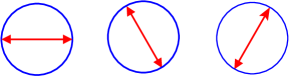
Figure 1: States for the planar Lebwohl-Lasher model. The head-tail symmetry effectively maps a $6$-state vector variable to a $3$-state “nematic clock” variable.

If we assume a set of effective fields along the $z$ direction, it is quite natural to carry out a layer-by-layer mean-field calculation to obtain the phase diagrams associated with the complete model Hamiltonian given by (10). These quite laborious mean-field calculations have indeed been carried out for analyzing the details of the rich phase diagrams of the ANNNI and standard chiral clock models [6]. We now turn to a different and easier approach, which will lead to the same qualitative features of the phase diagrams. Since we are interested in the main overall effects of chirality, it is certainly convenient to take advantage of the radial structure of a Cayley tree. In addition, we perform numerical calculations for the problem in the limit of infinite coordination of a Cayley tree, which is expected to present the same qualitative results of the mean-field calculations.

We now restrict equation (10) to the interactions along the $z$ direction, and write the Hamiltonian

$$\mathcal{H}=-J\sum_{\left(i,j\right)}\,\left[\cos^{2}\left(\theta_{i}-\theta_{j}+\Delta\right)-\frac{1}{2}\right],$$ (14)

for a $6$-state chiral nematic clock model along the branches of a Cayley tree of ramification $r\geq 1$. Similar calculations on a Cayley tree have been carried out for a standard $p$-state chiral clock model [26] and for some analogs of the ANNNI model [27]. It is well known that problems on a Cayley tree can be formulated in terms of discrete non-linear dissipative maps, whose attractors lead to solutions of physical interest. Along the lines of these earlier calculations on a Cayley tree, we write the partial partition function of a tree of $n+1$ generations, $Z_{n+1}\left(i\right)$, in the tensor state $\mathbf{Q}\left(i\right)$, for $i=1,2,3$, at the root site, in terms of the three partial partitions functions, $Z_{n}\left(1\right)$, $Z_{n}\left(2\right)$, and $Z_{n}\left(2\right)$, of the connected trees of the previous $n$ generation. Figure 2 exhibits schematically the branching of a Cayley tree with coordination three, where each vertex presents a nematogenic clock interacting with its next-neighbors, along the tree generations. Physical solutions, in the deep interior of a large tree, correspond to the attractors of the non linear map. This deep interior of a very large tree is known as a Bethe lattice, since the physical solutions are expected to agree with a simple pair or Bethe-Peierls approximation. As we have mentioned, in the limit of infinite coordination (and vanishing interactions), $r\rightarrow\infty$, $J\rightarrow 0$, with $rJ$ fixed, we are supposed to recover the main features of the standard mean-field results [26, 27].

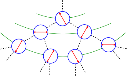
Figure 2: Local structure of the planar Lebwohl-Lasher model on a Cayley tree with coordination three. “Nematic clocks” sit on the vertices of the tree. Interactions (dashed lines) are between next-neighbors along the branches of the tree.

We now adopt a more compact notation, and write a set of three recurrence relations between the partial partition functions of a tree of $n+1$ generations, $Z_{1}^{\prime}=Z_{n+1}\left(1\right)$, $Z_{2}^{\prime}=Z_{n+1}\left(2\right)$, and $Z_{3}^{\prime}=Z_{n+1}\left(3\right)$, and the partition functions of a tree of $n$ generations. Although it demands some algebraic effort, it is not difficult to obtain

$$\begin{split}Z_{1}^{\prime}&=\left[A\,Z_{1}+B\,Z_{2}+C\,Z_{3}\right]^{r},\\ Z_{2}^{\prime}&=\left[C\,Z_{1}+A\,Z_{2}+B\,Z_{3}\right]^{r},\\ Z_{3}^{\prime}&=\left[B\,Z_{1}+C\,Z_{2}+A\,Z_{3}\right]^{r},\end{split}$$ (15)

where

$$\begin{split}A&=\exp\left[\beta J\left(\cos^{2}\Delta-\frac{1}{2}\right)\right],\\ B&=\exp\left\{\beta J\left[\cos^{2}\left(\frac{\pi}{3}+\Delta\right)-\frac{1}{2}\right]\right\},\\ C&=\exp\left\{\beta J\left[\cos^{2}\left(\frac{\pi}{3}-\Delta\right)-\frac{1}{2}\right]\right\},\end{split}$$ (16)

and $\beta$ is the inverse of temperature.

It is interesting to rewrite this map in terms of density variables,

$$\rho_{i}=\frac{Z_{i}}{Z_{1}+Z_{2}+Z_{3}},$$ (17)

for $i=1$, $2$, $3$. Taking into account that

$$\rho_{1}+\rho_{2}+\rho_{3}=1,$$ (18)

we further reduce the problem to a two-dimensional map, in terms of two densities only,

$$\begin{split}\rho_{1}^{\prime}&=\frac{1}{D}\left[C+\left(A-C\right)\rho_{1}+\left(B-C\right)\rho_{2}\right]^{r},\\ \rho_{2}^{\prime}&=\frac{1}{D}\left[B+\left(C-B\right)\rho_{1}+\left(A-B\right)\rho_{2}\right]^{r},\end{split}$$ (19)

with

$$\begin{split}D&=\left[C+\left(A-C\right)\rho_{1}+\left(B-C\right)\rho_{2}\right]^{r}+\\ &\quad+\left[B+\left(C-B\right)\rho_{1}+\left(A-B\right)\rho_{2}\right]^{r}+\\ &\qquad+\left[A+\left(B-A\right)\rho_{1}+\left(C-A\right)\rho_{2}\right]^{r},\end{split}$$ (20)

where $A$, $B$, and $C$, are given by (16). The analysis of this two-dimensional system of equations leads to the stability borders of the phase diagrams in terms of temperature and the chiral parameter $\Delta$. It is easy to see that there is a trivial (disordered) fixed point, $\rho_{1}^{\ast}=\rho_{2}^{\ast}=1/3$, which is linearly stable at sufficiently high temperatures.

Instead of working with the densities, we can change to more convenient variables from the physical point of view. We then consider the average value of the elements of the symmetric and traceless tensor $\mathbf{Q}$, given by equation (4), and define two new variables,

$$\begin{split}q_{1}&=\left\langle Q_{xx}\right\rangle=\left\langle\cos^{2}\theta\right\rangle-\frac{1}{2},\\ q_{2}&=\left\langle Q_{xy}\right\rangle=\frac{1}{2}\left\langle\sin 2\theta\right\rangle.\end{split}$$ (21)

Using the densities $\rho_{1}$, $\rho_{2}$, and $\rho_{3}$, we write

$$\begin{split}q_{1}&=\frac{3}{4}\rho_{1}-\frac{1}{4},\\ q_{2}&=\frac{\sqrt{3}}{4}\left(-1+\rho_{1}+2\rho_{2}\right),\end{split}$$ (22)

from which we have the densities in terms of new variables, $q_{1}$ and $q_{2}$,

$$\begin{split}\rho_{1}&=\frac{4}{3}q_{1}+\frac{1}{3},\\ \rho_{2}&=\frac{1}{3}-\frac{2}{3}q_{1}+\frac{2}{\sqrt{3}}q_{2}.\end{split}$$ (23)

Therefore, if we insert these expressions in (19), we can as well work with a two-dimensional map in terms of the alternative variables $q_{1}$ and $q_{2}$, which are directly related to the tensor order parameter. It is immediate to see that $q_{1}^{\ast}=q_{2}^{\ast}=0$ corresponds to the disordered fixed point ($\rho_{1}^{\ast}=\rho_{2}^{\ast}=1/3$) of this model system.

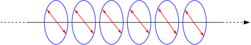
(a) Nematic state

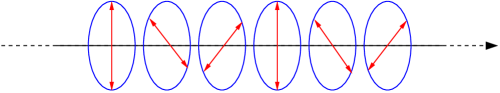
(b) $1/3$ state

Figure 3: Ground states structures for the chiral nematic clock system. (a) Nematic ordering for $0\leq\Psi<1/2$. (b) Chiral, right-handed, ordering with wavenumber $q=2\pi/3$ for $1/2<\Psi\leq 1$.

It is easy to analyze a number of statistical properties of one-dimensional models with chiral short-range bonds. For the particular system we are investigating, with ramification $r=1$, it is possible to show that

$$\left(\begin{array}[c]{c}Z_{1}^{\prime}\\ Z_{2}^{\prime}\\ Z_{3}^{\prime}\end{array}\right)=\mathbf{M}\,\left(\begin{array}[c]{c}Z_{1}\\ Z_{2}\\ Z_{3}\end{array}\right),$$ (24)

where $\mathbf{M}$ is a cyclic matrix,

$$\mathbf{M}\,=\left(\begin{array}[c]{ccc}A&B&C\\ C&A&B\\ B&C&A\end{array}\right).$$ (25)

The eigenvalues of this cyclic matrix are given by

$$\begin{split}\Lambda_{0}&=A+B+C,\\ \Lambda_{\pm}&=A-\frac{1}{2}\left(B+C\right)\pm i\frac{\sqrt{3}}{2}\left(B-C\right).\end{split}$$ (26)

Note the presence of the complex conjugate eigenvalues $\Lambda_{+}$ and $\Lambda_{-}$, which lead to an oscillating decay of the pair correlation function for most values of $\Delta$. This is already an indication of the existence of spatially modulated structures in larger dimensional systems. The fixed point, $\rho_{1}^{\ast}=\rho_{2}^{\ast}=1/3$, is linearly stable, except at zero temperature. In addition to the complex structure of correlations for non-zero temperatures, the model also presents a rich ground state physics, which is more appropriated to investigate by means of a dimensionless chiral field,

$$\Psi=\frac{3\Delta}{\pi}.$$ (27)

As a result, one can notice that the ground state behavior is the nematic analogous of the ferromagnetic CC Hamiltonians[31, 7]. Then, for $0\leq\Psi<1/2$, the ground state is of nematic type, where all nematic clocks are in the same orientational state, as indicated schematically in Figure 3a. However, for $1/2<\Psi\leq 1$, the system exhibits a right-handed helical ordering, with modulation $q=2\pi/3$ (period $3$), along the chiral direction (see Figure 3b ). The special chiral field value $\Psi=1/2$ leads the system to an infinitely degenerated ground state, with finite zero-temperature entropy, usually called multiphase point [6, 7]. We expect, as discussed in the context of ANNNI models [6] and CC spin systems [31], that thermal fluctuations may break the ground state degenerescence, which can give rise to nontrivial phase behavior for finite temperatures.

4 Mean-field limit and phase behavior

We now resort to a well known technique to obtain mean-field results from the recursion relations on a Cayley tree. We take an “infinite coordination limit”, $r\to\infty$ and $J\to 0$, while keeping the product $rJ$ fixed. In this limit, the nonlinear map becomes somewhat more feasible to deal with, which allows us to grasp the main qualitative features of this problem.

In the infinite coordination limit, equations (19) can be rewritten as

$$\rho_{1}^{\prime}=\frac{\exp\left(\beta JrM_{1}\right)}{{\displaystyle\sum\limits_{i=1}^{3}}\exp\left(\beta JrM_{i}\right)},\quad\rho_{2}^{\prime}=\frac{\exp\left(\beta JrM_{2}\right)}{{\displaystyle\sum\limits_{i=1}^{3}}\exp\left(\beta JrM_{i}\right)},$$ (28)

with

$$\begin{split}M_{1}&=-\frac{1}{4}\left(\cos 2\Delta+\sqrt{3}\sin 2\Delta\right)+\frac{1}{4}\left(3\cos 2\Delta+\sqrt{3}\sin 2\Delta\right)\rho_{1}+\\ &\qquad+\frac{\sqrt{3}}{2}\left(\sin 2\Delta\right)\rho_{2},\\ &\\ M_{2}&=-\frac{1}{4}\left(\cos 2\Delta-\sqrt{3}\sin 2\Delta\right)-\frac{\sqrt{3}}{2}\left(\sin 2\Delta\right)\rho_{1}+\\ &\qquad+\frac{1}{4}\left(3\cos 2\Delta-\sqrt{3}\sin 2\Delta\right)\rho_{2},\\ &\\ M_{3}&=\frac{1}{2}\cos 2\Delta-\frac{1}{4}\left(3\cos 2\Delta-\sqrt{3}\sin 2\Delta\right)\rho_{1}-\\ &\qquad-\frac{1}{4}\left(3\cos 2\Delta+\sqrt{3}\sin 2\Delta\right)\rho_{2}.\end{split}$$ (29)

The system of coupled nonlinear equations (28) can be solved iteratively, and the solutions allow us to draw the global phase diagram as well the behavior of the modulation as a function of model parameters.

It is immediate to show that the mean-field equations (28) lead to a disordered fixed point,

$$\rho_{1}^{\ast}=\rho_{2}^{\ast}=\frac{1}{3},$$ (30)

for all values of temperature and chiral parameter. A linear analysis of stability indicates that this disordered solution is unstable below a certain limiting reduced temperature,

$$T\equiv\frac{1}{\beta rJ}=\frac{1}{4},$$ (31)

for all values of $\Delta$. The eigenvalues of the recursion relations (28) about this trivial fixed point are a pair of complex conjugates,

$$\lambda_{\pm}=\frac{\beta Jr}{4}\left(\cos 2\Delta\pm i\sin 2\Delta\right),$$ (32)

which is an indication of the transition to a modulated structure.

In particular, for the case $\Delta=0$, which corresponds to absence of chirality, recursion relations (28) are reduced to simple expressions,

$$\begin{split}\rho_{1}^{\prime}&=\frac{\exp\left(c\rho_{1}\right)}{\exp\left(c\rho_{1}\right)+\exp\left(c\rho_{2}\right)+\exp\left[c\left(1-\rho_{1}-\rho_{2}\right)\right]},\\ &\\ \rho_{2}^{\prime}&=\frac{\exp\left(c\rho_{2}\right)}{\exp\left(c\rho_{1}\right)+\exp\left(c\rho_{2}\right)+\exp\left[c\left(1-\rho_{1}-\rho_{2}\right)\right]},\end{split}$$ (33)

where $c=3\beta Jr/4$. As a result, one can check that the disordered fixed point, $\rho_{1}^{\ast}=\rho_{2}^{\ast}=1/3$, is stable at high temperatures, $\beta Jr<4$. There is also an ordered fixed point, $\rho_{1}^{\ast}=\rho_{2}^{\ast}=\rho^{\ast}\neq 1/3$, which comes from the equation

$$\frac{9}{4}\beta Jrw=\ln\frac{1+6w}{1-3w},$$ (34)

where

$$\rho^{\ast}=\frac{1}{3}-w,$$ (35)

which is the standard mean-field equation for the three-state Potts model. However, it is important to mention that there is always a disordered solution, $w=0$. At low temperatures, for $\beta Jr<4$, it is also possible to notice that there is another (ordered) solution, $w\neq 0$. However, a careful numerical analysis of (34) shows that the ordered solution is already present in a small range of temperatures $T>1/4$, which is a typicalfeature of first-order transitions.

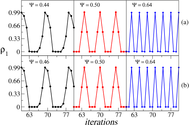
Figure 4: Examples of the behavior of $\rho_{1}$ in periodic solutions (the behavior of $\rho_{2}$ is identical up to a horizontal shift) for (a) $T=0.05$ and (b) $T=0.03$. The values of dimensionless chiral field $\Psi$ and reduced temperature $T$ have been chosen to obtain short periods.

In order to study the phase behavior of the model, we perform extensive numerical investigations of the MF equations (28), which we may write as

$$\begin{split}\rho_{1}^{\prime}&=f_{1}\left(\rho_{1},\rho_{2}\right),\\ \rho_{2}^{\prime}&=f_{2}\left(\rho_{1},\rho_{2}\right),\end{split}$$ (36)

Such set of coupled nonlinear equations can be solved by means of iterative procedures. It is worth to mention that due to the Cayley tree structure, MF equations express a relation between densities $\rho_{1}$ and $\rho_{2}$ along the generations. In practice, we have a nonlinear mapping problem, where primed densities $\rho_{1}^{\prime}$ and $\rho_{2}^{\prime}$, associated with some generation, which we call $s$, are related to unprimed densities $\rho_{1}$ and $\rho_{2}$ of generation $s-1$. Then, for fixed $T$ and $\Psi$ given by (27), we start with different initial conditions and let iterate the map (36) until it reaches some kind of stationary behavior whose features determine the character of the nature of the phase. As for usual maps, e.g. those describing dynamical systems (see e.g. [32]), we find many different types of solutions, specifically fixed points and periodic orbits.

As it is sketched above, for $\Psi=0$ there is a disordered, or isotropic, phase $\rho_{1}=\rho_{2}=1/3$. We shall see below that this phase appears at sufficiently high temperature, even for $\Psi\neq 0$. Similarly, stationary fixed points with different densities, $\rho_{1}\neq 1/3$ and $\rho_{2}\neq 1/3$, characterize uniform nematic states and are found for values of $\Psi$ and $T$ in certain intervals. A different kind of stationary behavior is represented by periodic solutions, which appear for some range of parameters. In this case, $\rho_{1}$ and $\rho_{2}$ do not attain stationary values but change periodically. This corresponds to situations in which, instead of reaching a simple fixed point, $\left(\rho_{1}^{\ast},\rho_{2}^{\ast}\right)$, the map (36) flows to a more complex attractor. If the $n$th iterate of the map flows to a fixed point, $f_{i}^{\left(n\right)}=f_{i}\left(f_{i}\left(...f_{i}\left(\rho_{1},\rho_{2}\right)\right)\right)$, we have a solution of period $n$, as it is shown in Figure 4. periods can be obtained by varying the dimensionless chiral field $\Psi$ and the reduced temperature $T$. These solutions can be interpreted as modulated phases, in which the typical angle changes along the tree from one generation to the next, giving room to genuine chiral phases.

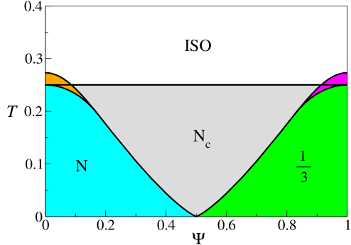
Figure 5: Phase diagram of the chiral nematic clock model with restricted orientations; $T$ is the reduced temperature and $\Psi$ is the dimensionless chiral field. We indicate an isotropic phase (ISO), a nematic phase (N_c), and a modulated nematic phase with wave number $q=2\pi/3$, which we call $1/3$. Region N_c is occupied by a multitude of chiral nematic phases. Orange and magenta regions present distinct attractors associated with nearby phases.

The main features of the global phase diagram of the model are sketched in Figure 5, where $T$ is the reduced temperature and $\Psi$ is the dimensionless chiral field given by (27). It is important to bear in mind that we have a lattice model on a Cayley tree, which means that phase boundaries are in fact the stability limit of phases. Also, due to symmetry properties of the model (11), the phase boundaries are symmetrical with respect to the dimensionless chiral field $\Psi=1/2$. In fact, we only need to study the system for $0\leq\Psi\leq 1/2$ and map the MF results into $1/2\leq\Psi\leq 1$ through (11) and (27). We can identify the region of stability of the nematic phase, which is favoured for $0\leq\Psi<1/2$ and sufficient low as well intermediate temperatures. Otherwise, a nematic chiral structure, with modulation $q=2\pi/3$, is stable for $1/2\leq\Psi<1$, but its stability region tends to shrink as temperature increases. Nevertheless, for chiral fields in the vicinity of the multiphase point, $\Psi=1/2$, thermal fluctuations lead to a fan-shaped region, with many different stable chiral structures (N_c), between N and $1/3$ states. As expected, the isotropic phase (ISO) is stable for temperatures $T>1/4$.

The CNC model is an effectively discrete-state spin system closely related to the Potts model. The well known mean-field results for the $3$-state Potts model describe a discontinuous transition between disordered and ordered phases [28]. However, for many discrete statistical models defined on Cayley trees, it is very complicated to properly characterize the type of transition, even by taking the infinite coordination limit, which corresponds to mean-field theory. In spite of the difficulties to deal with specific aspects of transitions, our numerical investigations show regions which present distinct types of attractors. These overlapping regions are indications of phase coexistence as well metastability, which are associated with first-order phase transitions. In Figure 5, the orange region is occupied by N and ISO states, for temperatures $T>1/4$, but presents attractors consistent with N and N_c, for $T<1/4$. Otherwise, in the magenta region, we find N and $1/3$ solutions for $T>1/4$, but it is occupied by $1/3$ and N_c for temperatures $T<1/4$.

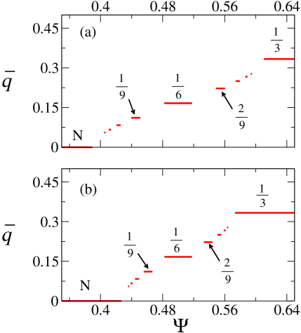
Figure 6: Dimensionless wavenumber $\overline{q}$ as a function of the dimensionless chiral field $\Psi$ for reduced temperatures (a) $T=0.05$ and (b) $T=0.03$. Modulation locks-in some commensurate, nematic-like, chiral phases. Cholesteric pitch exhibits a staircase behavior.

The green region occupied by chiral phases is strongly influenced by thermal fluctuations. As a result, the modulation presents a nontrivial behavior as a function of temperature and chiral field. Figure 6 shows the dimensionless wavenumber $\overline{q}=q/2\pi$ as a function of chiral field $\Psi$ for different values of temperature. Notice that, at low-temperature regimes, the modulation locks-in at some rational values of the type $\overline{q}=L/M$, such as the densities $\rho_{1}$ and $\rho_{2}$, which are related to the order parameter, evolves along the generations performing a periodic structure with $L$ turns in $M$ iterations. Although we only show phases with small values of $M$, we emphasize that long-periodic modulated structures are also presented, specially as $T$ increases. In general, one can notice that, for a given temperature, as the chiral field increases, N melts into the modulated region, which presents a multitude of modulated phases, and a sequence of transitions are observed, until the $1/3$ state is reached. It is possible to show a similar behavior (emergence of successive chiral structures) if one considers variations of $T$ for constant $\Psi$ values. Note that we only indicate some commensurate phases, but incommensurate states may be found at intermediate temperatures, as well as a nontrivial branching mechanism associated with the regions occupied by chiral, nematic-like, phases with different modulations [6].

An analogous staircase-like behavior is presented in the ANNNI and CC models. However, even more sophisticated phase sequences are also observed, where the modulation, as a function of model parameters, exhibits a fractal structure, which is called devil’s staircase [29, 30, 8]. Therefore, we argue that the nematic clock model with chiral interactions exhibits nematic chiral phases with temperature-dependent pitch. In fact, we do believe the CNC model may also present a case of devil’s staircase modulation behavior. These peculiar staircases are characterized by a Hausdorff dimension which depends on temperature. For the CNC system, it should be interesting, as a further investigation, the study of the fractal character associated with the cholesteric pitch.

5 Conclusions

We have shown that the Lebwohl-Lasher model used to describe the nematic-isotropic transition in liquid crystals, with the restriction of the microscopic nematic directors to point along $p$ planar directions, gives rise to a nematic counterpart of a $p$-state clock model. We then introduced chiral interactions between first-neighbor sites along a lattice direction, according to a mechanism of chirality that has been used to explain different forms of helimagnetism. The resulting $XY$ chiral Lebwohl-Lasher statistical model, which we call CNC model, is the nematic counterpart of the well-investigated (magnetic) chiral clock models.

On the basis of previous calculations for the analogous magnetic models, we formulated the statistical problem as a non linear map along the branches of a Cayley tree. It is known that attractors of this map correspond to solutions of physical interest. Also, in a suitable limit of infinite coordination of the tree, equations are somewhat simplified, and we are supposed to recover standard mean-field results. We take full advantage of the Cayley tree to investigate the presence of stable modulated structures.

In this preliminary work, we performed some explicit calculations for a restricted-orientation chiral clock model with head-tail symmetry. Besides the isotropic and nematic phases, we have shown the existence of sequences of modulated structures, with a pitch that depends on temperature and a parameter of chirality. A global phase diagram is presented, where it is possible to identify uniform ordered states as well spatially modulated phases. These sketchy calculations, however, are sufficient to illustrate the origins and the main qualitative features of modulation associated with helical nematics (cholesteric states) in liquid-crystalline systems. We hope this investigation will be a guide for future (and more extensive)work, including connections with earlier calculations for statistical molecular models [22, 21, 23] and predictions of the phenomenological elastic theories [18].

Appendix A $4$-state nematic chiral clock model

We now use a similar approach to analyze a four-state $XY$ chiral Lebwohl-Lasher model. We consider just two traceless tensor microscopic states,

$$\mathbf{Q}\left(1\right)=\frac{1}{2}\left(\begin{array}[c]{cc}1&0\\ 0&-1\end{array}\right),\quad\mathbf{Q}\left(2\right)=\frac{1}{2}\left(\begin{array}[c]{cc}-1&0\\ 0&1\end{array}\right),$$ (37)

from which we write the recursion relations

$$\begin{split}Z_{1}^{\prime}&=\left[Z_{1}\exp\left(\frac{1}{2}\beta J\cos 2\Delta\right)+Z_{2}\exp\left(-\frac{1}{2}\beta J\cos 2\Delta\right)\right]^{r}\\ Z_{2}^{\prime}&=\left[Z_{1}\exp\left(-\frac{1}{2}\beta J\cos 2\Delta\right)+Z_{2}\exp\left(\frac{1}{2}\beta J\cos 2\Delta\right)\right]^{r}.\end{split}$$ (38)

We then introduce the density variables

$$\rho_{i}=\frac{Z_{i}}{Z_{1}+Z_{2}},$$ (39)

for $i=1,2$, so that the problem is reduced to a one-dimensional map,

$$\rho_{1}^{\prime}=\frac{1}{D_{4}}\left[\exp\left(-\frac{1}{2}\beta J\cos 2\Delta\right)+2\rho_{1}\sinh\left(\frac{1}{2}\beta J\cos 2\Delta\right)\right]^{r},$$ (40)

with

$$D_{4}=\left[\exp\left(-\frac{1}{2}\beta J\cos 2\Delta\right)+2\rho_{1}\sinh\left(\frac{1}{2}\beta J\cos 2\Delta\right)\right]^{r}+$$ (41)

$$+\left[\exp\left(\frac{1}{2}\beta J\cos 2\Delta\right)-2\rho_{1}\sinh\left(\frac{1}{2}\beta J\cos 2\Delta\right)\right]^{r}.$$

Taking into account that

$$Q=\left\langle Q_{11}\right\rangle=\frac{1}{2}\rho_{1}-\frac{1}{2}\rho_{2}=\rho_{1}-\frac{1}{2},$$ (42)

this map can be written as $Q^{\prime}=f\left(Q\right)$.

In the limit of infinite coordination ($r\rightarrow\infty$, $J\rightarrow 0$, with fixed values of $rJ$), we have the simple form

$$Q^{\prime}=\frac{1}{2}\tanh\left[\beta Jr\cos\left(2\Delta\right)Q\right],$$ (43)

from which we see that the disordered fixed point is linearly stable for

$$\frac{k_{B}T}{rJ}>\left|\frac{1}{2}\cos 2\Delta\right|.$$ (44)

In the $T-\Delta$ phase diagram, besides a trivial ferromagnetic structures, there is only a quite trivial antiferromagnetic arrangement.

References

- [1] M. Seul and D. Andelman, Science, 267, 476–483 (1995).
- [2] D. Andelman and R. E. Rosensweig, J. Phys. Chem. B 113, 3785–3798 (2009).
- [3] A. Giuliani, Joel L. Lebowitz and Elliott H. Lieb, AIP Conference Proceedings 1091, 44-54 (2009).
- [4] W. Selke, “Spatially modulated structures in systems with competing interactions” in Phase Transitions and Critical Phenomena, Vol. 15, p.1-72, ed. by C. Domb and J.L. Lebowitz (Academic Press, 1992).
- [5] P. Bak, Repts. Progr. Phys. 45, 587 (1982).
- [6] W. Selke, Phys. Rep. 170, 213 (1988).
- [7] J. Yeomans, Sol. State Phys. 41, 151 (1988).
- [8] E. S. Nascimento, J. P. de Lima and S. R. Salinas, Physica A 409, 78–86 (2014).
- [9] Yu. A. Izyumov, Sov. Phys. Usp. 27, 845 (1984).
- [10] J. Kishine, K. Inoue, Y. Yoshida, Progr. Theor. Phys. Suppl. 159, 82 (2005).
- [11] M. Shinozaki, S. Hoshino, Y. Masaki, J. Kishine, Y. Kato, J. Phys. Soc. Jpn. 85, 074710 (2016); T. Toretsume, T. Kikuchi, R. Anita, J. Phys. Soc. Jpn. 87, 041011 (2018).
- [12] D. A. Huse, Phys. Rev. B 24, 5180 (1981).
- [13] S. Ostlund, Phys. Rev. B 24, 398 (1981).
- [14] H. C. Öttinger, J. Phys. C 16, L257 (1983); J. Phys. C 16, L597 (1983).
- [15] M. Siegert and H. U. Everts, Z. Phys. B 60, 265 (1985).
- [16] M. Pleimling, B. Neubart, R. Siems, J. Phys. A 31, 4871 (1998).
- [17] P. G. de Gennes and J. Prost, The Physics of Liquid Crystals (Clarendon Press, Oxford, 1993).
- [18] R. D. Kamien and J. V. Selinger, J. Phys.: Condens. Matter 13, R1 (2001).
- [19] J. V. Selinger, Introduction to the Theory of Soft Matter: From Ideal Gases to Liquid Crystals (Springer, New York, 2016).
- [20] W. J. A. Goossens, Mol. Cryst. Liq Cryst. 12, 237-244 (1971).
- [21] B. W. van der Meer, G. Vertogen, A. J. Dekker and J. G. J. Ypma, J. Chem. Phys. 65, 3935 (1976).
- [22] B. C. H. Krutzen and G. Vertogen, Liq. Cryst. 6, 211 (1989).
- [23] Y. R. Lin-Liu, Yu Ming Shih, Chia-Wei Woo, and H. T. Tan, Phys. Rev. A 14, 445 (1975)
- [24] P. A. Lebwohl and G. Lasher, Phys. Rev. A 6, 426 (1972).
- [25] S R. Salinas and E. S. Nascimento, Mol. Cryst. Liq. Cryst. 657, 27 (2017).
- [26] C. S. O. Yokoi and M. J. de Oliveira, J. Phys. A 18, L153 (1985); A. T. Bernardes and M. J. de Oliveira, J. Phys. A 25, 1405 (1992).
- [27] M. J. de Oliveira and S. R. Salinas, J. Phys. A 18, L1157 (1985); C. S. O. Yokoi, M. J. de Oliveira, and S. R. Salinas, Phys. Rev. Lett. 54, 163 (1985).
- [28] F. Y. Wu, Rev. Mod. Phys. 54, 235 (1982).
- [29] P. Bak, Physics Today 39, 38 (1986).
- [30] W. Selke and P. Bak, Physics Today 40, 116 (1987).
- [31] J. Yeomans, J. Phys. C: Solid State Phys. 15, 7305 (1982).
- [32] M. Cencini, F. Cecconi and A.Vulpiani CHAOS: From Simple Models to Complex Systems (World Scientific, Singapore 2009).