Robot Localization in Floor Plans
Using a Room Layout Edge Extraction Network

Abstract

Indoor localization is one of the crucial enablers for deployment of service robots. Although several successful techniques for indoor localization have been proposed, the majority of them relies on maps generated from data gathered with the same sensor modality used for localization. Typically, tedious labor by experts is needed to acquire this data, thus limiting the readiness of the system as well as its ease of installation for inexperienced operators. In this paper, we propose a memory and computationally efficient monocular camera-based localization system that allows a robot to estimate its pose given an architectural floor plan. Our method employs a convolutional neural network to predict room layout edges from a single camera image and estimates the robot pose using a particle filter that matches the extracted edges to the given floor plan. We evaluate our localization system using multiple real-world experiments and demonstrate that it has the robustness and accuracy required for reliable indoor navigation.

I Introduction

Inexpensive sensors and ease of setup are widely considered as key enablers for a broad diffusion of consumer-grade robotic applications. However, such requirements pose technological challenges to manufacturers and developers due to the limited quantity of sensory data and low quality of prior information available to the robot. Particularly in the context of robot navigation, most of the existing localization solutions require highly accurate maps that are built upfront with the same sensor modality used for localizing the robot. Typically, these maps are generated by collecting sensory measurements via teleoperation and fusing them into a coherent representation of the environment using Simultaneous Localization and Mapping (SLAM) algorithms. Despite the advances in the field, maps generated by SLAM systems can be affected by global inconsistencies when perceptual aliasing or feature scarcity reduce the effectiveness of loop closing approaches. In general, substantial expertise is required to assess whether the quality of the generated maps is sufficient for the planned deployment. For large-scale environments such as office buildings, teleoperating the platform through the entire navigable area can be a tedious and time-consuming operation. In order to address these issues, previous works [1, 2, 3] have proposed to leverage floor plans obtained from architectural drawings for accurate localization as they provide a representation of the stable structures in the environment. Furthermore, floor plans are often available from the blueprints used for the construction of buildings. Alternatively, floor plans can also be created with moderate effort using drawing utilities.

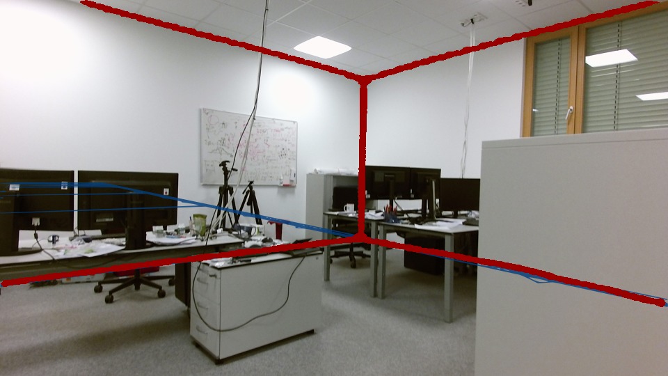
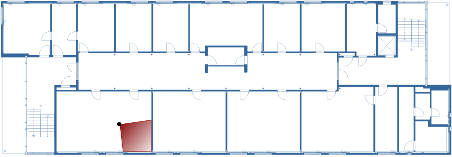
Figure 1: Our approach uses the proposed network to extract the room layout edges from an image (top) and compares it to a layout generated from a floor plan (bottom) to localize the robot. Our network is able to accurately predict layout edges even under severe occlusion, enabling robust robot localization.

Recently, computationally efficient approaches based on Convolutional Neural Networks (CNNs) have been proposed for extracting structural information from monocular images. This includes methods to extract room layout edges from images [4, 5]. However, these networks occasionally predict discontinuous layout edges, even more in the presence of significant clutter. In addition, room layouts can be inferred from floor plans under the assumption that buildings consist only of orthogonal walls, also called Manhattan world assumption [6], and have constant ceiling height.

Inspired by these factors, we propose a localization system that uses a monocular camera and wheel odometry to estimate the robot pose using a given floor plan. We propose a state-of-the-art CNN architecture to predict room layout edges from a monocular image and apply a Monte Carlo Localization (MCL) method that compares these edges with those inferred from a given floor plan. We evaluate our proposed method in real-world scenarios, showing its robustness and accuracy in challenging environments.

II Related Work

Several methods have been proposed to localize robots or, more generally, devices, in 2D maps using RGB and range/depth measurements. For example, the approaches proposed by Wolf et al. [7] and Bennewitz et al. [8] use MCL and employ a database of images recorded in an indoor environment. Mendez et al. [9] proposed a sensor model for MCL that leverages the semantics of the environment, namely doors, walls and windows, obtained by processing RGB images with a CNN. They enhance the standard likelihood fields for the occupied space on the map with suitable likelihood fields for doors and windows. Although such a sensor model can be also adapted to handle range-less measurements, it shows increased accuracy with respect to standard MCL only when depth measurements are used. Winteralter et al. [2] proposed a sensor model for MCL to localize a Tango tablet in a floor plan. They extrude a full 3D model from the floor plan and use depth measurements to estimate the current pose. More recently, Lin et al. [10] proposed a joint estimation of the camera pose and the room layout using prior information from floor plans. Given a set of partial views, they combine a floor plan extraction method with a pose refinement process to estimate the camera poses.

The approaches described above rely on depth information or previously acquired poses. Other methods only use monocular cameras to localize. Zhang and Kogadoga [11] proposed a robot localization system based on wheel odometry and monocular images. The system extracts edges from the image frame and converts the floor edges into 2D world coordinates using the extrinsic parameters of the camera. Such points are then used as virtual endpoints for vanilla MCL. A similar approach by Unicomb et al. [12] was proposed recently to localize a camera in a 2D map. The authors employ a CNN for floor segmentation from which they identify which lines in an edge image belong to the floor plan. The detected edges are reprojected into the 3D world using the current estimate of the floor plane. They are then used as virtual measurement in an extended Kalman filter. Hile and Boriello [13] proposed a system to localize a mobile phone camera with respect to a floor plan by triangulating suitable features. They employ RANSAC to estimate the relative 3D pose together with the feature correspondences. Although the system achieves high accuracy, the features are limited to corner points at the base of door frames and wall intersections. Therefore, the system is not usable outside corridors, due to occlusions and the limited camera field-of-view. Chu et al. [14] use MCL to estimate the 3D pose of a camera in an extruded floor plan. They proposed a sensor model that incorporates information about the observed free-space, doors as well as structural lines of the environment by leveraging a 3D metrical point cloud obtained from monocular visual SLAM.

The method proposed in this work differs from the approaches above. Instead of locally reconstructing the 3D world from camera observations and matching this reconstruction to an extruded model of the floor plan, we project the lines extracted from the floor plan into the camera frame. Our approach shares similarity with the work of Chu and Chen [15], Wang et al. [16] and Unicomb et al. [12]. In the first two works the authors localize a camera using a 3D model extracted from a floor plan. In order to score localization hypotheses, both systems use a distance-transform-based cost function that encodes the misalignment on the image plane between the structural lines extracted from the 3D model and the edge image obtained by edge detection. In contrast to these approaches, we use a CNN to reliably predict room layout edges in order to better cope with occlusion due to clutter and furniture. Unicomb et al. [12] also employ a CNN but they only learn to extract floor edges which is a limitation in the case of clutter or occlusions. Furthermore, using a Kalman Filter approach to project the measurement into the floor plan of the map can make the system less robust to wrong initialization as the accuracy of the virtual measurement is dependent on the current camera pose estimation. Finally, in contrast to [14] and [16], we model the layout edges of the floor plan from an image and wall corners without any prior 3D model.

Most of the CNN-based approaches for estimating room layout edges employ a encoder-decoder topology with a standard classification network for the encoder and utilize a series of deconvolutional layers for upsampling the feature maps [4, 5, 17, 12]. Ren et al. [17] proposed an architecture that employs the VGG-16 network for the encoder followed by fully-connected layers and deconvolutional layers that upsample to one quarter of the input resolution. The use of fully-connected layers enables their network to have a large receptive field but at the cost of loosing the feature localization ability. Lin et al.  [4] introduced a similar approach with the stronger ResNet-101 backbone and model the network in a fully-convolutional manner. Most recently, Zhang et al. [5] proposed an architecture based on the VGG-16 backbone for simultaneously estimating the layout edges as well as predicting the semantic segmentation of the walls, floor and ceiling. In contrast to these networks, we employ a more parameter efficient encoder with dilated convolutions and incorporate the novel eASPP [18] for capturing large context, complemented with an iterative training strategy that enables our network to predict thin layout edges without discontinuities.

III Proposed Method

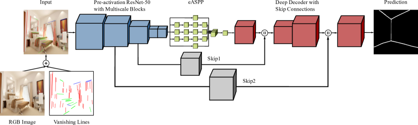
Figure 2: Topology of our proposed architecture for extracting room layout edges that builds upon our AdapNet++ model [18]. The network takes colorized vanishing lines overlaid on the monocular image as input and reliably predicts the room layout edges.

In order to localize the robot in floor plans, we employ MCL [19] with adaptive sampling. MCL applies Bayesian recursive update

$$bel(\mathbf{x}_{t})$$ (1)

$$\propto p(\mathbf{z}_{t}\mid\mathbf{x}_{t})\int_{X}p(\mathbf{x}_{t}\mid\mathbf{x}_{t-1},\mathbf{u}_{t})bel(\mathbf{x}_{t-1})d\mathbf{x}_{t-1}$$

to a set of weighed hypothesis (particles) for the posterior distribution $bel(\mathbf{x}_{t})\triangleq p(\mathbf{x}_{t}\mid\mathbf{z}_{1:t},\mathbf{u}_{1:t})$ of the robot pose $\mathbf{x}_{t}\in\mathbb{SE}(2)$, given a sequence of motion priors $\mathbf{u}_{1:t}$ and sensor measurements $\mathbf{z}_{1:t}$. Whereas a natural choice for the proposal distribution $p(\mathbf{x}_{t}\mid\mathbf{x}_{t-1},\mathbf{u}_{t})$ is to apply the odometry motion model with Gaussian noise, a suitable measurement model $p(\mathbf{z}_{t}\mid\mathbf{x}_{t})$ based on the floor plan layout edges has to be used, which we outline in the reminder of this section. To resample the particle set, we use KLD-sampling, which is a well known sampling technique that adapts the number of particles according to the Kullback-Leibler divergence of the estimated belief and is an approximation of the true posterior distribution [20].

Note that in this work, we are only interested in the pose tracking problem, that is, at every time $t>0$ we estimate $bel(\mathbf{x}_{t}\mid\mathbf{x}_{0})$ given an initial coarse estimate $\mathbf{x}_{0}\in\mathbb{SE}(2)$ of the starting location of the robot. For real-world applications, solving the global localization problem often not required as users can usually provide an initial guess for the starting pose of the robot.

III-A Room Layout Edge Extraction Network

Our approach to estimate the room layout edges consists of two steps. In the first step, we estimate the vanishing lines in a monocular image of the scene using the approach of Hedau et al. [21]. Briefly, we detect vanishing lines by extracting line segments and estimating three mutually orthogonal vanishing directions. Subsequently, we color the detected line segments according to the vanishing point using a voting scheme. In the second step, we overlay the estimated colorized vanishing lines on the monocular image which is then input to our network for feature learning and prediction. Utilizing the vanishing lines enables us to encode prior knowledge about the orientation of the surfaces in the scene which accelerates the training of the network and improves the performance in highly cluttered scenes.

The topology of our proposed architecture for learning to predict room layout edges is shown in Figure 2. We build upon our recently introduced AdapNet++ architecture [18] which has four main components. It consists of an encoder based on the full pre-activation ResNet-50 architecture [22] in which the standard residual units are replaced with multiscale residual units [23] encompassing parallel atrous convolutions with different dilation rates. We add dropout on the last two residual units to prevent overfitting. The output of the encoder, which is 16-times downsampled with respect to the input image, is then fed into the eASPP module. The eASPP module has cascaded and parallel atrous convolutions to capture long-range contexts with very large effective receptive fields. Having large effective receptive fields is critical for estimating room layout edges as indoor scenes are often significantly cluttered and the network needs to be able to capture large contexts beyond the occluded regions. In order to illustrate this aspect, we compare the empirical receptive field at the end of the eASPP of our network and the receptive field at the end of the full pre-activation ResNet-50 architecture in Figure 3. As we observe the receptive field for the pixel annotated by the red dot, we see that the receptive field at the end of the ResNet-50 architecture is not able to capture context beyond the clutter that causes occlusion, whereas the larger receptive field of our network allows to accurately predict the room layout edges even in the presence of severe occlusion.

In order to upsample the output of the eASPP back to the input image resolution, we employ a decoder with three upsampling stages. Each stage employs a deconvolution layer that upsamples the feature maps by a factor of two, followed by two $3\times 3$ convolution layers. We also fuse high-resolution encoder features into the decoder to obtain smoother edges. We use the parameter configuration for all the layers in our network as defined in the AdapNet++ architecture [18], except for the last deconvolution layer in which we set the number of filter channels to one and add a sigmoid activation function to yield the room layout edges, which is thresholded to yield a binary edge mask. We detail the training protocol that we employ in Section IV-B.

III-B Floor Plan Layout Edge Extraction

As in our previous work [24], we assume the floor plan to be encoded as binary image $\mathcal{I}\in\{\textsc{o},\textsc{f}\}^{H\times W}$ with resolution $\sigma$, a reference frame $\mathscr{F}\in\mathbb{SE}(2)$ and a set of corner points $C\subset\mathbb{R}^{2}$ associated to some corner pixels and expressed with respect to that reference frame. Corners are extracted by preprocessing the map using standard corner detection algorithms and clustering the resulting corners according to the relative distances in order to remove duplicates. We embed the above structure in the 3D world and assume the above entities to be defined in 3D while using the same notation.

(a) ResNet-50
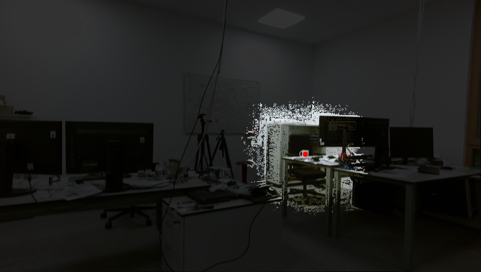
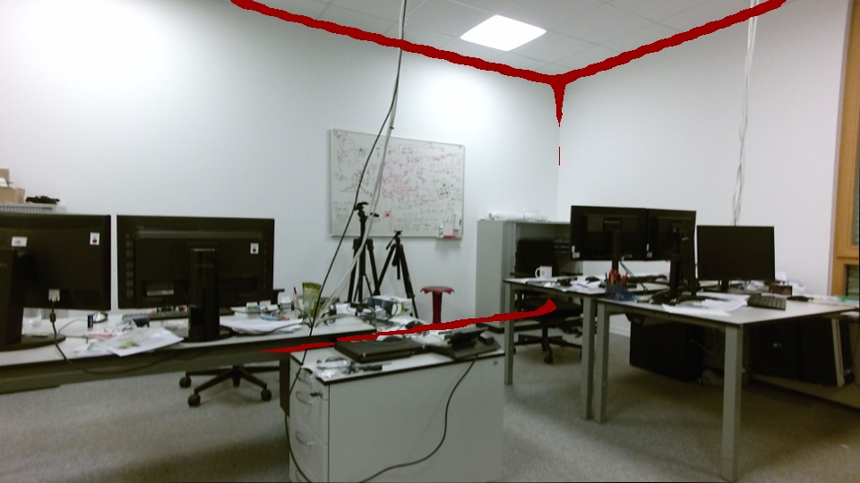
(b) Ours
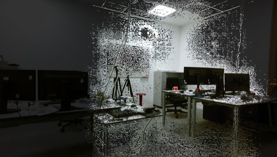
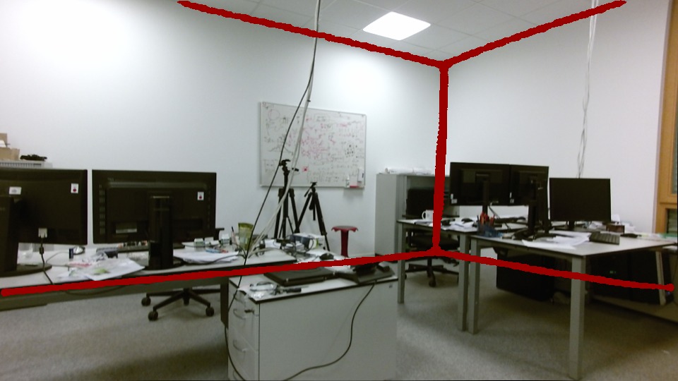
	Receptive Field	Prediction Overlay

Figure 3: Comparison of the receptive field at the end of the encoder for the pixel annotated by the red dot (left). Our network has a much larger effective receptive field than the standard ResNet-50 model, which enables us to capture large context. This results in a more exhaustive description of the room layout edges (right).

Similarly to Lin et al. [10], given a pose $\mathbf{x}\in\mathbb{SE}(3)$ on the floor plan and the extrinsic calibration parameters for the optical frame of the camera ${}^{\mathbf{r}}\mathbf{T}_{\mathbf{c}}\in\mathbb{SE}(3)$, we can estimate the orthogonal projection of the camera’s frustum onto the floor plan plane (see Figure 1). Observe that such projection defines two half-lines $\ell_{-}\triangleq\langle[\mathbf{x}\oplus{}^{\mathbf{r}}\mathbf{T}_{\mathbf{c}}]_{xy},\theta_{-}\rangle$ and $\ell_{+}\triangleq\langle[\mathbf{x}\oplus{}^{\mathbf{r}}\mathbf{T}_{\mathbf{c}}]_{xy},\theta_{+}\rangle$, where $[\mathbf{x}\oplus{}^{\mathbf{r}}\mathbf{T}_{\mathbf{c}}]_{xy}\in\mathbb{R}^{2}$ is the orthogonal projection of the origin of the optical frame onto the floor plan (origin of the half-lines), and $\theta_{\pm}\in(-\pi,\pi]$ are the ray directions with respect to the 2D reference frame $\mathscr{F}$. Such rays define an angular range $[\theta_{-},\theta_{+}]\subset(-\pi,\pi]$ that approximates the planar field-of-view (FoV) of the camera. Accordingly, we can approximate the layout room edges of the visible portion of the floor plan with a discrete set of points $O_{\mathbf{x}}\subset\mathbb{R}^{3}$ estimated or extruded from the floor plan image. More specifically, we construct $O_{\mathbf{x}}$ by inserting the points obtained by ray-casting within the camera FoV as well as their counterparts on the ceiling, obtained by elevating the ray-casted points by the height of the building, which we assume to be known upfront. Moreover, to complete the visible layout edges, we add to $O_{\mathbf{x}}$ those corners in $C$ whose lines of sight from $[\mathbf{x}\oplus{}^{\mathbf{r}}\mathbf{T}_{\mathbf{c}}]_{xy}$ fall within the 2D FoV of the camera together with their related ceiling points as well as the set of intermediate points sampled along the connecting vertical line (see Figure 4). The visibility of each corner point can be inferred, again, by ray-casting along the direction of each line of sight. Observe that, although ray-casting might be computationally expensive due to a high resolution $\sigma$, speed up can be achieved by ray-casting on floor plan images with a lower resolution.

III-C Measurement Model

Given an input image and the related layout edge mask $\mathbf{z}$, we define the observation model of each pose hypotheses as follows: for any pose $\mathbf{x}\in\mathbb{SE}(2)$ on the floor plan, we set

$$\log p(\mathbf{z}\mid\mathbf{x})=-\frac{1}{2|O_{\mathbf{x}}|\sigma_{z}^{2}}\sum_{o\in O_{\mathbf{x}}}\min\left\{d(\pi(o),\mathbf{z}),\delta\right\}^{2}$$ (2)

where $\delta>0$ (in pixel) is a saturation term used to avoid excessive down-weighing of particles whenever a measurement cannot be explained by the floor plan model, $\sigma_{z}>0$ (in pixel) is a tolerance term that encodes the expected pixel noise in the layout edge mask $\mathbf{z}$, $\pi(o)$ is the perspective camera transformation that projects 3D world points into the image plane, and $d(\mathrm{p},\mathbf{z})$ is the distance of pixel $\mathrm{p}$ to the closest pixel in edge layout mask.

Figure 4: Example of layout $O_{\mathbf{x}}$ extracted from the floor plan (blue) from a pose hypothesis $\mathbf{x}$. The floor points are obtained via ray-casting, the ceiling lines by projecting up the floor points and the wall edge is obtained from the corner point. The floorplan (light blue) is overlayed for illustration purposes. The measurement model compares $O_{\mathbf{x}}$ with the edge mask (red).

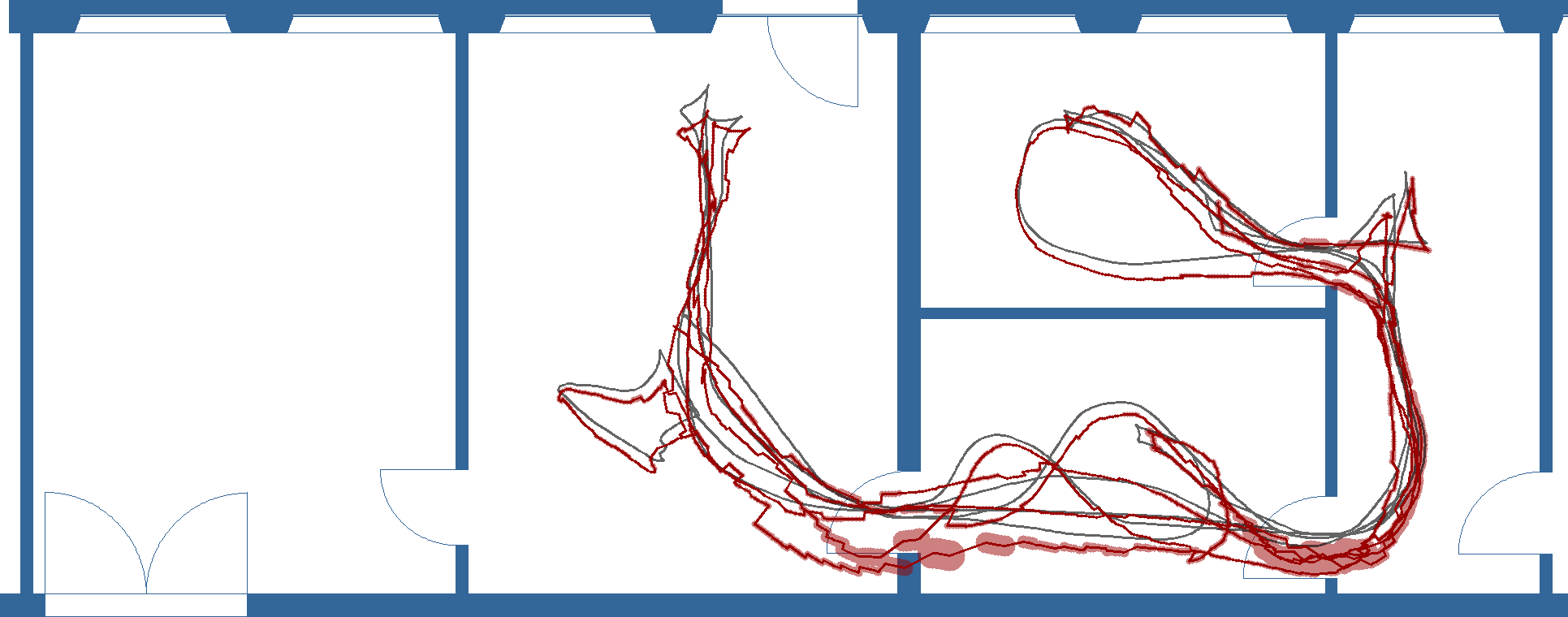
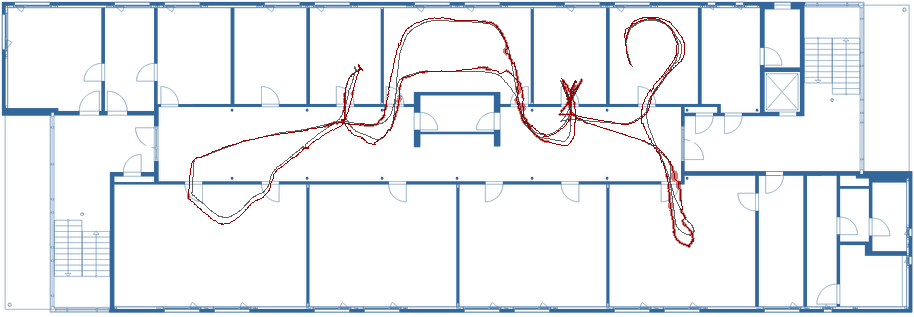
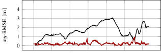
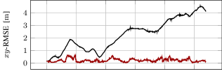
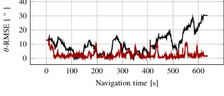
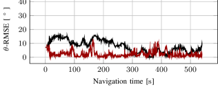
Figure 5: Accuracy of the localization system for Fr078-1 (left) and Fr080 (right). Top: the estimated mean trajectory (red) compared to the approximate ground-truth (gray). The red shadowed area represents the translational standard deviation of each pose estimate. Middle and bottom: The linear and angular RMSE (red) and the error produced by drifting odometry (black). The The red areas delimit the errors for the worst and best pose estimation.

IV Experimental Evaluation

To evaluate the performance of our proposed method, we recorded three datasets in two buildings of the University of Freiburg (building 078 and 080). We will henceforth refer to them as Fr078-1 ($113\text{\,}\mathrm{m}$ long), Fr078-2 ($179\text{\,}\mathrm{m}$ long) and Fr080 ($108\text{\,}\mathrm{m}$ long). Fr078-1 and Fr078-2 aim to emulate an apartment-like structure while Fr080 was obtained obtained in a standard office building. For all the experiments, we used a Festo Robotino omnidirectional platform and the RGB images obtained from a Microsoft Kinect V2 mounted on board the robot. The robot moved with an average speed of approximately $0.2\text{\,}\mathrm{m}\mathrm{/}\mathrm{s}$ and $15\text{\,}\mathrm{\SIUnitSymbolDegree}\mathrm{/}\mathrm{s}$ and maximum of $0.5\text{\,}\mathrm{m}\mathrm{/}\mathrm{s}$ and $50\text{\,}\mathrm{\SIUnitSymbolDegree}\mathrm{/}\mathrm{s}$. Since no ground-truth was available for these experiments, we employed the localization system proposed in [24] using an Hokuyo UTM-30LX laser rangefinder also mounted on the robot to provide a reference trajectory for the evaluation. Since the trajectories estimated by [24] are highly accurate, we will henceforth consider them to be the (approximate) ground-truth. For each dataset, we run $25$ experiments to account for the randomness of MCL and consider the estimated pose at each time to be the average pose over the runs.

In addition, we benchmark the performance of our room layout edge estimation network on the challenging LSUN Room Layout Estimation dataset [25] consisting of 4,000 images for training, 394 images for validation and 1,000 images for testing. We employ augmentation strategies such as horizontal flipping, cropping and color jittering to increase the number of training samples. We report results in terms of edge error, which can be computed as the Euclidean distance between the estimated layout edges and the ground-truth edge map, normalized by the number of pixel in each mask. In order to facilitate comparison with previous approaches [5], we also report the fixed contour threshold (ODS) and the per-image best threshold (OIS) [26] metrics.

IV-A Implementation

In all the experiments we used the same set of parameters. To extract the room layout of the floor plans we removed single pixel lines as well as close any doors gaps and narrow passages by using an erosion/dilation and dilation/erosion pass respectively on floor plans with resolution $\sigma=$1\text{\,}\mathrm{c}\mathrm{m}\mathrm{/}\textrm{px}$$. Similarly, the Harris corner detector implementation of OpenCV was utilized to extract the corner pixels on the floor plan image. In our implementation of MCL we set $\sigma_{z}=$10\text{\,}\textrm{px}$$ and $\delta=$25\text{\,}\textrm{px}$$. To compute the predicted layout $O_{\mathbf{x}}$, we subsampled the 2D camera FoV with $150$ rays and approximated the vertical edges of the layout with $100$ points. Localization updates occurred whenever the motion prior from wheel odometry reported a linear or angular relative motion exceeding $25\text{\,}\mathrm{cm}$ or approximately $15\text{\,}\mathrm{\SIUnitSymbolDegree}$ ($0.25\text{\,}\rad$) respectively and used 1,500 and 5,000 as minimum/maximum number of particles to approximate the robot belief.

IV-B Network Training

We used the TensorFlow deep learning library for the network implementation and we trained our model on images resized to a resolution of $320\times 320$ pixels. The output of our network has the same resolution as the input image. To generate the ground-truth data for training, we first converted the LSUN room layout ground-truth to a binary edge map where the edge lines have a width of 6 pixels. We dilated the edges with a $5\times 5$ kernel for $d_{e}$ number of iterations, where $e$ is the number of epochs for which we trained using this dilation factor. We then applied Gaussian blur with a kernel of $21\times 21$ pixels and $\sigma=6$ for smoothing the edge boundaries. We employed a four stage training procedure and began training with the ground-truth edges dilated with $d_{6}=5$ and in subsequent stages reduced the amount of edge dilation to $d_{14}=3$, $d_{20}=1$ and $d_{26}=0$. Intuitively this process can be described as starting the training with thick layout edges and gradually thinning the edge thickness as the training progresses. Employing this gradual thinning approach improves convergence and enables the network to predict precise thin edges, as opposed to training only with a fixed edge width. Lin et al. [4] employ a similar training strategy that adaptively changes the edge thickness according to the gradient, however our training strategy resulted in a better performance.

We used the He initialization [27] for all the layers of our network and the cross-entropy loss function for training. For optimization, we used Adam solver with $\beta_{1}=0.9$, $\beta_{2}=0.999$ and $\epsilon=10^{-10}$. Additionally, we suppressed the gradients of non-edge pixels by multiplying them with a factor of 0.2 in order to prevent the network from converging to zero, which often occurs due to the imbalance between edge and non-edge pixels. We trained our model for a total of 66 epochs with an initial learning rate of $\lambda_{0}=10^{-4}$ and a mini-batch size of 16, which takes about 18 hours on an NVIDIA TITAN X GPU.

IV-C Evaluation of Layout Edge Estimation

In order to empirically evaluate the performance of our room layout edge extraction network, we performed evaluations on the LSUN benchmark in comparison to state-of-the-art approaches [5, 4, 22]. The results are reported in Table I. Our network achieved an edge error of $8.33$ which corresponds to an improvement of $2.91$ over the previous state-of-the-art. We also observe higher ODS as well as OIS scores, thereby setting the new state-of-the-art on the LSUN benchmark for room layout edge estimation. The improvement achieved by our network can be attributed to its large effective receptive field, which enables it to capture more global context. Moreover, our iterative training strategy allows for estimation of thin layout edges without significant discontinuities.

Input Image	Lin et al. [4]	Zhang et al. [5]	Ours

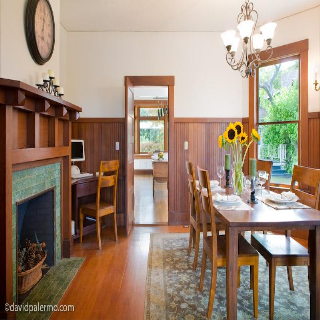
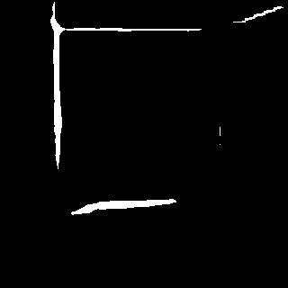
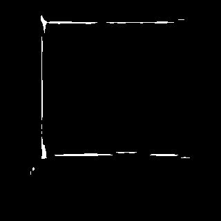
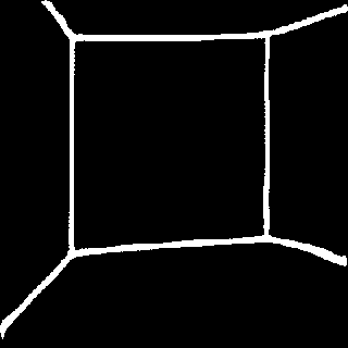
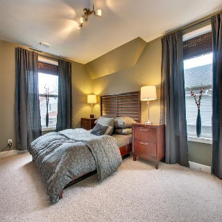
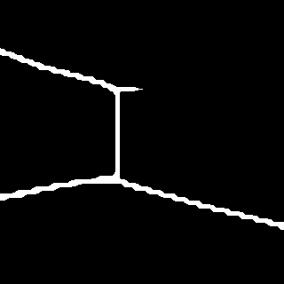
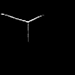
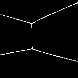
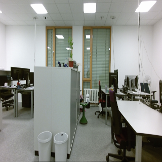
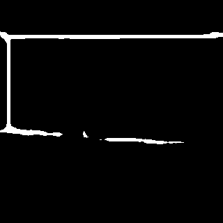
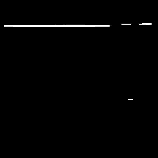
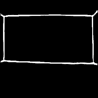
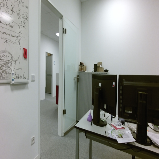
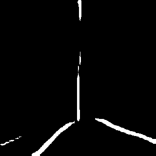
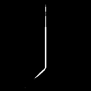
Figure 6: Qualitative room layout edge estimation results on the LSUN validation set (first two rows) and on Fr080 (last two rows). Compared to the other methods, our network reliably predicts continuous layout edges even under substantial occlusion.

Qualitative comparisons of room layout edge estimation are reported in Figure 6. The first two and last two rows show prediction results on the LSUN validation set and Fr080 dataset respectively. Note that we only trained our network on the LSUN training set. We can see that the previous state-of-the-art networks are less effective in predicting the layout edges in the presence of large objects in the scene that cause significant occlusions, whereas our network is able to leverage its large receptive field to more reliably capture the layout edges. We can also observe that the prediction of the other networks are more irregular and sometimes either too thin, thus resulting in discontinuous layouts, or too thick, reducing the effectiveness of the sensor model described in Section III-C. In these scenarios our network is able to accurately predict the layout edges without discontinuities and generalize effectively to previously unseen environments.

IV-D Ablation Study of Layout Edge Estimation Network

Table I: Benchmarking edge layout estimation on the LSUN dataset.

Network	Edge Error	ODS	OIS	Parameters
ResNet50-FCN [22]	18.36	0.213	0.227	23.57 M
Lin et al. [4]	10.72	0.279	0.284	42.29 M
Zhang et al. [5]	11.24	0.257	0.263	138.24 M
Ours	8.33	0.310	0.316	30.19 M

Table II: Layout edge estimation network configuration.

Model	Output	Background	Vanishing	Edge
	Resolution	Weight	Lines	Error
M1	1/4	0.0	-	10.99
M2	1/4	0.2	-	10.61
M3	1/2	0.2	-	10.13
M4	Full	0.2	-	9.46
M5	Full	0.2	✓	8.33

We evaluated the performance of our network through the different stages of the upsampling. Referring to Table II, the M1 model upsamples the eASPP output to one quarter the resolution of the input image and achieves an edge error of $10.99$. In the subsequent M2 and M3 models, we suppress the gradients of the non-edge pixels with a factor of 0.2 and upsample the eASPP output to half the resolution of the input image, which reduces the edge error by $0.86$. Finally, in the M4 model, we upsample back to the full input image resolution and in the M5 model we overlay the colorized vanishing lines by adding these channels to the RGB image. Our final M5 model achieves a reduction of $2.66$ in the edge error compared to base AdapNet++ model.

IV-E Localization Robustness and Accuracy

In all the experiments, the robot was initialized within $10\text{\,}\mathrm{cm}$ and $15\text{\,}\mathrm{\SIUnitSymbolDegree}$ from the ground-truth pose. As shown in Figure 5, the robot was always able to estimate its current pose and non negligible errors were reported only in a specific situation. As shown in Figure 5, in Fr078-1, the robot failed temporarily to track its current pose while traversing a doorway (scattered trajectory at the bottom of the map). The error was due to the camera image capturing both the next room (predominant view) and the current room (limited view). This caused the network to only predict the layout edges for largest room view, before having entered the next room. The linear RMSE of the mean trajectory reached approximately $1\text{\,}\mathrm{m}$. Nonetheless, the robot was subsequently able to localize itself with an accuracy similar to the average accuracy over the entire experiment whenever new observations were collected.

Overall, the proposed method delivered an average linear RMSE of $227\pm 137\text{\,}\mathrm{mm}$ and $245\pm 137\text{\,}\mathrm{mm}$ as well as an average angular RMSE of $2.5\pm 2.5\text{\,}\mathrm{\SIUnitSymbolDegree}$ and $2.5\pm 2.3\text{\,}\mathrm{\SIUnitSymbolDegree}$ in Fr078-1 and Fr078-2 respectively. Similar results were recorded for Fr080, with an average linear and angular RMSE of $223\pm 126\text{\,}\mathrm{mm}$ and $2.3\pm 2.0\text{\,}\mathrm{\SIUnitSymbolDegree}$ respectively.

IV-F Runtime

We used a 8-core $4.0\text{\,}\mathrm{GHz}$ Intel Core i7 CPU and a NVIDIA GeForce 980M GPU in all experiments. On average, the system required $30\pm 14\text{\,}\mathrm{ms}$ for the MCL update, while the inference time for the proposed network was $39\text{\,}\mathrm{ms}$. In addition, the Manhattan line extraction took $80\pm 116\text{\,}\mathrm{ms}$. The high peaks in Figure 7 are due to the Manhattan lines extraction step, which runs on an external Matlab script and therefore it can be further optimized. As shown in Figure 7, our proposed approach runs in real-time on consumer grade hardware.

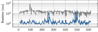
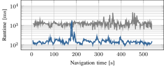
Figure 7: Total runtime in milliseconds (blue line) for the network processing and the localization update in Fr078-1 (top) and Fr080 (bottom). The gray line represents the available runtime between two consecutive localization updates. Each runtime is computed as average runtime over the runs.

V Conclusions

In this work, we presented a robot localization system that uses wheel odometry and images from a monocular camera to estimate the pose of a robot in a floor plan. We utilize a novel convolutional neural network tailored to predict the room layout edges and employ Monte Carlo Localization with a sensor model that scores the overlap of the predicted layout edge mask and the expected layout edges generated from a floor plan image. Experiments in complex real-world environments demonstrate that our proposed system is able to robustly estimate the pose of the robot even in challenging conditions such as severe occlusion. In addition, our network for room layout edge estimation achieves state-of-the-art performance on the challenging LSUN benchmark and generalize effectively to previously unseen environments with complex room layouts.

References

- [1] S. Ito, F. Endres, M. Kuderer, G. D. Tipaldi, C. Stachniss, and W. Burgard, “W-RGB-D: floor-plan-based indoor global localization using a depth camera and wifi,” in Proc. of the IEEE International Conference on Robotics and Automation, 2014.
- [2] W. Winterhalter, F. Fleckenstein, B. Steder, L. Spinello, and W. Burgard, “Accurate indoor localization for RGB-D smartphones and tablets given 2D floor plans,” in Proc. of the IEEE/RSJ International Conference on Intelligent Robots and Systems, 2015.
- [3] F. Boniardi, T. Caselitz, R. Kümmerle, and W. Burgard, “Robust LiDAR-based localization in architectural floor plans,” in Proc. of the IEEE/RSJ International Conference on Intelligent Robots and Systems, 2017.
- [4] H. J. Lin, S.-W. Huang, S.-H. Lai, and C.-K. Chiang, “Indoor scene layout estimation from a single image,” in Proc. of the IEEE International Conference on Pattern Recognition, 2018.
- [5] W. Zhang, W. Zhang, and J. Gu, “Edge-semantic learning strategy for layout estimation in indoor environment,” arXiv preprint arXiv:1901.00621, 2019.
- [6] J. Coughlan and A. Yuille, “Manhattan world: Orientation and outlier detection by Bayesian inference,” Neural Computation, vol. 15, no. 5, pp. 1063–1088, 2003.
- [7] J. Wolf, W. Burgard, and H. Burkhardt, “Robust vision-based localization for mobile robots using an image retrieval system based on invariant features,” in Proc. of the IEEE International Conference on Robotics and Automation, 2002.
- [8] M. Bennewitz, C. Stachniss, W. Burgard, and S. Behnke, “Metric localization with scale-invariant visual features using a single perspective camera,” in European Robotics Symposium, 2006.
- [9] O. Mendez, S. Hadfield, N. Pugeault, and R. Bowden, “SeDAR-semantic detection and ranging: Humans can localise without lidar, can robots?” in Proc. of the IEEE International Conference on Robotics and Automation, 2018.
- [10] C. Lin, C. Li, Y. Furukawa, and W. Wang, “Floorplan priors for joint camera pose and room layout estimation,” arXiv preprint arXiv:1812.06677, 2018.
- [11] Z. Zhang and S. Kodagoda, “A monocular vision based localizer,” in Proc. of the Australasian Conference on Robotics and Automation. Australian Robotics and Automation Association, 2005.
- [12] J. Unicomb, R. Ranasinghe, L. Dantanarayana, and G. Dissanayake, “A monocular indoor localiser based on an extended kalman filter and edge images from a convolutional neural network,” in Proc. of the IEEE/RSJ International Conference on Intelligent Robots and Systems, 2018.
- [13] H. Hile and G. Borriello, “Positioning and orientation in indoor environments using camera phones,” Computer Graphics and Applications, vol. 28, no. 4, 2008.
- [14] H. Chu, D. Ki Kim, and T. Chen, “You are here: Mimicking the human thinking process in reading floor-plans,” in Proc. of the IEEE International Conference on Computer Vision, 2015.
- [15] Towards indoor localization with floorplan-assisted priors. Available online. Accessed on January 2019.
- [16] S. Wang, S. Fidler, and R. Urtasun, “Lost shopping! monocular localization in large indoor spaces,” in Proc. of the IEEE International Conference on Computer Vision, 2015.
- [17] Y. Ren, S. Li, C. Chen, and C.-C. J. Kuo, “A coarse-to-fine indoor layout estimation (cfile) method,” in Asian Conference on Computer Vision, 2016, pp. 36–51.
- [18] A. Valada, R. Mohan, and W. Burgard, “Self-supervised model adaptation for multimodal semantic segmentation,” arXiv preprint arXiv:1808.03833, 2018.
- [19] S. Thrun, W. Burgard, and D. Fox, Probabilistic Robotics. MIT Press, 2005.
- [20] D. Fox, “KLD-sampling: Adaptive particle filters,” in Advances in Neural Information Processing Systems, 2002.
- [21] V. Hedau, D. Hoiem, and D. Forsyth, “Recovering the spatial layout of cluttered rooms,” in Proc. of the IEEE International Conference on Computer Vision, 2009.
- [22] K. He, X. Zhang, S. Ren, and J. Sun, “Identity mappings in deep residual networks,” in Proc. of the European Conference on Computer Vision, 2016.
- [23] A. Valada, J. Vertens, A. Dhall, and W. Burgard, “Adapnet: Adaptive semantic segmentation in adverse environmental conditions,” in Proc. of the IEEE International Conference on Robotics and Automation, 2017, pp. 4644–4651.
- [24] F. Boniardi, T. Caselitz, R. Kümmerle, and W. Burgard, “A pose graph-based localization system for long-term navigation in CAD floor plans,” Robotics and Autonomous Systems, vol. 112, pp. 84 – 97, 2019.
- [25] Y. Zhang, F. Yu, S. Song, P. Xu, A. Seff, and J. Xiao. Large-scale scene understanding challenge: Room layout estimation. Available online. Accessed on January 2019.
- [26] P. Arbelaez, M. Maire, C. Fowlkes, and J. Malik, “Contour detection and hierarchical image segmentation,” IEEE transactions on pattern analysis and machine intelligence, vol. 33, no. 5, pp. 898–916, 2011.
- [27] K. He, X. Zhang, S. Ren, and J. Sun, “Delving deep into rectifiers: Surpassing human-level performance on imagenet classification,” in Proc. of the IEEE Conference on Computer Vision and Pattern Recognition, 2015, pp. 1026–1034.