Managing Randomization in the Multi-Block Alternating Direction Method of Multipliers for Quadratic Optimization

Abstract

The Alternating Direction Method of Multipliers (ADMM) has gained a lot of attention for solving large-scale and objective-separable constrained optimization. However, the two-block variable structure of the ADMM still limits the practical computational efficiency of the method, because one big matrix factorization is needed at least once even for linear and convex quadratic programming (e.g.,[61, 77, 43]). This drawback may be overcome by enforcing a multi-block structure of the decision variables in the original optimization problem. Unfortunately, the multi-block ADMM, with more than two blocks, is not guaranteed to be convergent [13]. On the other hand, two positive developments have been made: first, if in each cyclic loop one randomly permutes the updating order of the multiple blocks, then the method converges in expectation for solving any system of linear equations with any number of blocks [64, 65]. Secondly, such a randomly permuted ADMM also works for equality-constrained convex quadratic programming even when the objective function is not separable [14]. The goal of this paper is twofold. First, we add more randomness into the ADMM by developing a randomly assembled cyclic ADMM (RAC-ADMM) where the decision variables in each block are randomly assembled. We discuss the theoretical properties of RAC-ADMM and show when random assembling helps and when it hurts, and develop a criterion to guarantee that it converges almost surely. Secondly, using the theoretical guidance on RAC-ADMM, we conduct multiple numerical tests on solving both randomly generated and large-scale benchmark quadratic optimization problems, which include continuous, and binary graph-partition and quadratic assignment, and selected machine learning problems. Our numerical tests show that the RAC-ADMM, with a variable-grouping strategy, could significantly improve the computation efficiency on solving most quadratic optimization problems.

1 Introduction

In this paper we consider the linearly constrained convex minimization model with an objective function that is the sum of multiple separable functions and a coupled quadratic function:

$${\begin{array}[]{cl}\min\limits_{\operatorname{\mathbf{x}}}&\sum\limits_{i=1}^{p}f_{i}(\operatorname{\mathbf{x}}_{i})+\frac{1}{2}\operatorname{\mathbf{x}}^{T}H\operatorname{\mathbf{x}}+\operatorname{\mathbf{c}}^{T}\operatorname{\mathbf{x}}\\[8.5359pt] \mbox{s.t.}&\sum\limits_{i=1}^{p}A_{i}\operatorname{\mathbf{x}}_{i}=\operatorname{\mathbf{b}}\\[5.69046pt] &\operatorname{\mathbf{x}}\in\operatorname{\mathcal{X}}\end{array}}$$ (1)

where ${f_{i}:\operatorname{\varmathbb{R}}^{d_{i}}\mapsto(-\infty,+\infty]}$ are closed proper convex functions, $H\in\operatorname{\varmathbb{R}}^{n\times n}$ is a symmetric positive semidefinite matrix, vector $\operatorname{\mathbf{c}}\in\operatorname{\varmathbb{R}}^{n}$ and the problem parameters are the matrix $A=[A_{1},\dots,A_{p}]$, $A_{i}\in\operatorname{\varmathbb{R}}^{m\times d_{i}}$, $i=1,2,\dots,p$ with $\sum_{i=1}^{p}d_{i}=n$ and the vector $\operatorname{\mathbf{b}}\in\operatorname{\varmathbb{R}}^{m}$. The constraint set $\mathcal{X}$ is the Cartesian product of possibly non-convex real, closed, nonempty sets, ${\mathcal{X}}={\mathcal{X}_{1}}\times\dots\times{\mathcal{X}_{p}}$, where ${\operatorname{\mathbf{x}}_{i}\in\mathcal{X}_{i}}\subseteq\operatorname{\varmathbb{R}}^{d_{i}}$.

Problem (1) naturally arises from applications such as machine and statistical learning, image processing, portfolio management, tensor decomposition, matrix completion or decomposition, manifold optimization, data clustering and many other problems of practical importance. To solve problem (1), we consider in particular a randomly assembled multi-block and cyclic alternating direction method of multipliers (RAC-ADMM), a novel algorithm with which we hope to mitigate the problem of slow convergence and divergence issues of the classical alternating direction method of multipliers (ADMM) when applied to problems with cross-block coupled variables.

ADMM was originally proposed in 1970’s ([30, 29]) and after a long period without too much attention it has recently gained in popularity for a broad spectrum of applications [26, 54, 42, 63, 39]. Problems successfully solved by ADMM range from classical linear programming (LP), semidefinite programming (SDP) and quadratically constrained quadratic programming (QCQP) applied to partial differential equations, mechanics, image processing, statistical learning, computer vision and similar problems (for examples see [8, 55, 66, 51, 37, 43]) to emerging areas such as deep learning [67], medical treatment [77] and social networking [1]. ADMM is shown to be a good choice for problems where high accuracy is not a requirement but a “good enough” solution is needed to be found fast.

Cyclic multi-block ADMM is an iterative algorithm that embeds a Gaussian-Seidel decomposition into each iteration of the augmented Lagrangian method (ALM) ([34, 56]). It consists of a cyclic update of the blocks of primal variables, $x_{i}\in\operatorname{\mathcal{X}}_{i}$, $x=(x_{1},\dots,x_{p})$, and a dual ascent type update of the variable $y\in\operatorname{\varmathbb{R}}^{m}$, i.e.,

$${\mbox{Cyclic multi-block ADMM}:=\left\{\begin{array}[]{l}\operatorname{\mathbf{x}}_{1}^{k+1}=\operatorname*{arg\,min}_{\operatorname{\mathbf{x}}_{1}}\{L_{\beta}(\operatorname{\mathbf{x}}_{1},\operatorname{\mathbf{x}}_{2}^{k},\operatorname{\mathbf{x}}_{3}^{k},\dots,\operatorname{\mathbf{x}}_{p}^{k};\operatorname{\mathbf{y}}^{k})\,|\,\operatorname{\mathbf{x}}_{1}\in\operatorname{\mathcal{X}}_{1}\},\\ \vdots\\ \operatorname{\mathbf{x}}_{p}^{k+1}=\operatorname*{arg\,min}_{\operatorname{\mathbf{x}}_{p}}\{L_{\beta}(\operatorname{\mathbf{x}}_{1}^{k+1},\operatorname{\mathbf{x}}_{2}^{k+1},\operatorname{\mathbf{x}}_{3}^{k+1},\dots,\operatorname{\mathbf{x}}_{p};\operatorname{\mathbf{y}}^{k})\,|\,\operatorname{\mathbf{x}}_{p}\in\operatorname{\mathcal{X}}_{p}\},\\[8.5359pt] \operatorname{\mathbf{y}}^{k+1}=\operatorname{\mathbf{y}}^{k}-\beta(\sum_{i=1}^{p}A_{i}\operatorname{\mathbf{x}}_{i}^{k+1}-\operatorname{\mathbf{b}}).\end{array}\right.}$$ (2)

Where $\beta>0$ is a penalty parameter of the Augmented Lagrangian function ${L_{\beta}}$,

$${L_{\beta}(\operatorname{\mathbf{x}}_{1},\dots,\operatorname{\mathbf{x}}_{p};\operatorname{\mathbf{y}}^{k}):=\sum\limits_{i=1}^{p}f_{i}(\operatorname{\mathbf{x}}_{i})+\frac{1}{2}\operatorname{\mathbf{x}}^{T}H\operatorname{\mathbf{x}}+\operatorname{\mathbf{c}}^{T}\operatorname{\mathbf{x}}-\operatorname{\mathbf{y}}^{T}\bigl{(}\sum\limits_{i=1}^{p}A_{i}\operatorname{\mathbf{x}}_{i}-\operatorname{\mathbf{b}}\bigr{)}+\frac{\beta}{2}\big{\|}\sum_{i=1}^{p}A_{i}\operatorname{\mathbf{x}}_{i}-\operatorname{\mathbf{b}}\big{\|}^{2}.}$$ (3)

Note that the classical ADMM [30, 29] admits only optimization problems that are separable in blocks of variables and with $p=2$.

Another variant of multi-block ADMM was suggested in [4], where the authors introduce the distributed multi-block ADMM (D-ADMM) for separable problems. The method creates a Dantzig-Wolfe-Benders decomposition structure and sequentially solves a ”master” problem followed by solving distributed multi-block ”slave” problems. It converts the multi-block problem into an equivalent two-block problem via variable splitting [5] and performs a separate augmented Lagrangian minimization over $\operatorname{\mathbf{x}}_{i}$.

$${\mbox{Distributed multi-block ADMM}:=\left\{\begin{array}[]{l}\hbox{Update }\operatorname{\mathbf{x}}_{i},i=1,\dots,p\\ \hskip 10.0pt\operatorname{\mathbf{x}}_{i}^{k+1}=\operatorname*{arg\,min}\limits_{\operatorname{\mathbf{x}}_{i}\in\operatorname{\mathcal{X}}_{i}}f_{i}(\operatorname{\mathbf{x}}_{i})-(\operatorname{\mathbf{y}}^{k})^{T}(A_{i}\operatorname{\mathbf{x}}_{i}-\lambda_{i}^{k})+\frac{\beta}{2}\|A_{i}\operatorname{\mathbf{x}}_{i}-\lambda_{i}^{k}\|^{2}\\[8.5359pt] \hbox{Update }\lambda_{i},i=1,\dots,p\\ \hskip 10.0pt\lambda_{i}^{k+1}=A_{i}\operatorname{\mathbf{x}}_{i}^{k+1}-\frac{1}{p}\big{(}\sum_{j=1}^{p}A_{j}\operatorname{\mathbf{x}}_{j}^{k+1}-\operatorname{\mathbf{b}}\big{)}\\[8.5359pt] \operatorname{\mathbf{y}}^{k+1}=\operatorname{\mathbf{y}}^{k}-\frac{\beta}{p}(\sum_{i=1}^{p}A_{i}\operatorname{\mathbf{x}}_{i}^{k+1}-\operatorname{\mathbf{b}}).\end{array}\right.}$$ (4)

Because of the variable splitting, the distributed ADMM approach based on (4) increases the number of variables and constraints in the problem, which in turn makes the algorithm not very efficient for large $p$ in practice. In addition, the method is not provably working for solving problems with non-separable objective functions.

The classical two-block ADMM (Eq. 2 with $p=2$) and its convergence have been extensively studied in the literature (e.g. [29, 20, 33, 52, 18]. However, the two-block variable structure of the ADMM still limits the practical computational efficiency of the method, because one factorization of a large matrix is needed at least once even for linear and convex quadratic programming (e.g.,[61, 43]). This drawback may be overcome by enforcing a multi-block structure of the decision variables in the original optimization problem. Indeed, due to the simplicity and practical implications of a direct extension of ADMM to the multi-block variant (2), an active research recently has been going on in developing ADMM variants with provable convergence and competitive numerical efficiency and iteration simplicity (e.g. [15, 33, 35, 55]), and on proving global convergence under some special conditions (e.g. [44, 45, 22, 11]). Unfortunately, in general the Cyclic multi-block ADMM, with more than two blocks, is not guaranteed to be convergent even for solving a single system of linear equations, which settled a long-standing open question [13].

Moreover, in contrast to the work on separable convex problems, little work has been done on understanding properties of the multi-block ADMM for (1) with a non-separable convex quadratic or even non-convex objective function. One of the rare works that addresses coupled objectives is [15] where authors describe convergence properties for non-separable convex minimization problems. A good description of the difficulties of obtaining a rigorous proof is given in [21]. For solving non-convex problems, a rigorous analysis of ADMM is by itself a very hard problem, with only a couple of works being done for generalized, but still limited (by an objective function), separable problems. For examples see [73, 36, 78, 38, 72].

Randomization is commonly used to reduce information and computation complexity for solving large-scale optimization problems. Typical examples include Q-Learning or Reinforced Learning, Stochastic Gradient Descent (SGD) for Deep Learning, Randomized Block-Coordinate-Descent (BCD) for convex programming, and so on. Randomization of ADMM has recently become a matter of interest as well. In [64] the authors devised randomly permuted multi-block ADMM (RP-ADMM) algorithm, in which on every cyclic loop the blocks are solved or updated in a randomly permuted order. Surprisingly the algorithm eliminated the divergence example constructed in [13], and RP-ADMM was shown to converge linearly in expectation for solving any square system of linear equations with any number of blocks. Subsequently, in [15] the authors focused on solving the linearly constrained convex optimization with coupled convex quadratic objective, and proved the convergence in expectation of RP-ADMM for the non separable multi-block convex quadratic programming, which is a much broader class of computational problems.

$${\mbox{RP-ADMM}:=\left\{\begin{array}[]{l}\hbox{Randomly permute }(1,2,...,p)\hbox{ into }(\sigma_{1},\sigma_{2},...,\sigma_{p})\hbox{,}\\[-3.0pt] \hbox{then solve }\\ \operatorname{\mathbf{x}}_{\sigma_{1}}^{k+1}=\operatorname*{arg\,min}_{\operatorname{\mathbf{x}}_{\sigma_{1}}}\{L_{\beta}(\operatorname{\mathbf{x}}_{\sigma_{1}},\operatorname{\mathbf{x}}_{\sigma_{2}}^{k},x_{\sigma_{3}}^{k},\dots,\operatorname{\mathbf{x}}_{\sigma_{p}}^{k},\operatorname{\mathbf{y}}^{k})\,|\,\operatorname{\mathbf{x}}_{\sigma_{1}}\in X_{\sigma_{1}}\},\\ \vdots\\ \operatorname{\mathbf{x}}_{\sigma_{p}}^{k+1}=\operatorname*{arg\,min}_{\operatorname{\mathbf{x}}_{\sigma_{p}}}\{L_{\beta}(\operatorname{\mathbf{x}}_{\sigma_{1}}^{k+1},\operatorname{\mathbf{x}}_{\sigma_{2}}^{k+1},x_{\sigma_{3}}^{k+1}\dots,\operatorname{\mathbf{x}}_{\sigma_{p}},\operatorname{\mathbf{y}}^{k})\,|\,\operatorname{\mathbf{x}}_{\sigma_{p}}\in X_{\sigma_{p}}\},\\[8.5359pt] \operatorname{\mathbf{y}}^{k+1}=\operatorname{\mathbf{y}}^{k}-\beta(A\operatorname{\mathbf{x}}^{k+1}-\operatorname{\mathbf{b}}).\end{array}\right.}$$ (5)

The main goal of the work proposed in this paper is twofold. First, we add more randomness into the ADMM by developing a randomly assembled cyclic ADMM (RAC-ADMM) where the decision variables in each block are randomly assembled. In contrast to RP-ADMM in which the variables in each block are fixed and unchanged, RAC-ADMM randomly assembles new blocks at each cyclic loop. It can be viewed as a decomposition-coordination procedure that decomposes the problem in a random fashion and combines the solutions to small local sub-problems to find the solution to the original large-scale problem. RAC-ADMM, in-line with RP-ADMM, admits multiple blocks with possibly cross-block coupled variables and updates the blocks in the cyclic order. The idea of re-constructing block variables at each cyclic loop was first mentioned in [49], where the authors present a framework for solving discrete optimization problems which decomposes a problem into sub-problems by randomly (without replacement) grouping variables into subsets. Each subset is then used to construct a sub-problem by considering variables outside the subset as fixed, and the sub-problems are then solved in a cyclic fashion. Subsets are constructed once per iteration. The algorithm presented in that paper is a variant of the block coordinate descent (BCD) method with an addition of methodology to handle a small number of special constraints, which can be seen as a special case of RAC-ADMM. In the current paper we discuss the theoretical properties of RAC-ADMM and show when the additional random assembling helps and when it hurts.

Secondly, using the theoretical guidance on RAC-ADMM, we conduct multiple numerical tests on solving both randomly generated and bench-mark quadratic optimization problems, which include continuous, and binary graph-partitioning and quadratic assignment problems, and selected machine learning problems such as linear regression, LASSO, elastic-net, and support vector machine. Our numerical tests show the RAC-ADMM, with a systematic variable-grouping strategy (designate a set of variables always belonging to a same block), could significantly improve the computation efficiency on solving most quadratic optimization problems.

The current paper is organized as follows. In the next section we present RAC-ADMM algorithm and present theoretical results with respect to convergence. Next we discuss the notion of special grouping, thus selecting variables in less-random fashion by analyzing a problem structure, and the use of partial Lagrangian, approaches, which improve convergence speed of the algorithm. In Section LABEL:sect:solver, we present a solver , RACQP, we built that uses RAC-ADMM to address linearly constrained quadratic problems. The solver is implemented in Matlab [48] and the source code available online [58]. The solver’s performance is investigated in Section LABEL:sect:num, where we compare RACQP with commercial solvers, Gurobi [32] and Mosek [53], and the academic OSQP which is a ADMM-based solver developed by [61]. The summary of our contributions with concluding remarks is given in Section 5.

2 RAC-ADMM

In this section we describe our randomly assembled cyclic alternating direction method of multipliers (RAC-ADMM). We start by presenting the algorithm, then analyze its convergence for linearly constrained quadratic problems, and finalize the section by introducing accelerated procedures that improve the convergence speed of RAC-ADMM by means of a grouping strategy of highly coupled variables and a partial Lagrangian approach. Note that although our analysis of convergence is restricted to quadratic and/or special classes of problems, it serves as a good indicator of the convergence of the algorithm in more general case.

2.1 The algorithm

RAC-ADMM is an algorithm that is applied to solve convex problems (1). The algorithm addresses equality and inequality constraints separately, with the latter converted into equalities using slack variables, $\operatorname{\mathbf{s}}$:

$${\begin{array}[]{cl}\min\limits_{\operatorname{\mathbf{x}},\operatorname{\mathbf{s}}}&f(\operatorname{\mathbf{x}})=\sum\limits_{i=1}^{p}f_{i}(\operatorname{\mathbf{x}}_{i})+\frac{1}{2}\operatorname{\mathbf{x}}^{T}H\operatorname{\mathbf{x}}+\operatorname{\mathbf{c}}^{T}\operatorname{\mathbf{x}}\\[8.5359pt] \mbox{s.t.}&A_{eq}\operatorname{\mathbf{x}}=\operatorname{\mathbf{b}}_{eq}\\[5.69046pt] &A_{ineq}\operatorname{\mathbf{x}}+\operatorname{\mathbf{s}}=\operatorname{\mathbf{b}}_{ineq}\\[5.69046pt] &\operatorname{\mathbf{x}}\in\operatorname{\mathcal{X}},\operatorname{\mathbf{s}}\geq\operatorname{\mathbf{0}}\end{array}}$$ (6)

where matrix $A_{eq}\in\operatorname{\varmathbb{R}}^{m_{e}\times n}$ and vector $\operatorname{\mathbf{b}}_{eq}\in\operatorname{\varmathbb{R}}^{m_{e}}$ describe equality constraints and matrix $A_{ineq}\in\operatorname{\varmathbb{R}}^{m_{i}\times n}$ and the vector $\operatorname{\mathbf{b}}_{ineq}\in\operatorname{\varmathbb{R}}^{m_{i}}$ describe inequality constraints. Primal variables $\operatorname{\mathbf{x}}\in\operatorname{\mathcal{X}}$ are in constraint set $\mathcal{X}\subseteq\operatorname{\varmathbb{R}}^{n}$ which is the Cartesian product of possibly non-convex real, closed, nonempty sets, and slack variables $\operatorname{\mathbf{s}}\in\operatorname{\varmathbb{R}}^{m_{i}}_{+}$. The augmented Lagrangian function used by RAC-ADMM is then defined by

$${\begin{array}[]{cl}L_{\beta}(\operatorname{\mathbf{x}};\operatorname{\mathbf{s}};\operatorname{\mathbf{y}}_{eq};\operatorname{\mathbf{y}}_{ineq}):=&f(\operatorname{\mathbf{x}})-\operatorname{\mathbf{y}}_{eq}^{T}\bigl{(}A_{eq}\operatorname{\mathbf{x}}-\operatorname{\mathbf{b}}_{eq}\bigr{)}-\operatorname{\mathbf{y}}_{ineq}^{T}\bigl{(}A_{ineq}\operatorname{\mathbf{x}}+\operatorname{\mathbf{s}}-\operatorname{\mathbf{b}}_{ineq}\bigr{)}\\ &+\frac{\beta}{2}\big{(}\big{\|}A_{eq}\operatorname{\mathbf{x}}-\operatorname{\mathbf{b}}_{eq}\big{\|}^{2}+\big{\|}A_{ineq}\operatorname{\mathbf{x}}+\operatorname{\mathbf{s}}-\operatorname{\mathbf{b}}_{ineq}\big{\|}^{2}\big{)}\end{array}}$$ (7)

with dual variables $\operatorname{\mathbf{y}}\in\operatorname{\varmathbb{R}}^{m_{e}}$ and $\operatorname{\mathbf{z}}\in\operatorname{\varmathbb{R}}^{m_{i}}$, and penalty parameter $\beta>0$. In (6) we keep inequality and equality constraint matrices separate so to underline a separate slack variable update step of (8) which has a close form solution described in more details in Section LABEL:sect:solver.

RAC-ADMM is an iterative algorithm that embeds a Gaussian-Seidel decomposition into each iteration of the augmented Lagrangian method (ALM). It consists of a cyclic update of randomly constructed blocks^† of primal variables, $\operatorname{\mathbf{x}}_{i}\in\operatorname{\mathcal{X}}_{i}$, followed by the update of slack variables $\operatorname{\mathbf{s}}$ and a dual ascent type update for Lagrange multipliers $\operatorname{\mathbf{y}}_{eq}$ and $\operatorname{\mathbf{y}}_{ineq}$:

$${\mbox{RAC-ADMM}:=\left\{\begin{array}[]{l}\mbox{Randomly (without replacement) assemble primal variables in $\operatorname{\mathbf{x}}$ ${}^{\dagger}$ into $p$ blocks}\\ \mbox{$\operatorname{\mathbf{x}}_{i}$, $i=1,\dots,p$, then solve}:\\[8.5359pt] \operatorname{\mathbf{x}}_{1}^{k+1}=\operatorname*{arg\,min}\limits_{\operatorname{\mathbf{x}}_{1}}\{L_{\beta}(\operatorname{\mathbf{x}}_{1},\operatorname{\mathbf{x}}_{2}^{k},\dots,\operatorname{\mathbf{x}}_{p}^{k};\operatorname{\mathbf{s}}^{k};\operatorname{\mathbf{y}}_{eq}^{k};\operatorname{\mathbf{z}}_{ineq}^{k})\,|\,\operatorname{\mathbf{x}}_{1}\in X_{1}\},\\[-8.5359pt] \vdots\\ \operatorname{\mathbf{x}}_{p}^{k+1}=\operatorname*{arg\,min}\limits_{\operatorname{\mathbf{x}}_{p}}\{L_{\beta}(\operatorname{\mathbf{x}}_{1}^{k+1},\operatorname{\mathbf{x}}_{2}^{k+1},\dots,\operatorname{\mathbf{x}}_{p};\operatorname{\mathbf{s}}^{k};\operatorname{\mathbf{y}}_{eq}^{k};\operatorname{\mathbf{z}}_{ineq}^{k})\,|\,\operatorname{\mathbf{x}}_{p}\in X_{p}\},\\[8.5359pt] \operatorname{\mathbf{s}}^{k+1}=\operatorname*{arg\,min}\limits_{\operatorname{\mathbf{s}}}\{L_{\beta}(\operatorname{\mathbf{x}}_{1}^{k+1},\operatorname{\mathbf{x}}_{2}^{k+1},\dots,\operatorname{\mathbf{x}}_{p}^{k+1};\operatorname{\mathbf{s}};\operatorname{\mathbf{y}}_{eq}^{k};\operatorname{\mathbf{z}}_{ineq}^{k})\,|\,\operatorname{\mathbf{s}}\geq 0\},\\[8.5359pt] \operatorname{\mathbf{y}}_{eq}^{k+1}=\operatorname{\mathbf{y}}_{eq}^{k}-\beta(A_{eq}\operatorname{\mathbf{x}}^{k+1}-\operatorname{\mathbf{b}}_{eq}),\\[8.5359pt] \operatorname{\mathbf{y}}_{ineq}^{k+1}=\operatorname{\mathbf{y}}_{ineq}^{k}-\beta(A_{ineq}\operatorname{\mathbf{x}}^{k+1}+\operatorname{\mathbf{s}}^{k+1}-\operatorname{\mathbf{b}}_{ineq}).\end{array}\right.}$$ (8)

$\dagger$ structure of a problem, if known, can be used to guide grouping as described in Section LABEL:sect:detect_structure

Randomly assembled cyclic alternating direction method of multipliers (RAC-ADMM), can be seen as a generalization of cyclic ADMM, i.e. cyclic multi-block ADMM is a special case of RAC-ADMM in which the blocks are constructed at each iteration using a deterministic rule and optimized following a fixed block order. Using the same analogy, RP-ADMM can be seen as a special case of RAC-ADMM, in which blocks are constructed using some predetermined rule and kept fixed at each iteration, but sub-problems (i.e. blocks minimizing primal variables) are solved in a random order.

The main advantage of RAC-ADMM over other multi-block ADMM variants is in its potential to significantly reduce primal and, especially, dual residuals, which is a common obstacle for applying multi-block ADMMs. To illustrate this feature we ran a simple experiment in which we fix the number of iterations and check the final residuals among the aforementioned multi-block ADMM variants.

In Table 1 we show performance of the ADMMs when solving a simple quadratic problem with a single constraint, represented by a regularized Markowitz min-variance problem (defined in Section LABEL:sect:rnd_lcqp). Figure 1 gives the insight in evolution of the both residuals with iterations. From the figure, it is noticeable that both D-ADMM (Eq. 4) and RP-ADMM (Eq. 5) suffer from a very slow convergence speed, with the main difference that the latter gives a slightly lower error on dual residual. Multi-block Cyclic-ADMM (Eq. 2) does not converge to a KKT point for any $k$, but oscillates around a very weak solution. RAC-ADMM converges to the KKT solution very quickly with both residual errors below 10^-8 in less than 40 iterations.

ADMM Variant	$k=$10 iterations		$k=$50 iterations		$k=$100 iterations
	primal	dual	primal	dual	primal	dual
RAC-ADMM	7.2$\cdot$10-3	3.1$\cdot$10-4	3.0$\cdot$10-10	4.6$\cdot$10-12	1.2$\cdot$10-14	4.4$\cdot$10-16
RP-ADMM	7.4$\cdot$10-3	1.0$\cdot$10-2	2.0$\cdot$10-4	3.3$\cdot$10-3	4.3$\cdot$10-5	6.8$\cdot$10-4
Cyclic Multi-Block ADMM	7.4$\cdot$10-3	1.2$\cdot$10-2	6.8$\cdot$10-4	4.9$\cdot$10-3	4.5$\cdot$10-3	2.5$\cdot$10-2
Distributed Multi-block ADMM	3.7$\cdot$10-6	1.8$\cdot$10-2	1.2$\cdot$10-6	8.0$\cdot$10-3	3.1$\cdot$10-7	6.2$\cdot$10-3

Table 1: Primal and dual residuals of the result returned by ADMM variants after $k$ iterations for a randomly generated Markowitz min-variance problem. Problem size $n=3000$, penalty parameter $\beta=1$.

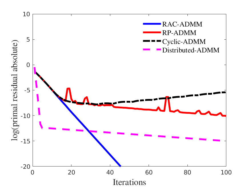
(a) Primal residual

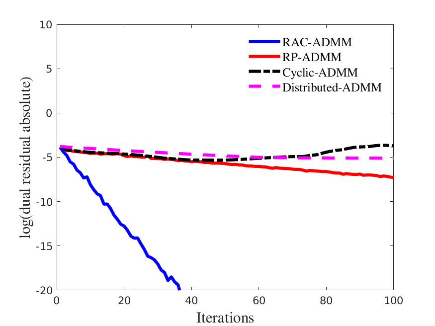
(b) Dual residual

Figure 1: Iteration evolution of primal and dual residuals of ADMM variants

2.2 Convergence of RAC-ADMM

This section concerns with convergence properties of RAC-ADMM when applied to unbounded (i.e. $\operatorname{\mathbf{x}}\in\operatorname{\varmathbb{R}}^{n}$) linearly-equality constrained quadratic optimization problems. To simplify the notation, we use $A=A_{eq}$ and $\operatorname{\mathbf{b}}=\operatorname{\mathbf{b}}_{eq}$.

$${\begin{array}[]{cl}\min\limits_{x}&\frac{1}{2}\operatorname{\mathbf{x}}^{T}H\operatorname{\mathbf{x}}+\operatorname{\mathbf{c}}^{T}\operatorname{\mathbf{x}}\\[8.5359pt] \mbox{s.t.}&A\operatorname{\mathbf{x}}=\operatorname{\mathbf{b}}\end{array}}$$ (9)

with $H\in\operatorname{\varmathbb{R}}^{n\times n},H\succeq 0$, $\operatorname{\mathbf{c}}\in\operatorname{\varmathbb{R}}^{n}$, $A\in\operatorname{\varmathbb{R}}^{m\times n}$, $\operatorname{\mathbf{b}}\in\operatorname{\varmathbb{R}}^{m}$ and $\operatorname{\mathbf{x}}\in\operatorname{\varmathbb{R}}^{n}$.

Convergence analysis of problems that include inequalities (bounds on variables and/or inequality constraints) is still an open question and will be addressed in our subsequent work.

2.2.1 Preliminaries

I) Double Randomness Interpretation

Let $\Gamma_{RAC(n,p)}$ denote all possible updating combinations for RAC with $n$ variables and $p$ blocks, and let $\sigma_{RAC}\in\Gamma_{RAC(n,p)}$ denote one specific updating combination for RAC-ADMM. Then the total number of updating combinations for RAC-ADMM is given by

$${|\Gamma_{RAC(n,p)}|=\dfrac{n!}{(s!)^{p}}}$$

where $s\in\operatorname{\varmathbb{Z}}_{+}$ denotes size of each block with $p\cdot s=n$.

RAC-ADMM could be viewed as a double-randomness procedure based on RP-ADMM with different block compositions. Let $\sigma_{RP}\in\Gamma_{RP(p)}$ denote an updating combinations of RP-ADMM with $p$ blocks where the variable composition in each block is fixed. Clearly, the total number of updating combinations for RP-ADMM is given by

$${|\Gamma_{RP(p)}|=p!}$$

the total number of possible updating orders of the $p$ blocks. Then, one may consider RAC-ADMM first randomly chooses a block composition and then applies RP-ADMM. Let $\upsilon_{i}\in\Upsilon(n,p)$ denote one specific block composition or partition of $n$ decision variables into $p$ blocks, where $\Upsilon(n,p)$ is the set of all possible block compositions. Then, the total number of all possible block compositions is given by

$${|\Upsilon(n,p)|=\dfrac{|\Gamma_{RAC(n,p)}|}{|\Gamma_{RP(p)}|}=\dfrac{n!}{(s!)^{p}p!}}$$

For convenience, in what follows let $\Gamma_{RP(p),\upsilon_{i}}$ denote all possible updating orders with a fixed block composition $\upsilon_{i}$.

To further illustrate the relations of RP-ADMM and RAC-ADMM, consider the following simple example.

Example 2.1.

Let $n=6$, $p=3$, so $|\Gamma_{RP(6,3)}|=3!=6$, and the total number of block compositions or partitions is $15$:

$${\begin{array}[]{cl}\upsilon_{i}\in\Upsilon(6,3)=&\big{\{}\{[x_{1},x_{2}],[x_{3},x_{4}],[x_{5},x_{6}]\},\{[x_{1},x_{2}],[x_{3},x_{5}],[x_{4},x_{6}]\},\{[x_{1},x_{2}],[x_{3},x_{6}],[x_{4},x_{5}]\},\\ &\{[x_{1},x_{3}],[x_{2},x_{4}],[x_{5},x_{6}]\},\{[x_{1},x_{3}],[x_{2},x_{5}],[x_{4},x_{6}]\},\{[x_{1},x_{3}],[x_{2},x_{6}],[x_{4},x_{5}]\},\\ \hbox{}\hfil&\{[x_{1},x_{4}],[x_{2},x_{3}],[x_{5},x_{6}]\},\{[x_{1},x_{4}],[x_{2},x_{5}],[x_{3},x_{6}]\},\{[x_{1},x_{4}],[x_{2},x_{6}],[x_{3},x_{5}]\},\\ \hbox{}\hfil&\{[x_{1},x_{5}],[x_{2},x_{3}],[x_{4},x_{6}]\},\{[x_{1},x_{5}],[x_{2},x_{4}],[x_{3},x_{6}]\},\{[x_{1},x_{5}],[x_{2},x_{6}],[x_{3},x_{4}]\},\\ \hbox{}\hfil&\{[x_{1},x_{6}],[x_{2},x_{3}],[x_{4},x_{5}]\},\{[x_{1},x_{6}],[x_{2},x_{4}],[x_{3},x_{5}]\},\{[x_{1},x_{6}],[x_{2},x_{5}],[x_{3},x_{4}]\}\big{\}}\end{array}}$$

RAC-ADMM could be viewed as if, at each cyclic loop, the algorithm first selects a block composition $\upsilon_{i}$ uniformly random from all possible $15$ block compositions $\Upsilon(n,p)$, and then performs RP-ADMM with the chosen specific block composition $\upsilon_{i}$. In other words, RAC-ADMM then randomly selects $\sigma\in\Gamma_{RP(p),\upsilon_{i}}$, which leads to a total of $90$ possible updating combinations.

II) RAC-ADMM as a linear transformation

Recall that the augmented Lagrangian function for (9) is given by

$${L_{\beta}(\operatorname{\mathbf{x}},\operatorname{\mathbf{y}})=\frac{1}{2}\operatorname{\mathbf{x}}^{T}H\operatorname{\mathbf{x}}+\operatorname{\mathbf{c}}^{T}\operatorname{\mathbf{x}}-\operatorname{\mathbf{y}}^{T}(A\operatorname{\mathbf{x}}-\operatorname{\mathbf{b}})+\frac{1}{2}{\beta}||A\operatorname{\mathbf{x}}-\operatorname{\mathbf{b}}||^{2}.}$$

Consider one specific update order generated by RAC, $\sigma_{RAC}\in\Gamma_{RAC(n,p)}$. Note that we use $\sigma$ instead $\sigma_{RAC}$ when there is no confusion. One possible update combination generated by RAC, $\sigma=[\sigma_{1},\dots,\sigma_{p}]$, where $\sigma_{i}$ is an index vector of size $s$, is as follows,

$${\mbox{RAC-ADMM}_{k+1}=\left\{\begin{array}[]{l}\operatorname{\mathbf{x}}_{\sigma 1}^{k+1}=\operatorname*{arg\,min}\limits_{\operatorname{\mathbf{x}}_{\sigma 1}}\{L_{\beta}(\operatorname{\mathbf{x}}_{\sigma 1},\operatorname{\mathbf{x}}_{\sigma 2}^{k},\dots,\operatorname{\mathbf{x}}_{\sigma p}^{k};\operatorname{\mathbf{y}}^{k})\},\\[-8.5359pt] \vdots\\ \operatorname{\mathbf{x}}_{\sigma p}^{k+1}=\operatorname*{arg\,min}\limits_{\operatorname{\mathbf{x}}_{\sigma p}}\{L_{\beta}(\operatorname{\mathbf{x}}_{\sigma 1}^{k+1},\operatorname{\mathbf{x}}_{\sigma 2}^{k+1},\dots,\operatorname{\mathbf{x}}_{\sigma p};\operatorname{\mathbf{y}}^{k})\},\\[11.38092pt] \operatorname{\mathbf{y}}^{k+1}=\operatorname{\mathbf{y}}^{k}-\beta(A\operatorname{\mathbf{x}}^{k+1}-\operatorname{\mathbf{b}}).\end{array}\right.}$$

For convenience, we follow the notation in [15] and [64, 65] to describe the iterative scheme of RAC-ADMM in a matrix form. Let $L_{\sigma}\in\operatorname{\varmathbb{R}}^{n\times n}$ be $s\times s$ block matrix defined with respect to $\sigma_{i}$ rows and $\sigma_{j}$ columns as

$${(L_{\sigma})_{\sigma_{i},\sigma_{j}}:=\begin{cases}\begin{array}[]{ll}H_{\sigma_{i},\sigma_{j}}+\beta A^{T}_{\sigma_{i}}A_{\sigma_{j}},&\quad i\geq j\\ 0,&\quad\textup{otherwise}\end{array}\end{cases}}$$

and let $R_{\sigma}$ be defined as

$${R_{\sigma}:=L_{\sigma}-(H+\beta A^{T}A).}$$

By setting $\operatorname{\mathbf{z}}:=(\operatorname{\mathbf{x}};\operatorname{\mathbf{y}})$, RAC-ADMM could be viewed as a linear system mapping iteration

$${\operatorname{\mathbf{z}}^{k+1}:=M_{\sigma}\operatorname{\mathbf{z}}^{k}+\bar{L}^{-1}_{\sigma}\bar{\operatorname{\mathbf{b}}}}$$

where

$${M_{\sigma}:=\bar{L}^{-1}_{\sigma}\bar{R}_{\sigma}}$$ (10)

and

$${\begin{array}[]{ccc}\bar{L}_{\sigma}:=\begin{bmatrix}L_{\sigma}&0\\ \beta A&I\end{bmatrix}&\bar{R}_{\sigma}:=\begin{bmatrix}R_{\sigma}&A^{T}\\ 0&I\end{bmatrix}&\bar{\operatorname{\mathbf{b}}}:=\begin{bmatrix}-\operatorname{\mathbf{c}}+\beta A^{T}\operatorname{\mathbf{b}}\\ \beta\operatorname{\mathbf{b}}\end{bmatrix}\end{array}}$$

Define the matrix $Q$ by

$${Q:=\operatorname{\mathbb{E}}_{\sigma}(L^{-1}_{\sigma})=\frac{1}{|\Gamma_{RAC(n,p)}|}\sum\nolimits_{\sigma\in\Gamma_{RAC(n,p)}}L_{\sigma}^{-1}=\frac{1}{|\Upsilon(n,p)|}\sum\nolimits_{\upsilon_{i}\in\Upsilon(n,p)}\left\{\frac{1}{p!}\sum\nolimits_{\sigma\in\Gamma_{RP(p),\upsilon_{i}}}L^{-1}_{\sigma}\right\}}$$

Notice that for any block structure $\upsilon_{i}$ any update order within this fixed block structure $\sigma\in\Gamma_{RP(p),\upsilon_{i}}$, we have $L_{\sigma}^{T}=L_{\bar{\sigma}}$, where $\bar{\sigma}$ is a reverse permutation of $\sigma\in\Gamma_{RP(p),\upsilon_{i}}$. Specifically, let $\sigma=[\sigma_{1},\dots,\sigma_{p}]$, we have $\bar{\sigma}=[\bar{\sigma}_{1},\dots,\bar{\sigma}_{p}]$, and $\bar{\sigma}_{i}=\sigma_{p+1-i}$. For a specific fixed block structure $\upsilon_{i}$, define matrix $Q_{\upsilon_{i}}$ as

$${Q_{\upsilon_{i}}:=\operatorname{\mathbb{E}}(L_{\sigma}|\upsilon_{i})=\frac{1}{p!}\sum\nolimits_{\sigma_{i}\in\Gamma_{RP(n,\upsilon_{i})}}L^{-1}_{\sigma_{i}},}$$

and because $L_{\sigma}^{T}=L_{\bar{\sigma}}$, matrix $Q_{\upsilon_{i}}$ is symmetric for all $i$, and

$${Q:=\frac{1}{\Upsilon(n,p)}\sum\nolimits_{\upsilon_{i}\in\Upsilon(n,p)}Q_{\upsilon_{i}}}$$ (11)

Finally, the expected mapping matrix $M$ is given by

$${M:=\operatorname{\mathbb{E}}_{\sigma}(M_{\sigma})=\frac{1}{|\Gamma_{RAC(n,p)}|}\sum\nolimits_{\sigma\in\Gamma_{RAC(n,p)}}M_{\sigma}}$$

or, by direct computation,

$${M:=\begin{bmatrix}I-QS&QA^{T}\\ -\beta A+\beta AQS&I-\beta AQA^{T}\end{bmatrix}}$$

where $S=H+\beta A^{T}A$.

2.2.2 Expected convergence of RAC-ADMM

With the preliminaries defined, we are now ready to show that RAC-ADMM converges in expectation under the following assumption:

Assumption 2.1.

Assume that for any block of indices $\sigma_{i}$ that generated by RAC-ADMM

$${H_{\sigma_{i},\sigma_{i}}+\beta A^{T}_{\sigma_{i}}A_{\sigma_{i}}\succ 0}$$

where $\sigma_{i}$ is the index vector describing indices of primal variables of the block $i$.

Theorem 2.2.

Suppose that Assumption (2.1) holds, and that RAC-ADMM (8) is employed to solve problem (9). Then the expected output converges to some KKT point of (9).

Theorem 2.2 suggests that the expected output converges to some KKT point of (9). Such convergence in expectation criteria has been widely used in many randomized algorithms, including convergence analysis for RP-BCD and RP-ADMM (e.g. [14, 64]), and stochastic quasi-newton methods (e.g. [10]). It is worth mentioning that if the optimization problem is strictly convex (H¿0), we are able to prove that the expected mapping matrix has specturm that is strictly less than 1, following corollary 2.4.1.

Although convergence in expectation is widely used in many literature, it is still a relatively weak convergence criteria. Thih is why in section 2.2.4 we propose a sufficient condition for almost surely convergence of RAC-ADMM. The section also provides an example showing a problem with $\rho(M)<1$ which does not converge. Rather it oscillates almost surely (Example LABEL:example_diverge). To the best of our knowledge, this is the first example showing that even if a randomized optimization algorithm has expected spectrum radius strictly less than 1, the algorithm may still oscillate – to construct an example with expected spectrum radius equals to 1 that does not converge is an easy task. Consider for example a sequence $\{x_{t},t\geq 0\}$ with $x_{t}=-1$ and $x_{t}=1$, chosen with equal probabilities (prob=1/2). Then, the sequence does not converge with probability 1. However, under the such example, the expected spectrum of this mapping procedure $\rho(M)$ actually equals to 1, which implies that the sequence may not converge.

Despite the fact that such example exists for RAC-ADMM, in all the numerical tests provided in section LABEL:sect:num, RAC-ADMM converges to the KKT point of the optimization problem under few iterations. Such strong numerical evidences imply that in practice, our algorithm does not require taking expectation over many iterations to converge.

The proof of Theorem 2.2 follows the proof structure of [64, 15, 65] to show that under Assumption 2.1:

1. $\operatorname{\hbox{eig}}(QS)\in[0,\frac{4}{3})$ ;

2. $\forall\lambda\in\operatorname{\hbox{eig}}(M),\operatorname{\hbox{eig}}(QS)\in[0,\frac{4}{3})\implies\|\lambda\|<1$ or $\lambda=1$;

3. if $1\in\operatorname{\hbox{eig}}(M)$, then the eigenvalue 1 has a complete set of eigenvectors;

4. Steps (2) and (3) imply the convergence in expectation of the RAC-ADMM.

The proof builds on Theorem 2 from [15], which describes RP-ADMM convergence in expectation under specific conditions put on matrices $H$ and $A$, and Weyl’s inequality, which gives the upper bound on maximum eigenvalue and the lower bound on minimum eigenvalue of a sum of Hermitian matrices. Proofs for items (2) and (3) are identical to proofs given in [15], Section 3.2, so here the focus in on proving item (1).

The following lemma completes the proof of expected convergence of RAC.

Lemma 2.3.

Under assumption 2.1, the matrix $Q$ is positive definite, and

$${eig(QS)\subset[0,\frac{4}{3})}$$

To prove Lemma 2.3, we first show that for any block structure $\upsilon_{i}$, the following proposition holds:

Proposition 2.4.

$Q_{\upsilon_{i}}S$ is positive semi-definite and symmetric, and

$${eig(Q_{\upsilon_{i}}S)\subseteq[0,\frac{4}{3})}$$

Intuitively, a different block structure of RAC-ADMM iteration could be viewed as relabeling variables and performing RP-ADMM procedure as described in [15].

Proof. Define block structure $\{[x_{1},\dots,x_{s}],[x_{s+1},\dots,x_{2s}],[x_{(p-1)s+1},\dots,x_{ps}]\}$ as $\upsilon_{1}$. For any block structure $\upsilon_{i}$, there exists $\tilde{S}$ and $\tilde{Q}_{\upsilon_{1}}$ s.t.

$${\operatorname{\hbox{eig}}(Q_{\upsilon_{i}}S)=\operatorname{\hbox{eig}}(\tilde{Q}_{\upsilon_{1}}\tilde{S})}$$

where $\tilde{Q}_{\upsilon_{1}}$ represents formulation of $\operatorname{\mathbb{E}}_{\sigma}(L_{\sigma}^{-1})$ matrix with respect to block structure $\upsilon_{1}$ and matrix $\tilde{S}$. To prove this, we introduce permutation matrix $P_{\upsilon_{1}\to\upsilon_{i}}$ as follows.

Given

$${\begin{array}[]{ll}\upsilon_{1}=&\{[1,\dots,{s}],[{s+1},\dots,{2s}],[{(p-1)s+1},\dots,{ps}]\}\\ \upsilon_{i}=&\{[\pi(1),\dots,\pi({s})],[\pi({s+1}),\dots,\pi({2s})],[\pi({(p-1)s+1}),\dots,\pi({ps})]\}\end{array}}$$

define

$${P_{\upsilon_{i}}=\begin{bmatrix}\operatorname{\mathbf{e}}_{\pi(1)}\\ \operatorname{\mathbf{e}}_{\pi(2)}\\ \vdots\\ \operatorname{\mathbf{e}}_{\pi(ps)}\end{bmatrix}}$$

Where $\operatorname{\mathbf{e}}_{i}$ is the row vector with $i^{th}$ element equal to 1. Notice $P_{\upsilon_{i}}$ is orthogonal matrix for any $\upsilon_{i}$, i.e. $P_{\upsilon_{i}}P_{\upsilon_{i}}^{T}=I$. For any fixed block structure $\upsilon_{i}$, with an update order within $\sigma_{RP}\in\Gamma_{RP}(p)$, the following equality holds

$${L_{\sigma_{RP},S,\upsilon_{i}}=P_{\upsilon_{i}}^{T}L_{\sigma_{RP},\tilde{S},\upsilon_{1}}P_{\upsilon_{i}}}$$

where $L_{\sigma_{RP},S,\upsilon_{i}}$ is the construction of $L$ following update order $\sigma_{RP}\in\Gamma_{RP}(p)$ and block structure $\upsilon_{i}$ with respect to $S$, and $L_{\sigma_{RP},\tilde{S},\upsilon_{1}}$ is the construction of $L$ following update order $\sigma_{RP}\in\Gamma_{RP}(p)$ and block structure $\upsilon_{1}$, with coefficient matrix $\tilde{S}$, and

$${\tilde{S}=P_{\upsilon_{i}}SP_{\upsilon_{i}}^{T}}$$

and

$${L_{\sigma,S,\upsilon_{i}}^{-1}=(P_{\upsilon_{i}}^{T}L_{\sigma,\tilde{S},\upsilon_{1}}P_{\upsilon_{i}})^{-1}=P_{\upsilon_{i}}^{T}L^{-1}_{\sigma,\tilde{S},\upsilon_{1}}P_{\upsilon_{i}}.}$$

Then by the definition of $Q$ matrix (Eq. 11), we get

$${Q_{\upsilon_{i},S}=P_{\upsilon_{i}}^{T}\tilde{Q}_{\upsilon_{1},\tilde{S}}P_{\upsilon_{i}}}$$

so that

$${Q_{\upsilon_{i},S}S=P_{\upsilon_{i}}^{T}\tilde{Q}_{\upsilon_{1},\tilde{S}}P_{\upsilon_{i}}P_{\upsilon_{i}}^{-1}\tilde{S}P_{\upsilon_{i}}=P_{\upsilon_{i}}^{T}\tilde{Q}_{\upsilon_{1},\tilde{S}}\tilde{S}P_{\upsilon_{i}}.}$$

Considering the eigenvalues of $Q_{\upsilon_{i},S}S$,

$${\operatorname{\hbox{eig}}(Q_{\upsilon_{i},S}S)=\operatorname{\hbox{eig}}(P_{\upsilon_{i}}^{T}\tilde{Q}_{\upsilon_{1},\tilde{S}}\tilde{S}P_{\upsilon_{i}})=\operatorname{\hbox{eig}}(\tilde{Q}_{\upsilon_{1},\tilde{S}}\tilde{S})}$$

and from [15], under Assumption $(\ref{assumption1})$, $\tilde{Q}_{\upsilon_{1},\tilde{S}}$ is positive definite, and

$${eig(\tilde{Q}_{\upsilon_{1},\tilde{S}}\tilde{S})\subset[0,\frac{4}{3})}$$

which implies $Q_{\upsilon_{i}}$ is positive definite, and

$${eig(Q_{\upsilon_{i}}S)\subset[0,\frac{4}{3}).}$$

Notice that by definition of $Q$, we have

$${QS=\frac{1}{\Upsilon(d,n)}\sum_{\upsilon_{i}}Q_{\upsilon_{i}}S}$$

and $Q_{\upsilon_{i}}S$ is positive definite and symmetric. Let $\lambda_{1}(A)$ denote the maximum eigenvalue of matrix $A$, then as all $Q_{\upsilon_{i}}S$ are Hermitian matrices, by Weyl’s theorem, we have

$${\lambda_{1}(QS)=\lambda_{1}(\frac{1}{\Upsilon(d,n)}\sum_{i\in\Upsilon}Q_{\upsilon_{i}}S)\leq\frac{1}{\Upsilon(d,n)}\sum_{i\in\Upsilon}\lambda_{1}(Q_{\upsilon_{i}}S)}$$

and as $\lambda_{1}(Q_{\upsilon_{i}}S)<\frac{4}{3}$ for each $i$,

$${\operatorname{\hbox{eig}}(QS)\subseteq[0,\frac{4}{3})}$$

which completes the proof of Lemma 2.3, and thus establishes that RAC-ADMM is guaranteed to converge in expectation. ∎

When the problem is strongly convex ($H\succ 0$), we introduce the following corollary.

Corollary 2.4.1.

Under assumption 2.1, and $H\succ 0$,

$${\rho(M)<1}$$

Proof. When $H\succ 0$, by definition $S=H+\beta A^{T}A\succ 0$, and by Lemma 2.3, $Q\succ 0$, hence $\operatorname{\hbox{eig}}(QS)\subseteq(0,\dfrac{4}{3})$, and this implies $\rho(M)<1$. ∎ Note that there are random sequences converging in expectation where their spectrum-radius equal to one. Therefore, for solving strongly non-separable convex quadratic optimization, the expected convergence rate of RAC-ADMM is proved to be linear, which result is stronger than just ”convergence in expectation”.

2.2.3 Convergence speed of RAC-ADMM vs. RP-ADMM

Following is a corollary to show that on average or in expectation, RAC-ADMM performs RP-ADMM with a fixed block composition in sense of spectral radius of mapping matrix.

Corollary 2.4.2.

Under Assumption 2.1, with $H=0$ so that $S=\beta A^{T}A$, where $A\in\operatorname{\varmathbb{R}}^{n\times n}$ is a non-singular matrix, there exists some RP-ADMM (with specific block compositions), such that expected spectral radius of RAC-ADMM mapping matrix is (weakly) smaller than expected spectral radius of that of RP-ADMM.

Proof. We prove the corollary in solving linear system with $A$ non singular, with null objective function. In this setup, the expected output converges to the unique primal dual optimal solution to (9).

Notice in this setup, we have

$${\begin{array}[]{l}\lambda\in\operatorname{\hbox{eig}}(M)\Leftrightarrow\tau=\dfrac{(1-\lambda)^{2}}{1-2\lambda}\in\operatorname{\hbox{eig}}(QA^{T}A)\\ \lambda_{\upsilon_{i}}\in\operatorname{\hbox{eig}}(M_{RP,\upsilon_{i}})\Leftrightarrow\tau_{\upsilon_{i}}=\dfrac{(1-\lambda_{\upsilon_{i}})^{2}}{1-2\lambda_{\upsilon_{i}}}\in\operatorname{\hbox{eig}}(Q_{\upsilon_{i}}A^{T}A)\end{array}}$$

By calculation, we could characterize $\lambda$ as roots of quadratic polynomial [65],

$${\lambda_{1}=1-\tau+\sqrt{\tau(\tau-1)},\quad\lambda_{2}=1-\tau-\sqrt{\tau(\tau-1)}.}$$

Suppose corollary doesn’t hold, $\rho(E(M_{RAC}))\geq\rho(\operatorname{\mathbb{E}}(M_{RP,\upsilon_{i}}))$ for all possible block structure. Define $\underline{\tau}_{\upsilon_{i}}$ as the the smallest eigenvalue with respect to $Q_{\upsilon_{i}}S$, and $\bar{\tau}_{\upsilon_{i}}$ as the largest eigenvalue with respect to $Q_{\upsilon_{i}}S$. Similarly, $\underline{\tau}$ as the smallest eigenvalue with respect to $QS$, and $\bar{\tau}$ the largest eigenvalue of $QS$. Consider the following two cases.

Case 1.     $\lambda^{*}=\max_{i}|\lambda_{i}|\in\mathbb{C}\textup{ and }\lambda^{*}\notin\operatorname{\varmathbb{R}}\Leftrightarrow\tau_{\lambda^{*}}<1$, where $\tau_{\lambda^{*}}\in\operatorname{\hbox{eig}}(QS)$ satisfies $\dfrac{(1-\lambda^{*})^{2}}{1-2\lambda^{*}}=\tau_{\lambda^{*}}$.

We have, $\rho(E(M_{RAC}))\geq\rho(\operatorname{\mathbb{E}}(M_{RP,\upsilon_{i}}))\ \forall\ i$, which implies that

$${\sqrt{1-\tau_{\lambda^{*}}}>\max\{\sqrt{1-\tau_{\upsilon_{i}}},\tau_{\upsilon_{i}}-1+\sqrt{\tau_{\upsilon_{i}}(\tau_{\upsilon_{i}}-1)}\}\quad\forall i.}$$

Specifically

$${\sqrt{1-\tau_{\lambda^{*}}}>\sqrt{1-\underline{\tau}_{\upsilon_{i}}}\quad\forall\upsilon_{i},}$$

As $f(x)=\sqrt{1-x}$ is monotone decreasing with respect to $x$, the above implies that

$${\tau_{\lambda^{*}}<\underline{\tau}_{\upsilon_{i}}\quad\forall\upsilon_{i},}$$

and as $\tau_{\lambda^{*}}\geq\underline{\tau}$, the above equation implies

$${\underline{\tau}<\underline{\tau}_{\upsilon_{i}}\quad\forall\upsilon_{i},}$$

which is impossible, as by Weyl’s theorem,

$${\underline{\tau}\geq\dfrac{1}{|\Upsilon(d,b)|}\sum_{i}\underline{\tau}_{\upsilon_{i}}\geq\min_{i}\ \underline{\tau}_{\upsilon_{i}}.}$$

Case 2.     $\lambda^{*}=\max_{i}|\lambda_{i}|\in\operatorname{\varmathbb{R}}\Leftrightarrow\tau_{\lambda^{*}}>1$.

We have $\rho(E(M_{RAC}))\geq\rho(\operatorname{\mathbb{E}}(M_{RP,\upsilon_{i}}))\ \forall i$, what implies that

$${\tau_{\lambda^{*}}-1+\sqrt{\tau_{\lambda^{*}}(\tau_{\lambda^{*}}-1)}>\max\{\sqrt{1-\tau_{\upsilon_{i}}},\tau_{\upsilon_{i}}-1+\sqrt{\tau_{\upsilon_{i}}(\tau_{\upsilon_{i}}-1)}\}\quad\forall i.}$$

Specifically,

$${\tau_{\lambda^{*}}-1+\sqrt{\tau_{\lambda^{*}}(\tau_{\lambda^{*}}-1)}>\tau_{\upsilon_{i}}-1+\sqrt{\tau_{\upsilon_{i}}(\tau_{\upsilon_{i}}-1)}\quad\forall i,\quad\forall\upsilon_{i}.}$$

As $g(x)=x-1+\sqrt{x(x-1)}$ is a monotone increasing function for $x\in[1,\infty)$, the above implies

$${\overline{\tau}\geq\tau_{\lambda^{*}}>\overline{\tau}_{\upsilon_{i}}\quad\forall\upsilon_{i},}$$

which is impossible, as by Weyl’s theorem,

$${\bar{\tau}\leq\dfrac{1}{|\Upsilon(d,b)|}\sum_{i}\bar{\tau}_{\upsilon_{i}}\leq\max_{i}\ \underline{\tau}_{\upsilon_{i}}.}$$

∎

2.2.4 Variance of RAC-ADMM

Convergence in expectation may not be a good indicator of convergence for solving all problems, as there may exist a problem for which RAC-ADMM is not stable or possesses greater variance. In order to give another probabilistic measure on performance of RAC-ADMM, this section introduces convergence almost surely (a.s.) as an indicator of the algorithm convergence. Convergence almost surely as a measure for stability has been used in linear control systems for quite some time, and is based on the mean-square stability criterion for stochastically varying systems [17]. The criterion establishes conditions for asymptotic convergence of covariance of the system states (e.g. variables).

This section builds on those results and establishes sufficient condition for RAC-ADMM to converge almost surely when applied to solve (9). The condition utilizes the Kronecker product of the mapping matrix, which captures the dynamics of the second moments of the random sequences generated by RAC-ADMM algorithm, and the expectation over the products of mapping matrices that provides the bounds on the variance of the distance between the KKT point and the random sequence generated by our algorithm.

Theorem 2.5.

Suppose that Assumption 2.1 holds, and that RAC-ADMM (8) is employed to solve problem (9). Then the output of RAC-ADMM converges almost surely to some KKT point of (9) if

$${\rho(\operatorname{\mathbb{E}}(M_{\sigma}\otimes M_{\sigma}))<1}$$

where $M\otimes M$ is the Kronecker product of $M$ with itself.

Proof. Let $\overline{z}=[\overline{x};\overline{y}]\in\operatorname{\varmathbb{R}}^{N}$ denote the KKT point of (9), then, at $k+1^{th}$ iteration we have

$${(z_{k+1}-\overline{z})=M_{\sigma_{k}}(z_{k}-\overline{z}).}$$

Define $d_{k}=z_{k}-\overline{z}$, and

$${P_{k}=\operatorname{\mathbb{E}}(d_{k}d_{k}^{T}).}$$

There exists a linear operator $\mathcal{T}$ s.t.

$${\operatorname{\hbox{vec}}(P_{k+1})=\mathcal{T}\operatorname{\hbox{vec}}(P_{k})}$$ (12)

where $\operatorname{\hbox{vec}}(\cdot)$ is vectorization of a matrix, and $\mathcal{T}=\operatorname{\mathbb{E}}(M_{\sigma}\otimes M_{\sigma})$, as

$${\operatorname{\hbox{vec}}(P_{k+1})=\operatorname{\hbox{vec}}(\operatorname{\mathbb{E}}(d_{k+1}d_{k+1}^{T}))=\dfrac{1}{|\Upsilon(n,p)|}\sum^{|\Upsilon(n,p)|}_{i=1}\operatorname{\hbox{vec}}(M_{i}\operatorname{\mathbb{E}}(d_{k}d_{k}^{T})M_{i}^{T})=\operatorname{\mathbb{E}}(M_{\sigma}\otimes M_{\sigma})\operatorname{\hbox{vec}}(P_{k})}$$

and $\rho(\operatorname{\mathbb{E}}(M_{\sigma}\otimes M_{\sigma}))<1$ implies $d_{k}\overset{a.s.}{\to}\bm{0}$.

To prove this, let $||\cdot||$ be the Frobenius norm of a matrix, $||A||=\sqrt{\sum^{m}_{i=1}\sum^{n}_{j=1}|a_{ij}|^{2}}$

$${\operatorname{\mathbb{E}}(||d_{k}||^{2})=tr(P_{k})\leq||\operatorname{\hbox{vec}}(P_{k})||^{2}}$$

And by $(\ref{eq:kronecker})$,

$${||\operatorname{\hbox{vec}}(P_{k})||^{2}=||\mathcal{T}\operatorname{\hbox{vec}}(P_{k-1})||^{2}=||\mathcal{T}^{k}\operatorname{\hbox{vec}}(P_{0})||^{2}\leq||\mathcal{T}^{k}||^{2}\cdot||\operatorname{\hbox{vec}}(P_{0})||^{2}}$$

If $\rho(\mathcal{T})<1$, we know that $\mathcal{T}$ is convergent, and there exists $\mu>0$, $0<\gamma<1$, s.t.

$${||\mathcal{T}^{k}||^{2}\leq\mu\gamma^{k},}$$

thus there exists $M$ such that,

$${\sum^{\infty}_{k=0}\operatorname{\mathbb{E}}(||d_{k}||^{2})\leq M\sum^{\infty}_{k=0}\gamma^{k}\leq C<\infty}$$

For any $\epsilon>0$, by Markov inequality we have

$${\sum^{\infty}_{k=0}\operatorname{\mathbb{E}}(||d_{k}||^{2})\leq C\Rightarrow\sum^{\infty}_{k=0}\operatorname{\hbox{Prob}}(||d_{k}||^{2}>\epsilon)<\infty,}$$

and as $\sum^{\infty}_{k=0}\operatorname{\hbox{Prob}}(||d_{k}||^{2}<\epsilon)<\infty$, by Borel-Cantelli, and $||d_{k}||^{2}\in m\mathcal{F}_{+}$,

$${d_{k}\overset{a.s.}{\to}\bm{0}\quad\textup{as }k\to\infty}$$

which then implies that randomized ADMM converges almost surely. ∎

To illustrate the stability issues with RAC-ADMM, consider the following example.

For the instances for which the optimal solution remains unknown (e.g. QAPLIB and GSET instances), we use the best known results from the literature. Note that for maximization problems (e.g. Max-Cut, Max-Bisection) gap is the negative of (LABEL:eq:gap). All binary problems are solved with primal residual equal to zero (i.e. the solutions are feasible and integer).

4.2.1 Randomness Helps

We start the analysis of RACQP for binary problems with a shorth example showing that having blocks that are randomly constructed at each iteration, as done by RAC-ADMM, is the main feature that makes RACQP work well for combinatorial problems, without a need for any special adaptation of the algorithm for the discrete domain.

RAC-ADMM can be easily adapted to execute classical ADMM or RP-ADMM algorithms, so here we compare these three ADMM variants when applied to combinatorial problems. We use a small size problem ($n=1000$) and construct a problem using (LABEL:eq:randomGen) applied to problem of Markowitz type (32),

$${\begin{array}[]{cl}\min\limits_{\operatorname{\mathbf{x}}}&\operatorname{\mathbf{x}}^{T}V\operatorname{\mathbf{x}}+\tau\operatorname{\mathbf{m}}^{T}\operatorname{\mathbf{x}}+\kappa\|\operatorname{\mathbf{x}}\|^{2}_{2}\\[8.5359pt] \mbox{s.t.}&\operatorname{\mathbf{e}}^{T}\operatorname{\mathbf{x}}=r\\[5.69046pt] &\operatorname{\mathbf{x}}\in\{0,1\}^{n}\end{array}}$$ (32)

with $\kappa=10^{-5}$ and a positive integer number $r\in\operatorname{\varmathbb{Z}}_{+}$, $r\in(1,n)$ that defines how many stocks from a given portfolio must be chosen. For completeness of the comparison, we implemented distributed-ADMM (Eq. 4) for binary problems and ran the algorithm on the same data.

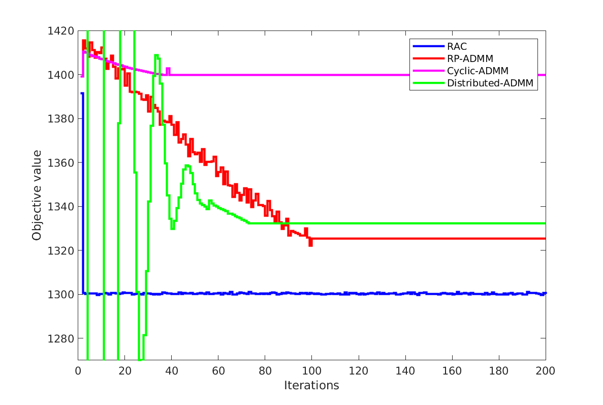
Figure 3: A typical evaluation of the objective function value of (32): RAC-ADMM, RP-ADMM (5), Cyclic ADMM (2) and Distributed ADMM (4)

Results show that RAC-ADMM is much better suited for binary optimization problems than either cyclic ADMM or RP-ADMM or distributed-ADMM, which is not surprising since more randomness is adapted into the algorithm making it more likely to escape local optima. All the algorithms are quick to find a local optimum, but besides RAC-ADMM stay at that first found point, while RAC-ADMM continues to find local optima, which could be better or worse than previously found. Because of this behavior, one can keep track the best solution found ($\operatorname{\mathbf{x}}_{best}$, Algorithm LABEL:alg:RACQP:mip). The algorithms seem robust with respect to the structure of the Hessian and choice of initial point. A typical evaluation of the algorithms is shown in Figure 3. Note that distributed-ADMM has a very low objective value in early iterations, which is due to the large feasibility errors.

4.2.2 Markowitz Portfolio Selection

Similarly to the section on continuous problems, we compare RACQP performance with that of Gurobi on Markowitz cardinality constrained portfolio selection problem (32) using real data coming from CRSP 2018 [74]. In the experiments, we set $r=n/2$ with all other settings identical to those used in Section LABEL:subsect:num:cont:markov, including $V$ and $\operatorname{\mathbf{m}}$, estimated from CRSP 2018 data. The default perturbation RACQP settings with $\beta=0.05$, $p=100$ were used in the experiments. Gap is measured from the “Optimal” objective values of the solutions found by Gurobi in about 1 hour run-time after relaxing MIPGAP parameter to 0.1.

CRSP 2018	Problem	Optimal	Gap
data	size ($n$)	Obj. Val.	run time = 1 min		run time = 5 min		run time = 10 min
			Gurobi∗	RACQP	Gurobi	RACQP	Gurobi	RACQP
quarterly	7958	0.055	36.8	2.0$\cdot$10-3	0	9.0$\cdot$10-4	0	9.0$\cdot$10-4
monthly	7958	0.144	25.9	1.1$\cdot$10-2	-8.7$\cdot$10-6	2.0$\cdot$10-3	-8.7$\cdot$10-6	2.0$\cdot$10-3
daily	4628	1.164	2.9	2.8$\cdot$10-4	0	4.6$\cdot$10-5	0	0

• Root relaxation step not finished. Gurobi returned a heuristic feasible solution.

Table 16: Markowitz portfolio selection model (32). CRSP 2018 data [74].

From the results (Table 16) it is noticeable that RACQP finds relatively good solutions (gap $10^{-2}-10^{-4}$) in a very short time, in some cases even before Gurobi had time to finalize root relaxation step of its binary optimization procedure. Maximal allowed run-time of 1 min was far too short for Gurobi to find any solution, so it returned a heuristic ones. Note that those solutions (third column of the table) are extremely weak, suggesting that a RAC-ADMM based solution could be implemented and used instead.

Low-rank Markowitz portfolio selection model

Similarly to (LABEL:eq:mark:cont2) we formulate the model for low-rank covariance matrix $V$ as

$${\begin{array}[]{cl}\min\limits_{\operatorname{\mathbf{x}}}&\|\operatorname{\mathbf{y}}\|^{2}_{2}-\tau\operatorname{\mathbf{m}}^{T}\operatorname{\mathbf{x}}+\kappa\|\operatorname{\mathbf{x}}\|^{2}_{2}\\[8.5359pt] \mbox{s.t.}&\operatorname{\mathbf{e}}^{T}\operatorname{\mathbf{x}}=r\\[5.69046pt] &B\operatorname{\mathbf{x}}-\operatorname{\mathbf{y}}=\bm{0}\\[5.69046pt] &\operatorname{\mathbf{x}}\in\{0,1\}^{n}\end{array}}$$ (33)

and solve the model for CRSP 2018 data. We use $\beta=0.5$, $p=50$. RACQP gap was measured from the optimal solution returned by Gurobi. In Table 17 we report on the best solutions found by RACQP with max run-time limited to 60 seconds. Results are hard to compare. When Hessian is diagonal and the number of constraints are small, as the case for this data, Gurobi has a very easy time solving the problems (monthly and daily data) – it finds good heuristic points to start with, and solves problems at a root node after a couple of hundreds of simplex iterations. On the other hand, RACQP, which does not directly benefit from diagonal Hessian, needs to execute multiple iterations of ADMM. Even though the problems are small and solved very quickly, the overhead of preparing the sub-problems and initializing Gurobi to solve sub-problems accumulates to the point of overwhelming RACQP run-time. In that light, for the rest of this section we consider problems where Hessian is a non-diagonal matrix, and address the problems that are hard to solve directly by Gurobi (and possibly other MIP QP solvers).

CRSP 2018	Problem	Optimal	Gap
data	size ($n$)	Obj. Val.	Gurobi	RACQP
quarterly	7958	0.015	-2.2$\cdot$10-7	1.6$\cdot$10-3
monthly	7958	0.104	-4.2$\cdot$10-6	-1.3$\cdot$10-5
daily	4628	1.140	3.3	-1.0$\cdot$10-2

Table 17: Low-rank reformulation Markowitz portfolio selection model (32). CRSP 2018 data [74]. Max run-time 1 min.

4.2.3 QAPLIB

The binary quadratic assignment problem (QAP) is known to be NP-hard and that binary instances of larger sizes (dimension of the permutation matrix $r>40$) are considered to be intractable and cannot be solved exactly (though some instances of a large size with special structure have been solved). Currently, the only practical solutions for solving large QAP instances are heuristic methods.

For binary QAP we apply the same method for variance reduction as we did for relaxed QAP (Section LABEL:subsect:qap_relaxed). We group variables following the structure of constraints, which is dictated by the permutation matrix $X\in\{0,1\}^{r\times r}$ (see Eq. LABEL:eq:qaplib:bin for QAP problem formulation) – we construct one super-variable, $\operatorname{\mathbf{x}}_{i}$ for each row $i$ of $X$. Next we make the use of the partial Lagrangian, and split constraints into the local constraint set consisting of (LABEL:eq:qaplib:bin) (a) and the global constraint set consisting of (LABEL:eq:qaplib:bin) (b), so that the partial Lagrangian is

$${L_{\beta}(\operatorname{\mathbf{x}},y)=\frac{1}{2}\operatorname{\mathbf{x}}^{T}H\operatorname{\mathbf{x}}-\operatorname{\mathbf{y}}^{T}(A_{global}\operatorname{\mathbf{x}}-\operatorname{\mathbf{1}})+\frac{\beta}{2}||A_{global}\operatorname{\mathbf{x}}-\operatorname{\mathbf{1}}||^{2}.}$$

At each iteration, we update the $i^{th}$ block by solving ${\operatorname{\mathbf{x}}_{i}^{k+1}=\operatorname*{arg\,min}\{L_{\beta}(\cdot)|\,A_{local}\operatorname{\mathbf{x}}_{i}=\operatorname{\mathbf{1}},\allowbreak\ \operatorname{\mathbf{x}}_{i}\in\{0,1\}^{n}\}.}$ Next, continuing on the discussion on perturbation from the previous section, we turn the feature on and set parameters as follows: number of super-variables to perturb is drawn from truncated exponential distribution, $N_{p}\sim\hbox{Exp}(\lambda)$ with parameter $\lambda=0.4r$, minimum number of variables $N_{p,\hbox{min}}=2$ and maximum number of variables $N_{p,\hbox{max}}=r$. The number of trials before perturbation $N_{trial}$ is set to its default value.

Note that we do not perturb single variables ($x_{i,j}$), rather super-variables that we choose at random. If a super-variable $\operatorname{\mathbf{x}}_{i}$ has value of ’1’ at one location, and ’0’ on all other entries, then we randomly swap location of ’1’ within the super variable (thus keeping the row-wise constraint on $X$ for row $i$ satisfied). If the super-variable is not feasible (number of ’1’$\not=1$), we flip values of a random number of variables that make $\operatorname{\mathbf{x}}_{i}$. The initial point is a random feasible vector. The penalty parameter is a function of the problem size, $\beta=n$, while the number of blocks depends on the permutation matrix size and it is $p=\lceil r/2\rceil$.

QAPLIB [9] benchmark results summary	Gurobi	RACQP
Num. instances opt/best found	3	18
Num. instances gap $<0.01$ (excluding opt/best)	0	17
Num. instances gap $<0.1$ (excluding opt/best and $<0.01$)	3	70

Table 18: Number of instances = 133. Max run-time: 10 min

The summary of the QAPLIB benchmark [57] results is given in Table 18. Out of 133 total instances the benchmark includes, RACQP found the optimal solution (or the best known from literature as not all instances have proven optimal solution) for 18 instances within 10 min of run-time. For the rest of the instances, RACQP returned solutions with an average gap of $\mu=0.07$. Gurobi solved only three instances to optimality. The average gap of the unsolved instances is $\mu=12.15$, which includes heuristic solutions returned when root relaxation step was not finalized (20 instances). Removing those outliers results in the average gap of $\mu=5.57$.

Instance	Problem	Density	Best known	Gap
name	size($n$)	($H$)	Obj val	Gurobi	RACQP
				10 min	5 min	10 min
lipa80a	6400	0.96	253195	0.15∗	0.02	0.01
lipa80b	6400	0.96	7763962	-0.96∗	0.23	0.23
lipa90a	8100	0.97	360630	0.22∗	0.01	0.01
lipa90b	8100	0.97	12490441	-0.96∗	0.23	0.23
sko81	6561	0.69	90998	1.11∗	0.02	0.02
sko90	8100	0.68	115534	1.17∗	0.04	0.03
sko100a	10000	0.68	152002	1.34∗	0.05	0.04
sko100b	10000	0.68	153890	1.38∗	0.04	0.03
sko100c	10000	0.67	147862	1.21∗	0.04	0.03
sko100d	10000	0.67	149576	1.21∗	0.04	0.04
sko100e	10000	0.67	149150	1.17∗	0.05	0.03
sko100f	10000	0.67	149036	1.18∗	0.04	0.03
tai80a	6400	0.96	13499184	-0.98∗	0.06	0.05
tai80b	6400	0.43	818415043	-1.00	0.26	0.22
tai100a	10000	0.96	21043560	-0.97∗	0.06	0.05
tai100b	10000	0.43	1185996137	-1.00∗	0.21	0.21
tai150b	22500	0.44	498896643	-1.00∗	0.21	0.20
tho40	1600	0.38	240516	-0.92	0.04	0.03
tho150	22500	0.42	8133398	-0.89∗	0.08	0.06
wil50	2500	0.86	48816	0.53	0.01	0.01
wil100	10000	0.88	273038	1.19	0.03	0.02

• Root relaxation step not finished. Gurobi returned a heuristic feasible solution.

Table 19: QAPLIB, large problems. Gap between best known results [9, 50] and RACQP/Gurobi objective values.

Table 19 gives detailed information on 21 large instances from QAPLIB data set. The most important takeaway from the table is that Gurobi can not even start solving very large problems as it can not finalize the root relaxation step within given maximum run time, while RACQP can.

4.2.4 Maximum Cut Problem

The maximum-cut (Max-Cut) problem consists of finding a partition of the nodes of a graph $G=(V,E)$, into two disjoint sets $V_{1}$ and $V_{2}$ ($V_{1}\cap V_{2}=\emptyset$, $V_{1}\cup V_{2}=V$) in such a way that the total weight of the edges that have one endpoint in $V_{1}$ and the other in $V_{2}$ is maximized. The problem has numerous important practical applications, and is one of Karp’s 21 NP-complete problems. A standard formulation of the problem is ${\max\limits_{\operatorname{\mathbf{y}}_{i}\in\{-1,1\}}\frac{1}{4}\sum_{i,j}w_{i,j}(1-y_{i}y_{j})}$, which can be re-formulated into quadratic unconstrained binary problem

$${\begin{array}[]{cl}\min\limits_{\operatorname{\mathbf{x}}}&\operatorname{\mathbf{x}}^{T}H\operatorname{\mathbf{x}}\\[5.69046pt] \mbox{s.t.}&\operatorname{\mathbf{x}}\in\{0,1\}^{n}\end{array}}$$ (34)

where $h_{i,j}=w_{i,j}$ and $h_{i,i}=-\frac{1}{2}(\sum_{j=1}^{n}w_{i,j}+\sum_{j=1}^{n}w_{j,i})$.

We use the Gset benchmark from [31], and compare the results of our experiments with the optimal solutions (found by Gurobi) and the best known solutions from the literature [3, 46]. For perturbation we use default parameters and perform perturbation by choosing a random number of variables and negating their values, i.e. $x_{i}=1-x_{i}$. The number of blocks is equal for all instances, $p=4$, and the initial point is set to zero ($\operatorname{\mathbf{x}}_{0}=\operatorname{\mathbf{0}}$) for all the experiments. Note that as the max-cut problem is unconstrained, the enalty parameter $\beta$ is not used (and RACQP is doing a randomly assembled cyclic BCD).

Instance	Problem	Density	Best known	Gap
name	size($n$)	($H$)	Obj val	run time = 5 min		run time = 10 min		run time = 30 min		run time = 60 min
				Gurobi	RACQP	Gurobi	RACQP	Gurobi	RACQP	Gurobi	RACQP
G1	800	6.1$\cdot 10^{-2}$	11624	-0.006	-0.003	-0.005	-0.003	-0.005	-0.002	-0.005	-0.002
G6	800	6.1$\cdot 10^{-2}$	2178	-0.015	-0.011	-0.014	-0.011	-0.012	-0.008	-0.012	-0.008
G11	800	5.8$\cdot 10^{-3}$	564	0	-0.004	0	-0.004	0	-0.004	0	-0.004
G14	800	1.5$\cdot 10^{-2}$	3064	-0.021	-0.001	-0.021	-0.001	-0.021	-0.001	-0.020	-0.001
G18	800	1.5$\cdot 10^{-2}$	992	-0.081	-0.011	-0.081	-0.011	-0.081	-0.011	-0.081	-0.011
G22	2000	1.1$\cdot 10^{-2}$	13359	-0.062	-0.008	-0.062	-0.008	-0.052	-0.008	-0.052	-0.007
G27	2000	1.1$\cdot 10^{-2}$	3848	-0.157	-0.152	-0.155	-0.152	-0.152	-0.151	-0.149	-0.141
G32	2000	2.3$\cdot 10^{-3}$	1410	0	-0.014	0	-0.014	0	-0.014	0	-0.013
G36	2000	6.4$\cdot 10^{-3}$	7678	-0.026	-0.004	-0.026	-0.004	-0.026	-0.004	-0.026	-0.004
G39	2000	6.3$\cdot 10^{-3}$	2408	-0.102	-0.011	-0.102	-0.010	-0.102	-0.006	-0.102	-0.006
G43	1000	2.1$\cdot 10^{-2}$	6660	-0.046	-0.002	-0.046	-0.002	-0.045	-0.002	-0.045	-0.002
G50	3000	1.7$\cdot 10^{-3}$	5880	0	-0.001	0	-0.001	0	-0.001	0	-0.001
G51	1000	1.3$\cdot 10^{-2}$	3848	-0.021	-0.008	-0.021	-0.003	-0.021	-0.003	-0.021	-0.003
G55	5000	1.2$\cdot 10^{-3}$	10299	-0.044	-0.007	-0.041	-0.005	-0.039	-0.005	-0.038	-0.005
G56	5000	1.2$\cdot 10^{-3}$	4016	-0.112	-0.016	-0.112	-0.015	-0.112	-0.011	-0.112	-0.011
G58	5000	2.6$\cdot 10^{-3}$	19276	-0.054	-0.008	-0.040	-0.007	-0.039	-0.005	-0.039	-0.004
G60	7000	8.4$\cdot 10^{-4}$	14187	-0.120	-0.008	-0.098	-0.007	-0.096	-0.005	-0.091	-0.004
G61	7000	8.1$\cdot 10^{-4}$	5796	-0.222	-0.015	-0.181	-0.013	-0.158	-0.013	-0.117	-0.012
G63	7000	1.8$\cdot 10^{-3}$	26997	-0.046	-0.007	-0.046	-0.006	-0.032	-0.005	-0.032	-0.005
G67	10000	4.6$\cdot 10^{-4}$	6940	-0.003	-0.018	-0.002	-0.016	0.001	-0.014	0.001	-0.013
G70	10000	2.8$\cdot 10^{-4}$	9581	-0.006	-0.006	-0.006	-0.006	-0.005	-0.004	-0.004	-0.004
G77	14000	3.3$\cdot 10^{-4}$	9926	-0.016	-0.017	-0.010	-0.017	0.001	-0.013	0.001	-0.012
G81	20000	2.3$\cdot 10^{-4}$	14030	-0.119	-0.023	-0.031	-0.017	-0.023	-0.014	0.002	-0.014
	Average:			-0.0635	-0.0151	-0.0546	-0.0141	-0.0505	-0.0128	-0.0466	-0.0126

Table 20: Max-Cut, GSET instances. Gap between best known results and RACQP/Gurobi objective values.

In contrast to continuous sparse problems (rule 4, Section LABEL:sect:racqp_rules), sparse binary problems benefit from using a randomized multi-block approach, as shown in Table 20. The table compares RACQP and Gurobi results collected from experiments on Gset instances for three different maximum run-time limit settings, 10, 30 and 60 minutes. RACQP again outperforms Gurobi, overall, it finds better solutions when run-time is limited. Although Gurobi does better on a few problems, on average RACQP is better. Note that for large(r) problems ($n\geq 5000$) RACQP keeps improving, which can be explained by the difference in number of perturbations – for smaller problems, good points have already being visited and a chance to find a better one are small. Adaptively changing perturbation parameters could help, but this topic is out of scope of this work.

4.2.5 Maximum Bisection Problem

The maximum bisection problem is a variant of the Max-Cut problem that involves partitioning the vertex set $V$ of a graph $G=(V,E)$ into two disjoint sets $V_{1}$ and $V_{2}$ of equal cardinality (i.e. $V_{1}\cap V_{2}=\emptyset$, $V_{1}\cup V_{2}=V$, $|V_{1}|=|V_{2}|$) such that the total weight of the edges whose endpoints belong to different subsets is maximized. The problem formulation follows (34) with the addition of a constraint $\operatorname{\mathbf{e}}^{T}\operatorname{\mathbf{x}}=\lfloor n/2\rfloor$, where $n$ is the graph size.

For Max-Bisection, at each iteration we would update the $i^{th}$ block by solving

$${\operatorname{\mathbf{x}}_{\omega_{i}}^{k+1}=\operatorname*{arg\,min}\{\operatorname{\mathbf{x}}_{\omega_{i}}^{T}H_{\omega_{i}}\operatorname{\mathbf{x}}_{\omega_{i}}-y(\operatorname{\mathbf{e}}^{T}\operatorname{\mathbf{x}}_{\omega_{i}}-b_{\omega_{i}})+\frac{\beta}{2}\|\operatorname{\mathbf{e}}^{T}\operatorname{\mathbf{x}}_{\omega_{i}}-b_{\omega_{i}}\|^{2}\ |\operatorname{\mathbf{x}}_{\omega_{i}}\in\{0,1\}^{d_{i}}\}}$$

where $d_{i}$ is the size of block $i$, $\operatorname{\mathbf{x}}_{\omega_{i}}$ is a sub-vector of $\operatorname{\mathbf{x}}$ constructed of components of $\operatorname{\mathbf{x}}$ with indices $\omega_{i}\in\Omega$, and $b_{\omega_{i}}=\lfloor n/2\rfloor-\operatorname{\mathbf{e}}^{T}\operatorname{\mathbf{x}}_{-\omega_{i}}$ with $\operatorname{\mathbf{x}}_{-\omega_{i}}$ being the sub-vector of $\operatorname{\mathbf{x}}$ with indices not chosen by $\omega_{i}$. Solving the sub-problems directly has shown to be very time consuming. However, noticing that Gurobi, while solving the problem as whole, makes a good use of cuts for this type of problems (matrix Q structure), we decided to reformulate the sub-problems as follows

$${\begin{array}[]{cl}\min\limits_{\operatorname{\mathbf{x}}}&\operatorname{\mathbf{x}}_{\omega_{i}}^{T}H_{\omega_{i}}\operatorname{\mathbf{x}}_{\omega_{i}}-yr+\frac{\beta}{2}r^{2}\\[5.69046pt] \mbox{s.t.}&\operatorname{\mathbf{e}}^{T}\operatorname{\mathbf{x}}_{\omega_{i}}-r=\operatorname{\mathbf{b}}_{\omega_{i}}\\[5.69046pt] &\operatorname{\mathbf{x}}_{\omega_{i}}\in\{0,1\}^{d_{i}},\ r\in\{0,1\}.\end{array}}$$

Note that $r$ can be also defined as a bounded continuous or integer variable, but because the optimal value is zero and because Gurobi makes good use of binary cuts, we decided to define $r$ as binary.

As in the previous section, we use Gset benchmark library and compare the results of our experiments with the best known solutions for max-bisection problems found in the literature [46]. The experimental setup is identical to that of Max-Cut experiments except for the use of the penalty parameter $\beta=0.005$ and the initial point $\operatorname{\mathbf{x}}_{0}$ which is a feasible random vector. Perturbation is done with a simple swap – an equal number of variables with values “1” and “0” is chosen and the new value set to be the negation of the old value.

Instance	Problem	Density	Best known	Gap
name	size($n$)	($H$)	Obj val	run time = 5 min		run time = 10 min		run time = 30 min		run time = 60 min
				Gurobi	RACQP	Gurobi	RACQP	Gurobi	RACQP	Gurobi	RACQP
G1	800	6.1$\cdot 10^{-2}$	11624	-0.004	-0.005	-0.004	-0.005	-0.004	-0.005	-0.002	-0.001
G6	800	6.1$\cdot 10^{-2}$	2177	-0.023	-0.004	-0.022	-0.003	-0.018	-0.003	-0.015	-0.003
G11	800	5.8$\cdot 10^{-3}$	564	0	-0.014	0	-0.011	0	-0.007	m	-0.007
G14	800	1.5$\cdot 10^{-2}$	3062	-0.019	-0.008	-0.019	-0.008	-0.019	-0.002	-0.018	-0.002
G18	800	1.5$\cdot 10^{-2}$	992	-0.062	-0.004	-0.062	-0.004	-0.062	-0.001	-0.062	-0.001
G22	2000	1.1$\cdot 10^{-2}$	13359	-0.207	-0.009	-0.207	-0.005	-0.171	-0.003	-0.066	-0.003
G27	2000	1.1$\cdot 10^{-2}$	3341	-0.050	-0.023	-0.050	-0.021	-0.043	-0.016	-0.042	-0.014
G32	2000	2.3$\cdot 10^{-3}$	1410	0	-0.010	0	-0.010	0	-0.009	m	-0.009
G36	2000	6.4$\cdot 10^{-3}$	7678	-0.021	-0.004	-0.021	-0.004	-0.021	-0.004	-0.021	-0.004
G39	2000	6.3$\cdot 10^{-3}$	2408	-0.088	-0.011	-0.073	-0.010	-0.072	-0.010	-0.072	-0.010
G43	1000	2.1$\cdot 10^{-2}$	6659	-0.075	-0.004	-0.059	-0.004	-0.057	-0.001	-0.057	-0.001
G50	3000	1.7$\cdot 10^{-3}$	5880	-0.012	0.000	-0.012	0.000	-0.004	0.000	-0.004	0.000
G51	1000	1.3$\cdot 10^{-2}$	3847	-0.017	-0.005	-0.015	-0.005	-0.015	-0.004	-0.014	-0.004
G55	5000	1.2$\cdot 10^{-3}$	10299	-0.120	-0.008	-0.041	-0.007	-0.040	-0.006	-0.038	-0.006
G56	5000	1.2$\cdot 10^{-3}$	4016	-0.197	-0.019	-0.109	-0.018	-0.098	-0.017	-0.089	-0.017
G58	5000	2.6$\cdot 10^{-3}$	19276	-0.169	-0.007	-0.169	-0.007	-0.037	-0.005	-0.037	-0.005
G60	7000	8.4$\cdot 10^{-4}$	14187	-0.166	-0.011	-0.136	-0.006	-0.074	-0.004	-0.074	-0.004
G61	7000	8.1$\cdot 10^{-4}$	5796	-0.359	-0.019	-0.359	-0.019	-0.180	-0.019	-0.167	-0.018
G63	7000	1.8$\cdot 10^{-3}$	26988	-0.226	-0.007	-0.158	-0.006	-0.128	-0.004	-0.038	-0.003
G67	10000	4.6$\cdot 10^{-4}$	6938	-0.258	-0.016	-0.173	-0.014	-0.004	-0.011	-0.001	-0.010
G70	10000	2.8$\cdot 10^{-4}$	9581	-0.009	-0.008	-0.009	-0.006	-0.008	-0.004	-0.004	-0.003
G77	14000	3.3$\cdot 10^{-4}$	9918	-0.468	-0.015	-0.468	-0.013	-0.211	-0.012	-0.015	-0.010
G81	20000	2.3$\cdot 10^{-4}$	14030	-0.280	-0.017	-0.280	-0.015	-0.253	-0.014	-0.127	-0.012
	Average:			-0.1348	-0.0099	-0.1165	-0.0087	-0.0722	-0.0070	-0.0459	-0.0064

Table 21: Max-Bisection, GSET instances. Gap between best known results and RACQP/Gurobi objective values.

The results are shown in Table 21. Compared to the unconstrained max-cut problem, RACQP seems to have less trouble solving max-bisection problem – adding a single constraint boosted its performance by up to 2x. Gurobi performance on the other worsened. Overall, RACQP outperforms Gurobi, finding better solutions when run-time is limited. Both Gurobi and RACQP continue gaining on solution quality (gap gets smaller) with longer time limits.

4.3 Selected Machine Learning Problems

In this section we apply RAC method and RP method to few selected machine learning (ML) problems related to convex quadratic optimization, namely Linear Regression (Elastic-Net) and Support Vector Machine (SVM). To solve the former we apply a specialized implementation of RAC-ADMM (available for download at [58]), while for the latter we use RACQP solver.

4.3.1 Linear Regression using Elastic Net

For a classical linear regression model, with observed features ${\mathbf{X}\in\mathbb{R}^{n\times p}}$, where $n$ is number of observations and $p$ is number of features, one solves the following unconstrained optimization problem

$${\min_{\beta}\ \frac{1}{2n}(y-\mathbf{X}\beta)^{\prime}(y-\mathbf{X}\beta)+P_{\lambda,\alpha}(\beta)}$$ (35)

with ${P_{\lambda,\alpha}(\beta)=\lambda\{\frac{1-\alpha}{2}\|\beta\|_{2}+\alpha\|\beta\|_{1}\}}$ used for Elastic Net model. By adjusting $\alpha$ and $\lambda$, one could obtain different models: for ridge regression, $\alpha=0$, for lasso $\alpha=1$, and for classic linear regression, $\lambda=0$. For the problem to be solved by ADMM, we use variable splitting and reformulate the problem as follows

$${\begin{array}[]{rccl}\begin{array}[]{cl}\min\limits_{\beta}&\frac{1}{2N}(y-X\beta)^{T}(y-X\beta)+P_{\lambda,\alpha}(z)\\ \mbox{s.t.}&\beta-\operatorname{\mathbf{z}}\ =\ \operatorname{\mathbf{0}}\end{array}\end{array}}$$ (36)

Note that in (36) we follow the standard machine learning Elastic Net notation in which $\beta$ is the decision variable in the optimization formulation, rather than $\operatorname{\mathbf{x}}$.

Let $c=-\frac{1}{n}X^{T}y$, $A=\frac{X}{\sqrt{n}}$, and let $\gamma$ denote the augmented Lagrangian penalty parameter with respect to constraint $\beta-z$, and $\xi$ be the dual with respect to constraint $\beta-z$. The augmented Lagrangian could then be written as

$${\begin{array}[]{ll}L_{\lambda}=&\frac{1}{2}\beta^{T}(A^{T}A+\gamma I)\beta+(c-\xi)^{T}\beta+(\xi-\gamma\beta)^{T}z+\frac{\gamma}{2}z^{T}z+P_{\lambda,\alpha}(z)\end{array}}$$

We apply RAC-ADMM algorithm by partitioning $\beta$ into multi-blocks, but solve $z$ as one block. For any given $\beta_{k+1}$, optimizer $z^{*}_{k+1}$ has the closed form solution.

$${z^{*}_{k+1}(i)(\beta_{k+1}(i),\xi_{k}(i))=\frac{S(\xi_{k}(i)-\gamma\beta_{k+1}(i),\lambda\alpha)}{(1-\alpha)\lambda+\gamma},}$$

where $\xi_{i}$ is the dual variable with respect to constraint $\beta_{i}-z_{i}=0$, and $S(a,b)$ is soft-threshold operation [27].

$${S(a,b)=\begin{cases}-(a-b),&\textup{if}\ b<|a|,\ a>0\\ -(a+b),&\textup{if}\ b<|a|,\ a\leq 0\\ 0,&\textup{if}\ b\geq|a|\\ \end{cases}}$$

In order to solve classic linear regression directly, $\mathbf{X}^{T}\mathbf{X}$ must be positive definite which can not be satisfied for $p>n$. However, RAC-ADMM only requires each sub-block $\mathbf{X}_{sub}^{T}\mathbf{X}_{sub}$ to be positive definite, so, as long as block size $s<n$, RAC-ADMM can be used to solve the classic linear regression.

We compare our solver with glmnet [28, 60] and Matlab lasso implementation on synthetic data (sparse and dense problems) and benchmark regression data from LIBSVM [12].

Synthetic Data

The data set for dense problems $\mathbf{X}$ is generated uniform randomly with $n=10,000$, $p=50,000$, with zero sparsity, while for the ground truth $\beta^{*}$ we use standard Gaussian and set sparsity of $\beta^{*}$ to $0.1$. Due to the nature of the problem, estimation requires lower feasibility precision, so we fix number of iterations to $10$ and $20$. Glmnet solver benefits from having a diminishing sequence of $\lambda$, but given that many applications (e.g. see [2]) require a fixed $\lambda$ value , we decided to use fixed $\lambda$ for all solvers. Note that the computation time of RAC-ADMM solver is invariant regardless of whether $\lambda$ is decreasing or fixed.

$\lambda$	Num.	Absolute L2 loss				Total time [s]
	iterations	RAC	RP	glmnet	Matlab	RAC	RP	glmnet	Matlab
0.01	10	204.8	204.6	213.9	249.1	396.5	227.6	2465.9	1215.2
	20	208.1	230.2	213.9	237.1	735.2	343.9	3857.9	2218.2
0.1	10	217.8	215.6	220.5	213.1	388.7	212.5	4444.3	2125.9
	20	272.6	202.4	220.5	212.4	739.7	337.2	4452.4	2434.6
1	10	213.6	209.0	203.1	210.5	415.3	213.6	3021.1	1138.9
	20	213.8	212.4	210.5	203.1	686.3	392.1	5295.5	1495.6

Table 22: Comparison on solver performance, dense elastic net model. Dense problem, $n=10,000,\ p=50,000$

Table 22 reports on the average cross-validation run-time and the average absolute $L2$ loss for all possible pairs $(\alpha,\lambda)$ with parameters chosen from $\alpha=\{0,\ 0.1,\ 0.2,\dots,1\}$ and $\lambda=\{1,\ 0.01\}$. Without specifying, RAC-ADMM solver run-time parameters were identical across the experiments, with augmented Lagrangian penalty parameter $\gamma=0.1\lambda$ for sparsity $<0.995$, $\gamma=\lambda$ for sparsity $>0.995$, and block size $s=\!=\!100$.

Large scale sparse data set $\mathbf{X}$ is generated uniform randomly with $\{n=40,000,\ p=4,000,000\}$, using sparsity $=0.998$. For ground truth $\beta^{*}$, the standard Gaussian with sparsity $\beta^{*}=0.5$ and fixed $\lambda$. Noticing from the previous experiment that increasing a step size from $10$ to $20$ didn’t significantly improve prediction error, we fix number of iteration to $10$.

Table 23: Comparison on solver performance, elastic net model

$\lambda$	Num.	Avg Absolute L2 loss			Best Absolute L2 loss			Total time [s]
	iterations	RAC	RP	glmnet	RAC	RP	glmnet	RAC	RP	glmnet
0.01	10	1293.3	1356.7	8180.3	745.2	703.52	4780.2	4116.1	2944.8	17564.2
0.1	10	777.31	717.92	4050.4	613.9	611.79	3125.6	3756.3	2989.1	12953.7
1	10	676.17	671.23	3124.5	615.7	614.79	1538.9	3697.8	3003.8	8290.5

Sparse problem, $n=40,000,\ p=4,000,000$

Table 23, report on the average cross-validation run time and the average absolute $L2$ loss for all possible pairs $(\alpha,\lambda)$ with parameters chosen from $\alpha=\{0,\ 0.1,\ 0.2,\dots,1\}$ and $\lambda=\{1,\ 0.01\}$. The table also shows the best $L2$ loss for each solver. Because it took more than $10,000$ seconds for Matlab lasso to solve even one estimation, the table reports only comparison between glmnet and RAC.

Experimental results on synthetic data show that RAC-ADMM solver outperforms significantly all other solvers in total time while being competitive in absolute $L2$ loss. Further RAC-ADMM speedups could be accomplished by fixing block-structure (RP-ADMM). In terms of run-time, for dense problem, RAC-ADMM is 3 times faster compared with Matlab lasso and 7 times faster compared with glmnet. RP-ADMM is 6 times faster compared with Matlab lasso, and 14 times faster compared with glmnet. For sparse problem, RAC-ADMM is more than 30 times faster compared with Matlab lasso, and 3 times faster compared with glmnet. RP-ADMM is 4 times faster compared with glmnet.

Following Corollary 2.4.2 RP-ADMM is slower that RAC-ADMM when convergence is measured in number of iterations, and experimental evidence (Table 1) show that it also suffers from slow convergence to a high precision level on L1-norm of equality constraints. However, the benefit of RP-ADMM is that it could store pre-factorized sub-block matrices, as block structure is fixed at each iteration,in contrast to RAC-ADMM which requires reformulation of sub-blocks at each iteration, what it turn makes each iteration more time-wise costly . In many machine learning problems, including regression, due to the nature of problem, a less precision level is required. This makes RP-ADMM an attractive approach, as it could converge within fewer steps and potentially be faster than RAC-ADMM. In addition, while performing simulations we observed that increasing number of iteration does not significantly improve performance of prediction. In fact, absolute $L2$ loss remains similar even when number of iteration is increased to 100. This further gives an advantage to RP-ADMM, as it benefits the most when number of iteration is relatively small.

Benchmark instances, LIBSVM [12]

LIBSVM regression data E2006-tfidf feature size is $150,360$ with number of training and testing data points of $16,087$ and $3,308$ respectively. The null training error of test set is $221.8758$. Following the findings from the section on synthetic problems and noticing that this dataset is sparse (density=$0.991$), this setup uses fixed number of iterations to $10$, and vary $\lambda=\{1,\ 0.01\}$ and $\alpha=\{0,\ 0.1,\ 0.2,\dots,1\}$. The training set is used to predict $\beta^{*}$, and the model error (ME) of test set is compared across different solvers.

Table 24 shows the performance of OSQP and Matlab lasso for $\alpha=1$ and $\lambda=0.01$, and Table 25 compares compare RAC-ADMM with glmnet. The reason for splitting the results in two tables is related to inefficiency of factorizing a big matrix by OSQP solver and Matlab lasso implementation. Each solver requires more than than $1000$ seconds to solve the problem for even $10$ iterations, making them impractical to use. On the other hand, glmnet, which uses a cyclic coordinate descent algorithm on each variable, performs significantly faster than OSQP and Matlab lasso. However, glmnet can still be inefficient, as a complete cycle through all $p$ variables requires $O(pN)$ operations [28].

Solver	Training ME	Total time [s]
OSQP	64.0	1482.5
Matlab	61.1	3946.6

Table 24: E2006-tfidf Performance Summary for Lasso problem ($\alpha=1$, $\lambda=0.01$)

$\lambda$	Training ME			Total time [s]
	RAC	RP	glmnet	RAC	RP	glmnet
0.01	22.4	22.4	29.9	106.5	50.9	653.2
0.1	22.1	22.1	22.7	100.5	51.9	269.3
1	25.7	25.7	23.5	102.5	54.2	282.9

Table 25: E2006-tfidf performance summary

Results given in Table 25 are the averages over run-time and training error collected from experiments with $\alpha=\{0,0.1,\dots,1\}$. The results show that RAC-ADMM is faster than glmnet for all different parameters and that it achieves the best training model error, $22.0954$, among all the solvers. In terms of run-time, RAC-ADMM is 14 times faster than OSQP, 38 times faster than Matlab lasso, and 4 times faster than glmnet. RP-ADMM is 28, 18 and 8 times faster than OSQP, Matlab lasso and glmnet, respectively.

For log1pE2006 benchmark , feature size is $4,272,227$, number of training data is $16,087$ and number of testing data is $3,308$. The null training error of test set is $221.8758$ and sparsity of data is $0.998$. Similarly to the previous benchmark, the performance results are split into two tables. Table 26 shows the performance of OSQP and Matlab lasso, while Table 27 compares RAC-ADMM and glmnet.

Solver	Training ME	Total time [s]
OSQP	66.6	11437.4
Matlab	-	$>$3 days

Table 26: log1pE2006 Performance Summary for Lasso problem ($\alpha=1$, $\lambda=0.01$)

$\lambda$	Training ME			Total time [s]
	RAC	RP	glmnet	RAC	RP	glmnet
0.01	43.0	41.8	22.0	962.2	722.5	7639.6
0.1	30.8	31.8	22.5	978.7	721.4	4945.2
1	32.1	35.5	29.3	958.5	749.2	1889.5

Table 27: log1pE2006 performance summary

The results show that RAC-ADMM and RP-ADMM are still competitive and are of same level as glmnet with respect to model error, and all outperform OSQP and Matlab. In terms of run-time, RAC-ADMM is 12 times faster than OSQP, and 5 times faster than glmnet. RP-ADMM is 16 and 7 times faster than OSQP and glmnet, respectively.

4.3.2 Support Vector Machine

A Support Vector Machine (SVM) is a machine learning method for classification, regression, and other learning tasks. The method learns a mapping between the features $\operatorname{\mathbf{x}}_{i}\in\operatorname{\varmathbb{R}}^{r}$, $i=1,\dots n$ and the target label $y_{i}\in\{-1,1\}$ of a set of data points using a training set and constructs a hyperplane ${\operatorname{\mathbf{w}}^{T}\phi(\operatorname{\mathbf{x}})+b}$ that separates the data set. This hyperplane is then used to predict the class of further data points. The objective uses Structural Risk Minimization principle which aims to minimize the empirical risk (i.e. misclassification error) while maximizing the confidence interval (by maximizing the separation margin) [70, 71].

Training an SVM is a convex optimization problem, with multiple formulations, such as C-support vector classification (C-SVC), $\upsilon$-support vector classification ($\upsilon$-SVC), $\epsilon-$support vector regression ($\epsilon-$SVR), and many more. As our goal is to compare RACQP, a general QP solver, with specialized SVM software and not to compare SVM methods themselves, we decided on using C-SVC ([6, 16]), with the dual problem formulated as

$${\begin{array}[]{rccl}\begin{array}[]{cc}\min\limits_{\operatorname{\mathbf{z}}}&\frac{1}{2}\operatorname{\mathbf{z}}^{T}Q\operatorname{\mathbf{z}}\ -\ \operatorname{\mathbf{e}}^{T}\operatorname{\mathbf{z}}\\ \mbox{s.t.}&\operatorname{\mathbf{y}}^{T}\operatorname{\mathbf{z}}\ =\ 0\\ &\operatorname{\mathbf{z}}\in[0,C]\end{array}\end{array}}$$ (37)

with $Q\!\in\!\operatorname{\varmathbb{R}}^{n\times n}$, $Q\!\succeq\!0$, ${q_{i,j}=y_{i}y_{j}K(\operatorname{\mathbf{x}}_{i},\operatorname{\mathbf{x}}_{j})}$, where ${K(\operatorname{\mathbf{x}}_{i},\operatorname{\mathbf{x}}_{j}):=\phi(\operatorname{\mathbf{x}}_{i})^{T}\phi(\operatorname{\mathbf{x}}_{j})}$ is a kernel function, and regularization parameter $C\!>\!0$. The optimal $\operatorname{\mathbf{w}}$ satisfies ${\operatorname{\mathbf{w}}=\sum_{i=1}^{n}y_{i}\operatorname{\mathbf{z}}_{i}\phi(\operatorname{\mathbf{x}}_{i})}$, and the bias term $b$ is calculated using the support vectors that lie on the margins (i.e. $0<\operatorname{\mathbf{z}}_{i}<C$) as ${b_{i}=\operatorname{\mathbf{w}}^{T}\phi(\operatorname{\mathbf{x}}_{i})-y_{i}}$. To avoid numerical stability issues, $b$ is then found by averaging over $b_{i}$. The decision function is defined with ${f(\operatorname{\mathbf{x}})=\mbox{Sign}(\operatorname{\mathbf{w}}^{T}\phi(\operatorname{\mathbf{x}})+b)}$.

We compare RACQP with LIBSVM [12], due its popularity, and with Matlab-SVM , due to its ease of use. These methods implement specialized approaches to address the SVM problem (e.g. LIBSVM uses a Sequential Minimal Optimization, SMO, type decomposition method [24, 7]), while our approach solves the optimization problem (37) directly.

The LIBSVM benchmark library provides a large set of instances for SVM, and we selected a representative subset: training data sets with sizes ranging from 20,000 to 580,000; number of features from eight to 1.3 million. We use the test data sets when provided, otherwise, we create test data by randomly choosing 30% of testing data and report cross-validation accuracy results.

In Table 28 we report on model training run-time and accuracy, defined as (num. correctly predicted data)/(total testing data size)$\times$100%. RAC-ADMM parameters were as follows: max block size $s=100,500,$ and $1000$ for small, medium and large instances, respectively and augmented Lagrangian penalty $\beta=0.1p$, where $p$ is the number of blocks, which in this case is found to be $p=\lceil n/s\rceil$ with $n$ being the size of training data set. In the experiments we use Gaussian kernel, ${K(\operatorname{\mathbf{x}}_{i},\operatorname{\mathbf{x}}_{j})\!=\!\exp(-\frac{1}{2\sigma^{2}}\|\operatorname{\mathbf{x}}_{i}-\operatorname{\mathbf{x}}_{j}\|^{2})}$. Kernel parameters $\sigma$ and $C$ were estimated by running a grid-check on cross-validation. We tried different pairs $(C,\sigma)$ and picked those that returned the best cross-validation accuracy (done using randomly choose 30% of train data) when instances were solved using RAC-ADMM. Those pairs were then used to solve the instances with LIBSVM and Matlab. The pairs were chosen from a relatively coarse grid, $\sigma,C\in\{0.1,1,10\}$ because the goal of this experiment is to compare RAC-ADMM with heuristic implementations rather than to find the best classifier. Termination criteria were either primal/dual residual tolerance ($\epsilon_{p}=10^{-1}$ and $\epsilon_{d}=10^{-0}$) or maximum number of iterations, $k=10$, whichever occurs the first. Dual residual was set to such a low value because empirical observations showed that restricting the dual residual does not significantly increase accuracy of the classification but effects run-time disproportionately. Maximum run-time was limited to 10 hours for mid-size problems, and unlimited for the large ones. Run-time is shown in seconds, unless noted otherwise.

Instance	Training	Testing	Num.	Accuracy [%]			Training run-time [s]
name	set size	set size	features	RAC	LIBSVM	Matlab	RAC	LIBSVM	Matlab
a8a	22696	9865	122	76.3	78.1	78.1	91	250	2653
w7a	24692	25057	300	97.1	97.3	97.3	83	133	2155
rcv1.binary	20242	135480	47236	73.6	52.6	–	78	363	10+h
news20.binary∗	19996	5998	1355191	99.9	99.9	–	144	3251	NA
a9a	32561	16281	122	76.7	78.3	78.3	211	485	5502
w8a	49749	14951	300	97.2	99.5	99.5	307	817	20372
ijcnn1	49990	91701	22	91.6	91.3	91.3	505	423	0
cod_rna	59535	271617	8	79.1	73.0	73.0	381	331	218
real_sim∗	72309	21692	20958	69.5	69.5	–	1046	9297	10+h
skin_nonskin∗	245057	73517	3	99.9	99.9	–	2.6h	0.5h	NA
webspam_uni∗	350000	105000	254	64.3	99.9	–	13.8h	11.8h	NA
covtype.binary∗	581012	174304	54	91.3	99.9	–	16.2h	45.3h	NA

• No test set provided, using 30% of randomly chosen data from the training set. Reporting cross-validation accuracy results.

Table 28: Model training performance comparison for SVM

The results show that RACQP produces classification models of competitive quality as models produced by specialized software implementations in a much shorter time. RACQP is in general faster than LIBSVM (up to 27x) except for instances where ratio of number of observations $n$ with respect to number of features $r$ is very large. It is noticeable that while producing (almost) identical results as LIBSVM, the Matlab implementation is significantly slower.

For small and mid-size instances (training test size $<$ 100K) we tried, the difference in accuracy prediction is less than 2%, except for problems where test data sets are much larger than the training sets. In the case of “rcv1.binary” instance test data set is 5x larger than the training set, and for “cod_rna” instance is 4x larger. In both cases RACQP outperforms LIBSVM (and Matlab) in accuracy, by 20% and 9%, respectively.

All instances except for “news20.binary” have $n>>r$ and the choice of the Gaussian kernel is the correct one. For instances where the number of features is larger than the number of observations, linear kernel is usually the better choice as the separability of the model can be exploited [75] and problem solved to similar accuracy in a fraction of time required to solve it with the non-linear kernel. The reason we used the Gaussian kernel on “news20.binary’ instance is that we wanted to show that RACQP is only mildly affected by the feature set size. Instances of similar sizes but different number of features are all solved by RACQP in approximately the same time, which is in contrast with LIBSVM and Matlab that are both affected by the feature space size. LIBSVM slows down significantly while Matlab, in addition to slowing down could not solve ”news.binary“ – the implementation of fitcsvm() function that invokes Matlab-SVM algorithm requires full matrices to be provided as the input which in the case of ”news.binary“ requires 141.3GB of main memory.

“Skin_nonskin” benchmark instance “marks” a point where our direct approach starts showing weaknesses – LIBSVM is 5x faster than RACQP because of the fine-tuned heuristics which exploit very small feature space (with respect to number of observations). The largest instance we addressed is “covtype.binary”, with more than half of million observations and the (relatively) small feature size ($p=54$). For this instance, RACQP continued slowing down proportionately to the increase in problem size, while LIBSVM experienced a large hit in run-time performance, requiring almost two days to solve the full size problem. This indicates that the algorithms employed by LIBSVM are put to the limit and specialized algorithms (and implementations) are needed to handle large-scale SVM problems. RACQP accuracy is lower than that of LIBSVM, but can be improved by tightining residual tolerances under the cost of increased run-time.

For large-size problems RACQP performance degraded, but the success with the mid-size problems suggests that a specialized “RAC-SVM” algorithm could be developed to address very large problems. Such a solution could merge RAC-ADMM algorithm with heuristic techniques to (temporarily) reduce the size of the problem (e.g. [40]), smart kernel approximation techniques, probabilistic approach(es) to shrinking the support vector set (e.g. [59]), and similar.

5 Summary

In this paper, we introduced a novel randomized algorithm, randomly assembled multi-block and cyclic alternating direction method of multipliers (RAC-ADMM), for solving continuous and binary convex quadratic problems. We provided a theoretical proof of the performance of our algorithm for solving linear-equality constrained continuous convex quadratic programming, including the expected convergence of the algorithm and sufficient condition for almost surely convergence of the algorithm. We further provided open source code of our solver, RACQP, and numerical results on demonstrating the efficiency of our algorithm.

We conducted multiple numerical tests on solving synthetic, real-world, and bench-mark quadratic optimization problems, which include continuous and binary problems. We compare RACQP with Gurobi, Mosek and OSQP for cases that do not require high accuracy, but a strictly improved solution in shortest possible run-time. Computational results show that RACQP, except for a couple of instances with a special structure, finds solutions of a very good quality in a much shorter time than the compared solvers.

In addition to general linearly constrained quadratic problems we applied RACQP to few selected machine learning problems, Linear Regression, LASSO, Elastic-Net, and SVM. Our solver matches the performance of the best tailored methods such as Glmnet and LIBSVM, and often gives better results than that of tailored methods. In addition, our solver uses much less computation memory space than other ADMM based method do, so that it is suitable in real applications with big data.

The following is a quick summary of the pros and cons of RACQP, implementation of RAC-ADMM, for solving quadratic problems, and suggests the future research.

• RACQP is remarkably effective for solving continuous and binary convex QP problems when the Hessian is non-diagonal, the constraint matrix are unstructured, or the number of constraints are small. These findings are demonstrated by solving Markowitz portfolio problems with real or random data, and randomly generated sparse convex QP problems.

• RACQP, coupled with smart-grouping and a partial augmented Lagrangian, is equally effective when the structure of the constraints is known. This finding is supported by solving continuous and binary bench-mark Quadratic Assignment, Max-Cut, and Max-Bisection problems. However, efficiently deciding on grouping strategy is also challenging. We plan to build an “automatic-smart-grouping” method as a pre-solver for unknown structured problem data.

• Computational studies done on binary problems show that RAC-ADMM approach to solving problems offers an advantage over the traditional direct approach (solving the problem as whole) when finding a good quality solution for a large-scale integer problem in a very limited time. However, exact binary QP solvers, such as Gurobi, are needed, because our binary RACQP relies on solving many small or medium sized binary sub-problems. Of course, we plan to explore more high efficiency solvers for medium-sized binary problems for RACQP.

• The ADMM-based approach, either RACQP or OSQP, is less competitive when the Hessian of the convex quadratic objective is diagonal and the constraints are sparse but structured such as a network-flow type. We believe in this case both Gurobi and Mosek can utilize more efficient Cholesky factorization is that is commonly used by interior-point algorithms for solving linear programs; see more details in Section LABEL:subsect:solver:cont. In contrary, RACQP has considerable overhead cost of preparing block data and initialization time of the sub-problem solver, and the time spent on solving diagonal sub-problems was an order of magnitude shorter than time needed to prepare data. This, together with the divergence problem of multi-block ADMM, hints that there must be something connected to the problem structure that makes such instances hard for the ADMM-based approach. We plan on conducting additional research to identify problem instances that are well-suited and those that are unsuitable for ADMM.

• There are still many other open questions regarding RAC-ADMM. For example, there is little work on how to optimally choose run-time parameters to work with RAC-ADMM, including penalty parameter $\beta$, number of blocks, and so for.

References

- [1] B. Baingana, P. Traganitis, G. Giannakis, and G. Mateos, Big data analytics for social networks, 2015.
- [2] H. Bastani and M. Bayati, Online decision-making with high-dimensional covariates, Available at SSRN 2661896, (2015).
- [3] U. Benlic and J.-K. Hao, Breakout local search for the max-cutproblem, Engineering Applications of Artificial Intelligence, 26 (2013), pp. 1162–1173.
- [4] D. P. Bertsekas, Incremental aggregated proximal and augmented Lagrangian algorithms, CoRR, abs/1509.09257 (2015).
- [5] D. P. Bertsekas and J. N. Tsitsiklis, Parallel and distributed computation: numerical methods, vol. 23, Prentice hall Englewood Cliffs, NJ, 1989.
- [6] B. E. Boser, I. M. Guyon, and V. N. Vapnik, A training algorithm for optimal margin classifiers, in Proceedings of the fifth annual workshop on Computational learning theory, ACM, 1992, pp. 144–152.
- [7] L. Bottou and C.-J. Lin, Support vector machine solvers, Large scale kernel machines, 3 (2007), pp. 301–320.
- [8] S. Boyd, N. Parikh, E. Chu, B. Peleato, J. Eckstein, et al., Distributed optimization and statistical learning via the alternating direction method of multipliers, Foundations and Trends® in Machine learning, 3 (2011), pp. 1–122.
- [9] R. E. Burkard, S. E. Karisch, and F. Rendl, QAPLIB - a quadratic assignment problem library, Journal of Global Optimization, 10 (1997), pp. 391–403. revised 02.04.2003 (electronic update): http://www.seas.upenn.edu/qaplib/.
- [10] R. H. Byrd, S. L. Hansen, J. Nocedal, and Y. Singer, A stochastic quasi-newton method for large-scale optimization, SIAM Journal on Optimization, 26 (2016), pp. 1008–1031.
- [11] X. Cai, D. Han, and X. Yuan, The direct extension of admm for three-block separable convex minimization models is convergent when one function is strongly convex, Optimization Online, 229 (2014), p. 230.
- [12] C.-C. Chang and C.-J. Lin, LIBSVM: A library for support vector machines, ACM Transactions on Intelligent Systems and Technology, 2 (2011), pp. 27:1–27:27. Software available at http://www.csie.ntu.edu.tw/cjlin/libsvm.
- [13] C. Chen, B. He, Y. Ye, and X. Yuan, The direct extension of admm for multi-block convex minimization problems is not necessarily convergent, Mathematical Programming, 155 (2016), pp. 57–79.
- [14] C. Chen, M. Li, X. Liu, and Y. Ye, On the convergence of multi-block alternating direction method of multipliers and block coordinate descent method, http://www.optimization-online.org/DB_HTML/2015/08/5046.html, (2015).
- [15] C. Chen, M. Li, X. Liu, and Y. Ye, Extended admm and bcd for nonseparable convex minimization models with quadratic coupling terms: convergence analysis and insights, Mathematical Programming, (2017).
- [16] C. Cortes and V. Vapnik, Support-vector networks, Machine learning, 20 (1995), pp. 273–297.
- [17] O. L. V. Costa, M. D. Fragoso, and R. P. Marques, Discrete-time Markov jump linear systems, Springer Science & Business Media, 2006.
- [18] W. Deng and W. Yin, On the global and linear convergence of the generalized alternating direction method of multipliers, Journal of Scientific Computing, 66 (2016), pp. 889–916.
- [19] Z. Drezner, P. Hahn, and É. D. Taillard, Recent advances for the quadratic assignment problem with special emphasis on instances that are difficult for meta-heuristic methods, Annals of Operations Research, 139 (2005), pp. 65–94.
- [20] J. Eckstein and D. P. Bertsekas, On the douglas—rachford splitting method and the proximal point algorithm for maximal monotone operators, Mathematical Programming, 55 (1992), pp. 293–318.
- [21] J. Eckstein and W. Yao, Augmented lagrangian and alternating direction methods for convex optimization: A tutorial and some illustrative computational results, RUTCOR Research Reports, 32 (2012), p. 3.
- [22] E. Esser, X. Zhang, and T. F. Chan, A general framework for a class of first order primal-dual algorithms for convex optimization in imaging science, SIAM Journal on Imaging Sciences, 3 (2010), pp. 1015–1046.
- [23] I. V. Evstigneev, T. Hens, and K. R. Schenk-Hoppé, Mean-variance portfolio analysis: The markowitz model, in Mathematical Financial Economics, Springer, 2015, pp. 11–18.
- [24] R.-E. Fan, P.-H. Chen, and C.-J. Lin, Working set selection using second order information for training support vector machines, Journal of machine learning research, 6 (2005), pp. 1889–1918.
- [25] M. C. Ferris and J. D. Horn, Partitioning mathematical programs for parallel solution, Mathematical Programming, 80 (1998), pp. 35–61.
- [26] P. A. Forero, A. Cano, and G. B. Giannakis, Distributed clustering using wireless sensor networks, IEEE Journal of Selected Topics in Signal Processing, 5 (2011), pp. 707–724.
- [27] J. Friedman, T. Hastie, H. Höfling, R. Tibshirani, et al., Pathwise coordinate optimization, The annals of applied statistics, 1 (2007), pp. 302–332.
- [28] J. Friedman, T. Hastie, and R. Tibshirani, Regularization paths for generalized linear models via coordinate descent, Journal of statistical software, 33 (2010), p. 1.
- [29] D. Gabay and B. Mercier, A dual algorithm for the solution of nonlinear variational problems via finite element approximation, Computers & Mathematics with Applications, 2 (1976), pp. 17–40.
- [30] R. Glowinski, On alternating direction methods of multipliers: a historical perspective, in Modeling, simulation and optimization for science and technology, Springer, 2014, pp. 59–82.
- [31] Gset. http://web.stanford.edu/yyye/yyye/Gset/.
- [32] Gurobi Optimizer 8.1.1. http://gurobi.com/, 2018.
- [33] B. He, M. Tao, and X. Yuan, Alternating direction method with gaussian back substitution for separable convex programming, SIAM Journal on Optimization, 22 (2012), pp. 313–340.
- [34] M. R. Hestenes, Multiplier and gradient methods, Journal of optimization theory and applications, 4 (1969), pp. 303–320.
- [35] M. Hong and Z.-Q. Luo, On the linear convergence of the alternating direction method of multipliers, Mathematical Programming, 162 (2017), pp. 165–199.
- [36] M. Hong, Z.-Q. Luo, and M. Razaviyayn, Convergence analysis of alternating direction method of multipliers for a family of nonconvex problems, SIAM Journal on Optimization, 26 (2016), pp. 337–364.
- [37] K. Huang and N. D. Sidiropoulos, Consensus-admm for general quadratically constrained quadratic programming, IEEE Transactions on Signal Processing, 64 (2016), pp. 5297–5310.
- [38] B. Jiang, T. Lin, S. Ma, and S. Zhang, Structured Nonconvex and Nonsmooth Optimization: Algorithms and Iteration Complexity Analysis, ArXiv e-prints, (2018).
- [39] B. Jiang, S. Ma, and S. Zhang, Tensor principal component analysis via convex optimization, Mathematical Programming, 150 (2015), pp. 423–457.
- [40] T. Joachims, Making large-scale SVM learning practical, tech. rep., Technical report, SFB 475: Komplexitätsreduktion in Multivariaten …, 1998.
- [41] G. Karypis and V. Kumar, A fast and high quality multilevel scheme for partitioning irregular graphs, SIAM Journal on scientific Computing, 20 (1998), pp. 359–392.
- [42] R. Lai and S. Osher, A splitting method for orthogonality constrained problems, Journal of Scientific Computing, 58 (2014), pp. 431–449.
- [43] T. Lin, S. Ma, Y. Ye, and S. Zhang, An ADMM-Based Interior-Point Method for Large-Scale Linear Programming, ArXiv e-prints, (2017).
- [44] T. Lin, S. Ma, and S. Zhang, On the global linear convergence of the admm with multiblock variables, SIAM Journal on Optimization, 25 (2015), pp. 1478–1497.
- [45] , Iteration complexity analysis of multi-block admm for a family of convex minimization without strong convexity, Journal of Scientific Computing, 69 (2016), pp. 52–81.
- [46] F. Ma, J.-K. Hao, and Y. Wang, An effective iterated tabu search for the maximum bisection problem, Computers & Operations Research, 81 (2017), pp. 78–89.
- [47] I. Maros and C. Mészáros, A repository of convex quadratic programming problems, Optimization Methods and Software, 11 (1999), pp. 671–681.
- [48] Matlab R2018b. https://www.mathworks.com/, 2018.
- [49] K. Mihic, K. Ryan, and A. Wood, Randomized decomposition solver with the quadratic assignment problem as a case study, INFORMS Journal on Computing, (2018), p. to appear.
- [50] A. Misevičius, New best known solution for the most difficult qap instance “tai100a”, Memetic Computing, 11 (2019), pp. 331–332.
- [51] K. Mohan, P. London, M. Fazel, D. Witten, and S.-I. Lee, Node-based learning of multiple gaussian graphical models, The Journal of Machine Learning Research, 15 (2014), pp. 445–488.
- [52] R. D. Monteiro and B. F. Svaiter, Iteration-complexity of block-decomposition algorithms and the alternating direction method of multipliers, SIAM Journal on Optimization, 23 (2013), pp. 475–507.
- [53] MOSEK version 8.1.0.49. https://www.mosek.com/, 2018.
- [54] H. Ohlsson, A. Yang, R. Dong, and S. Sastry, Cprl–an extension of compressive sensing to the phase retrieval problem, in Advances in Neural Information Processing Systems, 2012, pp. 1367–1375.
- [55] Y. Peng, A. Ganesh, J. Wright, W. Xu, and Y. Ma, Rasl: Robust alignment by sparse and low-rank decomposition for linearly correlated images, IEEE transactions on pattern analysis and machine intelligence, 34 (2012), pp. 2233–2246.
- [56] M. J. D. Powell, Algorithms for nonlinear constraints that use lagrangian functions, Mathematical Programming, 14 (1978).
- [57] QAPLIB. http://anjos.mgi.polymtl.ca/qaplib/.
- [58] RACQP. https://github.com/kmihic/RACQP.
- [59] A. Rudi, L. Carratino, and L. Rosasco, Falkon: An optimal large scale kernel method, in Advances in Neural Information Processing Systems, 2017, pp. 3888–3898.
- [60] N. Simon, J. Friedman, T. Hastie, and R. Tibshirani, Regularization paths for cox’s proportional hazards model via coordinate descent, Journal of Statistical Software, 39 (2011), pp. 1–13.
- [61] B. Stellato, G. Banjac, P. Goulart, A. Bemporad, and S. Boyd, Osqp: An operator splitting solver for quadratic programs, in 2018 UKACC 12th International Conference on Control (CONTROL), IEEE, 2018, pp. 339–339.
- [62] B. Stellato, V. V. Naik, A. Bemporad, P. Goulart, and S. Boyd, Embedded mixed-integer quadratic optimization using the osqp solver, in 2018 European Control Conference (ECC), IEEE, 2018, pp. 1536–1541.
- [63] D. L. Sun and C. Fevotte, Alternating direction method of multipliers for non-negative matrix factorization with the beta-divergence, in Acoustics, Speech and Signal Processing (ICASSP), 2014 IEEE International Conference on, IEEE, 2014, pp. 6201–6205.
- [64] R. Sun, Z.-Q. Luo, and Y. Ye, On the expected convergence of randomly permuted admm, Optimization for Machine Learning, OPT2015, (2015).
- [65] , On the efficiency of random permutation for admm and coordinate descent, To appear in Math. of Operations Research, (2019).
- [66] M. Tao and X. Yuan, Recovering low-rank and sparse components of matrices from incomplete and noisy observations, SIAM Journal on Optimization, 21 (2011), pp. 57–81.
- [67] G. Taylor, R. Burmeister, Z. Xu, B. Singh, A. Patel, and T. Goldstein, Training neural networks without gradients: A scalable admm approach, in International conference on machine learning, 2016, pp. 2722–2731.
- [68] The Maros and Meszaros Convex QP Test Problem Set. http://www.cuter.rl.ac.uk/Problems/marmes.html.
- [69] The Mittelmann LP test set. http://plato.asu.edu/ftp/lptestset/.
- [70] V. Vapnik and V. Vapnik, Statistical learning theory wiley, New York, (1998), pp. 156–160.
- [71] V. N. Vapnik, The Nature of Statistical Learning Theory, Springer-Verlag, Berlin, Heidelberg, 1995.
- [72] F. Wang, W. Cao, and Z. Xu, Convergence of multi-block bregman admm for nonconvex composite problems, arXiv preprint arXiv:1505.03063, (2015).
- [73] Y. Wang, W. Yin, and J. Zeng, Global Convergence of ADMM in Nonconvex Nonsmooth Optimization, ArXiv e-prints, (2017).
- [74] Wharton Research Data Services. https://wrds-web.wharton.upenn.edu/wrds/index.cfm, 2018.
- [75] K. Woodsend and J. Gondzio, Exploiting separability in large-scale linear support vector machine training, Computational Optimization and Applications, 49 (2011), pp. 241–269.
- [76] S. J. Wright, Coordinate descent algorithms, Mathematical Programming, 151 (2015), pp. 3–34.
- [77] M. Zarepisheh, L. Xing, and Y. Ye, A computation study on an integrated alternating direction method of multipliers for large scale optimization, Optimization Letters, 12 (2018), pp. 3–15.
- [78] J. Zhang, S. Ma, and S. Zhang, Primal-Dual Optimization Algorithms over Riemannian Manifolds: an Iteration Complexity Analysis, ArXiv e-prints, (2017).