Non-minimally coupled nonlinear spinor field in Bianchi type-I cosmology

Abstract

Within the scope of Bianchi type-$I$ cosmological model we have studied the role of spinor field in the evolution of the Universe. In doing so we have considered the case with non-minimal coupling. It was found that the non-diagonal components of the energy-momentum tensor of the spinor field, hence the restrictions on the space-time geometry remain the same as in case of minimal coupling. Since in this case the diagonal components of the energy-momentum tensor differ, the evolution of the corresponding universe also differs. For example, while a linear spinor field with non-minimal coupling or nonlinear spinor field with minimal coupling give rise to open universe, a nonlinear spinor field with non-minimal coupling with the same parameters can generate close universe that at the beginning expands, and after attaining some maximum value begin to contract and finally ends in a Big Crunch.

I Introduction

For more than two decades spinor field is being widely used in cosmology mainly thanks to its specific behavior in presence of gravitational field. In a number of papers the authors have shown that the nonlinear spinor field can give rise to regular solutions as well as explain the late-time accelerated mode of expansion of the Universe Saha2001PRD ; Saha2006PRD ; Saha2009aECAA ; ELKO ; kremer ; Saha2018ECAA . But most of those papers considered the non-minimal coupling of spinor and gravitational field. Recently, Carloni et al Astro-Phys/1811.10300 has considered non-minimally coupled spinor field with the gravitational one. In this report we plan to generalize our earlier results for the interacting gravitational and spinor fields.

II Basic equations

We consider the action in the form

$$S=\int\sqrt{-g}\left[\left(1+\lambda_{1}S\right)R+L_{\rm sp}\right]d\Omega.$$ (1)

where $S=\bar{\psi}\psi$ is a scalar constructed from spinor fields, $\lambda_{1}$ is the coupling constant. Let us work in natural unit setting speed of light $c=1$ and Einstein’s constant $\kappa=1$. The spinor field Lagrangian takes the form

$$L_{\rm sp}=\frac{\imath}{2}\left[\bar{\psi}\gamma^{\mu}\nabla_{\mu}\psi-\nabla_{\mu}\bar{\psi}\gamma^{\mu}\psi\right]-m\bar{\psi}\psi-\lambda F(S).$$ (2)

Note that in general the nonlinear term $F$ may be the arbitrary function of invariant $K$ which takes one of the following expressions: $\{I,\,J,\,I+J,\,I-J\}$. Here $I=\bar{\psi}\psi$ and $J=\imath\bar{\psi}\bar{\gamma}^{5}\psi$. Here $m$ is the spinor mass. $\lambda$ is the self coupling constant that can be positive or negative. Here $\nabla_{\mu}$ is the covariant derivative of the spinor field so that

$$\nabla_{\mu}\psi=\partial_{\mu}\psi-\Gamma_{\mu}\psi,\quad\nabla_{\mu}\bar{\psi}=\partial_{\mu}\bar{\psi}+\bar{\psi}\Gamma_{\mu}.$$ (3)

Here $\Gamma_{\mu}$ is the spinor affine connection which can be defined as

$$\Gamma_{\mu} = \frac{1}{8}\left[\partial_{\mu}\gamma_{\alpha},\gamma^{\alpha}\right]-\frac{1}{8}\Gamma^{\beta}_{\mu\alpha}\left[\gamma_{\beta},\gamma^{\alpha}\right].$$ (4)

where $\left[a,b\right]=ab-ba.$ Here $\gamma_{\beta}=e_{\beta}^{(b)}\bar{\gamma}_{b}$ and $\gamma^{\alpha}=e^{\alpha}_{(a)}\bar{\gamma}^{a}$ are the Dirac matrices in curve space-time and $e^{\alpha}_{(a)}$ and $e_{\beta}^{(b)}$ are the tetrad vectors. The $\gamma$ matrices obey the following anti-commutation rules

$$\gamma_{\mu}\gamma_{\nu}+\gamma_{\nu}\gamma_{\mu}=2g_{\mu\nu},\quad\gamma^{\mu}\gamma^{\nu}+\gamma^{\nu}\gamma^{\mu}=2g^{\mu\nu}.$$

Variation with respect to metric functions give

$$R_{\mu\nu}-\frac{1}{2}g_{\mu\nu}R=\frac{1}{\left(1+\lambda_{1}S\right)}\left[T_{\mu\nu}+\lambda_{1}\left(\nabla_{\mu}\nabla_{\nu}-g_{\mu\nu}\Box\right)S\right].$$ (5)

In our case it will be convenient to write the forgoing equation in the following way

$$R_{\mu}^{\nu}-\frac{1}{2}\delta_{\mu}^{\nu}R=\frac{1}{\left(1+\lambda_{1}S\right)}\left[T_{\mu}^{\nu}+\lambda_{1}\left(g^{\nu\tau}\nabla_{\mu}\nabla_{\tau}-\delta_{\mu}^{\nu}\Box\right)S\right].$$ (6)

where $T_{\mu}^{\nu}$ is the energy-momentum tensor of the spinor field. The corresponding equations for spinor field we find varying the action with respect to $\psi$ and $\bar{\psi}$. In this case we find

$$\imath\gamma^{\mu}\nabla_{\mu}\psi-m\psi-\lambda F_{S}\psi+\lambda_{1}R\psi = 0,$$ (7a)

$$\imath\nabla_{\mu}\bar{\psi}\gamma^{\mu}+m\bar{\psi}+\lambda F_{S}\bar{\psi}-\lambda_{1}R\bar{\psi} = 0.$$ (7b)

From (7) one finds that $L_{\rm sp}=SF_{S}-F.$ Let us also note that though the covariant derivative acts on the spinor field in accordance with (3), it acts on $S=\bar{\psi}\psi$ just like that on a scalar field. Then taking into account that $\nabla_{\nu}S=\partial_{\nu}S$, we find

$$\nabla_{\mu}\nabla_{\nu}S = \nabla_{\mu}\partial_{\nu}S=\partial_{\mu}\partial_{\nu}S-\Gamma^{\alpha}_{\mu\nu}\partial_{\alpha}S.$$ (8a)

$$\Box S = g^{\alpha\beta}\nabla_{\alpha}\nabla_{\beta}S=g^{\alpha\beta}\left(\partial_{\alpha}\partial_{\beta}S-\Gamma^{\tau}_{\alpha\beta}\partial_{\tau}S\right).$$ (8b)

Let us now introduce the Bianchi type-I space-time

A Bianchi type-$I$ anisotropic space-time is given by

$$ds^{2}=dt^{2}-a_{1}^{2}\,dx_{1}^{2}-a_{2}^{2}\,dx_{2}^{2}-a_{3}^{2}\,dx_{3}^{2},$$ (9)

with $a_{1},\,a_{2}$ and $a_{3}$ being the functions of time only. It is the simplest anisotropic model of space-time. The reason for considering anisotropic model lays on the fact that though an isotropic $FRW$ model describes the present day Universe with great accuracy, there are both theoretical arguments and observational data suggesting the existence of an anisotropic phase in the remote past.

For the metric (9) we choose the tetrad as follows:

$$e_{0}^{(0)}=1,\quad e_{1}^{(1)}=a_{1},\quad e_{2}^{(2)}=a_{2},\quad e_{3}^{(3)}=a_{3}.$$ (10)

From the (4) one finds the following expressions for spinor affine connections:

$$\Gamma_{0}=0,\quad\Gamma_{1}=\frac{\dot{a}_{1}}{2}\bar{\gamma}^{1}\bar{\gamma}^{0},\quad\Gamma_{2}=\frac{\dot{a}_{2}}{2}\bar{\gamma}^{2}\bar{\gamma}^{0},\quad\Gamma_{3}=\frac{\dot{a}_{3}}{2}\bar{\gamma}^{3}\bar{\gamma}^{0}.$$ (11)

We consider the case when the spinor field depends on $t$ only. The spinor field equations in this case read

$$\imath\gamma^{0}\dot{\psi}+\imath\frac{\dot{V}}{V}\psi-m\psi-\lambda F_{S}\psi+\lambda_{1}R\psi = 0,$$ (12a)

$$\imath\dot{\bar{\psi}}\gamma^{0}+\imath\frac{\dot{V}}{V}\bar{\psi}+m\bar{\psi}+\lambda F_{S}\bar{\psi}-\lambda_{1}R\bar{\psi} = 0,$$ (12b)

where we define the volume scale $V=a_{1}a_{2}a_{3}$.

From (12) one easily finds

$$S=\frac{C_{0}}{V},\quad C_{0}={\rm Const.}$$ (13)

The energy-momentum tensor of the spinor field

$$T_{\mu}^{\,\,\,\rho}=\frac{\imath}{4}g^{\rho\nu}\biggl{(}\bar{\psi}\gamma_{\mu}\nabla_{\nu}\psi+\bar{\psi}\gamma_{\nu}\nabla_{\mu}\psi-\nabla_{\mu}\bar{\psi}\gamma_{\nu}\psi-\nabla_{\nu}\bar{\psi}\gamma_{\mu}\psi\biggr{)}\,-\delta_{\mu}^{\rho}L_{\rm sp}.$$ (14)

on account of (3) can be written as

$$T_{\mu}^{\,\,\,\rho} = \frac{\imath}{4}g^{\rho\nu}\biggl{(}\bar{\psi}\gamma_{\mu}\partial_{\nu}\psi+\bar{\psi}\gamma_{\nu}\partial_{\mu}\psi-\partial_{\mu}\bar{\psi}\gamma_{\nu}\psi-\partial_{\nu}\bar{\psi}\gamma_{\mu}\psi\biggr{)}$$

$$- \frac{\imath}{4}g^{\rho\nu}\bar{\psi}\biggl{(}\gamma_{\mu}\Gamma_{\nu}+\Gamma_{\nu}\gamma_{\mu}+\gamma_{\nu}\Gamma_{\mu}+\Gamma_{\mu}\gamma_{\nu}\biggr{)}\psi\,-\delta_{\mu}^{\rho}L_{\rm sp},$$

$$= g^{\rho\nu}{\bar{T}}_{\nu\mu}-g^{\rho\nu}{\tilde{T}}_{\nu\mu}-\delta_{\mu}^{\rho}(SF_{S}-F(S)),$$

The nontrivial components of the energy-momentum tensor in this case takes the form From (II) for the nontrivial components of the energy momentum tensor one finds Saha2006IJTP:

$$T_{0}^{0} = mS+\lambda F(S),$$ (16a)

$$T_{1}^{1} = T_{2}^{2}=T_{3}^{3}=\lambda\left(F(S)-SF_{S}\right),$$ (16b)

$$T_{2}^{1} = -\frac{\imath}{4}\frac{a_{2}}{a_{1}}\left(\frac{\dot{a}_{1}}{a_{1}}-\frac{\dot{a}_{2}}{a_{2}}\right)\bar{\psi}\bar{\gamma}^{1}\bar{\gamma}^{2}\bar{\gamma}^{0}\psi=\frac{1}{4}\frac{a_{2}}{a_{1}}\left(\frac{\dot{a}_{1}}{a_{1}}-\frac{\dot{a}_{2}}{a_{2}}\right)A^{3},$$ (16c)

$$T_{3}^{2} = -\frac{\imath}{4}\frac{a_{3}}{a_{2}}\left(\frac{\dot{a}_{2}}{a_{2}}-\frac{\dot{a}_{3}}{a_{3}}\right)\bar{\psi}\bar{\gamma}^{2}\bar{\gamma}^{3}\bar{\gamma}^{0}\psi=\frac{1}{4}\frac{a_{3}}{a_{2}}\left(\frac{\dot{a}_{2}}{a_{2}}-\frac{\dot{a}_{3}}{a_{3}}\right)A^{1},$$ (16d)

$$T_{3}^{1} = -\frac{\imath}{4}\frac{a_{3}}{a_{1}}\left(\frac{\dot{a}_{3}}{a_{3}}-\frac{\dot{a}_{1}}{a_{1}}\right)\bar{\psi}\bar{\gamma}^{3}\bar{\gamma}^{1}\bar{\gamma}^{0}\psi=\frac{1}{4}\frac{a_{3}}{a_{1}}\left(\frac{\dot{a}_{3}}{a_{3}}-\frac{\dot{a}_{1}}{a_{1}}\right)A^{2},$$ (16e)

where $A^{\mu}=\bar{\psi}\gamma^{5}\gamma^{\mu}\psi$ is the pseudovector.

Taking into account that in our case, $\Box S=\ddot{S}+\frac{\dot{V}}{V}\dot{S}$, in view of (8) and (16) for the metric (9) from (6) we find

$$\frac{\ddot{a}_{2}}{a_{2}}+\frac{\ddot{a}_{3}}{a_{3}}+\frac{\dot{a}_{2}}{a_{2}}\frac{\dot{a}_{3}}{a_{3}} = \frac{1}{\left(1+\lambda_{1}S\right)}\left[\lambda\left(F(S)-SF_{S}\right)-\lambda_{1}\ddot{S}-\lambda_{1}\left(\frac{\dot{a}_{2}}{a_{2}}+\frac{\dot{a}_{3}}{a_{3}}\right)\dot{S}\right],$$ (17a)

$$\frac{\ddot{a}_{3}}{a_{3}}+\frac{\ddot{a}_{1}}{a_{1}}+\frac{\dot{a}_{3}}{a_{3}}\frac{\dot{a}_{1}}{a_{1}} = \frac{1}{\left(1+\lambda_{1}S\right)}\left[\lambda\left(F(S)-SF_{S}\right)-\lambda_{1}\ddot{S}-\lambda_{1}\left(\frac{\dot{a}_{3}}{a_{3}}+\frac{\dot{a}_{1}}{a_{1}}\right)\dot{S}\right],$$ (17b)

$$\frac{\ddot{a}_{1}}{a_{1}}+\frac{\ddot{a}_{2}}{a_{2}}+\frac{\dot{a}_{1}}{a_{1}}\frac{\dot{a}_{2}}{a_{2}} = \frac{1}{\left(1+\lambda_{1}S\right)}\left[\lambda\left(F(S)-SF_{S}\right)-\lambda_{1}\ddot{S}-\lambda_{1}\left(\frac{\dot{a}_{1}}{a_{1}}+\frac{\dot{a}_{2}}{a_{2}}\right)\dot{S}\right],$$ (17c)

$$\frac{\dot{a}_{1}}{a_{1}}\frac{\dot{a}_{2}}{a_{2}}+\frac{\dot{a}_{2}}{a_{2}}\frac{\dot{a}_{3}}{a_{3}}+\frac{\dot{a}_{3}}{a_{3}}\frac{\dot{a}_{1}}{a_{1}} = \frac{1}{\left(1+\lambda_{1}S\right)}\left[\left(mS+\lambda F(S)\right)-\lambda_{1}\frac{\dot{V}}{V}\dot{S}\right],$$ (17d)

$$0 = \left(\frac{\dot{a}_{1}}{a_{1}}-\frac{\dot{a}_{2}}{a_{2}}\right)A^{3},$$ (17e)

$$0 = \left(\frac{\dot{a}_{2}}{a_{2}}-\frac{\dot{a}_{3}}{a_{3}}\right)A^{2},$$ (17f)

$$0 = \left(\frac{\dot{a}_{3}}{a_{3}}-\frac{\dot{a}_{1}}{a_{1}}\right)A^{1}.$$ (17g)

From the equations (17e), (17f) and (17g) we find there exist three possibilities.

(i) Imposing the restrictions on the spinor field only we get

$$A^{3}=A^{2}=A^{1}=0.$$ (18)

In this case $a_{1}\neq a_{2}\neq a_{3}$ that is the space-time corresponds to a general Bianchi type-I model.

(ii) By imposing restrictions on both metric functions and spinor field we find say

$$\frac{\dot{a}_{2}}{a_{2}}-\frac{\dot{a}_{3}}{a_{3}}=0,$$ (19)

together with

$$A^{2}=A^{3}=0.$$ (20)

From (19) we find

$$a_{2}=c_{1}a_{3},\quad c_{1}={\rm const.}$$ (21)

Upon inserting (21) into (9) the general Bianchi type-$I$ space-time transforms into a locally rotationally symmetric (LRS) Bianchi type-$I$ space-time.

(iii)Finally imposing the restriction completely on the metric functions only from (17e), (17f) and (17g) we find

$$\frac{\dot{a}_{1}}{a_{1}}-\frac{\dot{a}_{2}}{a_{2}}=\frac{\dot{a}_{2}}{a_{2}}-\frac{\dot{a}_{3}}{a_{3}}=\frac{\dot{a}_{3}}{a_{3}}-\frac{\dot{a}_{1}}{a_{1}}=0,$$ (22)

which can be rewritten as

$$\frac{\dot{a}_{1}}{a_{1}}=\frac{\dot{a}_{2}}{a_{2}}=\frac{\dot{a}_{3}}{a_{3}}\equiv\frac{\dot{a}}{a}.$$ (23)

Thus in this case the Bianchi type-$I$space-time transforms into an isotropic and homogeneous Friedmann-Robertson-Walker ($FRW$) space-time. In what follows we study these three cases in details.

Case I Let us recall that $A^{\mu}=\{A^{0},\,A^{1},\,A^{2},\,A^{3}\}=\bar{\psi}\gamma^{5}\gamma^{\mu}\psi$ is the pseudovector. We can construct a vector $v^{\mu}=\{v^{0},\,v^{1},\,v^{2},\,v^{3}\}=\bar{\psi}\gamma^{\mu}\psi.$ In view of (18) from the equality

$$A_{\mu}v^{\mu}=0,$$ (24)

we find

$$A_{0}v^{0}=\bar{\psi}\gamma^{5}\gamma_{0}\psi\bar{\psi}\gamma^{0}\psi=\bar{\psi}\gamma^{5}\gamma^{0}\psi\bar{\psi}^{*}\psi=0.$$ (25)

Since $\bar{\psi}^{*}\psi\neq 0$, from (25) follows that $A^{0}=0$, hence $I_{A}=A_{\mu}A^{\mu}=0$. But according to the Fierz identity $I_{v}=-I_{A}=I+J$ and $I_{T}=I-J.$ Hence we obtain

$$I_{A}=-(S^{2}+P^{2})=0,$$ (26)

which leads to the fact that

$$S=\bar{\psi}\psi=0,\quad P=i\bar{\psi}\gamma^{5}\psi=0.$$ (27)

Thus we conclude that if the restriction is imposed only on the spinor field, it becomes linear and massless. Moreover, the system becomes minimally coupled, since the coupling term $\lambda_{1}RS$ vanishes. The diagonal components of Einstein equations takes the form

$$\frac{\ddot{a}_{2}}{a_{2}}+\frac{\ddot{a}_{3}}{a_{3}}+\frac{\dot{a}_{2}}{a_{2}}\frac{\dot{a}_{3}}{a_{3}} = 0,$$ (28a)

$$\frac{\ddot{a}_{3}}{a_{3}}+\frac{\ddot{a}_{1}}{a_{1}}+\frac{\dot{a}_{3}}{a_{3}}\frac{\dot{a}_{1}}{a_{1}} = 0,$$ (28b)

$$\frac{\ddot{a}_{1}}{a_{1}}+\frac{\ddot{a}_{2}}{a_{2}}+\frac{\dot{a}_{1}}{a_{1}}\frac{\dot{a}_{2}}{a_{2}} = 0,$$ (28c)

$$\frac{\dot{a}_{1}}{a_{1}}\frac{\dot{a}_{2}}{a_{2}}+\frac{\dot{a}_{2}}{a_{2}}\frac{\dot{a}_{3}}{a_{3}}+\frac{\dot{a}_{3}}{a_{3}}\frac{\dot{a}_{1}}{a_{1}} = 0.$$ (28d)

As one sees, in this case the system correspond to the vacuum solution of Einstein equation. The left hand side of (28) can be rearranged that gives the equation for volume scale $V$:

$$\frac{\ddot{V}}{V}=0,$$ (29)

with the solution

$$V=V_{1}t+V_{2},\quad V_{1},V_{2}-{\rm consts.}$$ (30)

Thus we see, in this case volume scale is a linear function of $t$. For the metric functions we obtain

$$a_{i}=D_{i}\left(V_{1}t+V_{2}\right)^{\frac{1}{3}+\frac{X_{i}}{V_{1}}},\quad\prod_{i=1}^{3}D_{i}=1,\quad\sum_{i=1}^{3}X_{i}=0.$$ (31)

In this case $\frac{a_{i}}{a}\Bigl{|}_{t\to\infty}=\left(V_{1}t+V_{2}\right)^{X_{i}/V_{1}}\Bigl{|}_{t\to\infty}\nrightarrow{\rm const.}$ It means in absence of nonlinearity no isotropization takes place.

Case II

In this case we have LRS Bianchi type-I cosmological model with $a_{2}=c_{1}a_{3}$. In this case the diagonal components of Einstein equations can be rewritten as

$$2\frac{\ddot{a}_{2}}{a_{2}}+\left(\frac{\dot{a}_{2}}{a_{2}}\right)^{2} = \frac{1}{\left(1+\lambda_{1}S\right)}\left[\lambda\left(F(S)-SF_{S}\right)-\lambda_{1}\ddot{S}-2\lambda_{1}\frac{\dot{a}_{2}}{a_{2}}\dot{S}\right],$$ (32a)

$$\frac{\ddot{a}_{1}}{a_{1}}+\frac{\ddot{a}_{2}}{a_{2}}+\frac{\dot{a}_{1}}{a_{1}}\frac{\dot{a}_{2}}{a_{2}} = \frac{1}{\left(1+\lambda_{1}S\right)}\left[\lambda\left(F(S)-SF_{S}\right)-\lambda_{1}\ddot{S}-\lambda_{1}\left(\frac{\dot{a}_{1}}{a_{1}}+\frac{\dot{a}_{2}}{a_{2}}\right)\dot{S}\right],$$ (32b)

$$2\frac{\dot{a}_{1}}{a_{1}}\frac{\dot{a}_{2}}{a_{2}}+\left(\frac{\dot{a}_{2}}{a_{2}}\right)^{2} = \frac{1}{\left(1+\lambda_{1}S\right)}\left[\left(mS+\lambda F(S)\right)-\lambda_{1}\frac{\dot{V}}{V}\dot{S}\right].$$ (32c)

Subtraction of (32b) from (32a) gives

$$\frac{\ddot{a}_{2}}{a_{2}}-\frac{\ddot{a}_{1}}{a_{1}}+\frac{\dot{a}_{2}}{a_{2}}\left(\frac{\dot{a}_{2}}{a_{2}}-\frac{\dot{a}_{1}}{a_{1}}\right)=-\frac{\lambda_{1}}{1+\lambda_{1}S}\left(\frac{\dot{a}_{2}}{a_{2}}-\frac{\dot{a}_{1}}{a_{1}}\right)\dot{S}.$$ (33)

Taking into account that $V=a_{1}a_{2}^{2}$ (33) can be rewritten as

$$\frac{d}{dt}\left(\frac{\dot{a}_{2}}{a_{2}}-\frac{\dot{a}_{1}}{a_{1}}\right)=-\left(\frac{\dot{a}_{2}}{a_{2}}-\frac{\dot{a}_{1}}{a_{1}}\right)\frac{V+2\lambda_{1}C_{0}}{V+\lambda_{1}C_{0}}\frac{\dot{V}}{V}.$$ (34)

The foregoing equation can be integrated to obtain

$$\frac{\dot{a}_{2}}{a_{2}}-\frac{\dot{a}_{1}}{a_{1}}=\frac{X\left(V+\lambda_{1}C_{0}\right)}{V^{2}},\quad X={\rm const.}$$ (35)

which gives

$$a_{2}=a_{1}\exp{\left[X\int\frac{\left(V+\lambda_{1}C_{0}\right)}{V^{2}}dt\right]}.$$ (36)

Finally on account of $a_{1}a_{2}^{2}=V$ for the metric functions we finally obtain

$$a_{1}=V^{1/3}\exp{\left[-\frac{2X}{3}\int\frac{\left(V+\lambda_{1}C_{0}\right)}{V^{2}}dt\right]},\quad a_{2}=V^{1/3}\exp{\left[\frac{X}{3}\int\frac{\left(V+\lambda_{1}C_{0}\right)}{V^{2}}dt\right]}.$$ (37)

As one sees, in case of minimal coupling, i.e. for $\lambda_{1}=0$ coincides with the results obtained in earlier papers.

Thus the metric functions are now expressed in terms of V. For the volume scale $V$ from (32) we find

$$\ddot{V}=\frac{1}{2\left(1+\lambda_{1}S\right)}\left[3mS+3\lambda\left(2F-SF_{S}\right)-3\lambda_{1}\ddot{S}-5\lambda_{1}\frac{\dot{V}}{V}\dot{S}\right]V.$$ (38)

Further taking into account (13) we find

$$\ddot{V}=\frac{V}{\left(2V-\lambda_{1}C_{0}\right)}\left[3mC_{0}+3\lambda\left(2F-SF_{S}\right)-\lambda_{1}C_{0}\left(\frac{\dot{V}}{V}\right)^{2}\right].$$ (39)

If we consider the spinor field nonlinearity be a power law, say $F=S^{n}$ then on account of (13) we find

$$\ddot{V}=\frac{V}{\left(2V-\lambda_{1}C_{0}\right)}\left[3mC_{0}+3\lambda\left(2-n\right)\frac{C_{0}^{n}}{V^{n}}-\lambda_{1}C_{0}\left(\frac{\dot{V}}{V}\right)^{2}\right].$$ (40)

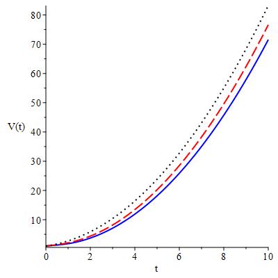
We solve this equation numerically. For simplicity we set $m=1$ and $C_{0}=1$. We consider three case setting $\lambda_{1}=1,\,\lambda=1$ (non-minimal coupling with nonlinear term, blue solid line), $\lambda_{1}=0,\,\lambda=1$ (minimal coupling with nonlinear term, red dash line) and $\lambda_{1}=1,\,\lambda=0$ (non-minimal coupling without nonlinear term, black dot line). In case of nonlinear spinor field we set $n=4$. As the initial condition we set $V(0)=1$ and $\dot{V}(0)=1$. The evolution of the volume scale $V(t)$ is given in Fig. 1

Figure 1: Plot of volume scale $V$ for three different cases with $n=4.$.

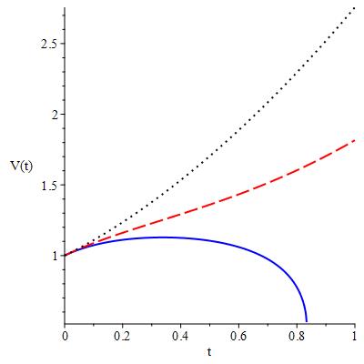
In Fig. 2 we have plotted the evolution of the Universe as in previous case only with $n=5$. In this case for non-minimal coupling with spinor field nonlinearity we see the Universe is closed. After attaining some maximum value the Universe begins to shrink and ends in Big Crunch. It should be noted that in our earlier study with minimal coupling no such results were obtained.

Figure 2: Plot of volume scale $V$ for three different cases with $n=5.$.

As far as FRW case is concerned, we will study this model in some forthcoming paper.

III Discussion and conclusion

Here let us point out a few things. As we have already mentions the spinor field is very sensitive to gravitational one one and the covariant derivative acts on spinor field in a definite way, namely

$$\nabla_{\mu}\psi=\partial_{\mu}\psi-\Gamma_{\mu}\psi,\quad\nabla_{\mu}\bar{\psi}=\partial_{\mu}\bar{\psi}+\bar{\psi}\Gamma_{\mu}.$$

While working with non-minimal coupling we have some construction like $\nabla_{\mu}\nabla_{\nu}S$, where $S=\bar{\psi}\psi$ is a scalar. In this paper we used the property od the spinor field that gives $\nabla_{\mu}S=\partial_{\mu}S$. But what if we use the spinor notation? In that case we have

$$\nabla_{\mu}S = \nabla_{\mu}\left(\bar{\psi}\psi\right)=\left(\nabla_{\mu}\bar{\psi}\right)\psi+\bar{\psi}\left(\nabla_{\mu}\psi\right)$$

$$= \left(\partial_{\mu}\bar{\psi}+\bar{\psi}\Gamma_{\mu}\right)\psi+\bar{\psi}\left(\partial_{\mu}\psi-\Gamma_{\mu}\psi\right)=\left(\partial_{\mu}\bar{\psi}\right)\psi+\bar{\psi}\left(\partial_{\mu}\psi\right)=\partial_{\mu}\left(\bar{\psi}\psi\right)=\partial_{\mu}S.$$

What happens to second derivative?

In one hand

$$\nabla_{\nu}\nabla_{\mu}S=\nabla_{\nu}\partial_{\mu}S=\partial_{\nu}\partial_{\mu}S-\Gamma_{\nu\mu}^{\tau}\partial_{\tau}S.$$ (41)

On the other hand we have

$$\nabla_{\nu}\nabla_{\mu}S = \nabla_{\nu}\partial_{\mu}S=\nabla_{\nu}\left(\partial_{\mu}\bar{\psi}\psi+\bar{\psi}\partial_{\mu}\psi\right)$$ (42)

$$= \left(\nabla_{\nu}\partial_{\mu}\bar{\psi}\right)\psi+\partial_{\mu}\bar{\psi}\nabla_{\nu}\psi+\nabla_{\nu}\bar{\psi}\partial_{\mu}\psi+\bar{\psi}\left(\nabla_{\nu}\partial_{\mu}\psi\right)$$

$$= \left(\partial_{\nu}\partial_{\mu}\bar{\psi}-\Gamma_{\nu\mu}^{\tau}\partial_{\tau}\bar{\psi}\right)\psi+\partial_{\mu}\bar{\psi}\left(\partial_{\nu}\psi-\Gamma_{\nu}\psi\right)$$

$$+ \left(\partial_{\nu}\bar{\psi}+\bar{\psi}\Gamma_{\nu}\right)\partial_{\mu}\psi+\bar{\psi}\left(\partial_{\nu}\partial_{\mu}\psi-\Gamma_{\nu\mu}^{\tau}\partial_{\tau}\psi\right)$$

$$= \partial_{\nu}\partial_{\mu}S-\Gamma_{\nu\mu}^{\tau}\partial_{\tau}S+\left(\bar{\psi}\Gamma_{\nu}\partial_{\mu}\psi-\partial_{\mu}\bar{\psi}\Gamma_{\nu}\psi\right).$$

So in order to get the both (41) and (42) identical, we should have

$$\bar{\psi}\Gamma_{\nu}\partial_{\mu}\psi-\partial_{\mu}\bar{\psi}\Gamma_{\nu}\psi=0.$$ (43)

In our case spinor field depends on $t$ only, whereas $\Gamma_{0}=0$. Taking into account that $\Gamma_{i}=(\dot{a}_{i}/2)\bar{\gamma}^{i}\bar{\gamma}^{0}$, where $i=1,\,2,\,3$ we rewrite the left hand side of (43) as follows

$$\bar{\psi}\Gamma_{\nu}\partial_{\mu}\psi-\partial_{\mu}\bar{\psi}\Gamma_{\nu}\psi=\frac{\dot{a}_{i}}{2}\left(\bar{\psi}\bar{\gamma}^{i}\bar{\gamma}^{0}\dot{\psi}-\dot{\bar{\psi}}\bar{\gamma}^{i}\bar{\gamma}^{0}\psi\right),$$ (44)

which, on account of (12) can be written as

$$\bar{\psi}\Gamma_{\nu}\partial_{\mu}\psi-\partial_{\mu}\bar{\psi}\Gamma_{\nu}\psi=-\dot{a}_{i}\frac{\dot{V}}{V}\bar{\psi}\bar{\gamma}^{i}\psi=-a_{i}\dot{a}_{i}\frac{\dot{V}}{V}\bar{\psi}\gamma^{i}\psi=-a_{i}\dot{a}_{i}\frac{\dot{V}}{V}v^{i}.$$ (45)

As it was shown earlier $v^{\mu}=\bar{\psi}\gamma^{\mu}\psi$ is the vector, constructed spinor fields and in case of BI cosmology it is trivial. As far as LRS-BI or FRW models are concerned, the demand that both (41) and (42) are identical imposes the following restrictions on the components of the spinor field:

$$\psi^{*}_{1}\psi_{4}+\psi^{*}_{2}\psi_{3}+\psi^{*}_{3}\psi_{2}+\psi^{*}_{4}\psi_{1} = 0$$

$$\psi^{*}_{1}\psi_{4}-\psi^{*}_{2}\psi_{3}+\psi^{*}_{3}\psi_{2}-\psi^{*}_{4}\psi_{1} = 0$$

$$\psi^{*}_{1}\psi_{3}-\psi^{*}_{2}\psi_{4}+\psi^{*}_{3}\psi_{1}-\psi^{*}_{4}\psi_{2} = 0$$

Finally we can make the following conclusions. The consideration of non-minimal coupling has no effect on the non-diagonal components of the energy-momentum tensor of the spinor field. As a result, the restrictions on the space-time geometry remain the same as in case of minimal coupling. Nevertheless, the diagonal components of EMT differ. As one sees, while the linear spinor field with non-minimal coupling or non-linear spinor field with minimal coupling in some cases give rise to open universe, the nonlinear spinor field with non-minimal coupling with the same parameters generates model that is close, i.e., after attaining some maximum value begins to decrease and finally shrinks to Big Crunch.

References

• (1) Saha B. Phys. Rev. D 64 123501 (2001).
• (2) Saha B. Phys. Rev. D 74 124030 (2006).
• (3) Saha B. Phys. Part. Nucl. 40 656 (2009).
• (4) Fabbri L. Phys. Rev. D 85 047502 (2012).
• (5) Kremer G.M. and de Souza R.C. Cosmological models with spinor and scalar fields by Noether symmetry approach arXiv:1301.5163v1 [gr-qc] (2013)
• (6) Saha B. Phys. Part. Nucl. 49 146 (2018)
• (7) Carloni et al Non-minimally coupled condensed cosmologies: matching observational data with phase-space arXiv:1811.10300 [Astro-Phys] (2018).