Partition-based Distributionally Robust Optimization via Optimal Transport with Order Cone Constraints

Abstract

In this paper we wish to tackle stochastic programs affected by ambiguity about the probability law that governs their uncertain parameters. Using optimal transport theory, we construct an ambiguity set that exploits the knowledge about the distribution of the uncertain parameters, which is provided by: i) sample data and ii) a-priori information on the order among the probabilities that the true data-generating distribution assigns to some regions of its support set. This type of order is enforced by means of order cone constraints and can encode a wide range of information on the shape of the probability distribution of the uncertain parameters such as information related to monotonicity or multi-modality. We seek decisions that are distributionally robust. In a number of practical cases, the resulting distributionally robust optimization (DRO) problem can be reformulated as a finite convex problem where the a-priori information translates into linear constraints. In addition, our method inherits the finite-sample performance guarantees of the Wasserstein-metric-based DRO approach proposed by Mohajerin Esfahani and Kuhn (2018), while generalizing this and other popular DRO approaches. Finally, we have designed numerical experiments to analyze the performance of our approach with the newsvendor problem and the problem of a strategic firm competing à la Cournot in a market.

1 Introduction

Distributionally robust optimization (DRO) is a powerful modeling framework for optimization under uncertainty that emerges from considering that the probability distribution of the problem’s uncertain parameters is, in itself, also uncertain. This gives rise to the notion of the ambiguity set, that is, a set where the modeler assumes that the true distribution of the problem’s uncertain parameters is contained. The goal of DRO is therefore to find the decision maker’s choice that is optimal against the worst-case probability distribution within the prescribed ambiguity set. Hence, DRO can be seen as a marriage between stochastic programming and robust optimization, working with probability distributions as the former does, while hedging the decision-maker against the worst case as the latter typically aims to do. Since the work of Scarf1958 , many DRO models have been proposed and studied in the technical literature, especially over the last decade, in which DRO has attracted a lot of attention and become very popular in the field of optimization under uncertainty as an alternative to other paradigms. We refer the reader to Keith2021 ; Rahimian2019 for recent surveys on DRO and optimization under uncertainty. Naturally, the construction of the ambiguity set is key to the practical performance of DRO. It is no wonder, therefore, that much effort has been applied to this issue, resulting in several ways to specify and characterize the ambiguity set, namely:

1. Moment-based approach: The ambiguity set is defined as the set of all probability distributions whose moments satisfy certain constraints; see, Delage2010a ; Gao2017a ; Liu2018 ; Liu2019b ; Mehrotra2014 ; Nakao2017a ; Xin2021 ; Zymler2013 , to name a few.

2. Dissimilarity-based approach: The ambiguity set is defined as the set of all probability distributions whose dissimilarity to a prescribed distribution (often referred to as the nominal distribution) is lower than or equal to a given value. Within this category, the choice of the dissimilarity function leads to a wealth of distinct variants:

   1. Optimal-transport-based (OTP) approach: Here, we include the work in Blanchet2021 ; Blanchet2019proc ; Gao2016 ; MohajerinEsfahani2018 ; JMLRShafieezadeh-Abadeh , among many others, all of which use, as the dissimilarity function, the well-known Wasserstein distance, which exhibits some nice statistical convergence properties. Our work is also based on optimal mass transportation and consequently, it falls within this category.

   2. $\phi$-divergences-based approach: This class comprises all those approaches, which use $\phi$-divergences (such as the Kullback-Leibler divergence), for instance, Bayraksan2015 ; Ben-Tal2013 ; Namkoong2016 . We also include in this group the likelihood-based approaches, proposed by Duchi2021 and Wang2016 .

   3. Other measures of dissimilarity: This category includes all other dissimilarity-based procedures for constructing ambiguity sets than those already mentioned, such as those that utilize the family of $\zeta$-structure probability metrics (for example, the total variation metric, the Bounded Lipschitz metric …), see, for example, the work in Rahimian2019mapr and Zhao2015 , and the Prokhorov metric Erdogan2006 .

3. Hypothesis-test-based approach: The ambiguity set is made up of all those probability distributions which, given a data sample, pass a certain hypothesis test with a prescribed confidence level; see, for example, the work in Bertsimas2018a ; Bertsimas2018b ; Chen2019 .

In the work we present here, we focus on ambiguity sets that are formulated by way of an optimal mass transportation problem. In fact, when the cost function in this problem is a metric, we recover the Wasserstein metric, which is indeed a metric for probability measures. According to Blanchet2021 ; Gao2016 ; MohajerinEsfahani2018 , the Wasserstein metric has nice and interesting properties which make it a good choice in DRO, compared to popular alternative choices such as $\phi$-divergences (see Sections 1.1 and 5.1 in Gao2016 , and the Introduction in MohajerinEsfahani2018 for a comparative analysis). Interestingly, the Wassertein distance offers a powerful theoretical framework to establish rates and guarantees of convergence. Furthermore, the conservatism implied by the ambiguity sets, built by means of the Wasserstein metric can be easily controlled, based on those rates.

Other cost functions can be used in the optimal mass transportation problem, but these do not generally result in a metric, which, most likely, makes it much harder to establish rates of convergence and theoretical guarantees.

However, one disadvantage of using the Wasserstein metric is that the worst-case probability distribution may take the form of a Dirac distribution Yue2020 , which is implausible in practice. Ambiguity sets containing unrealistic distributions may result in overly conservative solutions, since protection against these implausible distributions may require a decision that is more expensive than actually needed. Consequently, ambiguity sets that are solely based on a Wasserstein ball may lead to excessively costly solutions. In order to reduce the degree of conservatism, the authors in Gao2017a ; Liu2021scheme ; Wang2018 ; Yao2018 consider ambiguity sets that are formulated using the Wasserstein metric in conjunction with moment constraints. Specifying these constraints, however, requires the estimation of the relevant parameters. Moreover, adding second-order moment information leads to semidefinite programs. In fact, as underlined in Liu2021scheme , although the mixture of moment conditions and the Wasserstein metric allows the decision maker to exclude pathological distributions and results in good out-of-sample performance, only in some special cases, e.g., when the objective function is piecewise linear with respect to the uncertain parameter, can the DRO problem be reformulated as a tractable semidefinite program. For this reason, they propose a method to approximate the solution of DRO problems with ambiguity sets that are based on both moment conditions and the Wasserstein metric.

Our work follows the path of the work in Gao2017a ; Liu2021scheme ; Wang2018 ; Yao2018 : In an attempt to avoid overly conservative solutions, we seek to enrich the specification of Wasserstein ambiguity sets with a-priori information on the true probability distribution of the problem’s uncertain parameters. Nonetheless, unlike the aforementioned approaches, we represent this information in the form of order cone constraints on the probability masses associated with a partition of the sample space. This has the advantage that the inclusion of such a-priori information does not jeopardize the computational tractability of the underlying mathematical program. Our main contributions can be summarized as follows:

1. In real-world decision-making problems, it is common to count on qualitative and expert information conveying some sense of order between the probabilities of occurrence of certain events. For instance, in the multi-item newsvendor problem, the experienced decision maker may state that high demand values for a certain item are more likely to occur than low ones. This can occur, for example, when the true data-generating probability distribution is known or believed to be a mixture of distributions. In this case, determining the number of partitions in our DRO approach would be equivalent to estimating the number of components of the mixture. Indeed, one should use a number of partitions close to the number of distributions in the mixture. The task of inferring that number and the contribution of each component to the mixture is a relevant and well-known problem in statistics, which falls within the so-called realm of finite mixture models (see, Chapter 6 of McLachlan2000 ). In our approach, however, we assume that part of this inference task has already been done and so some of the inference results are available to the decision maker. Our aim is to exploit this type of qualitative information in the construction of the ambiguity set. Most importantly, our DRO approach protects the decision maker against the ambiguity in this inference process. For this purpose, we propose partitioning the support of the random parameter vector and bestow a partial order on (some of) the probability masses of the resulting subregions. This partial order can be described by a graph, which, in turn, can be associated with a convex cone. Consequently, the partial order can be embedded into the formulation of the ambiguity set in the form of conic constraints. The use of these types of cones is well known in the field of statistical inference with order restrictions (see, NEMETH201680 ; Silvapulle2011 ).

2. As shown in the numerical tests, this partial order can be leveraged, among other things, to easily encode multi-modality using linear constraints, as opposed to other approaches based on semidefinite programming (see, for example, the work in Hanasusanto2015 ), with the consequent benefit in terms of computational complexity. The recent papers Chen2019 ; Lam2017 ; Li2019mapr consider ambiguity sets with moment and generalized unimodal constraints. Our approach, however, can practically model a wider range of “shapes” beyond unimodality (see Subsection 2.3 for more details).

3. In addition to the order cone constraints on the probability masses linked to the different subregions of the partitioned sample space, these probability masses can also be treated as random, with their probability distribution belonging to a certain ambiguity set. This way, our modeling framework extends the two popular DRO paradigms proposed by MohajerinEsfahani2018 , and Bayraksan2015 ; Ben-Tal2013 , respectively. Indeed,

   • If we consider one partition only, that is, the entire sample space itself, there is no uncertainty about the associated probability mass (which is, evidently, equal to one) and no partial order can be established. If we now use a distance as the transportation cost function, our DRO framework reduces to that of MohajerinEsfahani2018 .

   • On the contrary, in order to get the DRO framework of Bayraksan2015 ; Ben-Tal2013 , we just need to i) consider a number of partitions such that every partition contains a single data point from the sample, ii) assume that the distribution of their probability masses belongs to a $\phi$-divergence-based ambiguity set and iii) ignore any other information on the true probability distribution of the problem’s uncertain parameters (namely, partial order and ambiguity in the conditional distributions).

   For their part, the authors in Chensim2020 have proposed a different ambiguity set that also covers these two DRO approaches as special cases. However, their ambiguity set does not include the DRO framework we propose, as we note later.

4. Under mild assumptions, we provide a tractable reformulation of our proposed DRO framework and show that it enjoys finite sample and asymptotic consistency guarantees.

5. Finally, we numerically illustrate the benefits in having a-priori information by comparing our DRO framework with the well-known sample average approximation (SAA) solution and the Wasserstein metric-based approach of MohajerinEsfahani2018 . To this end, we consider the single and multi-item newsvendor problems and the problem of a strategic firm competing à la Cournot in a market.

The rest of the paper is organized as follows. Section 2 includes some preliminaries to the optimal transport problem, we formulate the proposed DRO approach and present tractable reformulations. Convergence properties and performance guarantees are theoretically discussed in Section 3. Section 4 provides the results from numerical experiments. Finally, Section 5 concludes the paper.

Notation. We use $\overline{\mathbb{R}}$ to denote the extended real line, and adopt the conventions of its associated arithmetic. Furthermore, $\mathbb{R}_{+}$ denotes the set of non-negative real numbers. We employ lower-case bold face letters to represent vectors and bold face capital letters for matrices. We use $\textrm{diag}(a_{1},\ldots,a_{m})$ for a diagonal matrix of size $m\times m$ whose diagonal elements are equal to $a_{1},\ldots,a_{m}$. Moreover, given a matrix $\mathbf{M}$, its transpose matrix will be written as $\mathbf{M}^{T}$. We define $\mathbf{e}$ as the array with all its components equal to $1$. The inner product of two vectors $\mathbf{u},\mathbf{v}$ (in a certain space) is denoted $\langle\mathbf{u},\mathbf{v}\rangle=\mathbf{u}^{T}\mathbf{v}$. Given any norm $\left\|\cdot\right\|$ in the Euclidean space (of a given dimension $d$), the dual norm is defined as $\left\|\mathbf{u}\right\|_{*}=\sup_{\left\|\mathbf{v}\right\|\leqslant 1}\langle\mathbf{u},\mathbf{v}\rangle$. Given a function $f:\mathbb{R}^{d}\rightarrow\overline{\mathbb{R}}$, we will say that $f$ is a proper function if $f(\mathbf{x})<+\infty$ for at least one $\mathbf{x}$ and $f(\mathbf{x})>-\infty$ for all $\mathbf{x}\in\mathbb{R}^{d}$. Additionally, the convex conjugate function of $f$, $f^{*}$, is defined as $f^{*}(\mathbf{y}):=\sup_{\mathbf{x}\in\mathbb{R}^{d}}\langle\mathbf{y},\mathbf{x}\rangle-f(\mathbf{x})$. It is well known that if $f$ is a proper function, then $f^{*}$ is also a proper function. Given a set $A\subseteq\mathbb{R}^{d}$, we denote its relative interior as $\textrm{relint}(A)$. Similarly, we refer to its interior as $\textrm{int}(A)$. The support function of set $A$, $S_{A}$, is defined as $S_{A}(\mathbf{b}):=\sup_{\mathbf{a}\in A}\langle\mathbf{b},\mathbf{a}\rangle$. The dual cone $\mathcal{C}^{*}$ of a cone $\mathcal{C}$ is given by $\mathcal{C}^{*}:=\{\mathbf{y}\;/\;\langle\mathbf{y},\mathbf{x}\rangle\geqslant 0,\;\forall\mathbf{x}\in\mathcal{C}\}$. We use the symbol $\delta_{\boldsymbol{\xi}}$ to represent the Dirac distribution supported on $\boldsymbol{\xi}$. In addition, we reserve the symbol “$\;\widehat{}\;$” for objects which are dependent on the sample data. The symbols $\mathbb{E}$ and $\mathbb{P}$ denote, respectively, “expectation” and “probability.” Finally, for the rest of the paper we assume that we always have measurability for those objects, whose expected values we consider.

2 Data-driven distributionally robust optimization model

First, we briefly introduce some concepts from the optimal transport problem (also known as the mass transportation problem) that are at the core of the development of our DRO framework.

Intuitively speaking, the optimal transport problem (OTP) centers on the question of how to move masses between two probability distributions in such a way that the transportation cost is minimal. Let $P$ and $Q$ be two probability distributions in a Polish space $S$ such that $P$ is the distribution of mass seen as the origin (i.e. the source) and $Q$ is the distribution of mass seen as the destination (i.e., the sink), and let $c$ be a measurable cost function with $c(x,y)$ representing the cost of moving a unit of mass from location $x$ to location $y$. The OTP can be stated as follows

$$C(P,Q)=\inf_{\Pi}\Big{\{}\int c(x,y)\Pi(dx,dy): \Pi\;\text{is a joint distribution}\;\text{with marginals}\;P\;\text{and }\;Q,\;$$

$$\text{ respectively}\Big{\}}$$

We assume that the cost function $c$ is a non-negative jointly convex lower semicontinuous function such that if $x=y$ , then $c(x,y)=0$. In the remainder of the paper we assume that we have existence and uniqueness of the OTP (see, for example, Theorem 4.1 in Villani2008 ).

For more technical details about the assumptions on the cost function in the OTP, we refer to Villani2008 and Santambrogio2015 . Note that if we choose a distance on $S$ as the cost function (for example, a $p$-norm, with $p\geq 1$, if $S$ is the Euclidean space $\mathbb{R}^{n}$), we get the so-called Wasserstein metric of order 1, which we represent as $\mathcal{W}(P,Q)$ and which is also known as the Kantorovich metric.

It is well known that this probability distance metrizes the weak convergence property. Furthermore, convergence with respect to the Wasserstein metric of order 1 is equivalent to weak convergence plus convergence of the first moment. Wherever the Wasserstein metric of order 1 is used in this paper, we implicitly consider the set of all probability distributions with finite moment of order $1$. Likewise, we refer to the Wasserstein ball of radius $r\geqslant 0$ centered at a certain nominal probability distribution $P_{0}$ , which we denote by $\mathbb{B}_{r}(P_{0})$, as the set of all probability distributions whose Wasserstein metric of order 1 to $P_{0}$ is at most $r$.

2.1 Formulation of the proposed model

Problem (P) below formulates the data-driven distributionally robust optimization (DDRO) framework we propose.

$$\text{(P)}\;\;\inf_{\mathbf{x}\in X}\sup_{Q\in\mathcal{Q}} \ \mathbb{E}_{Q}\left[f(\mathbf{x},\boldsymbol{\xi})\right]$$ (1a)

s.t. $$\mathbb{P}_{Q}\left[\boldsymbol{\xi}\in\Xi_{i}\right]=p_{i},\forall i\in\mathcal{I}$$ (1b)

$$\widetilde{c}(\mathbf{p}-\widehat{\mathbf{p}})\leqslant\rho$$ (1c)

$$\sum_{i\in\mathcal{I}}p_{i}C(Q_{i},\widehat{Q}_{i})\leqslant\varepsilon$$ (1d)

$$Q_{i}\in\mathcal{Q}_{i},\forall i\in\mathcal{I}$$ (1e)

$$\mathbf{p}\in\Theta$$ (1f)

where $X\subseteq\mathbb{R}^{n}$ is the set of feasible decisions, $\boldsymbol{\xi}:\Omega\rightarrow\Xi\subseteq\mathbb{R}^{d}$ is a random vector defined on the measurable space $(\Omega,\mathcal{F})$ with $\sigma$-algebra $\mathcal{F}$, and $\mathcal{Q}$ is the set of all probability distributions over the measurable space $(\Omega,\mathcal{F})$. Moreover, for each $i\in\mathcal{I}$, $Q_{i}$ is the conditional distribution of $Q$ given $\boldsymbol{\xi}\in\Xi_{i}$, that is $Q_{i}=Q(\boldsymbol{\xi}\;/\;\boldsymbol{\xi}\in\Xi_{i})\in\mathcal{Q}_{i}$, with $\mathcal{Q}_{i}$ being the set of all conditional probability distributions of $Q$ given $\boldsymbol{\xi}\in\Xi_{i}$. In this setting, $\mathcal{I}$ is the set of regions $\Xi_{i}$ with pairwise disjoint interiors into which the support set $\Xi$ is partitioned, that is, $\bigcup_{i\in\mathcal{I}}(\Xi_{i})=\Xi$ and $\text{int}(\Xi_{i})\bigcap\text{int}(\Xi_{j})=\emptyset$, $\forall i,j\in\mathcal{I},i\neq j$. Furthermore, we assume that $Q^{*}(\Xi_{i}\cap\Xi_{j})=0,\forall i,j\in\mathcal{I},i\neq j$, where $Q^{*}$ is the true data-generating distribution. This is equivalent to stating that $\{\Xi_{i}\}_{i\in\mathcal{I}}$ constitutes a $Q^{*}$-packing (see a formal definition of this concept in page 50 of Graf2000 ) and will allow us to unequivocally assign samples from $Q^{*}$ to the partitions $\Xi_{i},i\in\mathcal{I}$. Finally, constraint (1c) defines the set of all probability vectors $\mathbf{p}$ that differ from the nominal empirical probability vector $\widehat{\mathbf{p}}$ in at most $\rho$ according to the cost function $\widetilde{c}$. This is a function that quantifies how dissimilar two probability vectors $\mathbf{p}$ and $\mathbf{q}$ are. For this purpose, we require that $\widetilde{c}$ be a non-negative jointly convex lower semicontinuous function such that if $\mathbf{p}=\mathbf{q}$, then $\widetilde{c}(\mathbf{p},\mathbf{q})=0$. As mentioned further on, function $\widetilde{c}$ could, for example, take the form of a norm or a $\phi$-divergence. To ease the notation and the formulation, we use $\boldsymbol{\xi}$ to represent either the random vector $\boldsymbol{\xi}(\omega)$, with $\omega\in\Omega$ or an element of $\mathbb{R}^{d}$. Note that we can consider the probability measure induced by the random vector $\boldsymbol{\xi}$, if we choose the corresponding Borel $\sigma$-algebra $\mathcal{B}$ on $\Xi$. Thus, we can see $\mathcal{Q}$ as a set of probability measures defined over $(\Xi,\mathcal{B})$, so we write $\mathcal{Q}=\mathcal{Q}(\Xi)$. We define the uncertainty set $\mathcal{P}$ for the probability vector $\mathbf{p}\in\mathbb{R}^{|\mathcal{I}|}$, with $|\mathcal{I}|$ being the number of partitions, as the intersection of $\Theta$ and the set defined by constraint (1c). The support set $\Theta$, which includes the order cone constraints on the probability masses $\mathbf{p}$, is given by:

$$\Theta=\{\mathbf{p}\in\mathbb{R}^{|\mathcal{I}|}:\langle\mathbf{e},\mathbf{p}\rangle=1,\mathbf{p}\in\mathbb{R}^{|\mathcal{I}|}_{+},\mathbf{p}\in\mathcal{C}\}$$ (2)

where $\mathcal{C}$ is a proper (convex, closed, full and pointed) cone. Hence, $\Theta$ is a convex compact set.

In problem (P), $\rho$ and $\varepsilon$ are non-negative parameters, to be tuned by the decision maker, which control the size of the ambiguity set defined by equations (1b)–(1f).

We represent this set as $\mathcal{U}_{\rho,\varepsilon}(\widehat{Q})$, where $\widehat{Q}$ is a nominal distribution expressed in terms of $\widehat{\mathbf{p}}$ and $\widehat{Q}_{i}$ as

$$\widehat{Q}=\sum_{i\in\mathcal{I}}{\widehat{p}_{i}\widehat{Q}_{i}}$$ (3)

where

$$\widehat{p}_{i}=\frac{N_{i}}{N+|I^{\prime}|}$$ (4)

and

$$\widehat{Q}_{i}=\frac{1}{N_{i}}\sum_{j=1}^{N_{i}}\delta_{\boldsymbol{\widehat{\xi}}_{j}^{\,\,i}}$$ (5)

Additionally, $I^{\prime}=\{i\in\mathcal{I}\ \textrm{such that partition}\;i\textrm{ does not contain any data from the sample}\}$, $\boldsymbol{\widehat{\xi}}_{j}^{\,\,i}\in\{\boldsymbol{\widehat{\xi}}_{1}^{\,\,i},\ldots,\boldsymbol{\widehat{\xi}}_{N_{i}}^{\,\,i}\}$ and $N_{i}$ is the number of atoms in region $\Xi_{i}$. Here we set $N_{i}=1$ and $\boldsymbol{\widehat{\xi}}^{\,\,i}_{1}:=\arg\sup_{\boldsymbol{\xi}\in\Xi_{i}}f(\mathbf{x},\boldsymbol{\xi})$ for those $i\in I^{\prime}$. Implicitly, we assume that this supremum is attained. We remark that this modeling choice protects the decision maker in those cases where there is a total absence of information on the conditional distributions $Q_{i},i\in I^{\prime}$. Indeed, by introducing the “artificial” data point $\boldsymbol{\widehat{\xi}}^{\,\,i}_{1}:=\arg\sup_{\boldsymbol{\xi}\in\Xi_{i}}f(\mathbf{x},\boldsymbol{\xi})$ in a partition $\Xi_{i}$ with no samples, we are considering the worst-case form that the true conditional distribution $Q_{i}$ could possibly take, that is, a Dirac distribution supported on $\boldsymbol{\widehat{\xi}}^{\,\,i}_{1}$.

Finally, we note that the ambiguity set defined by constraints (1b)–(1f) is unequivocally determined by specifying the partitions $\Xi_{i},i\in\mathcal{I}$, the nominal distribution $\widehat{Q}$, the budgets $\rho$ and $\varepsilon$, and the order cone constraints $\mathbf{p}\in\mathcal{C}$ in (2). In fact, if these constraints are removed and we set $\rho=\varepsilon=0$, then we have $p_{i}=\widehat{p}_{i}$ and $Q_{i}=\widehat{Q}_{i},\forall i$, and therefore, $Q=\widehat{Q}$.

The following theorem shows that problem (P) can be reformulated as a single-level problem.

Theorem 2.1 (Reformulation based on strong duality)

For any non-negative values of parameters $\varepsilon,\rho$, problem (P) is equivalent to the following:

$$\text{(P0)}\;\inf_{\mathbf{x},\lambda,\boldsymbol{\mu},\eta\;\widetilde{\mathbf{p}},\theta,\mathbf{t}} \lambda\rho+\eta+\theta\varepsilon+\lambda\widetilde{c}^{*}_{\mathbf{\widehat{p}}}\left(\frac{\left(\frac{1}{N_{i}}\sum_{j=1}^{N_{i}}t_{i,j}\right)_{i\in\mathcal{I}}+\boldsymbol{\mu}-\eta\mathbf{e}+\widetilde{\mathbf{p}}}{\lambda}\right)$$

s.t. $$t_{i,j}\geqslant\sup_{\boldsymbol{\xi}\in\Xi_{i}}\left[f(\mathbf{x},\boldsymbol{\xi})-\theta c(\boldsymbol{\xi},\widehat{\boldsymbol{\xi}}^{\,i}_{j})\right],\;\forall i\in\mathcal{I},\;j\leqslant N_{i}$$ (6)

$$\mathbf{x}\in X,\lambda\geqslant 0,\boldsymbol{\mu}\in\mathbb{R}^{|\mathcal{I}|}_{+},\eta\in\mathbb{R},\;\widetilde{\mathbf{p}}\in\mathcal{C}^{*},\theta\geqslant 0$$

$$t_{i,j}\in\mathbb{R},\forall i\in\mathcal{I},j\leqslant N_{i}$$

where $\widetilde{c}^{*}_{\mathbf{\widehat{p}}}(\cdot)$ is the convex conjugate function of $\widetilde{c}(\cdot,\mathbf{\widehat{p}})$, with $\mathbf{\widehat{p}}$ fixed, and $\left(\frac{1}{N_{i}}\sum_{j=1}^{N_{i}}t_{i,j}\right)_{i\in\mathcal{I}}$ is the vector with the $|\mathcal{I}|$ components $\frac{1}{N_{i}}\sum_{j=1}^{N_{i}}t_{i,j}$.

Proof

Recall that we have assumed that regions $\Xi_{i}$ are disjoint. Thus, using the law of total probability, we can rewrite problem (P) as follows:

$$\inf_{\mathbf{x}\in X}\sup_{\mathbf{p}\in\mathcal{P}} G(\mathbf{x},\mathbf{p})$$ (7)

where we have considered the subproblem (SP):

$$\text{(SP)}\;G(\mathbf{x},\mathbf{p})= \sup_{Q_{i}\in\mathcal{Q}_{i},\forall i}\sum_{i\in\mathcal{I}}p_{i}\mathbb{E}_{Q_{i}}\left[f(\mathbf{x},\boldsymbol{\xi})\right]$$ (8a)

s.t. $$\sum_{i\in\mathcal{I}}p_{i}C(Q_{i},\widehat{Q}_{i})\leqslant\varepsilon$$ (8b)

The probability distribution $\widehat{Q}_{i}$ is defined as $\widehat{Q}_{i}=\frac{1}{N_{i}}\sum_{j=1}^{N_{i}}\delta_{\boldsymbol{\widehat{\xi}}_{j}^{\,\,i}}$, with $\boldsymbol{\widehat{\xi}}_{j}^{\,\,i}\in\{\boldsymbol{\widehat{\xi}}_{1}^{\,\,i},\ldots,\boldsymbol{\widehat{\xi}}_{N_{i}}^{\,\,i}\}$, and $N_{i}$ being the number of data points in $\Xi_{i}$.

Note that the structure of problem (7) does not fit in the general ambiguity set proposed in Chensim2020 .

Equivalently, we can recast the subproblem (SP) as

(SP) $$=\left\{\begin{array}[]{cl}\displaystyle\sup_{Q_{i}\in\mathcal{Q}_{i},\Pi_{i},\forall i}\sum_{i\in\mathcal{I}}p_{i}&{}\displaystyle\int_{\Xi_{i}}f(\mathbf{x},\boldsymbol{\xi})Q_{i}(d\boldsymbol{\xi})\\ \text{s.t.}&{}\displaystyle\sum_{i\in\mathcal{I}}p_{i}\int_{\Xi_{i}^{2}}c(\boldsymbol{\xi},\boldsymbol{\xi}^{\prime})\Pi_{i}(d\boldsymbol{\xi},d\boldsymbol{\xi}^{\prime})\leqslant\varepsilon\\[4.30554pt] &{}\left\{\begin{array}[]{l}\forall\;i,\;\Pi_{i}\text{ is }\text{ a }\text{ joint }\text{ distribution }\text{ of }\boldsymbol{\xi}\text{ and }\boldsymbol{\xi}^{\prime}\\ \text{ with }\text{ marginals }Q_{i}\text{ and }\widehat{Q}_{i}\text{, }\text{ respectively }\end{array}\right.\end{array}\right.$$ (14)

$$=\left\{\begin{array}[]{cl}\displaystyle\sup_{\widetilde{Q}_{j}^{i},\forall i\in\mathcal{I},j\leqslant N_{i}}&{}\displaystyle\sum_{i\in\mathcal{I}}\frac{p_{i}}{N_{i}}\sum_{j=1}^{N_{i}}\displaystyle\int_{\Xi_{i}}f(\mathbf{x},\boldsymbol{\xi})\widetilde{Q}_{j}^{i}(d\boldsymbol{\xi})\\ \text{s.t.}&{}\displaystyle\sum_{i\in\mathcal{I}}\frac{p_{i}}{N_{i}}\sum_{j=1}^{N_{i}}\int_{\Xi_{i}}c(\boldsymbol{\xi},\widehat{\boldsymbol{\xi}}^{\,i}_{j})\widetilde{Q}_{j}^{i}(d\boldsymbol{\xi})\leqslant\varepsilon\\ &\displaystyle\int_{\Xi_{i}}\widetilde{Q}_{j}^{i}(d\boldsymbol{\xi})=1,\;\forall i\in\mathcal{I},j\leqslant N_{i}\end{array}\right.$$ (18)

where reformulation (18) follows on from the fact that the marginal distribution of $\boldsymbol{\xi}^{\prime}$ is the discrete uniform distribution supported on points $\boldsymbol{\widehat{\xi}}^{\,\,i}_{j}$, $j=1,\ldots,N_{i}$. Thus, $\Pi_{i}$ is completely determined by the conditional distributions $\widetilde{Q}_{j}^{i}=\Pi_{i}(\xi,\xi^{\prime}|\xi^{\prime}=\widehat{\xi}_{j}^{i})$, $\forall i\leqslant N_{i}$, that is, $\Pi_{i}(d\boldsymbol{\xi},d\boldsymbol{\xi}^{\prime})=\frac{1}{N_{i}}\sum_{j=1}^{N_{i}}\delta_{\boldsymbol{\widehat{\xi}}_{j}^{\,i}}(d\boldsymbol{\xi}^{\prime})\widetilde{Q}_{j}^{i}(d\boldsymbol{\xi})$ MohajerinEsfahani2018 .

The mathematical program (18) constitutes a generalized moment problem over the normalized measures $\widetilde{Q}_{j}^{i}$, for which strong duality holds (see, for example, Shapiro2001 ). We can, therefore, dualize the $\varepsilon$-budget constraint on the transport cost, thus obtaining:

$$\displaystyle\inf_{\theta\geqslant 0}\sup_{\widetilde{Q}_{j}^{i},\forall i\in\mathcal{I},j\leqslant N_{i}}\ \theta\varepsilon+\sum_{i\in\mathcal{I}}\frac{p_{i}}{N_{i}}\sum_{j=1}^{N_{i}}\int_{\Xi_{i}}\left[f(\mathbf{x},\boldsymbol{\xi})-\theta c(\boldsymbol{\xi},\widehat{\boldsymbol{\xi}}^{\,i}_{j})\right]\widetilde{Q}_{j}^{i}(d\boldsymbol{\xi})$$ (19)

$$\text{s.t.}\ \int_{\Xi_{i}}\widetilde{Q}_{j}^{i}(d\boldsymbol{\xi})=1,\;\forall i\in\mathcal{I},j\leqslant N_{i}$$ (20)

$$= \inf_{\theta\geqslant 0}\ \theta\varepsilon+\sum_{i\in\mathcal{I}}\frac{p_{i}}{N_{i}}\sum_{j=1}^{N_{i}}\sup_{\widetilde{Q}_{j}^{i}}\int_{\Xi_{i}}\left[f(\mathbf{x},\boldsymbol{\xi})-\theta c(\boldsymbol{\xi},\widehat{\boldsymbol{\xi}}^{\,i}_{j})\right]\widetilde{Q}_{j}^{i}(d\boldsymbol{\xi})$$ (21)

$$\hskip 99.58464pt\text{s.t.}\;\int_{\Xi_{i}}\widetilde{Q}_{j}^{i}(d\boldsymbol{\xi})=1,\;\forall i\in\mathcal{I},j\leqslant N_{i}$$ (22)

$$= \inf_{\theta\geqslant 0}\ \theta\varepsilon+\sum_{i\in\mathcal{I}}\frac{p_{i}}{N_{i}}\sum_{j=1}^{N_{i}}\sup_{\boldsymbol{\xi}\in\Xi_{i}}\left[f(\mathbf{x},\boldsymbol{\xi})-\theta c(\boldsymbol{\xi},\widehat{\boldsymbol{\xi}}^{\,i}_{j})\right]$$ (23)

$$= \inf_{\theta,t_{ij},\forall i\in\mathcal{I},j\leqslant N_{i}}\theta\varepsilon+\sum_{i\in\mathcal{I}}\frac{p_{i}}{N_{i}}\sum_{j=1}^{N_{i}}t_{i,j}$$ (24)

$$\hskip 34.1433pt\text{s.t.}\;t_{i,j}\geqslant\sup_{\boldsymbol{\xi}\in\Xi_{i}}\left[f(\mathbf{x},\boldsymbol{\xi})-\theta c(\boldsymbol{\xi},\widehat{\boldsymbol{\xi}}^{\,i}_{j})\right],\;\forall i\in\mathcal{I},\;j\leqslant N_{i}$$ (25)

$$\hskip 51.21495pt\theta\geqslant 0$$ (26)

where the second equality derives from the fact that we can choose a Dirac distribution supported on $\Xi_{i}$ as $\widetilde{Q}_{j}^{i}$ .

Now, dualizing the $\rho$-budget constraint on the transport cost in the inner supremum of problem (7), we obtain:

$$\inf_{\lambda\geqslant 0} \lambda\rho+\sup_{\mathbf{p}\in\Theta}\left[G(\mathbf{x},\mathbf{p})-\lambda\widetilde{c}(\mathbf{p},\mathbf{\widehat{p}})\right]$$ (27)

Thus,

$$\inf_{\lambda\geqslant 0} \lambda\rho+\sup_{\mathbf{p}\in\Theta}\left[G(\mathbf{x},\mathbf{p})-\lambda\widetilde{c}(\mathbf{p},\mathbf{\widehat{p}})\right]$$ (28)

$$=\inf_{\lambda\geqslant 0} \lambda\rho+\sup_{\mathbf{p}\in\Theta}\left[\inf_{\theta\geqslant 0,(t_{i,j})\;s.t.\eqref{problem_dualized11}}\theta\varepsilon+\sum_{i\in\mathcal{I}}\frac{p_{i}}{N_{i}}\sum_{j=1}^{N_{i}}t_{i,j}-\lambda\widetilde{c}(\mathbf{p},\mathbf{\widehat{p}})\right]$$ (29)

Since function $\theta\varepsilon+\sum_{i\in\mathcal{I}}\frac{p_{i}}{N_{i}}\sum_{j=1}^{N_{i}}t_{i,j}-\lambda\widetilde{c}(\mathbf{p},\mathbf{\widehat{p}})$ is upper semicontinuous and concave in $\mathbf{p}$ on the compact convex set $\Theta$ (recall that $\widetilde{c}$ is nonegative, lower semicontinuous, and convex in $\mathbf{p}$), and linear in $\theta$ and $t_{i,j}$ on the convex set defined by $\theta\geqslant 0$ and (25), we can apply Sion’s min-max theorem (Sion1958 ) and in this way, interchange the innest infimum with the outer supremum. Then, by merging the two infima, we arrive at

$$\inf_{\lambda\geqslant 0,\theta\geqslant 0,(t_{i,j})} \lambda\rho+\theta\varepsilon+\sup_{\mathbf{p}\in\Theta}\left[\sum_{i\in\mathcal{I}}\frac{p_{i}}{N_{i}}\sum_{j=1}^{N_{i}}t_{i,j}-\lambda\widetilde{c}(\mathbf{p},\mathbf{\widehat{p}})\right]$$

$$\text{s.t.}\;t_{i,j}\geqslant\sup_{\boldsymbol{\xi}\in\Xi_{i}}\left[f(\mathbf{x},\boldsymbol{\xi})-\theta_{i}c(\boldsymbol{\xi},\widehat{\boldsymbol{\xi}}^{i}_{j})\right],\;\forall i\in\mathcal{I},\;j\leqslant N_{i}$$

We focus now on the inner supremum,

$$\sup_{\mathbf{p}\in\Theta}\left[\left\langle\mathbf{p},\left(\frac{1}{N_{i}}\sum_{j=1}^{N_{i}}t_{i,j}\right)_{i\in\mathcal{I}}\right\rangle-\lambda\widetilde{c}(\mathbf{p},\mathbf{\widehat{p}})\right]$$ (30)

where we have written $\sum_{i\in\mathcal{I}}\frac{p_{i}}{N_{i}}\sum_{j=1}^{N_{i}}t_{i,j}$ as $\Big{\langle}\mathbf{p},\left(\frac{1}{N_{i}}\sum_{j=1}^{N_{i}}t_{i,j}\right)_{i\in\mathcal{I}}\Big{\rangle}$. This is a concave maximization problem (be aware that $\langle\mathbf{p},\mathbf{H}(\mathbf{x})\rangle-\lambda\widetilde{c}(\mathbf{p},\mathbf{\widehat{p}})$ is a concave function with respect to $\mathbf{p}$ and $\Theta$ is a convex compact set; furthermore, notice that we have $\mathbf{H}(\mathbf{x})=\left(\frac{1}{N_{i}}\sum_{j=1}^{N_{i}}t_{i,j}\right)_{i\in\mathcal{I}}$ in our particular case). Consequently, strong duality holds if a Slater condition is satisfied, that is, if there exists a point $\mathbf{p}^{*}\in\text{relint}(\mathbb{R}^{|\mathcal{I}|}_{+})$ such that $\langle\mathbf{e},\mathbf{p}^{*}\rangle=1$, and $\mathbf{p}^{*}\in\text{int}(\mathcal{C})$ (see, for example, Boyd2004 ). Using a standard duality argument, we dualize the constraints $\mathbf{p}\in\mathbb{R}^{|\mathcal{I}|}_{+}$, $\langle\mathbf{e},\mathbf{p}\rangle=1$ and $\mathbf{p}\in\mathcal{C}$, with associated multipliers $\boldsymbol{\mu}\in\mathbb{R}^{|\mathcal{I}|}_{+}$, $\eta\in\mathbb{R}$ and $\widetilde{\mathbf{p}}\in\mathcal{C}^{*}$, respectively. Thus, we obtain the following problem:

$$\inf_{\eta\in\mathbb{R},\boldsymbol{\mu}\in\mathbb{R}^{|\mathcal{I}|}_{+},\;\widetilde{\mathbf{p}}\in\mathcal{C}^{*}}\sup_{\mathbf{p}}\left\{\left\langle\mathbf{p},\left(\frac{1}{N_{i}}\sum_{j=1}^{N_{i}}t_{i,j}\right)_{i\in\mathcal{I}}\right\rangle-\lambda\widetilde{c}(\mathbf{p},\mathbf{\widehat{p}})+\langle\boldsymbol{\mu},\mathbf{p}\rangle+\eta(1-\langle\mathbf{e},\mathbf{p}\rangle)+\langle\widetilde{\mathbf{p}},\mathbf{p}\rangle\right\}=$$

$$\inf_{\eta\in\mathbb{R},\;\boldsymbol{\mu}\in\mathbb{R}^{|\mathcal{I}|}_{+},\widetilde{\mathbf{p}}\in\mathcal{C}^{*}}\eta+\sup_{\mathbf{p}}\left\{\left\langle\mathbf{p},\left(\frac{1}{N_{i}}\sum_{j=1}^{N_{i}}t_{i,j}\right)_{i\in\mathcal{I}}+\boldsymbol{\mu}-\eta\mathbf{e}+\widetilde{\mathbf{p}}\right\rangle-\lambda\widetilde{c}(\mathbf{p},\mathbf{\widehat{p}})\right\}=$$

$$\inf_{\eta\in\mathbb{R},\;\boldsymbol{\mu}\in\mathbb{R}^{|\mathcal{I}|}_{+},\widetilde{\mathbf{p}}\in\mathcal{C}^{*}}\eta+\lambda\sup_{\mathbf{p}}\left\{\left\langle\mathbf{p},\frac{\left(\frac{1}{N_{i}}\sum_{j=1}^{N_{i}}t_{i,j}\right)_{i\in\mathcal{I}}+\boldsymbol{\mu}-\eta\mathbf{e}+\widetilde{\mathbf{p}}}{\lambda}\right\rangle-\widetilde{c}(\mathbf{p},\mathbf{\widehat{p}})\right\}=$$

$$\inf_{\eta\in\mathbb{R},\;\boldsymbol{\mu}\in\mathbb{R}^{|\mathcal{I}|}_{+},\widetilde{\mathbf{p}}\in\mathcal{C}^{*}}\eta+\lambda\widetilde{c}^{*}_{\mathbf{\widehat{p}}}\left(\frac{\left(\frac{1}{N_{i}}\sum_{j=1}^{N_{i}}t_{i,j}\right)_{i\in\mathcal{I}}+\boldsymbol{\mu}-\eta\mathbf{e}+\widetilde{\mathbf{p}}}{\lambda}\right)$$

where $\widetilde{c}^{*}_{\mathbf{\widehat{p}}}(\cdot)$ is the convex conjugate function of $\widetilde{c}(\cdot,\mathbf{\widehat{p}})$, with $\mathbf{\widehat{p}}$ fixed.

Therefore, problem (7) can be equivalently reformulated as follows:

$$\text{(P0)}\;\inf_{\mathbf{x},\lambda,\boldsymbol{\mu},\eta\;\widetilde{\mathbf{p}},\theta,\mathbf{t}} \lambda\rho+\eta+\theta\varepsilon+\lambda\widetilde{c}^{*}_{\mathbf{\widehat{p}}}\left(\frac{\left(\frac{1}{N_{i}}\sum_{j=1}^{N_{i}}t_{i,j}\right)_{i\in\mathcal{I}}+\boldsymbol{\mu}-\eta\mathbf{e}+\widetilde{\mathbf{p}}}{\lambda}\right)$$

s.t. $$t_{i,j}\geqslant\sup_{\boldsymbol{\xi}\in\Xi_{i}}\left[f(\mathbf{x},\boldsymbol{\xi})-\theta c(\boldsymbol{\xi},\widehat{\boldsymbol{\xi}}^{\,i}_{j})\right],\;\forall i\in\mathcal{I},\;j\leqslant N_{i}$$

$$\mathbf{x}\in X,\lambda\geqslant 0,\boldsymbol{\mu}\in\mathbb{R}^{|\mathcal{I}|}_{+},\eta\in\mathbb{R},\;\widetilde{\mathbf{p}}\in\mathcal{C}^{*},\theta\geqslant 0$$

$$t_{i,j}\in\mathbb{R},\forall i\in\mathcal{I},j\leqslant N_{i}$$

Moreover, in the case that the cost function $\widetilde{c}(\cdot,\cdot)$ is given by a norm, we have $\widetilde{c}_{\mathbf{\widehat{p}}}(\mathbf{p})=\left\|\mathbf{p}-\widehat{\mathbf{p}}\right\|$. The next corollary deals with this particular case.

Corollary 1

If the cost functions $c(\cdot,\cdot)$ and $\widetilde{c}(\cdot,\cdot)$ are given by norms, then for any non-negative values of parameters $\varepsilon,\rho$, the problem (P) is equivalent to the following problem

$$\text{(P1)}\;\;\inf_{\mathbf{x},\lambda,\boldsymbol{\mu},\eta\;\widetilde{\mathbf{p}},\theta,\mathbf{t}} \lambda\rho+\eta+\theta\varepsilon+\sum_{i\in\mathcal{I}}\widehat{p}_{i}\left(\frac{1}{N_{i}}\sum_{j=1}^{N_{i}}t_{i,j}+\mu_{i}-\eta+\widetilde{p}_{i}\right)$$

s.t. $$t_{i,j}\geqslant\sup_{\boldsymbol{\xi}\in\Xi_{i}}\left[f(\mathbf{x},\boldsymbol{\xi})-\theta\left\|\boldsymbol{\xi}-\widehat{\boldsymbol{\xi}}^{\,i}_{j}\right\|\right],\forall i\in\mathcal{I},\forall j\leqslant N_{i}$$ (31)

$$\left\|\left(\frac{1}{N_{i}}\sum_{j=1}^{N_{i}}t_{i,j}+\mu_{i}-\eta+\widetilde{p}_{i}\right)_{i\in\mathcal{I}}\right\|_{*}\leqslant\lambda$$

$$\mathbf{x}\in X,\lambda\geqslant 0,\boldsymbol{\mu}\in\mathbb{R}^{|\mathcal{I}|}_{+},\eta\in\mathbb{R},\;\widetilde{\mathbf{p}}\in\mathcal{C}^{*},\theta\geqslant 0$$

$$t_{i,j}\in\mathbb{R},\forall i\in\mathcal{I},\forall j\leqslant N_{i}$$

Proof

We use the following Lemma to put problem (P0) in a better shape.

Lemma 1

Let $\widetilde{c}_{\mathbf{\widehat{p}}}(\mathbf{p})=\left\|\mathbf{p}-\widehat{\mathbf{p}}\right\|$, where $\widehat{\mathbf{p}}\in\mathbb{R}^{|\mathcal{I}|}$ is a fixed vector and $\|\cdot\|$ a norm in $\mathbb{R}^{|\mathcal{I}|}$. Then, it holds that the convex conjugate function of $\widetilde{c}_{\mathbf{\widehat{p}}}(\mathbf{p})$ is as follows

$$\widetilde{c}^{*}_{\mathbf{\widehat{p}}}(\mathbf{s})=\left\{\begin{array}[]{lr}\sum_{i\in\mathcal{I}}\widehat{p}_{i}s_{i}&\text{if}\quad\left\|\mathbf{s}\right\|_{*}\leqslant 1\\ \infty&\text{if}\quad\left\|\mathbf{s}\right\|_{*}>1\end{array}\right.$$

Proof

The claim of the Lemma follows from Proposition 5.1.4. (vii) and Example 5.1.2 (b) of Lucchetti2006 .∎

Therefore, problem (P0) reduces to

$$\text{(P1)}\;\;\inf_{\mathbf{x},\lambda,\boldsymbol{\mu},\eta\;\widetilde{\mathbf{p}},\theta,\mathbf{t}} \lambda\rho+\eta+\theta\varepsilon+\sum_{i\in\mathcal{I}}\widehat{p}_{i}\left(\frac{1}{N_{i}}\sum_{j=1}^{N_{i}}t_{i,j}+\mu_{i}-\eta+\widetilde{p}_{i}\right)$$

s.t. $$t_{i,j}\geqslant\sup_{\boldsymbol{\xi}\in\Xi_{i}}\left[f(\mathbf{x},\boldsymbol{\xi})-\theta\left\|\boldsymbol{\xi}-\widehat{\boldsymbol{\xi}}^{\,i}_{j}\right\|\right],\forall i\in\mathcal{I},\forall j\leqslant N_{i}$$

$$\left\|\left(\frac{1}{N_{i}}\sum_{j=1}^{N_{i}}t_{i,j}+\mu_{i}-\eta+\widetilde{p}_{i}\right)_{i\in\mathcal{I}}\right\|_{*}\leqslant\lambda$$

$$\mathbf{x}\in X,\lambda\geqslant 0,\boldsymbol{\mu}\in\mathbb{R}^{|\mathcal{I}|}_{+},\eta\in\mathbb{R},\;\widetilde{\mathbf{p}}\in\mathcal{C}^{*},\theta\geqslant 0$$

$$t_{i,j}\in\mathbb{R},\forall i\in\mathcal{I},\forall j\leqslant N_{i}$$

∎

Remarks. Our data-driven DRO framework (P) can be easily understood as a generalization of other popular DRO approaches. To see this, first we need to remove the order cone constraints on the probabilities associated with each subregion into which the support $\Xi$ has been partitioned, that is, the condition $\mathbf{p}\in\mathcal{C}$, and then proceed as indicated below:

1. If we set $\varepsilon=0$, $|\mathcal{I}|=N$, with every partition containing a single and different data point from the sample, and use a $\phi$-divergence to build the cost function, i.e., $\widetilde{c}_{\mathbf{\widehat{p}}}(\mathbf{p})=\sum_{i\in\mathcal{I}}\widehat{p}_{i}\phi\left(\frac{p_{i}}{\widehat{p}_{i}}\right)$ and hence, $c^{*}_{\mathbf{\widehat{p}}}(\mathbf{s})=\sum_{i\in\mathcal{I}}\widehat{p}_{i}\phi^{*}(s_{i})$, then our data-driven DRO approach boils down to that of Ben-Tal2013 and Bayraksan2015 .

2. On the contrary, if we set $|\mathcal{I}|=1$, $c$ is given by a norm and take $\widetilde{c}_{\mathbf{\widehat{p}}}(\mathbf{p})=\left\|\mathbf{p}-\widehat{\mathbf{p}}\right\|$ (hence $\widetilde{c}^{*}_{\mathbf{\widehat{p}}}(\mathbf{s})=\sum_{i\in\mathcal{I}}\widehat{p}_{i}s_{i}$ if $\left\|\mathbf{s}\right\|_{*}\leqslant 1$), we get the model of MohajerinEsfahani2018 .

Finally, we remark that constraint (6) for each $i\in I^{\prime}$ is equivalent (under the assumptions we make on the transportation cost function) to $t_{i,1}\geqslant\sup_{\xi\in\Xi_{i}}f(x,\xi)$.

2.2 Tractable reformulations

In this section we provide nice reformulations of our DRO model (P) under mild assumptions. For this purpose, we make use of the theoretical foundations laid out in MohajerinEsfahani2018 . Likewise, some extensions to our model, such as the extension to two-stage stochastic programming problems, are omitted here for brevity and because they can be easily derived in a similar way as found in MohajerinEsfahani2018 for the data-driven DRO approach they develop.

We start our theoretical development with the following assumption.

Assumption 1

We consider that $\Xi_{i}$, for each $i\in\mathcal{I}$, is a closed convex set, and that $f(\mathbf{x},\boldsymbol{\xi}):=$ $\max_{k\leqslant K}g_{k}(\mathbf{x},\boldsymbol{\xi})$, with $g_{k}$, for each $k\leqslant K$, being a proper, concave and upper semicontinuous function with respect to $\boldsymbol{\xi}$ (for any fixed value of $\mathbf{x}\in X$) and not identically $\infty$ on $\Xi_{i}$.

Theorem 2.2 below provides a tractable reformulation of problem (P1) as a finite convex problem. For ease of notation, we suppress the dependence on the variable $\mathbf{x}$ (bearing in mind that this dependence occurs through functions $g_{k}$, $k\leqslant K$).

Theorem 2.2

If Assumption 1 holds and if we choose a norm (in $\mathbb{R}^{d}$) as the transportation cost function $c$, then for any values of $\rho$ and $\varepsilon$, problem (P1) is equivalent to the following finite convex problem:

$$\text{(P1')}\;\;\inf_{\mathbf{x},\lambda,\eta,\boldsymbol{\mu},\;\widetilde{\mathbf{p}},\mathbf{z}_{ijk},\mathbf{v}_{ijk},\theta,\mathbf{t}} \lambda\rho+\eta+\theta\varepsilon+\sum_{i\in\mathcal{I}}\widehat{p}_{i}\left(\frac{1}{N_{i}}\sum_{j=1}^{N_{i}}t_{i,j}+\mu_{i}-\eta+\widetilde{p}_{i}\right)$$

s.t. $$t_{i,j}\geqslant[-g_{k}]^{*}(\mathbf{z}_{ijk}-\mathbf{v}_{ijk})+S_{\Xi_{i}}(\mathbf{v}_{ijk})-\langle\mathbf{z}_{ijk},\widehat{\boldsymbol{\xi}}^{\,i}_{j}\rangle$$

$$\forall i\in\mathcal{I},\forall j\leqslant N_{i},\forall k\leqslant K$$

$$\left\|\mathbf{z}_{ijk}\right\|_{*}\leqslant\theta,\forall i\in\mathcal{I},\forall j\leqslant N_{i},\forall k\leqslant K$$

$$\left\|\left(\frac{1}{N_{i}}\sum_{j=1}^{N_{i}}t_{i,j}+\mu_{i}-\eta+\widetilde{p}_{i}\right)_{i\in\mathcal{I}}\right\|_{*}\leqslant\lambda$$

$$\mathbf{x}\in X,\lambda\geqslant 0,\theta\geqslant 0,\eta\in\mathbb{R},\boldsymbol{\mu}\in\mathbb{R}_{+}^{|\mathcal{I}|},\;\widetilde{\mathbf{p}}\in\mathcal{C}^{*},$$

$$\mathbf{z}_{ijk},\mathbf{v}_{ijk}\in\mathbb{R}^{d},\forall i\in\mathcal{I},\forall j\leqslant N_{i},\forall k\leqslant K$$

$$t_{i,j}\in\mathbb{R},\forall i\in\mathcal{I},\forall j\leqslant N_{i}$$

where $[-g_{k}]^{*}(\mathbf{z}_{ijk}-\mathbf{v}_{ijk})$ is the conjugate function of $-g_{k}$ evaluated at $\mathbf{z}_{ijk}-\mathbf{v}_{ijk}$ and $S_{\Xi_{i}}$ is the support function of $\Xi_{i}$.

Proof

In essence, the complexity of problem (P1) depends on our ability to reformulate the supremum in constraint (31) in a tractable manner. This is possible under Asummption 1, following similar steps to those in the proof of Theorem 4.2 in MohajerinEsfahani2018 , to which we refer. ∎

We note that Asummption 1 covers the particular case where functions $g_{k}$, $k\leqslant K$, are affine and, as a result, $f$ is convex piecewise linear. The single-item newsvendor problem, which we illustrate in the first part of Section 4, constitutes a popular example of this case.

2.2.1 Separable objective function

Now we extend the results presented above to a class of objective functions which are additively separable with respect to the dimension $d$. We assume here that $\boldsymbol{\xi}=(\boldsymbol{\xi}_{1},\ldots,\boldsymbol{\xi}_{d})$, where $\boldsymbol{\xi}_{l}\in\mathbb{R}^{p}$, for each $l=1,\ldots,d$. Furthermore, we consider the separable norm $\left\|\boldsymbol{\xi}\right\|_{d}:=\sum_{l=1}^{d}\left\|\boldsymbol{\xi}_{l}\right\|$ associated with the base norm $\left\|\cdot\right\|$ (on $\mathbb{R}^{p}$). Finally, we assume that the function $f$ is given as follows:

$$f(\mathbf{x},\boldsymbol{\xi})=\sum_{l=1}^{d}\max_{k\leqslant K}g_{lk}(\mathbf{x},\boldsymbol{\xi}_{l})$$ (32)

In this case, the complexity of the resulting DRO problem is linear with respect to the number $N$ of samples. The multi-item newsvendor problem, which we illustrate in the second half of Section 4, constitutes a popular example of this case.

Theorem 2.3

If $f(\mathbf{x},\boldsymbol{\xi})=\sum_{l=1}^{d}\max_{k\leqslant K}g_{lk}(\mathbf{x},\boldsymbol{\xi}_{l})$, $\{g_{lk}\}_{k\leqslant K}$ satisfy Assumption 1 for all $l\leqslant d$, and $\Xi_{i}$, for each $i\in\mathcal{I}$, is given by the Cartesian product of closed convex sets (that is, $\Xi_{i}:=\prod_{l=1}^{d}D_{l}^{i}$, with $D_{l}^{i}$ a closed convex set), and if we choose the norm $\left\|\cdot\right\|_{d}$ as the transportation cost function $c$, then for any values of $\rho$ and $\varepsilon$, problem (P) is equivalent to the following finite convex problem:

$$\text{(P2)}\;\;\inf_{\mathbf{x},\lambda,\eta,\boldsymbol{\mu},\;\widetilde{\mathbf{p}},\mathbf{z}_{ijkl},\mathbf{v}_{ijkl},\theta,\boldsymbol{\omega}} \lambda\rho+\eta+\theta\varepsilon+\sum_{i\in\mathcal{I}}\widehat{p}_{i}\left(\frac{1}{N_{i}}\sum_{j=1}^{N_{i}}\sum_{l=1}^{d}\omega_{ijl}+\mu_{i}-\eta+\widetilde{p}_{i}\right)$$ (33)

s.t. $$\omega_{ijl}\geqslant[-g_{lk}]^{*}(\mathbf{z}_{ijkl}-\mathbf{v}_{ijkl})+S_{D_{l}^{i}}(\mathbf{v}_{ijkl})-\langle\mathbf{z}_{ijkl},\widehat{\boldsymbol{\xi}}^{\,i}_{jl}\rangle,$$ (34)

$$\forall i\in\mathcal{I},\forall j\leqslant N_{i},\forall k\leqslant K,\forall l\leqslant d$$

$$\left\|\mathbf{z}_{ijkl}\right\|_{*}\leqslant\theta,\forall i\in\mathcal{I},\forall j\leqslant N_{i},\forall k\leqslant K,\forall l\leqslant d$$ (35)

$$\left\|\left(\frac{1}{N_{i}}\sum_{j=1}^{N_{i}}\sum_{l=1}^{d}\omega_{ijl}+\mu_{i}-\eta+\widetilde{p}_{i}\right)\right\|_{*}\leqslant\lambda$$ (36)

$$\mathbf{x}\in X,\lambda\geqslant 0,\theta\geqslant 0,\eta\in\mathbb{R},\boldsymbol{\mu}\in\mathbb{R}_{+}^{|\mathcal{I}|},\;\widetilde{\mathbf{p}}\in\mathcal{C}^{*},$$ (37)

$$\omega_{ijl}\in\mathbb{R},\forall i\in\mathcal{I},\forall j\leqslant N_{i},\forall l\leqslant d$$ (38)

$$\mathbf{z}_{ijkl},\mathbf{v}_{ijkl}\in\mathbb{R}^{p},\forall i\in\mathcal{I},\forall j\leqslant N_{i},\forall k\leqslant K,\forall l\leqslant d$$ (39)

Proof

The proof runs in a similar way to that of Theorem 6.1 in MohajerinEsfahani2018 . ∎

Remarks. If the transportation cost function $c$ is not a norm, there are still some cases where the constraint (6) can be reformulated in a tractable way. In general, equation (6) can be seen as the robust counterpart of a constraint affected by the random parameter vector $\boldsymbol{\xi}$, with $\Xi_{i}$ playing the role of the so-called uncertainty set. In our case, the tractability of (6) depends on the nature of each set $\Xi_{i}$ and each function $\alpha_{ij}(\boldsymbol{\xi}):=f(\mathbf{x},\boldsymbol{\xi})-\theta c(\boldsymbol{\xi},\widehat{\boldsymbol{\xi}}^{\,i}_{j})$. Indeed, suppose that every $\Xi_{i}$ is a closed convex set, then:

• If the function $f$ is concave in $\boldsymbol{\xi}$, so is each function $\alpha_{ij}(\boldsymbol{\xi})$ (recall that the transportation cost function $c$ is assumed to be convex and that $\theta$ is non-negative). As Roos2018a points out, this is a tractable instance and tractable reformulations of constraint (6) can be obtained using Fenchel duality following the guidelines in Ben-Tal2015 .

• In contrast, the case in which some $\alpha_{ij}(\boldsymbol{\xi})$ are convex is much more challenging and may call for approximation methods such as the one proposed by Roos2018a .

In any case, we need to compute convex conjugate functions, which is, in itself, a complicated problem in general. For assistance in this regard, one may resort to symbolic computation in order to get closed formulas for convex conjugate functions (see, for example, Borwein2009 ).

2.3 Order cone constraints

To account for a-priori knowledge about the probability distribution of the random parameter vector $\boldsymbol{\xi}$ (for example, the decision maker may have some information about the shape of this distribution), we propose to convey this knowledge using order constraints on the probability masses $p_{i}$ associated with each subregion $\Xi_{i}$ into which the support $\Xi$ of $\boldsymbol{\xi}$ is partitioned. These order constraints are based on order cones, which, in turn, can be represented in the form of graphs.

We can build order cones from graphs that allow for the comparison of all probabilities $p_{i}$. In that case, we say that the graph, and the associated cone, establish a total order. If, on the contrary, the graph only allows some of those probabilities to be compared, we talk about partial order. For more details about order cones we refer the reader to NEMETH201680 .

Below, we present some common choices of order cones.

• Simple order cone (monotonicity):

  $$\mathcal{C}=\{p\in\mathbb{R}^{|\mathcal{I}|}:p_{1}\geqslant\ldots\geqslant p_{|\mathcal{I}|}\}$$

• Tree order cone:

  $$\mathcal{C}=\{p\in\mathbb{R}^{|\mathcal{I}|}:p_{i}\geqslant p_{|\mathcal{I}|},\;i=1,\ldots,|\mathcal{I}|-1\}$$

• Star-shaped cone (decrease on average):

  $$\mathcal{C}=\Big{\{}p\in\mathbb{R}^{|\mathcal{I}|}:p_{1}\geqslant\frac{p_{1}+p_{2}}{2}\geqslant\ldots\geqslant\frac{p_{1}+\ldots+p_{|\mathcal{I}|}}{|\mathcal{I}|}\Big{\}}$$

• Umbrella cone (unimodality):

  $$\mathcal{C}=\{p\in\mathbb{R}^{|\mathcal{I}|}:p_{1}\leqslant p_{2}\leqslant\ldots\leqslant p_{m}\geqslant p_{m+1}\geqslant\ldots\geqslant p_{|\mathcal{I}|}\}$$

An order cone is a polyhedral convex cone and as such, can be algebraically expressed in the form $\mathcal{C}=\{\mathbf{p}\in\mathbb{R}^{|\mathcal{I}|}:\mathbf{A}\mathbf{p}\geqslant 0\}$, with $\mathbf{A}$ being a matrix of appropriate dimensions. Its dual $\mathcal{C}^{*}$ can, therefore, be easily computed as $\mathcal{C}^{*}=\{\mathbf{\widetilde{p}}=\mathbf{A}^{T}\boldsymbol{\nu}:\boldsymbol{\nu}\geqslant\mathbf{0}\}$ (see, for instance, Corollary 3.12.9 in Silvapulle2011 ). Notwithstanding, our DRO approach can be equally applied under other types of support sets, as long as the problem (30) admits a strong dual (we refer the interested reader to Ben-Tal2013 for a list of types of support sets under which strong duality holds).

As compared to other approaches available in the technical literature, order cones provide a straightforward way of encoding modality information in the ambiguity set of the DRO problem. For instance, Hanasusanto2015 indirectly introduces multi-modality information by imposing first and second moment conditions on the different ambiguous components of a mixture with known weights. Their approach, however, results in a semidefinite program. Unlike Hanasusanto2015 , the authors in Li2019mapr explicitly incorporate modality information into their ambiguity set through moment and generalized unimodal constraints. Nonetheless, they still need to solve a semidefinite program and their DRO approach overlooks the data-driven nature of those constraints. In Chen2019 , they construct an ambiguity set made up of those absolutely continuous probability distributions whose density function is bounded by some bands with a certain confidence level. Their approach can be used to impose monotonicity or unimodality of the probability distributions, but can only be applied to the univariate case.

Beyond modality, the order cone constraints on the partition probabilities that characterize our DRO approach equip the decision maker with a versatile and intuitive framework to exploit information on the shape of the ambiguous probability distribution. For example, as we do in the numerical experiments in Section 4, we can construct an order cone that constrains the ratios among the partition probabilities, which can be seen as a discrete approximation of encoding “derivative” information on the ambiguous probability distribution (if this admits a density function). Likewise, other order cones could be used to bestow some sense of “convexity” on this distribution.

3 On convergence and out-of-sample performance guarantees

In this section, we show that our DRO approach (P) naturally inherits the convergence and performance guarantees of that introduced in MohajerinEsfahani2018 . For this purpose, we first need to recall some terminology and concepts from this paper to which we will resort later on. Throughout this section, we denote the training data sample (that is, the sample path sequence) as $\widehat{\Xi}_{N}:=\{\widehat{\boldsymbol{\xi}^{i}}\}_{i=1}^{N}\subseteq\Xi$. Following MohajerinEsfahani2018 , $\widehat{\Xi}_{N}$ can be seen as a random vector governed by the probability distribution $\mathbb{P}^{N}:=Q^{*}\times\cdots\times Q^{*}$ ($N$ times) supported on $\Xi^{N}$ (with the respective product $\sigma$-algebra).

In the remainder of this paper, we will denote the optimization problem associated with problem $(P)$ under the true probability distribution $Q^{*}$ as (${\rm P}^{*}$) (that is, the problem defined as $J^{*}:=\inf_{\mathbf{x}\in X}\mathbb{E}_{Q^{*}}[f(\mathbf{x},\boldsymbol{\xi})]$). We then say that a data-driven solution for problem (${\rm P}^{*}$) is a feasible solution $\widehat{\mathbf{x}}_{N}\in X$ which is constructed from the sample data. Furthermore, the out-of-sample performance of a data-driven solution $\widehat{\mathbf{x}}_{N}$ is defined as $\mathbb{E}_{Q^{*}}[f(\widehat{\mathbf{x}}_{N},\boldsymbol{\xi})]$.

In line with MohajerinEsfahani2018 , given a data-driven solution $\widehat{\mathbf{x}}_{N}$, a finite sample guarantee is a relation in the form

$$\mathbb{P}^{N}\Big{[}\widehat{\Xi}_{N}\;:\;\mathbb{E}_{Q^{*}}[f(\widehat{\mathbf{x}}_{N},\boldsymbol{\xi})]\leqslant\widehat{J}_{N}\Big{]}\geqslant 1-\beta$$ (40)

where $\widehat{J}_{N}$ is a certificate for the out-of-sample performance of $\widehat{\mathbf{x}}_{N}$ (i.e., an upper bound that is generally contingent on the training dataset), $\beta\in(0,1)$ is a significance parameter with respect to the distribution $\mathbb{P}^{N}$, on which both $\widehat{\mathbf{x}}_{N}$ and $\widehat{J}_{N}$ depend. Moreover, we refer to the probability on the left-hand side of (40) as the reliability of $(\widehat{\mathbf{x}}_{N},\widehat{J}_{N})$.

Ideally, we strive to develop a method capable of identifying a highly reliable data-driven solution with a certificate as low as possible.

The data-driven DRO approach that we propose in this paper to address problem (${\rm P}^{*}$) accounts for the uncertainty about the true data-generating distribution $Q^{*}$, while taking advantage of some a-priori order information that the decision maker may have on some probabilities induced by $Q^{*}$ over a partition of the support set $\Xi$. Below, we claim that the pair ($\widehat{\mathbf{x}}_{N}$, $\widehat{J}_{N}$) provided by our distributionally robust optimization problem (P) features performance guarantees in line with those discussed in MohajerinEsfahani2018 . More specifically, for a suitable choice of the ambiguity set, the optimal value $\widehat{J}_{N}$ of problem (P) constitutes a certificate of the type (40) providing a confidence level $1-\beta$ on the out-of-sample performance of the data-driven solution $\widehat{\mathbf{x}}_{N}$. This can be formally stated under some assumptions about the underlying true conditional probability distributions.

To this end, we first provide probabilistic guarantees on the partition probabilities $p_{i}$, $\forall i\leqslant|\mathcal{I}|$. In this vein, note that the empirical probability $\widehat{p}_{i}$, defined as in Equation (4), can be modeled as a binomial distribution with success probability $p_{i}^{*}$, divided by the total number of trials. Consequently, by the Strong Law of Large Numbers (SLLN), $\widehat{p}_{i}$ converges to $p_{i}^{*}$ almost surely.

Now suppose that we choose a $\phi$-divergence as $\widetilde{c}$, where $\phi$ is a twice continuously differentiable function around 1 with $\phi^{\prime\prime}(1)>0$. Then, take $\beta_{p}>0$. If we choose as $\rho$ the value

$$\rho(\beta_{p}):=(\phi^{\prime\prime}(1)/(2N))\chi^{2}_{|\mathcal{I}|-1,1-\beta_{p}}$$ (41)

we get a confidence set of level $1-\beta_{p}$ on the true partition probabilities $\mathbf{p}^{*}$ (see Ben-Tal2013 and Bayraksan2015 ).

If, alternatively, we choose the total variation distance as $\widetilde{c}$, we can use Equation (19) in Guo2019 to take $\rho$ as

$$\rho(\beta_{p}):=(|\mathcal{I}|/\sqrt{N})(2+\sqrt{2\log(|\mathcal{I}|/\beta_{p})})$$ (42)

and obtain a confidence set of level $1-\beta_{p}$ on $\mathbf{p}^{*}$.

Next we establish a concentration tail inequality of the probability weighted Wasserstein metric of order 1 between each conditional distribution and its respective true conditional distribution. For this purpose, we first need to make the following assumption:

Assumption 2 (Light-tailed Conditional Distributions)

For each $i\in\mathcal{I}$, there exist $a_{i},\gamma_{i}\in\mathbb{R}$, with $a_{i}>1$ and $\gamma_{i}>0$ such that

$$\mathbb{E}_{Q_{i}^{*}}\big{[}\exp(\gamma_{i}\|\boldsymbol{\xi}\|^{a_{i}})\big{]}=\int_{\Xi_{i}}\exp(\gamma_{i}\|\boldsymbol{\xi}\|^{a_{i}})\,Q_{i}^{*}(\mathrm{d}\boldsymbol{\xi})<\infty.$$ (43)

The following theorem provides a tail concentration inequality for the weighted sum of the Wasserstein metrics of order 1 between the true and empirical conditional distributions.

Theorem 3.1 (Concentration Inequality for the Conditional Distributions )

If Assumption 2 holds, for each $i\in\mathcal{I}$, given $\beta_{i}\in(0,1]$ we have that $\forall N_{i}\geqslant 1$, $\dim(\boldsymbol{\xi})\neq 2$ and for all $\varepsilon>\sum_{i\in\mathcal{I}}p_{i}\varepsilon_{N_{i}}(\beta_{i})$, for any values $p_{i},i\in\mathcal{I}$ such that $p_{i}\geqslant 0$ and $\sum_{i\in\mathcal{I}}p_{i}=1$, the following holds

$$\mathbb{P}\left[\sum_{i\in\mathcal{I}}p_{i}\mathcal{W}(Q_{i}^{*},\widehat{Q}_{i}\big{)}\leqslant\varepsilon\right]\geqslant 1-\sum_{i\in\mathcal{I}}\beta_{i}$$ (44)

where

$$\varepsilon_{N_{i}}(\beta_{i}){:=}\left\{\begin{array}[]{ll}\Big{(}{\log(B_{i}\beta_{i}^{-1})\over C_{i}N_{i}}\Big{)}^{1/\max\{\dim(\boldsymbol{\xi}),2\}}&{}\quad\text{if }N_{i}\geq{\log(B_{i}\beta_{i}^{-1})\over C_{i}},\\ \Big{(}{\log(B_{i}\beta_{i}^{-1})\over C_{i}N_{i}}\Big{)}^{1/a_{i}}&{}\quad\text{if }N_{i}<{\log(B_{i}\beta_{i}^{-1})\over C_{i}}.\end{array}\right.$$ (47)

Proof. Given Assumption 3, for all $i\in\mathcal{I}$, we deduce from Theorem 2 in Fournier2015 that

$$\mathbb{P}\left[\mathcal{W}(Q_{i}^{*},\widehat{Q}_{i})\leqslant\varepsilon_{N_{i}}(\beta_{i})\right]\geqslant 1-\beta_{i}.$$

Thus, we have that

$$\mathbb{P}\left[\sum_{i\in\mathcal{I}}p_{i}\mathcal{W}(Q_{i}^{*},\widehat{Q}_{i})\leqslant\sum_{i\in\mathcal{I}}p_{i}\varepsilon_{N_{i}}(\beta_{i})\right]\geqslant \;\mathbb{P}\left[\bigcap_{i\in\mathcal{I}}\left(p_{i}\mathcal{W}(Q_{i}^{*},\widehat{Q}_{i})\leqslant p_{i}\varepsilon_{N_{i}}(\beta_{i})\right)\right]$$ (48)

$$= 1-\mathbb{P}\left[\bigcup_{i\in\mathcal{I}}\left(p_{i}\mathcal{W}(Q_{i}^{*},\widehat{Q}_{i})>p_{i}\varepsilon_{N_{i}}(\beta_{i})\right)\right]$$ (49)

$$\geqslant 1-\sum_{i\in\mathcal{I}}\mathbb{P}\left[p_{i}\mathcal{W}(Q_{i}^{*},\widehat{Q}_{i})>p_{i}\varepsilon_{N_{i}}(\beta_{i})\right]$$ (50)

$$\geqslant 1-\sum_{i\in\mathcal{I}}\beta_{i}$$ (51)

Theorem 3.1 sets the probabilistic bound $\sum_{i\in\mathcal{I}}p_{i}\varepsilon_{N_{i}}(\beta_{i})$ on the weighted Wasserstein metric of order 1 between each conditional distribution and its respective true conditional distribution, with at least confidence level $1-\sum_{i\in\mathcal{I}}\beta_{i}$. We remark that, if the partitions are compact, stronger results like those in Theorem 2 of JiLejeune2020 could be used to choose the radii of the Wasserstein balls. More specifically, the result in Theorem 2 of JiLejeune2020 depends on the diameter of the compact support set (i.e., the maximum distance between two elements of that set). The result stated in our theorem, in contrast, is valid for unbounded partitions, as it only requires the true conditional distribution associated with each partition be light-tailed. The next theorem states the finite-sample guarantee performance of the proposed DRO method we develop in this paper:

Theorem 3.2 (Finite sample guarantee)

Suppose that Assumption 2 holds and that we have chosen as $\rho$ the value given by Equation (41) or (42). Then, the finite sample guarantee (40) holds with at least confidence level $(1-\beta_{p})(1-\sum_{i\in\mathcal{I}}\beta_{i})$.

Proof. The claim follows from Theorem 3.1 and Equations (41) and (42), which imply that $\mathbb{P}(Q^{*}\in\mathcal{U}_{\rho,\varepsilon}(\widehat{Q}))\geqslant(1-\beta_{p})(1-\sum_{i\in\mathcal{I}}\beta_{i})$. Hence,

$$\mathbb{E}_{Q^{*}}[f(\widehat{\mathbf{x}}_{N},\boldsymbol{\xi})]\leqslant\sup_{Q\in\mathcal{U}_{\rho,\varepsilon}(\widehat{Q})}\mathbb{E}_{Q}[f(\widehat{\mathbf{x}}_{N},\boldsymbol{\xi})]=\widehat{J}_{N}$$

with probability at least $(1-\beta_{p})(1-\sum_{i\in\mathcal{I}}\beta_{i})$.

Remarks. In practice, proper values for $\varepsilon$ and $\rho$ are set by way of data-driven procedures like bootstrapping or cross-validation, as we illustrate in the numerical experiments in Section 4.2 (see also JMLRRuidiChen , cisneros20a , MohajerinEsfahani2018 , JMLRShafieezadeh-Abadeh , and Xie2021mapr for more examples). These procedures allow the decision maker to tune those parameters as a function of sample size $N$ in order to get reliable decisions without giving up too much on out-of-sample performance. Following this line, and as noted in Remark 5 in Kuhn2019 , the requirement to include the true distribution inside the ambiguity set is only a sufficient, but not necessary condition to ensure a finite sample guarantee. Indeed, this guarantee can be sustained even if the parameters of the ambiguity set are reduced below the lowest values for which the ambiguity set represents a confidence set for the true distribution.

Furthermore, recall that the partition probabilities $\mathbf{p}$ belong to the support set $\Theta$ defined by the order cone constraints. Since we assume that these constraints are coherent with the true distribution $Q^{*}$, we do not need to explore those probability measures $Q$ in the Wasserstein ball $\mathbb{B}_{\rho_{N}(\beta)}$ that do not comply with them. Consider, for example, the case in which the worst-case distribution in the ball $\mathbb{B}_{\rho_{N}(\beta)}$ does not satisfy the order cone constraints. One could expect, therefore, that, in practice, our approach could benefit from this fact to produce a data-driven solution $\widehat{\mathbf{x}}_{N}$ as reliable as that given by the method of MohajerinEsfahani2018 , but with a tighter certificate $\widehat{J}_{N}$. This is precisely what we observe in the numerical experiments that we present below.

We conclude this section with some remarks on the convergence and asymptotic consistency of our DRO approach: We have that, as the number $N$ of samples grows to infinity,

$$(\widehat{\mathbf{x}}_{N},\widehat{J}_{N})\rightarrow(\mathbf{x}^{*},J^{*})$$ (52)

where $\mathbf{x}^{*}$ (resp. $J^{*}$) is an optimizer (resp. the optimal solution value) of problem (${\rm P}^{*}$).

Indeed, assume that Theorem 3.6 in MohajerinEsfahani2018 holds, then take a confidence level $1-\beta$, and choose $\varepsilon$ and $\rho$ by way of Theorem 3.1 and Equations (41) (or (42)), respectively. When $N$ grows to infinity, we have, on the one hand, that the conditional distributions converge (in the Wasserstein metric) to their respective true conditional distributions and the probability weights converge a.s. by the SLLN to their respective true values. Therefore, both $\varepsilon$ and $\rho$ tend to zero as $N$ increases to infinity. Consequently, our ambiguity set only contains the empirical distribution $\widehat{Q}_{N}$, which converges almost surely to the true distribution $Q^{*}$.

4 Numerical experiments

The following simulation experiments are designed to provide additional insights into the performance guarantees of our proposed distributionally robust optimization scheme with order cone constraints. For this purpose, we consider two test instances: the (single and multi-item) newsvendor problem and the problem of a strategic firm competing à la Cournot in a market. These two problems have been intentionally selected, because they are qualitatively different when addressed by the standard Wasserstein-metric-based DRO approach proposed in MohajerinEsfahani2018 . In effect, the former features an objective function $f(\mathbf{x},\boldsymbol{\xi})$ whose Lipschitz constant with respect to $\boldsymbol{\xi}$ is independent of the decision $\mathbf{x}$. Consequently, as per Remark 6.7 in MohajerinEsfahani2018 , the standard Wasserstein-metric-based DRO approach renders the same minimizer for this problem as the sample average approximation, whenever the support of the uncertainty $\boldsymbol{\xi}$ is unbounded. This is, in contrast, not true for the problem of a strategic firm competing à la Cournot in a market, which is characterized by an objective function with a Lipschitz constant over $\boldsymbol{\xi}$ that is a function of $\mathbf{x}$. This allows us to highlight the differences of our approach with regard to MohajerinEsfahani2018 in two distinct settings.

All the numerical experiments have been implemented in Python. The optimization problems have been built using Pyomo Pyomo and solved with CPLEX 12.10 CPLEX on a PC with Windows 10 and a CPU Intel (R) Core i7-8550U clocking at 1.80 GHz and with 8 GB of RAM. The statistical methods that have been used for the numerical experiments have been coded by means of the module Scikit-learn (see Pedregosa:2011:SML:1953048.2078195 ). In what follows we provide some implementation details regarding the proposed model. The numerical experiments have been designed under the following assumptions:

1. A-priori information. Given a fixed and known partition of the sample space $\Xi$, we can construct an order cone that is consistent with the true probability distribution. That is, the probability masses that the true distribution assigns to each partition verify the order cone constraints. In practice, this a-priori information is determined by the nature of the problem and the random phenomena, and is assumed to be known by the decision maker based on experience and expert knowledge. Furthermore, in the case that the decision maker has no full certainty about the a-priori information, s/he may resort to statistical hypothesis testing to assess the confidence that the partition probabilities belong to a given order cone (see, for instance, Bhattacharya1997 and references therein).

   In our numerical experiments, we specifically apply the following approach: Given a fixed number of partitions (later we explain how the partition set is obtained), we consider that the decision maker knows a total order between the probability masses associated with each of the regions into which the sample space $\Xi$ is split. Furthermore, s/he also knows their ratios approximately, within a certain tolerance (which, in the subsequent experiments, we set to 0.1).

   For instance, suppose we have three partitions with (true) probability masses of $p_{1}^{*}=0.6$, $p_{2}^{*}=0.3$ and $p_{3}^{*}=0.1$. The decision maker only knows their relative ratios with a tolerance error of 0.1, that is:

   $$p_{1} \geqslant(0.6/0.3-0.1)p_{2}$$

   $$p_{2} \geqslant(0.3/0.1-0.1)p_{3}$$

   This way, we get the following order cone constraints:

   $$p_{1} \geqslant 1.9p_{2}$$

   $$p_{2} \geqslant 2.9p_{3}$$

2. Support set $\Xi$. The support set is the Cartesian product of closed intervals (that is, an hypercube, whose size is indicated in each example) and, therefore, is a closed convex set.

3. True distribution. For simulation and analysis, the data-generating distribution is approximated by a certain number of data points (15 000 in the newsvendor setting and 10 000 in the problem of the Cournot producer) drawn from a mixture of three normal distributions, whose characteristics are specified in each of the two examples we consider in the following subsections. Furthermore, those data points that fall outside the support set $\Xi$ are discarded.

4. Construction of partitions $\Xi_{i}$, $i=1,\ldots,|\mathcal{I}|$: In order to construct the partitions, we proceed as follows:

   1. Clustering phase: Firstly, we employ the $K$-means clustering technique to group the total number of data points that approximate the true data distribution into $K$ clusters. The number $K$ of clusters is decided upon using the well-known Elbow’s method (see, for example, Dangeti:2017:SML:3164859 ). It is based on the value of the average distortion produced by different values of $K$. If $K$ increases, the average distortion will decrease and the improvement in average distortion will diminish. The value of $K$ at which the improvement in distortion decreases the most is called the elbow. At this value of $K$, we should stop dividing the data into further clusters and choose this value as the number of clusters. In addition, we assign a label to identify each of the $K$ clusters. In all the numerical experiments that are presented next, the true data-generating distribution is constructed as a mixture of three (univariate or multivariate) normal distributions. We assume that the decision maker has a good estimate of the number of components of this mixture and thus, we consider, for example, four clusters, i.e., $K=4$.

   2. Decision-tree classifier phase: Once all the clusters have been labelled, we use the aforementioned total number of data points to train a decision-tree multi-classifier with a maximum number of leafs equal to $K$. The tree will be then used to allocate new data points into one of the $K$ clusters, which, in effect, is equivalent to having a partition of the support set in $K$ disjoint regions.

5. Comparative analysis: We compare three different data-driven approaches to address the solution to problem $\inf_{\mathbf{x}\in X}\ \mathbb{E}_{Q^{*}}\left[f(\mathbf{x},\boldsymbol{\xi})\right]$, namely, our approach (DROC), the one of MohajerinEsfahani2018 (DROW) and the sample average approximation (SAA). Recall that we denote $x^{*}\in arg\,min_{\mathbf{x}\in X}\ \mathbb{E}_{Q^{*}}\left[f(\mathbf{x},\boldsymbol{\xi})\right]$ and $J^{*}=\mathbb{E}_{Q^{*}}\left[f(\mathbf{x^{*}},\boldsymbol{\xi})\right]$, which, in practice, are unknown to the decision maker, but, for analysis purposes, we estimate using the total number of data points that approximate the true data-generating distribution. Moreover, in all numerical experiments, we consider the 1-norm as the functions $c$ and $\widetilde{c}$. To compare the three data-driven approaches we consider, we use two performance metrics, specifically, the out-of-sample performance of the data-driven solution (which we also refer to as its actual expected cost) and its out-of-sample disappointment. The former is given by $\mathbb{E}_{Q^{*}}\left[f(\widehat{\mathbf{x}}_{N}^{m},\boldsymbol{\xi})\right]$, while the latter is calculated as $J^{*}-\widehat{J}_{N}^{m}$, where $m=\{\textrm{DROC,}$ $\textrm{DROW, SAA}\}$ and $\widehat{J}_{N}^{m}$ is the objective function value yielded by the data-driven optimization problem solved by method $m$. We stress that a negative out-of-sample disappointment represents a favourable outcome. As $\mathbb{E}_{Q^{*}}\left[f(\widehat{\mathbf{x}}_{N}^{m},\boldsymbol{\xi})\right]$ and $\widehat{J}_{N}^{m}$ are random variables (they are direct functions of the sample data), we conduct a certain number of runs, each with an independent sample of size $N$. This way we can provide (visual) estimates of the expected value and variability of the out-of-sample performance and disappointment for several values of the sample size $N$. These estimates are illustrated in the form of box plots in a series of figures. In these figures, the dotted black horizontal line corresponds to either solution $x^{*}$ or to its associated optimal cost $J^{*}$ with complete information (i.e., without ambiguity about the true data distribution).

   For the sole purpose of conducting a comparison as fairly as possible, parameters $\varepsilon$ and $\rho$ in both DROC and DROW are tuned so that the underlying true distribution of the data belongs to the corresponding ambiguity set with, at least, a pre-fixed confidence level of probability. In the case of the newsvendor examples, we guarantee this by trial and error for simplicity. In practice, however, these parameters should be calibrated by way of a (statistical) procedure that uses the data available to the decision maker, for example, through cross-validation or bootstrapping. We follow this approach in the problem of the Cournot producer. Finally, we stress that, in our approach, caution should be exercised when selecting $\varepsilon$ and $\rho$, as they should be such that problem (P) has at least one feasible solution. This is not guaranteed in the case that the empirical distribution $\widehat{Q}$ does not satisfy the order cone constraints on the probability masses associated with each subregion $\Xi_{i}$ of the support set $\Xi$. Intuitively, in this case, optimization problem (P) must have enough “budget” (i.e., $\varepsilon$ and $\rho$ must be high enough) to “transport” the empirical distribution to another one that complies with the a-priori information. In other words, the ambiguity set of problem (P) must be sufficiently large to contain at least one probability distribution that assigns probability masses verifying the order cone constraints to the partitions.

4.1 Newsvendor problems

In this section, we illustrate the theoretical results of our paper on the popular newsvendor problem (also known as the newsboy problem). Many extensions and variants of this problem have been considered since it was first posed in the 50s (see, for example, the work in gallego1993 , Choi2012 , Andersson2013 , Pando2014 , and references therein). According to Pando2013 ,

The newsboy problem is probably the most studied stochastic inventory model in inventory control theory and the one with most extensions in recent years. This problem reflects many real-life situations and is often used to aid decision making in both manufacturing and retailing. It is particularly important for items with significant demand uncertainty and large over-stocking and under-stocking costs.

4.1.1 The single-item newsvendor problem

In the single-item newsvendor model, the decision maker has to plan the inventory level for a certain product before the random demand $\xi$ for that product is realized, facing both holding and backorder costs. The newsvendor problem can be formulated as

$$\inf_{x\geqslant 0}\mathbb{E}_{Q}[h(x-\xi)^{+}+b(\xi-x)^{+}]$$

where $x$ is the order quantity, and $b,h>0$ are the unit holding cost and the unit backorder cost, respectively. Here we have assumed that $h=4$ and $b=2$.

The demand for the item (unknown to the decision maker) is assumed to follow a mixture (with weights $\omega_{1}=0.1,\;\omega_{2}=0.35$ and $\omega_{3}=0.55$) of the three normal distributions $\mathcal{N}_{1}(0.2,0.05),\;\mathcal{N}_{1}(0.5,0.1),\;$ and $\mathcal{N}_{1}(0.8,0.05)\;$, truncated over the unit interval $[0,1]$. Figure 1a provides a visual illustration of the resulting mixture. Recall that, in the numerical experiments that follow, we have used 15 000 samples drawn from this mixture of Gaussian distributions to approximate the true distribution of the item demand and to partition its support set $[0,1]$ into four regions, based on the two-phase procedure we have previously described. In fact, what we show in Figure 1a is the histogram of those 15 000 data points and its corresponding kernel density estimate.

For the sole purpose of conducting a comparison as fairly as possible, parameters $\varepsilon$ and $\rho$ in both DROC and DROW are tuned so that the underlying true distribution of the data belongs to the corresponding ambiguity set with at least $95\%$ of probability. We check whether this condition holds or not a posteriori (by trial and error), by counting the number of runs (out of the one thousand we perform) for which the out-of-sample disappointment is negative.

The values we have used for the parameters $\varepsilon$ and $\rho$ in DROC and DROW are collated in Table 1. We insist that these parameters have been adjusted so that at most 50 out of the 1000 runs we have conducted for each sample size $N$ deliver a positive out-of-sample disappointment (that is, to achieve and maintain a similar level of reliability for the data-driven solutions given by DROC and DROW). As expected, therefore, the values of both $\varepsilon$ and $\rho$ decrease as the sample size $N$ grows.

Table 1: Single-item newsvendor problem: Values for parameters $\varepsilon,\rho$ in DROC and $\rho$ in DROW.

$N$	DROC		DROW
	$\varepsilon$	$\rho$	$\rho$
2	0.9	0.9	1
5	0.8	0.8	0.9
10	0.7	0.7	0.8
20	0.4	0.6	0.6
50	0.15	0.25	0.4
100	0.1	0.2	0.25
200	0.01	0.15	0.05

Figures 1b, 1c, and 1d show the box plots corresponding to the order quantity, the out-of-sample disappointment and the actual expected cost delivered by each of the considered data-driven approaches for various sample sizes. The shaded areas have been obtained by joining the whiskers of the box plots, while the associated solid lines link their medians. Interestingly, whereas the medians of the order quantity estimators provided by SAA are very close to the optimal one $x^{*}$, their high variability results in (large) disappointment with very high probability. On the contrary, the median of the order quantity delivered by DROW is significantly far from the optimal one (with complete information) for small sample sizes, but it manages to keep the out-of-sample disappointment below zero in return. To do so, however, DROW tends to produce costly (overconservative) solutions on average, as inferred from their actual expected cost in Figure 1d. In plain words, DROW pays quite a lot to ensure a highly reliable/robust order quantity. The proposed approach DDRO, however, is able to leverage the a-priori information on the partition probabilities $(p_{i})_{i=1}^{|\mathcal{I}|}$ to substantially reduce the cost to pay for reliable data-driven solutions, especially for small sample sizes. Intuitively, this information enables DROC to identify highly reliable solutions that are myopically deemed as non-reliable and, therefore, discarded by DROW. Logically, this is contingent on the quality of the a-priori information that is supplied to DROC in the form of order cone constraints on $(p_{i})_{i=1}^{|\mathcal{I}|}$.

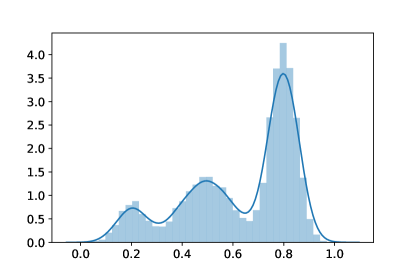
(a) Data generating distribution (kernel density estimate)

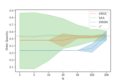
(b) Order Quantity

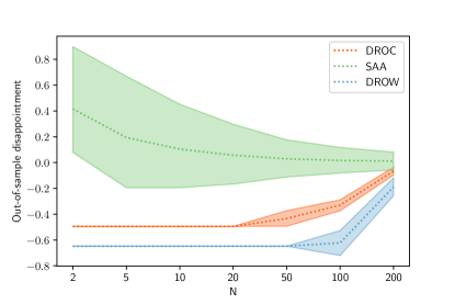
(c) Out-of-sample disappointment

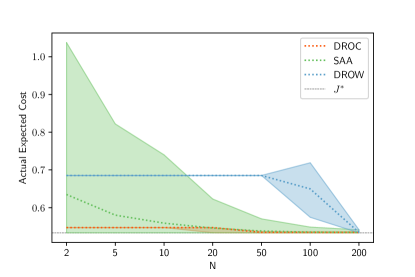
(d) Actual expected cost

Figure 1: Single-item newsvendor problem: (Approximate) true data-generating distribution, order quantity and performance metrics

4.1.2 The multi-item newsvendor problem

In this section, we carry out an analysis similar to that of Subsection 4.1.1, but for the multi-item newsvendor problem, which can be formulated as follows:

$$\inf_{\mathbf{x}\geqslant\mathbf{0}}\mathbb{E}_{Q}\sum_{l=1}^{d}[h_{l}(x_{l}-\xi_{l})^{+}+b_{l}(\xi_{l}-x_{l})^{+}]$$

where $x_{l}$ is the order quantity for the $l$-th item, $Q$ is the joint probability distribution governing the demands for the $d$ items, and $b_{l},h_{l}>0$ are the unit holding cost and the unit backorder cost for the $l$-th item, respectively.

To illustrate our approach in a higher dimensional setting, we consider twenty items, i.e., $d=20$.

We consider the following parameters: $h_{1}=\ldots=h_{10}=2,h_{11}=\ldots=h_{20}=4$, $b_{1}=\ldots=b_{10}=4$; and $b_{11}=\ldots=b_{20}=2$. The demands for the twenty items are assumed to follow a mixture of three multivariate normal distributions $\mathcal{N}_{20}(\boldsymbol{\mu}_{1},\Sigma_{1}),$ $\;\mathcal{N}_{20}(\boldsymbol{\mu}_{2},\Sigma_{2}),\;$ and $\mathcal{N}_{20}(\boldsymbol{\mu}_{3},\Sigma_{3}),\;$ where $\boldsymbol{\mu}_{1}=[3,\ldots,3]\in\mathbb{R}^{20},\ \Sigma_{1}=\textrm{diag}(1,\ldots,1)\in\mathbb{R}^{20\times 20}$; $\boldsymbol{\mu}_{2}=[5,\ldots,5]\in\mathbb{R}^{20},\ \Sigma_{2}=\textrm{diag}(0.5,\ldots,0.5)\in\mathbb{R}^{20\times 20}$; and $\boldsymbol{\mu}_{3}=[7,\ldots,7]\in\mathbb{R}^{20},\ \Sigma_{3}=\textrm{diag}(0.1,\ldots,0.1)\in\mathbb{R}^{20\times 20}$. The weights of the mixture are $\omega_{1}=0.1,\;\omega_{2}=0.65$ and $\omega_{3}=0.25$, respectively. Furthermore, the mixture has been truncated on the hypercube $[0,10]^{20}$.

The values we have used for the parameters $\varepsilon$ and $\rho$ in DROC and DROW are collated in Table 2.

Table 2: Multi-item newsvendor problem: Values for parameters $\varepsilon$, $\rho$ in DROC and $\rho$ in DROW

$N$	DROC		DROW
	$\varepsilon$	$\rho$	$\rho$
2	5	2	60
5	5	2	50
10	4.5	1.5	40
20	4	1	20
50	2.5	0.6	10
100	1.75	0.5	8
200	1.25	0.35	4

Again, for a meaningful and fair comparison, these parameters have been tuned by trial and error in such a way that at most 50 out of the 1000 runs we have carried out for each sample size $N$ yield a positive out-of-sample disappointment. The values for the parameters, which we need to this end, diminish as we gain more information (i.e., as the sample size $N$ grows). Note that, for small sample sizes, for which the available data provide very little information about their true distribution, a great deal of robustness is required to produce highly reliable data-driven solutions. Consequently, it is little wonder that the selected values for $\rho$ in DROC are equal to two, which is the maximum value that the total variation distance between $P$ and $\widehat{P}$ can take on.

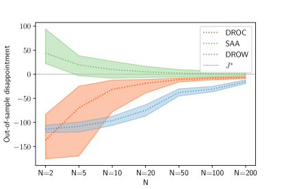
(a) Out-of-sample disappointment

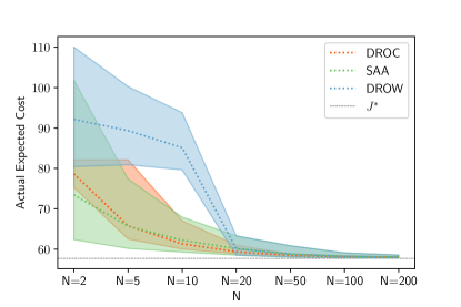
(b) Actual expected cost

Figure 2: Multi-item newsvendor problem: Performance metrics

In the same fashion as in the case of the previous example of the single-item newsvendor problem, Figures  2a and 2b show, for various sample sizes, the box plots pertaining to the out-of-sample disappointment and the actual expected cost associated with each of the considered data-driven approaches, in that order. The results conveyed by these figures confirm our initial conclusions: The ability of our approach DROC to exploit a-priori knowledge of the order among some partition probabilities permits identifying solutions that perform noticeably better out of sample with the same level of confidence. We underline that, in terms of the out-of-sample disappointment, the decision maker seeks a data-driven method $m$ that renders an estimate $\widehat{J}_{N}^{m}$ that results in a positive surprise (i.e., negative disappointment) with a high probability, but that is as close as possible to the cost with full information $J^{*}$. Consequently, the large negative out-of-sample disappointment that the solutions given by DROW feature can be attributed to its over-conservativeness.

In terms of computational time, solving DROC for this instance of the multi-item newsvendor problem, with 20 items, four partitions and a sample size of 200, takes less than a second with CPLEX 12.10 running on a Windows 10 PC with a CPU Intel (R) Core i7-8550U clocking at 1.80 GHz and 8 GB of RAM.

4.2 The problem of a strategic firm competing à la Cournot in a market

Next we consider the problem of a strategic firm competing à la Cournot in a market for an undifferentiated product. This could be the case of, for instance, the electricity market (see, e.g., (gabriel2012complementarity, , Ch. 3) and Ruiz2008 ). Suppose the firm can produce up to one per-unit amount of product at a cost given by $a_{2}x^{2}+a_{1}x+a_{0}$, where $x$ is the per-unit amount of product eventually produced and $a_{0},a_{1}$ and $a_{2}$ are known parameters taking values in $\mathbb{R}^{+}$. Furthermore, assume an inverse residual demand function in the form $\lambda=\alpha-\beta x$, where $\lambda$ is the market clearing price for the product, and $\alpha,\beta\in\mathbb{R}^{+}$ are unknown and uncertain parameters. The firm seeks, therefore, to minimize its cost $(a_{2}x^{2}+a_{1}x+a_{0})-\lambda x$ subject to $x\in[0,1]$. After some basic manipulation, the problem of the firm can be posed as

$$\inf_{x\in[0,1]}\mathbb{E}_{Q}[(-x)\xi+x^{2}]$$

where $\xi=\frac{\alpha-a_{1}}{\beta+a_{2}}$.

The most interesting feature of this example is that, unlike in the aforementioned newsvendor problems, the Lipschitz constant of the objective function $f(x,\xi):=(-x)\xi+x^{2}$ with respect to $\boldsymbol{\xi}$ is dependent on the decision variable $\mathbf{x}$.

We consider that $\xi$ follows a (true) probability distribution given by 10 000 points sampled from a mixture of three Gaussian distributions with variances all equal to $0.3$ and means $\mu_{1}=0,\mu_{2}=1.2$ and $\mu_{3}=2.5$. The weights of the mixture are $\omega_{1}=0.5,\omega_{2}=0.2$ and $\omega=30.3$. Furthermore, the mixture has been truncated (over the interval $[-1.8,3]$. Figure 3a plots the kernel estimate of the data-generating distribution.

As in the previous experiments, we have divided the support $[-1.8,3]$ into four partitions, using the procedure described at the beginning of Section 4. However, in a different way to what we did in the newsvendor examples, here we select parameters $\varepsilon$ and $\rho$ following a procedure that solely relies on the available data, similarly to what is done in MohajerinEsfahani2018 . Essentially, given a desired confidence level $(1-\beta)$ for the finite-sample guarantee (set to 0.85 in our numerical experiments), we need to estimate, using the data sample available only, the parameters $\varepsilon$ and $\rho$ that deliver, at least, this confidence level while yielding the best out-of-sample performance. To this end, we use bootstrapping. The estimator of those parameters is denoted as $param_{N}^{m}(\beta)$, underlining that the number and type of parameters to be estimated depend on the method $m$. The estimation procedure is carried out as follows for each sample of size $N$ (in this experiment, we consider $300$ independent data samples for each size $N$):

1. We construct $kboot$ resamples of size $N$ (with replacement), each playing the role of a different training dataset. Moreover, take those data points that have not been resampled to form a validation dataset (one per resample of size $N$). In our experiments below, we have considered $kboot=50$.

2. For each resample $k=1,\ldots,kboot$ and each candidate value for $param$, get a DRO solution from method $j$ with parameter (or pair of paramaters) $param$ on the $k$-th resample. The resulting optimal decision is denoted as $\widehat{x}^{j,k}_{N}(param)$ and its associated objective value as $\widehat{J}^{j,k}_{N}(param)$. Subsequently, we compute the out-of-sample performance $J(\widehat{x}^{j,k}_{N}(param))$ of the data-driven solution $\widehat{x}^{j,k}_{N}(param)$ over the $k$-th validation dataset.

3. From among the candidate values for $param$ such that $\widehat{J}^{j,k}_{N}(param)$ exceeds the value $J(\widehat{x}^{j,k}_{N}(param))$ in at least $(1-\beta)\times kboot$ different resamples, take the one with the lowest $\frac{\sum_{k=1}^{kboot}{J(\widehat{x}^{j,k}_{N}(param))}}{kboot}$ (that is, with the highest out-of-sample performance averaged over the $kboot$ resamples).

4. Finally, compute the solution given by method $j$ with parameter $param^{\beta,j}_{N}$, $\widehat{x}^{j}_{N}:=\widehat{x}^{j}_{N}(param^{\beta,j}_{N})$ and the respective certificate $\widehat{J}^{j}_{N}:=\widehat{J}^{j}_{N}(param^{\beta,j}_{N})$.

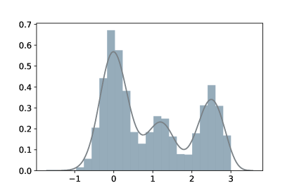
(a) Data generating distribution (kernel density estimate)

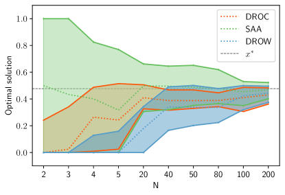
(b) Optimal solution

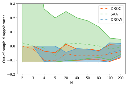
(c) Out-of-sample disappointment

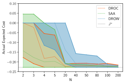
(d) Actual expected cost

Figure 3: Strategic firm problem: (Approximate) true data-generating distribution, optimal solution and performance metrics

As for the newsvendor examples, Figures 3b, 3c, and 3d show, for various sample sizes, the box plots pertaining to the optimal decision, the out-of-sample disappointment and the actual expected cost associated with each of the considered data-driven approaches, in that order. Once again, the results conveyed by these figures confirm our previous conclusions: Our approach DROC is able to leverage a-priori knowledge of the order among some partition probabilities to deliver solutions that perform significantly better out of sample for the same level of confidence. Furthermore, we see that the decision computed by the proposed method DROC converges to the true optimal solution (with complete information) faster than the solutions provided by the other methods.

5 Conclusions

In this paper, we have presented a novel framework for data-driven distributionally robust optimization (DRO) based on optimal transport theory in combination with order cone constraints to leverage a-priori information on the true data-generating distribution. Motivated by the reported over-conservativeness of the traditional DRO approach based on the Wasserstein metric, we have formulated an ambiguity set able to incorporate information about the order among the probabilities that the true distribution of the problem’s uncertain parameters assigns to some subregions of its support set. Our approach can accomodate a wide range of shape information (such as that related to monotonicity or multi-modality) in a practical and intuitive way. Moreover, under mild assumptions, the resulting distributionally robust optimization problem can be, in fact, reformulated as a finite convex problem where the a-priori information (expressed through the order cone constraints) are cast as linear constraints as opposed to the more computationally challenging formulations that exist in the literature. Furthermore, our approach is supported by theoretical performance guarantees and is capable of turning the provided information into solutions with increased reliability and improved performance, as illustrated by the numerical experiments we have prepared based on the well-known newsvendor problem and the problem of a strategic firm competing á la Cournot in a market for a homogeneous product.

Compliance with ethical standards

Funding    This research has received funding from the European Research Council (ERC) under the European Union’s Horizon 2020 research and innovation programme (grant agreement no. 755705). This work was also supported in part by the Spanish Ministry of Economy, Industry and Competitiveness and the European Regional Development Fund (ERDF) through project ENE2017-83775-P.

Conflict of interest    The authors declare that they have no conflict of interest.

References

- (1) CPLEX Optimizer-IBM. Available (online): (2019). https://www.ibm.com/analytics/cplex-optimizer
- (2) Pyomo. Available (online): (2019). http://www.pyomo.org/
- (3) Andersson, J., Jörnsten, K., Nonås, S.L., Sandal, L., Ubøe, J.: A maximum entropy approach to the newsvendor problem with partial information. European Journal of Operational Research 228(1), 190–200 (2013). DOI 10.1016/j.ejor.2013.01.031. URL https://linkinghub.elsevier.com/retrieve/pii/S0377221713000787
- (4) Bayraksan, G., Love, D.K.: Data-Driven stochastic programming using phi-divergences. In: The Operations Research Revolution, pp. 1–19. INFORMS (2015). DOI 10.1287/educ.2015.0134. URL http://pubsonline.informs.org/doi/10.1287/educ.2015.0134
- (5) Ben-Tal, A., den Hertog, D., De Waegenaere, A., Melenberg, B., Rennen, G.: Robust solutions of optimization problems affected by uncertain probabilities. Management Science 59(2), 341–357 (2013). DOI 10.1287/mnsc.1120.1641. URL http://pubsonline.informs.org/doi/abs/10.1287/mnsc.1120.1641
- (6) Ben-Tal, A., den Hertog, D., Vial, J.P.: Deriving robust counterparts of nonlinear uncertain inequalities. Mathematical Programming 149(1-2), 265–299 (2015). DOI 10.1007/s10107-014-0750-8. URL http://link.springer.com/10.1007/s10107-014-0750-8
- (7) Bertsimas, D., Gupta, V., Kallus, N.: Data-driven robust optimization. Mathematical Programming 167(2), 235–292 (2018). DOI 10.1007/s10107-017-1125-8. URL http://link.springer.com/10.1007/s10107-017-1125-8
- (8) Bertsimas, D., Gupta, V., Kallus, N.: Robust sample average approximation. Mathematical Programming 171(1-2), 217–282 (2018). DOI 10.1007/s10107-017-1174-z. URL http://link.springer.com/10.1007/s10107-017-1174-z
- (9) Bhattacharya, B.: Testing multinomial parameters under order restrictions. Communications in Statistics - Theory and Methods 26(8), 1839–1865 (1997). DOI 10.1080/03610929708832017. URL http://www.tandfonline.com/doi/abs/10.1080/03610929708832017
- (10) Blanchet, J., Kang, Y., Murthy, K., Zhang, F.: Data-driven optimal transport cost selection for distributionally robust optimization. In: 2019 Winter Simulation Conference (WSC), pp. 3740–3751 (2019). DOI 10.1109/WSC40007.2019.9004785
- (11) Blanchet, J., Kang, Y., Zhang, F., He, F., Hu, Z.: Doubly robust data‐driven distributionally robust optimization. In: Applied Modeling Techniques and Data Analysis 1, pp. 75–90. Wiley (2021). DOI 10.1002/9781119821588.ch4. URL https://onlinelibrary.wiley.com/doi/10.1002/9781119821588.ch4
- (12) Borwein, J.M., Hamilton, C.H.: Symbolic Fenchel conjugation. Mathematical Programming 116(1-2), 17–35 (2009). DOI 10.1007/s10107-007-0134-4. URL http://link.springer.com/10.1007/s10107-007-0134-4
- (13) Boyd, S., Vandenberghe, L.: Convex Optimization (2004). DOI 10.1017/CBO9780511804441
- (14) Chen, R., Paschalidis, I.C.: A robust learning approach for regression models based on distributionally robust optimization. Journal of Machine Learning Research 19(13), 1–48 (2018). URL http://jmlr.org/papers/v19/17-295.html
- (15) Chen, X., Lin, Q., Xu, G.: Distributionally robust optimization with confidence bands for probability density functions (2019). URL http://arxiv.org/abs/1901.02169
- (16) Chen, Z., Sim, M., Xiong, P.: Robust stochastic optimization made easy with RSOME. Management Science 66(8), 3329–3339 (2020). DOI 10.1287/mnsc.2020.3603. URL http://pubsonline.informs.org/doi/10.1287/mnsc.2020.3603
- (17) Choi, T.M. (ed.): Handbook of Newsvendor Problems, International Series in Operations Research & Management Science, vol. 176. Springer New York, New York, NY (2012). DOI 10.1007/978-1-4614-3600-3. URL http://link.springer.com/10.1007/978-1-4614-3600-3
- (18) Cisneros-Velarde, P., Petersen, A., Oh, S.Y.: Distributionally robust formulation and model selection for the graphical lasso. In: S. Chiappa, R. Calandra (eds.) Proceedings of the Twenty Third International Conference on Artificial Intelligence and Statistics, Proceedings of Machine Learning Research, vol. 108, pp. 756–765. PMLR, Online (2020). URL http://proceedings.mlr.press/v108/cisneros20a.html
- (19) Dangeti, P.: Statistics for machine learning: Techniques for exploring supervised, unsupervised, and reinforcement learning models with Python and R. Packt Publishing (2017)
- (20) Delage, E., Ye, Y.: Distributionally robust optimization under moment uncertainty with application to data-driven problems. Operations Research 58(3), 595–612 (2010). DOI 10.1287/opre.1090.0741. URL http://pubsonline.informs.org/doi/abs/10.1287/opre.1090.0741
- (21) Duchi, J.C., Glynn, P.W., Namkoong, H.: Statistics of robust optimization: A generalized empirical likelihood approach. Mathematics of Operations Research p. moor.2020.1085 (2021). DOI 10.1287/moor.2020.1085. URL http://pubsonline.informs.org/doi/10.1287/moor.2020.1085
- (22) Erdoğan, E., Iyengar, G.: Ambiguous chance constrained problems and robust optimization. Mathematical Programming 107(1-2), 37–61 (2006). DOI 10.1007/s10107-005-0678-0. URL http://link.springer.com/10.1007/s10107-005-0678-0
- (23) Fournier, N., Guillin, A.: On the rate of convergence in Wasserstein distance of the empirical measure. Probability Theory and Related Fields 162(3-4), 707–738 (2015). DOI 10.1007/s00440-014-0583-7. URL http://link.springer.com/10.1007/s00440-014-0583-7
- (24) Gabriel, S.A., Conejo, A.J., Fuller, J.D., Hobbs, B.F., Ruiz, C.: Complementarity modeling in energy markets, vol. 180. Springer Science & Business Media (2012)
- (25) Gallego, G., Moon, I.: The distribution free newsboy problem: Review and extensions. The Journal of the Operational Research Society 44(8), 825 (1993). DOI 10.2307/2583894. URL https://www.jstor.org/stable/2583894?origin=crossref
- (26) Gao, R., Kleywegt, A.J.: Distributionally robust stochastic optimization with Wasserstein distance (2016). URL https://arxiv.org/abs/1604.02199
- (27) Gao, R., Kleywegt, A.J.: Distributionally robust stochastic optimization with dependence structure (2017). URL http://arxiv.org/abs/1701.04200
- (28) Graf, S., Luschgy, H.: Foundations of Quantization for Probability Distributions, Lecture Notes in Mathematics, vol. 1730. Springer Berlin Heidelberg, Berlin, Heidelberg (2000). DOI 10.1007/BFb0103945. URL http://link.springer.com/10.1007/BFb0103945
- (29) Guo, S., Xu, H.: Distributionally robust shortfall risk optimization model and its approximation. Mathematical Programming 174(1), 473–498 (2019). DOI 10.1007/s10107-018-1307-z. URL https://doi.org/10.1007/s10107-018-1307-z
- (30) Hanasusanto, G.A., Kuhn, D., Wallace, S.W., Zymler, S.: Distributionally robust multi-item newsvendor problems with multimodal demand distributions. Mathematical Programming 152(1-2), 1–32 (2015). DOI 10.1007/s10107-014-0776-y. URL http://link.springer.com/10.1007/s10107-014-0776-y
- (31) Ji, R., Lejeune, M.A.: Data-driven optimization of reward-risk ratio measures. INFORMS Journal on Computing p. ijoc.2020.1002 (2020). DOI 10.1287/ijoc.2020.1002. URL http://pubsonline.informs.org/doi/10.1287/ijoc.2020.1002
- (32) Keith, A.J., Ahner, D.K.: A survey of decision making and optimization under uncertainty. Annals of Operations Research 300(2), 319–353 (2021). DOI 10.1007/s10479-019-03431-8. URL https://link.springer.com/10.1007/s10479-019-03431-8
- (33) Kuhn, D., Esfahani, P.M., Nguyen, V.A., Shafieezadeh-Abadeh, S.: Wasserstein distributionally robust optimization: Theory and applications in machine learning. In: Operations Research & Management Science in the Age of Analytics, pp. 130–166. INFORMS (2019). DOI 10.1287/educ.2019.0198. URL http://pubsonline.informs.org/doi/10.1287/educ.2019.0198
- (34) Lam, H., Mottet, C.: Tail analysis without parametric models: A worst-case perspective. Operations Research 65(6), 1696–1711 (2017). DOI 10.1287/opre.2017.1643. URL http://pubsonline.informs.org/doi/10.1287/opre.2017.1643
- (35) Li, B., Jiang, R., Mathieu, J.L.: Ambiguous risk constraints with moment and unimodality information. Mathematical Programming 173(1-2), 151–192 (2019). DOI 10.1007/s10107-017-1212-x. URL http://link.springer.com/10.1007/s10107-017-1212-x
- (36) Liu, J., Chen, Z., Lisser, A., Xu, Z.: Closed-form optimal portfolios of distributionally robust mean-CVaR problems with unknown mean and variance. Applied Mathematics & Optimization 79(3), 671–693 (2019). DOI 10.1007/s00245-017-9452-y. URL http://link.springer.com/10.1007/s00245-017-9452-y
- (37) Liu, Q., Wu, J., Xiao, X., Zhang, L.: A note on distributionally robust optimization under moment uncertainty. Journal of Numerical Mathematics 26(3), 141–150 (2018). DOI 10.1515/jnma-2017-0020. URL https://www.degruyter.com/document/doi/10.1515/jnma-2017-0020/html
- (38) Liu, Y.: Discrete Approximation Scheme in Distributionally Robust Optimization. Numerical Mathematics: Theory, Methods and Applications 14(2), 285–320 (2021). DOI 10.4208/nmtma.OA-2020-0125. URL http://global-sci.org/intro/article_detail/nmtma/18601.html
- (39) Lucchetti, R.: Convexity and Well-Posed Problems. CMS Books in Mathematics. Springer New York, New York, NY (2006). DOI 10.1007/0-387-31082-7. URL http://link.springer.com/10.1007/0-387-31082-7
- (40) McLachlan, G., Peel, D.: Finite Mixture Models. Wiley Series in Probability and Statistics. John Wiley & Sons, Inc., Hoboken, NJ, USA (2000). DOI 10.1002/0471721182. URL http://doi.wiley.com/10.1002/0471721182
- (41) Mehrotra, S., Papp, D.: A cutting surface algorithm for semi-infinite convex programming with an application to moment robust optimization. SIAM Journal on Optimization 24(4), 1670–1697 (2014). DOI 10.1137/130925013. URL http://epubs.siam.org/doi/10.1137/130925013
- (42) Mohajerin Esfahani, P., Kuhn, D.: Data-driven distributionally robust optimization using the Wasserstein metric: performance guarantees and tractable reformulations. Mathematical Programming 171(1-2), 115–166 (2018). DOI 10.1007/s10107-017-1172-1
- (43) Nakao, H., Shen, S., Chen, Z.: Network design in scarce data environment using moment-based distributionally robust optimization. Computers & Operations Research 88, 44–57 (2017). DOI 10.1016/j.cor.2017.07.002. URL https://linkinghub.elsevier.com/retrieve/pii/S0305054817301661
- (44) Namkoong, H., Duchi, J.C.: Stochastic gradient methods for distributionally robust optimization with f-divergences. In: D.D. Lee, M. Sugiyama, U.V. Luxburg, I. Guyon, R. Garnett (eds.) Advances in Neural Information Processing Systems 29, pp. 2208–2216. Curran Associates, Inc. (2016).
- (45) Németh, A., Németh, S.: Isotonic regression and isotonic projection. Linear Algebra and its Applications 494, 80 – 89 (2016). DOI https://doi.org/10.1016/j.laa.2016.01.006. URL http://www.sciencedirect.com/science/article/pii/S0024379516000082
- (46) Pando, V., San-José, L.A., García-Laguna, J., Sicilia, J.: A newsboy problem with an emergency order under a general backorder rate function. Omega 41(6), 1020–1028 (2013). DOI 10.1016/j.omega.2013.01.003. URL https://linkinghub.elsevier.com/retrieve/pii/S0305048313000121
- (47) Pando, V., San-José, L.A., García-Laguna, J., Sicilia, J.: Some general properties for the newsboy problem with an extraordinary order. TOP 22(2), 674–693 (2014). DOI 10.1007/s11750-013-0287-7. URL http://link.springer.com/10.1007/s11750-013-0287-7
- (48) Pedregosa, F., Varoquaux, G., Gramfort, A., Michel, V., Thirion, B., Grisel, O., Blondel, M., Prettenhofer, P., Weiss, R., Dubourg, V., Vanderplas, J., Passos, A., Cournapeau, D., Brucher, M., Perrot, M., Duchesnay, E.: Scikit-learn: Machine learning in python. J. Mach. Learn. Res. 12, 2825–2830 (2011). URL http://dl.acm.org/citation.cfm?id=1953048.2078195
- (49) Rahimian, H., Bayraksan, G., Homem-de Mello, T.: Identifying effective scenarios in distributionally robust stochastic programs with total variation distance. Mathematical Programming 173(1-2), 393–430 (2019). DOI 10.1007/s10107-017-1224-6. URL http://link.springer.com/10.1007/s10107-017-1224-6
- (50) Rahimian, H., Mehrotra, S.: Distributionally Robust Optimization: A Review (2019). URL http://arxiv.org/abs/1908.05659
- (51) Roos, E., den Hertog, D., Ben-Tal, A., de Ruiter, F., Zhen, J.: Approximation of hard uncertain convex inequalities (2018). URL http://www.optimization-online.org/DB_HTML/2018/06/6679.html
- (52) Ruiz, C., Conejo, A., García-Bertrand, R.: Some analytical results pertaining to Cournot models for short-term electricity markets. Electric Power Systems Research 78(10), 1672–1678 (2008). DOI 10.1016/j.epsr.2008.02.008. URL https://linkinghub.elsevier.com/retrieve/pii/S0378779608000692
- (53) Santambrogio, F.: Optimal Transport for Applied Mathematicians. Birkäuser Basel (2015). DOI 10.1007/978-3-319-20828-2
- (54) Scarf, H.: A min-max solution of an inventory problem. Studies in The Mathematical Theory of Inventory and Production (1958). URL http://ci.nii.ac.jp/naid/10021308995/en/
- (55) Shafieezadeh-Abadeh, S., Kuhn, D., Esfahani, P.M.: Regularization via mass transportation. Journal of Machine Learning Research 20(103), 1–68 (2019). URL http://jmlr.org/papers/v20/17-633.html
- (56) Shapiro, A.: On duality theory of conic linear problems. In: M.Á. Goberna, M.A. López (eds.) Semi-Infinite Programming, Nonconvex Optimization and Its Applications, pp. 135–165. Springer US (2001). DOI 10.1007/978-1-4757-3403-4˙7. URL https://link.springer.com/chapter/10.1007/978-1-4757-3403-4_7
- (57) Silvapulle, M.J., Sen, P.K.: Constrained Statistical Inference: Inequality, Order, and Shape Restrictions. Wiley Series in Probability and Statistics. John Wiley & Sons, Inc., Hoboken, NJ, USA (2011). DOI 10.1002/9781118165614. URL http://doi.wiley.com/10.1002/9781118165614
- (58) Sion, M.: On general minimax theorems. Pacific Journal of Mathematics 8(1), 171–176 (1958). DOI 10.2140/pjm.1958.8.171. URL http://msp.org/pjm/1958/8-1/p14.xhtml
- (59) Villani, C.: Optimal Transport: Old and New. Grundlehren der mathematischen Wissenschaften. Springer Berlin Heidelberg (2008)
- (60) Wang, C., Gao, R., Qiu, F., Wang, J., Xin, L.: Risk-based distributionally robust optimal power flow with dynamic line rating. IEEE Transactions on Power Systems 33(6), 6074–6086 (2018). DOI 10.1109/TPWRS.2018.2844356. URL https://ieeexplore.ieee.org/document/8373738/
- (61) Wang, Z., Glynn, P.W., Ye, Y.: Likelihood robust optimization for data-driven problems. Computational Management Science 13(2), 241–261 (2016). DOI 10.1007/s10287-015-0240-3. URL http://link.springer.com/10.1007/s10287-015-0240-3
- (62) Xie, W.: On distributionally robust chance constrained programs with Wasserstein distance. Mathematical Programming 186(1-2), 115–155 (2021). DOI 10.1007/s10107-019-01445-5. URL http://link.springer.com/10.1007/s10107-019-01445-5
- (63) Xin, L., Goldberg, D.A.: Time (in)consistency of multistage distributionally robust inventory models with moment constraints. European Journal of Operational Research 289(3), 1127–1141 (2021). DOI 10.1016/j.ejor.2020.07.041. URL https://linkinghub.elsevier.com/retrieve/pii/S0377221720306676
- (64) Yao, L., Wang, X., Duan, C., Wu, X., Zhang, W.: Risk-based distributionally robust energy and reserve dispatch with Wasserstein-moment metric. In: 2018 IEEE Power & Energy Society General Meeting (PESGM), pp. 1–5. IEEE (2018). DOI 10.1109/PESGM.2018.8586296. URL https://ieeexplore.ieee.org/document/8586296/
- (65) Yue, M.C., Kuhn, D., Wiesemann, W.: On Linear Optimization over Wasserstein Balls (2020). URL http://arxiv.org/abs/2004.07162
- (66) Zhao, C., Guan, Y.: Data-driven risk-averse two-stage stochastic program with -structure probability metrics (2015). URL http://www.optimization-online.org/DB_FILE/2015/07/5014.pdf
- (67) Zymler, S., Kuhn, D., Rustem, B.: Distributionally robust joint chance constraints with second-order moment information. Mathematical Programming 137(1-2), 167–198 (2013). DOI 10.1007/s10107-011-0494-7. URL http://link.springer.com/10.1007/s10107-011-0494-7