Interacting bosons in generalized zig-zag and railroad-trestle models

Abstract

We theoretically study the ground-state phase diagram of strongly interacting bosons on a generalized zig-zag ladder model, the rail-road trestle (RRT) model. By means of analytical arguments in the limits of decoupled chains and the case of vanishing fillings as well as extensive DMRG calculations we examine the rich interplay between frustration and interaction for various parameter regimes. We distinguish three different cases, the fully frustrated RRT model where the dispersion relation becomes doubly degenerate and an extensive chiral superfluid regime is found, the anti-symmetric RRT with alternating $\pi$ and $0$ fluxes through the ladder plaquettes and the sawtooth limit, which is closely related to the latter case. We study detailed phase diagrams which include besides different single component superfluids, the chiral superfluid phases, the two component superfluids and different gaped phases, with dimer and a charge-density wave order.

I Introduction

Frustrated systems are one of the most interesting as well as widely explored yet still most challenging problems in the field of condensed matter physics. Frustration in one and quasi-one dimensional systems, such as quasi one-dimensional magnetic materials Hase et al. (2004); Masuda et al. (2005); Drechsler et al. (2007); Vasiliev et al. (2018), are of paramount importance due to the strong correlations which in interplay with the geometric frustration lead to non-trivial and intriguing physics. Theoretically in particular the $J_{1}$-$J_{2}$ spin model, with a frustrated next-nearest neighbour tunnelling amplitude $J_{2}$, has been extensively studied during the recent decades and important milestones include the famous analytical solution for the isotropic spin-$1/2$ $J_{1}$-$J_{2}$-model by Majumdar and Ghosh Majumdar and Ghosh (1969) or the Ising type phase transition between the critical Luttinger-liquid XY and the gapped dimerized (D) phase Haldane (1982); Okamoto and Nomura (1992). Detailed ground-state properties in different regimes and for various spins $S\geq 1/2$ have been discussed both numerically and analytically  Kolezhuk (2000); Lecheminant et al. (2001); Vekua et al. (2003); Hikihara et al. (2000, 2001); Hikihara (2002); Kolezhuk et al. (2012) in the ferromagnetic Hikihara et al. (2008) as well as antiferromagnetic regime Hikihara and Furusaki (2004); Furukawa et al. (2010); Azimi et al. (2014).

Recent experiments on ultracold quantum gases in optical lattices Aidelsburger et al. (2011); Struck et al. (2012); Miyake et al. (2013); Aidelsburger et al. (2013), as well as irradiated graphene Oka and Aoki (2009); Wang et al. (2013) or photonic lattices Hafezi et al. (2011); Rechtsman et al. (2013); Mittal et al. (2016), have paved the path towards the manipulation of lattice frustration to establish a situation to mimic condensed matter phenomena. The seminal experimental emulation of geometric frustration in a triangular optical lattice by Struck et al. Struck et al. (2012) has attracted enormous interest to understand the physics of lattice frustration at ultra low temperature. In recent years various interesting predictions have been made in the context of geometric frustration in low dimensional lattices such as zig-zag lattices which resembles the quantum $J_{1}$-$J_{2}$ model under proper conditions: Studies on systems of bosons in frustrated zig-zag lattices have predicted the presence of chiral phases Greschner et al. (2013) which arise due the spontaneously breaking of the inversion symmetry of the system. On the other hand it has been shown that the supersolid phases can be stabilized in a system of hardcore bosons in a frustrated zig-zag lattice with dipole-dipole interactions Mishra et al. (2014, 2015a). Recently, interesting extensions to an arbitrary rectified flux have been discussed Anisimovas et al. (2016).

A natural extension of the zig-zag ladder is to allow for a difference in the tunnelling amplitudes between upper and lower leg. One of the interesting variant of the frustrated zig-zag lattice model is the sawtooth model which exhibits non-trivial physics due to the existence of a flat band. It has been shown that a solid order emerges at quarter filling in a frustrated one dimensional sawtooth model by Huber and Altman Huber and Altman (2010) by means of an effective model valid in the flat-band regime. Interestingly, a numerical analysis of this model has shown that also a supersolid phase can be stabilized in the absence of long-range interactions Mishra et al. (2015b). The existence of this supersolid phase can be attributed to the presence of alternating flux in the consecutive plaquettes of the lattice which occurs due the lattice geometry.

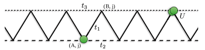
Figure 1: Railroad Trestle (RRT) lattice which is a most general model for zig-zag ladder with tunneling amplitudes $t_{1}$, $t_{2}$ and $t_{3}$.

In this paper we widen the scope of study to the general railroad-trestle (RRT) model where one considers different hopping amplitudes in the legs of the ladder as shown in the Fig 1. The RRT model and its variant the sawtooth model have been extensively analyzed in the context of fermions Tonegawa and Harada (1987); Sarkar and Sen (2002); Capriotti et al. (2003); Nakane et al. (2006); Sen et al. (1996), but the bosonic or spin analog of this model is still a open problem. In this paper we present a detailed analysis of the ground-state properties of the bosonic RRT model in different limits to understand the effects of geometric frustration. We study three major variants of the RRT model using different analytical arguments in the limiting cases. The exact ground state properties are studied using the density matrix renormalization group (DMRG) method White (1992); Schollwöck (2011).

II Model

The RRT model as sketched in Fig. 1 is defined by the following Hamiltonian

$$H(t_{1},t_{2},t_{3})= -t_{1}\sum_{i}(a_{i}^{\dagger}b_{i}^{\phantom{\dagger}}+b_{i}^{\dagger}a_{i+1}^{\phantom{\dagger}}+\text{H.c.})$$

$$-t_{2}\sum_{i}(a_{i}^{\dagger}a_{i+1}^{\phantom{\dagger}}+\text{H.c.})$$

$$-t_{3}\sum_{i}(b_{i}^{\dagger}b_{i+1}^{\phantom{\dagger}}+\text{H.c.})$$ (1)

Here, $a_{i}^{(\dagger)}$ and $b_{i}^{(\dagger)}$ are the bosonic annihilation(creation) operators for the upper (B) and lower (A) legs respectively (see Fig. 1). While $t_{1}$ is the hopping amplitude between the legs, $t_{2}$ and $t_{3}$ correspond to the hoppings along the leg-A and leg-B respectively. The local onsite interactions can be introduced in the model as

$$H_{int}=\frac{U}{2}\sum_{\nu\in\{A,B\},i}n^{\nu}_{i}(n^{\nu}_{i}-1),$$ (2)

where $U$ is the onsite repulsion and $n^{\nu}_{i}$ stands for the number operators at sites. In the following we assume the energy unit $t_{1}=1$ (unless stated otherwise) making all other physical quantities dimensionless. The primary focus of this work is to study the ground state properties of the Model (1) in the limit of hardcore bosons ($U\to\infty$) for different values of $t_{2}$ and $t_{3}$ considering the frustrated regime i.e. $t_{2}<0$. It is now useful to introduce a dimensionless parameter

$$\delta=t_{3}/t_{2}\,.$$ (3)

The remaining part of the paper is organized as follows. In the subsections of this section we analyze two limiting cases of the Model (1) such as the single particle spectrum and the limit of two decoupled chains i.e. when $|t_{1}|\ll|t2|,~{}|t3|$. In the following sections we discuss three different families of parameters: Section (III) is devoted for the fully frustrated RRT(FF-RRT) model with $\pi$-$\pi$ flux arrangements, i.e. $t_{3}<0$. Sec. (IV) constitutes the discussion on the $\pi$-$0$ flux case, with $t_{3}>0$. In Sec. (V) we analyze the sawtooth ladder model i.e. $t_{3}=0$. In the end we conclude in Sec. (IV).

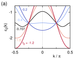
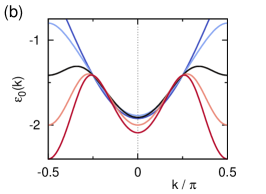
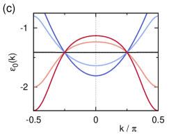
Figure 2: Single particle energies of the RRT model with (a) $\pi$-$\pi$-case $\delta=t_{2}/t_{3}=1/2$, (b) $0-\pi$ case $\delta=-1/2$, and (c) sawtooth case $\delta=0$. We choose $t_{2}=-0.2$, $-0.4$, $-0.707$,$-1.0$, $-1.2$ (from top to bottom at $k\to\pi/2$).

II.1 Single particle spectrum

It is instructive to start the discussion of the physics of Model (1) from the single particle perspective. The kinetic part can be written in momentum space $k$ as

$$H=-\sum_{k}\left(\!\!\begin{array}[]{c}a_{k}\\ b_{k}\\ \end{array}\!\!\right)^{\dagger}\!\left(\begin{array}[]{cc}2t_{2}\cos(k)&t_{1}\left(1+e^{ik}\right)\\ t_{1}\left(1+e^{-ik}\right)&2t_{3}\cos(k)\\ \end{array}\right)\left(\!\!\begin{array}[]{c}a_{k}\\ b_{k}\\ \end{array}\!\!\right)$$ (10)

Diagonalizing the $2\times 2$ matrix one obtains the energy dispersion for generally two bands as

$$\varepsilon_{0,1}(k)=\pm\sqrt{4t_{1}^{2}\cos^{2}\left(\frac{k}{2}\right)+(t_{2}-t_{3})^{2}\cos^{2}(k)}$$

$$-(t_{2}+t_{3})\cos(k)$$ (11)

with the new creation and annihilation operators $\alpha_{k}=\cos(\theta_{k})a_{k}+\sin(\theta_{k})a_{k}$ and $\beta_{k}=\sin(\theta_{k})a_{k}-\cos(\theta_{k})a_{k}$, with the corresponding Bolgoliubov coefficients $\theta_{k}$. This expression for $\varepsilon_{0}(k)$ can give us insight into the physics of the system.

In general we are interested in three different cases, distinguished by the parameter $\delta=t_{3}/t_{2}$ (setting $t_{2}<0$). In Fig. 2 we show examples of the lowest band $\varepsilon_{0}(k)$ dispersion for three different cases of $\delta$ and for each case we consider different values of $t_{2}$. For $\delta>0$, the flux through every unit-cell is equal to $\pi$ (Fig. 2 (a)). Here one finds a parameter regime in which the dispersion exhibits a doubly degenerate minimum. For the case $\delta=1$ this model corresponds to the symmetric zig-zag ladder $H_{S}=H(t_{1},t_{2},t_{2})$ resembling the $J_{1}-J_{2}$ model, which has been studied extensively in the literature as discussed in the introduction. In this case, the $\varepsilon_{0}(k)$ possesses single and double degenerate minima as a function of $t_{2}$ and becomes quartic ($\sim(k-Q)^{4}$) at the so called Lifshitz-transition point, $t_{2}=-1/4$.

While for small values of $-t_{2}\ll 1$ the single minimum of the dispersion relation is at $k=0$, for large values of $-t_{2}\gg 1$ and $\delta\neq 1$ the dispersion relation will generally exhibit a minimum at $k=\pi/2$. We will later on associate two different single component Luttinger-liquid phases with these two dispersion minima, the superfluid at $k=0$ which we call the SF₀ phase, and the corresponding SF_π/2 phase at $k=\pi/2$. The situations in which the dispersion exhibits a degenerate minimum will give rise to further interesting quantum phases discussed below in detail.

On the other hand, for $\delta<0$, only every second plaquette exhibits a $\pi$ flux while the others have zero flux. In this case, instead of a Lifshitz transition with a quartic dispersion relation, the single-particle spectrum becomes degenerate only at a special point $\delta=\delta_{c}$ as shown in Fig. 2 (b). This is, however, sufficient to induce a number of interesting effects in the ground state phase diagram which we will discuss later on.

Finally, for the special case of $\delta=0$ the system is called a sawtooth ladder. This exhibits a flat lowest band at $t_{2}=-1/\sqrt{2}$ as shown in Fig. 2 (c). Although apparently the sawtooth limit is the intermediate between the previous two cases i.e. $\delta<0$ and $\delta>0$, this situation resembles to some extent the $\pi$-$0$-flux systems as one bond is absent Mishra et al. (2015b). The many-body physics which translates from this kind of band picture will be systematically discussed in the following sections.

II.2 Limit of decoupled chains $|t_{1}|\ll|t_{2}|,|t_{3}|$

The phase diagram in the frustrated regime can be understood from the limit of two decoupled chains which is $|t_{1}|\ll|t_{2}|,|t_{3}|$ or in other words when $t_{1}\to 0$ the two chains are independent. For an asymmetric system, i.e. if $t_{2}\neq t_{3}$, both chains will in general be occupied by different particle densities. In the decoupling limit we expect only one chain with the larger tunneling amplitude $t_{3}>t_{2}$ to be occupied, if the density $n$ is small enough. This can be seen from a mapping to free fermions, which results in two bands $-2t_{2}\cos(k)$ and $-2t_{3}\cos(k)$. Only the lowest band is occupied for

$$n<\arccos\bigg{(}\frac{t_{2}}{t_{3}}\bigg{)}/2\pi.$$ (12)

For larger fillings the system enters a regime with two critical Luttinger liquids or two-superfluids (2SF), characterized by a central charge $c=2$ Calabrese and J. Cardy (2004).

The effect of a perturbative coupling between the two chains i.e. by adding a small zig-zag hopping $H_{zz}=H(t_{1},0,0)$ is best described by a bosonization treatment of this case as presented in Ref. Lecheminant et al. (2001) for the symmetric case $\delta=1$. For each sub-chain we introduce two pairs of bosonic fields ($\theta_{1},\phi_{1}$) and ($\theta_{2},\phi_{2}$). After forming symmetric and anti-symmetric combinations $\theta_{\pm}=(\theta_{1}\pm\theta_{2})/\sqrt{2\pi}$, $\phi_{\pm}=\sqrt{\pi}(\phi_{1}\pm\phi_{2})/\sqrt{2}$ the effective low-energy model Greschner et al. (2013) is given by

$$H=\sum_{\alpha=\pm}\frac{v_{\alpha}}{2}\left[\frac{(\partial_{x}\phi_{\alpha})^{2}}{K_{\alpha}}+K_{\alpha}(\partial_{x}\theta_{\alpha})^{2}\right]$$

$$+\lambda\partial_{x}\theta_{+}\sin\sqrt{2\pi}\theta_{-}+\cdots\,.$$ (13)

The last term is relevant and introduces a gap in the anti-symmetric sector $\theta_{-}$, resulting in a finite chirality $O_{\chi}\sim\langle\sin\sqrt{2\pi}\theta_{-}\rangle$ Nersesyan et al. (1998). In the thermodynamic limit it exhibits a non-vanishing local boson current or chirality $\kappa_{i}=\frac{i}{2}(b_{i}^{\dagger}b_{i+1}-{\rm H.c.})$ in the system which is a signature of the chiral superfluid(CSF) phase. In a finite system this locally defined chirality is always zero. However, the CSF phase is clearly characterized by the long-range ordered chirality-chirality correlations defined as

$$O_{\chi}=\lim_{|i-j|\to\infty}\langle{\kappa_{i}\kappa_{j}}\rangle.$$ (14)

It is to be noted that the CSF phase possess a central charge $c=1$ and the 2SF phase does not exhibit a finite chirality.

Interestingly, for the anti-symmetric zig-zag model $H_{A}=H(t_{1},t_{2},-t_{2})$ i.e. with $\delta=-1$, we do not expect this gapping mechanism to work. This can be understood by a simple gauge transformation $a_{j}^{(\dagger)}\to(-1)^{j}a_{j}^{(\dagger)}$, and $b_{j}^{(\dagger)}\to b_{j}^{(\dagger)}$. With this we can map $H_{A}\to H_{S}$, but the zig-zag hopping acquires an oscillating factor

$$H_{zz}\to\sum_{i}(-1)^{i}(a_{i}^{\dagger}b_{i}^{\phantom{\dagger}}-b_{i}^{\dagger}a_{i+1}^{\phantom{\dagger}}+\text{H.c.})$$ (15)

Due to this strong oscillatory term, the perturbation in general becomes irrelevant and the system should stay in the 2SF phase. Only for the case of a certain commensurability $n=1/4$, however, the oscillation may be compensated in a bosonization description, and we may expect the emergence of a gap in the symmetric sector.

Note that the asymmetric case ($t_{2}\neq t_{3}$) may be understood as a combination of the symmetric and antisymmetric zig-zag model i.e. $H=\frac{t_{2}+t_{3}}{2}H_{S}+\frac{t_{2}-t_{3}}{2}H_{A}+H_{zz}$. Hence, we might naively expect the physics arising as a combination of both the effects. In the following we will examine these heuristic arguments by means of more rigorous methods.

III The fully frustrated RRT (FF-RRT) model ($\pi$-$\pi$-flux)

In this section we begin the discussion with the case $\delta>0$ and then we compare our results with the already known case of the symmetric zig-zag chain. First we analyze the physics in the dilute limit and then we extend our calculation by increasing the density.

III.1 Dilute limit

The interplay between local interactions and geometric frustration which gives rise to the various quantum phases can be best understood in the limit of low fillings $n\to 0$ or the dilute limit. In the presence of two non-equivalent minima at $k=\pm Q$ the ground state of a non-interacting boson system is highly degenerate and the effect of interactions becomes crucial which selects a particular ground state. The particles at low energies mainly populate the two dispersion minima at $Q$ and $-Q$. We can interpret them as two different bosonic flavors and map to an effective two component model with intra-species coupling $g_{11}=g_{22}$ between bosons of the same species and inter-species coupling $g_{12}$ between different flavors. Typically two different types of SF ground states may be stabilized: Either the bosons equally occupy both minima, i.e. both flavors are present (the 2SF phase), or one of them is spontaneously selected and a one component SF phase with a spontaneously broken symmetry is realized.

If the intra-species coupling $g_{11}>g_{12}$, a two component Luttinger-liquid phase (2SF) may be realized. In this case both the dispersion minima are equally populated. On the other hand a dominant inter-species coupling $g_{11}<g_{12}$ results a spontaneously broken state with a dominant occupation of the dispersion minimum at $k=Q$ or $k=-Q$.

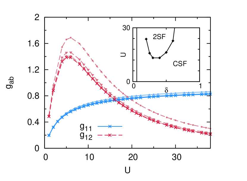
Figure 3: Dilute limit intra-(inter-)particle coupling constants $g_{11}$($g_{12}$) are plotted w.r.t. $U$ for $t_{2}=-0.6$ and $\delta=0.5$. Different curves correspond to (top to bottom) different values of $E_{*}=10^{-2}$, $10^{-3}$, and $10^{-4}$ and the cross-symbol denotes the extrapolation to $E_{*}\to 0$. It can be seen that the value of $g_{11}$ dominates over $g_{12}$ after a critical value of $U$ indicating the 2SF phase. The inset shows the phase transition points between the dominant $g_{11}$ and $g_{12}$ corresponding to the 2SF and the CSF phases respectively as function of $U$ and $\delta$ for $t_{2}=-0.6$. The solid vertical line denotes the Lifsitz transition between SF₀ and frustrated phases. Close to this region our numerical scheme becomes unstable.

While in general it is a useful observation Kolezhuk et al. (2012) that both coupling coefficients, $g_{11}$ and $g_{12}$, may be extracted from the two particle scattering problem on the lattice, here we will follow a slightly different approach. As shown in Kolezhuk et al. (2012) in the dilute limit it is possible to obtain the renormalized intra- and inter-component interactions analytically as an exact solution of the corresponding Bethe-Salpeter equation. A detailed analytical treatment can be found in Ref. Kolezhuk et al. (2012).

For simplicity we will project the interaction to the lowest band. In momentum space the Hamiltonian becomes

$$H=\sum_{k}\epsilon(k)\beta^{\alpha}_{k}(\beta^{\alpha}_{k})^{\dagger}+\frac{1}{2L}\sum_{k,k^{\prime},q}V_{q}(k,k^{\prime})\beta_{k+q}\beta_{k^{\prime}-q}\beta_{k}\beta_{k^{\prime}}$$ (16)

where $V^{\alpha,\beta}_{q}(k,k^{\prime})$ is the interaction between component $\alpha$ and $\beta$ in the momentum representation. For the BH model this is given by

$$V_{q}(k_{1},k_{2})=\frac{U}{2}\left(\cos(\theta_{k_{1}})\cos(\theta_{k_{2}})\cos(\theta_{k_{2}-q})\cos(\theta_{k_{1}+q})\right.$$

$$\left.+\sin(\theta_{k_{1}})\sin(\theta_{k_{2}})\sin(\theta_{k_{2}-q})\sin(\theta_{k_{1}+q})\right)$$ (17)

We obtain the renormalized two-body interactions $\Gamma_{11}$ and $\Gamma_{12}$ in the dilute limit by the following form of the Bethe-Salpeter equations

$$\Gamma_{q}^{11}(E)=V^{11}(Q,0)-\frac{1}{L}\sum_{p}\frac{V^{11}(q,p)\Gamma_{p}^{11}(E)}{\epsilon_{Q+p}+\epsilon_{Q-p}-E}$$ (18)

and

$$\Gamma_{q}^{12}(E)=2V^{12}(q,Q)-\frac{1}{L}\sum_{p}\frac{V^{12}(q,p)\Gamma_{p}^{12}(E)}{2\epsilon_{p}+E}$$ (19)

where $E$ is the total energy of the incoming particles with momentum $k$ and $k^{\prime}$. Here we have introduced the symmetriezed interactions

$$V^{11}(q,p) =\frac{1}{2}\left(V_{q-p}(Q+p,Q-p)+V_{q+p}(Q-p,Q+p)\right)$$

$$V^{12}(q,p) =\frac{1}{2}\left(V_{q-p}(-p,p)+V_{q+p}(-p,p)\right)\,.$$ (20)

$\Gamma_{11}$ and $\Gamma_{12}$ may be related to the bare coupling strengths $g_{11}$ and $g_{12}$ as

$$\frac{1}{\Gamma_{\alpha\beta}(-E_{*})}=\left(\frac{m}{4E_{*}}\right)^{1/2}+\frac{1}{g_{\alpha\beta}}+\mathcal{O}(E_{*}^{1/2}).$$ (21)

which corresponds to an off-shell regularization introducing a negative energy $E_{*}$. For $E_{*}\to 0$, corresponding to the dilute limit this procedure has been shown to be well defined. In the following we directly solve Eqs. (18) and  (19) numerically by introducing a Fourier representation of $\Gamma_{q}^{\alpha\beta}(-E_{*})$ using a discretization of the equation and subsequent fast Fourier transform algorithm. The resulting linear set of equation can be solved using standard methods for finite values $E_{*}>0$ and subsequent extrapolation to $E_{*}\to 0$. This procedure becomes eventually unstable due to the presence of divergences in $\Gamma_{q}^{\alpha\beta}(E_{*})$.

In Fig. 3 we show the coupling constants as function of $U$ for the case $t_{2}/t_{1}=0.6$ and $\delta=0.5$. We extrapolate $g_{\alpha\beta}$ with a third order polynomial to the limit $E_{*}\to 0$. For weak interactions the inter-species couplings dominate. At a finite $U>U_{c}$ we observe a crossing between $g_{11}$ and $g_{12}$ curves and hence, a transition to the intra-species coupling dominated 2SF phase. In the inset of Fig. 3 we show the extracted transition points $U=U_{c}$ as a function of $\delta$ for the case $t_{2}=-0.6$. It can be seen that as the value of $\delta$ increases the CSF phase becomes more robust and survives even in the large $U$ limit.

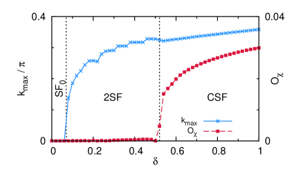
Figure 4: Chirality $O_{\chi}$ and peak position $k_{max}$ of the momentum distribution $n(k)$ for the fully frustrated RRT model as function of $\delta>0$ for small fillings ($n=0.1$, $t_{2}=-0.6$, DMRG data, $L=80$). As $k_{max}\neq 0$ two equivalent maxima at $\pm k_{max}$ are found.

Now we perform numerical DMRG simulations to compare the results with the above findings for the example $t_{2}=-0.6$, also shown in Fig. 3. By considering a system of hardcore bosons with a finite but small filling $n=0.1$, we compute different order parameters such as the chirality order parameter $O_{\chi}$ and the momentum distribution function $n(k)$. The momentum distribution function is defined as

$$n(k)=\frac{1}{L^{2}}\sum_{i,j}{e^{ik(i-j)}}G_{ij}$$ (22)

with the single particle Greens functions $G_{ij}$ along the zig-zag direction of the chain. In Fig. 4 we plot both $O_{\chi}$ and the peak position of $n(k)$ as a function of $\delta$. One may clearly distinguish three regimes. For small values of $\delta$ there exists one peak in the momentum distribution function indicating an SF phase. At some $\delta>\delta_{c1}$ the momentum distribution acquires a double peak structure with $k\neq 0$ which is a signature of the 2SF phase. For $\delta>\delta_{c2}$ the chirality becomes finite and the system enters into the CSF phase.

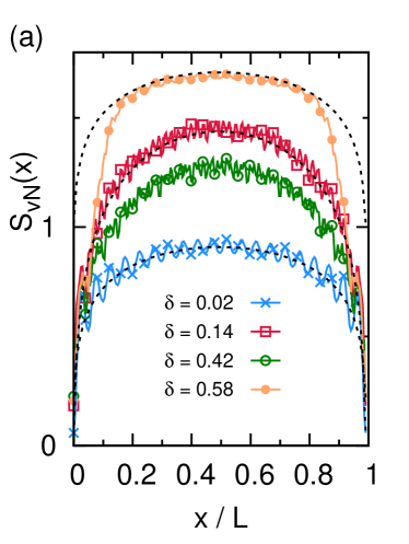
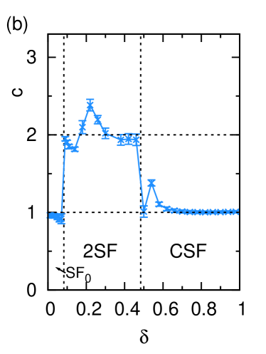
Figure 5: Entanglement scaling for the RRT model using the same parameters as in Fig. 4 (DMRG data, $t_{2}=-0.6$, $L=201$ sites, filling $n=0.1$). (a) Entanglement entropy $S_{vN}(x)$ for different bi-partitions of the system $x$ for various values of $\delta$. The black dashed lines depict a fit to Eq. (23). (b) The extracted central charge $c$ from the fitting procedure.

Moreover, entanglement properties have been shown to provide useful general measure for the detection of quantum phase transitions Osterloh et al. (2002); Vidal et al. (2003). In this regard, we calculate the von-Neumann entropy which is defined as

$$S_{vN,L}(x)=-\mathrm{tr}\left(\rho_{l}\ln\rho_{l}\right)=\frac{c}{6}\ln\left[\frac{L}{\pi}\sin\left(\frac{\pi}{L}l\right)\right]+g\,.$$ (23)

where, $\rho_{l}$ is the reduced density matrix for a subsystem of length $x$ which is plotted as function of $x/L$ in Fig. 5(a). The right part of Eq. (23) is valid for conformally invariant gapless states Vidal et al. (2003); Calabrese and J. Cardy (2004). We fit the expression in the r.h.s. of Eq. (23) to the entanglement entropy curves obtained using the DMRG method as shown in Fig. 5(a). From this we extract the central charge $c$ of the underlying field-theory which is shown in Fig. 5(b). Note, that for the RRT model we perform simulations of system sizes with odd number of sites in order to restore proper inversion symmetry at a central bond. Consistent with our proceeding discussion in Fig. 4 we find that the intermediate non-chiral region exhibits an central charge $c=2$ and hence, can be called a 2SF phase.

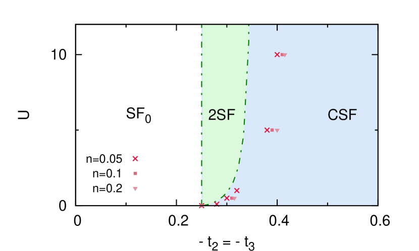
Figure 6: Dilute limit phase diagram of interacting bosons in the symmetric zig-zag model ($\delta=1$). The data points show results for the 2SF to CSF transition from DMRG simulations at finite density $n>0$.

For the special case of a symmetric zig-zag model $\delta=1$ we repeat this analysis in the dilute limit and using the DMRG method and obtain the phase diagram in the $U$-$t_{2}$-plane which is shown in Fig. 6. Close to the Lifsitz transition the 2SF phase is realized. For large frustrations $|t_{2}|>1/\sqrt{8}$ no 2SF phase is found and the system is in a CSF phase, which remains true for the hardcore bosons case. We compare our findings to DMRG results for various fillings and interaction strengths and, as shown in the figure, find a good qualitative agreement between the two results. The symbols in Fig. 6 shows the 2SF-CSF phase boundaries for different densities such as $n=0.05$ (cross), $n=0.1$ (squares) and $n=0.2$ (triangles). Note, that a direct comparison between the two methods may become difficult as for finite dilute systems the order parameter i.e. the chirality vanishes.

III.2 Finite densities

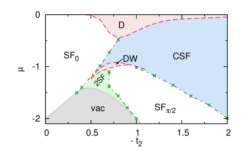
Figure 7: Phase diagram of the FF RRT model for $\delta=1/2$ as function of $t_{2}=2t_{3}$ and the chemical potential $\mu$.

In this subsection we will analyze the complete ground state phase diagram of the asymmetric FF-RRT model for a fixed $\delta=1/2$ as function of the chemical potential $\mu$ to understand the physics at finite densities. From the previous section we find that if $\delta=1/2$ for $\sqrt{\frac{3\sqrt{33}}{2}-\frac{17}{2}}<-t_{2}<1$ the lowest band in Eq. (11) has a two fold degenerate minimum at $Q=\pm\frac{t_{1}\left(3\sqrt{2t_{1}^{2}-t_{2}^{2}}-4t_{1}\right)}{t_{2}^{2}}$. We explore the physics of this system for different values of $t_{2}$ by varying the chemical potential $\mu$.

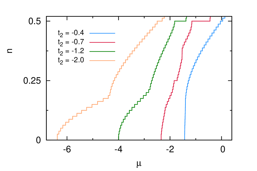
Figure 8: $\mu$-$n$-curve for cuts through phase diagram Fig. 11 for $\delta=1/2$ and (from left to right) $t_{2}=-2.0$, $-1.2$, $-1.0$ and $-0.7$.

In Fig. 7 we show the phase diagram in the $\mu$-$t_{2}$-plane. Consistent with the proceeding section we do not find the emergence of a CSF phase at small values of $\delta$ in the dilute limit. However, at larger fillings the system enters an extensive CSF region. Apart from this, other interesting features appear in the phase diagram which we discuss below.

The phase transition points can be best read from the $\mu$-$n$-diagrams of finite systems which is shown in Fig. 8 for different values of $t_{2}$. At the transition points between the single component superfluid phases such as the SF and the SF_π/2 phases and the CSF or 2SF phases the $\mu$-$n$-curve exhibits a sharp kink. In order to distinguish the 2SF and CSF phases we use the the chirality order parameter and the central charge as discussed before. We observe the SF_π/2-CSF transition for a critical density $n_{c}\approx 0.18$ (for $t_{2}=-2$) which is consistent with $n_{c}=1/6$ that is already obtained in the decoupled chain limit using Eq. (12).

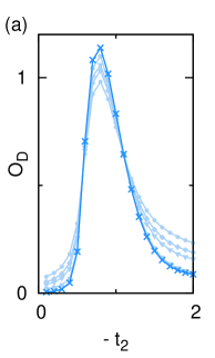
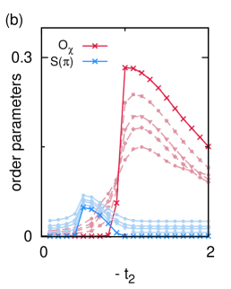
Figure 9: Order parameters for different cuts through the phase diagram for (a) $n=1/2$ and (b) $n=1/4$. The curves in lighter shadings show the finite-size results for $L=20$ (circle), $40$ (diamond), $80$ (triangle) and $160$ (box) sites - cross-symbols depict the extrapolation to the thermodynamic limit using a higher order polynomial.

The $\mu$-$n$-curves of Fig. 8 show a series of plateaus at certain commensurate fillings, $n=1/4$ and $n=1/2$. These correspond to the gaped insulating phases, a density wave(DW) phase(at $n=1/4$) and a dimerized(D) phase ($n=1/2$), which are stabilized due to frustration and asymmetry of the model. As discussed in Ref. Greschner et al. (2013) at the Lifshitz transition, the band curvature vanishes locally as the minimum becomes quartic. Hence, as the effective mass diverges we may expect the pinning of particles at weak interaction strengths resulting into the emergence of gaped phases. In Fig. 7 we show the approximate extent of the plateau regions bounded by the dashed curves which are calculated for several finite system sizes and then extrapolated to the thermodynamic limit by means of a higher order polynomial. For the case of hardcore bosons, the presence of a D phase at half filling $n=1/2$ (for zero magnetic field in the case of the corresponding spin-1/2 model) has been discussed extensively Okamoto and Nomura (1992); Hikihara et al. (2001). Following Okamoto and Nomura Okamoto and Nomura (1992) we may extract the phase transition points between the SF₀ and the D phase by means of a level crossing analysis. To further characterize the D phase we compute the dimer-dimer order parameter as

$$O_{D}=\frac{1}{L}\sum_{i}(-1)^{i}B_{i},$$ (24)

where $B_{i}=\langle b_{i}(b_{i+1}^{\dagger}+b_{i-1}^{\dagger})\rangle$ is the bond energy. In Fig. 9 (a) we show the behaviour of $O_{D}$ at half filling as a function of $t_{2}$ for different system sizes $L=20,~{}40,~{}80,~{}160$ along with the extrapolated curve in the thermodynamic limit.

Interestingly, for the RRT model we also find an emerging density wave (DW) phase at quarter filling $n=1/4$ close to the Lifshitz line. The emerging DW order can be seen as a peak in the density structure factor

$$S(k)=\frac{1}{L^{2}}\sum_{i,j}{e^{ik(i-j)}}\langle{n_{i}n_{j}}\rangle,$$ (25)

where $\langle{n_{i}n_{j}}\rangle$ is the density-density correlation between sites $i$ and $j$. In Fig. 9 (b) we plot the values of $S(k=\pi)$(blue symbols) and the chirality $O_{\chi}$(red symbols) as a function of $t_{2}/t_{1}$ for different lengths and also in the thermodynamic limit at $n=1/4$. This clearly shows the presence of the DW phase for some intermediate range of $t_{2}$ and the system possesses finite chirality for larger values of $t_{2}$ where a CSF phase is found. Note that the chirality becomes finite abruptly with the vanishing of the DW-order parameter as we enter the CSF phase.

III.3 Symmetric zig-zag model

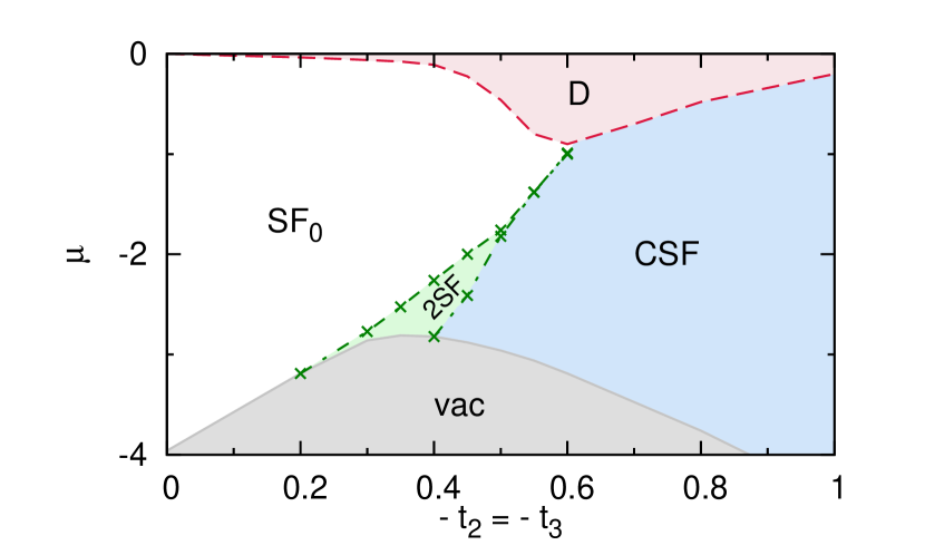
Figure 10: Phase diagram for hardcore bosons in a symmetric frustrated zig-zag ladder ($\delta=1$) in the $t_{2}=t_{3}$ and $\mu$ plane.

Contrary to the previously discussed case, for the symmetric zig-zag model ($\delta=1$), the dispersion relation is doubly degenerate for every $-t_{2}>1/4$. For completeness we depict the corresponding phase diagram in Fig. 10. Here, we find an extended CSF phase for any filling as $-t_{2}$ is large enough. For small densities, close to the Lifsitz transition the interesting interplay between the 2SF and CSF phases is observed. The transition point from the low density description is consistent with the numerical simulations. Due to the symmetry of the model the DW phase at quarter filling is absent. However, there exists a D phase at $n=1/2$ as a result of frustration.

IV The $\pi$-$0$ case

Let us now turn to the anti-symmetric case when $\delta<0$, i.e. a model with a $\pi$ flux through every second plaquette. Here we analyze this model along the line discussed above and obtain the complete phase diagram as shown in Fig. 11 for $\delta=-0.5$. The phase diagram is obtained by analyzing the plateaus in the $\mu-n$ plot (Fig. 12) and the order parameters as done in the previous case. Fig. 12 shows the emergence of plateaus only at $n=1/4$ which corresponds the the DW phase. This DW phase is denoted by the region bounded by the dashed curve in Fig. 11. Interestingly a gapped phase at half filling is absent in this case. The extent of the DW phase is drastically enhanced compared to the case of a $\pi$-$\pi$-flux. In particular, for large values of $-t_{2}$ we still observe a finite gap after extrapolation of our numerical data to the thermodynamic limit. The grey region bounded by the continuous line is the empty state.

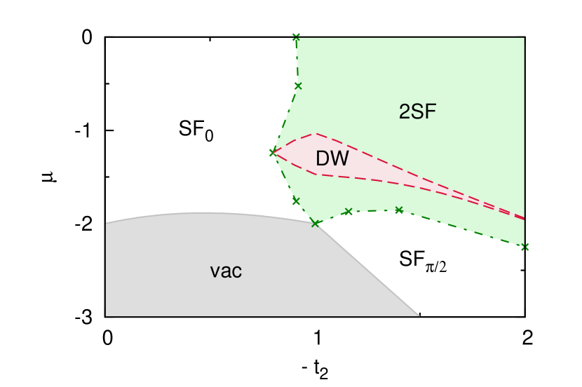
Figure 11: Phase diagram of the $\pi$-$0$ RRT model with $\delta=-1/2$.

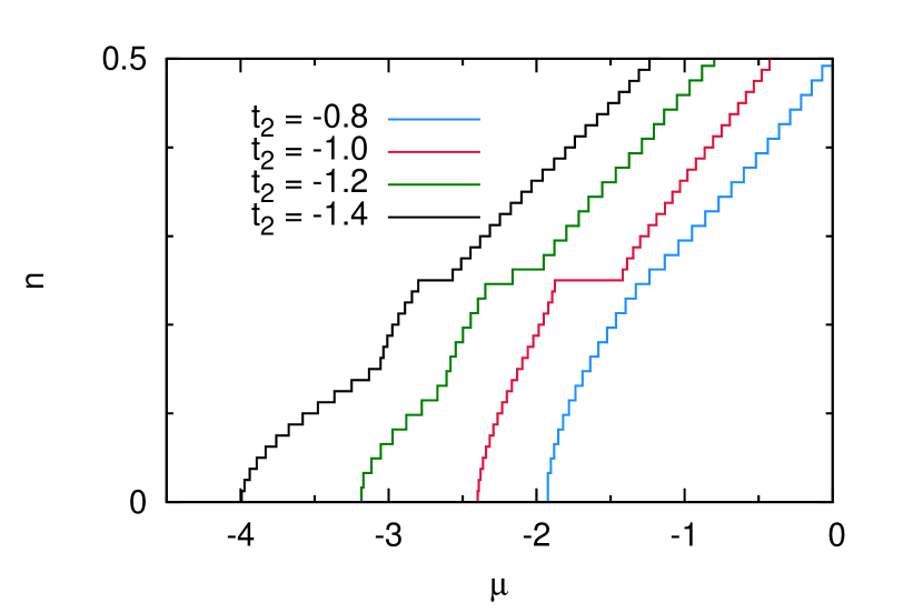
Figure 12: $n$-$\mu$-curve for cuts through phase diagram of Fig. 11 for $\delta=-1/2$ and $t_{2}=-1.4$, $-1.2$, $-1.0$ and $-0.8$(from left to right).

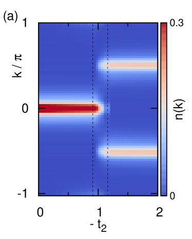
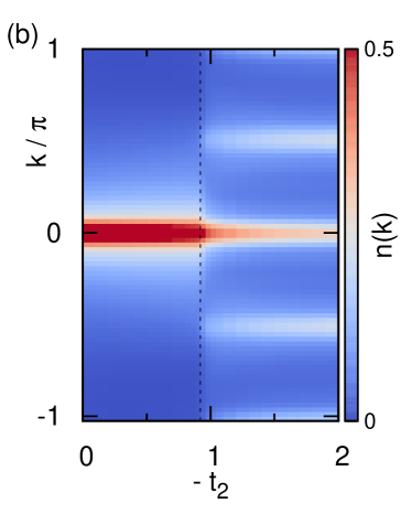
Figure 13: Momentum distributions for filling $n=1/8$ and $3/8$ which corresponds to two cuts in the phase diagram of Fig. 11.

As discussed in Sec. (II), there should not exist a CSF phase in this scenario for weakly coupled chains, which we find to remain valid also for a finite inter-leg hopping. We confirm this using our DMRG calculation and indeed, we see a broad region of the 2SF phase around the gapped DW phase marked by the dashed-cross boundary. The transition to the 2SF phase is characterized by a series of kinks in the $\mu$-$n$-curve (see Fig. 11).

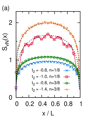
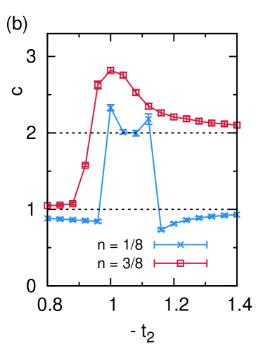
Figure 14: Entanglement scaling for the $\delta<0$ RRT model using the same parameters as in Fig. 4 (DMRG data, $L=201$ sites, filling $n=0.1$). (a) Entanglement entropy $S_{vN}(x)$ for different bi-partitions of the system $x$ for various values of $\delta$. The black dashed lines depict a fit to Eq. (23). (b) The extracted central charge $c$ from the fitting procedure.

The SF₀ and SF_π/2 phases are best understood by looking at the momentum distribution function $n(k)$ as plotted in Fig.13. We plot $n(k)$ for two cuts through the phase diagram of Fig.11 along the X-axis which correspond to two different fillings $n=1/8$ and $n=3/8$ in Fig.13(a) and Fig.13(b) respectively. For the cut along $n=1/8$, the momentum distribution exhibits one peak at $k_{0}$, then three peaks and in the end two peaks at $k=\pm\pi/2$ as a function of $t_{2}$. While the SF_π/2 phase is characterized by peaks at $k=\pm\pi/2$, which are equivalent, in the 2SF phase region we find multi-peak structure with peaks at $k=0$ and $\pm\pi/2$. This means the system goes from the SF to the SF_π/2 phase and then to the 2SF phase. In the case of $n=3/8$, there is a single transition from the SF to the 2SF phase as can be seen from Fig.13(b). The phase transitions between these superfluid phases are marked by the vertical dashed lines in Fig. 13. We also compute the central charge $c$ following the analysis done in the previous section and show that the numerical estimation of the central charge is consistent with $c=1$ in the SF₀ and SF_π/2 phases where as $c=2$ in the 2SF regions(see Fig. 14).

V The sawtooth chain

In the end we analyze the very special case of the RRT model which is known as the sawtooth chain. As stated in the introduction, for the sawtooth case ($\delta=0$) the lowest band becomes exactly flat at the special value of $t_{2}=-1/\sqrt{2}$ (see Fig. 2(c)).

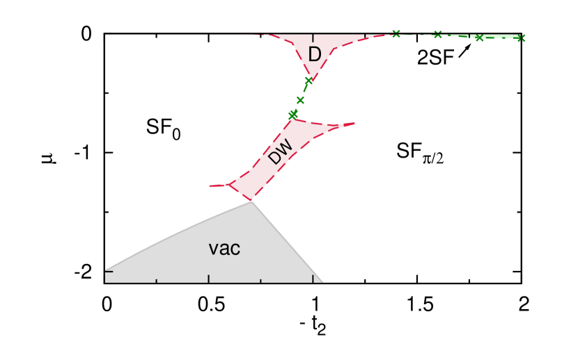
Figure 15: The phase diagram for the sawtooth ladder model for hardcore bosons.

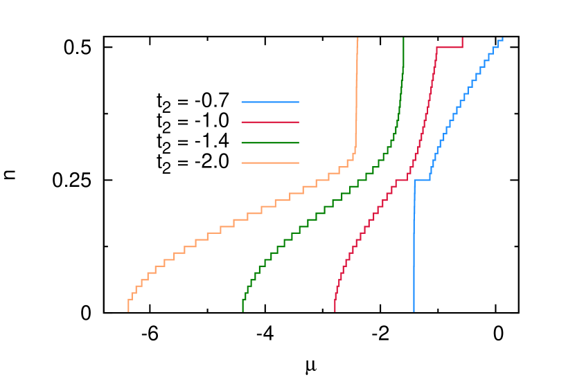
Figure 16: $\mu$-$n$-curve for $t_{2}=-0.7$, $-1.0$, $-1.4$ and $-2.0$ (right to left) for the sawtooth model.

Here we analyze the sawtooth model for the hardcore bosons case and obtain the interesting ground state phase diagram which is shown in Fig. 15 . Examples of the equation of state from which the main results can be deduced are shown in Fig. 16.

The presence of the flat band leads, as for the Lifshitz transitions, to an enhancement of correlations. As a result we find an extensive D and DW phase around $t_{2}=-1/\sqrt{2}$ which are bounded by the dashed curves in Fig. 15 at $n=1/2$ and $n=1/4$ respectively. The presence of the flat-band also leads to macroscopically large jumps in density in the $\mu-n$ curve for fillings below $n=1/4$. The transition between the SF and SF_π/2 phase is apparently direct, possibly of first order. For the hardcore case we do not observe an emerging supersolid phase like the softcore case discussed in Ref. Mishra et al. (2015b), however, we find a 2SF phase for large fillings and $-t_{2}\gtrsim 1.4$. As seen in Fig. 16 it is characterized by a sharp increase in the density which indicates a very large but finite compressibility.

VI Summary

In summary in this paper we have studied the ground-state physics of a very generic zig-zag ladder model, with asymmetric hopping strengths on the two legs. The interplay between this asymmetry and the interactions of the bosonic particles gives rise to various phenomena and quantum phases including the 2SF and the CSF phases and different single component SF phases. At certain commensurate fillings density wave and dimerized phases can be observed. While for the symmetric case chiral phases dominate the grand canonical phase diagram, the asymmetry tends to stabilize the 2SF phases.

In state of the art ultra-cold atom experiments the RRT models should in a natural way emerge from the attempts to study the symmetric zig-zag ladder models. For example one may realize a zig-zag model by means of superlattice techniques on triangular lattices in combination with lattice shaking Struck et al. (2012); Greschner et al. (2013). A slight misalignment of superlattice and the triangular lattice might typically lead to the tunneling asymmetry described here. Also one might adapt synthetic dimension approaches as recently proposed in Ref.Anisimovas et al. (2016), where the requirement of a state-dependent lattice also may be naturally exploited to generalize to RRT-type models.