Testing massive star evolution, star formation history, and feedback at low metallicity

Stars that start their lives with spectral types O and early B are the progenitors of core-collapse supernovae, long gamma-ray bursts, neutron stars, and black holes. These massive stars are the primary sources of stellar feedback in star-forming galaxies. At low metallicities, the properties of massive stars and their evolution are not yet fully explored. Here we report a spectroscopic study of 320 massive stars of spectral types O (23 stars) and B (297 stars) in the Wing of the Small Magellanic Cloud (SMC). The spectra, which we obtained with the ESO Very Large Telescope, were analyzed using state-of-the-art stellar atmosphere models, and the stellar parameters were determined. We find that the stellar winds of our sample stars are generally much weaker than theoretically expected. The stellar rotation rates show broad, tentatively bi-modal distributions. The upper Hertzsprung-Russell diagram (HRD) is well populated by the stars of our sample from a specific field in the SMC Wing. A few very luminous O stars are found close to the main sequence, while all other, slightly evolved stars obey a strict luminosity limit. Considering additional massive stars in evolved stages, with published parameters and located all over the SMC, essentially confirms this picture. The comparison with single-star evolutionary tracks suggests a dichotomy in the fate of massive stars in the SMC. Only stars with an initial mass below $\sim 30\,M_{\odot}$ seem to evolve from the main sequence to the cool side of the HRD to become a red supergiant and to explode as type II-P supernova. In contrast, stars with initially more than $\sim 30\,M_{\odot}$ appear to stay always hot and might evolve quasi chemically homogeneously, finally collapsing to relatively massive black holes. However, we find no indication that chemical mixing is correlated with rapid rotation.

We measured the key parameters of stellar feedback and established the links between the rates of star formation and supernovae. Our study demonstrates that in metal-poor environments stellar feedback is dominated by core-collapse supernovae in combination with winds and ionizing radiation supplied by a few of the most massive stars. We found indications of the stochastic mode of massive star formation, where the resulting stellar population is fully capable of producing large-scale structures such as the supergiant shell SMC-SGS 1 in the Wing. The low level of feedback in metal-poor stellar populations allows star formation episodes to persist over long timescales.

1 Introduction

Massive stars ($M_{\rm init}\gtrsim 8\,M_{\odot}$) are cosmic engines that play a pivotal role in the physical and chemical evolution of the interstellar medium (ISM) and galaxies via UV radiation, stellar winds, and supernovae (SNe). These stars are among the main sources of reionization of the universe (Barkana 2006). Massive stars are the progenitors of neutron stars and black holes, formed by their core-collapse. Detection of gravitational waves from coalescing black holes further highlighted a need for better understanding of massive stars, especially at low metallicity.

The evolution of a star is mainly decided by its mass, mass-loss history, composition, rotation rate, and binary status. Mass-loss rates ($\dot{M}$) derived empirically are often lower compared to standard prescriptions, especially for low-luminosity OB stars (‘weak wind stars’, Bouret et al. 2003; Martins et al. 2005; Marcolino et al. 2009). The variation of $\dot{M}$ with evolutionary phase and metallicity is still under debate. Especially at highest masses, the evolution of massive stars at low metallicity and their remnant mass at collapse depends critically on the mass loss by winds and eruptions. Stellar evolution models predict rotationally induced chemical mixing in massive main sequence stars and homogeneous evolution channels, predominantly at low metallicity. The presence of a companion can also alter the evolutionary paths (Sana et al. 2012).

The quantitative spectroscopy of massive stars in metal-poor environments is a key to understand their properties, evolution, and feedback in detail. Up to now, the largest spectroscopically analyzed samples refer to the Large Magellanic Cloud (LMC) with metallicity $Z\sim 0.5\,Z_{\odot}$ (Schneider et al. 2018; Ramachandran et al. 2018b). In this paper, we analyze 320 OB stars in the Small Magellanic Cloud (SMC), significantly enlarging the previous studies (Hunter et al. 2008a; Bouret et al. 2013; Castro et al. 2018). Our sample stars belong to the Wing of the SMC, which is the nearest (DM =18.7 mag) (Cignoni et al. 2009) low density (Stanimirovic et al. 2000) and low reddening region at low metallicity. The chemical composition of B stars (C, N, O, Mg, Si and Fe ) obtained by Hunter et al. (2007) and Trundle et al. (2007) compared to solar values (Asplund et al. 2009) suggest the metallicity of SMC to be $\sim 1/7\,Z_{\odot}$. The properties of the Wing match with the typical conditions for low-metallicity dwarf irregular galaxies, which are the most common among star-forming galaxies (Gallagher et al. 1984).

Among the spectacular manifestations of massive star feedback are the large-scale structures in the ISM, such as the H$\alpha$ “supergiant shell” (SGS) in the SMC (SMC-SGS 1, Meaburn 1980), which contains the majority of our sample stars (Fig. 1). It has a closed ring-like morphology (r $\sim 300$ pc ) with a bright rim in the southeast. It is associated with a H i supershell, which shows a central radial velocity of 173 km s^-1 and expansion velocity of $\sim 10$ km s^-1 (Stanimirovic et al. 1999; Fulmer et al. 2019 submitted). However, the formation mechanism of such large structures is still a subject of debate. One source responsible for the huge amount of energy needed for their formation could be the combined effect of ionizing radiation and winds from young clusters or OB associations and SN explosions. Alternative mechanisms include the distortion of the ISM by $\gamma$-ray bursts (Efremov et al. 1999), collisions of high-velocity clouds (HVCs) (Tenorio-Tagle 1981; Tenorio-Tagle et al. 1986), stochastic star formation propagation (Seiden et al. 1979; Matteucci & Chiosi 1983; Harris & Zaritsky 2008), and the turbulent nature of the ISM (Elmegreen 1997). Quantitative feedback studies are necessary to unveil which of the possible mechanisms plays a key role.

The nebular complexes of the region were first identified by Davies et al. (1976) and classified into eight different emission regions DEM 160-167. Three H ii regions, N 88, N 89, and N 90, are located in the rim of the shell (see Fig. 1). A well-studied and prominent site of star formation in the SMC-SGS 1 is the group of young clusters NGC 602. The main cluster NGC 602a and the adjacent cluster NGC 602b are immersed in the emission nebula N 90, while NGC 602c is located in the northeast (Westerlund 1964). The cluster hosts few of the most massive stars in the SMC , including a rare pre-SN star of WO type (Sk 188) in NGC 602c and an early-type O3 star (Sk 183) in NGC 602a (Evans et al. 2012). Many of the OB stars within the SGS do not appear to be bound to any of the clusters and it was suggested that they related to the same triggering event (McCumber et al. 2005).

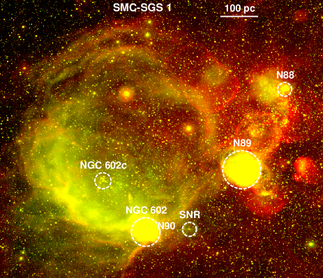
Figure 1: Supergiant shell SMC-SGS1 in the Wing of the SMC. The H ii regions (N 88,89, and 90), clusters (NGC 602 and NGC 602c), and the supernova remnant (SNR) in the region are indicated on the color composite (H$\alpha$, [O iii]) image, taken from the Magellanic Cloud Emission-Line Survey (MCELS, Winkler et al. 2005).

The quantitative spectroscopy of OB star populations in the SMC allows us to test massive star evolution, their feedback, and star formation in low-metallicity galaxies. Through the analyses of OB stars using sophisticated model atmospheres, we provide the stellar and wind parameters of the individual stars and their energy feedback. The spectroscopic observations and data reduction are presented in Sect. 2. In Sect. 3, we quantitatively analyze the OB star spectra using the Potsdam Wolf-Rayet (PoWR) model atmospheres. We present the main results and discussions in Sect. 5 to Sect. 8. The final Sect. 9 provides a summary and general conclusions. The Appendices encompass additional data, figures and tables.

2 Observations and data reduction

We obtained the optical spectra of the OB stars associated with SMC-SGS 1 on 2010 October 24-26 with the Fiber Large Array Multi-Element Spectrograph (FLAMES) on ESO’s Very Large Telescope (VLT). Using the Medusa-fiber mode of FLAMES (Pasquini et al. 2002), spectra on 132 targets were simultaneously recorded, where each fiber has an aperture of $1.2\arcsec$ on the sky. Three of the standard settings of the Giraffe spectrograph LR02 (resolving power $R$ = 6000, 3960–4567 Å), LR03 ($R$ = 7500, 4501–5071 Å), and HR15N ($R$ = 19200, 6442–6817 Å) were used for this survey. The higher resolution spectra of H$\alpha$ serve for the determination of the wind parameters and to distinguish nebular emission from the stellar component.

Our observation constraint was a magnitude cut of $V\leq 17$ mag (based on Massey 2002), corresponding to unreddened O and early B-type stars at the distance of the SMC. We could not apply further constraints since no other photometry data were available at the time of observation. The exposure time for each pointing is 1800 s in all three spectrograph settings. We took three to six exposures for each target to get an S/N$>50$.

The ESO Common Pipeline Library (CPL) FLAMES reduction routines were executed for the standard data processing stages, i.e., bias subtraction, fiber location, summed extractions, division by a normalized flat-field, and wavelength calibration. All these spectra were then corrected to the heliocentric frame. A number of fibers was placed on the sky background. Each sky fiber was inspected and the contaminated sky fibers were rejected prior to the creation of a median sky spectrum for each observation. This median sky spectrum was then subtracted from all stellar spectra. However, because of the prominent nebular regions in the shell, the majority of the spectra are still contaminated by nebular emission lines such as H$\alpha$, [O iii], [N ii], and [S ii].

To clean the extracted spectra of cosmic rays, we calculated the ratio of the two exposures for each spectrum. Since these exposures were consecutive, we assumed that any unexpected and significant deviations in the ratio are indicative of a cosmic ray. The pixels identified as suspect were rejected, then replaced with the value from the sister exposure, appropriately scaled by the ratio of the surrounding pixel.

The obtained spectra are not flux-calibrated. The spectra were rectified by fitting the stellar continuum with a cubic spline function. For each star, the LR02 and LR03 spectra were merged to form the medium resolution blue spectrum from 3960 to 5071 Å. We obtained spectra of 543 individual stars. Since we only applied a V magnitude cutoff, the sample also contains late-type stars, foreground stars, and objects with poor S/N. By inspection of the blue spectra, we eliminated them from our final catalog. We are only interested in hot blue stars in this study. The final catalog contains 320 OB stars. The survey covers a large part of the SGS with a total area of 0.28 kpc². We adopt a naming convention for all the objects in the survey starting with SMCSGS-FS (SMC supergiant shell FLAMES Survey) and a number in ascending order with their right ascension (1–320). The full catalog of the survey targets are available in Table B.1 in electronic form at the CDS with their names, positions, and spectral types.

Flux-calibrated UV spectra are available in the Mikulski Archive for Space Telescopes (MAST) for nine OB stars of our sample. All these stars (SMCSGS-FS 96, 216, 231, 284, 287, 288, 292, 298, and 310) have an International Ultraviolet Explorer (IUE) spectrum in the wavelength range 1150–2000 Å. For SMCSGS-FS 310, there exists an HST/Space Telescope Imaging Spectrograph (STIS) spectrum, a far-UV Far Ultraviolet Spectroscopic Explorer (FUSE), and a high-resolution Ultraviolet and Visual Echelle Spectrograph (UVES) spectrum. The HST spectrum was taken with the G130M grating in the wavelength range 1135–1429 Å, with an effective resolving power of $R$ = 18000. The FUSE spectrum was taken with a large aperture ($30\arcsec\times 30\arcsec$), and extends over the wavelength range 905–1187 Å. The UVES spectra cover wavelength ranges of 3750–5000 Å, 4600–6600 Å, and 6700–11000 Å  with a resolving power of $R\sim 35000$.

In addition to the spectra, we adopted various photometric data from the VizieR archive, for constructing the spectral energy distributions (SEDs). Ultraviolet and optical ($U,B,V,$ and $I$) photometry was taken from Massey (2002), Zaritsky et al. (2004), Girard et al. (2011), and Zacharias et al. (2012). The infrared magnitudes ($JHK_{s}$ and Spitzer-$IRAC$) of the OB stars are taken from the catalogs Kato et al. (2007), Bonanos et al. (2009), and Cutri et al. (2012).

Spectral classification

We visually compared the blue optical spectra of our sample stars to those of classified stars from Sota et al. (2011, 2014), Walborn et al. (2014), Evans et al. (2015), and McEvoy et al. (2015), while also taking into account the low metallicity of the SMC compared to the Galaxy and the LMC. Detailed descriptions of the subtype classification of OB stars are given in Ramachandran et al. (2018a) and Ramachandran et al. (2018b). The spectral classifications of all stars are tabulated in Table LABEL:table:App_coord.

We identified 23 O stars and 297 B stars in the whole sample based on He i/He ii ionization equilibrium. In O stars, the He i lines get weaker and He ii lines get stronger as going toward the earliest subclasses. So, for the classification of early O subtypes, we used the strength and morphology of the optical nitrogen lines N iii $\lambda\lambda$4634–4642 (hereafter N iii) and N iv $\lambda 4058$ (hereafter N iv) (Mihalas et al. 1972; Walborn et al. 2002). We identified these nitrogen emission lines in four of our sample stars, known as Of stars. The nitrogen emission lines of these stars are weaker than the LMC stars of similar spectral subtype.

The sample contains a very early-type O3 star, SMCSGS-FS 231 (Sk 183), which shows N iv and N iii emission lines in the spectra. Part of our team has studied this star in detail previously (see Evans et al. 2012). We identified another early spectral subtype O6 star, SMCSGS-FS 287, which shows weak N iii emission lines and very strong He ii absorption lines. Two O7 stars (SMCSGS-FS 241 and 292) are present in the sample, where only SMCSGS-FS 292 is identified as an Of star based on very weak N iii emission lines (no available LR03 spectra for SMCSGS-FS 241 to assign this classification). All these three Of stars have a prominent He ii 4686 absorption feature that is stronger than any other He line in the blue-violet spectra. This characteristic represents the Vz luminosity class. Stars of this class are expected to be very young and may be near or on the zero-age main sequence (ZAMS) (Walborn 1973, 2009). However, analysis of O Vz stars in 30 Doradus by Sabín-Sanjulián et al. (2014) revealed that they might be in more evolved phases because of weaker O-star winds in the low-metallicity environment of the LMC compared to the Galaxy.

A peculiar Of supergiant, SMCSGS-FS 310 (Sk 190) is part of the sample. We classified this star as O7.5 based on its strong He ii absorption lines and very weak N iii emission lines. The He i absorption lines are very weak in the blue optical spectrum. The weak He ii 4686 emission wings in the spectrum qualify its Onfp nature. This spectral class was introduced by Walborn (1973) to describe a composite emission + absorption profile at He ii 4686. In this case “f” denotes He ii 4686 and N iii emission, “p” refers to peculiar early-type spectra and the broadened absorption lines due to rapid rotation is indicated with “n” (Walborn 1973; Walborn et al. 2010). Since the He ii 4686 absorption line is negligible or very weak compared to the emission wings, the star might be an Of supergiant. Hence we assigned a spectral type of O7.5 In(f)p to the star. Such evolved stars are not expected to rotate rapidly because of strong mass loss. Walborn et al. (2010) discussed possible reasons for their rapid rotation such as binarity and stellar mergers. These types of stars are also considered as gamma-ray-burst progenitors.

All other 18 O stars are of late subtype O8–9.7. These are mostly main sequence stars since their He ii 4686 absorption line is strong. One of these, SMCSGS-FS 269, is identified to be a Vz luminosity class star. Because of the weak He ii 4686 absorption, SMCSGS-FS 288 is classified as a giant.

We subclassified all sample B stars into B0–9 based on the ionization equilibrium of helium and silicon. The main diagnostics used for early B types (B0–2) are the Si iii $\lambda$4553/ Si iv $\lambda$4089 line ratio and the strength of He ii $\lambda 4686$, He ii $\lambda 4542$, and Mg ii $\lambda 4481$. Approximately two-thirds of the sample are in the early B-star category, as highlighted by the histogram shown in Fig. 2. The spectral subtype with highest number of sample stars is B2. This is because, the sample is not complete in the case of late B stars (B2.5–9). We identified a total of 95 stars later than B2. The main diagnostic lines used to subclassify these late B-type stars are Si ii $\lambda\lambda$4128-4132, He i $\lambda 4144$, He i $\lambda 4471$, and Mg ii $\lambda 4481$.

The main criteria used for determining the luminosity classes of B stars are the width of the Balmer lines and the intensity of the Si iv and Si iii absorption lines (Evans et al. 2015). We identified five B supergiants in the sample, which show rich absorption-line spectra. Among these, four are late B9 supergiants and one is a B2 supergiant. There are also 20 giants / bright giants present in the sample and the rest are main sequence B stars. Ramachandran et al. (2018b) and Evans et al. (2015) provide a detailed description of spectral and luminosity classifications of B stars.

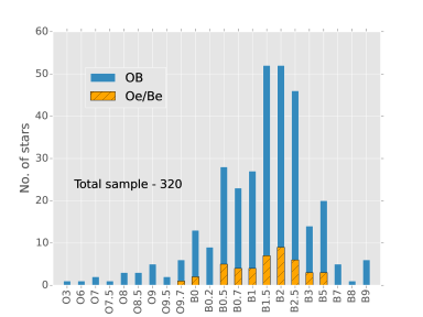
Figure 2: Spectral subtype distribution of all OB stars in our sample. For each spectral subtype, the number of detected Oe/Be stars are represented in orange with black lines.

We identified 44 stars with strong emission lines among the whole sample. The optical spectra of these non-supergiant stars exhibit broad Balmer emission lines, especially H$\alpha$. These are characteristic features of Be (or Oe) stars, which emerge from their circumstellar decretion disk. The high-resolution H$\alpha$ observations (HR15N) helped us to distinguish disk emission profiles. In some cases, we observed a double-horn profile in H$\alpha$ and H$\beta$. Some spectra are contaminated by nebular emission.

The fraction of Be stars in the sample is about 15%. This is slightly higher than that of our LMC sample described in Ramachandran et al. (2018b). This fraction is just a lower limit since we have only single epoch spectroscopic observations of our sample stars. We might have missed a fraction of Be stars owing to their transient nature and variability in the emission line profiles (about one-third to one-half, McSwain et al. 2008). Among this Be sample, 15 stars are identified as giants or bright giants, while the rest are dwarfs. These Be stars have spectral subtypes ranging from B0 to B5 (see Fig. 2). Interestingly, 15 out of 25 B-type giants are Be stars.

The statistics of spectral subtypes of all investigated OB stars is shown in Fig. 2. Emission line stars in each subtype are also illustrated. We can see a gradual increase in the number of stars with spectral subtypes starting from O3, until B2. Stars with spectral subtype B2 are the most common, while this spectral class also encompasses more Be stars than any other. The number of stars declines toward late B subtypes most probably because of our brightness limit.

3 Quantitative analysis

We performed the spectral analysis of all 320 sample OB stars in SMC-SGS 1 using the PoWR model atmosphere code. By fitting the model spectra to the observational data, we derive stellar and wind parameters of the individual OB stars.

3.1 Models

PoWR is a state-of-the-art stellar atmosphere code suitable for the spectroscopic analysis of any hot stars with and without winds, across a broad range of metallicities (Hainich et al. 2014, 2015; Oskinova et al. 2011). The PoWR models have already been used to analyze the complete sample of Wolf-Rayet (WR) stars and binaries in the SMC (Hainich et al. 2015; Shenar et al. 2016). The PoWR code solves the radiative transfer equation for a spherically expanding atmosphere and the statistical equilibrium equations simultaneously under the constraint of energy conservation. Stellar parameters were determined iteratively. Details of the PoWR code are described in Gräfener et al. (2002), Hamann & Gräfener (2004), Sander et al. (2015), and Todt et al. (2015).

A PoWR model is specified by the star’s luminosity $L$, stellar temperature $T_{\ast}$, surface gravity $g_{\ast}$, and mass-loss rate $\dot{M}$ as the main parameters. The stellar temperature relates to $R_{\ast}$ and $L$ via the Stefan-Boltzmann law $L=4\pi\sigma_{\mathrm{SB}}\,R_{\ast}^{2}\,T_{\ast}^{4}$. In this case the “stellar temperature” $T_{\ast}$ is the effective temperature $T_{\mathrm{eff}}$ corresponding to the stellar radius $R_{\ast}$. We place the latter at the Rosseland continuum optical depth of 20. In the case of our program stars, the winds are optically thin and the differences between $T_{\ast}$ and $T_{\mathrm{eff}}$ ($\tau=2/3$) are negligible.

In the subsonic region of the stellar atmosphere, a velocity field is defined such that a hydrostatic density stratification is approached (Sander et al. 2015). In the supersonic region, the prespecified wind velocity field $\varv(r)$ is assumed to follow the so-called $\beta$ -law (Castor et al. 1975) In this work, we adopt $\beta$=0.8, which is a typical value for O-type stars (Kudritzki et al. 1989).

In the non-LTE iteration in the co-moving frame, the line opacity and emissivity profiles are Gaussians with a constant Doppler width $\varv_{\mathrm{Dop}}$. We set this parameter to 30 km s^-1 for our OB sample. In the formal integral for the calculation of the emergent spectrum, the Doppler velocity is split into the depth-dependent thermal velocity and a “microturbulence velocity” $\xi(r)$. The pressure broadening is also taken into account by means of microturbulent velocity. We adopt $\xi(r)=\rm max(\xi_{min},\,0.1\varv(\emph{r}))$ for OB models, where $\rm\xi_{min}=20$ km s^-1 (Shenar et al. 2016). For main-sequence B stars, $\rm\xi_{min}$ can be low as $5$ km s^-1 (Hunter et al. 2008a; Dufton et al. 2006). By constructing some models with lower microturbulence velocities, we found that this effect is within the uncertainty limits of our grid parameters.

Optically thin inhomogeneities in the model iterations are described by the “clumping factor” $D$ by which the density in the clumps is enhanced compared to a homogeneous wind of the same $\dot{M}$ (Hamann & Koesterke 1998). For all the OB stars in our study, we account for depth-dependent clumping assuming that clumping begins at the sonic point, increases outward, and reaches a density contrast of $D=10$ at a radius of $R_{\mathrm{D}}=\,10\,R_{\ast}$ (Runacres & Owocki 2002). We note that the empirical mass-loss rates when derived from H$\alpha$ emission scale with $D^{-1/2}$, since this line is mainly fed via recombination.

The models are calculated using complex atomic data of H, He, C, N, O, Si, Mg, S, P, and Fe group elements. The iron group elements are treated with the so-called superlevel approach as described in Gräfener et al. (2002). We adopt the following chemical abundance based on Trundle et al. (2007) : $X_{\rm H}=0.7375$, $X_{\rm C}=2.1\times 10^{-4}$ , $X_{\rm N}=3.26\times 10^{-5}$, $X_{\rm O}=1.13\times 10^{-3}$, $X_{\rm Si}=1.3\times 10^{-4}$, $X_{\rm Mg}=9.9\times 10^{-5}$, $X_{\rm S}=4.42\times 10^{-5}$, $X_{\rm P}=8.32\times 10^{-7}$, and $X_{\rm Fe}=3.52\times 10^{-4}$.

3.2 Spectral fitting

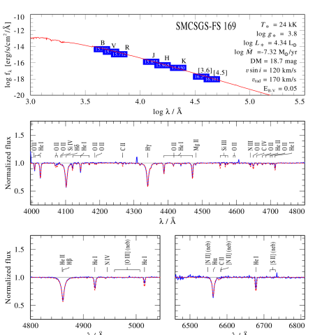
Figure 3: Spectral fit for SMCSGS-FS 169. Top panel: The model SED (red) fitted to the available photometry from optical ($UBV$ and $I$), and infrared ($JHK_{s}$ and $IRAC$ 3.6 & 4.5 $\rm\mu m$) bands (blue boxes). Botton panels: The VLT-FLAMES spectra (blue solid line), overplotted with the PoWR model (red dashed line). The parameters of this best-fit model are given in Table LABEL:table:App_stellarparameters.

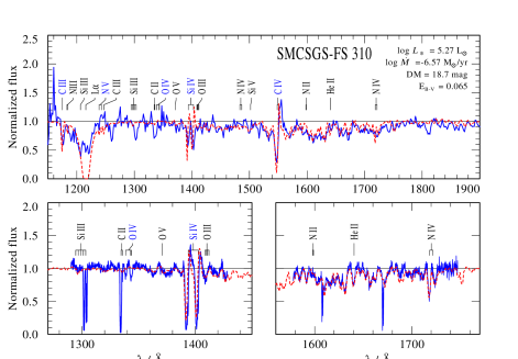
Figure 4: Spectral fit for SMCSGS-FS 310. The panels show the normalized HST (blue solid line), overplotted with the PoWR model (red dashed line). The parameters of this best-fit model are given in Table LABEL:table:App_stellarparameters.

For a systematic spectral analysis, we constructed grids of OB-star model atmospheres for SMC metallicity with the stellar temperature $T_{\ast}$ and the surface gravity $\log\,g_{\ast}$ as main parameters. The grid spans from $T_{\ast}$ = 10 kK to 50 kK with a spacing of 1 kK, and $\log\,g_{\ast}$ = 2.0 to 4.4 [cm s^-2] with a spacing of 0.2 dex. For a given value of ($T_{\ast}$,$\log\,g_{\ast}$), the stellar mass $M$ and luminosity $L$ are chosen according to the evolutionary tracks calculated by Brott et al. (2011). While the chemical composition is kept constant within the model grid, we also calculate specific models with adjusted C, N, O, Si abundances, when necessary. The SMC OB star grid is also available online. More details of the PoWR model grids for OB stars are given in Hainich et al. (2018).

For all the 320 OB stellar spectra in the sample, we determined the best-fitting model by a careful iterative visual comparison of observed spectra with the model. We considered only single-star models for the fits. Our first step was to find the main parameters, i.e., the stellar temperature and surface gravity of the model that best represents the observed spectrum. The primary constraint we used is the helium and silicon ionization balance to determine whether the spectrum represents a very hot O star or cooler B star. For the hottest stars in the sample, we derived the stellar temperature by consistently fitting nitrogen emission lines and He ii lines. In the case of cooler stars (10-20 kK), we determined the temperature by fitting Si ii, Mg ii, and He i lines. For intermediate temperature stars, we used the Si iii to Si iv and He i / He ii line ratios. The precision in the temperature is limited by the grid resolution of $\pm$1 kK. After getting a constraint on the temperature, we measured the surface gravity using the pressure-broadened wings of the Balmer lines. The main diagnostic lines are H$\gamma$ and H$\delta$, since they are less affected by wind as well as disk emission. The typical uncertainty for $\log\,g_{\ast}$ is $\pm$0.2 dex. Since the ionization balance also reacts on $\log\,g_{\ast}$, the temperature might need to readjust accordingly. The uncertainty in $\log\,g_{\ast}$ therefore propagates to the temperature and leads to a total uncertainty of about $\pm$2 kK. As example, the spectra of an O8 star (blue lines) is shown in Fig. 3 overplotted with a model (red lines) with $T_{\ast}=$ 35 kK and $\log\,g_{\ast}=4.2\,[\rm{cm\,s^{-2}}$]. It should be noted that the above method of spectral fitting is not successful in the case of Be stars, since their Balmer absorption lines may be filled by disk emission. Therefore, the uncertainty in the stellar temperature and surface gravity of these stars is relatively high.

After fixing $T_{\ast}$ and log $g_{\ast}$, we determined the wind parameters whenever possible. The mass-loss rate and terminal velocities ($\varv_{\infty}$) can be estimated from the UV P-Cygni profiles. For nine of our sample stars, UV spectra are available. We used the main diagnostic lines C iv $\lambda\lambda$1548–1551 and Si iv $\lambda\lambda$1393–1403 in the HST / IUE range and P v $\lambda\lambda$1118–1128, C iv $\lambda$1169, and C iii $\lambda$1176 in the FUSE range. The typical uncertainties are $\pm$0.2 dex in $\log\dot{M}$ and $\pm$ 100 km s^-1 $\varv_{\infty}$. Since UV spectra are not available for most of the sample stars, we need to constrain $\dot{M}$ and $\varv_{\infty}$ based on optical lines such as H$\alpha$ and He ii $\lambda 4686$. In fact none of the stars in the sample shows wind emission in H$\alpha$ or He ii $\lambda 4686$ (do not confuse with disk emission in Be stars). In these cases, the adopted mass-loss rate is only an upper limit. For stars with no available UV spectra, we estimated the terminal velocities theoretically from the escape velocity $\varv_{\mathrm{esc}}$. For Galactic massive stars with $T_{\ast}\geq$ 21 kK, the ratio $\varv_{\infty}$/$\varv_{\mathrm{esc}}$ is 2.6 and for stars with $T_{\ast}<$ 21 kK the ratio is $\approx$1.3 (Lamers et al. 1995; Kudritzki & Puls 2000). We adopt a scaling for SMC metallicity using the relation, $\varv_{\infty}\,\propto(Z/Z_{\odot})^{q}$, where $q=0.13$ (Leitherer et al. 1992). The UV spectrum of the sample star SMCSGS-FS 310 is shown in Fig. 4. The derived mass-loss rate and $\varv_{\infty}$ from the UV P-Cygni profiles are $\log\dot{M}$ = -6.6 [$M_{\odot}\,\mathrm{yr}^{-1}$] and 550 km s^-1, respectively.

We determined the luminosity $L$ and color excess $E_{\rm B-V}$ of the individual OB stars by fitting the model SED to the photometry (see first panel of Fig. 4). In this case the model flux is diluted with the SMC distance modulus of 18.7 mag. We consistently adjusted the color excess and luminosity of the model’s SED to reproduce the observed data. The typical uncertainty in $\log\,L/L_{\odot}$ is about 0.2 dex. For stars with available flux-calibrated UV spectra (HST, IUE, or FUSE), the uncertainty in the luminosity is only $\approx$0.1 dex in these cases. The color excess of OB stars in the Wing of the SMC is very small, typically 0.05 mag.

Subsequently, we chose a best-fit model for each individual OB star in the sample and overplotted the selected model with the observed spectra (eg. Fig. 3 and Fig. 4). There is a systematic shift between synthetic models and observed spectra owing to the radial velocities of sample stars. We measured the radial velocity of individual stars by fitting a number of absorption line centers of the synthetic spectra to the observation. The primary lines used for these measurements are absorption lines of He i, He ii, and Si iii. The typical uncertainty of $\varv_{\rm rad}$ varies from $\pm$10 to 20 km s^-1.

Finally, we estimated the projected rotation velocity $\varv\,\sin i$ of all OB stars from their line profile shapes. The measurements are based on the Fourier transform (FT) method using the iacob-broad tool (Simón-Díaz & Herrero 2014). The primary lines selected for applying these methods are He i, Si iv and Si iii. The typical uncertainty in $\varv\,\sin i$ is $\sim$ 10%. We convolved our model spectra with measured $\varv\,\sin i$ to account for rotational broadening, which results in a consistent fit with the observations. For example, the model spectra shown in Fig. 3 is convolved with a $\varv\,\sin i$ of 300 km s^-1.

We applied these spectral fitting methods in an iterative manner for individual OB star spectrum. More detailed explanations of the fitting procedure for each parameter is given in Ramachandran et al. (2018b). We also calculated individual models with refined stellar parameters and abundances for each of these stars, when necessary. The fitting procedure continued until no further improvement of the fit was possible. The final best-fit models yield the stellar and wind parameters of all OB stars in our sample.

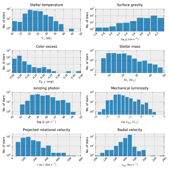
Figure 5: Histograms of stellar temperature, surface gravity, color excess, projected rotational velocity, radial velocity, stellar mass, mass-loss rate, and mechanical luminosity of OB stars in SMC-SGS 1. The bin widths used are 3 kK, 0.18 dex, 0.03 mag, 4 $M_{\odot}$, 0.6 dex, 0.4 dex, 45 km s^-1, and 10 km s^-1, respectively. The number of stars in the y-axis are shown in logarithmic scale.

4 Stellar parameters

The stellar and wind parameters of individual OB stars derived from spectral analysis are given in Table LABEL:table:App_stellarparameters. The PoWR model also gives the rate of hydrogen ionizing photons $Q_{0}$. We calculated the values of mass-loss rate, terminal velocity, and the mechanical luminosity $L_{\mathrm{mec}}\,=\,0.5\,\dot{M}\,\varv_{\infty}^{2}$ produced by the stellar winds only for nine stars with available UV spectra. For the rest of the stars we adopted values from the derived relation of these nine stars. The distribution of some of these derived parameters in the total sample is illustrated in Fig. 5. Since we obtained only single-epoch spectra, we are not able to detect binarity.

The stellar temperature statistics of the sample is shown in the top left panel of Fig. 5. The temperature of our sample stars ranges from 10 kK to 46 kK, with a peak around 20 kK. It has to be emphasized that stars in the low temperature regime are incomplete owing to the observation limit. The earliest type O3 star has the highest stellar temperature of 46 kK. The sample also contains late B supergiants of temperature $\approx 10$ kK. The surface gravities of sample stars are in the range of $10^{2.6}\,\rm{to}\,10^{4.4}\,\rm{cm\,s^{-2}}$, while most of the stars are found at $\log\,g_{\ast}$ of 4.2. This indicates that majority of the sample are young main sequence stars, while only a few percent of the stars are in evolved stages.

The mean color excess of our sample stars is only about $0.05$ mag, which can be mainly attributed to the Galactic foreground. Hence the dust content in the Wing of the SMC is significantly low. Only six percent of the sample shows a color excess higher than 0.1 mag. The star, SMCSGS-FS 45, with highest $E_{\rm B-V}\approx 0.45$ mag is a B supergiant located close to the highly extincted H ii region N 88 (Heydari-Malayeri et al. 1999).

The histogram of the stellar masses given in Fig. 5 ranges from 4 $M_{\odot}$ to 50 $M_{\odot}$. In this figure the stellar mass refers to the spectroscopic mass calculated from $\log\,g_{\ast}$ and $R_{\ast}$ ($g_{\ast}=G\,M_{\ast}\,R_{\ast}^{-2}$). We note that the lowest mass bins are incomplete owing to the observational constraint. Most of the stars in the sample have masses in the range of 10–20  $M_{\odot}$.

The typical ionizing photon flux provided by an OB star in our sample is $10^{45}\,\rm{s^{-1}}$. One O3 star dominates the ionization of the region by releasing photons at a rate of $10^{49}\,\rm{s^{-1}}$.

We also plotted the statistics of the mechanical luminosity $L_{\rm mec}$ released by the stellar winds of our sample stars in Fig. 5. The OB stellar winds in SMC-SGS 1 provide only $L_{\rm mec}<10\,L_{\odot}$ to the surrounding ISM. Most of the stars produce mechanical luminosities a hundred times less than one solar luminosity. This is much lower than the mechanical luminosities of LMC OB stars (Ramachandran et al. 2018a).

4.1 Observed $\varv\sin i$ distributions

We derive the projected rotational velocities ($\varv\sin i$) of our sample stars from their optical line profiles. The $\varv\sin i$ distribution shows a main peak at $\sim$120 km s^-1, and the tail of the distribution extends to high rotational velocities up to 550 km s^-1. The fastest rotator in the sample is a Be star SMCSGS-FS 283, which has $\varv\sin i\approx 550$ km s^-1. We identified 20 very rapidly rotating stars with $\varv\sin i>300$ km s^-1, which constitute 6% of the whole sample. This is double compared to that of our LMC (Ramachandran et al. 2018b). Among these rapid rotators, 12 stars have Oe/Be characteristics. Moreover, we can see a low but noteworthy peak around 300 km s^-1 , which might be related to the effects of mergers and mass transfer in binary evolution (de Mink et al. 2013, 2014).

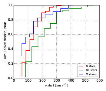
Figure 6: Comparison of CDFs of $\varv\sin i$ between B, Be, and O stars

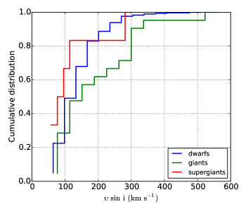
Figure 7: Comparison of $\varv\sin i$ CDFs of dwarfs, giants, and supergiants

For further understanding, we constructed the cumulative distribution functions (CDFs) of the projected rotational velocities of our sample stars. The $\varv\sin i$ CDFs of O, B, and Be stars are compared in Fig. 6. As expected, Be stars exhibit a faster rotation compared to the normal B and O stars in the sample. The mean projected rotational velocities of Be stars in our SMC-SGS 1 sample is $\approx$230 km s^-1, which is significantly higher than the mean $\varv\sin i\approx$140 km s^-1 of normal B stars. Most of the Be stars in this sample rotate close to their critical velocity.

We constructed $\varv\sin i$ CDFs of stars with different luminosity classes as shown in Fig. 7. About 40% of the giants have a $\varv\sin i>200$ km s^-1. On average, they show a higher rotational velocity than unevolved dwarfs or evolved supergiants. Interestingly, 70% of these giants are found to be emission line Be stars. In a study of early-type stars in the SMC, Mokiem et al. (2006) found that very fast and very slow rotators are unevolved with respect to the group of evolved objects. However, in our sample, dwarfs are found to be less fast rotating than giants.

The simulated distribution of projected rotational velocities has a bimodal structure de Mink et al. (2013). Theory predicts that the majority of stars have low to intermediate rotational velocities, whereas nearly one-fourth have rotational velocities in excess of 200 km s^-1. The VLT-FLAMES Tarantula Survey (VFTS) of massive stars in the LMC by Ramírez-Agudelo et al. (2013) and Dufton et al. (2013) also found a bimodal $\varv\sin i$ distribution. In order to check this trend in our sample, we plotted the probability density distribution of OB stars in Fig. 8 (blue solid curve). This reveals a two-component structure with about 26% of stars have $\varv\sin i>200$ km s^-1.

For a comparison, the probability density distribution of $\varv\sin i$ of OB stars for various metallicities (Galaxy, LMC, and SMC) taken from our results and from previous papers are shown in Fig. 8. All these distributions are bimodal. However, there are noticeable differences in the main peak of the distribution (most probable velocity) as well as in the tail of the distribution. At SMC metallicities ($0.14\,Z_{\odot}$), the distribution consists of two broad peaks and the tail of the distribution extends to velocities as high as 500 km s^-1. The $\varv\sin i$ distributions of LMC samples ($0.5\,Z_{\odot}$) have peaks at lower velocities than the the SMC sample. The Galactic samples show main peaks at relatively low velocities ($<50$ km s^-1), the secondary peak is not very pronounced compared to the lower metallicity samples. Obviously, OB stars in the SMC sample have higher rotational velocities. This is a possible consequence of lower SMC metallicity, where the stars are more compact, stellar winds are weaker compared to LMC stars, hence suffer less angular momentum loss and therefore rotate faster (Meynet & Maeder 2002; Massey 2003; Ekström et al. 2008).

The subplot in Fig. 8 (top) shows a linear relationship between the peak of the distribution with the metallicity as given below,

$$\rm{Peak}\,(\varv\sin i)/(\rm{km\,s^{-1}})\simeq-121\times\log\,(Z/Z_{\odot})+22.$$ (1)

The fraction of fast rotating stars above 200 km s^-1 also decreases with increasing metallicity, and can be written in the form,

$$\rm{Fraction}\,(\varv\,\sin\,i>200)\simeq-0.2\times\log\,(Z/Z_{\odot})+0.1.$$ (2)

The OB star sample in the VFTS survey shows a very high fraction of rapidly rotating stars compared to other LMC samples. It should be emphasized that these OB star samples from various papers have different selection criteria, observational biases, and different age distributions, etcetera.

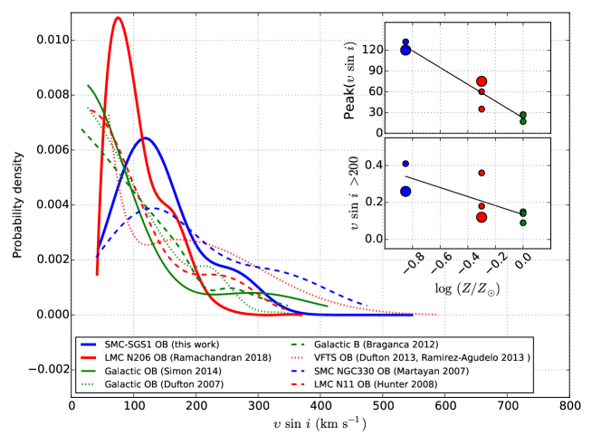
Figure 8: Probability density distribution of projected rotational velocities for metallicities $Z=Z_{\odot}$ (Galactic, green curve), $Z=0.5Z_{\odot}$ (LMC, red curve), and $Z=0.2Z_{\odot}$ (SMC, blue curve). The subplots in the top and bottom show the effect of metallicity with the peak of $\varv\sin i$ distribution / most probable velocity and the fraction of stars with $\varv\sin i$ higher than 200 km s^-1, respectively. The Galactic, LMC and, SMC samples are represented using green, red, and blue dots, respectively. Our SMC (this work) and LMC (Ramachandran et al. 2018b) samples are shown as enlarged dots. See Sect. 4.1 for further information.

4.2 Radial velocity and runaway candidates

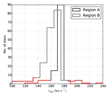
Figure 9: Radial velocity distribution of stars located in region A and B. We used velocity bins of 10 km s^-1 to construct the histogram. The value $|\varv_{\rm rad}|>3\sigma$ is represented by red lines in both histograms.

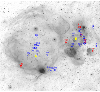
Figure 10: Candidate runaway stars in the sample. The underlying H$\alpha$ image is from the Magellanic Cloud Emission-Line Survey (MCELS, Smith et al. 2005). stars with redshifted and blueshifted velocities are indicated with red and blue circles, respectively. Small circles represent candidate runaway stars with $|\delta\varv_{\rm rad}|>3\sigma$, and large circles for stars with $|\delta\varv_{\rm rad}|>4\sigma$.

The radial velocities in our SMC-SGS 1 sample range from 100 to 240 km s^-1 (see Fig. 5). The peak of the distribution is about $\sim$170 km s^-1, which is close to the central velocity of the associated H i supershell (Staveley-Smith et al. 1997). The ionized gas shell associated with SMC-SGS 1 also has a heliocentric velocity of 173 km s^-1 (Fulmer et al. 2019 submitted). The OB stars in the SMC show a radial velocity gradient, where the velocity distribution of stars in the Wing is more redshifted than in the Bar of the SMC (Evans & Howarth 2008; Lamb et al. 2016). In order to check for the velocity gradient within the SGS, we plotted the radial velocity distribution of stars located near the center of the SGS or close to NGC 602 (region A) and stars located in the western part of the SGS close to N 88 (region B). We can see a small velocity gradient between stars in these two regions (see Fig. 9). Stars in region B exhibit lower radial velocities and higher dispersion than in region A. The region A is within the SGS and has a more sharply peaked velocity distribution. The velocity spread between the stars is similar to the expansion velocity of the present day shell (see Fulmer et al. 2019 submitted, for details about velocity of the shell).

The radial velocities can be used to reveal runaway stars in a region. These are isolated stars or binaries that have escaped from clusters or OB associations as a result of a binary SN (Blaauw 1961) or dynamical ejection (Leonard & Duncan 1990). In order to identify possible runaway candidates, we compared the radial velocity of each star to the mean and standard deviation of all sample stars. Since region A and B have different radial velocity distributions, we decided to check for runaway stars separately in these regions. We defined a velocity threshold of $|\delta\varv_{\rm rad}|>3\sigma$ so that stars with outlying radial velocities are identified as runaway candidates. By excluding these stars, we continued to recalculate the mean velocity and standard deviation, until no more stars with $|\delta\varv_{\rm rad}|>3\sigma$ remain. Using this method, we found 11 and 14 candidate runaway stars in region A and B, respectively. This also includes the HMXB SMCSGS-FS 203 (alias SXP 1062). Their positions are denoted in Fig. 10, while their radial velocities and the deviation from the mean velocity are listed in Table 3 along with their spectral types. Stars with positive and negative radial velocity deviations from the mean are denoted separately in Fig. 10. The mean radial velocity of the OB stars (excluding the runaway candidates) in region A and region B are $169\pm$4 km s^-1 and $163\pm$9 km s^-1, respectively. The velocity dispersions in both regions are very small considering their size. Therefore, we also defined a higher velocity threshold of $|\delta\varv_{\rm rad}|>4\sigma$, which limits the possible runaway stars to four (large circles in Fig. 10). The estimated radial velocity gradient in the region is $\lesssim 3$ km s${}^{-1}\,$deg^-1 along RA and $\lesssim 13$ km s^-1 deg^-1 along Dec.

4.3 Spectral calibrations for OB stars at SMC metallicity

With a sample of 320 OB stars in the Wing of the SMC, our study offers a unique opportunity to calibrate the physical parameters of OB stars. This will be helpful for characterizing massive stars in extragalactic dwarf galaxies. It is not possible to obtain parameters such as temperature and ionizing flux by using optical photometry alone. Using quantitative spectroscopy, we measured these parameters and then calibrated with spectral types. Such studies have been pursued for Galactic (Martins et al. 2005; Repolust et al. 2004), LMC (Ramírez-Agudelo et al. 2017; Mokiem et al. 2007), and SMC (Mokiem et al. 2006; Bouret et al. 2003) massive stars. However, these studies mainly focused on O stars. In this work we extend this up to late B-type stars with a larger sample at SMC metallicity.

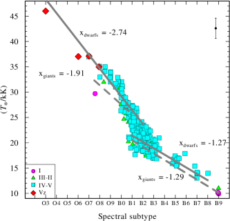
Figure 11: Effective temperature vs. spectral type. The rhombi, squares, triangles, and, circles refer to luminosity classes Vz, V-IV, III-II, and, I, respectively. Typical uncertainties are indicated by the error bar in the top right corner. Gray thick lines represent linear regressions for different subgroups of stars (see text).

Figure 11 shows how the effective temperature correlates with the spectral subtypes. Different luminosity classes are denoted using different colors and symbols as given in the legends. As expected, the evolved stars (III-II and I) systematically possess lower stellar temperatures than dwarfs (Vz and V-IV) of corresponding spectral types. Moreover, we cannot define a single slope for temperature-spectral type relationship from O3 to B9, rather it changes around B1-B2. For stars with spectral type earlier than B1, the relationship is much steeper, and stars with later spectral types than B2 show a shallower relation. For stars with spectral type B1-B2, the temperature determination is more uncertain. The linear regression (see Fig. 11) yields the following relations:

For O3-B1 stars,

$$T_{\ast}[\mathrm{kK}]=\left\{\begin{array}[]{ll}56.60-2.74\times\rm{ST}\hskip 42.67912pt(IV-Vz)\\ 46.61-1.91\times\rm{ST}\hskip 42.67912pt(I-III)\\ \end{array}\right..$$ (3)

For B2-B9 stars,

$$T_{\ast}[\mathrm{kK}]=\left\{\begin{array}[]{ll}35.40-1.27\times\rm{ST}\hskip 42.67912pt(IV-Vz)\\ 34.67-1.29\times\rm{ST}\hskip 42.67912pt(I-III)\\ \end{array}\right..$$ (4)

In this case the spectral subtype is represented by an integer; for example, ST = 3 for an O3 star and ST = 13 for a B3 star. Effective temperature scales of B-type stars in the SMC presented by Trundle et al. (2007) agrees with our calibration within uncertainty limits of $\pm 2$ kK.

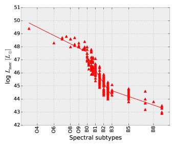
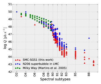
Figure 12: Ionizing photon flux as a function of spectral subtypes (top panel) and the comparison with OB stars at LMC (Ramachandran et al. 2018b) and theoretically predicted values for O stars from Martins et al. (2005).

The PoWR models predict the rate of hydrogen ionizing photons ($Q$) for each individual OB star in our sample (see Table. LABEL:table:App_stellarparameters). We give calibrations of $\log\,Q$ with spectral types in Fig. 12 (top panel). Even though $\log\,Q$ decreases continuously to lower spectral subtypes, we can see breaks near B0 and B3. For O stars and late-type B stars ($\sim$ B3-B9), the slope of the relationship is much shallower than that for early-type B stars (B0-B3). An approximate fit to our data (see top panel in Fig. 12) is

$$\log\,Q\,[\rm{s}^{-1}]=\left\{\begin{array}[]{ll}50.8-0.32\times\rm{ST}\hskip 42.67912pt(O\,stars)\\ 56.9-0.97\times\rm{ST}\hskip 42.67912pt(B0-B3)\\ 47.5-0.22\times\rm{ST}\hskip 42.67912pt(B3-B9)\\ \end{array}\right..$$ (5)

This $\log\,Q$ versus spectral subtype relation shows a similar trend as we found for the N 206 complex in the LMC (Ramachandran et al. 2018b). To check the effect of metallicity on the ionizing photon flux, we plotted the same diagram (see Fig. 12, bottom panel) but include values from Ramachandran et al. (2018b) (LMC stars) and Martins et al. (2005) (Galactic stars). OB stars from the LMC sample (blue circles) also show similar breaks in the diagram. For comparison, theoretically calculated $\log\,Q$ for O stars from Martins et al. (2005) (green squares) are also shown in the plot. Both LMC and Galactic data points match well. However, $\log\,Q$ values of SMC stars for a given spectral subtype are found to be systematically lower compared to the LMC and Galactic samples. Especially, $\log\,Q$ values of the late B stars in LMC and SMC, differ by more than 1 dex.

5 Indications for a dichotomy in massive star evolution independent of rotation

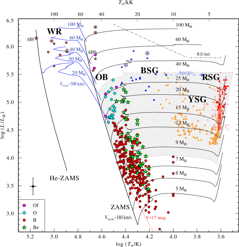
Figure 13: Hertzsprung-Russell diagram for massive stars in the SMC. The OB stars analyzed in this work are represented by different symbols as explained in the legend. The typical error bar is shown in the bottom left corner, above the legend. The brown pentagons represent WR stars (encircled if in binary systems) (Hainich et al. 2015; Shenar et al. 2016), while yellow symbols stand for YSGs (Neugent et al. 2010), blue triangles for BSG (Trundle et al. 2004; Trundle & Lennon 2005) red crosses (Davies et al. 2018) and red triangles (Levesque et al. 2006) for RSGs. The HRD also includes the positions of the only confirmed LBV in the SMC, R40, at different epochs (Kalari et al. 2018). Our OB sample is limited to the SGS in the Wing of the SMC, while as all other samples spread across the whole SMC. Theoretical stellar evolutionary tracks with $\varv_{\rm init}\approx 180\,\rm{km\,s^{-1}}$ are shown by solid lines (Brott et al. 2011; Köhler et al. 2015). The initial masses are indicated above each track. The black tracks show standard evolutionary paths, while the blue tracks with $\varv_{\rm init}\approx 550\,\rm{km\,s^{-1}}$show the tracks of quasi-chemically homogeneously evolving (QCHE) stars. The ZAMS and He-ZAMS are also shown. The shaded gray area indicates the region where, according to standard stellar evolution tracks, stars become RSGs and explode as SNe II-P. However, the more massive star above the gray shaded area do not seem to follow the standard evolutionary tracks. Instead, their location on the HRD is in agreement with QCHE (blue tracks). These stars remain very massive and may undergo core collapse . The figure demonstrates the dichotomy between the SMC stars with initial masses above $\sim 30\,M_{\odot}$ and below, suggesting that the former experience QCHE (blue tracks), while the latter do not.

5.1 Observed Hertzsprung-Russell diagram

Based on the results of our spectral analyses, we construct the Hertzsprung-Russell diagram (Fig. 13) for our sample of 320 OB stars in the SMC. The sample comprises 23 O-type stars, among them four classified as Of, and 297 B-type stars including 44 stars with emission lines (type Be). This gives a well populated upper HRD of hydrogen burning stars with evolutionary masses ($M_{\rm ev}$) in the range of $\sim$5–50 $M_{\odot}$ (see Table B) and covering the parameter space from the ZAMS to the terminal age main sequence (TAMS). The most massive star in our sample is an O3 star (Sk 183), located close to the ZAMS with $M_{\rm ev}\sim 47\,M_{\odot}$ and $\log\,(L/L_{\odot})\sim 5.6$. All other stars have $M_{\rm ev}\lesssim 30\,M_{\odot}$ ($\log\,(L/L_{\odot})\lesssim 5.4$). The sample is complete for $V\lesssim 17$ mag, which translates into a steep limit in the HRD (red dotted line in Fig. 13) due to the temperature dependence of the bolometric correction.

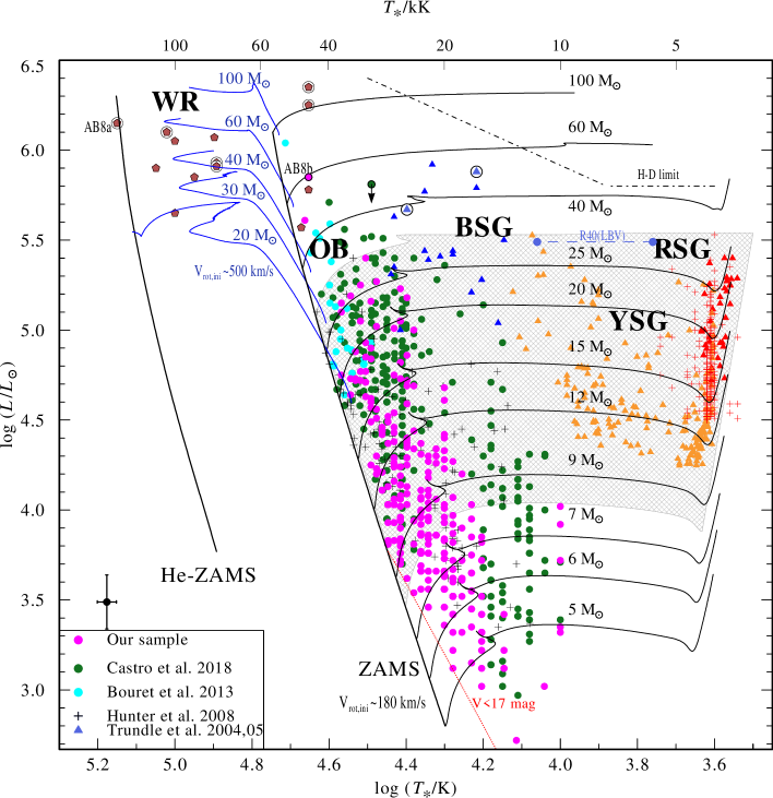
Figure 18: Same as Fig. 13, but including additional OB stars from Castro et al. (2018), Bouret et al. (2013), and Hunter et al. (2008b), bringing the total number of OB stars to about $\sim 800$. While our sample is restricted to the SGS in the Wing of the SMC (see Sect. 7), the other samples spread all over the SMC. The only outstanding star that seems to reside in the void region was obviously confused in the catalog by (Castro et al. 2018); we added a downward arrow because the observed SED definitely indicates $\log L/L_{\odot}<5.2$. The additional samples also support our conclusions on stellar evolution.

To obtain a comprehensive picture of stellar evolution, we incorporate into the HRD samples of red supergiants (RSG), yellow supergiants (YSG), blue supergiants (BSG), luminous blue variables (LBV), and WR stars from previous studies (references are given in the figure caption). While the OB stars of our sample all reside in the supergiant shell SGS1 in the Wing of the SMC (cf. Sect. 7), the other samples are from the whole SMC. The WR (both single and binary) sample is complete for the whole SMC. The shown samples at RSG, YSG, BSG and LBV stages are also complete or nearly complete at high luminosities for this entire galaxy. In the Appendix (Fig. 18) we present a version of the HRD which additionally includes further samples of OB stars from various locations in the body of the SMC, taken from the literature.

All YSG, LBV and RSG stars in the SMC were reported with $\log\,(L/L_{\odot})\lesssim 5.5$. The sample of RSGs in the SMC (complete for $\log\,(L/L_{\odot})>5.0$) has maximum luminosity of $\log\,(L/L_{\odot})\sim 5.5$ (Davies et al. 2018). The region in the HRD above $\log\,(L/L_{\odot})\sim 5.6$ (or $M_{\rm init}\gtrsim 30\,M_{\odot}$) is populated mostly by stars close to the ZAMS or even hotter. Only six luminous BSGs ($\log\,(L/L_{\odot})\gtrsim 5.5$) are seen to the right of ZAMS. These supergiants belong to the brightest blue objects in the SMC, and therefore have $\sim$100% detection probability. Two of these supergiants are reported (Gvaramadze et al. 2011) as runaways (encircled blue triangles in Fig. 13) and, therefore, are most likely products of binary evolution. Another three BSGs show radial velocities that differ by more than $\pm 50\,\rm{km\,s^{-1}}$ from the systemic velocity of the SMC. Such large runaway velocity likely also indicates a binary past. Clearly, further studies on the nature of these BSGs are required.

The empirical HRD (Fig. 13) shows a remarkable pattern: while a few very luminous O stars are found close to the main sequence, all other OB stars as well as the BSGs, YSGs, and RSGs obey strict luminosity limits ($\log L/L_{\odot}<6.0$ for BSGs, and $<5.5$ for the cooler classes). The comparison with single-star evolutionary tracks suggest a dichotomy in the fate of massive stars in the SMC. Only stars with an initial mass below $\sim 30\,M_{\odot}$ seem to evolve from the main sequence to the cool side of the HRD to become a red supergiant. In contrast, stars with initially more than $\sim 30\,M_{\odot}$ appear to stay always hot.

In comparison the tracks for single-star evolution, this would imply that only stars with initially $\lesssim 30\,M_{\odot}$ evolve according to the standard tracks to become red supergiants. For stars with $\gtrsim 30\,M_{\odot}$ such evolution towards the cool side of the HRD is apparently inhibited.

A similar void region in the Galactic HRD is confined by the Humphreys-Davidson (HD) limit, as was empirically established by Humphreys & Davidson (1979) long ago. A couple of stars that are found in the Galaxy, LMC, M31, and M33 which are close to or even slightly beyond the HD limit are considered as unstable stars (LBVs) (e.g. Groh et al. 2013; Martins & Palacios 2013; Urbaneja et al. 2017; Kourniotis et al. 2018; Humphreys et al. 2017, 2016). Our empirical HRD suggests that for the SMC the void region is even more extended than for galaxies with higher metallicity.

Why the SMC stars with initially $\gtrsim 30\,M_{\odot}$ stay at the blue side of the HRD? A tentative explanation is offered by the WR stars. The single WR stars, analyzed by Hainich et al. (2015), all reside between the ZAMS for hydrogen-rich stars and the theoretical He-ZAMS for hypothetical pure-helium stars. Such HRD position can be reached if a star evolves quasi chemically homogeneously, i.e. with efficient internal mixing, as demonstrated by the corresponding tracks in Fig. 13.

All single WR stars in the SMC are hydrogen depleted, but not free of hydrogen. In contrast, WN stars (i.e. WR stars of the nitrogen sequence) in the Galaxy or LMC either reside at the cool side of the ZAMS if showing some hydrogen, or on the hot side of the ZAMS if hydrogen-free. Remarkably, all WR stars in the SMC are very luminous ($\log L/L_{\odot}\gtrsim 5.6$). There are no WR stars with lower luminosities, in contrast to the LMC and the Galaxy (Hainich et al. 2014; Hamann et al. 2006). Considered as a whole, in the SMC the population of single WR stars is strikingly different from higher metallicity environments.

Hence, the large void in the upper HRD, i.e. the absence of any cool stars at high luminosity, together with the presence of luminous, chemically homogeneous WR stars at such high luminosities, leads us to the working hypothesis that, at SMC metallicity, stellar evolution is governed by internal mixing for initial mass $\gtrsim 30\,M_{\odot}$.

5.2 Predictions from stellar evolution models

For comparison with the predictions of stellar evolution models, we consider recent stellar evolutionary tracks (Brott et al. 2011; Köhler et al. 2015). The tracks with an initial rotational velocity of $\varv_{\rm init}\approx 180\,\rm{km\,s^{-1}}$ which is consistent with the current average rotational velocity ($\approx 150\,\rm{km\,s^{-1}}$) of our sample (see Fig. 13, 14) show significant deviations from our empirical HRD for stars with initial masses $M_{\rm init}\gtrsim 30\,M_{\odot}$. The lack of luminous RSGs is supported by detections of SNe II-P progenitors that are consistent with an upper mass limit of $M_{\rm init}\lesssim 25\,M_{\odot}$ (Davies & Beasor 2018) for RSGs, even at low metallicity ($Z\lesssim 0.1\,Z_{\odot}$) (Anderson et al. 2018).

While the standard evolutionary tracks cannot explain the location of putatively single WR stars in the HRD (Hainich et al. 2015; Martins et al. 2009), these are better reproduced by QCHE tracks (see however, discussions in Schootemeijer & Langer 2018). Even if a star is not fully mixed, a thin envelope could be removed by the stellar wind.

We ask ourselves what could be the possible reasons for this apparent empiric dichotomy in stellar evolution. Among the main factors that strongly affect massive star evolution, we focus on rotation, binarity, mass-loss rate (see Sect. 6) , and star formation history (see Sect. 7). Rapid rotation leads to efficient mixing of the stellar interior, leading to QCHE (Maeder & Meynet 2000) from the hydrogen ZAMS toward higher temperatures approaching the helium ZAMS toward the end of hydrogen burning (Yoon & Langer 2005). Quasi-chemically homogeneous evolution is expected to be more common among massive stars at low $Z$ (Brott et al. 2011). The minimum rotation rate required for QCHE decreases with increasing mass (Yoon et al. 2006). At SMC metallicity, the theoretical minimum mass necessary for a star to experience QCHE is about $17M_{\odot}$ with an initial $\varv_{\rm rot}\approx 550\,\rm{km\,s^{-1}}$ or higher (blue tracks in Fig. 13). It should be noted that this minimum initial velocity is very model dependent, in particular, it depends on how rotation is implemented in the stellar models (Song et al. 2016).

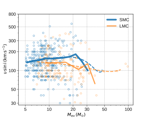
Figure 14: Projected rotational velocities of OB stars as functions of stellar mass (blue circles) on logarithmic scales. The LMC OB star sample (Ramachandran et al. 2018b) is also shown for comparison. Solid lines represent mean velocities averaged over logarithmic mass bins, while dashed lines give nonlinear fits to the data.

5.3 Impact of stellar rotation

The distribution of stellar rotation rates of our sample stars show a bimodal distribution (see Sect. 4.1). Approximately 30% of stars in the secondary peak are Be stars, which rotate close to their critical velocity. It is likely that some of the fast rotating stars, including members of the Be class, experienced binary interaction during their evolution (de Mink et al. 2013). According to single-star evolutionary tracks, their evolutionary masses range from 6 to 25 $M_{\odot}$ and they reside close to the TAMS (indicated by the hooks in the evolutionary tracks in Figure 13). These Be stars are also likely evolving toward a YSG/RSG phase.

Figure 14 shows $\varv\sin i$ for our sample of stars versus their evolutionary mass. First, we consider stars with masses above $30\,M_{\odot}$. The $\varv\sin i$ values for these stars decline sharply with mass and become relatively low. Such slow rotators are not expected to experience QCHE. Yet, we do see these stars close to the QCHE tracks in the HRD, suggesting that the mixing is not solely associated with rotation. Second, we consider stars with lower masses, $M_{\rm init}\sim 17-25\,M_{\odot}$. Among these stars are a group of fast rotating OB stars with $\varv\sin i$ in the range 300–550 km s^-1. Despite their fast rotation, these stars do not follow QCHE tracks, but are located on the cool side of the ZAMS. Therefore, we conclude that SMC stars with $M_{\rm init}\lesssim 30\,M_{\odot}$ follow standard evolution, independent of their current rotation rates.

The evolution of a star depends on its initial rotation rather than the current rotation. Unfortunately, it is hard to get a good handle on the initial rotation velocity of a star. It is different from the measured surface rotation because stellar mass loss (through line driven winds, mechanical mass loss by fast rotation, or induced by close binary evolution) can slow down the star throughout its evolution. We can state that our sample stars are still young and that their present-day mass-loss rates are very small (see Sect. 6). Hence, in case their present mass-loss rate would be representative for their whole previous lifetime, we would not expect a significant loss of angular momentum. We conclude that the evolutionary dichotomy observed in the HRD is independent of rotation.

Significantly, the upper limits on the rotational velocities of WR stars in the SMC are lower than that predicted for QCHE (Hainich et al. 2015). We may speculate that these WN stars had higher rotational velocities while on the ZAMS, but had slowed down since then. Our measurements of massive O stars do not support this (Fig. 14); a similar trend is also observed at LMC metallicity (Ramachandran et al. 2018b). Therefore, rapid rotation alone cannot be the crucial factor responsible for the observed dichotomy. Our results confirm the spectropolarimetric study of WR stars in Magellanic clouds, where no evidence for rotationally induced QCHE was found (Vink & Harries 2017).

5.4 Impact of a companion

Stellar evolution is also affected by the presence of a companion. So, the mass transfer in close binaries could also be another channel for the formation of WR stars. However, this channel cannot explain the apparently single massive WR stars in the SMC, which are all very massive and contain hydrogen, exactly as predicted by QCHE models. In case of WR stars in binary systems the situation is different.

While the spectra of our sample OB stars are satisfactorily fit by single-star models and do not clearly indicate binarity, it is likely that many of our targets are in fact binary systems (Sana et al. 2012). According to the Optical Gravitational Lensing Experiment (OGLE) survey (Pawlak et al. 2016), about 7% of our sample are eclipsing binaries, setting a firm lower limit on the binary fraction. A significant binary fraction may indeed affect our results. Our derived luminosities would be overestimated (e.g., by 0.3 dex for a binary with two identical stars) and this may result if the continuum of a companion dilutes the emission line spectrum. Lower luminosities would imply lower masses, and the uncertainty in $T_{\ast}$ is irrelevant in the context of the observed dichotomy. We conclude that our main results are not affected by uncertain binary statistics. However, close binary evolution can produce stars that occupy the same positions on the HRD as single stars, for example, via merging. In this case, single-star evolutionary models can mislead the interpretation. At present, the physics of merging is not well understood, but it is important to keep in mind that, in principle, merger products could contaminate our sample, for example, as extraluminous BSGs (Menon & Heger 2017; Farrell et al. 2019).

Summarizing, our empirical HRD of the SMC and comparisons with evolutionary tracks indicate two different paths of massive star evolution at low metallicity. Stars with initial mass below $30\,M_{\odot}$ evolve without full mixing toward a RSG phase, where they are likely to explode as SN II-P. In contrast, massive single stars ($M\gtrsim 30M_{\odot}$) expand only a little during their main sequence evolution, and then evolve toward WR stages remaining mixed, hot, and compact, in accordance with the predictions of the QCHE model. The lack of SNe with corresponding progenitors provides support to the idea that stars at the end of their QCHE may collapse to black holes directly (Heger et al. 2003; Marchant et al. 2016; Hainich et al. 2018). We suggest that the main factors for the evolutionary dichotomy are low metallicity and the initial mass of the star, rather than rotation.

6 Weak winds of massive stars at low metallicity

The spectroscopic analysis allows us to quantitatively measure stellar mass-loss rates. Observations in the UV are especially suitable for this. For nine stars with available UV spectra (see Sect. 2), we supplemented the optical spectra with the UV observations, and analyzed these spectra in a consistent manner using various diagnostic lines. Figure 15 shows the mass-loss rate ($\dot{M}$) versus luminosity of these nine OB stars (B2 to O3). A linear regression to this $\log\dot{M}-\log L$ relation, which accounts for the individual error bars, shows an order of magnitude systematic offset compared to the theoretical predictions (Vink et al. 2001) for SMC OB stars. The only exception is an Of supergiant (green diamond in Fig. 15). Excluding this star would result in an even higher offset compared to the predictions. Our results confirm previous spectroscopic studies of massive stars in the SMC (Bouret et al. 2003; Martins et al. 2004) and other low-metallicity dwarf galaxies like IC 1613 and WLM (Bouret et al. 2015; Lucy 2012). This is also in agreement with X-ray observations of NGC602 cluster (Oskinova et al. 2013), where they revealed that the emission is mainly coming from young low-mass stars, while the winds of the massive stars are not sufficient to power the detected extended X-ray emission.

In many OB-type dwarfs, the mass-loss rates derived empirically are much lower than predicted by the standard mass-loss recipes. At solar metallicity (or even LMC), this problem is limited to the late O- and early B-type dwarfs, and is often dubbed as the weak wind problem (Martins et al. 2005; Marcolino et al. 2009; Oskinova et al. 2011).

Among our subsample of OB stars with UV-based mass-loss rates, eight out of nine stars exhibit the weak wind phenomenon (cf. Fig. 15), with the exception of the supergiant SMCSGS-FS 310. The objects with weak wind comprise not only dwarfs, but also one star of luminosity class III (SMCSGS-FS 288). One of the stars (the most luminous one indicated in Fig. 15) has even the very early subtype O3 (SMCSGS-FS 231). In support of our finding, we mention that Bouret et al. (2013) obtained a low $\dot{M}$ even for the most luminous O-star in the SMC, MPG 355. Thus, it seems that at SMC metallicity the weak-wind phenomenon is ubiquitous, and concerns all OB subtypes and all luminosities except supergiants.

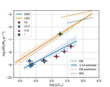
Figure 15: Mass-loss rate as a function of stellar luminosity for the analyzed SMC OB stars with available UV data. Luminosity classes are distinguished by different symbols as given in the legend. A power-law fit to the empiric relation is represented by the blue solid line. For comparison, we include the empirical relation for LMC OB stars (Ramachandran et al. 2018b) along with theoretical predictions (Vink et al. 2001) (dotted lines) at SMC and LMC metallicities. The empirical relations for WN stars in the SMC and LMC (Hainich et al. 2017) are also illustrated in the plot (dashed lines).

All hot star winds are clumpy (Hamann et al. 2008; Puls et al. 2008). Our model calculations account for such inhomogeneities in the microclumping approximation. We adopt depth dependent clumping with a density contrast $D=10$ (i.e. volume filling factor $f=0.1$). Details were given in Sect. 3.1. Clumping enhances emission lines which are fed by recombination cascades (Hamann & Koesterke 1998). Compensating for this effect, one derives a mass-loss rate that is smaller by the factor $\sqrt{D}$ than with a smooth-wind model. Such clumping dependence would apply if we would have derived $\dot{M}$ from, e.g., an H$\alpha$ emission line.

Fortunately, our empirical mass-loss rates shown in Fig. 15 and discussed above have been derived from resonance lines in the UV. These wind lines are mainly formed by line scattering. Since the corresponding opacities scale linearly with density, these lines do not react on microclumping at all. Hence, the mass-loss rates we obtained are independent of the adopted clumping parameters.

Theoretical considerations predict a power-law dependence of the mass-loss rate on metallicity, $\dot{M}\propto Z^{\alpha}$, with $\alpha$=0.69 for O-type stars (Vink et al. 2001), whereas empirical studies found $\alpha$=0.83 (Mokiem et al. 2007). However, our analysis suggests a much steeper relation with $\alpha\sim 2$. The WN winds show a metallicity dependence of $\dot{M}\propto Z^{1.2}$ (Hainich et al. 2017). Since WR winds are much stronger than the winds of O stars, it is important to consider by how much the mass loss increases while a star evolves from the O to the WR stage. Figure 15 shows empirical and theoretical mass-loss rates for O and WR stars in the LMC and SMC. It is striking that the difference between mass-loss rates of O and WR stars is significantly larger at the lower SMC metallicity compared to the LMC.

Very weak winds of OB stars should have only low impact on their fates. However, it may change our current understanding on stellar evolution, because theoretical evolutionary tracks, as a rule, are calculated using the standard mass-loss recipes, and hence are based on strongly overestimated mass-loss rates. After the first detection of gravitational waves, it has been argued that black hole pairs as massive as $60\,M_{\odot}$ can only form if the mass loss is relatively low (Abbott et al. 2016). For instance, according to SMC metallicity tracks by Eldridge et al. (2008), a star with initially $60\,M_{\odot}$ ends with only $22\,M_{\odot}$ short before core collapse. This prediction depends on the adopted mass-loss rate prescriptions for the different evolutionary phases. Additionally, a star might loose a significant amount of mass by eruptions in the LBV stage (Smith & Owocki 2006), which is not taken into account by standard tracks. However, if a star evolves quasi chemically homogeneously, the phase of LBV instability can be avoided. The weak winds in the OB phase reported here are not sufficient to remove the hydrogen envelope, and therefore not lead to a WR phase. This is in agreement with the suggested dichotomy in evolution, where apparently single WR stars are formed by strong internal mixing. Very weak OB winds and QCHE above a certain mass limit suggest that massive black holes can form even at SMC-like metallicity.

7 Mode of star formation in the SMC Wing

Spectroscopy of massive stars allows us to investigate the star formation modes in the SMC Wing and the SMC-SGS 1. Using the evolutionary tracks and isochrones (Brott et al. 2011), we estimated the individual ages of all OB stars (see Fig. 16, Table B). The uncertainties in the age are mostly in the range of 20-40%, which comes from the uncertainties in temperature, luminosity, and $\varv\sin i$. Five stars in this complex are found to be very young, and are less than 2 Myr in age, including the O3-type star (Sk 183) in NGC 602. From ages and masses of the individual OB stars, and by extrapolation to lower masses ($0.5\,M_{\odot}$) using the Salpeter initial mass function (IMF), we estimate the present day star formation rate (SFR) of the complex to be $\approx 10^{-3}\,M_{\odot}\,\mathrm{yr}^{-1}$. With the area of the two observed fields in SMC-SGS 1 ($\sim$0.2 kpc²) the SFR surface density becomes $\approx 4\times 10^{-3}\,M_{\odot}\,\mathrm{yr}^{-1}\,\mathrm{kpc}^{-2}$.

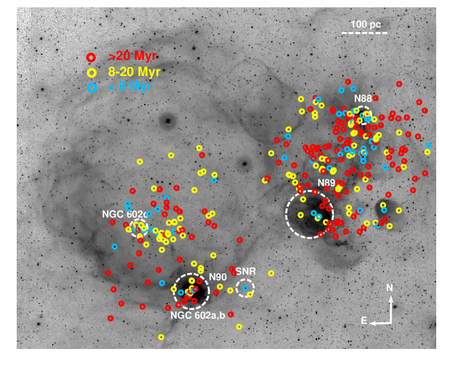
Figure 16: Distribution of the OB stars in the SGS, color coded with their age

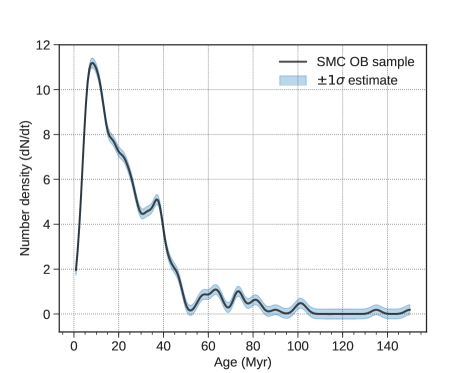
Figure 17: Distribution of stellar ages of OB stars in our sample

A comparison of the empirical HRD with the evolutionary isochrones gives an age spread from 0 to 100 Myr for the OB stars in the complex. The age histogram (Fig. 17) indicates persistent star formation in this large-scale low density region over a long time. The distribution shows active star formation ongoing since 30–40 Myr, with a peak at about 6–7 Myr ago. Of course, the present age distribution is biased by the expired lifetimes of the more massive stars. It is tempting to suggest that the feedback from massive stars that formed 30–40 Myr ago, but already disappeared, have created this SGS, which expands and triggers the formation of present massive stars near its rim. However, as can be seen from Fig. 16, there is no obvious age gradient across the SMC-SGS 1 (see also Fulmer et al. 2019 submitted). We found many young massive stars close to the central parts of the complex, especially in the NGC 602c cluster, and also in the western regions near N 88. On the other hand, there is a high concentration of the relatively old B-star population in the western nebular regions. Such spatial distribution in the complex nullifies SGS induced star formation at the rim. Instead, it supports a stochastic mode of star formation. Altogether, we invalidate the central source/cluster scenario for the formation of the SGS. Moreover, we found that the H$\alpha$ emission in the complex does not fully trace the distribution of young massive stars. Only faint, filamentary H$\alpha$ emission is observed in the central part of SGS, which hosts a relatively high number of young massive stars.

We ask ourselves whether the apparent dichotomy in the empirical HRDs (Figs. 13 and 18) in fact reflects a specific star formation history instead of a bifurcation in stellar evolution. We believe that this is unlikely because the stars in the empirical HRD are located in different parts of the SMC; while our OB star sample is in the Wing of the SMC, other stars are distributed throughout the SMC and include runaway and cluster members. Therefore, there is no reason to suspect that all stars with masses above $\sim 30\,M_{\odot}$ are produced in the same coherent star burst episodes.

8 Feedback from massive stars and the energy budget of the supergiant shell

The total ionizing photon flux produced by all the OB stars in our sample is $\Sigma Q\approx 8\times 10^{49}\,\rm{s^{-1}}$, and 30% are contributed by the O3 star located in NGC 602 alone. The SGS also encompasses AB 8, the WO-type binary in the NGC 602c cluster. By releasing a hydrogen ionizing photon flux of $Q\approx 1.5\times 10^{50}\,\rm{s^{-1}}$ and He ii ionizing photon flux of $\approx 5\times 10^{47}\,\rm{s^{-1}}$, the WO+O4 system dominates the radiative feedback in SMC-SGS 1 (Shenar et al. 2016). However, the H ii region associated with NGC 602c and its WO binary consists only of small, relatively faint emission regions scattered around the cluster. The integrated H$\alpha$ luminosity of the SGS (Kennicutt et al. 1995) corresponds to an ionizing photon flux of $Q$ = $10^{50}$ s^-1. This is only half of the total Lyman continuum flux emitted by the stars we analyzed.

The winds of SMC OB stars are quite weak (Sect. 6). Therefore it is not surprising that the mechanical feedback by OB stars in this region is significantly lower than in star-forming regions in the LMC (Ramachandran et al. 2018b) and the Galaxy. The total mechanical luminosity generated by all OB stars in our sample is estimated to be $\Sigma L_{\rm mec}=\Sigma\,0.5\,\dot{M}\,\varv_{\infty}^{2}\sim\,3\times 10^{35}\rm{erg\,s^{-1}}$. The accumulated mechanical energy from all sample OB stellar winds throughout their life is $\Sigma E_{\rm mec}=\Sigma\,0.5\,\dot{M}\,\varv_{\infty}^{2}t\,\approx 6\times 10^{49}\,\rm{erg}$. We estimate the radial momentum contribution to be $\Sigma p=\dot{M}\,\varv_{\infty}t\,\approx 5\times 10^{41}\,\rm{g\,cm\,s^{-1}}$. We emphasize that these feedback estimates only consider current OB stars in the complex and do not account for those massive stars that already disappeared. In addition, our sample does not include massive stars in the northern regions of the SGS.

The WO+O system, AB 8, alone supplies a current mechanical luminosity of $\approx 7\times 10^{37}\,\rm{erg\,s^{-1}}$. This is more than two orders of magnitude higher than the mechanical luminosity produced by all 320 OB stars in the sample together. In order to estimate the mechanical energy released by the WO star during its lifetime, we need information about its progenitor. We estimated this with the help of binary evolutionary tracks (Eldridge & Stanway 2009), by giving the current parameters of the primary and secondary as input. The mechanical energy contribution is $\approx 1.6\times 10^{51}\rm{erg}$ in the pre-WR phase and $\approx 4\times 10^{50}\rm{erg}$ in the WR phase. Interestingly, the accumulated energy and momentum from this WO binary are also two orders of magnitude higher than those generated from all OB stars together (see Table 1). Hence, a single WR star (contribution of the secondary is negligible) is responsible for the vast majority of feedback in the complex, exceeding by far from the contribution from the whole OB population (see Table 1). Existing X-ray observations do not detect diffuse emission from a hot wind blown bubble around AB 8 or in the SMC-SGS 1 (Oskinova et al. 2013). This is possibly due to the low density in the SGS, or to leakage of hot gas.

To estimate the full energy budget in the SGS, knowledge of SN rate in the complex is required. Two confirmed high mass X-ray binaries (HMXBs) in this complex serve as an evidence for past SNe. Interestingly, these HMXBs, SXP 1062 and RX J0123.4-7321, are located outside of the SGS. Following our empirical HRD (Sect. 5), stars with masses in the range of 8 to $30\,M_{\odot}$ become SNe II-P. There are about 190 such stars in our sample as well as additional B stars without spectra in the photometric study (Fulmer et al. 2019 submitted) which will become SNe II-P in the next 40 Myr. Thus the current rate is $\gtrsim 5$ SNe per Myr, assuming a constant SFR. If we only consider stars that are located inside the SGS, the rate becomes $\gtrsim 2.5$ per Myr. This is a lower limit since our spectroscopic survey did not cover the full extent of the SGS.

It is difficult to accurately estimate the age of SMC-SGS 1. We do not detect SN remnants or HMXBs within the shell, and there is a high likelihood of off-center SNe along with the possibility of molecular clouds inside the shell that add extra cooling. It seems that an age of 20-40 Myr is likely (Fulmer et al. 2019 submitted), which is in line with the dynamic age of the shell and the age of the stellar population (Fig. 17). We adopt an age of 30 Myr for the feedback estimates, which is also the time-scale of active star formation in the complex. According to our estimated rate, at least 75 SNe must have contributed to the feedback in the SGS. A typical SNe II-P releases $10^{51}$ erg. The accumulated mechanical energy by SNe is then $E_{\rm{mec}}\approx 7.5\times 10^{52}\,\rm{erg}$, which is huge compared to stellar wind contribution. However, the energy released by the SNe reduces over time owing to radiative cooling. In low density and low-metallicity environments, the radiative losses are small (Geen et al. 2015). Therefore, in 30 Myr , the SN energy may decline only up to $E_{\rm{SN}}\approx 10^{50}\,\rm{erg}$. Considering this effect, the total energy feedback from SNe to the SMC-SGS 1 becomes $\approx 10^{52}\,\rm{erg}$. Supernovae also injects a huge amount of momentum into the ISM and drive turbulence, which cannot be radiated away (Geen et al. 2015). Following Kimm & Cen (2014) and Kimm et al. (2015), the total momentum released by SNe is $p\approx 5\times 10^{45}\,\rm{g\,cm\,s^{-1}}$. This is again significantly higher than the momentum provided by massive star winds.

Table 1: Ionizing flux, mechanical luminosity, momentum, and accumulated mechanical energy contributions by the OB stars, WO binary, and previous SNe, compared to the values observed in the SGSl.

	$Q$	$L_{\rm mec}$	$p$	$E_{\rm mec}$
	[s-1]	[erg s-1]	$[\rm{g\,cm\,s^{-1}}$]	[erg]
OB	$8\times 10^{49}$	$3\times 10^{35}$	$5\times 10^{41}$	$6\times 10^{49}$
WO	$1.5\times 10^{50}$	$7\times 10^{37}$	$1.4\times 10^{43}$	$2\times 10^{51}$
SN			$5\times 10^{45}$	$10^{52}$
Total	$2\times 10^{50}$	$7\times 10^{37}$	$5\times 10^{45}$	$1.2\times 10^{52}$
Observation	$\sim 10^{50}$	$<5\times 10^{32}$	$6\times 10^{45}$	$6\times 10^{51}$

From neutral hydrogen observations, the surface density of the H i shell is $\sim 3\,M_{\odot}$ pc^-2 (Stanimirovic et al. 1999; Fulmer et al. 2019 submitted). With a radius of about 300 pc, the total mass of H i gas in the SGS is $M_{\rm SGS}\sim 3\times 10^{6}\,M_{\odot}$. At an expansion velocity of 10 km s^-1, the total momentum and kinetic energy in the SGS is about $p_{\rm SGS}\approx 6\times 10^{45}\,\rm{g\,cm\,s^{-1}}$ and $E_{\rm SGS}\approx 6\times 10^{51}\rm{erg}$, i.e, comparable to the contributions from SNe explosions in the past 30 Myr. The kinetic energy of the expanding SGS is a factor of two smaller compared to the estimated mechanical energy input. This might be because of radiative cooling or leakage of hot gas. These estimates show that the SN feedback plays a crucial role in the formation of the SMC-SGS 1.

Table  1 summarizes the estimated energy feedback from OB stars, WR stars, and SNe and includes a comparison with values derived from observations in the SGS. In our study of massive stars in the LMC superbubble N 206 (Ramachandran et al. 2018a, b) we found that the contribution of young OB stars is very high in terms of both ionizing photon flux and mechanical luminosity. The contributions from massive stars and SNe were almost equal, while this SMC study reveals a different feedback situation. In SMC-SGS 1, the WO star dominates all other OB stars in terms of ionization and mechanical feedback. The energy and momentum contribution from SNe over the last 30 Myr (age of the SGS) is significantly higher than the stellar wind feedback in the complex and this contribution is similar to the observed energy and momentum stored in the SGS. We conclude that at low-metallicity dwarf galaxies, SN explosions seem to be the dominant source for most of the mechanical feedback. The low levels of feedback in metal-poor stellar populations may promote the growth and survival of molecular clouds, thereby allowing star formation episodes to persist over long timescales. Such extended star formation can result in a continuous supply of ionizing photons, which can leak out into the circumgalactic medium via SN created holes or channels.

9 Summary

We present the results of a spectroscopic survey of massive stars in the SMC Wing. The spectra of 320 OB stars were analyzed using modern stellar atmosphere models to derive their fundamental stellar parameters as well as their contributions to feedback through ionizing radiation and stellar winds. We derive calibrations for the temperature and ionizing flux of OB stars as a functions of their spectral subtype. Complementing the results of our study by previous analyses of evolved massive stars in the WR and RSG evolutionary stages, we obtain a well-populated empiric HRD of massive stars in the SMC.

Comparison with evolutionary tracks reveals an apparent dichotomy in massive star evolution: stars initially less massive than $30\,M_{\odot}$ evolve to red supergiants. These stars are likely SNe II-P progenitors. In contrast, stars (single) initially more massive than $30\,M_{\odot}$ likely follow a QCHE. These stars might collapse and form black holes directly, without a SN explosion.

We find no evidence that the most-massive SMC stars evolving quasi-chemically homogeneously are fast rotators. Also, we do not find evidence that the fast rotating stars among the less massive objects evolve quasi-chemically homogeneously. Hence, there is no empirical support for the idea that QCHE is governed mainly by rotation. The bifurcation in evolutionary paths rather seems to be unrelated to rotation. We suggest that the main factors for the evolutionary dichotomy are low metallicity and the initial mass of the star.

The mass-loss rates of OB stars empirically estimated from the spectral analysis are significantly lower than theoretically predicted. This result calls for a revision of stellar evolutionary calculations that routinely rely on overestimated mass-loss rates at low metallicities.

The ages and spatial distribution of massive stars in the SMC Wing shows that star formation is proceeding in this quiescent low density region since more than 100 Myr, and suggests that massive star formation is stochastic there and not spatially progressing. The weakness of OB-star winds at low metallicity make the SN explosions the dominant sources of mechanical energy and momentum input into the ISM. However, we find that the large population of OB stars produced during the star formation peak in the past $\sim$50 Myr is fully capable of producing the SMC-SGS 1 supershell. Star-forming complexes with extended histories will leave their mark on the surrounding ISM even in low-metallicity systems.

Appendix A Additional figures

Appendix B Additional tables

Table 2: Stellar parameters of all OB stars in the SMC-SGS 1

SMCSGS-FS	Spectral type	$T_{\ast}$	$\log\,L$	$\log\,g_{\ast}$	$\log\,\dot{M}$	$E_{\rm B-V}$	$M_{\mathrm{V}}$	$R_{\ast}$	$\varv_{\infty}$	$\varv\,\sin\,i$	$\varv_{\rm rad}$	$M_{\ast}$	$\log\,Q_{0}$	$\log\,L_{\mathrm{mec}}$
#		[kK]	[$L_{\odot}$]	[cm s-2]	[$M_{\odot}\,\mathrm{yr}^{-1}$]	[mag]	[mag]	[$R_{\odot}$]	[km s-1]	[km s-1]	[km s-1]	[$M_{\odot}$]	[s-1]	[$L_{\odot}$]
1	B0.7 V	27	3.83	4.4	$-9.5$	0.03	$-1.8$	3.8	2300	120	170	13	46.1	$-1.9$
2	B0.2 V	29	4.21	4.4	$-9.1$	0.02	$-3.0$	5.1	2600	80	160	23	46.7	$-1.2$
3	B2.5 V	19	3.52	4.0	$-9.8$	0.03	$-2.2$	5.3	900	130	150	10	44.5	$-2.4$
4	B2 III	19	4.27	3.4	$-9.0$	0.03	$-3.8$	12.6	600	130	160	15	45.4	$-1.1$
5	B2 V	20	3.56	4.2	$-9.7$	0.05	$-1.9$	5.0	1100	100	170	15	44.6	$-2.4$
6	B1.5 IV	23	3.87	4.0	$-9.4$	0.03	$-3.0$	5.4	1700	70	170	11	45.6	$-1.8$
7	B2 V	22	3.76	4.2	$-9.5$	0.05	$-2.2$	5.2	2200	70	170	16	45.2	$-2.0$
8	B2 V	20	3.66	4.2	$-9.6$	0.05	$-2.0$	5.6	1100	130	120	18	44.7	$-2.2$
9	B2 (IV)e	22	4.01	3.8	$-9.3$	0.09	$-2.8$	7.0	1500	250	170	11	45.6	$-1.6$
10	B7 V	14	3.12	3.8	$-10.2$	0.05	$-2.0$	6.2	800	80	170	9	43.7	$-3.1$
11	B2 V	20	3.66	4.2	$-9.6$	0.05	$-2.0$	5.6	1100	100	170	18	44.7	$-2.2$
12	B8 V	14	3.22	3.8	$-10.1$	0.05	$-2.1$	6.9	800	100	170	11	43.8	$-3.0$
13	B1.5 IV	22	4.08	3.6	$-9.2$	0.03	$-3.0$	7.6	1200	140	155	8	45.7	$-1.4$
14	B2.5 V	19	3.52	4.0	$-9.8$	0.05	$-2.2$	5.3	900	200	170	10	44.5	$-2.4$
15	B2.5 IV	20	3.63	3.6	$-9.7$	0.10	$-2.2$	5.5	500	140	160	4	44.9	$-2.2$
16	B1.5 V	22	4.11	3.8	$-9.2$	0.05	$-3.1$	7.8	1600	150	200	14	45.7	$-1.4$
17	B5 V	16	3.52	4.0	$-9.8$	0.05	$-2.3$	7.5	1000	130	140	21	44.2	$-2.4$
18	B1.5 (IV)e	24	4.44	3.8	$-8.9$	0.09	$-3.5$	9.6	1800	320	170	21	46.4	$-0.8$
19	B5 V	16	3.32	4.0	$-10.0$	0.02	$-2.4$	6.0	900	150	120	13	44.0	$-2.8$
20	B5 V	16	3.12	4.0	$-10.2$	0.05	$-1.9$	4.7	800	140	160	8	43.8	$-3.1$
21	B5 V	16	3.32	4.0	$-10.0$	0.03	$-1.8$	6.0	900	200	190	13	44.0	$-2.8$
22	B0.5 V	27	4.54	4.0	$-8.8$	0.04	$-3.8$	8.5	2100	80	170	27	46.9	$-0.6$
23	B9 III	11	3.02	3.5	$-10.3$	0.03	$-2.2$	8.9	600	110	180	9	43.0	$-3.3$
24	B7 V	14	3.42	3.8	$-9.9$	0.05	$-1.9$	8.7	900	100	160	18	44.0	$-2.6$
25	B3 V	18	3.32	3.8	$-10.0$	0.05	$-2.0$	4.7	600	180	170	5	44.3	$-2.8$
26	B5 V	17	3.45	3.8	$-9.9$	0.04	$-1.9$	6.1	700	160	190	9	44.4	$-2.6$
27	B2.5 V	19	3.52	4.2	$-9.8$	0.05	$-1.9$	5.3	1100	140	170	16	44.4	$-2.4$
28	B5 V	17	3.65	3.8	$-9.7$	0.05	$-2.7$	7.7	800	220	160	14	44.6	$-2.2$
29	B0.7 V	26	4.02	4.4	$-9.3$	0.03	$-2.6$	5.1	2700	230	170	23	46.2	$-1.5$
30	B1 V	26	3.7	4.4	$-9.6$	0.02	$-2.0$	3.5	2200	70	170	11	45.9	$-2.1$
31	O9 V	32	4.93	4.0	$-8.4$	0.02	$-4.3$	9.5	2000	340	160	33	48.1	$0.1$
32	B0.7 (III)e	25	4.72	3.6	$-8.6$	0.22	$-4.2$	12.2	1500	280	170	22	46.9	$-0.3$
33	B3 V	17	3.65	3.8	$-9.7$	0.05	$-2.1$	7.7	800	50	160	14	44.6	$-2.2$
34	B3 (V)e	18	3.52	3.8	$-9.8$	0.08	$-2.0$	5.9	700	200	170	8	44.5	$-2.4$
35	B1.5 V	22	3.76	4.2	$-9.5$	0.05	$-2.6$	5.2	2200	180	170	16	45.2	$-2.0$
36	B0.5 (III)e	26	5.23	3.2	$-8.1$	0.19	$-5.1$	20.4	1000	300	160	24	47.8	$0.6$
37	B0.7 V	26	4.14	4.2	$-9.2$	0.05	$-3.1$	5.8	2200	330	170	20	46.3	$-1.3$
38	B0.2 V	28	4.37	4.2	$-8.9$	0.02	$-3.0$	6.5	2300	80	150	25	46.8	$-0.9$
39	B0.5 V	27	4.29	4.2	$-9.0$	0.02	$-3.0$	6.4	2300	230	170	24	46.6	$-1.1$
40	B0.7 V	25	4.29	4.0	$-9.0$	0.05	$-3.6$	7.5	2000	130	170	20	46.4	$-1.1$
41	B2.5 V	19	3.22	4.2	$-10.1$	0.03	$-1.5$	3.8	900	160	170	8	44.1	$-3.0$
42	B2 IV	20	4.03	3.8	$-9.3$	0.05	$-3.1$	8.6	900	80	170	17	45.1	$-1.5$
43	B2 (V)e	20	4.01	3.8	$-9.3$	0.11	$-3.3$	8.4	900	180	170	16	45.7	$-1.6$
44	B0 V	30	4.51	4.2	$-8.8$	0.03	$-3.6$	6.7	2300	130	160	26	47.2	$-0.7$
45	B2 Ib	20	4.42	2.8	$-8.9$	0.45	$-3.5$	13.5	300	50	170	4	45.7	$-0.8$
46	B0 V	30	4.3	4.4	$-9.0$	0.02	$-3.2$	5.2	2600	250	170	25	46.9	$-1.0$
47	B2 V	22	3.86	4.2	$-9.4$	0.03	$-2.7$	5.9	2300	70	140	20	45.3	$-1.8$
48	B2 V	22	3.96	4.2	$-9.3$	0.05	$-3.0$	6.6	2400	130	160	25	45.4	$-1.7$
49	B3 (IV)e	17	3.75	3.4	$-9.6$	0.23	$-2.6$	8.7	500	150	170	7	44.7	$-2.0$
50	B9 Ib	10	3.72	2.8	$-9.6$	0.03	$-3.6$	24.2	500	80	200	13	43.3	$-2.1$
51	B1.5 (V)e	22	4.21	3.8	$-9.1$	0.08	$-3.0$	8.8	1700	250	170	18	45.8	$-1.2$
52	B0.5 V	28	4.03	4.4	$-9.3$	0.05	$-2.6$	4.4	2500	150	170	18	46.4	$-1.5$
53	B2 V	19	3.52	4.0	$-9.8$	0.02	$-2.0$	5.3	900	80	170	10	44.5	$-2.4$
54	B1.5 V	23	3.66	4.4	$-9.6$	0.05	$-2.0$	4.3	2500	220	160	17	45.1	$-2.2$
55	B1.5 IV	22	4.18	3.6	$-9.1$	0.02	$-3.6$	8.5	1300	270	100	10	45.8	$-1.3$
56	B0.5 V	28	3.81	4.4	$-9.5$	0.09	$-2.0$	3.4	2200	100	150	11	46.2	$-1.9$
57	B5 V	16	3.22	4.0	$-10.1$	0.03	$-2.1$	5.3	900	120	160	10	44.0	$-3.0$
58	B2.5 V	19	3.32	4.2	$-10.0$	0.05	$-2.2$	4.2	1000	140	160	10	44.2	$-2.8$
59	B0 V	29	4.42	4.2	$-8.9$	0.05	$-3.3$	6.4	2300	200	170	24	47.0	$-0.8$
60	B0.2 V	28	3.93	4.4	$-9.4$	0.05	$-2.6$	3.9	2300	120	170	14	46.3	$-1.7$
61	B1.5 V	23	4.07	4.0	$-9.2$	0.02	$-4.1$	6.8	1900	80	160	17	45.8	$-1.5$
62	B0 V	29	4.46	4.2	$-8.9$	0.05	$-3.7$	6.7	2300	140	170	26	47.0	$-0.8$
63	B0.5 V	27	4.03	4.4	$-9.3$	0.05	$-2.6$	4.7	2600	100	160	21	46.3	$-1.5$
64	O9 V	33	5.05	4.0	$-8.3$	0.05	$-4.6$	10.3	2000	50	120	39	48.3	$0.3$
65	B0.2 V	29	4.11	4.4	$-9.2$	0.03	$-2.7$	4.5	2500	120	170	19	46.6	$-1.4$
66	B2 V	19	3.92	4.2	$-9.4$	0.09	$-2.5$	8.4	1400	250	170	41	44.8	$-1.7$
67	B0 V	31	4.6	4.2	$-8.7$	0.05	$-3.9$	6.9	2300	70	150	28	47.5	$-0.5$
68	B2 V	20	3.56	4.2	$-9.7$	0.05	$-2.0$	5.0	1100	130	160	15	44.6	$-2.4$
69	B0.5 (II)e	26	5.05	3.2	$-8.3$	0.05	$-5.0$	16.6	900	100	160	16	47.6	$0.3$
70	B0 V	30	4.56	4.2	$-8.8$	0.05	$-3.4$	7.1	2300	170	160	29	47.3	$-0.6$
71	B1.5 IV	22	3.61	3.8	$-9.7$	0.05	$-2.0$	4.4	1200	250	160	4	45.2	$-2.3$
72	B2 (II)e	18	4.2	3.0	$-9.1$	0.05	$-3.9$	13.0	400	150	170	6	45.2	$-1.2$
73	B0 (IV)e	30	5.02	3.8	$-8.3$	0.08	$-4.6$	12.0	1700	270	160	33	48.0	$0.2$
74	B2 V	19	3.52	4.2	$-9.8$	0.02	$-2.2$	5.3	1100	160	170	16	44.4	$-2.4$
75	B1.5 V	22	3.86	4.2	$-9.4$	0.05	$-2.2$	5.9	2300	250	170	20	45.3	$-1.8$
76	B0.7 V	26	3.96	4.2	$-9.3$	0.03	$-2.7$	4.7	2000	160	150	13	46.1	$-1.7$
77	B1.5 IV	22	4.27	3.8	$-9.0$	0.02	$-3.8$	9.4	1800	160	150	20	45.9	$-1.1$
78	B2 V	20	3.56	4.2	$-9.7$	0.03	$-2.2$	5.0	1100	140	160	15	44.6	$-2.4$
79	B2.5 V	19	3.52	4.2	$-9.8$	0.05	$-2.2$	5.3	1100	120	160	16	44.4	$-2.4$
80	B2.5 V	19	3.52	4.0	$-9.8$	0.07	$-2.3$	5.3	900	160	160	10	44.5	$-2.4$
81	B1.5 V	23	3.96	4.4	$-9.3$	0.05	$-1.9$	6.0	3000	180	190	33	45.4	$-1.7$
82	B2 IV	20	3.83	3.6	$-9.5$	0.08	$-2.7$	6.9	600	120	160	7	45.1	$-1.9$
83	B1.5 V	23	3.76	4.4	$-9.5$	0.05	$-2.0$	4.8	2600	170	160	21	45.2	$-2.0$
84	B1.5 V	23	3.76	4.4	$-9.5$	0.05	$-2.2$	4.8	2600	250	170	21	45.2	$-2.0$
85	B0.7 V	26	4.19	4.2	$-9.1$	0.03	$-3.3$	6.2	2300	70	170	22	46.3	$-1.2$
86	B9 III	10	3.35	3.4	$-10.0$	0.03	$-2.9$	15.8	800	80	170	23	43.0	$-2.7$
87	B2 V	22	3.66	4.2	$-9.6$	0.03	$-2.4$	4.7	2000	120	180	13	45.1	$-2.2$
88	B0.5 V	26	3.72	4.4	$-9.6$	0.05	$-2.2$	3.6	2200	220	170	12	45.9	$-2.1$
89	O9.5 V	31	4.84	4.0	$-8.5$	0.02	$-5.1$	9.1	2000	120	160	31	47.8	$-0.1$
90	O9.7 V	31	4.9	4.0	$-8.4$	0.02	$-4.6$	9.8	2100	70	200	35	47.9	$0.0$
91	B0.7 (IV)e	25	4.35	3.8	$-9.0$	0.09	$-3.2$	8.0	1600	150	170	15	46.5	$-1.0$
92	B0.5 V	28	3.83	4.4	$-9.5$	0.05	$-2.4$	3.5	2200	90	160	11	46.2	$-1.9$
93	B2.5 V	19	3.42	4.2	$-9.9$	0.08	$-2.0$	4.7	1000	140	130	13	44.3	$-2.6$
94	B1.5 V	23	4.06	4.4	$-9.3$	0.05	$-3.1$	6.8	3100	80	160	42	45.5	$-1.5$
95	B1.5 V	23	3.76	4.4	$-9.5$	0.05	$-2.2$	4.8	2600	220	160	21	45.2	$-2.0$
96	B1.5 V	22	4.3	4.0	$-8.7$∗	0.08	$-3.7$	9.8	900∗	250	170	35	46.5	$-1.0$∗
97	B1.5 V	23	3.56	4.4	$-9.7$	0.05	$-1.6$	3.8	2300	170	170	13	45.0	$-2.4$
98	B0.5 V	26	4.08	4.2	$-9.2$	0.02	$-2.9$	5.4	2100	130	150	17	46.2	$-1.4$
99	B1 IV	24	4.69	3.6	$-8.6$	0.05	$-4.8$	12.8	1600	120	170	24	46.7	$-0.4$
100	B2.5 V	19	3.42	4.2	$-9.9$	0.02	$-2.2$	4.7	1000	180	160	13	44.3	$-2.6$
101	B2.5 V	20	3.56	4.2	$-9.7$	0.05	$-2.3$	5.0	1100	200	170	15	44.6	$-2.4$
102	B3 V	17	3.35	3.8	$-10.0$	0.02	$-1.8$	5.5	700	200	150	7	44.3	$-2.7$
103	B2.5 V	19	3.42	4.2	$-9.9$	0.05	$-2.0$	4.7	1000	150	140	13	44.3	$-2.6$
104	B5 V	16	3.02	4.0	$-10.3$	0.05	$-1.8$	4.2	800	250	160	7	43.8	$-3.3$
105	B2.5 V	20	3.76	4.2	$-9.5$	0.02	$-2.4$	6.3	1200	130	160	23	44.8	$-2.0$
106	B1.5 V	23	3.86	4.4	$-9.4$	0.02	$-2.1$	5.4	2800	180	160	27	45.3	$-1.8$
107	B0 V	31	4.62	4.2	$-8.7$	0.05	$-3.6$	7.1	2300	60	160	29	47.5	$-0.5$
108	B2.5 V	20	3.46	4.2	$-9.8$	0.04	$-2.0$	4.5	1000	140	170	12	44.5	$-2.5$
109	B2.5 V	19	3.62	4.2	$-9.7$	0.05	$-1.7$	6.0	1200	120	110	21	44.5	$-2.3$
110	B2.5 (III)e	18	3.9	3.2	$-9.4$	0.07	$-3.4$	9.2	400	220	160	5	45.0	$-1.8$
111	O8.5 V	35	4.73	4.4	$-8.6$	0.05	$-3.7$	6.3	2700	220	240	37	48.1	$-0.3$
112	B3 V	19	3.62	4.2	$-9.7$	0.05	$-2.1$	6.0	1200	100	160	21	44.5	$-2.3$
113	B7 V	13	2.72	3.8	$-10.6$	0.03	$-1.1$	4.5	600	100	110	5	43.2	$-3.8$
114	B2.5 V	19	3.52	4.0	$-9.8$	0.03	$-2.2$	5.3	900	200	170	10	44.5	$-2.4$
115	B1.5 V	22	3.46	4.2	$-9.8$	0.05	$-2.0$	3.7	1800	120	160	8	44.9	$-2.5$
116	B2.5 V	19	3.52	4.2	$-9.8$	0.03	$-2.0$	5.3	1100	80	160	16	44.4	$-2.4$
117	B5 (IV)e	16	3.82	3.4	$-9.5$	0.08	$-2.8$	10.6	600	180	170	10	44.8	$-1.9$
118	B2.5 V	19	3.67	4.0	$-9.6$	0.05	$-2.5$	6.3	1000	170	150	15	44.9	$-2.2$
119	B0 V	32	4.63	4.0	$-8.7$	0.05	$-3.3$	6.7	1700	250	160	17	47.8	$-0.5$
120	B0.2 V	29	4.44	4.2	$-8.9$	0.05	$-2.8$	6.6	2300	30	170	25	47.0	$-0.8$
121	O9.7 V	32	4.71	4.2	$-8.6$	0.05	$-3.9$	7.4	2300	50	170	32	47.8	$-0.3$
122	B2 V	20	3.46	4.2	$-9.8$	0.05	$-1.9$	4.5	1000	80	160	12	44.5	$-2.5$
123	B2 IV	20	3.93	3.6	$-9.4$	0.05	$-3.0$	7.7	600	100	170	9	45.2	$-1.7$
124	B2.5 (V)e	19	4.07	3.8	$-9.2$	0.08	$-2.9$	10.0	900	200	180	23	45.1	$-1.5$
125	B0.5 V	27	4.24	4.2	$-9.1$	0.05	$-2.7$	6.0	2300	220	160	21	46.5	$-1.2$
126	B5 V	16	3.42	3.8	$-9.9$	0.05	$-1.7$	6.7	800	100	160	10	44.3	$-2.6$
127	B2.5 V	20	3.83	3.8	$-9.5$	0.05	$-2.8$	6.9	800	280	160	11	44.9	$-1.9$
128	O9 V	34	4.72	4.2	$-8.6$	0.05	$-3.2$	6.6	2100	410	170	25	48.0	$-0.3$
129	B3 V	18	3.62	3.8	$-9.7$	0.05	$-2.6$	6.7	800	70	180	10	44.6	$-2.3$
130	B2.5 V	19	3.52	4.2	$-9.8$	0.02	$-2.1$	5.3	1100	160	160	16	44.4	$-2.4$
131	B1.5 V	22	3.46	4.2	$-9.8$	0.05	$-1.5$	3.7	1800	100	170	8	44.9	$-2.5$
132	B2 V	22	3.86	4.2	$-9.4$	0.05	$-2.4$	5.9	2300	150	170	20	45.3	$-1.8$
133	B2 V	22	3.86	4.2	$-9.4$	0.05	$-1.9$	5.9	2300	120	160	20	45.3	$-1.8$
134	B2.5 V	20	3.56	4.2	$-9.7$	0.05	$-1.8$	5.0	1100	200	160	15	44.6	$-2.4$
135	B2 IV	20	3.93	3.8	$-9.4$	0.05	$-3.1$	7.7	800	170	160	14	45.0	$-1.7$
136	B1 (IV)e	23	4.31	3.8	$-9.0$	0.05	$-3.2$	9.0	1700	120	170	19	46.2	$-1.0$
137	B1.5 IV	21	4.26	3.6	$-9.1$	0.05	$-3.6$	10.2	1500	180	170	15	45.7	$-1.1$
138	B1.5 V	22	3.76	4.2	$-9.5$	0.05	$-2.1$	5.2	2200	270	140	16	45.2	$-2.0$
139	B2.5 (V)e	20	3.73	3.8	$-9.6$	0.08	$-2.3$	6.1	700	150	170	9	44.8	$-2.1$
140	B2 V	20	3.64	4.2	$-9.7$	0.05	$-2.0$	5.5	1100	80	160	18	44.7	$-2.2$
141	B1.5 V	22	3.96	4.2	$-9.3$	0.05	$-3.0$	6.6	2400	200	170	25	45.4	$-1.7$
142	B2 V	21	3.86	4.0	$-9.4$	0.05	$-2.5$	6.4	1900	130	170	15	45.1	$-1.8$
143	O8 V	35	5.19	4.0	$-8.1$	0.03	$-4.8$	10.7	2000	60	150	42	48.6	$0.5$
144	B2.5 V	20	3.36	4.2	$-9.9$	0.05	$-1.4$	4.0	1000	200	140	9	44.4	$-2.7$
145	B2 V	22	3.86	4.2	$-9.4$	0.05	$-2.7$	5.9	2300	250	150	20	45.3	$-1.8$
146	B2.5 V	20	3.66	4.2	$-9.6$	0.05	$-2.0$	5.6	1100	120	170	18	44.7	$-2.2$
147	B1 V	26	3.9	4.4	$-9.4$	0.05	$-2.3$	4.4	2500	100	170	18	46.1	$-1.8$
148	B2 V	21	3.86	4.0	$-9.4$	0.10	$-2.8$	6.4	1900	200	170	15	45.1	$-1.8$
149	B0.5 V	27	4.03	4.4	$-9.3$	0.05	$-2.3$	4.7	2600	100	160	21	46.3	$-1.5$
150	B3 V	18	3.61	3.8	$-9.7$	0.05	$-2.1$	6.6	800	140	170	10	44.5	$-2.3$
151	B1.5 V	22	3.76	4.2	$-9.5$	0.02	$-2.3$	5.2	2200	200	170	16	45.2	$-2.0$
152	B2.5 V	19	3.52	4.2	$-9.8$	0.02	$-2.4$	5.3	1100	160	170	16	44.4	$-2.4$
153	B2.5 IV	20	4.23	3.8	$-9.1$	0.02	$-4.1$	10.9	1000	250	150	27	45.3	$-1.2$
154	B2 V	22	3.96	4.2	$-9.3$	0.05	$-2.8$	6.6	2400	150	160	25	45.4	$-1.7$
155	B0.5 V	27	4.06	4.2	$-9.3$	0.05	$-2.7$	4.9	2000	100	150	14	46.3	$-1.5$
156	B0.2 V	29	4.21	4.4	$-9.1$	0.03	$-2.9$	5.1	2600	160	170	23	46.7	$-1.2$
157	B2.5 (V)e	17	4.03	3.8	$-9.3$	0.08	$-3.8$	12.0	1000	150	160	33	45.0	$-1.5$
158	B0.7 (III)e	26	4.82	3.4	$-8.5$	0.11	$-4.2$	12.7	1100	250	150	15	47.2	$-0.1$
159	B0.7 V	26	3.76	4.2	$-9.5$	0.05	$-1.9$	3.7	1800	110	140	8	45.9	$-2.0$
160	B1 IV	25	4.29	4.0	$-9.0$	0.03	$-3.5$	7.5	2000	220	150	20	46.4	$-1.1$
161	B5 IV	16	3.85	3.8	$-9.5$	0.02	$-3.0$	11.0	1000	140	130	28	44.7	$-1.8$
162	B1 V	25	3.62	4.4	$-9.7$	0.05	$-2.1$	3.5	2200	250	150	11	45.6	$-2.3$
163	B2.5 V	19	3.12	4.2	$-10.2$	0.05	$-0.9$	3.4	900	80	150	7	44.0	$-3.1$
164	B1 V	25	4.09	4.0	$-9.2$	0.05	$-2.9$	5.9	1800	230	170	13	46.2	$-1.4$
165	B5 V	16	3.32	4.0	$-10.0$	0.05	$-2.3$	6.0	900	120	130	13	44.0	$-2.8$
166	O8 IV	33	5.25	3.8	$-8.1$	0.02	$-5.1$	12.9	1700	140	150	39	48.6	$0.6$
167	B0.7 (II)e	24	5	3.2	$-8.3$	0.05	$-5.1$	18.3	1100	120	150	19	47.2	$0.2$
168	B1.5 V	23	3.96	4.4	$-9.3$	0.05	$-3.0$	6.0	3000	190	160	33	45.4	$-1.7$
169	B1 IV	24	4.34	3.8	$-9.0$	0.05	$-3.4$	8.6	1700	120	170	17	46.3	$-1.0$
170	B0.7 V	27	4.16	4.2	$-9.2$	0.05	$-3.0$	5.5	2200	200	170	18	46.5	$-1.3$
171	B1 (V)e	25	4.13	3.8	$-9.2$	0.22	$-2.6$	6.2	1400	510	160	9	46.3	$-1.3$
172	B0 V	30	4.23	4.2	$-9.1$	0.09	$-2.6$	4.8	1900	80	170	14	47.0	$-1.2$
173	B2.5 V	19	3.62	4.2	$-9.7$	0.05	$-1.8$	6.0	1200	250	150	21	44.5	$-2.3$
174	B2.5 V	19	3.62	4.2	$-9.7$	0.03	$-2.6$	6.0	1200	280	150	21	44.5	$-2.3$
175	B9 Ib	10	3.32	3.0	$-10.0$	0.03	$-3.1$	15.3	500	120	150	9	42.9	$-2.8$
176	B7 V	14	3.12	3.8	$-10.2$	0.03	$-2.1$	6.2	800	220	170	9	43.7	$-3.1$
177	B5 (V)e	17	3.45	3.8	$-9.9$	0.05	$-1.8$	6.1	700	110	150	9	44.4	$-2.6$
178	B2 V	22	3.56	4.2	$-9.7$	0.05	$-1.5$	4.2	1900	120	160	10	45.0	$-2.4$
179	B2.5 (IV)e	19	4.07	3.4	$-9.2$	0.10	$-3.0$	10.0	600	250	170	9	45.2	$-1.5$
180	B2 V	21	4.3	4.0	$-9.0$	0.00	$-3.9$	10.7	2400	140	160	42	45.6	$-1.0$
181	B2 V	22	3.66	4.2	$-9.6$	0.05	$-1.8$	4.7	2000	130	170	13	45.1	$-2.2$
182	B1 V	26	3.72	4.4	$-9.6$	0.07	$-2.1$	3.6	2200	70	160	12	45.9	$-2.1$
183	B5 (V)e	16	3.32	4.0	$-10.0$	0.05	$-2.6$	6.0	900	160	170	13	44.0	$-2.8$
184	B2.5 V	20	3.73	3.8	$-9.6$	0.05	$-2.6$	6.1	700	180	170	9	44.8	$-2.1$
185	B0.7 V	27	4.06	4.2	$-9.3$	0.05	$-2.5$	4.9	2000	80	170	14	46.3	$-1.5$
186	B0.7 V	27	3.93	4.4	$-9.4$	0.05	$-2.6$	4.2	2400	220	170	16	46.2	$-1.7$
187	B0.5 IV	28	4.49	4.0	$-8.8$	0.03	$-3.8$	7.5	1900	140	170	20	47.0	$-0.7$
188	B5 V	17	3.55	3.8	$-9.8$	0.02	$-2.2$	6.9	800	160	160	11	44.5	$-2.4$
189	B2 (III)e	20	4.4	3.4	$-8.9$	0.08	$-4.0$	13.2	600	120	160	16	45.7	$-0.9$
190	B0.7 IV	25	4.86	3.6	$-8.5$	0.05	$-4.8$	14.4	1600	70	200	30	47.1	$-0.1$
191	B0.5 V	28	4.13	4.4	$-9.2$	0.05	$-2.7$	4.9	2600	110	160	22	46.5	$-1.3$
192	B1.5 IV	23	4.11	4.0	$-9.2$	0.05	$-3.1$	7.2	2000	170	160	19	45.9	$-1.4$
193	B0.7 V	27	3.93	4.4	$-9.4$	0.05	$-2.9$	4.2	2400	80	160	16	46.2	$-1.7$
194	B5 V	16	3.27	4.0	$-10.0$	0.02	$-2.0$	5.6	900	120	170	12	44.0	$-2.9$
195	O9.7 IV	32	4.85	4.0	$-8.5$	0.05	$-4.5$	8.7	1900	30	170	28	48.0	$-0.1$
196	B3 IV	18	3.62	3.8	$-9.7$	0.03	$-2.7$	6.7	800	110	170	10	44.6	$-2.3$
197	B1.5 IV	21	3.66	3.6	$-9.6$	0.05	$-2.0$	5.1	1000	100	170	4	45.1	$-2.2$
198	B1 V	25	4.37	4.0	$-8.9$	0.02	$-3.5$	8.2	2100	150	170	24	46.4	$-0.9$
199	B1 V	25	4.03	4.2	$-9.3$	0.05	$-2.9$	5.5	2200	100	160	18	46.0	$-1.5$
200	B2 V	22	3.76	4.2	$-9.5$	0.05	$-2.5$	5.2	2200	130	140	16	45.2	$-2.0$
201	B0.7 V	27	4.03	4.4	$-9.3$	0.03	$-2.8$	4.7	2600	220	150	21	46.3	$-1.5$
202	B1 V	26	4.24	4.2	$-9.1$	0.05	$-3.2$	6.5	2300	80	170	25	46.4	$-1.2$
203	B0.5 (III)e	25	5.18	3.2	$-8.1$	0.25	$-5.1$	20.8	1100	450	130	25	47.6	$0.5$
204	B1 V	26	3.95	4.4	$-9.4$	0.02	$-2.5$	4.7	2500	80	170	20	46.1	$-1.7$
205	B2.5 V	19	3.62	4.0	$-9.7$	0.03	$-2.1$	6.0	900	360	170	13	44.6	$-2.3$
206	B3 IV	18	3.72	3.8	$-9.6$	0.03	$-2.9$	7.5	800	80	170	13	44.7	$-2.1$
207	B3 IV	19	3.97	3.4	$-9.3$	0.05	$-3.1$	8.9	500	140	170	7	45.1	$-1.6$
208	B2.5 V	20	3.84	4.2	$-9.5$	0.05	$-2.5$	6.9	1300	75	170	28	44.9	$-1.9$
209	B1.5 V	23	3.76	4.4	$-9.5$	0.05	$-2.1$	4.8	2600	80	150	21	45.2	$-2.0$
210	B0.5 III	28	4.52	3.6	$-8.8$	0.18	$-3.4$	7.8	1100	320	145	9	47.2	$-0.7$
211	B5 V	17	3.85	3.8	$-9.5$	0.18	$-2.4$	9.7	900	150	170	22	44.8	$-1.8$
212	B2.5 V	20	3.66	4.2	$-9.6$	0.05	$-2.1$	5.6	1100	150	150	18	44.7	$-2.2$
213	B1.5 (V)e	24	3.81	4.0	$-9.5$	0.05	$-2.0$	4.7	1600	400	170	8	45.8	$-1.9$
214	B1 (V)e	23	4	4.0	$-9.3$	0.16	$-2.5$	6.3	1900	200	170	15	45.8	$-1.6$
215	O9.7 IV	33	4.77	4.2	$-8.6$	0.05	$-3.8$	7.4	2300	40	170	32	47.9	$-0.2$
216	B0.7 IV	27	4.38	4.0	$-9.0$∗	0.07	$-3.4$	7.1	1200∗	110	170	18	46.8	$-0.9$∗
217	B1 IV	25	4.39	4.0	$-8.9$	0.05	$-3.5$	8.4	2100	110	160	26	46.5	$-0.9$
218	B3 V	17	3.55	3.8	$-9.8$	0.05	$-2.4$	6.9	800	130	160	11	44.5	$-2.4$
219	B9 Ia	10	4.02	2.6	$-9.3$	0.05	$-5.0$	34.2	400	40	170	17	43.5	$-1.5$
220	B1.5 V	24	3.94	4.2	$-9.4$	0.05	$-2.4$	5.4	2200	70	160	17	45.8	$-1.7$
221	B2.5 V	19	3.6	4.2	$-9.7$	0.05	$-2.1$	5.8	1200	50	170	20	44.4	$-2.3$
222	B0.5 V	28	4.03	4.4	$-9.3$	0.05	$-2.8$	4.4	2500	80	170	18	46.4	$-1.5$
223	B0.5 (IV)e	27	4.43	3.6	$-8.9$	0.05	$-3.2$	7.5	1100	300	170	8	46.9	$-0.8$
224	B1.5 (II)e	20	4.68	3.0	$-8.6$	0.05	$-4.5$	18.3	400	160	170	12	46.0	$-0.4$
225	B2 (V)e	22	3.96	4.2	$-9.3$	0.05	$-2.7$	6.6	2400	150	160	25	45.4	$-1.7$
226	B1 (IV)e	25	4.37	3.8	$-8.9$	0.27	$-2.9$	8.2	1600	270	170	15	46.5	$-0.9$
227	B2 V	20	3.96	4.2	$-9.3$	0.05	$-2.6$	8.0	1400	200	170	37	45.0	$-1.7$
228	B2.5 V	19	3.62	4.2	$-9.7$	0.05	$-2.2$	6.0	1200	100	170	21	44.5	$-2.3$
229	B1.5 V	23	3.77	4.0	$-9.5$	0.02	$-2.3$	4.8	1600	140	160	9	45.5	$-2.0$
230	B1 IV	25	4.59	4.0	$-8.7$	0.05	$-4.6$	10.5	2400	180	170	41	46.7	$-0.5$
231	O3 V((f*))z	46	5.61	4.1	$-7.5$∗	0.08	$-5.1$	10.1	2900∗	100	170	47	49.4	$1.3$∗
232	B0.5 V	27	4.03	4.4	$-9.3$	0.05	$-2.5$	4.7	2600	110	170	21	46.3	$-1.5$
233	B1.5 (IV)e	23	4.37	3.8	$-8.9$	0.15	$-3.8$	9.7	1800	120	170	22	46.2	$-0.9$
234	B3 IV	18	3.62	3.8	$-9.7$	0.05	$-2.6$	6.7	800	100	170	10	44.6	$-2.3$
235	B2 (IV)e	21	4.34	3.6	$-9.0$	0.15	$-3.7$	11.2	1500	120	170	18	45.8	$-1.0$
236	B2.5 V	19	3.72	4.2	$-9.6$	0.05	$-2.4$	6.7	1200	200	170	26	44.6	$-2.1$
237	B0.7 V	27	4.26	4.2	$-9.1$	0.05	$-3.3$	6.2	2300	200	170	22	46.5	$-1.1$
238	O8.5 V	34	4.88	4.2	$-8.4$	0.05	$-4.6$	8.0	2300	140	170	37	48.2	$0.0$
239	O9 V	34	4.73	4.2	$-8.6$	0.05	$-3.4$	6.7	2100	75	170	26	48.0	$-0.3$
240	B2 V	22	4.04	4.2	$-9.3$	0.05	$-3.4$	7.2	2500	90	170	30	45.5	$-1.5$
241	O7 V	37	5.1	4.2	$-8.2$	0.09	$-4.8$	8.7	2300	150	170	43	48.6	$0.4$
242	B1.5 V	23	3.69	4.4	$-9.6$	0.05	$-1.8$	4.4	2500	85	170	18	45.2	$-2.1$
243	B2.5 V	19	3.82	4.0	$-9.5$	0.05	$-3.4$	7.5	1000	110	160	21	44.8	$-1.9$
244	B2 V	21	3.86	4.0	$-9.4$	0.05	$-2.4$	6.4	1900	100	170	15	45.1	$-1.8$
245	B1.5 (IV)e	22	3.84	3.8	$-9.5$	0.10	$-2.3$	5.7	1400	300	160	8	45.5	$-1.9$
246	B1 V	25	4.25	4.2	$-9.1$	0.03	$-3.4$	7.1	2500	180	180	29	46.2	$-1.1$
247	B5 V	16	3.42	3.8	$-9.9$	0.05	$-2.2$	6.7	800	90	160	10	44.3	$-2.6$
248	B0.2 V	30	4.2	4.4	$-9.1$	0.05	$-2.5$	4.7	2500	120	170	20	46.8	$-1.2$
249	B2 (III)e	20	4.61	3.2	$-8.7$	0.10	$-4.4$	16.9	600	300	170	16	45.9	$-0.5$
250	B2 V	22	3.81	3.8	$-9.5$	0.05	$-2.2$	5.5	1400	120	170	7	45.4	$-1.9$
251	B1.5 V	23	3.76	4.4	$-9.5$	0.05	$-1.7$	4.8	2600	80	170	21	45.2	$-2.0$
252	B9 Ia	10	3.92	2.6	$-9.4$	0.05	$-4.4$	30.5	400	100	170	13	43.4	$-1.7$
253	B1.5 V	23	3.92	4.4	$-9.4$	0.05	$-1.9$	5.8	2900	130	170	30	45.4	$-1.7$
254	B1.5 V	21	4.06	4.0	$-9.3$	0.05	$-3.4$	8.1	2100	120	170	24	45.3	$-1.5$
255	B2 V	20	3.56	4.2	$-9.7$	0.05	$-2.2$	5.0	1100	80	140	15	44.6	$-2.4$
256	B1.5 V	23	3.86	4.4	$-9.4$	0.05	$-2.4$	5.4	2800	80	170	27	45.3	$-1.8$
257	B0.5 V	27	4.46	4.2	$-8.9$	0.05	$-4.0$	7.8	2600	100	170	35	46.8	$-0.8$
258	B0.5 (III)e	25	4.69	3.4	$-8.6$	0.12	$-4.8$	11.8	1100	300	150	13	47.0	$-0.4$
259	B0.7 V	27	4.03	4.4	$-9.3$	0.05	$-2.5$	4.7	2600	110	175	21	46.3	$-1.5$
260	B0.5 V	27	4.26	4.2	$-9.1$	0.05	$-2.9$	6.2	2300	160	160	22	46.5	$-1.1$
261	B0.7 V	26	3.82	4.4	$-9.5$	0.05	$-2.3$	4.0	2400	80	170	15	46.0	$-1.9$
262	B2 (III)e	20	4.28	3.2	$-9.0$	0.10	$-3.6$	11.5	500	180	140	8	45.6	$-1.1$
263	B0.2 V	29	4.44	4.2	$-8.9$	0.05	$-3.5$	6.6	2300	80	170	25	47.0	$-0.8$
264	B2.5 III	17	3.95	3.2	$-9.4$	0.05	$-3.3$	10.9	500	80	170	7	45.0	$-1.7$
265	B0.5 IV	27	4.75	3.8	$-8.6$	0.08	$-4.4$	10.9	1800	120	180	27	47.2	$-0.3$
266	B1 V	25	4.35	4.0	$-9.0$	0.02	$-3.6$	8.0	2100	150	160	23	46.4	$-1.0$
267	B2 V	20	3.64	4.2	$-9.7$	0.05	$-2.2$	5.5	1100	80	170	18	44.7	$-2.2$
268	B2 V	20	3.64	4.2	$-9.7$	0.05	$-2.1$	5.5	1100	80	170	18	44.7	$-2.2$
269	O8 Vz	35	4.64	4.2	$-8.7$	0.05	$-3.5$	5.7	2000	160	120	19	48.0	$-0.4$
270	B0.7 V	26	3.76	4.2	$-9.5$	0.05	$-2.1$	3.7	1800	70	170	8	45.9	$-2.0$
271	B3 (IV)e	18	3.62	3.8	$-9.7$	0.07	$-2.5$	6.7	800	120	170	10	44.6	$-2.3$
272	B2.5 IV	19	3.67	3.8	$-9.6$	0.05	$-2.4$	6.3	700	90	170	9	44.7	$-2.2$
273	B1.5 V	23	3.66	4.4	$-9.6$	0.05	$-1.9$	4.3	2500	200	170	17	45.1	$-2.2$
274	B0.5 V	28	4.03	4.4	$-9.3$	0.05	$-2.6$	4.4	2500	120	160	18	46.4	$-1.5$
275	B0.7 V	26	4.06	4.2	$-9.3$	0.05	$-2.8$	5.3	2100	210	170	16	46.2	$-1.5$
276	B0.5 V	26	4.14	4.2	$-9.2$	0.05	$-2.8$	5.8	2200	100	170	20	46.3	$-1.3$
277	B1 IV	25	4.4	3.6	$-8.9$	0.05	$-3.2$	8.5	1200	200	170	10	46.6	$-0.9$
278	B1 IV	26	4.73	3.6	$-8.6$	0.05	$-4.2$	11.5	1400	300	170	19	47.1	$-0.3$
279	B2 V	22	3.96	4.2	$-9.3$	0.05	$-2.6$	6.6	2400	220	180	25	45.4	$-1.7$
280	B1 V	26	3.94	4.2	$-9.4$	0.05	$-2.1$	4.6	2000	50	170	12	46.1	$-1.7$
281	B0.2 V	29	4.11	4.4	$-9.2$	0.05	$-2.8$	4.5	2500	70	170	19	46.6	$-1.4$
282	B2.5 (IV)e	19	3.87	3.8	$-9.4$	0.06	$-2.7$	8.0	800	150	170	15	44.9	$-1.8$
283	B0.5 (III)e	27	5.01	3.4	$-8.3$	0.38	$-4.6$	14.7	1100	550	140	20	47.7	$0.2$
284	B1.5 IV	20	4.33	3.8	$-9.1$∗	0.02	$-3.8$	12.2	752∗	140	170	34	45.9	$-1.0$∗
285	B1.5 V	23	3.76	4.4	$-9.5$	0.05	$-2.1$	4.8	2600	100	170	21	45.2	$-2.0$
286	B7 IV	16	3.72	3.8	$-9.6$	0.08	$-3.1$	9.5	900	120	170	21	44.6	$-2.1$
287	O6 V((f))z	37	4.75	4.2	$-8.6$∗	0.05	$-3.6$	5.8	2500∗	40	160	19	48.3	$-0.3$∗
288	O8.5 III	32	5.4	3.6	$-7.9$∗	0.06	$-5.7$	16.4	1900∗	100	170	39	48.7	$0.9$∗
289	B1.5 (IV)e	23	3.96	3.8	$-9.3$	0.20	$-2.6$	6.0	1400	300	160	8	45.8	$-1.7$
290	B1 V	24	3.54	4.2	$-9.8$	0.05	$-2.0$	3.4	1700	150	170	7	45.4	$-2.4$
291	B1 V	26	3.84	4.2	$-9.5$	0.02	$-2.6$	4.1	1900	300	170	10	46.0	$-1.9$
292	O7 V((f))z	37	5.15	4.2	$-8.3$∗	0.05	$-4.8$	9.2	2500∗	55	170	49	48.7	$0.5$∗
293	B2 V	19	3.52	4.2	$-9.8$	0.05	$-2.1$	5.3	1100	150	170	16	44.4	$-2.4$
294	B1 V	24	3.94	4.2	$-9.4$	0.05	$-2.5$	5.4	2200	180	170	17	45.8	$-1.7$
295	B2 V	21	3.86	4.0	$-9.4$	0.05	$-2.7$	6.4	1900	100	170	15	45.1	$-1.8$
296	B5 V	19	3.42	4.2	$-9.9$	0.05	$-2.1$	4.7	1000	100	170	13	44.3	$-2.6$
297	B1.5 V	23	3.76	4.4	$-9.5$	0.05	$-2.4$	4.8	2600	170	170	21	45.2	$-2.0$
298	O9.5 V	32	4.77	4.2	$-8.7$∗	0.08	$-3.8$	7.9	1700∗	180	170	36	47.8	$-0.2$∗
299	B1.5 V	23	3.76	4.4	$-9.5$	0.09	$-2.5$	4.8	2600	200	170	21	45.2	$-2.0$
300	B1.5 V	22	3.86	4.2	$-9.4$	0.05	$-2.8$	5.9	2300	80	160	20	45.3	$-1.8$
301	B1.5 V	23	3.99	4.4	$-9.3$	0.01	$-2.6$	6.2	3000	230	170	36	45.5	$-1.6$
302	B0 V	31	4.57	4.2	$-8.7$	0.02	$-3.7$	6.7	2200	80	170	26	47.5	$-0.6$
303	B1.5 V	23	3.86	4.4	$-9.4$	0.05	$-2.6$	5.4	2800	230	180	27	45.3	$-1.8$
304	B0.5 V	27	4.29	4.2	$-9.0$	0.05	$-3.4$	6.4	2300	120	150	24	46.6	$-1.1$
305	B1.5 V	23	3.66	4.4	$-9.6$	0.05	$-2.1$	4.3	2500	150	170	17	45.1	$-2.2$
306	B0 V	31	4.49	4.4	$-8.8$	0.05	$-3.3$	6.1	2800	150	170	34	47.3	$-0.7$
307	B0.5 V	28	3.81	4.4	$-9.5$	0.05	$-2.1$	3.4	2200	150	170	11	46.2	$-1.9$
308	B5 V	17	3.15	3.8	$-10.1$	0.06	$-1.9$	4.3	600	100	160	4	44.1	$-3.1$
309	B2.5 V	20	3.56	4.2	$-9.7$	0.05	$-2.1$	5.0	1100	180	170	15	44.6	$-2.4$
310	O7.5 In(f)p	30	5.27	3.2	$-6.6$∗	0.06	$-5.3$	16.0	600∗	300	170	15	48.8	$0.7$∗
311	B1 V	26	3.8	4.4	$-9.5$	0.05	$-2.2$	3.9	2300	80	170	14	46.0	$-1.9$
312	O9 IV	33	4.72	4.0	$-8.6$	0.05	$-3.6$	7.0	1700	40	170	18	48.0	$-0.3$
313	B2.5 V	20	3.76	4.2	$-9.5$	0.05	$-2.1$	6.3	1200	160	170	23	44.8	$-2.0$
314	B2 V	19	3.52	4.0	$-9.8$	0.05	$-2.4$	5.3	900	180	170	10	44.5	$-2.4$
315	O9.7 (III)e	31	5.16	3.6	$-8.2$	0.22	$-4.8$	13.2	1300	440	170	25	48.4	$0.5$
316	B2 (V)e	19	3.62	4.0	$-9.7$	0.09	$-2.4$	6.0	900	100	170	13	44.6	$-2.3$
317	B0 V	31	4.25	4.2	$-9.1$	0.05	$-2.5$	4.6	1900	75	170	12	47.2	$-1.1$
318	B2 V	19	3.42	4.2	$-9.9$	0.05	$-1.8$	4.7	1000	150	170	13	44.3	$-2.6$
319	B1.5 V	22	3.94	4.2	$-9.4$	0.15	$-2.2$	6.4	2400	40	170	24	45.4	$-1.7$
320	B2 V	20	3.66	4.2	$-9.6$	0.05	$-2.0$	5.6	1100	100	220	18	44.7	$-2.2$

Table 2: continued.

Table 3: Candidate runaway OB stars in the SMC supergiant shell.

SMCSGS-FS	$\varv_{\rm rad}$	$\varv_{\rm rad}-\bar{\varv}_{\rm rad}$	spectral type
#	(km s-1)	(km s-1)
203	130	$-39$	B0.5 (III)e
209	150	$-19$	B1.5 V
210	145	$-24$	B0.5 III
212	150	$-19$	B2.5 V
255	140	$-29$	B2 V
258	150	$-19$	B0.5 (III)e
262	140	$-29$	B2 (III)e
269	120	$-49$	O8 Vz
283	140	$-29$	B0.5 (III)e
304	150	$-19$	B0.5 V
320	220	$51$	B2 V
8	120	$-43$	B2 V
16	200	$37$	B1.5 V
19	120	$-43$	B5 V
50	200	$37$	B9 Ib
55	100	$-63$	B1.5 IV
64	120	$-43$	O9 V
90	200	$37$	O9.7 V
93	130	$-33$	B2.5 V
109	110	$-53$	B2.5 V
111	240	$77$	O8.5 V
113	110	$-53$	B7 V
161	130	$-33$	B5 IV
165	130	$-33$	B5 V
190	200	$37$	B0.7 IV

Table 4: Ages and evolutionary masses of the OB stars determined from stellar evolutionary tracks and isochrones.

SMCSGS-FS	Age	$M_{\rm ev}$
#	[Myr]	[$M_{\odot}$]
1	6.0	9.3
2	8.6	12.0
3	38.5	6.4
4	22.0	10.1
5	36.9	6.6
6	21.4	8.3
7	21.0	7.9
8	32.4	7.0
9	22.4	8.9
10	101.0	5.3
11	32.4	7.0
12	100.0	5.1
13	17.6	9.4
14	38.5	6.4
15	32.9	6.8
16	18.9	9.5
17	63.3	5.9
18	13.4	12.1
19	72.9	5.1
20	80.0	5.2
21	72.9	5.1
22	10.6	13.1
23	135.0	5.4
24	80.0	5.4
25	56.6	5.4
26	55.2	5.8
27	38.5	6.4
28	43.4	6.5
29	13.1	10.3
30	5.1	8.9
31	5.6	20.3
32	10.7	14.9
33	43.4	6.5
34	42.4	6.3
35	21.0	7.9
36	6.1	23.0
37	13.0	10.6
38	10.1	12.8
39	12.0	11.7
40	14.0	11.1
41	37.2	5.6
42	24.7	8.7
43	23.2	8.6
44	7.9	14.3
45	16.7	11.3
46	6.3	13.2
47	24.6	8.0
48	22.6	8.6
49	39.8	6.9
50	47.2	6.4
51	19.2	9.7
52	7.6	11.1
53	38.5	6.4
54	10.4	7.9
55	18.0	9.2
56	0.9	9.4
57	75.8	5.1
58	46.3	5.7
59	8.3	13.6
60	5.2	10.2
61	17.5	9.7
62	8.3	13.9
63	10.0	10.8
64	5.0	22.2
65	5.9	11.7
66	27.6	7.9
67	6.3	15.7
68	36.9	6.6
69	7.3	19.7
70	8.0	15.3
71	21.0	7.4
72	21.8	9.4
73	6.4	20.4
74	38.5	6.4
75	24.6	8.0
76	12.2	9.9
77	15.7	10.4
78	30.9	6.6
79	38.5	6.4
80	38.5	6.4
81	20.0	8.9
82	28.9	7.2
83	17.5	8.2
84	17.5	8.2
85	13.1	10.6
86	82.0	5.0
87	15.3	7.6
88	6.0	8.9
89	6.3	17.7
90	6.2	18.6
91	13.5	11.6
92	1.0	9.5
93	41.9	6.1
94	14.8	9.6
95	17.5	8.2
96	16.9	10.6
97	18.5	7.4
98	13.0	10.7
99	11.3	14.3
100	33.9	6.1
101	36.9	6.6
102	63.0	5.3
103	41.9	6.1
104	83.0	5.3
105	29.2	7.4
106	21.5	8.3
107	7.2	16.0
108	32.7	6.4
109	35.5	6.4
110	30.2	7.8
111	4.0	19.1
112	34.5	6.4
113	150.0	5.3
114	38.5	6.4
115	20.8	6.9
116	35.5	6.4
117	38.4	7.0
118	37.2	6.8
119	6.1	16.7
120	8.5	13.7
121	6.1	17.6
122	32.7	6.4
123	26.1	8.1
124	25.3	8.7
125	11.1	11.4
126	65.7	5.6
127	27.0	7.2
128	4.3	18.6
129	46.0	6.3
130	38.5	6.4
131	22.8	6.9
132	24.6	8.0
133	24.6	8.0
134	36.9	6.6
135	26.1	8.1
136	14.1	10.9
137	17.7	10.2
138	25.0	7.9
139	26.0	7.4
140	29.3	7.1
141	22.6	8.6
142	27.7	7.7
143	4.3	25.5
144	36.5	6.1
145	24.6	8.0
146	32.4	7.0
147	11.1	9.4
148	27.7	7.7
149	8.3	10.8
150	48.0	6.2
151	21.0	7.9
152	38.5	6.4
153	18.6	9.9
154	22.6	8.6
155	11.7	10.9
156	8.2	12.0
157	25.9	8.3
158	9.2	15.2
159	7.9	9.0
160	14.0	11.1
161	35.9	7.2
162	6.7	8.4
163	36.0	5.4
164	10.1	10.4
165	72.9	5.1
166	4.6	26.0
167	8.3	18.4
168	21.0	8.9
169	14.7	11.3
170	10.8	11.0
171	25.7	10.2
172	6.0	12.5
173	42.5	6.4
174	32.5	6.4
175	90.0	5.1
176	102.9	5.3
177	62.2	5.8
178	23.0	7.1
179	25.3	8.7
180	16.0	10.5
181	15.3	7.6
182	8.2	8.9
183	72.9	5.1
184	26.0	7.4
185	10.5	10.9
186	11.1	9.9
187	9.6	13.6
188	61.8	6.0
189	16.8	11.1
190	9.2	16.2
191	9.1	11.3
192	17.5	9.7
193	6.2	9.9
194	74.0	5.2
195	6.1	18.3
196	46.0	6.3
197	22.3	7.3
198	13.9	11.7
199	14.4	10.0
200	26.0	7.9
201	10.1	10.8
202	12.9	11.0
203	6.9	21.6
204	12.4	9.8
205	32.5	6.4
206	38.0	6.9
207	26.6	8.2
208	32.9	7.3
209	17.5	8.2
210	9.8	13.5
211	33.8	7.3
212	32.4	7.0
213	17.5	8.4
214	18.5	9.1
215	5.9	18.4
216	11.3	12.5
217	13.1	12.1
218	57.8	6.0
219	31.3	7.9
220	18.2	9.0
221	35.6	6.3
222	8.7	11.1
223	11.1	12.9
224	12.6	13.6
225	22.6	8.6
226	13.9	11.7
227	25.5	8.3
228	28.5	6.4
229	18.3	8.1
230	12.6	13.1
231	1.4	46.7
232	10.2	10.8
233	15.3	11.3
234	46.0	6.3
235	16.7	10.8
236	32.4	7.1
237	11.9	11.5
238	4.8	20.1
239	4.2	18.7
240	20.5	9.1
241	3.8	25.0
242	20.0	8.0
243	34.7	7.2
244	27.7	7.7
245	28.0	7.8
246	14.3	10.8
247	65.7	5.6
248	5.8	12.3
249	14.9	12.9
250	25.2	7.8
251	17.5	8.2
252	39.8	6.8
253	21.0	8.6
254	22.7	9.0
255	36.9	6.6
256	21.5	8.3
257	11.3	13.2
258	10.8	14.5
259	7.2	10.8
260	8.9	11.5
261	11.4	9.1
262	17.8	10.3
263	8.5	13.7
264	29.4	7.9
265	9.0	16.0
266	13.1	11.6
267	29.3	7.1
268	29.3	7.1
269	3.1	18.6
270	8.1	9.0
271	46.0	6.3
272	33.2	6.8
273	16.4	7.9
274	6.0	11.1
275	13.0	10.6
276	13.0	10.6
277	13.6	12.0
278	9.5	15.4
279	22.6	8.6
280	11.8	9.7
281	6.0	11.7
282	30.1	7.6
283	7.3	19.2
284	17.2	10.6
285	17.5	8.2
286	46.2	6.7
287	2.0	20.1
288	4.6	29.3
289	20.1	8.9
290	10.1	7.5
291	10.0	9.1
292	3.9	25.8
293	58.5	6.4
294	14.0	9.0
295	27.7	7.7
296	41.9	6.1
297	17.5	8.2
298	6.2	17.9
299	17.5	8.2
300	24.6	8.0
301	20.4	9.0
302	6.6	15.3
303	21.5	8.3
304	11.3	11.7
305	10.4	7.9
306	6.2	14.7
307	2.0	9.4
308	64.2	5.0
309	36.9	6.6
310	5.5	25.4
311	9.6	9.1
312	3.9	18.1
313	29.2	7.4
314	58.5	6.4
315	5.6	22.5
316	42.5	6.4
317	4.0	13.2
318	41.9	6.1
319	22.7	8.5
320	32.4	7.0