Molecular Cloud Cores in the Galactic Center 50 $\rm km~{}s^{-1}$ Molecular Cloud

Abstract

The Galactic Center 50 km s^-1 Molecular Cloud (50MC) is the most remarkable molecular cloud in the Sagittarius A region. This cloud is a candidate for the massive star formation induced by cloud-cloud collision (CCC) with a collision velocity of $\sim 30\rm~{}km~{}s^{-1}$ that is estimated from the velocity dispersion. We observed the whole of the 50MC with a high angular resolution ($\sim 2\farcs 0\times 1\farcs 4$) in ALMA cycle 1 in the H¹³CO${}^{+}~{}J=1-0$ and ${\rm C^{34}S}~{}J=2-1$ emission lines. We identified 241 and 129 bound cores with a virial parameter of less than 2, which are thought to be gravitationally bound, in the H¹³CO⁺ and ${\rm C^{34}S}$ maps using the clumpfind algorithm, respectively. In the CCC region, the bound ${\rm H^{13}CO^{+}}$ and ${\rm C^{34}S}$ cores are 119 and 82, whose masses are $68~{}\%$ and $76~{}\%$ of those in the whole 50MC, respectively. The distribution of the core number and column densities in the CCC are biased to larger densities than those in the non-CCC region. The distributions indicate that the CCC compresses the molecular gas and increases the number of the dense bound cores. Additionally, the massive bound cores with masses of $>3000~{}M_{\odot}$ exist only in the CCC region, although the slope of the core mass function (CMF) in the CCC region is not different from that in the non-CCC region. We conclude that the compression by the CCC efficiently formed massive bound cores even if the slope of the CMF is not changed so much by the CCC.

1 Introduction

The Central Molecular Zone (CMZ) in the Galactic Center (GC) region is a molecular cloud complex extending $\sim 500\rm~{}pc$ along the Galactic plane (Morris & Serabyn, 1996). The physical properties of the molecular gas in the CMZ are quite different from those in the Galactic disk region. The gas in the CMZ is much denser, warmer, and more turbulent than that in the disk region ($\gtrsim 1000\rm~{}cm^{-3}$, $\sim 10-100$ K and $\sim 15-50\rm~{}km~{}s^{-1}$ in the CMZ). In the CMZ, there are bright, young massive clusters that are hardly seen in the disk region, including the Arches cluster, Quintuplet cluster, and Central cluster (e.g. Figer et al., 1999). Thus, massive star formation must have occurred in such severe turbulent conditions in the CMZ. However, we cannot demonstrate what mechanism was responsible for the formation of the star clusters in the CMZ because the cradle molecular gas has already been dissipated from around these clusters. One of the promising mechanisms for the cluster formation is cloud-cloud collision (CCC) in the CMZ (Hasegawa et al., 1994; Tsuboi et al., 2015), because the CCC probably makes massive stars efficiently (e.g. Habe & Ohta, 1992; Furukawa et al., 2009; Ohama et al., 2010; Inoue & Fukui, 2013).

The $50\rm~{}km~{}s^{-1}$ molecular cloud (50MC) is one of the bright molecular clouds in molecular emission lines in the Sagittarius A (Sgr A) region. The cloud includes four compact $\rm H_{II}$ regions A-D which are conspicuous in the Paschen $\alpha$ recombination line (Mills et al., 2011) and radio continuum emission (Goss et al., 1985; Ekers et al., 1983). Thus, this cloud is considered to be a young massive star formation site, which does not yet dissipate the molecular gas. The 50MC also interacts with the supernova remnant called Sgr A east (Ho et al., 1985; Tsuboi et al., 2009). The kinetic temperature of the 50MC has been estimated to be $>100$ K from the H₂CO observations (Ao et al., 2013) and at $\sim 400$ K from the NH₃ observations (Mills & Morris, 2013).

The 50MC was observed by the Nobeyama Radio Observatory 45m telescope (NRO45) and the Nobeyama Millimeter Array (NMA). From the NMA observation, 37 molecular cloud cores were identified from the CS $J=1-0$ emission line maps (Tsuboi & Miyazaki, 2012). A half-shell-like feature with the high brightness temperature ratio of the SiO $J=2-1$ and $\rm H^{13}CO^{+}~{}J=1-0$ emission lines (up to 8) was found in the 50MC using NRO45 (Tsuboi et al., 2011). This feature has been proposed to be result from the CCC between the 50MC and a smaller cloud (Tsuboi et al., 2015). The molecular cloud cores identified in the CCC region have a top-heavy molecular cloud Core Mass Function (CMF) and are more massive than those in the non-CCC region (Tsuboi et al., 2015). According to recent simulations (e.g. Inoue & Fukui, 2013), because the effective velocity width, $\sqrt{V_{\rm s}^{2}+\Delta V^{2}+V_{\rm Alf}^{2}}$, becomes large by compression of the magnetic field, where the $V_{\rm s}$, $\Delta V$, and $V_{\rm Alf}$ are the sound velocity, velocity dispersion, and Alfvén velocity, respectively, the effective Jeans mass of the molecular core becomes large in the CCC. Consequently, massive stars can be formed in the region because molecular cloud cores would not fragment until their masses exceed the effective Jeans masses. Thus, because molecular cloud cores would not fragment until the core mass exceeds the effective Jeans masses, massive stars can be formed in the region. The 50MC is thought to be a candidate of the massive star forming region (SFR) induced by the CCC (Tsuboi et al., 2015). The collision velocity is estimated to be $\sim 30\rm~{}km~{}s^{-1}$ from the velocity dispersion. However, the number of the molecular cloud cores was too small to obtain conclusive results because both the observation area and angular resolution were not sufficient (e.g. Tsuboi & Miyazaki, 2012). Thus, we need a larger mapping area with high angular resolution and high sensitivity to understand the properties of the cores.

We observed the whole of the 50MC using the Atacama Large Millimeter/submillimeter Array (ALMA). The observation details and the results will be presented in §2 and §3, respectively. We will identify the core candidates using the data in §4. In §5, we clarify the statistical relations of the bound cores in the two different environments of the 50MC and the Orion A and in the two region of the CCC and non-CCC regions.

2 Observation

We observed the 50MC located at $(l,b)=(-0\farcs 018,-0\farcs 072)$ as an ALMA cycle 1 program using the 12m array, Atacama Compact Array (ACA) and Total Power telescope (TP) on May 31, 2013 to Jan 23, 2015 (2012.1.00080.S,PI M.Tsuboi). The center frequencies of the spectral window (SPW) 0, 1, 2 and 3 are 97.987, 96.655, 86.910 and 85.723 GHz, respectively. The bandwidth and frequency resolution of each SPW are 937.5 MHz and 244.141 kHz/1ch, respectively. These SPWs include some molecular emission lines (CS $J=2-1$, C³⁴S $J=2-1$, SiO $v=0~{}J=2-1$, ²⁹SiO $v=0~{}J=2-1$, H¹³CO${}^{+}~{}J=1-0$, ${\rm CH_{3}OH}~{}J_{K_{a},K_{c}}=2_{1,1}-1_{1,0}$ and so on) and the H42$\alpha$ recombination line. This observation was performed with mosaic mapping of 137 pointings (12m array) and 52 pointings (ACA). Figures 1-A and B show the mapping region, which is a square area of $330^{\prime\prime}\times 330^{\prime\prime}$ covering the whole of the 50MC. The obtained data of the 12m array and TP were reduced using the manual script and those of the ACA were reduced using the pipeline script in the CASA software (McMullin et al., 2007). The data of the 12m array and ACA were concatenated with the task ”concat” in the uv-plane. Furthermore, the interferometer map from the concatenated data was created using the ”briggs” weighting with a robust parameter of 0.5 in the ”clean” of the CASA. The interferometer maps and the TP maps were combined with the task ”feathering” by making the sum of these maps in the uv-plane in order to restore the missing large-scale information because the resolved-out scale of the ACA is $\sim 80^{\prime\prime}$. Finally, we created the channel maps of the H¹³CO${}^{+}~{}J=1-0~{}(\rm\nu=86.754~{}GHz)$ and ${\rm C^{34}S}~{}J=2-1~{}(\rm\nu=96.413~{}GHz)$ emission lines. The angular resolution of the H¹³CO${}^{+}~{}J=1-0$ map is $2\farcs 04\times 1\farcs 41$ at $\rm PA=-39.40^{\circ}$ corresponding to $\rm 0.083~{}pc\times 0.058~{}pc$ at the distance to the Galactic Center ($8.5$ kpc), and that of the C³⁴S$~{}J=2-1$ map is $2\farcs 00\times 1\farcs 35$ ($0.056~{}{\rm pc}\times 0.082~{}{\rm pc}$) at $\rm PA=-30\fdg 3$. These are about 5 times higher than those of the previous interferometer observations (e.g. Tsuboi et al., 2009). The physical resolution in our ALMA observation is equal to that in the Orion A cloud observed by current single dish telescopes (e.g. Ikeda et al., 2007). Thus, it becomes possible to directly compare and contrast massive star forming processes in the GC 50MC and the typical Galactic disk molecular cloud, the Orion A cloud. Although the original velocity resolution is $\rm\sim 0.75~{}km~{}s^{-1}$, the velocity resolutions of the created maps are $2\rm~{}km~{}s^{-1}$ for improving the noise level. The rms noise levels of the ${\rm H^{13}CO^{+}}~{}J=1-0$ and ${\rm C^{34}S}~{}J=2-1$ channel maps are $\sigma_{\rm rms}=0.16\rm~{}K$ in brightness temperature.

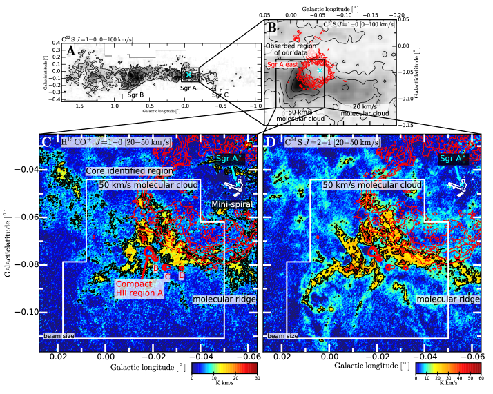
Figure 1: [A] Integrated intensity map of the CMZ in the ${\rm C^{32}S}~{}J=1-0$ emission line with contours (black solid line) (Tsuboi et al., 1999). The cyan cross shows the position of the Sgr A*. [B] Integrated intensity map of the ${\rm C^{32}S}~{}J=1-0$ emission line of the Sgr A region with contours (black solid line) (Tsuboi et al., 1999). Red contours show the 6cm continuum emission map (Yusef-Zadeh & Morris, 1987). The contour levels are $0.02,0.04,0.06$ and $0.08\rm~{}Jy~{}beam^{-1}$. The black thick line shows the region observed with ALMA. [C] Integrated intensity map of ${\rm H^{13}CO^{+}}~{}J=1-0$ with contours (black solid line) is shown as a guide map. The integration range is $V_{\rm LSR}=20-50\rm~{}km~{}s^{-1}$. The color bar shows the intensity range of $0-30\rm~{}K~{}km~{}s^{-1}$, and the contour levels are $10$ and $20\rm~{}K~{}km~{}s^{-1}$. White contours show the continuum emission map in the 100 GHz band of the mini-spiral observed by ALMA (Tsuboi et al., 2016). The contour levels are $0.01$ and $0.015\rm~{}Jy~{}beam^{-1}$. [D] Integrated intensity map of ${\rm C^{34}S}~{}J=2-1$ with contours (black solid line) is shown as a guide map. The integration range is $V_{\rm LSR}=20-50\rm~{}km~{}s^{-1}$. The color bar shows the intensity range of $0-60\rm~{}K~{}km~{}s^{-1}$, and the contour levels are $15,~{}30$ and $45\rm~{}K~{}km~{}s^{-1}$.

Table 1: The parameters of the ALMA observation

Source	G-0.02-0.07
Obs. region [$\rm arcsec^{2}$]	$330\times 330$
Mosaic pointing (12m array)	137 pointings
Mosaic pointing (7m array)	52 pointings
	${\rm H^{13}CO^{+}}~{}J=1-0$	${\rm C^{34}S}~{}J=2-1$
Rest frequency [GHz]	86.754	96.413
Angular resolution [$\rm arcsec^{2}$]	$2.04\times 1.41$	$2.00\times 1.35$
Physical resolution $[{\rm pc^{2}}]$ (@$8.5\rm~{}kpc$)	$\rm 0.083\times 0.058$	$0.082\times 0.056$
Peak intensity [K]	2.1	3.9
Conversion factor [$\rm K/(Jy~{}beam^{-1})$]	56.4	48.7
Peak velocity $[\rm km~{}s^{-1}]$	52	49
FWHM velocity width $[\rm km~{}s^{-1}]$	$34$	37

3 Channel maps of the ${\rm H^{13}CO^{+}}~{}J=1-0$ and ${\rm C^{34}S}~{}J=2-1$ emission lines

First of all, we evaluated how much the feathering method restores the missing flux of structures extending larger than the observable scale by ACA. Figure 2 shows the spectra of the ALMA feathering map, the ALMA interferometer map, and the NRO45 map. The flux density ratio of the ALMA interferometer map to the NRO45 map is $\sim 0.15$, whereas the ratio of the ALMA feathering map to the NRO45 map is as high as $\sim 0.8$. Considering the calibration error between the ALMA feathering map and NRO45 map, the feathering method restores the missing flux quite well. We use the missing flux restored maps by the feathering method hereafter in this paper.

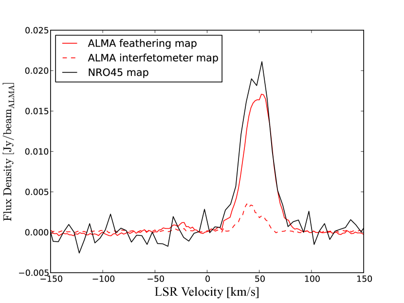
Figure 2: Spectra of the ALMA feathering ${\rm H^{13}CO^{+}}$ map (red solid line), the ALMA interferometer map (red dashed line), and the NRO45 map (black solid line). These spectra were calculated inside a circle with a radius of 30 arcsec, centered on the 50MC center of $(l,b)=(-0\fdg 02,-0\fdg 07)$. The intensity scales of the spectra are shown in the units of $\rm Jy/(2\farcs 04\times 1\farcs 41)$.

The channel maps of the ${\rm H^{13}CO^{+}}~{}J=1-0$ emission line are shown in Figure 3. These maps show the dense region of the 50MC because the H¹³CO${}^{+}~{}J=1-0$ emission line has a high critical density of $\sim 10^{5}\rm~{}cm^{-3}$. We show the velocity range of $0\rm~{}km~{}s^{-1}$ to $100\rm~{}km~{}s^{-1}$ in $V_{\rm LSR}$ because the 50MC is not detected out of this velocity range. In the same velocity range, the channel maps of the ${\rm C^{34}S}~{}J=2-1$ emission line also are shown in Figure 4. The positions of Sgr A* (white star) and four HII regions (white cross) are shown on each channel map.

The molecular ridge (e.g. Coil & Ho, 2000; Park et al., 2004) is seen in the velocity range of $V_{\rm LSR}=26-60\rm~{}km~{}s^{-1}$ to the west of the 50MC in both the ${\rm H^{13}CO^{+}}$ and ${\rm C^{34}S}$ maps. The bright components only in the ${\rm H^{13}CO^{+}}$ maps exist on $(l,b)=(-0\fdg 046,-0\fdg 056)$ with $V_{\rm LSR}=48-78\rm~{}km~{}s^{-1}$ which was observed in the ${\rm HCO^{+}}~{}J=1-0$ and HCN $J=1-0$ emission lines as the dense clumps (Christopher et al., 2005). The other bright components exist on $(l,b)=(-0\fdg 051,-0\fdg 056)$ with $V_{\rm LSR}=18-28\rm~{}km~{}s^{-1}$. The compact HII region D is found at $(l,b)=(-0\fdg 04,-0\fdg 08)$ by absorption in the maps of $V_{\rm LSR}=32-48\rm~{}km~{}s^{-1}$ in the ${\rm H^{13}CO^{+}}$ maps. These features are summarized in Figure 1-C.

These channel maps with $0.1\rm~{}pc$ resolution revealed that the 50MC has clumpy and filamentary structures as shown in Figure 3 and 4. The filamentary structures are conspicuous in the range of $30-40\rm~{}km~{}s^{-1}$ in $V_{\rm LSR}$ and radially extended from around the center of the 50MC in the ${\rm H^{13}CO^{+}}$ maps. On the other hand, in the ${\rm C^{34}S}$ maps, the filamentary structures can be confirmed more clearly compared with those in the ${\rm H^{13}CO^{+}}$ maps. The filamentary structures are apparent in the range of $24-40\rm~{}km~{}s^{-1}$ in $V_{\rm LSR}$ and radially extended from around the center of the 50MC. The filamentary structures are also found distinctly in the CS $J=2-1$ channel maps (Uehara et al., 2017). Filamentary structures in molecular clouds are found in the Galactic disk region (e.g. André et al., 2010) from the Herschel survey observations (Pilbratt et al., 2010). It has been revealed that the molecular clouds ubiquitously exist as filamentary structures in the Galactic disk region. On the other hand, the filamentary structures in the CMZ have been detected in G0.253$+$0.016 with ALMA (Rathborne et al., 2015), but other molecular clouds with filamentary structures have not yet been found in the CMZ. The existence of a number of the filamentary structures in the 50MC strongly suggests that the filamentary structures are also ubiquitous in the molecular clouds in the CMZ.

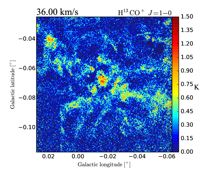
Figure 3: Channel maps with velocity widths of $2\rm~{}km~{}s^{-1}$ of the ${\rm H^{13}CO^{+}}~{}J=1-0$ emission line. The central velocity of each channel is shown in the upper left corner of each panel, which ranges from 0 to 100 $\rm km~{}s^{-1}$ in $V_{\rm LSR}$. Figure 3 is published in its entirety in http://www.vsop.isas.jaxa.jp/~nakahara/figure_uehara/201812/fig3.zip. The range of the brightness temperature $T_{\rm B}$ in the maps is $-28.4$ to $3.6\rm~{}K$. The color bars of the $T_{\rm B}$ are shown on the right side of the rightmost maps with the range of $0.0-1.5\rm~{}K$ because we do not consider the absorption at the Sgr A^∗ and H_II region D. The white star and white crosses show the position of the Sgr A* and four HII regions, respectively. The inset figures of each panel show the beam size. Additionally, we supply the channel map movie (http://www.vsop.isas.jaxa.jp/~nakahara/figure_uehara/201812/map_h13co+.mp4)

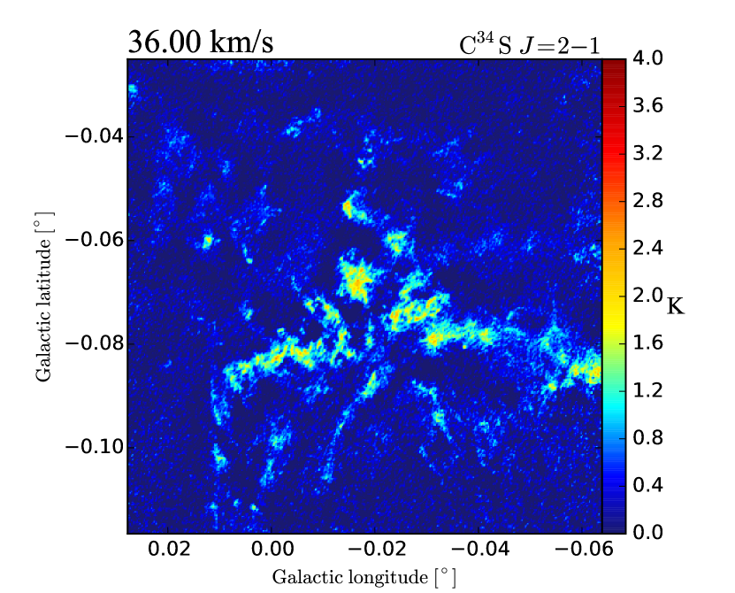
Figure 4: Channel maps with velocity widths of $2\rm~{}km~{}s^{-1}$ of the $\rm C^{34}S$ $J=2-1$ emission line. The central velocity of each channel is shown on the upper left corner of each panel, which ranges from 0 to 100 $\rm km~{}s^{-1}$ in $V_{\rm LSR}$. Figure 4 is published in its entirety in http://www.vsop.isas.jaxa.jp/~nakahara/figure_uehara/201812/fig4.zip. The range of the brightness temperature $T_{\rm B}$ in the maps is $-4.5$ to $4.0\rm~{}K$. The color bars of the $T_{\rm B}$ are shown on the right side of the rightmost maps with the range of $0.0-4.0\rm~{}K$ because we do not consider the absorption at the Sgr A^∗ and H_II region D. The white star and white crosses show the position of the Sgr A* and four HII regions, respectively. The inset figures of each panel show the beam size. We supply the channel map movie (http://www.vsop.isas.jaxa.jp/~nakahara/figure_uehara/201812/map_c34s.mp4)

4 Molecular Cloud Core Identification

4.1 Identification of the molecular cloud core candidates

We identified molecular cloud cores in the 3D ($l-b-v_{\rm LSR}$) H¹³CO${}^{+}~{}J=1-0$ and ${\rm C^{34}S}~{}J=2-1$ data with the velocity range of $0-100\rm~{}km~{}s^{-1}$ in $V_{\rm LSR}$ using the $clumpfind$ algorithm (Williams et al., 1994). The clumpfind algorithm finds local peaks as clumps in the data cube and does not determine whether those clumps are bound or not. Therefore, we refer to the identified clumps as core candidates in this section. Before the clumpfind was applied, the maps were resampled using a sample interval of $1\farcs 5\times 1\farcs 5$, which corresponds to the FWHM of the ALMA beam. We analyzed core candidates only within the white boundary line in Figure 1 in order to examine the core candidates in the 50MC. In the clumpfind algorithm, the parameters, Lowest contour level and Contour increment, were set to $2\sigma$ and $2\sigma$ corresponding to 0.32 K and 0.32 K, respectively. The original FWHM velocity width is calculated as

$$\Delta v=2\sqrt{2\ln 2}\left[\frac{\displaystyle\sum_{i}v_{i}^{2}T_{i}}{\displaystyle\sum_{i}T_{i}}-\left(\frac{\displaystyle\sum_{i}v_{i}T_{i}}{\displaystyle\sum_{i}T_{i}}\right)^{2}\right]^{1/2},$$ (1)

where $v_{i}$ and $T_{i}$ are the radial velocity and intensity of the $i$-th pixel in each core candidate, respectively. The FWHM velocity width $\Delta V_{\rm FWHM}$ is corrected for the velocity resolution by

$$\Delta V_{\rm FWHM}=\left(\Delta v^{2}-2{[\rm km~{}s^{-1}]}^{2}\right)^{1/2}.$$ (2)

The original radius of the core candidate is defined as the effective circular radius,

$$r=\left(\frac{A}{\pi}\right)^{1/2},$$ (3)

where $A$ is the projected area of each core candidate derived by the clumpfind. The beam-deconvolved radius $R$ of the core candidate is calculated by

$$R=\left[r^{2}-\left\{\frac{\sqrt{\theta_{\rm major}\times\theta_{\rm minor}}}{\sqrt{2\ln 2}}\left(2\ln\frac{T_{\rm peak}}{\Delta T}\right)^{1/2}\right\}^{2}\right]^{1/2},$$ (4)

where $T_{\rm peak}$, $\Delta T$, $\theta_{\rm major}$ and $\theta_{\rm minor}$ are the peak temperature in the core candidate, the threshold level in the core candidate identification, the beam semi major axis and the beam semi minor axis, respectively (Williams et al., 1994). The core candidates whose deconvolved radii are smaller than 0.035pc were rejected because the deconvolved radius is less than the mean beam radius of $\sqrt{\theta_{\rm major}\times\theta_{\rm minor}}/2$, $\sim 0.035\rm~{}pc$. Furthermore, we rejected the detected core candidates that do not have three or more pixels with intensities of $\geq 3\sigma$ or the core candidates that do not have two or more velocity channels. Finally, we identified 3293 core candidates in the ${\rm H^{13}CO^{+}}$ data and 3192 core candidates in the ${\rm C^{34}S}$ data, respectively. The number of the identified core candidates in these data is $\sim 100$ times larger than that in the previous work using the CS $J=1-0$ emission line (Tsuboi & Miyazaki, 2012). This number is also $\sim 15$ times larger than the number of the cores in the Orion A cloud identified by Ikeda et al. (2007). The large number seems enough for statistical analysis. Because our observation resolved the core candidates nearly to the minimum spatial scale, 0.06 pc, observed by existing single dish telescopes in the Orion A molecular cloud (Ikeda et al., 2007), it becomes possible to directly compare the core candidate properties in the 50MC and a typical Galactic disk molecular cloud, the Orion A cloud, as mentioned in §2. The core candidates are distributed throughout the 50MC.

4.2 Mass estimation of the core candidate

The physical parameters of the ${\rm H^{13}CO^{+}}$ and ${\rm C^{34}S}$ core candidates are estimated in this section and are summarized in Table 3 and 4, respectively.

Firstly, we calculate the column densities of the $\rm H^{13}CO^{+}~{}J=1-0$ and ${\rm C^{34}S}$ core candidates. From the total intensities of the H¹³CO${}^{+}~{}J=1-0$ and ${\rm C^{34}S}$ emission lines of the core candidates, $\int T_{\rm MB}dV[{\rm K~{}km/s}]$, the core candidate masses are estimated assuming the local thermodynamic equilibrium (LTE) condition. The $\rm H_{2}$ column densities of the ${\rm H^{13}CO^{+}}$ core candidates are estimated from the equation given by,

$$N_{\rm H_{2}}{\rm[cm^{-2}]}=\frac{2.53\times 10^{11}}{1-\exp(-4.16/T_{\rm ex,H^{13}CO^{+}})}\frac{\displaystyle\int T_{\rm MB}dV[{\rm K~{}km/s}]}{X({\rm H^{13}CO^{+}})}.$$ (5)

Here $T_{\rm ex,H^{13}CO^{+}}$ is the excitation temperature of the H¹³CO${}^{+}~{}J=1-0$ emission line; $X(\rm H^{13}CO^{+})$ is the fractional abundance, $X({\rm H^{13}CO^{+}})=N_{\rm H^{13}CO^{+}}/N_{\rm H_{2}}$, which is the relative abundance of H¹³CO⁺ molecules to total $\rm H_{2}$ molecules. The $X(\rm H^{13}CO^{+})$ is assumed to be $6\times 10^{-11}$ with uncertainty of a factor of 2 in the CMZ (Amo-Baladrón et al., 2011). Amo-Baladrón et al. (2011) estimated that the fractional abundances of other CMZ clouds are $X(\rm H^{13}CO^{+})=(5-25)\times 10^{-11}$, while those of the galactic disk clouds are $X(\rm H^{13}CO^{+})=(5-18)\times 10^{-11}$. It is similar to that in the Orion A of $4.8\times 10^{-11}$ (Ikeda et al., 2007). On the other hand, the $\rm H_{2}$ column densities of the ${\rm C^{34}S}$ core candidates are estimated from the equation given by,

$$N_{\rm H_{2}}{\rm[cm^{-2}]}=9.03\times 10^{11}\frac{\exp(2.31/T_{\rm ex,C^{34}S})}{1-\exp(-4.63/T_{\rm ex,C^{34}S})}\frac{\displaystyle\int T_{\rm MB}dV[{\rm K~{}km/s}]}{X({\rm C^{34}S})}.$$ (6)

Here $T_{\rm ex,C^{34}S}$ is the excitation temperature of the ${\rm C^{34}S}~{}J=2-1$ emission line; the fractional abundance $X(\rm{\rm C^{34}S})$ is assumed to be $4.87\times 10^{-10}$ (Amo-Baladrón et al., 2011). For the Orion A cloud, Ungerechts et al. (1997) derived $[{\rm C^{32}S}]/[{\rm{}^{12}CO}]=(0.5-2)\times 10^{-4}$. Using $[{\rm{}^{12}CO}]/[{\rm H_{2}}]=6.0\times 10^{-5}$ (Frerking et al., 1982; Savage et al., 2002) and $\rm[^{32}S]/[^{34}S]=22.4$, a fractional abundance is estimated to be $X(\rm{\rm C^{34}S})=(1.3-5.3)\times 10^{-10}$ in the Orion A. This value is consistent with that in the 50MC.

Using the RADEX LVG (Large Velocity Gradient) algorithm (van der Tak et al., 2007), we estimated the $T_{\rm ex}$ from the ${\rm C^{32}S}~{}J=1-0$ (NMA: Tsuboi et al., 2009) and $2-1$ (our ACA+TP data) emission line data within the circle with 78 arcsec radius centered on the 50MC center (the field of view of the NMA). The results of the LVG analysis are shown in Figure 5. The black thick lines and the red thick lines show the brightness temperature, $T_{\rm B}({\rm C^{32}S}~{}J=2-1)$, and the brightness temperature ratio, $T_{\rm B}({\rm C^{32}S}~{}J=2-1)/T_{\rm B}({\rm C^{32}S}~{}J=1-0)$, respectively. The core candidates identified by the ${\rm H^{13}CO^{+}}$ (panel A) and ${\rm C^{34}S}$ (panel B) observations are plotted on the LVG diagrams as the colored filled circles. The colors of the plotted circles indicate the excitation temperature of the ${\rm C^{32}S}~{}J=2-1$ transition in each core candidate. Because the $T_{\rm ex}$ scatters in the wide range of $5-150\rm~{}K$ for both the ${\rm H^{13}CO^{+}}$ and ${\rm C^{34}S}$ core candidates, we used the $T_{\rm ex}$ obtained for each core candidate in the column density estimation.

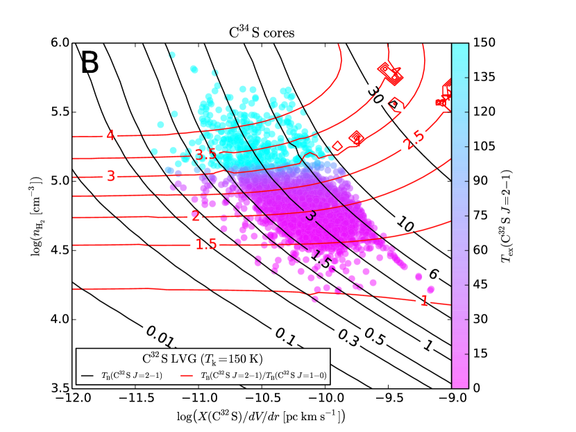
Figure 5: Curves of the brightness temperature $T_{\rm B}({\rm C^{32}S}~{}J=2-1)$ (black lines) and the intensity ratio $T_{\rm B}({\rm C^{32}S}~{}J=2-1)/T_{\rm B}({\rm C^{32}S}~{}J=1-0)$ (red lines) are shown on the planes of $\rm H_{2}$ number density vs. CS fractional abundance per velocity gradient. [A] The colored filled circles show the observed data of the ${\rm H^{13}CO^{+}}$ core candidates. The color bar shows the excitation temperature of each ${\rm H^{13}CO^{+}}$ core candidates. [B] The colored filled circles show the observed data of the ${\rm C^{34}S}$ core candidate. The color bar shows the excitation temperature of each ${\rm C^{34}S}$ core candidate.

Finally, we calculate the core candidate masses from the equation given by,

$$M[M_{\odot}]=\mu[M_{\odot}]\sum_{m}\sum_{n}\left(N_{\rm H_{2}}(m,n){\rm[cm^{-2}]}\Omega[{\rm cm^{2}}]\right).$$ (7)

The summation is done over each core candidate area. Here $\Omega$ is the physical area of a pixel of the map; $\mu$ is the mean mass of the molecular gas per $\rm H_{2}$ molecule. These values are $\Omega=3.64\times 10^{34}\rm cm^{2}$ for the $1\farcs 5$ pixel size at the 8.5 kpc distance and $\mu=2.35\times 10^{-57}M_{\odot}$. We also estimate the mass detection limit in our identification. According to our identification, at least 3 pixels of $3\sigma=0.48\rm~{}K$ or more are included in a core. Since the $T_{\rm ex}$ obtained by the LVG analysis is $5-150\rm~{}K$, the mass detection limit is estimated to be $0.6-13~{}M_{\odot}$ using equation 5-7. Thus, the detection limit of the ${\rm H^{13}CO^{+}}$ core mass comes to be $0.6~{}M_{\odot}$. Similarly, the detection limit of the ${\rm C^{34}S}$ core mass is estimated to be $0.4~{}M_{\odot}$.

The average and range of the ${\rm H^{13}CO^{+}}$ core candidate masses are $(2.3\pm 3.7)\times 10^{2}M_{\odot}$ and $4.3-4500M_{\odot}$, respectively (See the column 9 in Table 3). The total core candidate mass is estimated to be $7.6\times 10^{5}M_{\odot}$. The total LTE mass of the 50MC is $1.3\times 10^{6}M_{\odot}$ from the H¹³CO${}^{+}~{}J=1-0$ channel maps with the velocity range of $0-100\rm~{}km~{}s^{-1}$ in $V_{\rm LSR}$. Thus, the ratio of the total core candidate mass to the mass of the whole of the 50MC is $58\%$ ($=7.6\times 10^{5}M_{\odot}/1.3\times 10^{6}M_{\odot}$).

The average and range of the ${\rm C^{34}S}$ core candidate masses also are $(1.9\pm 3.6)\times 10^{2}M_{\odot}$ and $2.4-5500M_{\odot}$, respectively (See the column 9 in Table 4). The total mass of the core candidate is estimated to be $6.1\times 10^{5}~{}M_{\odot}$. The total LTE mass of the 50MC is $7.3\times 10^{5}~{}M_{\odot}$ from the ${\rm C^{34}S}~{}J=2-1$ channel maps with the velocity range of $0-100\rm~{}km~{}s^{-1}$ in $V_{\rm LSR}$. Thus, the mass ratio of the core candidates to the whole 50MC is $83\%$ ($=6.1\times 10^{5}~{}M_{\odot}/7.3\times 10^{5}~{}M_{\odot}$). The total LTE mass of the 50MC is smaller than that derived from the ${\rm H^{13}CO^{+}}~{}J=1-0$ maps as estimated above. Because the uncertainty of the abundance that is used to estimate the mass is up to a factor of 2 (Amo-Baladrón et al., 2011), the two masses coincide within the uncertainties.

Additionally, assuming a sphere shape with radius $R$, the mean number density of the core candidate, $\overline{n}$, is given by

$$\overline{n}~{}[{\rm cm^{-3}}]=\frac{3M_{\rm LTE}[M_{\odot}]}{4\pi\mu[M_{\odot}]R[{\rm cm}]^{3}}.$$ (8)

These values are summarized in the column 11 in Table 3 and 4. The average and range of the $\overline{n}$ are $(1.7\pm 2.0)\times 10^{5}~{}{\rm cm^{-3}}$ and $(0.10-25)\times 10^{5}~{}{\rm cm^{-3}}$ for the ${\rm H^{13}CO^{+}}$ core candidate, respectively. The $\overline{n}$ values are comparable to the critical number density of the H¹³CO${}^{+}~{}J=1-0$ emission line of $\sim 10^{5}~{}\rm cm^{-3}$. For the ${\rm C^{34}S}$ core candidates, the average and range of the densities $\overline{n}$ are $(1.0\pm 1.4)\times 10^{5}~{}{\rm cm^{-3}}$ and $(0.05-15)\times 10^{5}~{}{\rm cm^{-3}}$, respectively. The $\overline{n}$ values are also comparable to the critical number density of the ${\rm C^{34}S}~{}J=2-1$ emission line of $\sim 10^{5}~{}\rm cm^{-3}$.

We estimate the virial masses of the core candidates assuming no external pressure and no magnetic field. The virial masses are calculated by the equation

$$M_{\rm vir}[M_{\odot}] = 5R[{\rm pc}]\sigma[{\rm km~{}s^{-1}}]^{2}/G$$ (9)

$$= 210\times R[{\rm pc}]\Delta V_{\rm FWHM}[\rm km~{}s^{-1}]^{2},$$ (10)

where $\sigma$ and $\Delta V_{\rm FWHM}[\rm km~{}s^{-1}]$ are the velocity dispersion and the FWHM velocity width of the core candidate, respectively (see the column 6 and 8 in the Table 3 and 4). The average and range of the virial masses are $(17.9\pm 15.3)\times 10^{2}M_{\odot}$ and $(0.83-228)\times 10^{2}M_{\odot}$ for the ${\rm H^{13}CO^{+}}$ core candidates, respectively. Those of the ${\rm C^{34}S}$ core candidates are $(18.8\pm 13.6)\times 10^{2}M_{\odot}$ and $(0.76-137)\times 10^{2}M_{\odot}$, respectively.

In addition, the virial parameters defined by the ratio of the virial mass and the LTE mass ($\alpha=M_{\rm vir}/M_{\rm LTE}$) are calculated. The large $\alpha$ ($>1$) indicates that the core candidate is unbound by self-gravity, whereas the small $\alpha$ ($<1$) indicates that the core candidate is bound by self-gravity. These values are summarized in the column 10 in Table 3 and 4. For the ${\rm H^{13}CO^{+}}$ core candidates, the average and range of the virial parameter are $19\pm 25$ and $0.40-450$, respectively. These values of the ${\rm C^{34}S}$ core candidates are $38\pm 52$ and $0.8-810$, respectively. The virial parameter in the 50MC is two to three orders of magnitude larger than that in the Orion A (Ikeda et al., 2007) and is also larger than that of the whole of the 50MC ($\alpha\sim 2$) (Tsuboi et al., 2011). They suggest that the gas in the core candidates is strongly turbulent and are often unbound by self-gravity.

5 Discussion

5.1 Identification of Bound cores

Because the range of the virial parameters of the cores in the Orion A is 0.2-4, almost all of the cores are likely to be bound by self-gravity (Ikeda et al., 2007). On the other hand, the virial parameters in the 50MC scatter in the range of 0.4-810 (§4.2), indicating a mixture of bound and unbound cores. The criterion for the bound cores is nominally that the virial parameter is less than unity. Because the uncertainty of the fractional abundance of $X({\rm H^{13}CO^{+}})$ is as large as a factor of 2 (Amo-Baladrón et al., 2011), the ${\rm H^{13}CO^{+}}$ core candidate mass may be underestimated down to a factor of 0.5. Therefore, we consider the ${\rm H^{13}CO^{+}}$ core candidates with the virial parameters of less than 2 as ”bound cores”. Additionally, in the previous works (e.g. Ikeda et al., 2007, 2009), the cores identified by the clumpfind have the radii of $\sim 0.1\rm~{}pc$. The radii of the bound ${\rm H^{13}CO^{+}}$ cores in the 50MC are comparable to those in the previous works. The 241 bound cores were identified. The number corresponds to $7\%~{}(=241/3293)$ of all the identified core candidates. The positions of the bound cores are shown in Figure 6-A. Thus, we use only the bound cores in the CMF analysis hereafter in order to compare the cores between the 50MC and the Orion A. Meanwhile, the bound ${\rm C^{34}S}$ cores with $\alpha<2$ ($\sim 4\%=129/3192$ of all the identified ${\rm C^{34}S}$ core candidates) are plotted in Figure 6-B (the uncertainty in $X({\rm C^{34}S})$ is also a factor of $\sim 2$). The physical parameters of the bound ${\rm H^{13}CO^{+}}$ and ${\rm C^{34}S}$ cores are summarized in Table 5. On the other hand, we call the core candidates with $\alpha>2$ ”transient cores”.

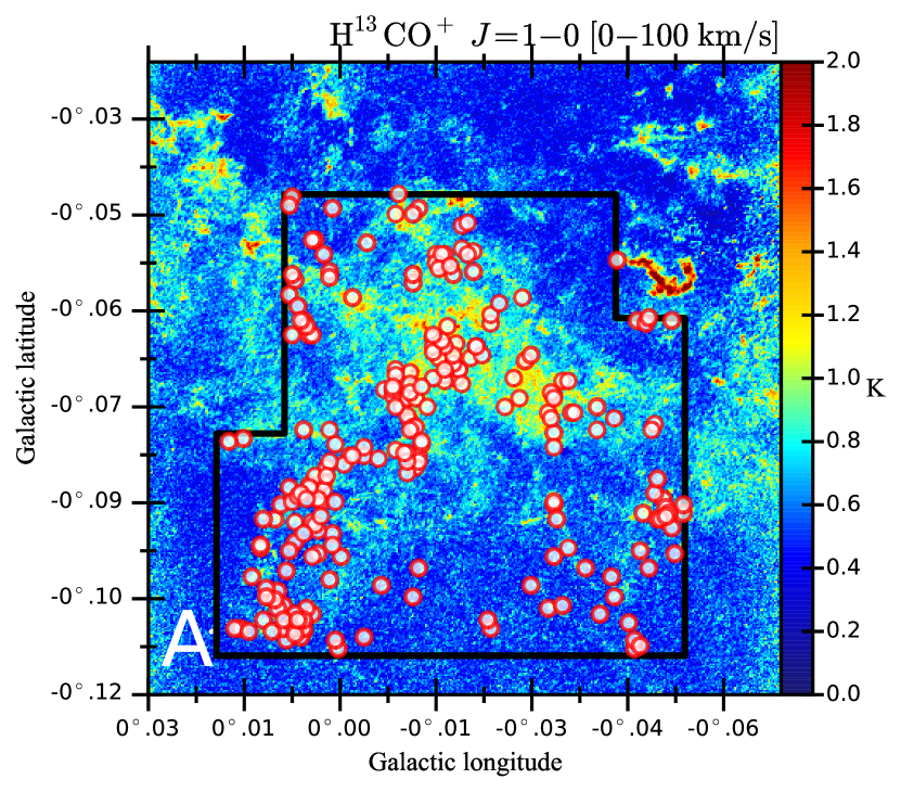
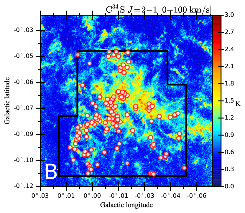
Figure 6: [A] Positions of the identified bound ${\rm H^{13}CO^{+}}$ cores with $\alpha<2$ on the $T_{\rm peak}$ map of the ${\rm H^{13}CO^{+}}~{}J=1-0$ emission line in the units of brightness temperature ($\rm K$) over the velocity range of $V_{\rm LSR}=0-100\rm~{}km~{}s^{-1}$. The cores outside the polygon with the black thick line are rejected. [B] Positions of the identified bound ${\rm C^{34}S}$ cores with $\alpha<2$ on the $T_{\rm peak}$ map of the ${\rm C^{34}S}J=2-1$ emission line in the units of brightness temperature ($\rm K$) over the velocity range of $V_{\rm LSR}=0-100\rm~{}km~{}s^{-1}$. The cores outside the polygon with the black thick line are rejected.

Figure 7 shows the bound cores identified in both the ${\rm H^{13}CO^{+}}~{}J=1-0$ and ${\rm C^{34}S}~{}J=2-1$ emission lines. We regard the bound cores that satisfy the following two criteria as the identification by the both lines:

1. The distance between the centers of the $\rm C^{34}S$ and $\rm H^{13}CO^{+}$ cores is smaller than the larger radius of the two cores.

2. The difference between the center LSR velocities of the $\rm C^{34}S$ and $\rm H^{13}CO^{+}$ cores is smaller than the larger velocity width of the two cores.

Finally, $38~{}\%~{}(=49/129)$ of ${\rm C^{34}S}$ bound cores are found to have the ${\rm H^{13}CO^{+}}$ counterparts.

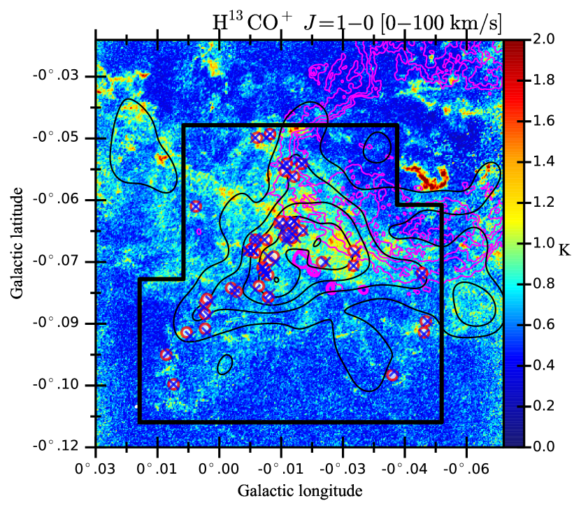
Figure 7: [A] Bound cores identified in both the ${\rm H^{13}CO^{+}}~{}J=1-0$ (blue cross) and ${\rm C^{34}S}~{}J=2-1$ (red open circle) emission lines plotted on the same ${\rm H^{13}CO^{+}}$ map as in Figure 6. Red contours show the H42$\alpha$ recombination line. Black contours show the $R_{T}=T_{\rm B}({\rm SiO}~{}J=2-1)/T_{\rm B}({\rm H^{13}CO^{+}}~{}J=1-0)$ smoothed to $26^{\prime\prime}$ resolution. The contour levels are 1.4,2.5,3.6,4.7 and 5.8.

5.2 Relation between the bound and transient cores

We compare the physical parameters of the bound and transient cores to understand the formation process of the bound cores. Note that the massive bound cores with greater than $\sim 1000~{}M_{\odot}$ might be precursors of stellar clusters. The average and range of the bound ${\rm H^{13}CO^{+}}$ core LTE masses, $M_{\rm LTE}$, are $960\pm 850~{}M_{\odot}$ and $48-4500\rm~{}M_{\odot}$, respectively. The core with the smallest mass of $48~{}M_{\odot}$ is larger than the detection limit of the ${\rm H^{13}CO^{+}}$ core mass; the mass detection limit is $13~{}M_{\odot}$ at $T_{\rm ex,{\rm H^{13}CO^{+}}}=150\rm~{}K$. On the other hand, the average and range of the ${\rm H^{13}CO^{+}}$ transient core LTE masses are $170\pm 210~{}M_{\odot}$ and $4.3-2000\rm~{}M_{\odot}$, respectively. The average and range of the bound core masses seem to be larger than those of the transient cores. Figure 8-A shows the cumulative distribution functions (CDFs) for the LTE masses of the bound (red line) and transient (black line) ${\rm H^{13}CO^{+}}$ cores. The mass distribution of the bound ${\rm H^{13}CO^{+}}$ cores is also biased to a larger mass than that of the transient ${\rm H^{13}CO^{+}}$ cores. The mass ratio of the total bound core mass to the total gas mass is $18~{}\%(=2.3\times 10^{5}~{}M_{\sun}/1.3\times 10^{6}~{}M_{\sun})$. The low mass ratio is consistent with the lower star formation rate in the CMZ, $\sim 0.1~{}M_{\odot}\rm~{}yr^{-1}$ (e.g. Güsten, 1989; Yusef-Zadeh et al., 2009; Barnes et al., 2017), than that in the disk region, $\sim 2.0~{}M_{\odot}\rm~{}yr^{-1}$ (e.g. Chomiuk & Povich, 2011).

Figure 9-A shows the CDFs for the virial masses of the bound (red line) and transient (black line) ${\rm H^{13}CO^{+}}$ cores. The average and range of the bound and transient core virial masses are indicated in Figure 9-A. The average and range of the bound cores are consistent with those of the transient cores within the uncertainties, respectively. However, the virial mass distribution of the bound ${\rm H^{13}CO^{+}}$ cores seems to be biased to a slightly smaller value than that of the transient ${\rm H^{13}CO^{+}}$ cores as shown in Figure 9-A.

The mean velocity widths of the bound and transient ${\rm H^{13}CO^{+}}$ cores are $5.4\pm 1.8\rm~{}km~{}s^{-1}$ and $6.8\pm 2.1\rm~{}km~{}s^{-1}$, respectively. In addition, the velocity width ranges of the bound and transient ${\rm H^{13}CO^{+}}$ cores are $2.1-11\rm~{}km~{}s^{-1}$ and $2.2-22\rm~{}km~{}s^{-1}$, respectively. The mean velocity width of the bound cores is consistent with that of the transient cores within the uncertainties. However, Figure 10-A shows the CDF for the velocity widths of the bound (red line) and transient (black line) ${\rm H^{13}CO^{+}}$ cores, indicating that the velocity width distribution of the bound cores is biased to a smaller velocity width than that of the transient cores.

Figure 11-A shows the CDFs for the radii of the bound (red line) and transient (black line) ${\rm H^{13}CO^{+}}$ cores. The average and range of the bound and transient ${\rm H^{13}CO^{+}}$ cores radii are shown in Figure 11-A. The mean radius of the bound cores is consistent with that of the transient cores within the uncertainties. On the other hand, the mean and range of the radii of the cores in the Orion A cloud are $0.14\pm 0.03\rm~{}pc$ and $0.06-0.23\rm~{}pc$, respectively, which are similar to those of the bound cores in 50MC. The radius distribution of the bound cores seems to be slightly larger than that of the transient cores as shown in Figure 11-A.

As shown above, the smaller velocity widths of the bound ${\rm H^{13}CO^{+}}$ cores make them bound by self-gravity, compared to the larger widths of the unbound cores. The mean radius ratio of the bound and transient ${\rm H^{13}CO^{+}}$ cores is $1.1$ and the velocity width ratio is $0.8$. From these ratios, the mean virial mass of the bound ${\rm H^{13}CO^{+}}$ cores are $1.1\times 0.8^{2}=0.7$ times smaller than that of the transient ${\rm H^{13}CO^{+}}$ cores because the virial mass is proportional to the radius and the square of the velocity width. Additionally, the small virial parameters of the bound ${\rm H^{13}CO^{+}}$ cores also depend on the distribution of the LTE masses biased to the large-mass side.

On the other hand, the bound ${\rm C^{34}S}$ cores have the larger LTE masses than the transient ${\rm C^{34}S}$ cores (see Figure 8-B) although the virial masses of the bound ${\rm C^{34}S}$ cores are consistent with those of the transient ${\rm C^{34}S}$ cores shown in Figure 9-B. The core with the smallest mass of $48~{}M_{\odot}$ is larger than the detection limit of the ${\rm C^{34}S}$ core mass; the mass detection limit is $5~{}M_{\odot}$ at $T_{\rm ex,{\rm C^{34}S}}=150\rm~{}K$. The mass ratio of the total bound core mass to the total gas mass is $23~{}\%(=1.7\times 10^{5}~{}M_{\sun}/7.3\times 10^{5}~{}M_{\sun})$. Additionally, the bound ${\rm C^{34}S}$ cores have the larger radii than the transient ${\rm C^{34}S}$ cores (see Figure 11-B) although the velocity widths of the bound ${\rm C^{34}S}$ cores are consistent with those of the transient ${\rm C^{34}S}$ cores (see Figure 10-B). The mean radius ratio of the bound and unbound ${\rm C^{34}S}$ cores is 1.29, and the velocity width ratio is 0.84. From these ratios, the mean virial masses of the bound and unbound ${\rm C^{34}S}$ cores are not different from each other because the mean virial mass of the bound ${\rm C^{34}S}$ cores is $1.29\times 0.84^{2}=0.92$ times smaller than that of the unbound ${\rm C^{34}S}$ cores. Thus, because the virial masses distribution of the bound ${\rm C^{34}S}$ cores is consistent with that of the transient cores, the ${\rm C^{34}S}$ cores need to have large masses in order for the virial parameter to be smaller than 2.

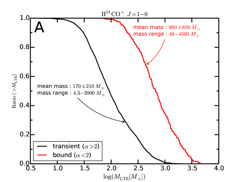
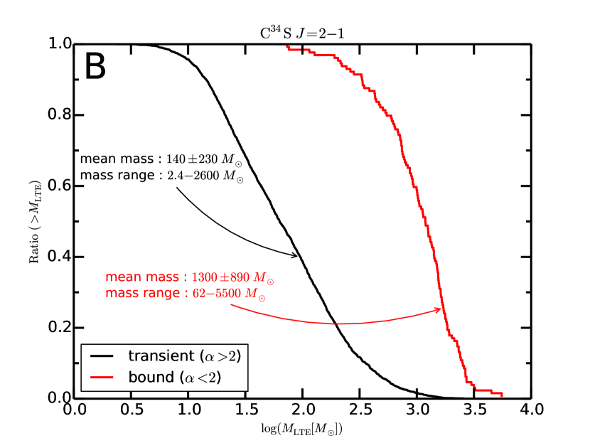
Figure 8: [A] CDF of the ${\rm H^{13}CO^{+}}~{}J=1-0$ core mass. The black thick line shows the distribution of the transient cores with $\alpha>2$, while the red thick line shows the distribution of the bound cores with $\alpha<2$. [B] CDF of the ${\rm C^{34}S}~{}J=2-1$ core mass.

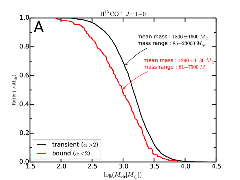
Figure 9: [A] CDF of the ${\rm H^{13}CO^{+}}~{}J=1-0$ core virial mass. The black thick line shows the distribution of the transient cores with $\alpha>2$, while the red thick line shows the distribution of the bound cores with $\alpha<2$. [B] CDF of the ${\rm C^{34}S}~{}J=2-1$ core virial mass.

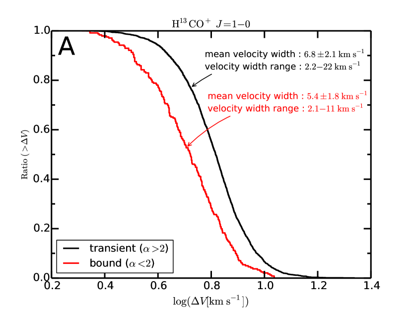
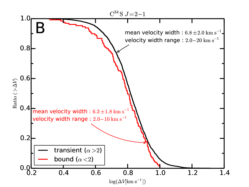
Figure 10: [A] CDF of the ${\rm H^{13}CO^{+}}~{}J=1-0$ core velocity width. The black thick line shows the distribution of the transient cores with $\alpha>2$, while the red thick line shows the distribution of the bound cores with $\alpha<2$. [B] CDF of the ${\rm C^{34}S}~{}J=2-1$ core velocity width.

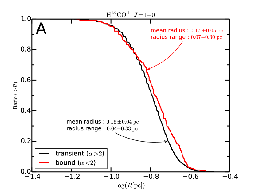
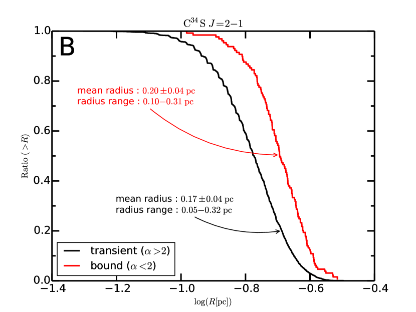
Figure 11: [A] CDF of the ${\rm H^{13}CO^{+}}~{}J=1-0$ core radii. The black thick line shows the distribution of the transient cores with $\alpha>2$, while the red thick line shows the distribution of the bound cores with $\alpha<2$. [B] CDF of the ${\rm C^{34}S}~{}J=2-1$ core radii.

5.3 Comparison of the bound cores in the 50MC and Orion A

The spatial resolution of our data, $\sim 0.07\rm~{}pc$, is similar to that in the Orion A observed by the NRO45 (e.g. $\sim 0.05\rm~{}pc$; Ikeda et al., 2007). Therefore, we can compare directly massive star forming processes in the GC 50MC and the typical Galactic disk molecular cloud, the Orion A cloud.

Firstly, most of the ${\rm H^{13}CO^{+}}$ core candidates in the 50MC ($\sim 93\%=3052/3293$) have $\sim 10-100$ times larger virial parameters than those in the Orion A (Ikeda et al., 2007) and are unbound only by self-gravity. Similarly, most of the ${\rm C^{34}S}$ core candidates ($\sim 96\%=3063/3192$) have $\sim 10-100$ times larger virial parameters than those in the Orion A. Thus, some external pressure is needed for confinement of the unbound core candidates. The core candidates are probably embedded in the ambient gas that is observed in lower critical density lines such as the ${\rm CO}~{}J=1-0$ and ${\rm CS}~{}J=1-0$ emission lines. If the ambient gas has low density but is highly turbulent, the core candidates may be bound by the external pressure of the gas. In this paper, note that the core candidates with $\alpha>2$ are treated as transient cores (probably pressure-confined cores) which we will discuss in a future paper.

Figure 12 shows the radius-velocity width relation of the dense cores ($R$-$\Delta V$ relation). The velocity widths of the bound cores in the 50MC are 10 times larger than those of the cores in the Orion A cloud. However, the radii of the bound cores detected in the 50MC are similar to those of the cores in the Orion A cloud.

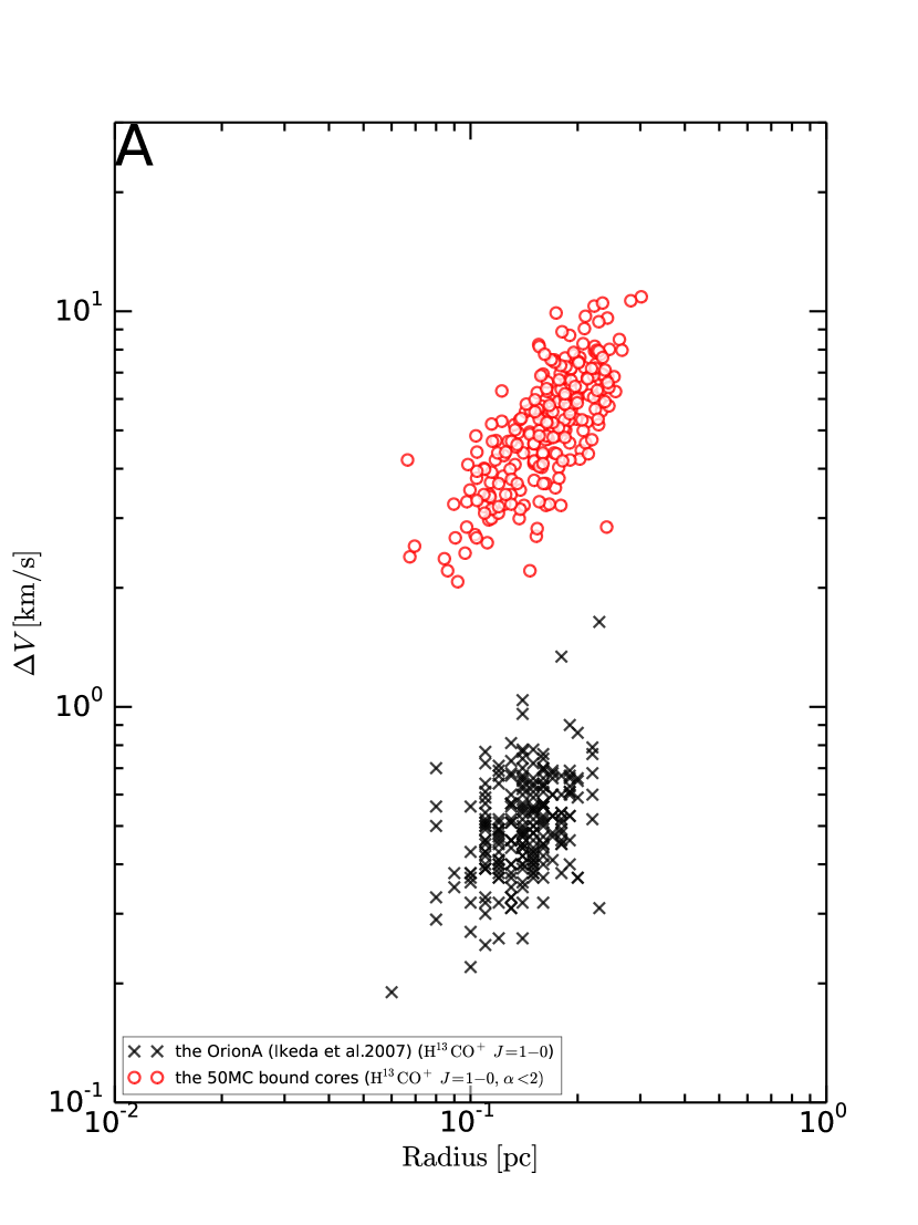
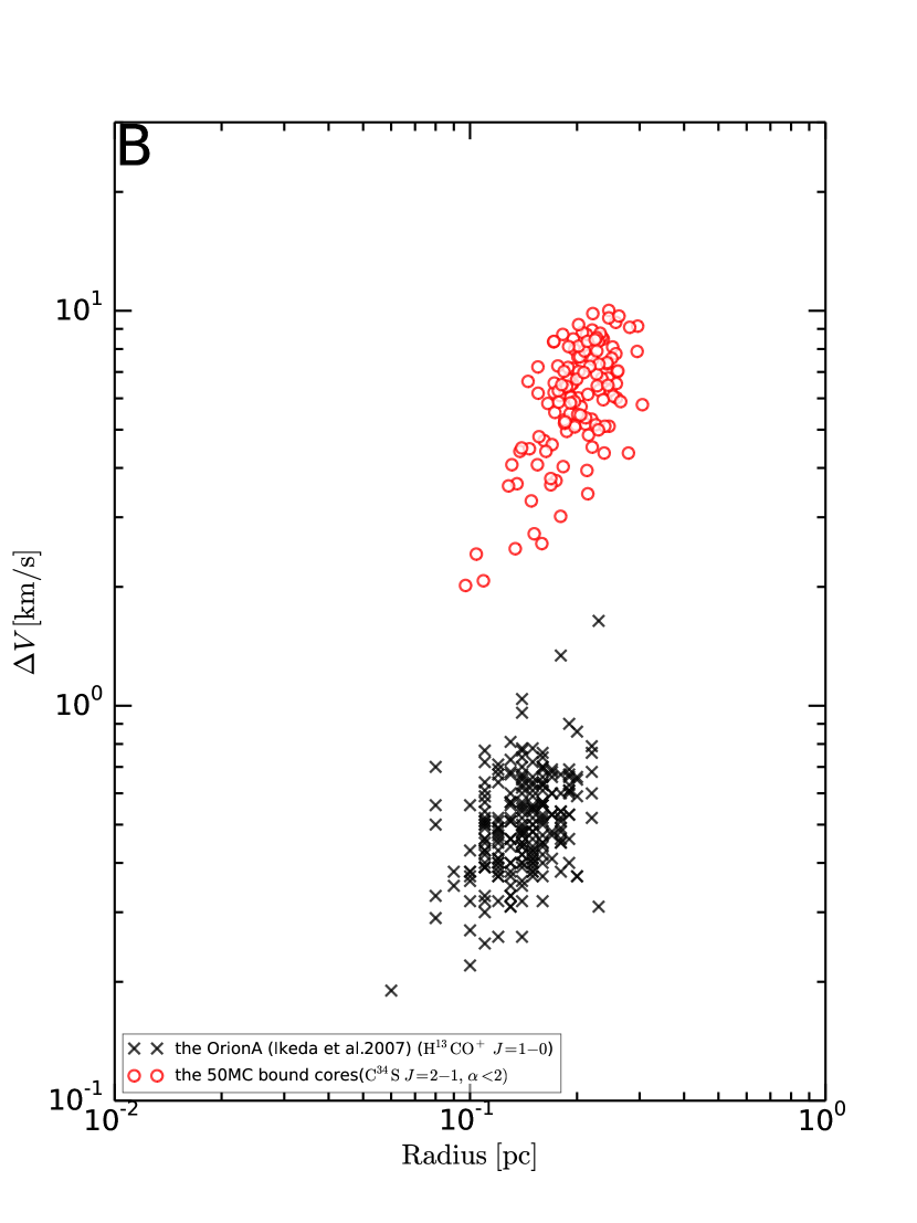
Figure 12: [A] Radius-velocity width relation of the ${\rm H^{13}CO^{+}}$ cores. [B] Radius-velocity width relation of the ${\rm C^{34}S}$ cores. The red circles show the bound cores in the 50MC. The black squares show the cores in the Orion A (Ikeda et al., 2007).

Figure 13-A shows the histograms of the LTE masses of the bound ${\rm H^{13}CO^{+}}$ cores in the 50MC (red bar) and the Orion A (black bar). The cores in the 50MC and the Orion A have different mass distributions. The mean mass in the Orion A is $12.3\pm 12.0~{}M_{\odot}$, whereas the mean mass in the 50MC is $960\pm 850M_{\odot}$ which is $\sim 80$ times larger than that in the Orion A.

The CMF of the bound ${\rm H^{13}CO^{+}}$ cores in the whole of the 50MC is shown in the Figure 13-B (red circle). For comparison, Figure 13-B also shows the CMF in the Orion A molecular cloud (black square) observed by the H¹³CO${}^{+}~{}J=1-0$ emission line (Ikeda et al., 2007). The CMF distributions in the 50MC and the Orion A are quite different from each other (also see Figure 13-A). Because the CMF of the 50MC becomes flat below $\sim 450~{}M_{\odot}$ which is larger than the detection limit of the ${\rm H^{13}CO^{+}}$ core mass of $13~{}M_{\odot}$ at $T_{\rm ex,{\rm H^{13}CO^{+}}}=150\rm~{}K$, we analyze the CMF in the 50MC above $400~{}M_{\odot}$ by using a usual single power-law function given by

$$\frac{dN}{dM}\propto M^{-\alpha_{\rm cmf}}.$$ (11)

Here $dN$ is the number of the cores whose masses are in the range of $M$ to $M+dM$; $\alpha_{\rm cmf}$ is the power-law index. The best-fit $\alpha_{\rm cmf}$ value is $1.48\pm 0.14$, which is smaller than that of $2.3\pm 0.1$ in the Orion A (Ikeda et al., 2007). Therefore, the CMFs of the bound ${\rm H^{13}CO^{+}}$ in the 50MC have a top-heavy distribution compared with those in the Orion A and in the previous work (Tsuboi et al., 2015).

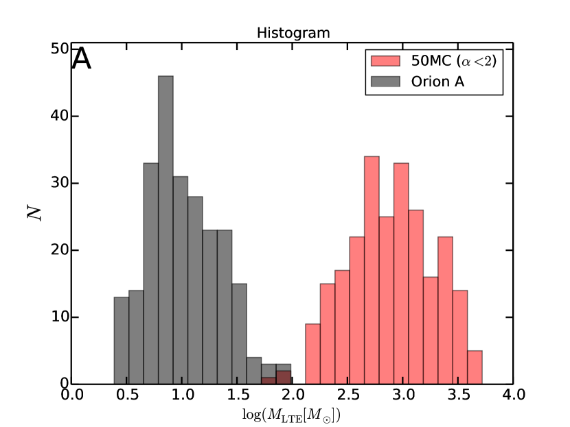
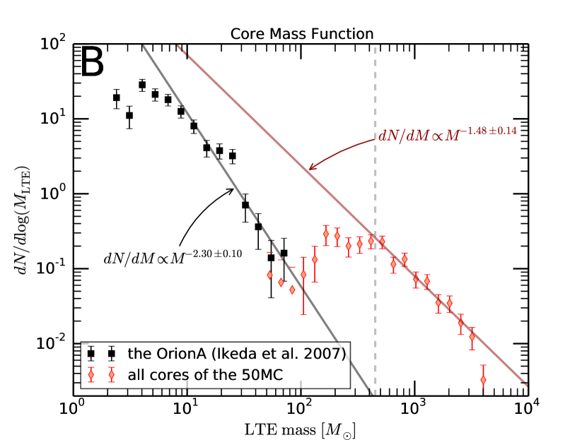
Figure 13: (A) Histogram of the bound ${\rm H^{13}CO^{+}}$ core mass in the 50MC (blue bars) and that of the Orion A cloud (black bars). (B) Core mass function of the 50MC bound cores (red circles) with the best-fitted single power-law line (red solid line). The power-law index is $1.48\pm 0.14$. The vertical gray dashed line shows $M_{\rm LTE}=450M_{\odot}$ and we analyze the CMF of the 50MC in the range of $>450M_{\odot}$. The core mass function of the Orion A cloud is shown by the black squares (Ikeda et al., 2007) with the best-fitted single power-law line (black solid line).

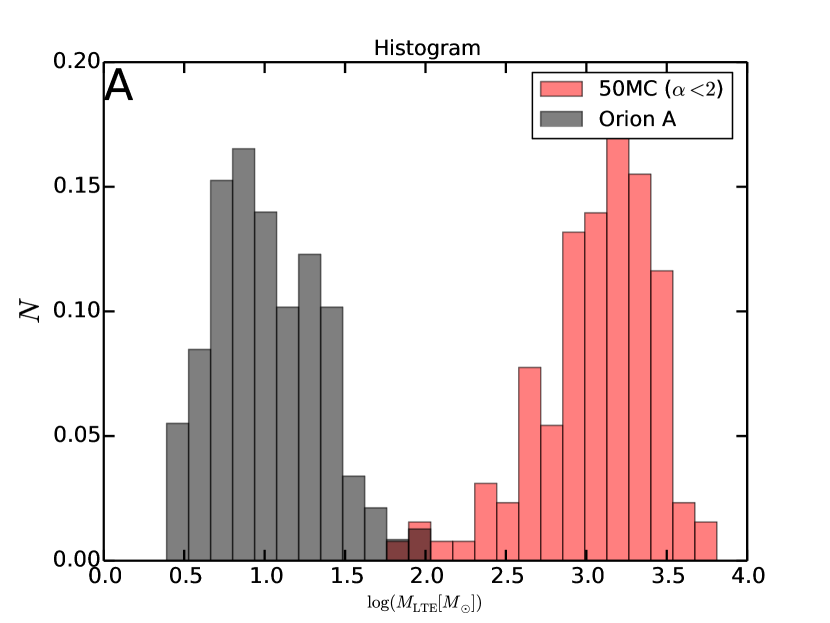
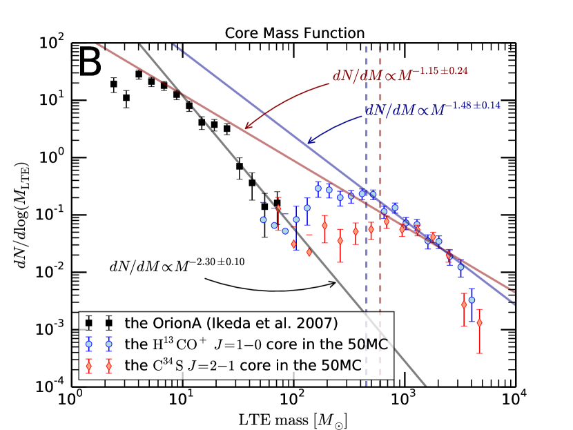
Figure 14: (A) Histogram of the bound ${\rm C^{34}S}$ core mass in the 50MC (blue bars) and that of the Orion A cloud (black bars). (B) Core mass function of the bound ${\rm C^{34}S}$ cores in the 50MC (red circles) with the best-fitted single power-law line (red solid line). The power-law index is $1.15\pm 0.24$. The vertical red dashed line shows $M_{\rm LTE}=600M_{\odot}$ and we analyze the CMF of the bound ${\rm C^{34}S}$ cores in the range of $>600M_{\odot}$. The blue circles indicate the CMF of the bound ${\rm H^{13}CO^{+}}$ cores. The blue circle and red solid line are the CMF and best-fitted single power-law line of the bound ${\rm H^{13}CO^{+}}$ cores, respectively. The CMF of the Orion A cloud is shown by the black squares (Ikeda et al., 2007) with the best-fitted single power-law line (black solid line).

We also make the CMF of the bound ${\rm C^{34}S}$ cores with $\alpha<2$. The mean mass of the bound cores is $1300\pm 890~{}M_{\odot}$ which is $\sim 100$ times larger than that in the Orion A (see Figure 14-A). Figure 14-B shows the CMFs of the bound ${\rm C^{34}S}$ and ${\rm H^{13}CO^{+}}$ cores for comparison. We applied a single power-law function to the CMF of the bound ${\rm C^{34}S}$ cores in the mass range from $600~{}M_{\odot}$ to $2000~{}M_{\odot}$. The best-fit $\alpha_{\rm cmf}$ value is $1.15\pm 0.24$. The power-law index of the bound ${\rm C^{34}S}$ cores is consistent with that of the bound ${\rm H^{13}CO^{+}}$ cores within the uncertainties.

Therefore, we conclude that the bound cores in the 50MC have a top-heavy mass distribution compared with those in the Orion A.

5.4 The bound cores in the CCC region

In this section, we discuss the influence of the CCC on the bound cores in terms of massive star formation.

5.4.1 The CCC in the 50MC

Tsuboi et al. (2015) found the half-shell-like shock structure with the brightness temperature ratio $R_{T}=T_{\rm B}({\rm SiO}~{}J=2-1)/T_{\rm B}({\rm H^{13}CO^{+}}~{}J=1-0)$ higher than 4 in the $l-b-v$ space observed by the NRO45. The $R_{T}$ is used as a shock tracer because the abundance of SiO molecules is increased by C-shock in molecular clouds, while the H¹³CO⁺ molecules are not affected by the shock (e.g. Amo-Baladrón et al., 2011). This shock structure is consistent with simulations of the CCC. Additionally, the 44GHz class I methanol masers (Pihlström et al., 2011) are located intensively around the northeastern boundary of the half-shell-like structure, although the class II methanol and $\rm H_{2}O$ maser has not been detected in this cloud yet. Tsuboi et al. (2015) considered that the northeastern boundary is likely the front of the propagating shock wave at present.

Figure 15-A shows the distribution of the brightness temperature ratio $R_{T}=T_{\rm B}({\rm SiO}~{}J=2-1)/T_{\rm B}({\rm H^{13}CO^{+}}~{}J=1-0)$ in the range of $V_{\rm LSR}=30-40\rm~{}km~{}s^{-1}$ smoothed to the resolution equal to the beam size of the NRO45 ($=26^{\prime\prime}$), which is made from our data observed by ALMA. We confirm the half-shell-like structure as shown in Tsuboi et al. (2015). The black filled circles show the positions of the 44GHz class I methanol maser (McEwen et al., 2016) which is another shock tracer. The half-shell-like structure would depict the shape of the shock front.

Figure 15-B shows the first moment map in the ${\rm H^{13}CO^{+}}~{}J=1-0$ emission line. The 44GHz class I methanol masers are plotted with white filled circles in the inset panel. The $30-40\rm~{}km~{}s^{-1}$ cloud component (in red) has a filamentary structure and is located on a line where the HII regions A to C line up, whereas the $50-65\rm~{}km~{}s^{-1}$ component is widespread across the half-shell-like structure and the methanol masers. These facts can be interpreted as the CCC between clouds with different sizes, masses, and velocities of $30-40\rm~{}km~{}s^{-1}$ and $50-65\rm~{}km~{}s^{-1}$, hereafter referred to as ”cloud 1” and ”cloud 2”, respectively. The $40-50\rm~{}km~{}s^{-1}$ component is the velocity bridge feature connecting the two clouds that indicate the shocked gas created by the collision. Additionally, in the position-velocity diagram, we confirm a v-shaped gas structure in Figure 16. The methanol masers (black open circles) are associated with the v-shaped gas structure. This structure in the position-velocity diagram is an observational signature of the CCC which indicates the collision between large and small clouds (Haworth et al., 2015). These results and the previous work strongly suggest that the two clouds collide with the different radial velocities of $V_{\rm LSR}\sim 35\rm~{}km~{}s^{-1}$ and $\sim 55\rm~{}km~{}s^{-1}$ and that the collision point propagates southwest to northeast.

The line-of-sight collision velocity, $V_{\rm CCC}$, of $\sim 20~{}{\rm km~{}s^{-1}}$ between the two clouds can be attributed to the velocity vector difference between the orbital motions of the two clouds around Sgr A*. Because the projected distance is $\sim 5-10\rm~{}pc$ between Sgr A^∗ and the 50MC and the supermassive black hole (SMBH) associated with Sgr A^∗ has a mass of $4\times 10^{6}~{}M_{\odot}$ (Ghez et al., 2003, 2005), the orbital velocities of the two clouds around Sgr A* are estimated to be $\sim 50~{}{\rm km~{}s^{-1}}$ by the SMBH gravitational potential. Here we assume that the projected distance is comparable to the real distance between the 50MC and Sgr A*. Additionally, we consider that the cloud 2 moves along the direction parallel to the line of sight with an orbital velocity of $\sim 50~{}{\rm km~{}s^{-1}}$ and the cloud 1 moves along the direction inclined at an angle of $\sim 50$ degrees from the line of sight. In this case, the two clouds collide with each other with the line-of-sight collision velocity $V_{\rm CCC}$ of $\sim 20~{}{\rm km~{}s^{-1}}$. Therefore, it is possible that the large fraction of the radial velocity difference between the two clouds originates from the orbital motion around Sgr A*.

To discuss the influence of the CCC on the core properties, we define the region with the high brightness temperature ratio, $R_{T}>2.5$, as the CCC region because this region can cover the maser distribution. The last column of Table 3 indicates whether each core candidate is within the CCC or non-CCC region.

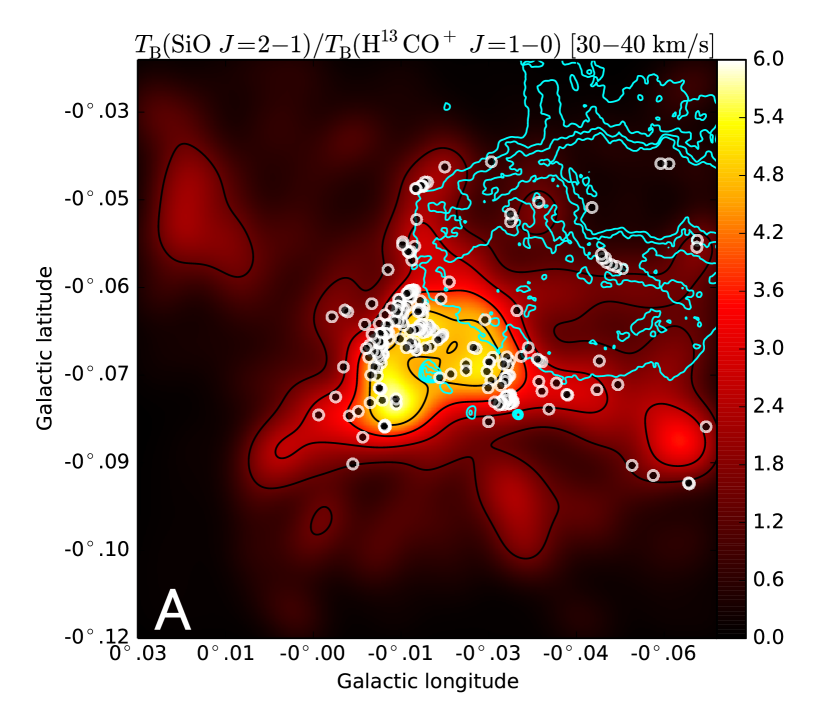
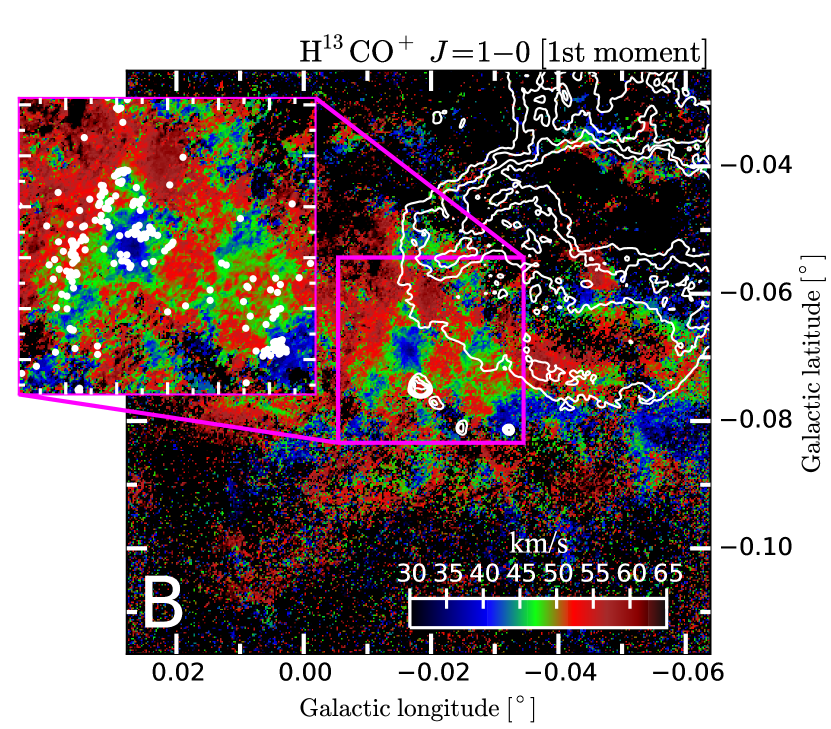
Figure 15: [A] Color map with contours (black solid line) of $R_{T}=T_{\rm B}({\rm SiO}~{}J=2-1)/T_{\rm B}({\rm H^{13}CO^{+}}~{}J=1-0)$ smoothed to $26^{\prime\prime}$ resolution. The ratio scale is shown in the color bar on the right-hand side of the panel, and the contour levels are 1.4,2.5,3.6,4.7 and 5.8. The black filled circles show the positions of the 44GHz methanol masers. The 6cm continuum emission is shown by the cyan contours, and the contour levels are $\rm 0.01,0.02,0.03$ and $0.04\rm~{}Jy/beam$. The 6cm continuum emission indicates the compact HII regions A-D and the Sgr A east. [B] First moment map in the ${\rm H^{13}CO^{+}}~{}J=1-0$ emission line with the 6cm continuum emission indicated by white contours. The inset map of panel B shows the first moment map with the positions of the 44GHz methanol masers (white filled circles). We supply the RGB movie (http://www.vsop.isas.jaxa.jp/~nakahara/figure_uehara/201812/map_h13co+_6km_rgb.mp4)

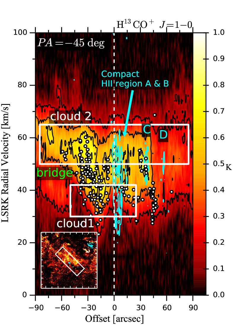
Figure 16: Psition-velocity diagram along four HII regions with a position angle of $-45^{\circ}$ in the ${\rm H^{13}CO^{+}}$ emission line with black contours. The vertical white dashed lines show offset $=0\rm~{}arcsec$. The cyan contours show the $\rm H_{42}\alpha$ recombination line of our ALMA data. Open black circles indicate the positions of the 44 GHz class I methanol maser. The inset map shows the $T_{\rm peak}$ maps of the ${\rm H^{13}CO^{+}}~{}J=1-0$ emission line. The white open rectangles on the inset maps indicate the cutting direction of each position-velocity diagram with the cutting widths of $1\rm~{}arcmin$. The velocity resolution is $2\rm~{}km~{}s^{-1}$.

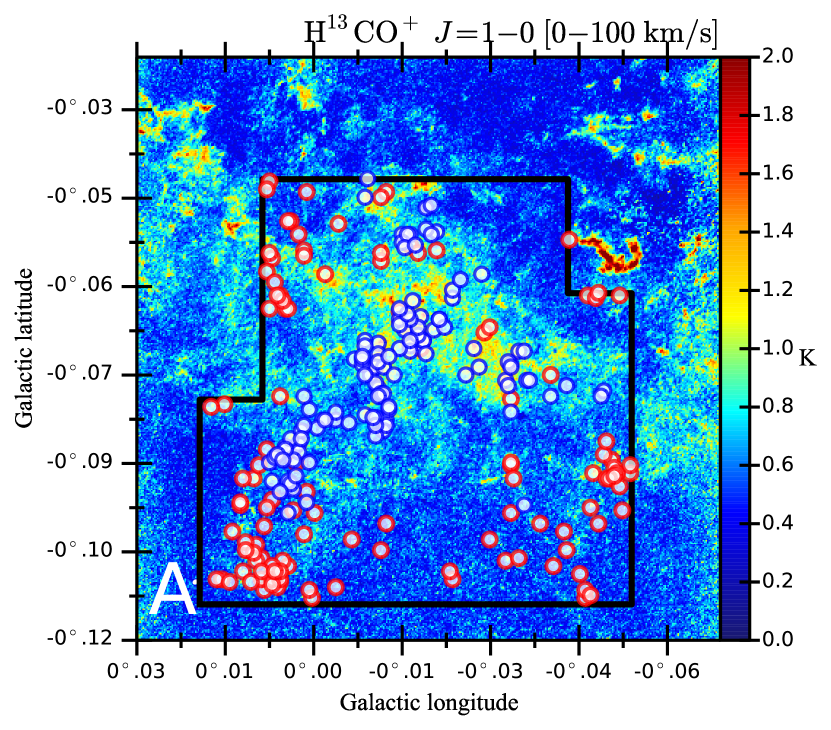
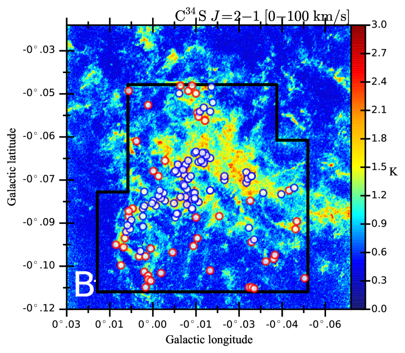
Figure 17: [A] Positions of the identified bound cores with $\alpha<2$ on the $T_{\rm peak}$ map of the ${\rm H^{13}CO^{+}}~{}J=1-0$ emission line in the velocity range of $V_{\rm LSR}=0-100\rm~{}km~{}s^{-1}$. The intensity scale is in brightness temperature units of K and is shown in the color bar on the right-hand side of the panel. The blue circles indicate the bound cores in the CCC region and the red circles indicate the bound cores in the non-CCC region. The cores outside the polygon by the black thick line are rejected. [B] Positions of the identified bound cores on the $T_{\rm peak}$ map of the ${\rm C^{34}S}$ emission line in the velocity range of $V_{\rm LSR}=0-100\rm~{}km~{}s^{-1}$.

5.4.2 The comparison of the densities of the bound cores between the CCC and Non-CCC regions

We analyze the bound cores statistically in order to estimate the influence of the CCC. A total of 119 bound ${\rm H^{13}CO^{+}}$ cores are located in the CCC region, while 122 bound cores are located in the non-CCC region (see Figure 17-A). The percentage of the bound cores in the CCC is $49\%(=119/241)$, while that in the non-CCC region $51\%~{}(=122/241)$. The physical parameters of the bound ${\rm H^{13}CO^{+}}$ cores in the CCC and non-CCC regions are summarized in Table 6. Additionally, the pixel number ratio of the CCC region to the non-CCC region is $14\%~{}(=\rm 5329920~{}pixels/37077957~{}pixels)$ in the core identified region. Thus, the area of the CCC region is much smaller than that of the non-CCC region, but the numbers of the bound cores in the CCC and non-CCC regions are similar to each other. The surface density of the cores in the CCC region is an order of magnitude larger than that in the non-CCC region. On the other hand, the physical parameters of the bound ${\rm C^{34}S}$ cores in the CCC and non-CCC regions are summarized in Table 7. The positions of these cores are shown in Figure 17-B. The number ratio of the bound ${\rm C^{34}S}$ cores in the CCC region to all the cores is $64\%~{}(=82/129)$, while that in the non-CCC region $37\%~{}(=48/129)$.

Figure 18-A shows the CDFs for the number densities of the bound ${\rm H^{13}CO^{+}}$ cores in the CCC (black line) and non-CCC (red line) regions. The average and range of the number densities are indicated in Figure 18-A. The distribution of the core number densities in the CCC region seems to be biased to a larger density than that in the non-CCC region. Similarly, the distribution of the column densities toward the bound cores in the CCC region is biased to a larger column density than that in the non-CCC region in Figure 19-A. Especially, there exit 26 cores with more than $8.1\times 10^{23}\rm~{}cm^{-2}$ only in the CCC region.

The bound ${\rm C^{34}S}$ cores in the CCC region also have larger number and column densities than those in the non-CCC region as shown in Figure 18-B and 19-B. There are 27 cores with more than $5.6\times 10^{23}\rm~{}cm^{-2}$ only in the CCC region. Consequently, it is most likely that the CCC compresses the molecular gas and increases the number of the bound cores with high densities.

5.4.3 The comparison of the masses of the bound cores in the CCC and non-CCC regions

Figure 20-A shows the histograms of the LTE masses of the bound ${\rm H^{13}CO^{+}}$ cores in the CCC (blue bar) and non-CCC (red bar) regions. The average and range of the masses of the bound ${\rm H^{13}CO^{+}}$ cores in the CCC region are $1300\pm 970~{}M_{\odot}$ and $190-4500~{}M_{\odot}$, respectively. Meanwhile, the average and range of the masses in the non-CCC region are $610\pm 510~{}M_{\odot}$ and $48-2400~{}M_{\odot}$, respectively. The mean mass of the bound ${\rm H^{13}CO^{+}}$ cores in the CCC region seems larger than that in the non-CCC regions.

The mass distribution peak of the cores in the CCC region is at $\log_{10}\left(M_{\rm LTE}~{}[M_{\odot}]\right)=3$ derived by the Gaussian fitting, whereas that in the non-CCC region is at $\log_{10}\left(M_{\rm LTE}~{}[M_{\odot}]\right)=2.7$. Note that the massive bound cores with masses of $2400~{}M_{\odot}$ or more exist only in the CCC region as well as the dense cores with more than $8.1\times 10^{23}\rm~{}cm^{-2}$ exist only in the CCC region. The total bound core mass in the CCC region is $68~{}\%(=1.6\times 10^{5}~{}M_{\sun}/2.3\times 10^{5}~{}M_{\sun})$ of the total bound core mass in the whole 50MC. It is likely that the CCC efficiently formed the massive bound ${\rm H^{13}CO^{+}}$ cores by compressing the molecular gas.

Additionally, the total mass of the bound ${\rm C^{34}S}$ core in the CCC region is $76\%(=1.3\times 10^{5}M_{\odot}/1.7\times 10^{5}M_{\odot})$ of the total bound core mass in the whole 50MC. The mass distribution peak of the cores in the CCC region is at $\log_{10}\left(M_{\rm LTE}~{}[M_{\odot}]\right)=3.1$ derived by the Gaussian fitting, whereas that in the non-CCC region is at $\log_{10}\left(M_{\rm LTE}~{}[M_{\odot}]\right)=2.8$ in Figure 20-B. Note that the massive bound cores with masses of $3000~{}M_{\odot}$ or more exist only in the CCC region as well as the bound cores with high column densities exist only in the CCC region. It is also likely that the CCC efficiently formed the massive bound ${\rm C^{34}S}$ cores by compressing the molecular gas.

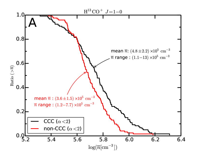
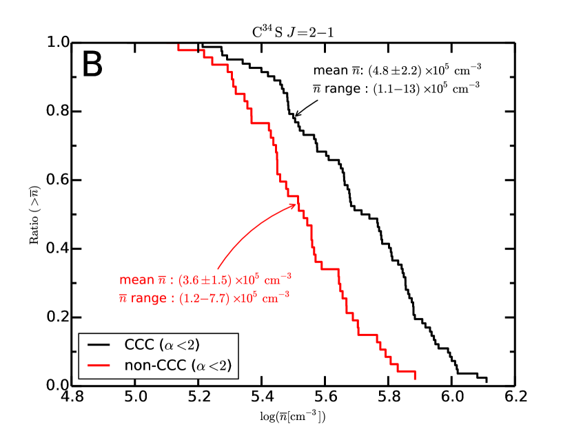
Figure 18: [A] CDF of the bound ${\rm H^{13}CO^{+}}~{}J=1-0$ core number density. The black thick line shows the distribution of the bound cores in the CCC region, while the red thick line shows the distribution of the bound cores in the non-CCC region. [B] CDF of the ${\rm C^{34}S}~{}J=2-1$ core number density.

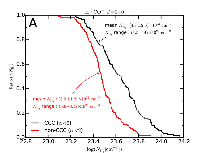
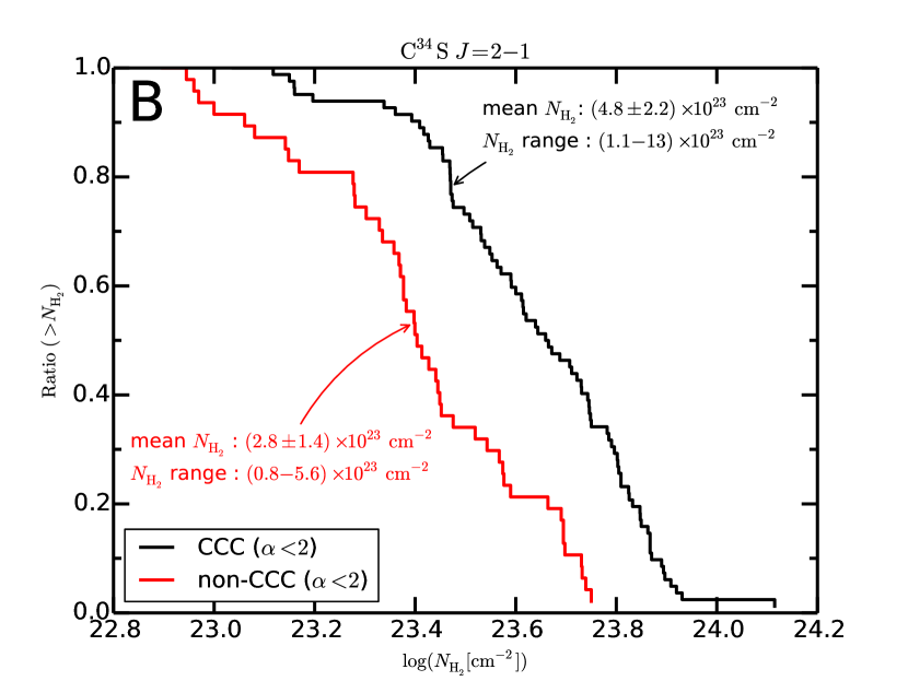
Figure 19: [A] CDF of the bound ${\rm H^{13}CO^{+}}~{}J=1-0$ core column density. The black thick line shows the distribution of the bound cores in the CCC region, while the red thick line shows the distribution of the bound cores in the non-CCC region. [B] CDF of the ${\rm C^{34}S}~{}J=2-1$ core column density.

Figure 21-A shows the CDFs for the LTE masses of the bound ${\rm H^{13}CO^{+}}$ cores in the CCC (black line) and non-CCC (red line) regions. The distribution of the core LTE masses in the CCC region is biased to a larger mass than that in the non-CCC region. The CMFs of the bound ${\rm H^{13}CO^{+}}$ cores within the CCC and non-CCC regions in the 50MC are shown by the blue circles and the red diamonds in the Figure 22-A, respectively. We apply single power-law functions of Eq. (11) to the CMFs in the CCC and non-CCC regions in the mass range of $>600~{}M_{\odot}$ and $>200~{}M_{\odot}$, respectively. The best-fit values of $\alpha_{\rm cmf}$ in the CCC and non-CCC regions are $1.38\pm 0.20$ and $1.37\pm 0.13$, respectively. The CMFs in the CCC and non-CCC regions show top-heavy distributions compared with that in the Orion A (Ikeda et al., 2007) and in the previous work (Tsuboi et al., 2015), and the CMF index in the CCC region is consistent with that in the non-CCC region within the uncertainties. We conclude that the slope of the CMF was not changed so much, but the compression by the CCC efficiently formed the massive bound ${\rm H^{13}CO^{+}}$ cores, especially the bound cores with masses of $2400~{}M_{\odot}$ or more.

On the other hand, the CMF index of the bound ${\rm C^{34}S}$ cores in the CCC region is consistent with that in the non-CCC region within the uncertainties (see Figure 22). Figure 21-B shows the CDFs for the LTE masses of the bound ${\rm C^{34}S}$ cores in the CCC (black line) and non-CCC (red line) regions. The distribution of the core LTE masses in the CCC region is biased to a larger mass than that in the non-CCC region. The analysis of the bound ${\rm C^{34}S}$ cores gives the same conclusion as in the analysis of the bound ${\rm H^{13}CO^{+}}$ cores; the slope of the CMF is not changed so much in the mass range of $100~{}M_{\odot}$ to $3000~{}M_{\odot}$ but the CCC efficiently formed the massive bound cores.

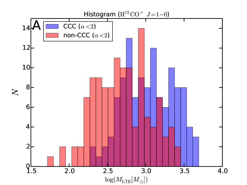
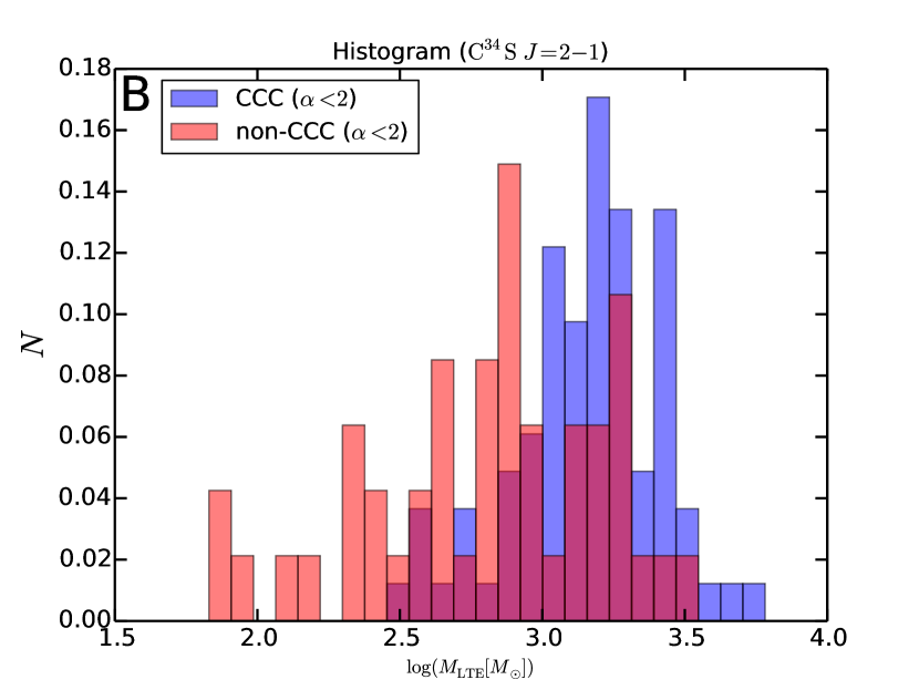
Figure 20: (A) Histogram of the masses of the bound ${\rm H^{13}CO^{+}}$ cores in the CCC region (blue bars) and that in the non-CCC region (red bars). (B) Histogram of the masses of the bound ${\rm C^{34}S}$ cores in the CCC region (blue bars) and that in the non-CCC region (red bars).

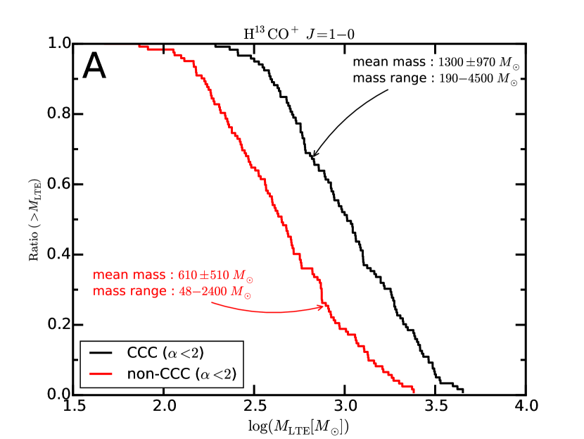
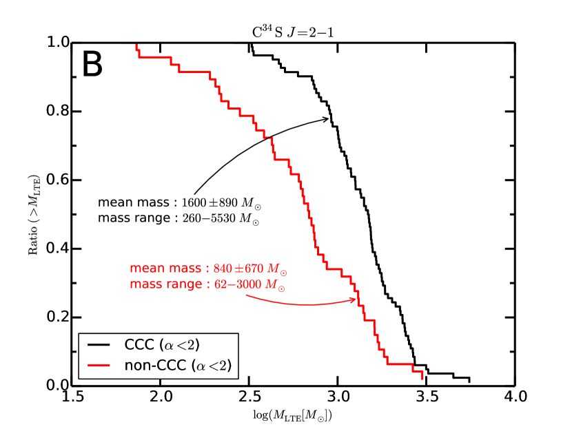
Figure 21: [A] CDF of the bound ${\rm H^{13}CO^{+}}~{}J=1-0$ core LTE mass. The black thick line shows the distribution of the bound cores in the CCC region, while the red thick line shows the distribution of the bound cores in the non-CCC region. [B] CDF of the ${\rm C^{34}S}~{}J=2-1$ core LTE mass.

Additionally, the 50MC interacts with the Sgr A east (Ho et al., 1985) (e.g. Figure 1-C in this paper). We discuss the effect of the interaction with the Sgr A east on the bound cores because it is possible that the 50MC has been compressed by the Sgr A east. A region of $l<-0\fdg 016$ which is the right half region of the core identified region, is defined as the interaction region with the Sgr A east, whereas a region of $l>-0\fdg 016$ is defined as the non-interaction region. Among the bound ${\rm H^{13}CO^{+}}$ cores, 83 cores are located in the interaction region, while 158 cores are located in the non-interaction region. The average and range of the LTE masses are shown in Figure 23-A and the average and range in the interaction region are similar to those in the non-interaction region. The distributions are also consistent with each other. Additionally, we applied the same analysis to the cores only in the CCC region and obtained the same results. The bound core formation might be affected by the Sgr A east, but it is likely that the influence of the Sgr A east on the bound core distribution is small, suggesting that the compression of the 50MC by the Sgr A east does not have a significant influence on the bound core formation.

We conclude that the molecular gas compression by the CCC efficiently formed the massive bound cores, especially the bound cores with high masses of $\sim 2500-3000~{}M_{\odot}$ or more, even if the slope of the CMF is not changed so much by the CCC.

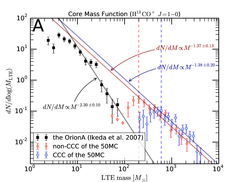
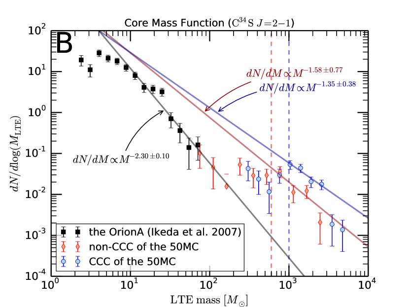
Figure 22: (A) Core mass function of the bound ${\rm H^{13}CO^{+}}$ cores in the CCC region (blue circles) with the best-fitted single power-law line (blue solid line). The power-law index is $1.38\pm 0.20$. The vertical blue dashed line shows $M_{\rm LTE}=600M_{\odot}$ and we analyze the CMF in the range of $>600M_{\odot}$. The core mass function in the non-CCC region is shown by the red diamonds with the best-fitted single power-law line (red dashed line). The power-law index is $1.37\pm 0.13$. The vertical red dashed line shows $M_{\rm LTE}=200M_{\odot}$ and we analyze the CMF in the range of $>200M_{\odot}$. The core mass function of the Orion A cloud is shown by the black squares (Ikeda et al., 2007). (B) Core mass function of the bound ${\rm C^{34}S}$ cores in the CCC region (blue circles) with the best-fitted single power-law line (blue solid line). The power-law index is $1.35\pm 0.38$. The vertical blue dashed line shows $M_{\rm LTE}=1000M_{\odot}$ and we analyze the CMF in the range of $>1000M_{\odot}$. The core mass function in the non-CCC region is shown by the red diamonds with the best-fitted single power-law line (red dashed line). The power-law index is $1.58\pm 0.77$. The vertical red dashed line shows $M_{\rm LTE}=600M_{\odot}$ and we analyze the CMF in the range of $>600M_{\odot}$.

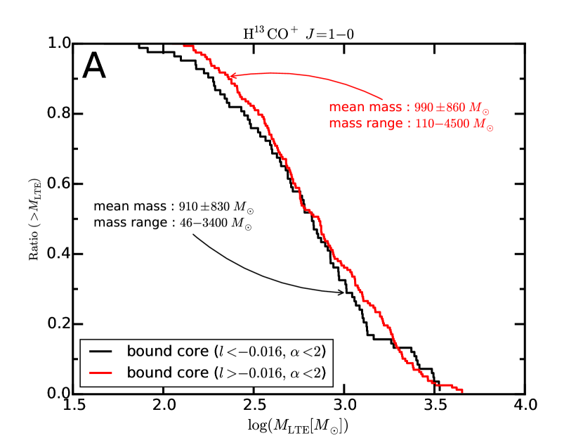
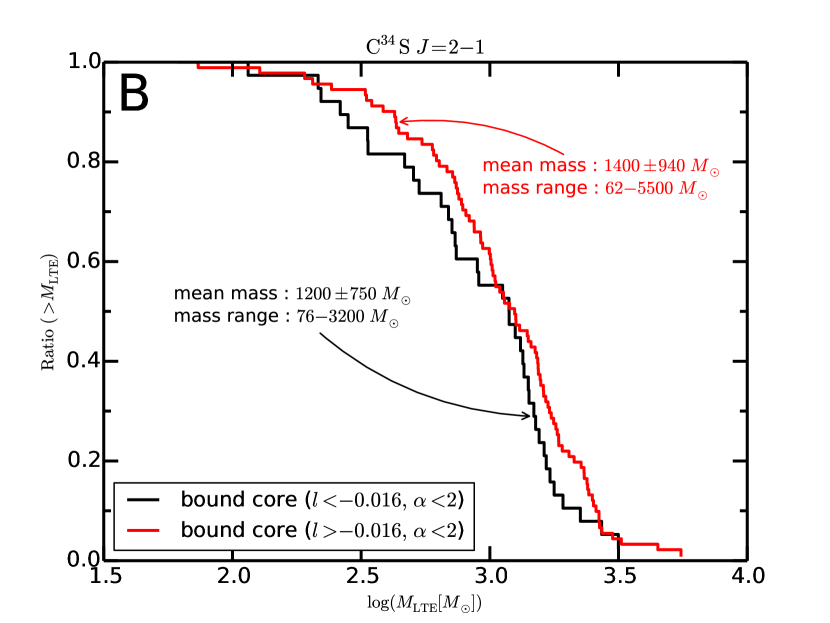
Figure 23: [A] CDF of the LTE mass of the bound ${\rm H^{13}CO^{+}}~{}J=1-0$ core. The black thick line shows the distribution in the interaction region of $l<-0\fdg 016$, while the red thick line shows the distribution in the interaction region of $l>-0\fdg 016$. [B] CDF of the LTE mass of the bound ${\rm C^{34}S}~{}J=2-1$ core.

Table 2: The best-fit parameters of a single power-law for the CMFs.

Parameter	The whole of the 50MC	CCC	Non-CCC
$({\rm H^{13}CO^{+}}~{}J=1-0)$
$\alpha_{\rm cmf}$	$1.48\pm 0.14$	$1.38\pm 0.20$	$1.37\pm 0.13$
$\chi^{2}/{\rm dof}$	$0.66~{}(4.63/7)$	$1.11~{}(9.95/9)$	$0.83~{}(6.67/8)$
Parameter	The whole of the 50MC	CCC	Non-CCC
$({\rm C^{34}S}~{}J=2-1)$
$\alpha_{\rm cmf}$	$1.15\pm 0.24$	$1.35\pm 0.38$	$1.58\pm 0.77$
$\chi^{2}/{\rm dof}$	$1.46~{}(4.36/3)$	$0.53~{}(1.07/2)$	$1.96~{}(1.96/1)$

Finally, Figure 24 shows the smallest $\alpha$ core (ID 1706) and the most massive core (ID 1530) in the bound ${\rm H^{13}CO^{+}}$ cores. These bound cores are located on a line where the $\rm H_{II}$ regions A to C line up and at the region considered as the shock front discussed in §5.4.1. The radial velocities of the HII regions are $40-48\rm~{}km~{}s^{-1}$ as shown in Figure 16 and the smallest alpha core and the most massive core have the radial velocities of $40$ and $38\rm~{}km~{}s^{-1}$, respectively. Additionally, in §5.4.1, we argued that the clouds with $V_{\rm LSR}\sim 35$ and $\sim 55\rm~{}km~{}s^{-1}$ collide and that the shock front propagates southwest to northeast. It is likely that the HII regions A-C in the southwest part of the line formed first in the CCC process. This is because the HII regions A-C have ages of $\sim 10^{4-5}$ years (Yusef-Zadeh et al., 2010; Mills et al., 2011), which are smaller shorter than the dynamical time scale of the CCC. The dynamical time scale of the CCC is $L/V_{\rm CCC}\sim 5\times 10^{5}$ years, assuming that the size of the 50MC, $L$, is $\sim 10\rm~{}pc$ and the collision velocity, $V_{\rm CCC}$, is $55~{}{\rm km~{}s^{-1}}-35~{}{\rm km~{}s^{-1}}=20~{}{\rm km~{}s^{-1}}$. Considering the lining up of the bound cores and the compact $\rm HII$ regions of A, B, and C and that the ages of the HII regions are smaller than the CCC time scale, the star formation might have occurred sequentially from the compact $\rm HII$ region C to A owing to the CCC, and the bound cores would produce massive stars to evolve into new compact $\rm HII$ regions.

We will discuss the possibility of the massive star formation in the bound cores in the 50MC in a future paper.

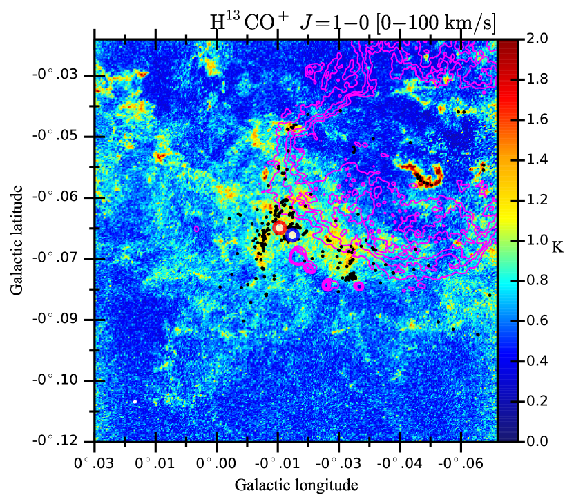
Figure 24: The bound ${\rm H^{13}CO^{+}}$ core with smallest $\alpha$ of 0.4 is plotted on the $T_{\rm peak}$ map of the ${\rm H^{13}CO^{+}}~{}J=1-0$ emission line in the velocity range of $V_{\rm LSR}=0-100\rm~{}km~{}s^{-1}$ with the blue open circle. The red open circle shows the most massive bound ${\rm H^{13}CO^{+}}$ core of $4500~{}M_{\odot}$. The 6cm continuum emission is shown by the magenta contours. The positions of the 44 GHz methanol masers are shown by the black filled circles.

6 Summary

We observed the whole of the 50MC by ALMA in the H¹³CO${}^{+}~{}J=1-0$ and ${\rm C^{34}S}~{}J=2-1$ emission lines with the high sensitivity of $\sigma=0.16\rm~{}K$ and with the high angular resolution of $2\farcs 04\times 1\farcs 41$ and $2\farcs 00\times 1\farcs 35$, respectively. Our results and conclusions are summarized as follows:

• We identified 3293 and 3192 molecular cloud core candidates in the ${\rm H^{13}CO^{+}}~{}J=1-0$ and ${\rm C^{34}S}~{}J=2-1$ maps, respectively, and the number of the identified cores in these data is 100 times larger than that in the previous work in the CS $J=1-0$ emission line maps and is enough for good statistics. The mean mass of the identified dense cores is $\sim 15$ times larger than that in the Orion A cloud, although the radii of the core candidates in the 50MC are similar to those in the Orion A.

• The bound ${\rm H^{13}CO^{+}}$ cores with a virial parameter of less than 2 are $7\%~{}(=241/3293)$ of all the identified ${\rm H^{13}CO^{+}}$ core candidates. The bound ${\rm C^{34}S}$ cores are $\sim 4\%~{}(=129/3192)$ of all the identified ${\rm C^{34}S}$ core candidates.

• The mean masses of the ${\rm H^{13}CO^{+}}$ and ${\rm C^{34}S}$ bound cores are $960\pm 850M_{\odot}$ and $1300\pm 890~{}M_{\odot}$, respectively. The mass ratio of the total bound ${\rm H^{13}CO^{+}}$ core mass to the total gas mass is $18~{}\%(=2.3\times 10^{5}~{}M_{\sun}/1.3\times 10^{6}~{}M_{\sun})$. On the other hand, the mass ratio of the total bound ${\rm C^{34}S}$ core mass is $23~{}\%(=1.7\times 10^{5}~{}M_{\sun}/7.3\times 10^{5}~{}M_{\sun})$. These low mass ratios are consistent with the low star formation efficiency in the CMZ.

• The velocity widths of the cores in the 50MC are 10 times larger than those of the cores in the Orion A cloud, but the slopes of the $R$-$\Delta V$ relations in the CCC and non-CCC regions of the 50MC are agree with those in the Orion A. The bound cores in the 50MC and the Orion A cloud have similar radii, but the LTE masses and the virial parameters in the 50MC are one to two orders of magnitude larger than those in the Orion A. The virial parameters in the 50MC are $\sim 10-100$ times larger than those in the Orion A. Most of the core candidates are not bound by self-gravity because of the large virial parameters. The CMFs of the bound cores in the 50MC have top-heavy distributions (${\rm H^{13}CO^{+}}:1.48\pm 0.14$; ${\rm C^{34}S}:1.15\pm 0.24$) to that of the Orion A cloud in the high-mass parts.

• The number ratio of the bound ${\rm H^{13}CO^{+}}$ cores to all the bound cores in the CCC region ($49\%=119/241$) is as large as that in the non-CCC region ($51\%=122/241$). The distribution of the core number and column densities in the CCC region seems to be biased to a larger density than those in the non-CCC region. Especially, 26 cores with more than $8.1\times 10^{23}\rm~{}cm^{-2}$ exist only in the CCC region. The bound ${\rm C^{34}S}$ cores also have a density distribution biased toward the dense side. These results indicate that the CCC compresses the molecular gas and increases the number of the bound cores with high densities.

• The mean mass in the CCC region ($1300\pm 970~{}M_{\odot}$) is also $\sim 2$ times larger than that in the non-CCC region ($610\pm 510~{}M_{\odot}$). The total bound core mass ratio in the CCC region to the all regions is $68~{}\%(=1.6\times 10^{5}~{}M_{\sun}/2.3\times 10^{5}~{}M_{\sun})$. The mass distribution peak of the cores in the CCC region is also positioned on the larger mass side than that in the non-CCC region. In addition, the massive bound cores with masses of $2400~{}M_{\odot}$ or more exist only in the CCC region. Additionally, the area of the CCC region is much smaller than that of the non-CCC region, but the numbers of the bound cores in the CCC and non-CCC regions are similar to each other. However, the slopes of the CMFs for the bound ${\rm H^{13}CO^{+}}$ cores in the CCC and non-CCC regions are $1.38\pm 0.20$ and $1.37\pm 0.13$ in the mass range of $>600~{}M_{\odot}$, respectively. Thus, the slope of the CMF is not changed so much in the mass range of $>600~{}M_{\odot}$, but the compression by the CCC efficiently formed the massive bound ${\rm H^{13}CO^{+}}$ cores.

• The number ratio of the bound ${\rm C^{34}S}$ cores to all the cores in the CCC region ($64\%=82/129$) is larger than that in the non-CCC region ($37\%=48/129$). The mean mass in the CCC region ($1600\pm 890~{}M_{\odot}$) is also $\sim 2$ times larger than that in the non-CCC region ($840\pm 670~{}M_{\odot}$). The total bound core mass ratio in the CCC region to the all regions is $76\%(=1.3\times 10^{5}M_{\odot}/1.7\times 10^{5}M_{\odot})$. The mass distribution peak of the cores in the CCC region is positioned on the larger mass side than that in the non-CCC region. Additionally, the massive bound cores with masses of $3000~{}M_{\odot}$ or more exist only in the CCC region. The slopes of the CMFs for the bound ${\rm H^{13}CO^{+}}$ cores in the CCC and non-CCC regions are $1.35\pm 0.38$ and $1.58\pm 0.77$ in the mass range of $1000~{}M_{\odot}$ to $3000~{}M_{\odot}$, respectively.

We conclude that the compression by the CCC efficiently formed the massive bound cores, especially the bound cores in high-mass end of $\sim 2500-3000$ or more, even if the CMF slope is not changed so much by the CCC.

Table 3: The property of identified molecular cloud core candidates in the ${\rm H^{13}CO^{+}}~{}J=1-0$ emission line. The columns from 2 to 4 are the three-dimensional positions of the most intense pixels in the core candidates with $T_{\rm B.peak}$ in the column 7 and those from 5 to 12 are the estimated parameters. The last column indicates whether each core candidate is located in the CCC region or not. In the end of the tables, we summarize the mean, standard deviation, maximum and minimum values of each parameter.

No.	$l$	$b$	$V_{\rm LSR}$	$R$	$\Delta V$	$T_{\rm B,peak}$	$\frac{M_{\rm vir}}{10^{2}}$	$\frac{M_{\rm LTE}}{10^{2}}$	$\alpha$	$\frac{\overline{n}}{10^{5}}$	$\frac{p_{\rm ex}/k_{\rm B}}{10^{8}}$	CCC/
	[deg]	[deg]	[km/s]	[pc]	[km/s]	[K]	$[M_{\odot}]$	$[M_{\odot}]$		$[\rm cm^{-3}]$	$[\rm K~{}cm^{-3}]$	non-CCC
1	0.0175	-0.1042	56	0.156	6.5	0.69	14	3.2	4.4	2.9	5.9	non-CCC
2	0.0175	-0.0938	42	0.311	11	0.75	82	1.3	62	0.15	1.2	non-CCC
3	0.0175	-0.0892	58	0.285	12	0.74	79	2.4	33	0.36	2.8	non-CCC
4	0.0171	-0.1047	68	0.120	7.4	0.65	14	0.12	120	0.24	0.78	non-CCC
5	0.0171	-0.1001	14	0.141	5.7	0.55	9.7	0.17	56	0.21	0.42	non-CCC
6	0.0171	-0.0826	58	0.163	6.9	0.78	16	1.8	8.7	1.5	3.8	non-CCC
7	0.0171	-0.0805	62	0.160	8.5	0.68	24	0.79	31	0.67	2.9	non-CCC
8	0.0171	-0.0805	46	0.212	7.5	0.67	25	0.71	36	0.26	0.87	non-CCC
9	0.0171	-0.0797	54	0.143	5.3	0.68	8.4	3.4	2.5	4.0	4.0	non-CCC
10	0.0171	-0.0793	64	0.163	10	0.78	35	0.60	59	0.48	3.0	non-CCC
11	0.0167	-0.1088	68	0.120	6.6	0.64	11	2.6	4.2	5.2	11	non-CCC
12	0.0167	-0.1072	54	0.069	5.0	0.66	3.6	0.87	4.1	9.1	10	non-CCC
13	0.0167	-0.1063	46	0.110	2.6	0.68	1.5	0.098	16	0.26	0.097	non-CCC
14	0.0167	-0.1026	94	0.144	7.0	0.56	15	2.2	6.7	2.5	6.4	non-CCC
15	0.0167	-0.0876	68	0.155	7.2	0.73	17	0.49	35	0.45	1.4	non-CCC
16	0.0167	-0.0867	68	0.170	7.3	0.70	19	1.2	15	0.87	2.7	non-CCC
17	0.0167	-0.0818	54	0.160	6.7	0.67	15	5.0	3.0	4.2	7.8	non-CCC
18	0.0163	-0.1105	30	0.147	7.3	0.73	17	3.0	5.6	3.2	8.7	non-CCC
19	0.0163	-0.1076	66	0.092	8.4	0.69	14	0.48	28	2.2	9.0	non-CCC
20	0.0163	-0.1063	34	0.098	6.9	0.68	9.7	1.6	6.2	5.8	14	non-CCC
21	0.0163	-0.1055	40	0.174	12	0.72	54	0.53	100	0.35	3.1	non-CCC
22	0.0163	-0.1042	26	0.084	9.1	0.73	14	1.2	12	7.1	33	non-CCC
23	0.0163	-0.1042	46	0.151	6.1	0.71	12	3.0	3.8	3.0	5.0	non-CCC
24	0.0163	-0.1038	68	0.091	9.2	0.77	16	0.084	190	0.39	2.0	non-CCC
25b	0.0163	-0.0801	56	0.162	7.8	0.97	21	10	2.0	8.6	16	non-CCC
26	0.0163	-0.0797	64	0.155	9.3	0.72	28	0.71	40	0.65	3.3	non-CCC
27	0.0155	-0.1092	54	0.114	5.8	0.81	8.0	1.7	4.8	4.0	6.5	non-CCC
28b	0.0155	-0.1072	64	0.119	4.4	0.76	4.8	2.7	1.8	5.4	2.9	non-CCC
29	0.0155	-0.1072	52	0.084	6.8	0.74	8.2	1.6	5.2	9.2	21	non-CCC
30	0.0155	-0.1047	64	0.104	4.2	0.67	3.9	0.14	27	0.44	0.46	non-CCC
Ave.				0.164	6.7	0.80	18	2.3	20	1.7	3.5
Std.				0.040	2.1	0.20	15	3.7	25	2.0	5.5
Max.				0.330	22	2.1	230	45	450	25	120
Min.				0.042	2.1	0.50	0.81	0.043	0.40	0.10	-11

Table 4: The property of identified molecular cloud core candidates in the ${\rm C^{34}S}~{}J=2-1$ emission line. The columns from 2 to 4 are the three-dimensional positions of the most intense pixels in the core candidates with $T_{\rm B.peak}$ in the column 7 and those from 5 to 12 are the estimated parameters. The last column indicates whether each core candidate is located in the CCC region or not. In the end of the tables, we summarize the mean, standard deviation, maximum and minimum values of each parameter.

No.	$l$	$b$	$V_{\rm LSR}$	$R$	$\Delta V$	$T_{\rm B,peak}$	$\frac{M_{\rm vir}}{10^{2}}$	$\frac{M_{\rm LTE}}{10^{2}}$	$\alpha$	$\frac{\overline{n}}{10^{5}}$	$\frac{p_{\rm ex}/k_{\rm B}}{10^{8}}$	CCC/
	[deg]	[deg]	[km/s]	[pc]	[km/s]	[K]	$[M_{\odot}]$	$[M_{\odot}]$		$[\rm cm^{-3}]$	$[\rm K~{}cm^{-3}]$	non-CCC
1	0.0175	-0.0947	56	0.171	11	0.65	40	0.16	250	0.11	0.75	non-CCC
2	0.0175	-0.0788	58	0.114	6.3	0.79	9.6	0.27	36	0.62	1.5	non-CCC
3	0.0171	-0.1063	58	0.099	4.0	0.61	3.3	0.46	7.3	1.6	1.4	non-CCC
4	0.0171	-0.1047	70	0.230	9.7	0.78	46	0.29	160	0.081	0.47	non-CCC
5	0.0171	-0.1017	72	0.135	6.3	0.70	11	0.13	87	0.18	0.44	non-CCC
6	0.0171	-0.1013	48	0.171	12	0.65	56	0.13	430	0.091	0.86	non-CCC
7	0.0171	-0.0851	66	0.197	10	0.68	44	0.46	97	0.21	1.3	non-CCC
8	0.0171	-0.0805	58	0.159	4.9	0.78	8.0	0.51	16	0.44	0.60	non-CCC
9	0.0171	-0.0805	62	0.185	7.8	0.67	24	0.27	88	0.15	0.55	non-CCC
10	0.0167	-0.1084	78	0.207	12	0.61	66	0.48	140	0.19	1.7	non-CCC
11	0.0167	-0.0917	28	0.114	5.8	0.85	7.9	0.11	71	0.26	0.53	non-CCC
12	0.0167	-0.0897	54	0.172	11	0.56	41	0.19	210	0.13	0.90	non-CCC
13	0.0167	-0.0872	30	0.191	15	0.67	92	0.19	480	0.095	1.3	non-CCC
14	0.0167	-0.0826	64	0.204	10	0.65	47	0.54	86	0.22	1.5	non-CCC
15	0.0163	-0.0951	66	0.131	7.6	0.66	16	0.075	210	0.12	0.41	non-CCC
16	0.0159	-0.1097	80	0.121	3.5	0.65	3.1	0.055	56	0.11	0.08	non-CCC
17	0.0159	-0.1059	34	0.131	8.9	0.69	22	0.76	28	1.2	5.5	non-CCC
18	0.0159	-0.0801	56	0.126	5.3	0.68	7.5	1.1	6.6	2.0	2.9	non-CCC
19	0.0155	-0.1105	32	0.143	5.3	0.69	8.6	1.1	7.9	1.3	1.9	non-CCC
20	0.0155	-0.1105	62	0.164	8.2	0.66	23	1.4	17	1.1	4.1	non-CCC
21	0.0155	-0.1080	30	0.133	6.7	0.94	13	1.4	9.3	2.0	4.9	non-CCC
22	0.0155	-0.1042	48	0.147	5.8	0.81	10	0.20	51	0.22	0.45	non-CCC
23	0.0155	-0.0930	54	0.290	12	0.65	87	0.57	150	0.081	0.70	non-CCC
24	0.0155	-0.0813	54	0.167	5.9	0.66	12	1.6	7.7	1.2	2.2	non-CCC
25	0.0155	-0.0809	58	0.134	3.6	0.77	3.7	0.32	12	0.45	0.33	non-CCC
26	0.0155	-0.0793	58	0.135	10	0.74	29	0.31	92	0.44	2.7	non-CCC
27	0.0150	-0.1038	14	0.226	13	0.60	80	2.7	30	0.80	7.9	non-CCC
28	0.0150	-0.1026	52	0.104	12	0.67	31	0.57	55	1.7	15	non-CCC
29	0.0150	-0.0934	24	0.110	4.4	0.69	4.4	0.085	52	0.22	0.25	non-CCC
30	0.0146	-0.1059	30	0.160	16	0.68	83	1.5	56	1.3	19	non-CCC
Ave.				0.171	6.8	1.0	19	1.9	39	1.0	2.4
Std.				0.042	2.0	0.40	14	3.6	52	1.4	3.5
Max.				0.319	20	3.9	140	55	800	15	53
Min.				0.050	2.0	0.50	0.76	0.024	0.80	0.056	-5.3

Table 5: The physical parameter of the bound ${\rm H^{13}CO^{+}}$ and ${\rm C^{34}S}$ cores.

${\rm H^{13}CO^{+}}$	$R$[pc]	$\Delta V[\rm km~{}s^{-1}]$	$\frac{M_{\rm vir}}{10^{2}}[M_{\odot}]$	$\frac{M_{\rm LTE}}{10^{2}}[M_{\odot}]$	$\alpha(=M_{\rm vir}/M_{\rm LTE})$	$\frac{n}{10^{5}}[\rm cm^{-3}]$
Ave.	0.170	5.4	13	9.6	1.4	5.8
Std.	0.045	1.8	11	8.5	0.37	2.7
Max.	0.302	11	75	45	2.0	21
Min.	0.067	2.1	0.81	0.48	0.40	1.9
${\rm C^{34}S}$	$R$[pc]	$\Delta V[\rm km~{}s^{-1}]$	$\frac{M_{\rm vir}}{10^{2}}[M_{\odot}]$	$\frac{M_{\rm LTE}}{10^{2}}[M_{\odot}]$	$\alpha(=M_{\rm vir}/M_{\rm LTE})$	$\frac{n}{10^{5}}[\rm cm^{-3}]$
Ave.	0.204	6.3	19	13	1.5	4.9
Std.	0.040	1.8	12	8.9	0.29	2.5
Max.	0.305	10	52	55	2.0	13
Min.	0.097	2.0	0.83	0.62	0.80	0.95

Table 6: The physical parameter of the bound ${\rm H^{13}CO^{+}}$ cores in the CCC and non-CCC regions.

CCC	$R$[pc]	$\Delta V[\rm km~{}s^{-1}]$	$\frac{M_{\rm vir}}{10^{2}}[M_{\odot}]$	$\frac{M_{\rm LTE}}{10^{2}}[M_{\odot}]$	$\alpha(=M_{\rm vir}/M_{\rm LTE})$	$\frac{n}{10^{5}}[\rm cm^{-3}]$
Ave.	0.188	6.2	18	13	1.4	6.3
Std.	0.040	1.8	13	9.7	0.36	3.2
Max.	0.302	11	75	45	2.0	21
Min.	0.100	2.8	2.6	1.9	0.40	1.9
Non-CCC	$R$[pc]	$\Delta V[\rm km~{}s^{-1}]$	$\frac{M_{\rm vir}}{10^{2}}[M_{\odot}]$	$\frac{M_{\rm LTE}}{10^{2}}[M_{\odot}]$	$\alpha(=M_{\rm vir}/M_{\rm LTE})$	$\frac{n}{10^{5}}[\rm cm^{-3}]$
Ave.	0.151	4.6	8.3	6.1	1.4	5.3
Std.	0.043	1.4	6.9	5.1	0.39	1.9
Max.	0.245	8.2	31	24	2.0	15
Min.	0.067	2.1	0.81	0.48	0.49	2.1

Table 7: The physical parameter of the bound ${\rm C^{34}S}$ cores in the CCC region.

CCC	$R$[pc]	$\Delta V[\rm km~{}s^{-1}]$	$\frac{M_{\rm vir}}{10^{2}}[M_{\odot}]$	$\frac{M_{\rm LTE}}{10^{2}}[M_{\odot}]$	$\alpha(=M_{\rm vir}/M_{\rm LTE})$	$\frac{n}{10^{5}}[\rm cm^{-3}]$
Ave.	0.212	6.8	22	16	1.5	5.6
Std.	0.033	1.6	11	8.9	0.31	2.6
Max.	0.296	10	52	55	2.0	13
Min.	0.146	3.0	3.4	2.6	0.80	0.95
Non-CCC	$R$[pc]	$\Delta V[\rm km~{}s^{-1}]$	$\frac{M_{\rm vir}}{10^{2}}[M_{\odot}]$	$\frac{M_{\rm LTE}}{10^{2}}[M_{\odot}]$	$\alpha(=M_{\rm vir}/M_{\rm LTE})$	$\frac{n}{10^{5}}[\rm cm^{-3}]$
Ave.	0.189	5.3	14	8.4	1.6	3.6
Std.	0.047	1.8	11	6.7	0.23	1.5
Max.	0.305	9.7	52	30	2.0	7.7
Min.	0.097	2.0	0.83	0.62	1.1	1.3

References

- Amo-Baladrón et al. (2011) Amo-Baladrón, M. A., Martín-Pintado, J., & Martín, S. 2011, A&A, 526, A54
- André et al. (2010) André, P., Men’shchikov, A., Bontemps, S., et al. 2010, A&A, 518, L102
- Ao et al. (2013) Ao, Y., Henkel, C., Menten, K. M., et al. 2013, A&A, 550, A135
- Barnes et al. (2017) Barnes, A. T., Longmore, S. N., Battersby, C., et al. 2017, MNRAS, 469, 2263
- Chomiuk & Povich (2011) Chomiuk, L., & Povich, M. S. 2011, AJ, 142, 197
- Christopher et al. (2005) Christopher, M. H., Scoville, N. Z., Stolovy, S. R., & Yun, M. S. 2005, ApJ, 622, 346
- Coil & Ho (2000) Coil, A. L., & Ho, P. T. P. 2000, ApJ, 533, 245
- Ekers et al. (1983) Ekers, R. D., van Gorkom, J. H., Schwarz, U. J., & Goss, W. M. 1983, A&A, 122, 143
- Figer et al. (1999) Figer, D. F., Kim, S. S., Morris, M., et al. 1999, ApJ, 525, 750
- Frerking et al. (1982) Frerking, M. A., Langer, W. D., & Wilson, R. W. 1982, ApJ, 262, 590
- Furukawa et al. (2009) Furukawa, N., Dawson, J. R., Ohama, A., et al. 2009, ApJ, 696, L115
- Ghez et al. (2005) Ghez, A. M., Salim, S., Hornstein, S. D., et al. 2005, ApJ, 620, 744
- Ghez et al. (2003) Ghez, A. M., Duchêne, G., Matthews, K., et al. 2003, ApJ, 586, L127
- Goss et al. (1985) Goss, W. M., Schwarz, U. J., van Gorkom, J. H., & Ekers, R. D. 1985, MNRAS, 215, 69P
- Güsten (1989) Güsten, R. 1989, in IAU Symposium, Vol. 136, The Center of the Galaxy, ed. M. Morris, 89
- Habe & Ohta (1992) Habe, A., & Ohta, K. 1992, PASJ, 44, 203
- Hasegawa et al. (1994) Hasegawa, T., Sato, F., Whiteoak, J. B., & Miyawaki, R. 1994, ApJ, 429, L77
- Haworth et al. (2015) Haworth, T. J., Tasker, E. J., Fukui, Y., et al. 2015, MNRAS, 450, 10
- Ho et al. (1985) Ho, P. T. P., Jackson, J. M., Barrett, A. H., & Armstrong, J. T. 1985, ApJ, 288, 575
- Ikeda et al. (2009) Ikeda, N., Kitamura, Y., & Sunada, K. 2009, ApJ, 691, 1560
- Ikeda et al. (2007) Ikeda, N., Sunada, K., & Kitamura, Y. 2007, ApJ, 665, 1194
- Inoue & Fukui (2013) Inoue, T., & Fukui, Y. 2013, ApJ, 774, L31
- McEwen et al. (2016) McEwen, B. C., Sjouwerman, L. O., & Pihlström, Y. M. 2016, ApJ, 832, 129
- McMullin et al. (2007) McMullin, J. P., Waters, B., Schiebel, D., Young, W., & Golap, K. 2007, in Astronomical Society of the Pacific Conference Series, Vol. 376, Astronomical Data Analysis Software and Systems XVI, ed. R. A. Shaw, F. Hill, & D. J. Bell, 127
- Mills et al. (2011) Mills, E., Morris, M. R., Lang, C. C., et al. 2011, ApJ, 735, 84
- Mills & Morris (2013) Mills, E. A. C., & Morris, M. R. 2013, ApJ, 772, 105
- Morris & Serabyn (1996) Morris, M., & Serabyn, E. 1996, ARA&A, 34, 645
- Ohama et al. (2010) Ohama, A., Dawson, J. R., Furukawa, N., et al. 2010, ApJ, 709, 975
- Park et al. (2004) Park, S., Muno, M. P., Baganoff, F. K., et al. 2004, ApJ, 603, 548
- Pihlström et al. (2011) Pihlström, Y. M., Sjouwerman, L. O., & Fish, V. L. 2011, ApJ, 739, L21
- Pilbratt et al. (2010) Pilbratt, G. L., Riedinger, J. R., Passvogel, T., et al. 2010, A&A, 518, L1
- Rathborne et al. (2015) Rathborne, J. M., Longmore, S. N., Jackson, J. M., et al. 2015, ApJ, 802, 125
- Savage et al. (2002) Savage, C., Apponi, A. J., Ziurys, L. M., & Wyckoff, S. 2002, ApJ, 578, 211
- Tsuboi et al. (1999) Tsuboi, M., Handa, T., & Ukita, N. 1999, ApJS, 120, 1
- Tsuboi et al. (2016) Tsuboi, M., Kitamura, Y., Miyoshi, M., et al. 2016, PASJ, 68, L7
- Tsuboi & Miyazaki (2012) Tsuboi, M., & Miyazaki, A. 2012, PASJ, 64, 111
- Tsuboi et al. (2009) Tsuboi, M., Miyazaki, A., & Okumura, S. K. 2009, PASJ, 61, 29
- Tsuboi et al. (2015) Tsuboi, M., Miyazaki, A., & Uehara, K. 2015, PASJ, 67, 109
- Tsuboi et al. (2011) Tsuboi, M., Tadaki, K.-I., Miyazaki, A., & Handa, T. 2011, PASJ, 63, 763
- Uehara et al. (2017) Uehara, K., Tsuboi, M., Kitamura, Y., Miyawaki, R., & Miyazaki, A. 2017, in IAU Symposium, Vol. 322, The Multi-Messenger Astrophysics of the Galactic Centre, ed. R. M. Crocker, S. N. Longmore, & G. V. Bicknell, 162–163
- Ungerechts et al. (1997) Ungerechts, H., Bergin, E. A., Goldsmith, P. F., et al. 1997, ApJ, 482, 245
- van der Tak et al. (2007) van der Tak, F. F. S., Black, J. H., Schöier, F. L., Jansen, D. J., & van Dishoeck, E. F. 2007, A&A, 468, 627
- Williams et al. (1994) Williams, J. P., de Geus, E. J., & Blitz, L. 1994, ApJ, 428, 693
- Yusef-Zadeh et al. (2010) Yusef-Zadeh, F., Lacy, J. H., Wardle, M., et al. 2010, ApJ, 725, 1429
- Yusef-Zadeh & Morris (1987) Yusef-Zadeh, F., & Morris, M. 1987, ApJ, 320, 545
- Yusef-Zadeh et al. (2009) Yusef-Zadeh, F., Hewitt, J. W., Arendt, R. G., et al. 2009, ApJ, 702, 178