Scaling Features of Price-Volume Cross Correlation

Abstract

Price without transaction makes no sense. Trading volume authenticates its corresponding price, so there exists mutual information and correlation between price and trading volume. We are curious about fractal features of this correlation and need to know how structures in different scales translate information. To explore the influence of investment size (trading volume), price-wise (gain/loss), and time-scale effects, we analyzed the price and trading volume and their coupling by applying the MF-DXA method. Our results imply that price, trading volume and price-volume coupling exhibit a power law and are also multifractal. Meanwhile, considering developed markets, the price-volume couplings are significantly negatively correlated. However, in emerging markets, price has less of a contribution in price-volume coupling. In emerging markets in comparison with the developed markets, trading volume and price are more independent.

1 Introduction

The beginning of a comprehensive analysis of markets requires studying the markets’ features with the consideration of some sort of scale-wise and magnitude-wise phenomena. This implies that the researcher needs to consider scaling behaviors of financial times series during the analysis. This was firstly done by Lux and Ausloos [1]. Also, some scholars investigated the multifractal features [2, 3, 4, 5, 6, 7, 8] of stock markets [1, 9, 10, 11, 12, 13], foreign exchange markets [5, 14], commodity markets [15], cryptocurrency markets [16], macro-economics time series [17], and financial multifractal network analyses [18]. Regarding to other scientific fields, some scholars have carried out fractal analysis on some phenomena in meteorology [19, 20] , text structure analysis [21], hydrogeology [22], and astronomy [23].

Among different variables in a market, the phenomenon which leads to price discovery in an auction, is translation of trading volume. In this regard, some scholars [24, 11, 25, 26, 27, 28, 29, 30, 31, 32, 33] investigated on the existence of information translation among price and trading volume. Nevertheless, high trading volume may help one to distinguish how much tendency there exists to a certain price. Hence, if a certain price corresponds to a relatively high trading volume, it can be an indication of high price reliability [25], at that time, in the market. It may lead to small spreads and also small liquidation volatilities [34] within that time-scale. To clarify the importance of investigating price-volume information together, Ausloos and Ivanova [24] combined classical technical analysis with thermodynamic proxies. Considering that from a physics point of view, it is doubtful to investigate price movements without price-volume dependencies, they obtained some fruitful measures which can model market behavior in terms of trends and amplitude of volatilities by price and trading volume time series. Since trading volume is a touchstone of how traders work in the market and translate information via their transactions, this phenomenon can shape movements in a market.

To clarify the multifractal features of price-volume coupling, Podobnik et al. [11] obtained a power-law in price-volume cross correlations. They investigated logarithmic changes of price and its corresponding volume and showed that just the cross correlation of absolute values of volatilities are statistically significant. It is noteworthy to state that in the developed markets, the entanglement of price return fluctuations and trading volume [25], leads to a situation whereby an increase in volume shall –to some extent as a turning point– increase price fluctuations. But then, a further increase in trading volume leads to lowering the price fluctuation. Meanwhile, Guo et al. [26] investigated the price-volume cross-correlation of commodities in futures markets and compared their multifractal behaviors.

In reference to the theme of this current paper, Podobnik et al. [11]; Nasiri et al. [25] and Guo et al. [26], found that price-volume cross volatilities, may have scaling behavior at the levels of time and magnitude-scales. Since it makes no sense to study price volatilities without considering the reliability which a certain price owes to trading volume, we investigate the scaling behavior of the cross correlation of price-volume volatilities. Different scaling behavior toward events of different magnitudes, causes multifractal behavior [5].

In order to reveal scaling behavior, one needs to differentiate large-scale and small-scale patterns in a stock market as complex system [6, 3, 35, 36]. Since large-scale patterns (main trends) are somehow evident they do not present much latent information [5]. Hence, initially it is necessary to apply “detrended fluctuation analysis” (DFA) for non-stationary signals. See Peng et al. [2] and also [6, 37, 38, 39, 40].

Because of psychological biases and irrational decisions of investors [41, 42, 43, 44, 45, 46]; out-of-market effects [41, 47]; uncertainty about the transparency of fundamental analysis [42, 48]; the coexistence of collective effects and noise [41, 49]; and the lagging diffusion of internal and external information between several dynamics, a situation occurs where some assumptions of the EMH (Efficient Market Hypothesis) become doubtful. In spite of the complexity aspects in financial markets such as self-organizing (in order to increase adaptability) and scaling patterns of nonlinear dynamics, we observe power-law (scale invariance) behavior in some scales [41, 50]. Industrial, economic and political cycles which are dynamic and ever changing, may cause a variability of statistical properties of time series in different scales. This is what we call ‘non-stationarity’. These behaviors cause multifractal correlations between time series. Systems which contain persistent nonlinear interactions as inputs and outputs of the constituents, may cause some simultaneous and some lagging effects to emerge. In the case of persistent information, these effects cause long-range auto-correlation (for one constituent) and long-range cross-correlation (between several constituents) [35, 38, 51, 52].

Since real-world financial time-series may be non-stationary –possess some trends– and may be limited in length, we need a method which considers limited-length effects and non-stationarity effects [23]. The mentioned methodology has been applied successfully in finance [1, 11, 53, 54, 55, 56, 57, 58, 17, 52] and has been developed to Fourier-DFA and MF-DFA [7].

Besides these references, Podobnik and Stanley [10] introduced detrended cross correlation analysis (DXA) for studying two power-law non-stationary time series. Then, Zhou [59] developed the DXA method to multifractal DXA (MF-DXA) to investigate multifractal behaviors of two power-law non-stationary time series. Moreover, to investigate coupling behavior among more than two non-stationary power-law time series, some researchers introduced Coupling-DXA method [5]. They believed that studying more than two signals in complex systems leads researchers to better understanding the FOREX market structure, and they showed that several (more than two) constituents have a scaling coupling behavior. In the case of combining the MF-DXA within magnitude-wise scales, several researchers [4, 60, 11, 61, 62] have done some efforts on detrended covariance.

Also, some scholars specifically cast light onto the detrending methods in financial markets. As a heuristic method, Caraiani and Haven [14] applied EMD (Empirical Mode Decomposition) method on the detrending process of MF-DFA. They investigated multifractality in the currencies and non-linearity of the market. In this paper, we apply multifractal detrended cross correlation analysis (MF-DXA) to investigate the scaling behavior of volatilities of price-volume coupling in markets such as the DJIA, S&P500, TOPIX, TSE and SSEC. It is shown that, the price and trading volume and their cross correlations, contain multifractal behaviors. Moreover, the correlation coefficients of their volatilities decrease with an increase of the time-scale. In section 2, a review on methodology is presented. Then in section 3, we analyze and describe the input data used in the methodology. In section 4, the empirical results are discussed and then in section 5, we provide for the conclusion.

2 Methodology

MF-DXA

The general steps of MF-DXA methodology [1, 6, 2, 37, 38, 39, 40] are as follows. Initially we convert the time series to standardized logarithmic changes. After demeaning each data-point, we execute a cumulative summation which is called profile series (Eq. 1).

$$X_{(i)} = \sum_{k=1}^{i}[x_{k}-<x>]$$

$$Y_{(i)} = \sum_{k=1}^{i}[y_{k}-<y>]$$

$$i = 1,2,....,N.$$ (1)

Where $<...>$ is the average value of the time series; $N$ is the total length; and $X_{(i)}$ and $Y_{(i)}$ are profile series. To investigate time-scale effects on series, we consider several time-scale windows with the length of $s$ which are iterated on the time series. Variable $N_{s}$ is obtained by $int(\frac{N}{4})$ which provides the maximum number of segments (with length of $s$) in each time series. Since the length $N$ may not be an integer multiple of scale length $s$, we repeat the same iteration from ending data point to starting one. It means that each non-overlapping scale window, is allocated to sequential time locations without ignoring any data points (Eq. 3). Consequently, the total number of time-wise scales would be $2N_{s}$.

In order to convert profile series to non-stationary type series, we should eliminate the main trends (large-scale behaviors) from the time series. Among lots of detrending methods (such as polynomial detrending, Fourier detrending), it is better to start from the simplest one to avoid over-fitting and also to avoid eliminating excessive amount of information. So in this study, one-degree linear detrending is applied. As follows, detrending covariance for each time-wise scale ($s$) and windows location ($\nu$) is obtained by subtracting the local trend of each window. After detrending, local deviation in each non-overlapping window is obtained.

$$N_{s}=int(\frac{N}{s})$$ (2)

$$F_{(s,\nu)}^{2} = \frac{1}{s}\sum_{j=1}^{s}|X_{(\nu-1)s+j}^{(j)}-\tilde{X}_{\nu}^{(j)}||Y_{(\nu-1)s+j}^{(j)}-\tilde{Y}_{\nu}^{(j)}|$$

$$\nu = 1,2,..,N_{s}$$

$$F_{(s,\nu)}^{2} = \frac{1}{s}\sum_{j=1}^{s}|X_{N-(\nu-N_{s})s+j}^{(j)}-\tilde{X}_{\nu}^{(j)}||Y_{N-(\nu-N_{s})s+j}^{(j)}-\tilde{Y}_{\nu}^{(j)}|$$

$$\nu = N_{s}+1,N_{s}+2,...,2N_{s};$$ (3)

where $\tilde{X}_{\nu}$ and $\tilde{Y}_{\nu}$ are local trends which are fitted polynomials in each window $\nu$ with the local length of $s$.
For small (large) scale windows, the detrended covariance will be affected by small and rapid (large and slow) fluctuations. Because of the relatively short (long) scales, on average, there will be an increase (decrease) of local effects in the detrended covariance function. Accordingly, small-scale (large-scale) behaviors are observed significantly in small (large) windows. We can further explain this by saying that monofractals are normally distributed [63] and the volatilities can be explained just by the second statistical moment, i.e. the ‘variance’. On the contrary, when it comes to multifractals, in large (small) scales, local variations are excessively large (small). As a result, to consider different behaviors of fluctuations, we magnify our concentration from small and frequent, to large and rare fluctuations by weighting them. Hence, for considering effects of events on magnitude scales, the parameter $q$ is applied. When a big $q$ is considered, a high weight is applied to the tails (rare and enormous events) of the logarithmic changes histogram.To be unbiased toward small or large variations, $q=0$ is applied.

$$F_{q}(s)=[\frac{1}{2N_{s}}\sum_{\nu=1}^{2N_{S}}{F^{2}}(s,\nu)^{q/2}]^{\frac{1}{q}}\qquad q\neq 0.$$

$$F_{q}(s)=exp{\{\frac{1}{4N_{s}}\sum_{\nu=1}^{2N_{s}}\ln[F^{2}(s,\nu)]\}}\qquad q=0.$$

In the case of the second moment, $F_{q}(s)$ leads to $\sigma=\sqrt{\sigma_{1}\sigma_{2}}$ [5, 10].
If the time series are scale-invariant and have long-range correlation, the MF-DXA approach would contain a scaling behavior as follows:

$$F_{q}(s)\sim s^{h_{xy}(q)},$$

where $F_{q}(s)$ is a fluctuation function in order of $q$ and scale length of $s$.
The slopes of $\log(F)-\log(s)$ are called the generalized Hurst exponent $h(q)$. For each moment $q$, there is an $F(s)$. Whilst within a range of time-scales, the slope of $log(F)-log(s)$ for various moment $q$ is constant, the time series is scale-invariant. On the contrary, if there is a change in the value of slope $h(q)$ for a single $q$, it is called a ‘cross-over’ and the time series is now scale variant. For a range of $q$, a spectrum of $h(q)$ is obtained. The degree of multifractality [64] as a risk measure [15] is as follows:

$$\Delta h=h_{max}(q)-h_{min}(q).$$

If $\Delta h=0$, the system is monofractal so the time series does not have segments with extreme small and extreme large fluctuations. Hence, its detrended covariance within a same time-scale window length, when powered by $q$th-order in different windows location $\nu$, will yield no peak. On the contrary, for $\Delta h\neq 0$ , the system is multifractal [65]. In this case, the average value for residuals of local trends for different $s$ and $\nu$, are not similar. So, large variations dominate the results for a relatively large $q$, and small variations dominate the results for a relatively small $q$.
It is worthy to state, that if the Hurst exponent $h^{Price}_{(q=2)}=0.5$, the time series is a random walk. For a Hurst exponent $h^{Price}_{(q=2)}<0.5$ $(h^{Price}_{(q=2)}>0.5)$, the time series tends to be anti-persistent (persistent) and is negatively-correlated (positively-correlated). Also, the Hurst exponent values are as following: for the developed markets $0<H_{Price}<0.5$, and for the emerging markets $0.5<H_{Price}<1$. Rényi’s exponent (scaling exponent function) is as follows [4]:

$$\tau_{xy}(q)=qh_{xy}(q)-1.$$

If $\tau_{xy}(q)$ (which is a derivative of $h_{xy}(q)$) is a linear function of $q$, the time series is monofractal. To examine the singularity content of time series, the singularity spectrum is as follows:

$$\alpha = h_{xy}(q)+qh_{xy}^{\prime}(q)$$

$$f_{xy}(\alpha) = q(\alpha-h_{xy}(q))+1;$$ (4)

where $\alpha$ is the singularity of a time series and $f_{xy}(\alpha)$ is the multifractality spectrum. In addition, the multifractality strength is observed by the singularity width $\Delta\alpha$, as below:

$$\Delta\alpha=\alpha_{max}-\alpha_{min};$$ (5)

where $\alpha_{max}$ relates to $q_{min}$ and $\alpha_{min}$ relates to $q_{max}$ . If $\Delta\alpha=0$, the time series is monofractal and the response of the cross correlation toward different events of $q$, in large and small lengths of the time-scale is identical, and the multifractality spectrum is just a point.
Until this section, the fluctuation function $F(s)$ for each $q$, is obtained for the coupling of time series.

MF-DFA

When applying the detrended covariance function for just a single time series, the detrended variance function is presented. The rest of the methodology is similar to the MF-DXA. This process needs to be applied for price and trading volume separately.

Correlation

The absence of any correlation leads to $\rho_{DXA}=0$. Based on Podobnik et al. [51] this claim is just valid for an unlimited-length of time series. In the case of limited length, the situation of $\rho_{DXA}\neq 0$, but no correlation is probable. If the investigated time series have power law -as we will show in the rest of this research- with the help of cross correlation statistic [51, 57, 15], by the equation below we will show the scales which the cross correlation coefficient is statistically significant:

$$Q_{cc}(m)=N^{2}\sum_{i=1}^{m}\frac{X_{i}^{2}}{N-i},$$ (6)

where $X_{i}$ is cross correlation function as follows:

$$X_{i}=\frac{\sum_{k=i+1}^{N}x_{k}y_{k-i}}{\sqrt{\sum_{k=1}^{N}x_{k}^{2}}\sqrt{\sum_{k=1}^{N}y_{k}^{2}}};$$ (7)

where $x_{k}$ and $y_{k}$ are detrended logarithmic changes of time series.
Since the cross correlation statistic $Q_{cc}(m)$ is somehow similar to the $\chi^{2}(m)$ (Chi-squared) distribution, the critical value is measured by $\chi^{2}(m)$. So, when $Q_{cc}(m)$ is less than the critical value (null hypothesis) it means there is no significant cross correlation. On the contrary, if $Q_{cc}(m)$ is more than the critical value (alternative hypothesis), then there exists no reason to reject the existence of cross correlation.
In order to reveal cross-correlation scaling behavior, we calculate the correlation by DXA fluctuation as follows:

$$\rho_{DXA}=\frac{F_{DXA_{price-volume}}^{2}(s)}{F_{DFA_{price}}(s)F_{DFA_{volume}}(s)};$$ (8)

where $\rho_{DXA}$ stands for the cross-correlation coefficient of price fluctuation function and the trading volume fluctuation function and $s$ is the time-scale length. $F_{DFA}$ is the fluctuation function of each time series individually (price or trading volume) and $F_{DXA}$ is the fluctuation function of cross-correlation of price-volume.

3 Empirical Data

In this study, we gathered the price index and trading volume of DJIA, S&P500, TOPIX, TSE and SSEC markets during March $21^{st}$, 2013 until March $20^{th}$ ,2018. This includes around 1300 trading days from which we can investigate the multifractal behavior of time series volatilities and their related cross correlations.

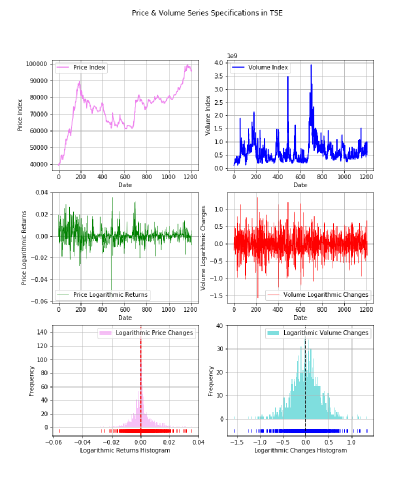
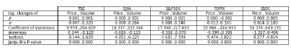
Figure 1: Descriptive statistics of investigated markets are demonstrated.

In Fig.1 top panel, the descriptive statistics for one of the markets is shown. Also, as illustrated in Fig.1 bottom panel, none of the time series are normally distributed. Hence, they are not monofractal [63]. Initially, after calculating the logarithmic changes of time series, they were standardized. Then

$$r_{price} = \ln{P_{t}}-\ln{P_{t-1}}$$

$$r_{volume} = \ln{V_{t}}-\ln{V_{t-1}},$$ (9)

where $t$ is daily data point, and also, $P$ and $V$ refer to price and trading volume, respectively. The above mentioned results are used as inputs to the methodology.

4 Empirical Results

MF-DXA

After detrending in each non-overlapping segments, $\nu$, with length of $s$ for price, volume, and price-volume cross series, we shall in order to estimate the power-law relation, compute $\log(F)-\log(s)$. This is illustrated in Fig. 2 for the markets we investigated. In Fig. 3 and Fig. 4, the multifractality features of price-volume coupling for the investigated markets are presented.

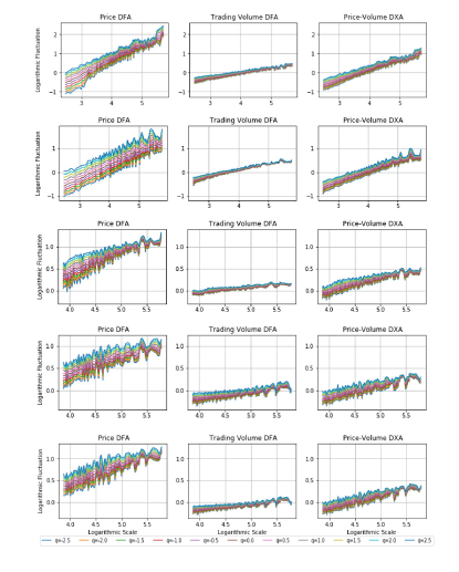
Figure 2: $log(F)-log(s)$ for price index (left) and trading volume (middle) and their cross correlation (right) are demonstrated. From top to bottom, $log(F)-log(s)$ for TSE, SSEC, TOPIX, S&P500, DJIA, are shown.

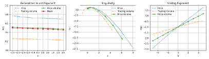
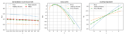
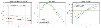
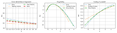
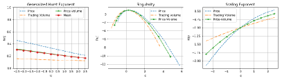
Figure 3: Multifractality features such as Hurst exponent spectrum for price index (left) and trading volume (middle) and their price-volume correlation (right) are demonstrated. From top to bottom, multifractality features of TSE, SSEC, TOPIX, S&P500, DJIA, are shown.

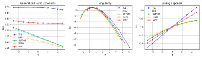
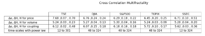
Figure 4: Top: Multifractality features of price-volume coupling: Hurst exponent spectrum (left), singularity spectrum (middle) and scaling exponent (right) are shown. Bottom: Multifractality features of price time series, volume time series, and price-volume coupling are presented.

Altering a power law relation in different time-scales, means there exists scale variance and it is an indication different power-laws are needed to describe the corresponding time-series in different time-scales. On the other hand, a system is scale invariant when it generates its structure in different intervals. To obtain valid power-laws, proper scales are extracted which are shown in Fig. 4. It is worthy to say that for window lengths near $N$, the local trend of the segments become more similar to the whole time series rather than the too small segments, and in this process $F(s)$ becomes relatively independent of iterations on $\nu$.
Another reason for this phenomenon is the effect size of variations. Large segments (small segments) contain large-scale (small-scale) behaviors of the time series. Hence, applying the $q$th-order effect on the fluctuation function, leads to a divergence of $\log(F)-\log(s)$ for small scales. Nevertheless, for $s\ll N$ (local deviation of detrended segments are small on relatively small scales), the fitting polynomial –a linear local trend in this study– is well fitted on the segments and results in a magnification of the divergence of $F(s)$ for different $q$ values.
The generalized Hurst exponent presents multifractality of correlations. Based on Podobnik and Stanley [10], the Binomial measure from the $p$-model for the cross-correlation exponent of the fractionally auto-regressive integrated moving average (FARIMA) with identical stochastic noises, is equal to their arithmetic mean at $q=2$. However, Zhou [59] illustrated that the same relation for $q$ values other than 2, is valid [15] which is presented in red color in the left panels in 3.

In Fig.3, price multifractalities of all investigated markets are larger than volume multifractalities of the corresponding markets. If the time series is multifractal and $q$ is extremely large for the system, it may yield to $f_{(\alpha)}<0$ [66]. On the other hand, $f_{(\alpha)}<0$, may occur on extremely large or small singularity spectra [9]. Since a negative dimension is an unreal solution, this may warn us that the timeseries histogram is spars– which is a characteristic of real-world financial timeseries due to the fact that they may not be Guassian. Hence, those events near the tails of the histogram increase and eliminate limited-length effects. In addition, the right panels of Fig. 3, which relate to the nonlinearity of scaling exponents, prove that price multifractalities occur more often than volume mulifractalities of the markets we investigated. As a result, the multifractality of price-volume coupling can be found to be between the corresponding price and trading volume multifractalities.
As shown in Fig. 4, among the investigated markets, TSE has the least multifractality degree of price-volume coupling. Conversely, for the developed markets, the multifractality degrees of price-volume coupling are large than that of emerging markets. However, considering the singularity spectrum, low efficiency of the markets contributes to high singularity strength in price-volume couplings. Furthermore, low efficiency in the markets coincides with a scaling exponent of price-volume coupling with low curvature. It is notable that, the price-volume coupling of the developed markets such as DJIA, S&P500 and TOPIX (with $H^{price}<0.5$), are highly affected by trading volume. Hence, their price-volume couplings are not a random walk (on the contrary to the TSE). What is noteworthy, is that the singularity spectrum for an emerging market such as TSE (with $H^{price}>0.5$) is more left-hooked than that of the developed ones. The price-volume cross correlation of an emerging market is more led by some attributes other than volume of transactions (such as the manipulation of the supply and demand at certain prices which causes markets to be led more by price rather than trading volume!). This is proven by the left panels of Fig.3.

Cross Correlation Coefficient

Firstly, by applying Eq. 8 the scales with significant cross correlation coefficients are distinguished, as shown in Fig. 5. After a statistical confirmation of correlation significance, by applying Eq. 9, we evaluate the scaling behavior of correlation coefficients of the investigated markets throughout different time-scales, Fig. 5, bottom.

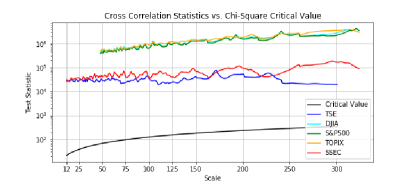
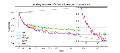
Figure 5: Top: Cross correlation statistics of the investigated market versus critical value are shown. Bottom: Scaling behavior of correlation coefficients of the investigated market are demonstrated.

We filtered the area with significant cross correlations in order to investigate the cross correlation coefficients in the next step. Fig. 5 contains cross correlation statistics versus critical value, and Fig. 5, bottom, shows the corresponding correlation coefficients in a multiscale pattern–all for $h_{(q=2)}$– of price-volume coupling for investigated markets. As shown, the cross correlation statistics are significant for the studied range of time-scales. As illustrated in Fig. 5, bottom, the large temporal segments size contribute to the small cross-correlation coefficients and large fluctuation functions (such as ${DFA}_{price}$, ${DFA}_{volume}$, ${DXA}_{price-volume}$). When it comes to the large scales, the multifractal behavior of fluctuation functions corresponding to price and volume, does not present an extreme correlation and the scaling behavior of price and trading volumes are totally different in relatively large scales. Hence, in large scales, it makes no sense to describe price volatilities by trading volume volatilities. It is noteworthy that, in Fig. 5, bottom, the price-volume cross correlations of domains maintaining a power law in both price time series and volume time series in each market, will show that the decrease of the correlation coefficient co-occurs faster by an increase of time-scales in the emerging markets such as TSE and SSEC rather than that of the developed ones. Consequently, as shown in Fig. 5 and Fig. 5, bottom, by increasing time-scale, the behavior of emerging markets deviate from the behavior of developed markets. In the period of our study, it is obvious that among all investigated markets, the scaling correlation coefficients of the developed markets maintain to 0.4 to around 0.6. On the other hand, the scaling correlation coefficients of the emerging markets maintain around less than 1 and ultimately tend to somehow 0.2 to 0.35 in large time-scales. It means that the decrease in scaling correlation coefficients of emerging markets is more sensitive rather than that of the developed markets toward time-scale size.

5 Conclusion

In multifractal time series, we need to consider several statistical moments to describe the behavior of the system. Therefore, investors need to execute a multifractal analysis to be more familiar with the system’s behavior. Nevertheless, in the aforementioned markets, the generalized Hurst exponent, $h_{(q)}$, is a function of q. By illustrating the singularity spectrum, this study shows nonlinear behavior of price, volume, and price-volume structure. As a consequence, studying a single variable without considering simultaneous collective effects and their cross effects, may be biased.

Since the Hurst exponent of price is larger than 0.5 ($h_{(q=2)}^{price}>0.5$) for TSE, it is an emerging market with persistent behavior of price volatilities. Conversely, because of $h_{(q=2)}^{price}<0.5$, DJIA, S&P500 and TOPIX, are classified as developed markets with short timescale and anti-persistent behavior. The investigated markets are affected by their memory. Hence, the models which analyze these markets based on the Efficient Market Hypothesis may no longer estimate the market behavior accurately. In an inefficient market, the short timescale and large timescale phenomena exist in price.
Long-range timescales leads to more predictability for price. Long-range behaviors cause more persistent information effects and lessen the speed of fading-out information from past dynamics. Furthermore, the trading volume volatilities present negatively correlated behavior. Furthermore, the multifractal behavior of volume DFA is less than that of price DFA.
Moreover, the cross correlation coefficients show scaling behaviors which are totally significant in the investigated time-scales and decreases by increasing time-scales.

Since for the price-volume coupling we have $0.5>H^{TSE}>H^{SSEC}>H^{developed}$, it can be concluded that the price-volume couplings for the investigated developed markets are significantly negatively correlated and they possess significant valid information. As a whole, in emerging markets, market behavior is guided more by a phenomenon other than trading volume rather than just trading volume.

Multifractal volatilities in financial markets have become highly important in risk management. Efficient risk management requires understanding of information translation between couplings of stock markets structures and internal and external dynamics. One of the most practical measures of this study is applying the cross correlation matrix based on Laloux et al. [67] and Plerou et al. [68] for several fluctuation functions to measure market risk.

References

- [1] T. Lux, M. Ausloos, Market fluctuations i: Scaling, multiscaling, and their possible origins, in: The Science of Disasters, Springer Berlin Heidelberg, 2002, pp. 372–409. doi:10.1007/978-3-642-56257-0_13.
- [2] C.-K. Peng, S. V. Buldyrev, S. Havlin, M. Simons, H. E. Stanley, A. L. Goldberger, Mosaic organization of DNA nucleotides, Physical Review E 49 (2) (1994) 1685–1689. doi:10.1103/physreve.49.1685.
- [3] C.-K. Peng, S. Havlin, H. E. Stanley, A. L. Goldberger, Quantification of scaling exponents and crossover phenomena in nonstationary heartbeat time series, Chaos: An Interdisciplinary Journal of Nonlinear Science 5 (1) (1995) 82–87. doi:10.1063/1.166141.
- [4] S. Shadkhoo, G. R. Jafari, Multifractal detrended cross-correlation analysis of temporal and spatial seismic data, The European Physical Journal B 72 (4) (2009) 679–683. doi:10.1140/epjb/e2009-00402-2.
- [5] L. Hedayatifar, M. Vahabi, G. R. Jafari, Coupling detrended fluctuation analysis for analyzing coupled nonstationary signals, Physical Review E 84 (2) (2011) 021138. doi:10.1103/physreve.84.021138.
- [6] S. Ossadnik, S. Buldyrev, A. Goldberger, S. Havlin, R. Mantegna, C. Peng, M. Simons, H. Stanley, Correlation approach to identify coding regions in DNA sequences, Biophysical Journal 67 (1) (1994) 64–70. doi:10.1016/s0006-3495(94)80455-2.
- [7] J. W. Kantelhardt, S. A. Zschiegner, E. Koscielny-Bunde, S. Havlin, A. Bunde, H. Stanley, Multifractal detrended fluctuation analysis of nonstationary time series, Physica A: Statistical Mechanics and its Applications 316 (1-4) (2002) 87–114. doi:10.1016/s0378-4371(02)01383-3.
- [8] R. Kavasseri, R. Nagarajan, A multifractal description of wind speed records, Chaos, Solitons & Fractals 24 (1) (2005) 165–173. doi:10.1016/s0960-0779(04)00533-8.
- [9] Z.-Q. Jiang, W.-X. Zhou, Scale invariant distribution and multifractality of volatility multipliers in stock markets, Physica A: Statistical Mechanics and its Applications 381 (2007) 343–350. doi:10.1016/j.physa.2007.03.015.
- [10] B. Podobnik, H. E. Stanley, Detrended cross-correlation analysis: A new method for analyzing two nonstationary time series, Physical Review Letters 100 (8) (2008) 084102. doi:10.1103/physrevlett.100.084102.
- [11] B. Podobnik, D. Horvatic, A. M. Petersen, H. E. Stanley, Cross-correlations between volume change and price change, Proceedings of the National Academy of Sciences 106 (52) (2009) 22079–22084. doi:10.1073/pnas.0911983106.
- [12] A. Lin, P. Shang, H. Zhou, Cross-correlations and structures of stock markets based on multiscale MF-DXA and PCA, Nonlinear Dynamics 78 (1) (2014) 485–494. doi:10.1007/s11071-014-1455-5.
- [13] Z.-Q. Jiang, W.-J. Xie, W.-X. Zhou, D. Sornette, Multifractal analysis of financial markets, arXiv preprint arXiv:1805.04750.
- [14] P. Caraiani, E. Haven, Evidence of multifractality from CEE exchange rates against euro, Physica A: Statistical Mechanics and its Applications 419 (2015) 395–407. doi:10.1016/j.physa.2014.06.043.
- [15] X. Zhuang, Y. Wei, B. Zhang, Multifractal detrended cross-correlation analysis of carbon and crude oil markets, Physica A: Statistical Mechanics and its Applications 399 (2014) 113–125. doi:10.1016/j.physa.2013.12.048.
- [16] S. Drożdż, R. Gȩbarowski, L. Minati, P. Oświȩcimka, M. Wactorek, Bitcoin market route to maturity? evidence from return fluctuations, temporal correlations and multiscaling effects, Chaos: An Interdisciplinary Journal of Nonlinear Science 28 (7) (2018) 071101. doi:10.1063/1.5036517.
- [17] H. Safdari, A. Hosseiny, S. V. Farahani, G. Jafari, A picture for the coupling of unemployment and inflation, Physica A: Statistical Mechanics and its Applications 444 (2016) 744–750. doi:10.1016/j.physa.2015.10.072.
- [18] S. Rendón de la Torre, J. Kalda, R. Kitt, J. Engelbrecht, Fractal and multifractal analysis of complex networks: Estonian network of payments, The European Physical Journal B 90 (12) (2017) 90–234. doi:10.1140/epjb/e2017-80214-5.
- [19] M. Ausloos, Statistical physics in meteorology, Physica A: Statistical Mechanics and its Applications 336 (1-2) (2004) 93–101. doi:10.1016/j.physa.2004.01.014.
- [20] K. Ivanova, N. Gospodinova, H. N. Shirer, T. P. Ackerman, M. A. Mikhalev, M. Ausloos, Multifractality of cloud base height profiles (2001). arXiv:cond-mat/0108395.
- [21] M. Ausloos, Generalized hurst exponent and multifractal function of original and translated texts mapped into frequency and length time series, Phys. Rev. E 86 (2012) 031108. doi:10.1103/PhysRevE.86.031108.
- [22] M. Ausloos, R. Cerqueti, C. Lupi, Long-range properties and data validity for hydrogeological time series: The case of the paglia river, Physica A: Statistical Mechanics and its Applications 470 (2017) 39–50. doi:10.1016/j.physa.2016.11.137.
- [23] M. S. Movahed, G. R. Jafari, F. Ghasemi, S. Rahvar, M. R. R. Tabar, Multifractal detrended fluctuation analysis of sunspot time series, Journal of Statistical Mechanics: Theory and Experiment 2006 (02) (2006) P02003–P02003. doi:10.1088/1742-5468/2006/02/p02003.
- [24] M. Ausloos, K. Ivanova, Mechanistic approach to generalized technical analysis of share prices and stock market indices, The European Physical Journal B - Condensed Matter 27 (2) (2002) 177–187. doi:10.1140/epjb/e20020144.
- [25] S. Nasiri, E. Bektas, G. Jafari, The impact of trading volume on the stock market credibility: Bohmian quantum potential approach, Physica A: Statistical Mechanics and its Applications 512 (2018) 1104–1112. doi:10.1016/j.physa.2018.08.026.
- [26] Y. Guo, J. Huang, H. Cheng, Multifractal features of metal futures market based on multifractal detrended cross-correlation analysis 41 (10) (2012) 1509–1525. doi:10.1108/03684921211276710.
- [27] G. meng Chen, M. Firth, O. M. Rui, The dynamic relation between stock returns, trading volume, and volatility, The Financial Review 36 (3) (2001) 153–174. doi:10.1111/j.1540-6288.2001.tb00024.x.
- [28] C.-C. Chuang, C.-M. Kuan, H.-Y. Lin, Causality in quantiles and dynamic stock return–volume relations, Journal of Banking & Finance 33 (7) (2009) 1351–1360. doi:10.1016/j.jbankfin.2009.02.013.
- [29] J. Y. Campbell, S. J. Grossman, J. Wang, Trading volume and serial correlation in stock returns, The Quarterly Journal of Economics 108 (4) (1993) 905–939. doi:10.2307/2118454.
- [30] M. Ahmad, A. Sarr, Joint distribution of stock market returns and trading volume, Rev. Integr. Bus. Econ. Res. 5 (2016) 110–116. doi:http://sibresearch.org/uploads/3/4/0/9/34097180/riber_b16-085_110-116.pdf.
-
[31]
M. F. M. Osborne, Brownian motion in
the stock market, Operations Research 7 (2) (1959) 145–173.
URL http://www.jstor.org/stable/167153 - [32] K. Saatcioglu, L. T. Starks, The stock price–volume relationship in emerging stock markets: the case of latin america, International Journal of Forecasting 14 (2) (1998) 215–225. doi:10.1016/s0169-2070(98)00028-4.
- [33] J. Wang, A model of competitive stock trading volume, Journal of Political Economy 102 (1) (1994) 127–168. doi:10.1086/261924.
- [34] W. Huang, K. Mazouz, Excess cash, trading continuity, and liquidity risk, Journal of Corporate Finance 48 (2018) 275–291. doi:10.1016/j.jcorpfin.2017.11.005.
- [35] S. Buldyrev, A. Goldberger, S. Havlin, R. N. Mantegna, M. Matsa, C. Peng, M. Simons, H. Stanley, Long-range correlation properties of coding and noncoding dna sequences: Genbank analysis, Phys. Rev. E 51 (1995) 5084–5091.
- [36] J. Barnes, D. Allan, A statistical model of flicker noise, Proceedings of the IEEE 54 (2) (1966) 176–178. doi:10.1109/proc.1966.4630.
- [37] M. S. Taqqu, V. Teverovsky, W. Willinger, ESTIMATORS FOR LONG-RANGE DEPENDENCE: AN EMPIRICAL STUDY, Fractals 03 (04) (1995) 785–798. doi:10.1142/s0218348x95000692.
- [38] J. W. Kantelhardt, E. Koscielny-Bunde, H. H. Rego, S. Havlin, A. Bunde, Detecting long-range correlations with detrended fluctuation analysis, Physica A: Statistical Mechanics and its Applications 295 (3-4) (2001) 441–454. doi:10.1016/s0378-4371(01)00144-3.
- [39] K. Hu, P. C. Ivanov, Z. Chen, P. Carpena, H. E. Stanley, Effect of trends on detrended fluctuation analysis, Physical Review E 64 (1) (2001) 011114. doi:10.1103/physreve.64.011114.
- [40] Z. Chen, P. C. Ivanov, K. Hu, H. E. Stanley, Effect of nonstationarities on detrended fluctuation analysis, Physical Review E 65 (4) (2002) 041107. doi:10.1103/physreve.65.041107.
- [41] J. Kwapień, S. Drożdż, Physical approach to complex systems, Physics Reports 515 (3-4) (2012) 115–226. doi:10.1016/j.physrep.2012.01.007.
- [42] H.-Y. Chen, C.-F. Lee, W. K. Shih, Technical, fundamental, and combined information for separating winners from losers, Pacific-Basin Finance Journal 39 (2016) 224–242. doi:10.1016/j.pacfin.2016.06.008.
- [43] A. M. Pece, N. Petria, Volatility, thin trading and non-liniarities: An empirical approach for the BET index during pre-crisis and post-crisis periods, Procedia Economics and Finance 32 (2015) 1342–1352. doi:10.1016/s2212-5671(15)01511-7.
- [44] S. R. Ozturk, M. van der Wel, D. van Dijk, Intraday price discovery in fragmented markets, Journal of Financial Markets 32 (2017) 28–48. doi:10.1016/j.finmar.2016.10.001.
- [45] K. Hong, E. Wu, The roles of past returns and firm fundamentals in driving us stock price movements, International Review of Financial Analysis 43 (C) (2016) 62–75.
- [46] H. Chan, P. Docherty, Momentum in australian style portfolios: risk or inefficiency?, Accounting & Finance 56 (2) (2015) 333–361. doi:10.1111/acfi.12106.
- [47] R. Dash, P. K. Dash, A hybrid stock trading framework integrating technical analysis with machine learning techniques, The Journal of Finance and Data Science 2 (1) (2016) 42–57. doi:10.1016/j.jfds.2016.03.002.
- [48] J. S. Abarbanell, B. J. Bushee, Fundamental analysis, future earnings, and stock prices, Journal of Accounting Research 35 (1) (1997) 1. doi:10.2307/2491464.
- [49] T. Jamali, G. R. Jafari, Spectra of empirical autocorrelation matrices: A random-matrix-theory–inspired perspective, EPL (Europhysics Letters) 111 (1) (2015) 10001. doi:10.1209/0295-5075/111/10001.
- [50] F. Tahmasebi, S. Meskinimood, A. Namaki, S. V. Farahani, S. Jalalzadeh, G. R. Jafari, Financial market images: A practical approach owing to the secret quantum potential, EPL (Europhysics Letters) 109 (3) (2015) 30001. doi:10.1209/0295-5075/109/30001.
- [51] B. Podobnik, Z.-Q. Jiang, W.-X. Zhou, H. E. Stanley, Statistical tests for power-law cross-correlated processes, Physical Review E 84 (6) (2011) 066118. doi:10.1103/physreve.84.066118.
- [52] H. Zhu, W. Zhang, Multifractal property of chinese stock market in the csi 800 index based on mf-dfa approach, Physica A: Statistical Mechanics and its Applications 490 (2018) 497–503. doi:10.1016/j.physa.2017.08.060.
- [53] A. Carbone, G. Castelli, H. Stanley, Time-dependent hurst exponent in financial time series, Physica A: Statistical Mechanics and its Applications 344 (1-2) (2004) 267–271. doi:10.1016/j.physa.2004.06.130.
- [54] R. N. Mantegna, H. E. Stanley, An Introduction to Econophysics: Correlations and Complexity in Finance, Cambridge: Cambridge University Press, 2000.
- [55] Y. Liu, P. Gopikrishnan, Cizeau, Meyer, Peng, H. E. Stanley, Statistical properties of the volatility of price fluctuations, Physical Review E 60 (2) (1999) 1390–1400. doi:10.1103/physreve.60.1390.
- [56] N. Vandewalle, M. Ausloos, P. Boveroux, A. Minguet, Visualizing the log-periodic pattern before crashes, The European Physical Journal B 9 (2) (1999) 355–359. doi:10.1007/s100510050775.
- [57] Y. Yin, P. Shang, Modified DFA and DCCA approach for quantifying the multiscale correlation structure of financial markets, Physica A: Statistical Mechanics and its Applications 392 (24) (2013) 6442–6457. doi:10.1016/j.physa.2013.07.070.
- [58] L. Zunino, B. Tabak, A. Figliola, D. Pérez, M. Garavaglia, O. Rosso, A multifractal approach for stock market inefficiency, Physica A: Statistical Mechanics and its Applications 387 (26) (2008) 6558–6566. doi:10.1016/j.physa.2008.08.028.
- [59] W.-X. Zhou, Multifractal detrended cross-correlation analysis for two nonstationary signals, Physical Review E 77 (6) (2008) 066211. doi:10.1103/physreve.77.066211.
- [60] A. Cottet, W. Belzig, C. Bruder, Positive cross correlations in a three-terminal quantum dot with ferromagnetic contacts, Physical Review Letters 92 (20) (2004) 206801. doi:10.1103/physrevlett.92.206801.
- [61] M. Campillo, Long-range correlations in the diffuse seismic coda, Science 299 (5606) (2003) 547–549. doi:10.1126/science.1078551.
- [62] S. Hajian, M. S. Movahed, Multifractal detrended cross-correlation analysis of sunspot numbers and river flow fluctuations, Physica A: Statistical Mechanics and its Applications 389 (21) (2010) 4942–4957. doi:10.1016/j.physa.2010.06.025.
- [63] F. Shayeganfar, S. Jabbari-Farouji, M. S. Movahed, G. R. Jafari, M. R. R. Tabar, Multifractal analysis of light scattering-intensity fluctuations, Physical Review E 80 (6). doi:10.1103/physreve.80.061126.
- [64] A. Y. Schumann, J. W. Kantelhardt, Multifractal moving average analysis and test of multifractal model with tuned correlations, Physica A: Statistical Mechanics and its Applications 390 (14) (2011) 2637–2654. doi:10.1016/j.physa.2011.03.002.
- [65] G. R. Jafari, P. Pedram, L. Hedayatifar, Long-range correlation and multifractality in bach’s inventions pitches, Journal of Statistical Mechanics: Theory and Experiment 2007 (04) (2007) P04012–P04012. doi:10.1088/1742-5468/2007/04/p04012.
- [66] B. B. Mandelbrot, Negative fractal dimensions and multifractals, Physica A: Statistical Mechanics and its Applications 163 (1) (1990) 306–315. doi:10.1016/0378-4371(90)90339-t.
- [67] L. Laloux, P. Cizeau, J.-P. Bouchaud, M. Potters, Noise dressing of financial correlation matrices, Physical Review Letters 83 (7) (1999) 1467–1470. doi:10.1103/physrevlett.83.1467.
- [68] V. Plerou, P. Gopikrishnan, B. Rosenow, L. A. N. Amaral, T. Guhr, H. E. Stanley, Random matrix approach to cross correlations in financial data, Physical Review E 65 (6) (2002) 066126. doi:10.1103/physreve.65.066126.