EdgeStereo: An Effective Multi-Task Learning Network for Stereo Matching and Edge Detection

Abstract

Recently, leveraging on the development of end-to-end convolutional neural networks (CNNs), deep stereo matching networks have achieved remarkable performance far exceeding traditional approaches. However, state-of-the-art stereo frameworks still have difficulties at finding correct correspondences in texture-less regions, detailed structures, small objects and near boundaries, which could be alleviated by geometric clues such as edge contours and corresponding constraints. To improve the quality of disparity estimates in these challenging areas, we propose an effective multi-task learning network, EdgeStereo, composed of a disparity estimation branch and an edge detection branch, which enables end-to-end predictions of both disparity map and edge map. To effectively incorporate edge cues, we propose the edge-aware smoothness loss and edge feature embedding for inter-task interactions. It is demonstrated that based on our unified model, edge detection task and stereo matching task can promote each other. In addition, we design a compact module called residual pyramid to replace the commonly-used multi-stage cascaded structures or 3-D convolution based regularization modules in current stereo matching networks. By the time of the paper submission, EdgeStereo achieves state-of-art performance on the FlyingThings3D dataset, KITTI 2012 and KITTI 2015 stereo benchmarks, outperforming other published stereo matching methods by a noteworthy margin. EdgeStereo also achieves comparable generalization performance for disparity estimation because of the incorporation of edge cues.

1 Introduction

Stereo matching and depth estimation from stereo images have a wide range of applications, including robotics schmid2013stereo , medical imaging nam2012application , remote sensing shean2016automated , 3-D computational photography barron2015fast and autonomous driving menze2015object . The main goal of stereo matching is to find corresponding pixels from two viewpoints, producing dense depth data in a cost-efficient manner. Given a rectified stereo pair, supposing a pixel $(x,y)$ in the left image has a disparity $d$, its corresponding point can be found at $(x-d,y)$ in the right image. Consequently, the depth of this pixel can be obtained by $\frac{fT}{d}$, where $f$ denotes the focal length and $T$ denotes the baseline distance between two cameras.

As a classical research topic for decades, stereo matching was traditionally formulated as a multi-stage optimization problem hirschmuller2005accurate ; zhang2007estimating with a popular four-step pipeline scharstein2002taxonomy including matching cost computation, cost aggregation, optimization and disparity refinement. For instance, the popular Semi-Global Matching (SGM) hirschmuller2005accurate adopted dynamic programming to optimize an energy function for a locally optimal matching cost distribution, followed by several post-processing functions. However, performance of the traditional stereo matching methods is severely limited by hand-crafted matching cost descriptors, and engineered energy function and optimization procedures.

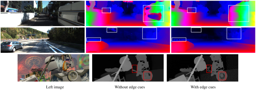
Figure 1: Examples of disparity estimates. From top to bottom: KITTI 2012, KITTI 2015 and FlyingThings3D datasets. From left to right: left image, disparity map from the disparity sub-network without edge cues, and disparity map from EdgeStereo. As shown in the boxes, disparity estimates are more accurate in ill-posed regions (reflective regions), detailed structures, and sky where ground-truth disparities don’t exist, after incorporating edge cues. (Better zoom in and view in color)

Recently, with the development of convolutional neural networks, stereo matching is cast as a learning task. Early CNN-based stereo matching methods zbontar2016stereo ; luo2016efficient mainly focused on representing image patches with powerful deep features then conducting matching cost computations. Significant gains are achieved compared with the traditional approaches, however most of these stereo networks have following limitations: 1) high computational burden from multiple forward passes for all potential disparities; 2) limited receptive field and the lack of context information to infer reliable correspondences in ill-posed regions; 3) still used post-processing functions which are hand-engineered with a number of empirically set parameters. Alternatively, the end-to-end disparity estimation networks seamlessly integrate all steps in the stereo matching pipeline for joint optimization mayer2016large , producing dense disparity maps from stereo images directly. 2-D encode-decoder structures with cascaded refinement pang2017cascade and regularization modules composed of 3-D convolutions kendall2017end are two of the most popular structures in current end-to-end stereo matching networks, which are demonstrated to be extremely effective for disparity estimation, benefitting from a large number of training data.

However, even the state-of-the-art end-to-end stereo networks may find it difficult to overcome local ambiguities in ill-posed regions, such as repeated patterns, textureless regions or reflective surfaces. Producing accurate disparity estimates is also challenging for detailed structures, small objects and near boundaries. Several end-to-end stereo networks kendall2017end ; chang2018pyramid enlarged their receptive fields through a stack of convolutional layers or spatial pooling modules, to encode context information for ill-posed regions where many potential correspondences exist. However, overlooking global context will inevitably lose high-frequency information that helps generate fine details in disparity maps. Moreover, without geometric constraints being utilized, most of these stereo matching networks are over-fitted, and corresponding generalization capabilities are poor.

Humans perform binocular alignment well at ill-posed regions by perceiving object boundaries in scenes, which is an important clue for detecting depth changes between background and foreground, and maintaining depth consistency for individuals. Consequently, combining semantic-meaningful edge cues provides beneficial geometric knowledge for stereo matching, meanwhile high-frequency feature representations are also supplemented for stereo networks with large receptive fields. For example, in Fig. 1, the disparity estimates in vehicle’s reflective surface, sky and image details are refined after incorporating edge cues.

This paper also asks a question, which has not been discussed by other CNN-based stereo methods yet, can stereo matching help other computer vision tasks through a unified convolutional neural network? In dense and high-quality disparity maps, the accurate depth boundary serves as an implicit but helpful geometric constraint for tasks like edge detection, semantic segmentation or instance segmentation etc. Considering the aforementioned problems in stereo matching, we intend to explore the mutual exploitation of stereo and edge information in a unified model, which is the main contribution of this paper.

Consequently, we design an effective multi-task learning network, EdgeStereo, that incorporates edge cues and corresponding regularization into the stereo matching pipeline. EdgeStereo consists of a disparity estimation branch and an edge detection branch, meanwhile two sub-networks share the shallow part of the backbone and low-level features. During training, interactions between the tasks are two-folds: firstly, the edge features are embedded into the disparity branch providing fine-grained representations; secondly, the edge map in the edge branch is utilized in our proposed edge-aware smoothness loss, which guides the multi-task learning in EdgeStereo. During testing, end-to-end predictions of both disparity map and edge map are enabled.

Basically, we first use ResNet he2016deep to extract image descriptors from a stereo pair and compute a cost volume by means of a correlation layer Dosovitskiy2015FlowNet . Then the concatenation of left image descriptor, matching cost volume and edge features are fed to a regularization module, to regress a full-size disparity map. In EdgeStereo, we design an hourglass structure composed of 2-D convolutions as the regularization module. Different from the decoder in DispNet mayer2016large , cascaded structures in pang2017cascade ; liang2017learning and 3-D convolution based regularization modules in kendall2017end ; chang2018pyramid , we propose a compact module called residual pyramid as the decoder for disparity regression. Some works use the same principle of residual pyramid for both optical flow sun2018pwc and stereo matching tonioni2019real . In residual pyramid, the disparities are directly estimated only at the smallest scale and the residual signals are predicted at other scales, hence making EdgeStereo an efficient one-stage model. Compared with other regularization modules, the proposed residual pyramid reduces the amount of parameters and improve the generalization capability as well as model interpretability. Finally, the produced disparity map and edge map are both optimized under the guidance of the edge-aware smoothness loss.

In EdgeStereo, the edge branch and disparity branch are both fully-convolutional so that end-to-end training can be conducted. Considering there is no dataset containing both edge annotations and ground-truth disparities, we propose an effective multi-stage training method. After multi-task learning, stereo matching task and edge detection task are both improved quantitatively and qualitatively. For stereo matching, EdgeStereo achieves the best performance on the FlyingThings3D dataset mayer2016large , KITTI 2012 geiger2012we and KITTI 2015 menze2015object stereo benchmarks compared with all published stereo methods. Particularly in the evaluation of “Reflective Regions” in the KITTI 2012 benchmark, EdgeStereo also outperforms other methods by a noteworthy margin. For edge detection, after the multi-task learning on a stereo matching dataset, edge predictions from EdgeStereo are improved, even if the stereo matching dataset does not contain ground-truth edge labels for training.

Our contributions and achievements are summarized below.

– We propose the multi-task learning network EdgeStereo that incorporates edge detection cues into the disparity estimation pipeline. For effective multi-task interactions, we design the edge feature embedding and propose the edge-aware smoothness loss. It is demonstrated that edge detection task and stereo matching task can promote each other based on our unified model. As far as we know, EdgeStereo is the first multi-task learning framework for stereo matching and edge detection.

– We design the residual pyramid, which is a compact decoder structure for disparity regression.

– Our method achieves state-of-the-art performance on the FlyingThings3D dataset, KITTI 2012 and KITTI 2015 stereo benchmarks, outperforming other stereo methods by a noteworthy margin. In addition, EdgeStereo is demonstrated with a comparable generalization capability for disparity estimation.

The rest of paper is organized as follows. After reviewing related work in Section 2, we introduce the overall architecture, residual pyramid and edge regularization in Section 3. Then in Section 4, we conduct detailed ablation studies to confirm the effectiveness of our design, and we compare EdgeStereo with other state-of-the-art stereo matching methods. Finally, Section 5 concludes the paper.

2 Related Work

2.1 Stereo Matching

Following the traditional stereo pipeline scharstein2002taxonomy , a great number of hand-engineered stereo matching methods have been proposed for matching cost computation geiger2010efficient ; heise2015fast , aggregation zhang2007estimating and optimization hirschmuller2005accurate ; kolmogorov2001computing ; klaus2006segment . Over the past few years, the convolutional neural network has been introduced to solve various problems in traditional stereo methods, and state-of-the-art performance is achieved. We hereby review stereo matching with emphasis placed on CNN-based methods, which can be roughly divided into three categories.

2.1.1 Non-end-to-end Stereo Matching

For non-end-to-end stereo methods, a CNN is introduced to replace one or more components in the legacy stereo pipeline. The first success of convolutional neural network for stereo matching was achieved by substituting hand-crafted matching cost with deep metrics. Zbontar and LeCun zbontar2015computing first introduced a deep siamese network to measure the similarity between two $9\times 9$ image patches. Luo et al. luo2016efficient accelerated matching cost calculation by an inner-product layer and proposed to learn a multi-label classification model over all possible disparities. Chen et al. chen2015deep proposed an embedding model fusing multi-scale features for matching cost calculation. Concurrently, Zagoruyko et al. zagoruyko2015learning investigated various CNN structures to compare image patches. In these methods, after obtaining a cost volume through a CNN, several non-learned post-processing functions are followed, including the cross-based cost aggregation, semi-global matching, left-right consistency check, sub-pixel enhancement and bilateral filtering mei2011building .

Besides the similarity measurement, deep neural networks could also be used in other sub-tasks. Gidaris et al. gidaris2016detect substituted hand-crafted disparity refinement functions with a three-stage network that detects, replaces and refines erroneous predictions. Shaked and Wolf shaked2016improved introduced an network pooling global information from a cost volume for initial disparity prediction. Seki et al. seki2017sgm raised the SGM-Net framework that predicts SGM penalties for regularization. Knobelreiter et al. knobelreiter2017end learned smoothness penalties through a CRF model for energy function optimization. In these methods, a number of hand-crafted regularization functions are still necessary to achieve comparable results.

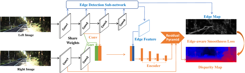
Figure 2: Overall architecture. EdgeStereo consists of a disparity estimation branch and an edge detection branch, sharing the shallow part of the backbone. Taking a fused representation as input, the regularization module (encoder and the residual pyramid) produces a full-size disparity map. To obtain disparity maps with fine details and conduct multi-task learning, edge cues are incorporated into the disparity branch by the edge feature embedding and edge-aware smoothness loss.

2.1.2 End-to-end Stereo Matching

Inspired by other pixel-wise labeling tasks, fully-convolutio-
nal networks (FCN) long2015fully were carefully designed to regress disparity maps from stereo inputs without post-processing. All components in the legacy stereo pipeline are combined for joint optimization. Mayer et al. mayer2016large proposed the first end-to-end disparity estimation network called DispNet, in which an 1-D correlation layer was proposed for the cost calculation, and an encoder-decoder structure with shor-tcut connections ronneberger2015u was designed for disparity regression. They also released a large synthetic stereo matching dataset, making it possible to pretrain an end-to-end stereo matching network without over-fitting. Based on DispNet, Pang et al. pang2017cascade proposed a two-stage architecture called cascade residual learning (CRL) where the first stage gives initial predictions, and the second stage learns residuals. Liang et al. liang2017learning extended DispNet and designed a different disparity refinement sub-network, in which two stages are combined for joint learning based on the feature constancy.

Different from DispNet and its variants, Kendall et al. kendall2017end raised GC-Net in which the feature dimension is not collapsed when constructing a cost volume, and 3-D convolutions are used to regularize the cost volume and incorporate more context from the disparity dimension. Inspired by GC-Net, Chang et al. chang2018pyramid employed a spatial pyramid pooling module to extract multi-scale representations and designed a stacked 3-D CNN for cost volume regularization. Tulyakov et al. designed a practical deep stereo (PDS) network tulyakov2018practical where memory footprint is reduced by compressing concatenated image descriptors into compact representations before feeding to the 3-D regularization module.

Several end-to-end stereo methods focused on designing specific functional modules. Lu et al. lu2018sparse introduced an efficient stereo matching method based on their proposed sparse cost volume. Yu et al. yu2018deep proposed a two-stream architecture for better generation and selection of cost aggregation proposals from cost volumes. Jie et al. jie2018left proposed a left-right comparative recurrent (LRCR) model for stereo matching, which is the first end-to-end network that incorporates left-right consistency check into disparity regression using stacked convolutional LSTM.

Our method also enables end-to-end predictions of full-size disparity maps. Rather than regressing disparities from multi-stage cascaded structures or 3-D convolution based regularization modules, which makes stereo networks over-parameterized, EdgeStereo is an efficient one-stage network with better model interpretability because of the proposed residual pyramid.

2.1.3 Unsupervised Stereo Matching

Over the past few years, based on spatial transformation and view synthesis, several unsupervised learning methods were proposed for stereo matching without the need of ground-truth disparities during training. Tonioni et al. tonioni2017unsupervised propose a novel unsupervised adaptation approach that enables to finetune a deep learning stereo model without any ground-truth. Based on GC-Net, Zhong et al. zhong2017self proposed an unsupervised self-adaptive stereo matching network under the guidance of photometric errors. Zhou et al. zhou2017unsupervised presented an unsupervised framework to learn matching costs iteratively, supervised by a left-right consistency loss.

The view-synthesis based unsupervised stereo matching can also be adapted to unsupervised monocular depth estimation. Garg et al. garg2016unsupervised proposed the first unsupervised network for single-view depth estimation, in which per-pixel disparity is learned driven by an image reconstruction loss in a calibrated stereo environment. Based on garg2016unsupervised , Godard et al. godard2017unsupervised developed a fully-differentiable structure for photometric error minimization and designed a left-right disparity consistency term for regularization. Kuznietsov et al. kuznietsov2017semi proposed a semi-supervised approach where ground-truth depths and unsupervised binocular alignment losses are both used to train the monocular depth estimation network.

Although unsupervised methods get rid of the dependence on ground truth disparities, they are still not comparable with supervised methods (Our EdgeStereo). In addition, in unsupervised stereo networks, various smoothness terms were designed to regularize disparity maps. However, these image gradient based regularization terms are not robust and are inferior to our proposed edge-aware smoothness loss, as demonstrated in Section 4.

2.2 Edge Detection

Edge detection is a classical low-level vision task. Early methods focused on designing hand-engineered descriptors using low-level cues such as intensity and gradient canny1986computational ; dollar2006supervised , then employing sophisticated learning paradigm for classification dollar2015fast . Recently, inspired by FCN long2015fully , Xie et al. xie2015holistically designed the first end-to-end edge detection network called holistically-nested edge detector (HED), in which all output layers in side branches are connected to aggregate coarse-to-fine predictions for a final output. Liu et al. liu2016learning achieved some improvements compared with HED by employing relaxed labels to guide the training process. Liu et al. liu2017richer modified the network structure of HED, combining all meaningful convolutional features in the backbone for prediction. Since the structures of these fully-convolutional edge detection networks are concise and efficient, we propose a similar edge detection sub-network in our unified model, providing semantic-meaningful edge features and geometric constraints for stereo matching.

2.3 Deep Multi-task Network

Kendall et al. kendall2018multi propose a multi-task learning model learning per-pixel depth regression, semantic and instance segmentation from a monocular input image. Ramirez et al. ramirez2018geometry propose a semi-supervised framework aimed at joint semantic segmentation and depth estimation. Cheng et al. cheng2017segflow proposed an end-to-end architecture called SegFlow, which enables the joint learning of video object segmentation and optical flow. This model consists of a FCN long2015fully based segmentation branch and a FlowNet Dosovitskiy2015FlowNet based flow branch, in which feature maps of two tasks are concatenated and two branches are trained alternately. However, this multi-task architecture requires the dataset containing all types of ground-truth labels for different tasks during training, which limits its adaptation ability to other tasks. Mao et al. mao2017can also proposed a multi-task network called HyperLearner to help pedestrian detection. Diverse features from different tasks, such as semantic segmentation and edge detection etc, provide various representations which are concatenated with the backbone pedestrian detection network. However, multi-task learning is not conducted in this architecture because losses in the detection branch could not be propagated back to other branches, meanwhile geometric knowledge from other tasks is not fully exploited. With a similar motivation to ours, Yang et al. yang_segstereo proposed a unified model called SegStereo for semantic segmentation and disparity estimation, in which semantic features are utilized and a semantic softmax loss is introduced to improve the quality of disparity estimates especially in texture-less regions. However, in SegStereo, disparity estimation could not help semantic segmentation, and incorporating high-level semantic cues causes the loss of high-frequency information.

In this paper, we incorporate edge cues into the disparity estimation pipeline obtaining a unified multi-task learning architecture. The embedded edge features provide semantic-meaningful and high-frequency representations, meanwhile the proposed edge-aware smoothness loss carries beneficial geometric constraints for effective multi-task learning. In addition, the training dataset is not required to contain all types of ground-truth labels for different tasks. Comparisons with our previous work song2018stereo can be found in Section 4.7. Our latest EdgeStereo model achieves state-of-the-art performance on the FlyingThings3D, KITTI 2012 and KITTI 2015 datasets, outperforming all published stereo matching methods.

3 Approach

We present EdgeStereo, which is an effective multi-task learning network for stereo matching and edge detection. We would like to learn an optimal mapping from a stereo pair to a disparity map and an edge map corresponding to the reference image. However, we do not intend to design a machine learning model acting as a complete black box. Hence we develop several differentiable modules representing major components in the stereo matching pipeline, meanwhile leveraging geometric knowledge from edge detection.

In this section, we first present the basic network architecture of EdgeStereo. Then we introduce a key module for disparity regression: residual pyramid. Next we detail the incorporation strategies of edge cues, including the edge feature embedding and edge-aware smoothness loss. Furthermore we show how to conduct multi-task learning through the proposed multi-stage training method. Finally we introduce the detailed structure of EdgeStereo and give a layer-by-layer definition.

3.1 Basic Network Architecture

The overall architecture of EdgeStereo is shown in Fig. 2, in which two branches share the shallow part of the backbone. For the disparity branch, instead of using multiple networks for different components, we combine all modules into a single network composed of extraction, matching and regularization modules. In addition, we propose the residual pyramid so that disparity refinement is not required, making EdgeStereo an efficient one-stage architecture.

The extraction module outputs the image descriptors $\mathbb{F}^{l}$ and $\mathbb{F}^{r}$ carrying local semantic features for left and right images through the shared backbone. Then the matching module performs an explicit correlation operation using the 1-D correlation layer from Dosovitskiy2015FlowNet , capturing coarse correspondences between two descriptors for each potential disparity. Then the cost volume $\mathbb{F}_{c}$ is obtained. To preserve detailed information in the left image descriptor, we apply a convolutional block on $\mathbb{F}^{l}$ obtaining the refined representation $\mathbb{F}_{r}^{l}$.

The edge branch shares shallow layer representations with the disparity branch, meanwhile remaining convolutional features in the backbone are used to produce edge features and a semantic-meaningful edge map of the left image. Similarly, we also apply a convolutional block and obtain the transformed edge features $\mathbb{F}_{e}^{l}$. The left image descriptor $\mathbb{F}_{r}^{l}$, cost volume $\mathbb{F}_{c}$ and transformed edge features $\mathbb{F}_{e}^{l}$ are concatenated as the hybrid feature representation $\mathbb{F}_{h}$, which is referred to as edge feature embedding.

The regularization module takes $\mathbb{F}_{h}$ as input, regularizes it and produces a dense disparity map. This module is usually implemented as an hourglass structure with shortcut connections between encoder and decoder. We design a 2-D convolution based encoder different from existing encoder structures mayer2016large ; pang2017cascade ; liang2017learning , in which the residual block in ResNet he2016deep is adopted as the basic block for better information flow. Furthermore, we design the residual pyramid as the decoder, where shortcut connections are not required and a coarse-to-fine learning mechanism is employed. In the residual pyramid, which takes the sub-sampled hybrid feature representation as input, disparities are directly regressed only at the smallest scale and residual signals are predicted for refinement at other scales. The smallest scale of disparity estimates is not fixed, which can be specified by applying several deconvolutional blocks on the encoder. Finally, disparity and residual learning are regularized across multiple scales in the residual pyramid, guided by the edge-aware smoothness loss .

3.2 Residual Pyramid

For disparity refinement, existing methods gidaris2016detect ; pang2017cascade ; liang2017learning cascaded additional networks on the initial disparity prediction network, learning multi-scale residual signals. However, these cascaded structures that model the joint space of multiple networks are over-parameterized. In addition, the initial full-size disparity estimates are quite accurate in ordinary areas, but residual learning without geometric constraints is not easy in ill-posed regions, leading to approximately zero residual signals.

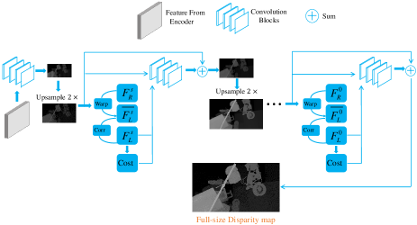
Figure 3: Overview of the residual pyramid. Disparities are directly estimated only at the smallest scale and residual signals are produced at other scales for refinement, making EdgeStereo an efficient one-stage architecture. Convolutional blocks are adopted to produce initial disparities and residual signals.

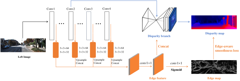
Figure 4: Overview of the edge branch. To preserve subtle details, fine-grained edge features are supplemented, meanwhile the edge-aware smoothness loss imposes beneficial object-level constraints on disparity training and multi-task learning.

To alleviate the aforementioned problems, we adopt the coarse-to-fine residual learning mechanism, and propose the residual pyramid that enables learning and refining disparities in a single decoder. In general, estimating disparities at the smallest scale is easier since the searching range is narrow, meanwhile significant areas are emphasized and less details are required. Therefore the initial disparity estimate acts as a good starting point. To obtain an up-sampled disparity map with extra details, we continuously predict residual signals at other scales, utilizing high-frequency representations and beneficial geometric constraints from edge cues. In addition, the coarse-to-fine residual learning mechanism benefits the overall training and alleviates the problem of over-fitting.

The structure of the residual pyramid is flexible. The number of scales $S$ in the residual pyramid is dependent on the total sub-sampling factor of the input volume. The disparity map at the smallest scale is denoted as $d_{S-1}$ ($\frac{1}{2^{S-1}}$ of the full size), then it is continuously up-sampled and refined with the residual signal $r_{s}$ at scale $s$, until the full-size disparity map $d_{0}$ is obtained. As shown in Eq. (1), $u(\cdot)$ denotes up-sampling by a factor of $2$ and $s$ denotes the scale.

$$\\ \\ d_{s}=u(d_{s+1})+r_{s},\,0\leq s<S\$$ (1)

Existing encoder-decoder structures pang2017cascade ; liang2017learning ; chang2018pyramid ; kendall2017end rely on shortcut connections to fuse high-level and fine-grained representations, which complicates the feature space of disparity regularization and makes stereo networks less explainable. Conversely we leverage the knowledge from stereo geometry and geometric constraints from edge cues to learn residuals, without the need for shortcut connections for direct disparity regression. As shown in Fig. 3, to predict the residual signal at scale $s$, we first use the up-sampled disparity map $u(d_{s+1})$ to warp the right image features $F_{R}^{s}$ at scale $s$ in the backbone, obtaining the synthesised left image features $\overline{F_{L}^{s}}$. Then we perform 1-D correlation between the synthesised and real left image features $F_{L}^{s}$, obtaining a cost volume $cost$ that characterizes left-right feature consistency based on existing disparity estimates $u(d_{s+1})$. We use feature representations rather than raw pixel intensities for binocular warping, because they are more robust to photometric appearances and can encode local context information. Finally, the concatenation of the left image features $F_{L}^{s}$, up-sampled disparity map $u(d_{s+1})$ and cost volume $cost$ are processed by several convolutional blocks, producing the residual signal $r_{s}$. At each scale, residuals are explicitly supervised by the edge-aware smoothness loss and the difference between disparity estimates and ground-truth labels, learning sharp transitions at object boundaries.

3.3 Incorporation of Edge Cues

As shown in Fig. 1, the disparity estimation sub-network without edge cues works well in ordinary areas, where matching clues can be easily captured. However, accurate predictions for detailed structures are not given due to the lack of fine-grained representations in the deep stereo network. In addition, disparity estimates in reflective regions and near boundaries are not accurate due to the lack of geometric knowledge and constraints. Hence we incorporate edge cues to regularize the disparity learning, as shown in Fig. 4.

The first incorporation of edge cues is the edge feature embedding. After the extraction module and matching module, the transformed edge features $\mathbb{F}_{e}^{l}$ are concatenated with the left image descriptor $\mathbb{F}_{r}^{l}$ and cost volume $\mathbb{F}_{c}$ before fed to the regularization module. Advantages are: 1) The cooperated edge branch shares the efficient computation and effective representations with the disparity branch; 2) The edge features $\mathbb{F}_{e}^{l}$ supplement fine-grained representations from image details and boundaries, bringing beneficial scene priors to the regularization module; 3) The aggregation of feature maps from different tasks facilitates the multi-task interactions during training.

The second incorporation of edge cues is the proposed edge-aware smoothness loss, denoted as $L_{sm}$. We encourage smooth disparity estimates in local neighborhoods and the loss term penalizes drastic depth changes in flat regions. To allow for depth discontinuities at object boundaries, previous methods Godard2016Unsupervised ; zhong2017self weight smoothness regularization terms based on the image gradient which is not robust to various photometric appearances. Differently, we raise the edge-aware smoothness loss based on the edge map gradient from the edge detection sub-network, which is more semantic-meaningful than the variation of raw pixel intensities. As shown in Eq. (2), where $N$ denotes the number of valid pixels, $\partial d$ denotes the disparity gradient, $\partial\mathcal{E}$ denotes the edge map gradient and the hyper-parameter $\beta$ controls the intensity of this smoothness regularization term.

$$\\ \\ L_{sm}=\frac{1}{N}\sum_{i,j}|\partial_{x}d_{i,j}|e^{-\beta|\partial_{x}\mathcal{E}_{i,j}|}+|\partial_{y}d_{i,j}|e^{-\beta|\partial_{y}\mathcal{E}_{i,j}|}$$ (2)

The edge-aware smoothness loss also facilitates the multi-task learning in EdgeStereo. During training, the edge-aware smoothness loss is propagated back to the disparity branch and edge branch. The disparity estimates and edge predictions are improved simultaneously, until sharp disparities and fine edge predictions are obtained. The regularization term utilizes the geometric prior that depth boundaries in a disparity map should be consistent with edge contours in the scene, which imposes beneficial object-level constraints on disparity training and multi-task learning.

The experiments in Section 4 demonstrate that incorporating edge cues can effectively help disparity estimation in detailed structures, reflective regions and near boundaries. In addition, edge predictions are also improved after the multi-task learning on a stereo matching dataset, even if edge annotations are not provided for training.

Table 1: Layers in EdgeStereo_RP_2. K means kernel size, S means stride, I/O means input/ouput channels. “,” means concat and “+” means element-wise summation.

Type	Layer	K	S	c I/O	Input	Resolution
1. Extraction Module
Conv	conv1_1a	3	2	3/64	left image	1/2
	conv1_1b				right image
Conv	conv1_2a	3	1	64/64	conv1_1a	1/2
	conv1_2b				conv1_1b
Conv	conv1_3a	3	1	64/128	conv1_2a	1/2
	conv1_3b				conv1_2b
2. Edge Detection Sub-network
Pooling	max_pool1	3	2	128/128	conv1_3a	1/4
ResNet50	conv2_1→conv2_3	3	1	128/256	max_pool1	1/4
ResNet50	conv3_1→conv3_4	3	2	256/512	conv2_3	1/8
ResNet50	conv4_1→conv4_6	3	1	512/1024	conv3_4	1/8
Conv	conv1_3_edge_1	3	1	128/64	conv1_3a	1/2
Conv	conv1_3_edge	3	1	64/32	conv1_3_edge_1	1/2
Conv	conv2_3_edge_1	3	1	256/64	conv2_3	1/4
Conv	conv2_3_edge	3	1	64/32	conv2_3_edge_1	1/4
Interp	conv2_3_edge_i	-	2	-	conv2_3_edge	1/2
Conv	conv3_4_edge_1	3	1	512/64	conv3_4	1/8
Conv	conv3_4_edge	3	1	64/32	conv3_4_edge_1	1/8
Interp	conv3_4_edge_i	-	4	-	conv3_4_edge	1/2
Conv	conv4_6_edge_1	3	1	1024/64	conv4_6	1/8
Conv	conv4_6_edge	3	1	64/32	conv4_6_edge_1	1/8
Interp	conv4_6_edge_i	-	4	-	conv4_6_edge	1/2
Conv	conv_edge	1	1	128/128	conv1_3_edge,conv2_3_edge_i,	1/2
					conv3_4_edge_i,conv4_6_edge_i
Conv	edge_score (no BN/ReLU)	1	1	128/1	conv_edge	1/2
Sigmoid	edge_map	-	-	-	edge_score	1/2
3. Matching Module and Edge Feature Embedding
Conv	conv_trans_a	3	1	128/128	conv1_3a	1/2
	conv_trans_b				conv1_3b
Corr	Corr_1d	-—	-—	128/97	conv_trans_a	1/2
					conv_trans_b
Pooling	pool_corr	3	2	225/225	conv_trans_a,Corr_1d	1/4
Conv	conv_edge_trans	3	2	128/64	conv_edge	1/4
Concat	hybrid_feature	-	-	/289	pool_corr,conv_edge_trans	1/4
4. Encoder
ResBlock	res2_1→res2_3	3	1	289/256	hybrid_feature	1/4
ResBlock	res3_1→res3_4	3	2	256/512	res2_3	1/8
ResBlock	res4_1→res4_6	3	1	512/1024	res3_4	1/8
ResBlock	res5_1→res5_3	3	1	1024/2048	res4_6	1/8
Conv	disp_conv5_4	3	1	2048/512	res5_3	1/8
5. Decoder and Residual Pyramid
Deconv	disp_deconv1	3	2	512/256	disp_conv5_4	1/4
Deconv	disp_deconv2	3	2	256/128	disp_deconv1	1/2
Conv	disp_conv6	3	1	128/32	disp_deconv2	1/2
Conv	disp_2 (no BN/ReLU)	3	1	32/1	disp_conv6	1/2
Deconv	disp_ref_a	3	2	128/32	conv1_3a	1
	disp_ref_b				conv1_3b
Interp	up_disp_2	-	2	-	disp_2	1
Warp	w_disp_ref_a	-—	-—	32/32	disp_ref_b	1
					up_disp_2
Corr	Corr_1d_res	-—	-—	32/21	disp_ref_a	1
					w_disp_ref_a
Conv	disp_res_conv1_1	1	1	54/64	Corr_1d_res,up_disp_2,disp_ref_a	1
Conv	disp_res_conv1_2	3	1	64/64	disp_res_conv1_1	1
Conv	disp_res_conv1_3	3	1	64/32	disp_res_conv1_2	1
Conv	disp_res_1 (no BN/ReLU)	3	1	32/1	disp_res_conv1_3	1
Sum	disp_1	-	-	-	up_disp_2+disp_res_1	1

3.4 Multi-stage Training Method and Objective Function

Considering there is no dataset containing both ground-truth disparities and edge annotations, in order to conduct effective multi-task learning in EdgeStereo , we propose a multi-stage training method where training is split into three stages. Weights of the shallow part of the backbone that two tasks share are fixed in all three stages.

In the first stage, the edge detection branch is trained on an edge detection dataset, guided by the class-balanced per-pixel binary cross-entropy loss proposed in liu2017richer .

In the second stage, we supervise disparities across $S$ scales in the residual pyramid on a stereo matching dataset. Deep supervision is adopted, forming the total loss as $C=\sum_{s=0}^{S-1}C_{s}$ where $C_{s}$ denotes the loss at scale $s$. Besides the edge-aware smoothness loss, we adopt the $L1$-loss $L_{r}$ as the disparity regression loss for supervised learning, as shown in Eq. (3).

$$\\ \\ L_{r}=\frac{1}{N}{||\,d-\hat{d}\,||}_{1}\,,$$ (3)

where $\hat{d}$ denotes the ground truth disparity. Hence the loss at scale $s$ becomes $C_{s}=\lambda_{r}^{s}L_{r}^{s}+\lambda_{sm}^{s}L_{sm}^{s}$, where $\lambda_{r}^{s}$ and $\lambda_{sm}^{s}$ are the loss weights for the edge-aware smoothness loss and disparity regression loss at scale $s$ respectively. In addition, weights in the edge branch are fixed in the second stage.

In the third stage, all layers in EdgeStereo except the shared backbone are optimized on the same stereo matching dataset used in the second stage. We adopt the same deep supervision strategy as stage two and conduct effective multi-task learning.

3.5 Model Specifications

The backbone network is ResNet-50 he2016deep . The shallow part that two tasks share is conv1_1 to conv1_3 in the ResNet-50 backbone. Hence the extracted unary features $\mathbb{F}^{l}$ and $\mathbb{F}^{r}$ are of $1/2$ spatial size to the raw image. In the matching module, the max displacement in the 1-D correlation layer (unidirectional, leftward) is set to $96$ hence the channel number of the cost volume $\mathbb{F}_{c}$ is $97$.

For the edge detection branch in EdgeStereo, we design a fully-convolutional sub-network similar to HED xie2015holistically , while the semantic-meaningful edge features are easier to obtain in our architecture. As shown in Fig. 4, we introduce four side branches, concatenate and fuse feature representations in all side branches, obtaining the edge features for embedding. Through another $1\times 1$ convolutional layer and a sigmoid layer, an edge map is produced, in which the edge probability is given for each pixel. The edge branch uses the ResNet-50 backbone from conv1_1 to conv4_6 and four side branches start from conv1_3, conv2_3, conv3_4 and conv4_6 respectively. In addition, each side branch consists of two $3\times 3$ convolutional blocks and a bilinear interpolation layer.

Taking the hybrid feature representation $\mathbb{F}_{h}$ as input, the disparity encoder contains $16$ residual blocks, similar to the structure of ResNet-50 from conv2_3 to conv5_3. Several convolutional layers in residual blocks are replaced with dilated convolutional layers zhao2017pyramid to integrate wider context information, hence the sub-sampled hybrid feature representation $\mathbb{F}_{d}$ from the encoder is of $1/8$ size.

As mentioned above, the structure of the residual pyramid is flexible. Depending on the smallest scale of disparity estimates, there are three different residual pyramids, denoted as $RP\_2$, $RP\_4$ and $RP\_8$ respectively: for $RP\_2$, two $3\times 3$ deconvolutional blocks with stride two are applied on $\mathbb{F}_{d}$, hence the initial disparity map is of $1/2$ size and only full-size residual signals are required; for $RP\_4$, one $3\times 3$ deconvolutional block with stride two is applied; for $RP\_8$, no deconvolutional block is applied hence the initial disparity map is of $1/8$ size. At each scale in the residual pyramid, three $3\times 3$ convolutional blocks and a convolutional layer with a single output are adopted to regress disparities or residual signals.

Finally, we present a detailed layer-by-layer definition of EdgeStereo_RP_2, which denotes the EdgeStereo model with the residual pyramid $RP\_2$. As shown in Table 1, each convolutional or deconvolutional block contains a convolutional or deconvolutional layer, a batch normalization layer and a ReLU layer, “Interp” denotes the bilinear interpolation layer, “ResNet50” denotes a part of the ResNet-50 backbone, and “ResBlock” denotes the residual blocks in the encoder.

4 Experiments

The experimental settings and results are provided. We first conduct detailed ablation studies to verify our design choices in EdgeStereo, meanwhile we also demonstrate that stereo matching task and edge detection task can promote each other based on our unified model. Then we compare EdgeStereo with other state-of-the-art stereo matching methods on the FlyingThings3D dataset mayer2016large , KITTI 2012 geiger2012we and KITTI 2015 menze2015object stereo benchmarks. Finally, we prove that our EdgeStereo has a comparable generalization capability for disparity estimation because of the incorporation of edge cues.

4.1 Datasets and Evaluation Metrics

4.1.1 Datasets

Five publicly available stereo matching datasets are adopted for training and testing in EdgeStereo.

(i) FlyingThings3D mayer2016large : a large-scale synthetic dataset with dense ground-truth disparities, containing $22390$ stereo pairs for training and $4370$ pairs for testing. This virtual dataset contains some unreasonably large disparities; hence two specific testing protocols are widely used: Protocol 1, following CRL pang2017cascade , if more than $25\%$ of disparity values in the ground-truth disparity map are greater than $300$, the corresponding stereo pair is removed; Protocol 2, following PSMNet chang2018pyramid , we only calculate errors for pixels whose ground-truth disparity $<192$. We adopt both protocols for fair comparison with other state-of-the-art stereo matching methods.

(ii) KITTI2012 geiger2012we : a real-world dataset with still street views from a driving car. It contains $194$ stereo pairs for training with sparse ground-truth disparities and $195$ testing pairs without ground-truth. We further divide the whole training data into a training set ($160$ pairs) and a validation set ($34$ pairs) .

(iii) KITTI2015 menze2015object : a real-world dataset with dynamic street views. It contains $200$ training pairs and $200$ testing pairs. We divide the whole training data into a training set ($160$ pairs) and a validation set ($40$ pairs), following luo2016efficient .

(iv) CityScapes cordts2016cityscapes : an urban scene understanding dataset. This dataset provides $19997$ rectified stereo pairs and their disparity maps pre-computed by the SGM algorithm hirschmuller2005accurate in the extra training set. As illustrated in yang2018srcdisp , combining synthetic and realistic data for pretraining is helpful. Hence we fuse the data in the extra training set of CityScapes with the training data in FlyingThings3D for EdgeStereo pretraining.

(v) Middlebury 2014 scharstein2014high : a small in-door dataset containing $15$ training pairs with dense ground-truth disparities and $15$ test pairs.

Two publicly available edge detection datasets are adopted for training and testing in EdgeStereo.

(i) Multicue mely2016systematic : a boundary and edge detection dataset with challenging natural scenes. All $100$ images are used for training. We mix the augmentation data of Multicue with the PASCAL VOC Context dataset mottaghi2014role , to pretrain the edge detection sub-network in EdgeStereo.

(ii) BSDS500 arbelaez2011contour : a widely used edge detection dataset composed of $200$ training, $100$ validation and $200$ testing images. We only use this dataset for testing.

4.1.2 Metrics

For stereo matching evaluation, we adopt the end-point-error (EPE) which measures the average Euclidean distance between ground-truth and disparity estimate. We also calculate the percentage of pixels whose EPE is larger than $t$ pixels, denoted as $t$-pixel error ($>t\,px$).

For edge detection evaluation, we adopt two widely used metrics: F-measure ($\frac{2*Precision*Recall}{Precision+Recall}$) of optimal dataset scale (ODS), and F-measure of optimal image scale (OIS).

Table 2: Ablation study of edge cues and the comparison of different smoothness losses for stereo matching. For evaluation, we compute $3$-pixel error (%) and EPE on the FlyingThings3D test set (disparity $<192$), KITTI 2012 and 2015 validation sets.

Model	FlyingThings3D		KITTI 2012 val		KITTI 2015 val
	$>3\,px$	EPE	$>3\,px$	EPE	$>3\,px$	EPE
1. Basic ablation study
Baseline model (without edge cues)	4.443	0.840	2.844	0.606	3.192	0.770
Baseline with edge-aware smoothness loss	4.103	0.788	2.555	0.568	3.011	0.754
Baseline with edge feature and edge-aware smoothness loss	3.940	0.751	2.385	0.555	2.839	0.729
2. Comparison of smoothness loss regularization
EdgeStereo with Charbonnier smoothness loss yang_segstereo	3.971	0.756	2.852	0.691	3.024	0.769
EdgeStereo with second-order gradient smoothness loss zhong2017self	4.074	0.790	2.816	0.646	3.158	0.783
EdgeStereo (edge-aware smoothness loss)	3.940	0.751	2.385	0.555	2.839	0.729

4.2 Implementation Details

We implement EdgeStereo based on Caffe jia2014caffe . The ResNet-50 model pre-trained on ImageNet deng2009imagenet is adopted to initialize our network. The training is conducted on eight Nvidia GTX 1080Ti GPUs.

In the first training stage, we fuse the Multicue dataset with PASCAL VOC Context dataset to pretrain the edge branch. We adopt the stochastic gradient descent (SGD) with a minibatch of $16$ images. The initial learning rate is set to $0.01$ and divided by $10$ every $10K$ iterations. We set the momentum to $0.9$ and weight decay to $0.0002$. We run SGD for $40K$ iterations totally in the first stage. For data augmentation, we rotate the images in Multicue to $4$ different angles ($0$, $90$, $180$ and $270$ degrees) and flip them at each angle, and we also flip each image in the PASCAL dataset. Finally we randomly crop $513\times 513$ patches for training.

In the second training stage, we fix the edge branch and pretrain EdgeStereo on FlyingThings3D or the fusion of the FlyingThings3D and CityScapes datasets. The “poly” learning rate policy is adopted in which the current learning rate equals to $base\_lr\times(1-\frac{iter}{max\_iter})^{power}$. It’s demonstrated in yang_segstereo ; zhao2017pyramid that such learning policy leads to better performance for semantic segmentation and stereo matching tasks. We also adopt SGD for optimization with a minibatch of $16$ stereo pairs. We set the base learning rate to $0.01$, power to $0.9$, momentum to $0.9$ and weight decay to $0.0001$. We run SGD for $200K$ iterations totally in the second stage. For data augmentation, we adopt the random scaling, color shift and contrast adjustment. The random scaling factor is between $0.5$ and $2.0$, the maximum color shift is set to $20$ for each channel and the contrast multiplier is between $0.8$ and $1.2$. We randomly crop $513\times 321$ patches for training.

In the third training stage, we pretrain the EdgeStereo network using the same training data as the second stage. Except the base learning rate is set to $0.002$, other hyper-parameters in the second stage are kept.

When finetuning on the KITTI datasets, we use the collaboratively pretrained (FlyingThings3D + CityScapes) model from the third training stage. We set the maximum iteration to $50K$ and base learning rate to $0.002$. To prepare for KITTI benchmark submissions, we prolong the second training stage to $500K$ iterations, and adopt the whole training set in the KITTI 2012 or 2015 dataset for finetuning. Since ground-truth disparities are sparse in the KITTI training sets, invalid pixels are neglected in the disparity regression loss.

When finetuning on the Middlebury dataset, we use the Flyingthings3D pretrained model from the third training stage. We collect $35$ image pairs from the Middlebury 2003, 2005, 2006 and 2014 datasets for finetuning, and leave $15$ image pairs from the official Middlebury training set for validation. We set the base learning rate to $0.002$, the batch size to $16$ and the maximum iterations to $10K$. For submission, we use all $50$ image pairs from the training and validation sets and finetune the pretrained model for $10K$ iterations.

The testing is conducted on a single Nvidia GTX 1080Ti GPU. For evaluation on the FlyingThings3D test set, KITTI validation sets and Middlebury dataset, the input sizes are $961\times 545$, $1281\times 385$ and $897\times 601$ respectively. For KITTI submissions, the input size is slightly enlarged to $1313\times 393$ for better performance.

For ablation studies, we adopt the disparity estimation sub-network in EdgeStereo as the baseline model, without the incorporation of edge cues. The network structure of the baseline model can be easily inferred from Table 1.

4.3 Ablation Studies

4.3.1 Ablation Study of Edge Cues

The first experiment in Table 2 demonstrates that incorporating edge cues significantly improves the accuracy of disparity estimation. As can be seen, when regularizing the baseline model under the guidance of the edge-aware smoothness loss, the $3$-pixel error on the KITTI 2012 validation set is reduced from $2.844\%$ to $2.555\%$. After embedding the edge features with fine-grained information, the error rate is further reduced to $2.385\%$.

The second experiment in table 2 shows that the proposed edge-aware smoothness loss is superior to other smoothness regularization terms. We adopt two sophisticated edge-preserving smoothness terms for comparison: 1) Charbonnier smoothness loss yang_segstereo $L_{sm}=\frac{1}{N}\sum_{i,j}[\rho_{s}(d_{i,j}-d_{i+1,j})+\rho_{s}(d_{i,j}-d_{i,j+1})]$, where $\rho_{s}$ is implemented as the generalized Charbonnier function barron2017more ; 2) Second-order gradient smoothness loss zhong2017self $L_{sm}=\frac{1}{N}\sum_{i,j}|\partial_{x}^{2}d_{i,j}|e^{-|\partial_{x}^{2}I_{i,j}|}+|\partial_{y}^{2}d_{i,j}|e^{-|\partial_{y}^{2}I_{i,j}|}$, where $\partial^{2}I$ denotes the second-order image gradient. As can be seen, the edge-aware smoothness loss is more semantic-meaningful and can bring beneficial geometric constraints to disparity estimation, hence achieving the best performance on three datasets compared with other image gradient based regularization terms. In addition, the edge-aware smoothness loss can guide the multi-task learning in EdgeStereo and help refine edge predictions, while other smoothness regularization terms can not.

Table 3: Ablation study of the residual pyramid. EPE on the FlyingThings3D test set is only calculated for pixels whose ground-truth disparity $<192$.

Model	FlyingThings3D	KITTI 2012 val
	EPE	$>3\,px$	EPE
$no\_RP$	0.830	2.484	0.611
$RP\_8$	0.763	2.378	0.561
$RP\_4$	0.740	2.289	0.542
$RP\_2$	0.751	2.385	0.555
$cascade$	0.772	2.407	0.560

Table 4: Ablation study of the edge-aware smoothness loss intensity, which is controlled by $\beta$ in Eq. (2). Experiments are conducted on the KITTI 2012 validation set.

$\beta$	0	1	2	4	8
$3$-pixel error	2.569	2.367	2.289	2.337	2.341
EPE	0.620	0.556	0.542	0.546	0.552

4.3.2 Ablation Study of the Residual Pyramid

To verify the effectiveness of our proposed residual pyramid, we compare three networks containing different residual pyramids ($RP\_2$, $RP\_4$ and $RP\_8$), with an EdgeStereo model without the residual pyramid denoted as $no\_RP$, and an EdgeStereo model with another cascaded network for refinement denoted as $cascade$. In $no\_RP$, the decoder consists of $3$ deconvolutional blocks and $1$ convolutional layer to produce a full-size disparity map. In $cascade$, similar to iResNet liang2017learning , an additional network is cascaded on $no\_RP$ to predict full-size residual signals.

As listed in Table 3, three residual pyramids are all helpful for disparity estimation, because of the leveraged knowledge from stereo geometry and geometric constraints. In addition, compared with disparity refinement using another cascaded network liang2017learning , the coarse-to-fine residual learning mechanism alleviates the problem of over-fitting and achieves better performance. The best performing $RP\_4$ yields an error rate of $2.289\%$ on the KITTI 2012 validation set and an EPE of $0.740$ on the FlyingThings3D test set, which is adopted in the final EdgeStereo model.

4.3.3 Ablation Study of the Edge-aware Smoothness Loss Intensity

In Eq. (2), the hyper-parameter $\beta$ controls the intensity of the edge-aware smoothness loss. As shown in Table 4, when $\beta$ is zero, the edge-aware smoothness loss is degraded to a simple $L1$ regularization term, which will over-smooth disparity maps; when $\beta$ is large, the smoothness regularization term is sensitive to noises in edge estimates, hence harming the performance of disparity estimation. The best setting ($\beta=2$) yields an error rate of $2.289\%$ on the KITTI 2012 validation set, which is kept in the following experiments.

4.4 Effectiveness of Multi-task Learning

Table 5: Quantitative demonstrations of better edge predictions after multi-task learning. Experiments are conducted on the BSDS500 training, val and test sets.

Model	training		val		test
	ODS	OIS	ODS	OIS	ODS	OIS
Multicue-pretrained edge branch	0.328	0.368	0.332	0.373	0.340	0.373
Edge branch after multi-task learning	0.455	0.477	0.458	0.476	0.460	0.476

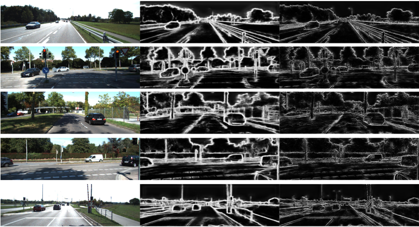
Figure 5: Qualitative demonstrations of better edge predictions after multi-task learning. From left: image in the KITTI 2015 training set, edge map from the Multicue-pretrained edge detection sub-network, edge map from EdgeStereo after multi-task learning. Non-maximum suppression (NMS) is not adopted to thin detected edges.

Table 6: Quantitative demonstrations of better disparity estimates near boundaries after incorporating edge cues. Experiments are conducted on the KITTI validation sets.

Model	KITTI 2012 val		KITTI 2015 val
	$>3\,px$	EPE	$>3\,px$	EPE
Baseline model (without edge cues)	3.957	0.764	4.354	0.989
EdgeStereo	3.401	0.704	3.968	0.946

Table 7: Comparison with other stereo matching methods on the FlyingThings3D test set.

Metric		SGMhirschmuller2005accurate	MC-CNNzbontar2016stereo	DispNetmayer2016large	CRLpang2017cascade	GC-Netkendall2017end	PSMNetchang2018pyramid	iResNetliang2017learning	SegStereoyang_segstereo	Baseline	EdgeStereo
Protocol 1	$>3\,px$	12.54	13.70	9.67	6.37	8.13	4.69	4.58	4.61	4.72	4.30
	EPE	4.50	3.79	1.84	1.33	2.83	1.65	1.05	1.36	1.32	1.27
Protocol 2	$>3\,px$	-	-	9.31	5.97	7.73	4.14	4.40	4.27	4.40	3.96
	EPE	-	-	1.70	1.21	2.15	0.98	0.95	0.91	0.82	0.74

Table 8: Comparison with other stereo matching methods in “Reflective Regions” on the KITTI stereo 2012 benchmark (March 5, 2019).

Metric	SGMhirschmuller2005accurate	MC-CNNzbontar2016stereo	DispNetmayer2016large	GC-Netkendall2017end	Displetsguney2015displets	PSMNetchang2018pyramid	iResNetliang2017learning	PDSNettulyakov2018practical	SegStereoyang_segstereo	Baseline	EdgeStereo
$>3\,px$	27.39	17.09	16.04	10.80	8.40	8.36	7.40	6.50	6.35	8.53	5.84
EPE	5.1 px	3.2 px	2.1 px	1.8 px	1.9 px	1.4 px	1.2 px	1.4 px	1.1 px	1.5 px	1.0 px

4.4.1 Stereo Matching Helps Edge Detection

EdgeStereo_RP_4 is adopted for verification. We first train the edge branch on Multicue, then fix it and train the disparity branch on FlyingThings3D, finally train two branches simultaneously on FlyingThings3D. We compare the Multicue-pretrained edge detection sub-network with the edge branch in EdgeStereo after multi-task learning.

Firstly we give quantitative demonstrations on the BSDS500 edge detection dataset. As shown in Table 5, ODS F-measures and OIS F-measures on the BSDS500 training, validation and test sets are all improved after multi-task learning, even though the BSDS500 dataset is not used for pretraining and the FlyingThings3D training set does not contain ground-truth edge annotations during training.

Next we give qualitative demonstrations on the KITTI stereo 2015 training set without edge annotations. As shown in Fig. 5, after multi-task learning, edge predictions are significantly refined and details are highlighted in the produced edge maps, even though the model is not trained on KITTI 2015. Hence the mutual exploitation of stereo and edge information under the guidance of the edge-aware smoothness loss is beneficial for edge detection task, proving the effectiveness of the multi-task learning in our unified model.

4.4.2 Edge Detection Helps Stereo Matching

Several qualitative and quantitative demonstrations are already provided in Fig. 1 and Table 1. We further prove that disparity estimates near boundaries are more accurate after incorporating edge cues. Considering edge annotations are not provided in the KITTI stereo datasets, we treat the edge predictions from the FlyingThings3D-pretrained EdgeStereo model as boundaries for evaluation. As shown in Table 6, after incorporating edge cues, $3$-pixel errors near boundaries are reduced by $14.1\%$ and $8.7\%$ on the KITTI 2012 and 2015 validation sets respectively, compared with the baseline model.

Table 9: Comparison with other stereo matching methods on the KITTI stereo 2012 benchmark (March 1, 2019).

	$>\,2$px		$>\,3$px		$>\,4$px		$>\,5$px		EPE
	Noc	All	Noc	All	Noc	All	Noc	All	Noc
PSMNet chang2018pyramid	2.44	3.01	1.49	1.89	1.12	1.42	0.90	1.15	0.5 px
SegStereoyang_segstereo	2.66	3.19	1.68	2.03	1.25	1.52	1.00	1.21	0.5 px
iResNet liang2017learning	2.69	3.34	1.71	2.16	1.30	1.63	1.06	1.32	0.5 px
GC-Net kendall2017end	2.71	3.46	1.77	2.30	1.36	1.77	1.12	1.46	0.6 px
PDSNet tulyakov2018practical	3.82	4.64	1.92	2.53	1.38	1.85	1.12	1.51	0.9 px
L-ResMatch shaked2016improved	3.64	5.06	2.27	3.40	1.76	2.67	1.50	2.26	0.7 px
SGM-Net seki2017sgm	3.60	5.15	2.29	3.50	1.83	2.80	1.60	2.36	0.7 px
Displets guney2015displets	3.90	4.92	2.37	3.09	1.97	2.52	1.72	2.17	0.7 px
MC-CNN zbontar2016stereo	3.90	5.45	2.43	3.63	1.90	2.85	1.64	2.39	0.7 px
DispNet mayer2016large	7.38	8.11	4.11	4.65	2.77	3.20	2.05	2.39	0.9 px
SGM hirschmuller2005accurate	8.66	10.16	5.76	7.00	4.38	5.41	3.56	4.41	1.2 px
Baseline	2.91	3.55	1.81	2.27	1.29	1.61	1.07	1.25	0.5 px
EdgeStereo	2.32	2.88	1.46	1.83	1.07	1.34	0.83	1.04	0.4 px

Table 10: Comparison with other stereo matching methods on the KITTI stereo 2015 benchmark (March 1, 2019).

	All Pixels			Non-Occluded Pixels			Runtime
	D1-bg	D1-fg	D1-all	D1-bg	D1-fg	D1-all	(s)
SegStereoyang_segstereo	1.88	4.07	2.25	1.76	3.70	2.08	0.6
PSMNet chang2018pyramid	1.86	4.62	2.32	1.71	4.31	2.14	0.41
iResNet liang2017learning	2.25	3.40	2.44	2.07	2.76	2.19	0.12
PDSNet tulyakov2018practical	2.29	4.05	2.58	2.09	3.68	2.36	0.5
CRL pang2017cascade	2.48	3.59	2.67	2.32	3.12	2.45	0.47
GC-Net kendall2017end	2.21	6.16	2.87	2.02	5.58	2.61	0.9
LRCR jie2018left	2.55	5.42	3.03	2.23	4.19	2.55	49.2
DRR gidaris2016detect	2.58	6.04	3.16	2.34	4.87	2.76	0.4
L-ResMatch shaked2016improved	2.72	6.95	3.42	2.35	5.74	2.91	48
Displets guney2015displets	3.00	5.56	3.43	2.73	4.95	3.09	265
SGM-Net seki2017sgm	2.66	8.64	3.66	2.23	7.44	3.09	67
MC-CNN zbontar2016stereo	2.89	8.88	3.88	2.48	7.64	3.33	67
DispNet mayer2016large	4.32	4.41	4.34	4.11	3.72	4.05	0.06
SGM hirschmuller2005accurate	5.06	13.00	6.38	4.43	11.68	5.62	0.11
Baseline	2.11	3.99	2.41	1.94	3.35	2.17	0.26
EdgeStereo	1.84	3.30	2.08	1.69	2.94	1.89	0.32

Table 11: Comparison with other stereo matching methods on the Middlebury benchmark (July 29, 2019).

	MC-CNN-fstzbontar2016stereo (Half)	SGMhirschmuller2005accurate (Half)	iResNetliang2017learning (Half)	PSMNet_ROBchang2018pyramid (Quarter)	EdgeStereo (Full)
$2$-pixel error	9.47%	18.4%	22.9%	42.1%	18.7%

4.5 Comparison with Other Stereo Matching Methods

EdgeStereo_RP_4 is adopted as the final EdgeStereo model, with three outputs for training. Through experiments, the loss weights $\lambda_{r}^{2},\lambda_{r}^{1},\lambda_{r}^{0}$ for the disparity regression loss are set to $0.6,0.8,1.0$; the loss weights $\lambda_{sm}^{2},\lambda_{sm}^{1},\lambda_{sm}^{0}$ for the edge-aware smoothness loss are set to $0.06,0.08,0.1$.

4.5.1 FlyingThings3D Results

We first compare EdgeStereo with several non-end-to-end stereo matching methods, including SGM hirschmuller2005accurate , MC-CNN zbontar2016stereo and DRR gidaris2016detect . Next we compare EdgeStereo with the state-of-the-art end-to-end stereo matching networks, including DispNetC mayer2016large , CRL pang2017cascade , GC-Net kendall2017end , PSMNet chang2018pyramid , iResNet liang2017learning and SegStereo yang_segstereo . For comparison, we use models made available by authors except GC-Net, while we retrain GC-Net following the settings in their paper. As can be seen in Table 7, EdgeStereo achieves the best performance under two testing protocols.

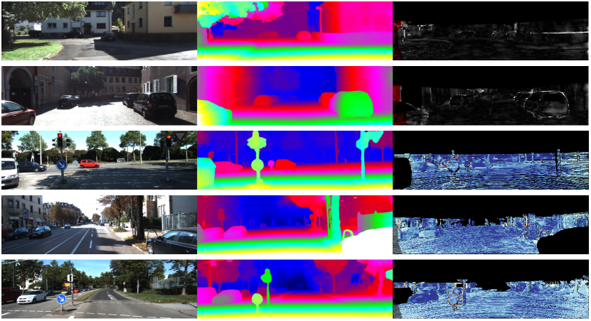
Figure 6: Qualitative results on the KITTI 2012 and 2015 test sets. From left: left stereo image, disparity estimates, error map.

Table 12: The generalization performance of state-of-the-art end-to-end stereo matching methods. To compare generalization capability, FlyingThings3D-pretrained models are evaluated on the KITTI 2012 and 2015 training sets, collaborative-pretrained (FlyingThings3D plus CityScapes) models are evaluated on the KITTI 2012 and Middlebury 2014 training sets.

Dataset and Metric		DispNet	CRL	iResNet	PSMNet	SegStereo	Baseline	EdgeStereo
1. FlyingThings3D Pretrain
KITTI 2012 training	$>3\,px$	12.542	9.073	7.895	27.333	12.808	16.783	12.274
	EPE	1.753	1.387	1.278	5.549	2.052	3.333	1.963
KITTI 2015 training	$>3\,px$	12.881	8.885	7.424	29.868	11.234	16.179	12.467
	EPE	1.596	1.357	1.213	6.445	2.187	3.653	2.068
2. FlyingThings3D + CityScapes Pretrain
KITTI 2012 training	$>3\,px$	6.373	5.705	4.867	5.716	5.476	5.677	5.239
	EPE	1.194	1.096	1.001	1.137	1.113	1.010	0.999
Middlebury (Half)	$>3\,px$	15.684	10.987	10.475	13.859	14.477	13.120	11.136
	EPE	2.217	1.676	1.583	1.987	2.173	2.109	1.552

4.5.2 KITTI 2012 Results

EdgeStereo is finetuned using all $194$ training pairs, then the testing results are submitted to the KITTI 2012 online leaderboard. For evaluation, we use the percentage of erroneous pixels ($>2px$, $>3px$, $>4px$, $>5px$) and EPE in non-occluded (Noc) and all (All) regions. The results are shown in Table 9. As can be seen, by the time of the paper submission, EdgeStereo outperforms all published stereo matching methods in all evaluation metrics. We also finetune the baseline model on the KITTI 2012 training set, then submit corresponding results to the benchmark. By leveraging edge cues, EdgeStereo is obviously superior to the baseline model, producing more reliable disparity estimates in detailed structures, large occlusions and near boundaries.

We also compare EdgeStereo with state-of-the-art stereo methods in “Reflective Regions” on the KITTI stereo 2012 benchmark. As shown in Table 8, EdgeStereo surpasses the baseline model and other methods by a noteworthy margin, especially the SegStereo yang_segstereo which utilizes foreground semantic information, and the Displets guney2015displets which resolves stereo ambiguities using object knowledge. Hence incorporating semantic-meaningful edge information can provide beneficial geometric knowledge for finding correspondences in texture-less regions.

4.5.3 KITTI 2015 Results

We also submit the testing results to the KITTI 2015 online leaderboard. For evaluation, we use the $3$-pixel error of background (D1-bg), foreground (D1-fg) and all pixels (D1-all) in non-occluded and all regions. The results are shown in Table 10. As can be seen, EdgeStereo achieves the best performance compared with the baseline model and all published stereo matching methods, meanwhile it is more efficient than the 3-D convolutional neural networks and cascaded structures. Fig. 6 gives qualitative results on the KITTI test sets.

4.5.4 Middlebury 2014 Results

On the validation set (half size), the baseline model without edge cues achieves a a $2$-pixel error of $12.473\%$ and an EPE of $1.225$, while EdgeStereo achieves a $2$-pixel error of $11.540\%$ and an EPE of $1.139$, demonstrating the effectiveness of incorporating edge cues for disparity learning.

Next we compare EdgeStereo with other methods on the benchmark. Since the Middlebury dataset is too small, among published end-to-end stereo networks, only iResNet and PSMNet (ROB) report their results on this tiny dataset. As can be seen from Table 11, EdgeStereo outperforms iResNet and PSMNet by a noteworthy margin. However it performs worse than the non-end-to-end method MC-CNN. On the Middlebury benchmark, the top-performing methods are non-end-to-end networks and some sophisticated hand engineered methods rather than end-to-end stereo networks. For non-end-to-end networks, training is conducted based on pairs of image patches and the Middlebury training set can provide sufficient training samples, hence their training processes are much more complete than end-to-end networks. The proposed EdgeStereo is an end-to-end architecture with a large capacity of feature representation and context characterization. Even if powerful data augmentations are used during training, the Middlebury training set is too small to fit the capacity of EdgeStereo. Hence we argue that the powerfulness of EdgeStereo should be better evaluated on datasets with larger scales.

4.6 Generalization Performance

4.6.1 Cross-domain Experiments

The generalization capability of an end-to-end disparity estimation network is important, since obtaining ground-truth disparities using LiDAR is costly, and most real-world stereo datasets are not large enough to train a model without over-fitting. FlyingThings3D pretraining and collaborative pretraining yang2018srcdisp (FlyingThings3D plus CityScapes) are the most effective pretraining methods for end-to-end stereo networks, which are adopted to compare the generalization performance of state-of-the-art stereo matching methods. Firstly, we compare FlyingThings3D pretrained models on the KITTI 2012 and 2015 training sets. We use publicly available models (provided by authors) of DispNet, CRL, SegStereo and PSMNet for comparison and train iResNet on Flyingthings3D. Secondly, we compare collaboratively pretrained (FlyingThings3D plus CityScapes) models on the KITTI 2012 and Middlebury 2014 training sets. Since the collaborative pretraining scheme is not used in the previously published methods, we pretrain all competitors (DispNet, CRL, SegStereo, iResNet and PSMNet) following the same scheduling reported in the original papers.

The results are shown in Table 12. As can be seen, Flyingthings3D pretrained EdgeStereo model achieves comparable generalization performance with DispNet and SegStereo, meanwhile being significantly better than 3-D convolutional networks (PSMNet). However, Flyingthings3D pretrained EdgeStereo preforms slightly worse than CRL and iResNet on KITTI training sets, since the capacity of our EdgeStereo is much larger than CRL and iResNet, while the synthetic Flyingthings3D dataset has a quite different domain with real-world KITTI datasets (e.g. unreasonably large disparities) that EdgeStereo has learnt to adapt. When comparing collaboratively pretrained models, where the real-world Cityscapes dataset is used for pretraining, EdgeStereo achieves comparable generalization performance with iResNet. In addition, EdgeStereo outperforms all other competitors on the Middlebury benchmark, KITTI benchmarks and Flyingthings3D test set, demonstrating the capability of our EdgeStereo on different domains. Collaboratively pretrained EdgeStereo achieves a $3$-pixel error of $5.239\%$ on the KITTI 2012 training set, which is a promising result for practical use when obtaining dense ground-truth disparities is costly. In addition, when pretrained and evaluated on datasets with different domains, EdgeStereo outperforms the baseline model obviously after incorporating edge cues for multi-task learning.

Figure 7: Disparity estimations of the collaboratively pretrained EdgeStereo on the self-built Middlebury validation set (indoor edgeless scenarios).

Table 13: Comparison between the collaboratively pretrained EdgeStereo and baseline on the self-built Middlebury validation set (indoor edgeless scenarios).

	$3$-pixel error	EPE
Baseline	2.742	0.622
EdgeStereo	2.252	0.570

Table 14: Comparison between our new work and the previous version song2018stereo .

	KITTI2012 test	KITTI2012 reflective regions	KITTI2015 test	Flyingthings3D
Previous song2018stereo	1.73%	7.01%	2.59%	4.70%/0.99
New	1.46%	5.84%	2.08%	3.96%/0.74

4.6.2 Performance in Indoor Edgeless Scenarios

To further demonstrate that our proposed method also works well in edgeless indoor scenarios, firstly we choose $10$ edgeless stereo pairs from the Middlebury training set as a validation set, next we compare the collaboratively pretrained (FlyingThings3D plus CityScapes) EdgeStereo model and baseline model (without the edge detection branch) on this validation set.

As can be seen from Table 13, the EdgeStereo model achieves a satisfactory $3$-pixel error of $2.252\%$ on this challenging full-resolution Middlebury validation set, even if the model is pretrained using unrealistic data (Flyingthings3D) and outdoor data (Cityscapes). In addition, EdgeStereo outperforms the baseline model on these edgeless scenarios after multi-task learning, demonstrating that the proposed model would not suffer from the edge branch in these scenarios. The qualitative demonstrations are given in Fig. 7. As can be seen, the collaboratively pretrained EdgeStereo produces consistent disparity estimations in edgeless scenarios.

4.7 Comparison with the Previous Version

Compared with our ACCV version song2018stereo : (1) We change the backbone from the ImageNet pretrained VGG16 to a more powerful feature extractor ResNet50, and we also change the encoder structure to a ResNet-like structure for better intermediate representations; (2) We re-design the structure of the residual pyramid and make it more effective, where multi-scale features are used for binocular warping and cost volume generation; (3) We refine multi-task learning mechanism, where the edge-aware smoothness loss is enabled to be propagated back to the disparity branch and edge branch simultaneously, then both the disparity map and edge map can be optimized under the guidance of the edge-aware smoothness loss. Consequently we obtain the most important conclusion in this paper: edge detection and stereo matching can help each other based on our unified model.

In conclusion, we re-design the overall architecture where all modules are proved to be more effective. Finally, we will give some quantitative comparisons in Table 14. As can be seen, the new architecture outperforms the original one on all test sets and the challenging reflective regions.

5 Conclusion and Future Work

In this paper, we propose an effective multi-task learning network EdgeStereo for stereo matching and edge detection. To effectively incorporate edge cues into the disparity estimation pipeline for multi-task learning, we design the edge feature embedding and propose the edge-aware smoothness loss. The experimental results show that the disparity estimates in texture-less regions, large occlusions, detailed structures and near boundaries are significantly improved after incorporating edge cues. Correspondingly, our EdgeStereo achieves the best performance on the FlyingThings3D dataset, meanwhile outperforming other published stereo matching methods on the KITTI stereo 2012 and 2015 benchmarks. EdgeStereo also ranks the first on the online leaderboard of the KITTI 2012 “Reflective Regions” evaluation. In addition, we provide both qualitative and quantitative demonstrations that edge predictions are improved after multi-task learning, even if ground-truth edge annotations are not provided for training. Finally we prove that EdgeStereo has a comparable generalization capability for disparity estimation. In conclusion, stereo matching task and edge detection task can promote each other through the geometric knowledge learned from the multi-task interactions in EdgeStereo.

In future work, we intend to apply the multi-task learning mechanism of EdgeStereo to other dense matching applications, such as optical flow and multi-view reconstruction etc. In addition, we consider to explicitly model geometric constraints from stereo matching for edge detection to further improve the quality of edge predictions. Finally, we consider to incorporate more tasks, such as semantic segmentation and instance segmentation etc, into our unified model. It will be a future direction to achieve an integrated vision system with a clear and interpretable architecture.

- (1) Arbelaez, P., Maire, M., Fowlkes, C., Malik, J.: Contour detection and hierarchical image segmentation. TPAMI 33(5), 898–916 (2011)
- (2) Barron, J.T.: A more general robust loss function. arXiv preprint arXiv:1701.03077 (2017)
- (3) Barron, J.T., Adams, A., Shih, Y., Hernández, C.: Fast bilateral-space stereo for synthetic defocus. In: CVPR, pp. 4466–4474 (2015)
- (4) Canny, J.: A computational approach to edge detection. TPAMI (6), 679–698 (1986)
- (5) Chang, J.R., Chen, Y.S.: Pyramid stereo matching network. In: CVPR (2018)
- (6) Chen, Z., Sun, X., Wang, L., Yu, Y., Huang, C.: A deep visual correspondence embedding model for stereo matching costs. In: ICCV, pp. 972–980 (2015)
- (7) Cheng, J., Tsai, Y.H., Wang, S., Yang, M.H.: SegFlow: Joint learning for video object segmentation and optical flow. In: ICCV, pp. 686–695 (2017)
- (8) Cordts, M., Omran, M., Ramos, S., Rehfeld, T., Enzweiler, M., Benenson, R., Franke, U., Roth, S., Schiele, B.: The cityscapes dataset for semantic urban scene understanding. In: CVPR, pp. 3213–3223 (2016)
- (9) Deng, J., Dong, W., Socher, R., Li, L.J., Li, K., Fei-Fei, L.: Imagenet: A large-scale hierarchical image database. In: CVPR, pp. 248–255 (2009)
- (10) Dollar, P., Tu, Z., Belongie, S.: Supervised learning of edges and object boundaries. In: CVPR, vol. 2, pp. 1964–1971 (2006)
- (11) Dollár, P., Zitnick, C.L.: Fast edge detection using structured forests. TPAMI 37(8), 1558–1570 (2015)
- (12) Dosovitskiy, A., Fischery, P., Ilg, E., HUsser, P.: Flownet: Learning optical flow with convolutional networks. In: ICCV, pp. 2758–2766 (2015)
- (13) Garg, R., BG, V.K., Carneiro, G., Reid, I.: Unsupervised cnn for single view depth estimation: Geometry to the rescue. In: ECCV, pp. 740–756 (2016)
- (14) Geiger, A., Lenz, P., Urtasun, R.: Are we ready for autonomous driving? the kitti vision benchmark suite. In: CVPR, pp. 3354–3361 (2012)
- (15) Geiger, A., Roser, M., Urtasun, R.: Efficient large-scale stereo matching. In: ACCV, pp. 25–38 (2010)
- (16) Gidaris, S., Komodakis, N.: Detect, replace, refine: Deep structured prediction for pixel wise labeling. In: CVPR, pp. 5248–5257 (2017)
- (17) Godard, C., Aodha, O.M., Brostow, G.J.: Unsupervised monocular depth estimation with left-right consistency. In: CVPR, pp. 6602–6611 (2017)
- (18) Godard, C., Mac Aodha, O., Brostow, G.J.: Unsupervised monocular depth estimation with left-right consistency. In: CVPR (2017)
- (19) Guney, F., Geiger, A.: Displets: Resolving stereo ambiguities using object knowledge. In: CVPR, pp. 4165–4175 (2015)
- (20) He, K., Zhang, X., Ren, S., Sun, J.: Deep residual learning for image recognition. In: CVPR, pp. 770–778 (2016)
- (21) Heise, P., Jensen, B., Klose, S., Knoll, A.: Fast dense stereo correspondences by binary locality sensitive hashing. In: ICRA, pp. 105–110 (2015)
- (22) Hirschmuller, H.: Accurate and efficient stereo processing by semi-global matching and mutual information. In: CVPR, pp. 807–814 (2005)
- (23) Jia, Y., Shelhamer, E., Donahue, J., Karayev, S., Long, J., Girshick, R., Guadarrama, S., Darrell, T.: Caffe: Convolutional architecture for fast feature embedding. In: ACMMM, pp. 675–678 (2014)
- (24) Jie, Z., Wang, P., Ling, Y., Zhao, B., Wei, Y., Feng, J., Liu, W.: Left-right comparative recurrent model for stereo matching. In: CVPR, pp. 3838–3846 (2018)
- (25) Kendall, A., Gal, Y., Cipolla, R.: Multi-task learning using uncertainty to weigh losses for scene geometry and semantics. In: Proceedings of the IEEE Conference on Computer Vision and Pattern Recognition, pp. 7482–7491 (2018)
- (26) Kendall, A., Martirosyan, H., Dasgupta, S., Henry, P., Kennedy, R.: End-to-end learning of geometry and context for deep stereo regression. In: ICCV (2017)
- (27) Klaus, A., Sormann, M., Karner, K.: Segment-based stereo matching using belief propagation and a self-adapting dissimilarity measure. In: ICPR, vol. 3, pp. 15–18 (2006)
- (28) Knobelreiter, P., Reinbacher, C., Shekhovtsov, A., Pock, T.: End-to-end training of hybrid cnn-crf models for stereo. In: CVPR, pp. 2339–2348 (2017)
- (29) Kolmogorov, V., Zabih, R.: Computing visual correspondence with occlusions using graph cuts. In: ICCV, vol. 2, pp. 508–515 (2001)
- (30) Kuznietsov, Y., Stuckler, J., Leibe, B.: Semi-supervised deep learning for monocular depth map prediction. In: CVPR, pp. 6647–6655 (2017)
- (31) Liang, Z., Feng, Y., Guo, Y., Liu, H.: Learning deep correspondence through prior and posterior feature constancy. In: CVPR (2018)
- (32) Liu, Y., Cheng, M.M., Hu, X., Wang, K., Bai, X.: Richer convolutional features for edge detection. In: CVPR, pp. 5872–5881 (2017)
- (33) Liu, Y., Lew, M.S.: Learning relaxed deep supervision for better edge detection. In: CVPR, pp. 231–240 (2016)
- (34) Long, J., Shelhamer, E., Darrell, T.: Fully convolutional networks for semantic segmentation. In: CVPR, pp. 3431–3440 (2015)
- (35) Lu, C., Uchiyama, H., Thomas, D., Shimada, A., Taniguchi, R.i.: Sparse cost volume for efficient stereo matching. Remote Sensing 10(11), 1844 (2018)
- (36) Luo, W., Schwing, A.G., Urtasun, R.: Efficient deep learning for stereo matching. In: CVPR, pp. 5695–5703 (2016)
- (37) Mao, J., Xiao, T.: What can help pedestrian detection? In: CVPR (2017)
- (38) Mayer, N., Ilg, E., Hausser, P., Fischer, P., Cremers, D., Dosovitskiy, A., Brox, T.: A large dataset to train convolutional networks for disparity, optical flow, and scene flow estimation. In: CVPR, pp. 4040–4048 (2016)
- (39) Mei, X., Sun, X., Zhou, M., Jiao, S., Wang, H., Zhang, X.: On building an accurate stereo matching system on graphics hardware. In: ICCVW, pp. 467–474 (2011)
- (40) Mély, D.A., Kim, J., McGill, M., Guo, Y., Serre, T.: A systematic comparison between visual cues for boundary detection. Vision research 120, 93–107 (2016)
- (41) Menze, M., Geiger, A.: Object scene flow for autonomous vehicles. In: CVPR, pp. 3061–3070 (2015)
- (42) Mottaghi, R., Chen, X., Liu, X., Cho, N.G., Lee, S.W.: The role of context for object detection and semantic segmentation in the wild. In: CVPR, pp. 891–898 (2014)
- (43) Nam, K.W., Park, J., Kim, I.Y., Kim, K.G.: Application of stereo-imaging technology to medical field. Healthcare informatics research 18(3), 158–163 (2012)
- (44) Pang, J., Sun, W., Ren, J., Yang, C., Yan, Q.: Cascade residual learning: A two-stage convolutional neural network for stereo matching. In: ICCV Workshop, vol. 3, pp. 1057–7149 (2017)
- (45) Ramirez, P.Z., Poggi, M., Tosi, F., Mattoccia, S., Di Stefano, L.: Geometry meets semantics for semi-supervised monocular depth estimation. In: ACCV, pp. 298–313 (2018)
- (46) Ronneberger, O., Fischer, P., Brox, T.: U-net: Convolutional networks for biomedical image segmentation. In: MICCAI, pp. 234–241 (2015)
- (47) Scharstein, D., Hirschmüller, H., Kitajima, Y., Krathwohl, G., Nešić, N., Wang, X., Westling, P.: High-resolution stereo datasets with subpixel-accurate ground truth. In: GCPR, pp. 31–42 (2014)
- (48) Scharstein, D., Szeliski, R.: A taxonomy and evaluation of dense two-frame stereo correspondence algorithms. IJCV 47(1-3), 7–42 (2002)
- (49) Schmid, K., Tomic, T., Ruess, F., Hirschmüller, H., Suppa, M.: Stereo vision based indoor/outdoor navigation for flying robots. In: IROS, pp. 3955–3962 (2013)
- (50) Seki, A., Pollefeys, M.: SGM-Nets: Semi-global matching with neural networks. In: CVPR, pp. 21–26 (2017)
- (51) Shaked, A., Wolf, L.: Improved stereo matching with constant highway networks and reflective confidence learning. In: CVPR, pp. 4641–4650 (2017)
- (52) Shean, D.E., Alexandrov, O., Moratto, Z.M., Smith, B.E., Joughin, I.R., Porter, C., Morin, P.: An automated, open-source pipeline for mass production of digital elevation models (dems) from very-high-resolution commercial stereo satellite imagery. ISPRS (2016)
- (53) Song, X., Zhao, X., Hu, H., Fang, L.: Edgestereo: A context integrated residual pyramid network for stereo matching. In: ACCV (2018)
- (54) Sun, D., Yang, X., Liu, M.Y., Kautz, J.: Pwc-net: Cnns for optical flow using pyramid, warping, and cost volume. In: CVPR, pp. 8934–8943 (2018)
- (55) Tonioni, A., Poggi, M., Mattoccia, S., Di Stefano, L.: Unsupervised adaptation for deep stereo. In: ICCV, pp. 1605–1613 (2017)
- (56) Tonioni, A., Tosi, F., Poggi, M., Mattoccia, S., Stefano, L.D.: Real-time self-adaptive deep stereo. In: CVPR, pp. 195–204 (2019)
- (57) Tulyakov, S., Ivanov, A., Fleuret, F.: Practical deep stereo (pds): Toward applications-friendly deep stereo matching. In: NIPS (2018)
- (58) Xie, S., Tu, Z.: Holistically-nested edge detection. In: ICCV, pp. 1395–1403 (2015)
- (59) Yang, G., Deng, Z., Lu, H., Li, Z.: Src-disp: Synthetic-realistic collaborative disparity learning for stereo mathcing. In: ACCV (2018)
- (60) Yang, G., Zhao, H., Shi, J., Deng, Z., Jia, J.: Segstereo: Exploiting semantic information for disparity estimation. In: ECCV (2018)
- (61) Yu, L., Wang, Y., Wu, Y., Jia, Y.: Deep stereo matching with explicit cost aggregation sub-architecture. In: AAAI (2018)
- (62) Zagoruyko, S., Komodakis, N.: Learning to compare image patches via convolutional neural networks. In: CVPR, pp. 4353–4361 (2015)
- (63) Zbontar, J., LeCun, Y.: Computing the stereo matching cost with a convolutional neural network. In: CVPR, pp. 1592–1599 (2015)
- (64) Zbontar, J., LeCun, Y.: Stereo matching by training a convolutional neural network to compare image patches. JMLR 17(1-32), 2 (2016)
- (65) Zhang, L., Seitz, S.M.: Estimating optimal parameters for mrf stereo from a single image pair. TPAMI 29(2), 331–342 (2007)
- (66) Zhao, H., Shi, J., Qi, X., Wang, X., Jia, J.: Pyramid scene parsing network. In: CVPR, pp. 2881–2890 (2017)
- (67) Zhong, Y., Dai, Y., Li, H.: Self-supervised learning for stereo matching with self-improving ability. In: CVPR (2017)
- (68) Zhou, C., Zhang, H., Shen, X., Jia, J.: Unsupervised learning of stereo matching. In: ICCV, vol. 2 (2017)