Domain Adaptation with Asymmetrically-Relaxed Distribution Alignment

Abstract

Domain adaptation addresses the common problem when the target distribution generating our test data drifts from the source (training) distribution. While absent assumptions, domain adaptation is impossible, strict conditions, e.g. covariate or label shift, enable principled algorithms. Recently-proposed domain-adversarial approaches consist of aligning source and target encodings, often motivating this approach as minimizing two (of three) terms in a theoretical bound on target error. Unfortunately, this minimization can cause arbitrary increases in the third term, e.g. they can break down under shifting label distributions. We propose asymmetrically-relaxed distribution alignment, a new approach that overcomes some limitations of standard domain-adversarial algorithms. Moreover, we characterize precise assumptions under which our algorithm is theoretically principled and demonstrate empirical benefits on both synthetic and real datasets.

1 Introduction

Despite breakthroughs in supervised deep learning across a variety of challenging tasks, current techniques depend precariously on the i.i.d. assumption. Unfortunately, real-world settings often demand not just generalization to unseen examples but robustness under a variety of shocks to the data distribution. Ideally, our models would leverage unlabeled test data, adapting in real time to produce improved predictions. Unsupervised domain adaptation formalizes this problem as learning a classifier from labeled source domain data and unlabeled data from a target domain, to maximize performance on the target distribution.

Without further assumptions, guarantees of target-domain accuracy are impossible (Ben-David et al., 2010b). However, well-chosen assumptions can make possible algorithms with non-vacuous performance guarantees. For example, under the covariate shift assumption (Heckman, 1977; Shimodaira, 2000), although the input marginals can vary between source and target ($p_{S}(x)\neq p_{T}(x)$), the conditional distribution of the labels (given features) exhibits invariance across domains ($p_{S}(y|x)=p_{T}(y|x)$). Some consider the reverse setting label shift (Saerens et al., 2002; Zhang et al., 2013; Lipton et al., 2018), where although the label distribution shifts ($p_{S}(y)\neq p_{T}(y)$), the class-conditional input distribution is invariant ($p_{S}(x|y)=p_{T}(x|y)$). Traditional approaches to both problems require the source distributions’ support to cover the target support, estimating adapted classifiers via importance-weighted risk minimization (Shimodaira, 2000; Huang et al., 2007; Gretton et al., 2009; Yu & Szepesvári, 2012; Lipton et al., 2018).

Problematically, assumptions of contained support are violated in practice. Moreover, most theoretical analyses do not guaranteed target accuracy when the source distribution support does not cover that of the target. A notable exception, Ben-David et al. (2010a) leverages capacity constraints on the hypothesis class to enable generalization to out-of-support samples. However, their results (i) do not hold for high-capacity hypothesis classes, e.g., neural networks; and (ii) do not provide intuitive interpretations on what is sufficient to guarantee a good target domain performance.

A recent sequence of deep learning papers have proposed empirically-justified adversarial training schemes aimed at practical problems with non-overlapping supports (Ganin et al., 2016; Tzeng et al., ). Example problems include generalizing from gray-scale images to colored images or product images on white backgrounds to photos of products in natural settings. While importance-weighting solutions are useless here (with non-overlapping support, weights are unbounded), domain-adversarial networks (Ganin et al., 2016) and subsequently-proposed variants report strong empirical results on a variety of image recognition challenges.

The key idea of domain-adversarial networks is to simultaneously minimize the source error and align the two distributions in representation space. The scheme consists of an encoder, a label classifier, and a domain classifier. During training, the domain classifier is optimized to predict each image’s domain given its encoding. The label classifier is optimized to predict labels from encodings (for source images). The encoder weights are optimized for the twin objectives of accurate label classification (of source data) and fooling the domain classifier (for all data).

Although Ganin et al. (2016) motivate their idea via theoretical results due to Ben-David et al. (2010a), the theory is insufficient to justify their method. Put simply, Ben-David et al. (2010a) bound the test error by a sum of three terms. The domain-adversarial objective minimizes two among these, but this minimization may cause the third term to increase. This is guaranteed to happen when the label distribution shifts between source and target. Consider the case of cat-dog classification with non-overlapping support. Say that the source distribution contains $50\%$ dogs and $50\%$ cats, while the target distribution contains $25\%$ dogs and $75\%$ cats. Successfully aligning these distributions in representation space requires the classifier to predict the same fraction of dogs and cats on source and target. If one achieves $100\%$ accuracy on the source data, then target accuracy will be at most $75\%$ (Figure 1(a)).

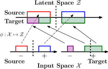
(a) Exact matching

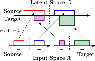
(b) Relaxed matching

Figure 1: (a) In order to match the latent space distributions exactly, a model must map some elements of positive class in the target domain to some elements of negative class in the source domain. (b) A better mapping is achieved by requiring only that the source covers the target in the latent space.

In this paper, we propose asymmetrically-relaxed distribution alignment, a relaxed distance for aligning data across domains that can be minimized without requiring latent-space distributions to match exactly. The new distance is minimized whenever the density ratios in representation space from target to source are upper bounded by a certain constant, such that the target representation support is contained in the source representation’s. The relaxed distribution alignment need not lead to a poor classifier on the target domain under label distribution mismatch (Figure 1(b)). We demonstrate theoretically that the relaxed alignment is sufficient for a good target domain performance under a concrete set of assumptions on the data distributions. Further, we propose several practical ways to achieve the relaxed distribution alignment, translating the new distance into adversarial learning objectives. Empirical results on synthetic and real datasets show that incorporating our relaxed distribution alignment loss into adversarial domain adaptation gives better classification performance on the target domain. We make the following key contributions:

• We propose an asymmetrically relaxed distribution matching objective, overcoming the limitation of standard objectives under label distribution shift.

• We provide theoretical analysis demonstrating that under a clear set of assumptions, the asymmetrically relaxed distribution alignment can provide target-domain performance guarantees.

• We propose several distances that satisfy the desired properties and are optimizable by adversarial training.

• We empirically show that our asymmetrically relaxed distribution matching losses improve target performance when there is a label distribution shift in the target domain, and perform comparably otherwise.

2 Preliminaries

We use subscripts $S$ and $T$ to distinguish between source and target domains, e.g., $p_{S}$ and $p_{T}$, and employ the notation $U$ for statements that are true for any domain $U\in\{S,T\}$. For simplicity, we dispense with some rigorousness in notating probability measures. For example, we use the terms measure and distribution interchangeably and assume that a density function exists when necessary without explicitly stating the base measure and required regularity conditions. We use a single lowercase letter, e.g. $p$, to denote both the probability measure function and the probability density function: $p(x)$ is a density when the input $x$ is a single point while $p(C)$ is a probability when the input $C$ is a set. We will use $\mathrm{Supp}(p)$ to denote the support of distribution $p$, i.e., the set of points where the density is positive. Similarly, for a function mapping $\phi$, $\phi(x)$ denotes an output if $x$ is a point and $\phi(C)$ denotes the image if $C$ is a set. The inverse mapping $\phi^{-1}$ always outputs a set (the inverse image) regardless of whether its input is a point or a set. We will also be less careful about the use of $\sup$ v.s. $\max$, $\inf$ v.s. $\min$ and “everywhere” v.s. “almost everywhere”. $\mathbbm{1}\left\{\cdot\right\}$ is used as the indicator function for statements that output $1$ if the statement is true and $0$ otherwise. For two functions $f$ and $g$ we use $f\equiv g$ to denote that $f(x)=g(x)$ for every input $x$.

Unsupervised domain adaptation

For simplicity, we address the binary classification scenario. Let $\mathcal{X}$ be the input space and $f:\mathcal{X}\mapsto\{0,1\}$ be the (domain-invariant) ground truth labeling function. Let $p_{S}$ and $p_{T}$ be the input distributions over $\mathcal{X}$ for source and target domain respectively. Let $\mathcal{Z}$ be a latent space and $\Phi$ denote a class of mappings from $\mathcal{X}$ to $\mathcal{Z}$. For a domain $U$, let $p_{U}^{\phi}(\cdot)$ be the induced probability distribution over $\mathcal{Z}$ such that $p_{U}^{\phi}(C)=p_{U}(\phi^{-1}(C))$ for any $C\subset\mathcal{Z}$. Given $z\in\mathcal{Z}$ let $\phi_{U}(\cdot|z)$ be the conditional distribution induced by $p_{U}$ and $\phi$ such that $\int\mathrm{d}zp_{U}^{\phi}(z)\phi_{U}(x|z)=p_{U}(x)$ holds for all $x\in\mathcal{X}$. Define $\mathcal{H}$ to be a class of predictors over the latent space $\mathcal{Z}$, i.e., each $h\in\mathcal{H}$ maps from $\mathcal{Z}$ to $\{0,1\}$. Given a representation mapping $\phi\in\Phi$, classifier $h\in\mathcal{H}$, and input $x\in\mathcal{X}$, our prediction is $h(\phi(x))$. The risk for a single input $x$ can be written as $|h(\phi(x))-f(x)|$ and the expected risk for a domain $U$ is

$$\mathcal{E}_{U}(\phi,h) =\int\mathrm{d}xp_{U}(x)\left\lvert h(\phi(x))-f(x)\right\rvert$$

$$\doteq\int\mathrm{d}zp_{U}^{\phi}(z)\left\lvert h(z)-f^{\phi}_{U}(z)\right\rvert$$

$$\doteq\int\mathrm{d}zp_{U}^{\phi}(z)r_{U}(z;\phi,h)$$ (1)

where we define a domain-dependent latent space labeling function $f^{\phi}_{U}(z)=\int\mathrm{d}x\phi_{U}(x|z)f(x)$ and the risk for a classifier $h$ as $r_{U}(z;\phi,h)=\left\lvert h(z)-f^{\phi}_{U}(z)\right\rvert\in[0,1]$.

We are interested in bounding the classification risk of a $(\phi,h)$-pair on the target domain:

$$\mathcal{E}_{T}(\phi,h)=\int\mathrm{d}zp_{T}^{\phi}(z)r_{T}(z;\phi,h)=\mathcal{E}_{S}(\phi,h)$$

$$~{}~{}+\int\mathrm{d}zp_{T}^{\phi}(z)r_{T}(z;\phi,h)-\int\mathrm{d}zp_{S}^{\phi}(z)r_{S}(z;\phi,h)$$

$$=\mathcal{E}_{S}(\phi,h)+\int\mathrm{d}zp_{T}^{\phi}(z)\left(r_{T}(z;\phi,h)-r_{S}(z;\phi,h)\right)$$

$$~{}~{}+\int\mathrm{d}z\left(p_{T}^{\phi}(z)-p_{S}^{\phi}(z)\right)r_{S}(z;\phi,h)\,.$$ (2)

The second term in (2) becomes zero if the latent space labeling function is domain-invariant. To see this, we apply

$$r_{T}(z;\phi,h)-r_{S}(z;\phi,h)=\left\lvert h(z)-f^{\phi}_{T}(z)\right\rvert-\left\lvert h(z)-f^{\phi}_{S}(z)\right\rvert$$

$$\leq\left\lvert f^{\phi}_{T}(z)-f^{\phi}_{S}(z)\right\rvert\,.$$ (3)

The third term in (2) is zero when $p_{T}^{\phi}$ and $p_{S}^{\phi}$ are the same.

In the unsupervised domain adaptation setting, we have access to labeled source data $(x,f(x))$ for $x\sim p_{S}$ and unlabeled target data $x\sim p_{T}$, from which we can calculate the first and third term in (2). For $x\in\mathrm{Supp}(p_{T})\setminus\mathrm{Supp}(p_{S})$, we have no information about its true label $f(x)$ and thus $f^{\phi}_{T}(z)$ becomes inaccessible when $z=\phi(x)$ for such $x$. So the second term in (2) is not directly controllable.

Domain-adversarial learning

Domain-adversarial approaches focus on minimizing the first and third term in (2) jointly. Informally, these approaches minimize the source domain classification risk and the distance between the two distributions in the latent space:

$$\min_{\phi,h}~{}\mathcal{E}_{S}(\phi,h)+\lambda D(p_{S}^{\phi},p_{T}^{\phi})+\Omega(\phi,h)\,,$$ (4)

where $D$ is a distance metric between distributions and $\Omega$ is a regularization term. Standard choices of $D$ such as a domain classifier (Jensen-Shannon (JS) divergence ) (Ganin et al., 2016), Wasserstein distance (Shen et al., 2018) or Maximum Mean Discrepancy (Huang et al., 2007) have the property that $D(p_{S}^{\phi},p_{T}^{\phi})=0$ if $p_{S}^{\phi}\equiv p_{T}^{\phi}$ and $D(p_{S}^{\phi},p_{T}^{\phi})>0$ otherwise. In the next section, we will show that minimizing (4) with such $D$ will lead to undesirable performance and propose an alternative objective to align $p_{S}^{\phi}$ and $p_{T}^{\phi}$ instead of driving them to be identically distributed.

3 A Motivating Scenario

To motivate our approach, we formally show how exact distribution matching can lead to undesirable performance. More specifically, we will lower bound $\mathcal{E}_{T}(\phi,h)$ when both $\mathcal{E}_{S}(\phi,h)$ and $D(p_{S}^{\phi},p_{T}^{\phi})$ are zero with respect to the shift in the label distribution. Let $\rho_{S}$ and $\rho_{T}$ be the proportion of data with positive label, i.e., $\rho_{U}=\int\mathrm{d}xp_{U}(x)f(x)$. We formalize the result as follows.

Proposition 3.1.

If $D(p_{S}^{\phi},p_{T}^{\phi})=0$ if and only if $p_{S}^{\phi}\equiv p_{T}^{\phi}$, $\mathcal{E}_{S}(\phi,h)=D(p_{S}^{\phi},p_{T}^{\phi})=0$ indicates $\mathcal{E}_{T}(\phi,h)\geq\left\lvert\rho_{S}-\rho_{T}\right\rvert$.

The proof follows the intuition of Figure 1(a): If $\rho_{S}<\rho_{T}$, the best we can do is to map $\rho_{T}-\rho_{S}$ proportion of positive samples from the target inputs to regions of latent space corresponding to negative examples from the source domain while maintaining the label consistency for remaining ones. Switching the term positive/negative gives a similar argument for $\rho_{T}<\rho_{S}$. Proposition 3.1 says that if there is a label distribution mismatch $\rho_{T}\neq\rho_{S}$, minimizing the objective (4) to zero imposes a positive lower bound on the target error. This is especially problematic in cases where a perfect pair $\phi,h$ may exist, achieving zero error on both source and target data (Figure 1(b)).

Asymmetrically-relaxed distribution alignment It may appear contradictory that minimizing the first and third term of (2) to zero guarantees a positive $\mathcal{E}_{T}(\phi,h)$ and thus a positive second term when there exists a pair of $\phi,h$ such that $\mathcal{E}_{T}(\phi,h)=0$ (all three terms are zero). However, this happens because although $D(p_{S}^{\phi},p_{T}^{\phi})=0$ is a sufficient condition for the third term of (2) to be zero, it is not a necessary condition. We now examine the third term of (2):

$$\int\mathrm{d}z\left(p_{T}^{\phi}(z)-p_{S}^{\phi}(z)\right)r_{S}(z;\phi,h)$$

$$\leq\left(\sup_{z\in\mathcal{Z}}\frac{p_{T}^{\phi}(z)}{p_{S}^{\phi}(z)}-1\right)\mathcal{E}_{S}(\phi,h).$$ (5)

This expression (5) shows that if the source error $\mathcal{E}_{S}(\phi,h)$ is zero then it is sufficient to say the third term of (2) is zero when the density ratio $p_{T}^{\phi}(z)/p_{S}^{\phi}(z)$ is upper bounded by some constant for all $z$. Note that it is impossible to bound $p_{T}^{\phi}(z)/p_{S}^{\phi}(z)$ by a constant that is smaller than $1$ so we write this condition as $\sup_{z\in\mathcal{Z}}p_{T}^{\phi}(z)/p_{S}^{\phi}(z)\leq 1+\beta$ for some $\beta\geq 0$. Note that this is a relaxed condition compared with $p_{T}^{\phi}(z)\equiv p_{S}^{\phi}(z)$, which is a special case with $\beta=0$.

Relaxing the exact matching condition to the more forgiving bounded density ratio condition makes it possible to obtain a perfect target domain classifier in many cases where the stricter condition does not, by requiring only that the (latent space) target domain support is contained in the source domain support, as shown in Figure 1(b). The following proposition states that our relaxed matching condition does not suffer from the previously-described problems concerning shifting label distributions (Proposition 3.1), and provides intuition regarding just how large $\beta$ may need to be to admit a perfect target domain classifier.

Proposition 3.2.

For every $\rho_{S},\rho_{T}$, there exists a construction of $(p_{S},p_{T},\phi,h)$ such that $\mathcal{E}_{S}(\phi,h)=0$, $\mathcal{E}_{T}(\phi,h)=0$ and $\sup_{z\in\mathcal{Z}}p_{T}^{\phi}(z)/p_{S}^{\phi}(z)\leq\max\left\{\frac{\rho_{T}}{\rho_{S}},\frac{1-\rho_{T}}{1-\rho_{S}}\right\}$.

Given this motivation, we propose relaxing from exact distribution matching to bounding the density ratio in the domain-adversarial learning objective (4). We call this asymmetrically-relaxed distribution alignment since we aim at upper bounding $p_{T}^{\phi}/p_{S}^{\phi}$ (but not $p_{S}^{\phi}/p_{T}^{\phi}$). We now introduce a class of distances between distributions that can be minimized to achieve the relaxed alignment:

Definition 3.3 ($\beta$-admissible distances).

Given a family of distributions defined on the same space $\mathcal{Z}$, a distance metric $D_{\beta}$ between distributions is called $\beta$-admissible if $D_{\beta}(p,q)=0$ when $\sup_{z\in\mathcal{Z}}p(z)/q(z)\leq 1+\beta$ and $D_{\beta}(p,q)>0$ otherwise.

Our proposed approach is to replace the typical distribution distance $D$ in the domain-adversarial objective (4) with a $\beta$-admissible distance $D_{\beta}$ so that minimizing the new objective does not necessarily lead to a failure under label distribution shift. However, it is still premature to claim the justification of our approach due to the following issues: (i) We may not be able get a perfect source domain classifier with $\mathcal{E}_{S}(\phi,h)=0$. This also indicates a trade-off in selecting $\beta$ as (a) higher $\beta$ will increase the upper bound ($\beta\mathcal{E}_{S}(\phi,h)$ according to (5)) on the third term in (2) (b) lower $\beta$ will make a good target classifier impossible under label distribution shift. (ii) Minimizing $D_{\beta}(p_{T}^{\phi},p_{S}^{\phi})$ as part of an objective does not necessarily mean that we will obtain a solution with $D_{\beta}(p_{T}^{\phi},p_{S}^{\phi})=0$. There may still be some proportion of samples from the target domain lying outside the support of source domain in the latent space $\mathcal{Z}$. In this case, the density ratio $p_{T}^{\phi}/p_{S}^{\phi}$ is unbounded and (5) becomes vacuous. (iii) Even when we are able optimize the objective perfectly, i.e., $\mathcal{E}_{S}(\phi,h)=D_{\beta}(p_{S}^{\phi},p_{T}^{\phi})=0$, with a proper choice of $\beta$ such that there exists $\phi,h$ such that $\mathcal{E}_{T}(\phi,h)=0$ holds simultaneously (e.g. Figure 1(b), Proposition 3.2), it is still not guaranteed that such $\phi,h$ is learned (e.g. Figure 2(a)), as the second term of (2) is unbounded and changes with $\phi$. Put simply, the problem is that although there may exist alignments perfect for prediction, there also exist other alignments that satisfy the objective but predict poorly (on target data). To our knowledge this problem effects all domain-adversarial methods proposed in the literature, and how to theoretically guarantee that the desired alignment is learned remains an open question.

Next, we theoretically study the target classification error under asymmetrically-relaxed distribution alignment. Our analysis resolves the above issues by (i) working with imperfect source domain classifier and relaxed distribution alignment; and (ii) providing concrete assumptions under which a good target domain classifier can be learned.

4 Bounding the Target Domain Error

In a manner similar to (2), Ben-David et al. (2007, 2010a) bound the target domain error by a sum of three terms: (i) the source domain error (ii) an $\mathcal{H}$-divergence between $p_{S}^{\phi}$ and $p_{T}^{\phi}$ (iii) the best possible classification error that can be achieved on the combination of $p_{S}^{\phi}$ and $p_{T}^{\phi}$. We motivate our analysis by explaining why their results are insufficient to give a meaningful bound for domain-adversarial learning approaches. From a theoretical upper bound, we may desire to make claims in the following pattern:

Let $\mathcal{M}_{\mathcal{A}}$ be a set of models that satisfy a set of properties $\mathcal{A}$ (e.g. with low training error), and $\mathcal{B}$ be a set of assumptions on the data distributions $(p_{S},p_{T},f)$. For any given model $M\in\mathcal{M}_{\mathcal{A}}$, its performance can be bounded by a certain quantity, i.e. $\mathcal{E}_{T}(M)\leq\epsilon_{\mathcal{A},\mathcal{B}}$.

Ideally, $\mathcal{A}$ should be observable on available data information (i.e. without knowing target labels), and assumptions $\mathcal{B}$ should be model-independent (independent of which model $M=(\phi,h)$ is learned among $\mathcal{M}_{\mathcal{A}}$). In the results of Ben-David et al. (2007, 2010a), terms (i) and (ii) are observable so $\mathcal{A}$ can be set as achieving low quantities on these two terms. Since term (iii) is unobservable we may want to make assumptions on it. This term, however, is model-dependent when $\phi$ is learned jointly. To make a model-independent assumption on term (iii), we need to take the supremum over all $(\phi,h)\in\mathcal{M}_{\mathcal{A}}$, i.e., all possible models that achieve low values on (i) and (ii). This supremum can be vacuous without further assumptions as a cross-label mapping may also achieve low source error and distribution alignment (e.g. Figure 2(a) v.s. Figure 1(b)). Moreover, when $\mathcal{H}$ contains all possible binary classifiers, the $\mathcal{H}$-divergence is minimized only if the two distributions are the same, thus suffering the same problem as Proposition 3.1 and is therefore not suitable for motivating a learning objective.

To overcome these limitations, we propose a new theoretical bound on the target domain error which (a) treats the difference between $p_{S}^{\phi}$ and $p_{T}^{\phi}$ asymmetrically and (b) bounds the label consistency (second term in 2) by exploiting the Lipschitz-ness of $\phi$ as well as the separation and connectedness of data distributions. Our result can be interpreted as a combination of observable model properties and unobservable model-independent assumptions while being non-vacuous: it is able to guarantee correct classification for (some fraction of) data points from the target domain even where the source domain has zero density.

4.1 A general bound

We introduce our result with the following construction:

Construction 4.1.

The following statements hold simultaneously:

1. (Lipschitzness of representation mapping.) $\phi$ is $L$-Lipschitz: $d_{\mathcal{Z}}(\phi(x_{1}),\phi(x_{2}))\leq Ld_{\mathcal{X}}(x_{1},x_{2})$ for any $x_{1},x_{2}\in\mathcal{X}$.

2. (Imperfect asymmetrically-relaxed distribution alignment.) For some $\beta\geq 0$, there exist a set $B\subset\mathcal{Z}$ such that $\frac{p_{T}^{\phi}(z)}{p_{S}^{\phi}(z)}\leq 1+\beta$ holds for all $z\in B$ and $p_{T}^{\phi}(B)\geq 1-\delta_{1}$.

3. (Separation of source domain in the latent space.) There exist two sets $C_{0},C_{1}\subset\mathcal{X}$ that satisfy:

   1. $C_{0}\cap C_{1}=\emptyset$

   2. $p_{S}(C_{0}\cup C_{1})\geq 1-\delta_{2}$.

   3. For $i\in\{0,1\}$, $f(x)=i$ for all $x\in C_{i}$.

   4. $\inf_{z_{0}\in\phi(C_{0}),z_{1}\in\phi(C_{1})}d_{\mathcal{Z}}(z_{0},z_{1})\geq\Delta>0$.

Note that this construction does not require any information about target domain labels so the statements [1-3] can be viewed as observable properties of $\phi$. We now introduce our model-independent assumption:

Assumption 4.2.

(Connectedness from target domain to source domain.) Given constants $(L,\beta,\Delta,\delta_{1},\delta_{2},\delta_{3})$, assume that, for any $B_{S},B_{T}\subset\mathcal{X}$ with $p_{S}(B_{S})\geq 1-\delta_{2}$ and $p_{T}(B_{T})\geq 1-\delta_{1}-(1+\beta)\delta_{2}$, there exists $C_{T}\subset B_{T}$ that satisfies the following conditions:

1. For any $x\in C_{T}$, there exists $x^{\prime}\in C_{T}\cap B_{S}$ such that one can find a sequence of points $x_{0},x_{1},...,x_{m}\in C_{T}$ with $x_{0}=x$, $x_{m}=x^{\prime}$, $f(x)=f(x^{\prime})$ and $d_{\mathcal{X}}(x_{i-1},x_{i})<\frac{\Delta}{L}$ for all $i=1,...,m$.

2. $p_{T}(C_{T})\geq 1-\delta_{3}$.

We are ready to present our main result:

Theorem 4.3.

Given a $L$-Lipschitz mapping $\phi\in\Phi$ and a binary classifier $h\in\mathcal{H}$, if $\phi$ satisfies the properties in Construction 4.1 with constants $(L,\beta,\Delta,\delta_{1},\delta_{2})$, and Assumption 4.2 holds with the same set of constants plus $\delta_{3}$, then the target domain error can be bounded as

$$\mathcal{E}_{T}(\phi,h)\leq(1+\beta)\mathcal{E}_{S}(\phi,h)+3\delta_{1}+2(1+\beta)\delta_{2}+\delta_{3}\,.$$

Notice that it is always possible to make Construction 4.1 by adjusting the constants $L,\beta,\Delta,\delta_{1},\delta_{2}$. Given these constants, Assumption 4.2 can always be satisfied by adjusting $\delta_{3}$. So Theorem 4.3 is a general bound.

The key challenge in bounding $\mathcal{E}_{T}(\phi,h)$ is to bound the second term in (2) by identifying sufficient conditions that prevent cross-label mapping (e.g. Figure 2(a)). To resolve this challenge, we exploit the fact that if there exist a path from a target domain sample to a source domain sample in the input space $\mathcal{X}$ and all samples along the path are mapped into two separate regions in the latent space (due to distribution alignment), then these two connected samples cannot be mapped to different regions, as shown in Figure 2(b).

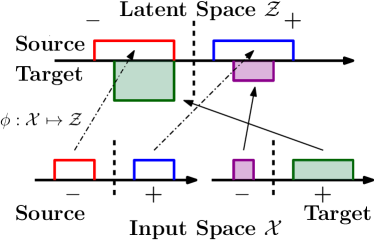
(a) Failure case

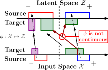
(b) Failure impossible

Figure 2: (a) Label consistency is broken even if $\phi$ satisfies the relaxed distribution aligning requirement. (b) The main idea of our analysis: A continuous mapping cannot project a connected region into two regions separated by a margin. So label consistency is preserved for a region that is connected to the source domain.

4.2 Example of a perfect target domain classifier

To interpret our result, we construct a simple situation where $\mathcal{E}_{T}(\phi,h)=0$ is guaranteed when the domain adversarial objective with relaxed distribution alignment is minimized to zero, exploiting pure data-dependent assumptions:

Assumption 4.4.

Assume the target support consists of disjoint clusters $\mathrm{Supp}(p_{T})=S_{T,0,1}\cup...\cup S_{T,0,m_{0}}\cup S_{T,1,1}\cup...\cup S_{T,1,m_{1}}$, where any cluster $S_{T,i,j}$ is connected and its labels are consistent: $f(x)=i$ for all $x\in S_{T,i,j}$. Moreover, each of these cluster overlaps with source distribution. That is, for any $i\in\{0,1\}$ and $j\in\{1,...,m_{i}\}$, $S_{T,i,j}\cap\mathrm{Supp}(p_{S})\neq\emptyset$.

Corollary 4.5.

If Assumption 4.4 holds and there exists a continuous mapping $\phi$ such that (i) $\sup_{z\in\mathcal{Z}}p_{T}^{\phi}(z)/p_{S}^{\phi}(z)\leq 1+\beta$ for some $\beta\geq 0$; (ii) for any pair $x_{0},x_{1}\in\mathrm{Supp}(p_{S})$ such that $f(x_{0})=0$ and $f(x_{1})=1$, we have $d_{\mathcal{Z}}(\phi(x_{0}),\phi(x_{1}))\geq\Delta>0$, then $\mathcal{E}_{S}(\phi,h)=0$ indicates $\mathcal{E}_{T}(\phi,h)=0$.

Proof follows directly by observing that a construction of $\delta_{1}=\delta_{2}=\delta_{3}=0$ exists in Theorem 4.3. A simple example that satisfies Assumption 4.4 is Figure 2(b). For a real world example, consider the cat-dog classification problem. Say that source domain contains small-to-medium cats and dogs while target domain contains medium-to-large cats and dogs. The target domain consists of clusters (e.g. cats and dogs, or multiple sub-categories) and each of them overlaps with the source domain (the medium ones).

5 Asymmetrically-relaxed distances

So far, we have motivated the use of asymmetrically-relaxed distribution alignment which aims at bounding $p_{T}^{\phi}/p_{S}^{\phi}$ by a constant instead of driving towards $p_{S}^{\phi}\equiv p_{T}^{\phi}$. More specifically, we propose to use a $\beta$-admissible (Definition 3.3) distance $D_{\beta}$ in objective (4) to align the source and target encodings rather than the standard distances corresponding an adversarial domain classifier. In this section, we derive several $\beta$-admissible distance metrics that can be practically minimized with adversarial training. More specifically, we propose three types of distances (i) f-divergences; (ii) modified Wasserstein distance; (iii) reweighting distances; and demonstrate how to optimize them by adversarial training.

5.1 $f$-divergence

Given a convex and continuous function $f$ which satisfies $f(1)=0$, the $f$-divergence between two distributions $p$ and $q$ can be written as $D_{f}(p,q)=\int\mathrm{d}zp(z)f\left(\frac{q(z)}{p(z)}\right)$. According to Jensen’s inequality $D_{f}(p,q)\geq f\left(\int\mathrm{d}zp(z)\frac{q(z)}{p(z)}\right)=0$. Standard choices of $f$ (see a list in Nowozin et al. (2016)) are strictly convex thus $D_{f}(p,q)=0$ if and only if $p\equiv q$ when $f$ is strictly convex. To derive a $\beta$-adimissible variation for each standard choice of $f$, we linearize $f(u)$ where $u\geq\frac{1}{1+\beta}$. If and only if $\frac{p(z)}{q(z)}\leq 1+\beta$ for all $z$, $f$ becomes a linear function with respect to all $q(z)/p(z)$ and thus Jensen’s inequality holds with equality.

Given a convex, continuous function $f:\mathbb{R}^{+}\mapsto\mathbb{R}$ with $f(1)=0$ and some $\beta\geq 0$, we introduce the partially linearized $\bar{f}_{\beta}$ as follows

$$\bar{f}_{\beta}(u)=\begin{cases}f(u)+C_{f,\beta}&\text{ if }u\leq\frac{1}{1+\beta}\,,\\ f^{\prime}(\frac{1}{1+\beta})u-f^{\prime}(\frac{1}{1+\beta})&\text{ if }u>\frac{1}{1+\beta}\,.\end{cases}$$

where $C_{f,\beta}=-f(\frac{1}{1+\beta})+f^{\prime}(\frac{1}{1+\beta})\frac{1}{1+\beta}-f^{\prime}(\frac{1}{1+\beta})$.

It can be shown that $\bar{f}_{\beta}$ is continuous, convex and $\bar{f}_{\beta}(1)=0$. As we already explained, $D_{\bar{f}_{\beta}}(p,q)=0$ if and only if $\frac{p(z)}{q(z)}\leq 1+\beta$ for all $z$. Hence is $D_{\bar{f}_{\beta}}$ is $\beta$-admissible.

Adversarial training According to Nowozin et al. (2016), adversarial training (Goodfellow et al., 2014) can be viewed as minimizing the dual form of $f$-divergences

$$D_{f}(p,q)=\sup_{T:\mathcal{Z}\mapsto\mathrm{dom}(f^{*})}\mathbb{E}_{z\sim q}\left[T(z)\right]-\mathbb{E}_{z\sim p}\left[f^{*}(T(z))\right]$$

where $f^{*}$ is the Fenchel Dual of $f$ with $f^{*}(t)=\sup_{u\in\mathrm{dom}(f)}\left\{ut-f(u)\right\}$. Applying the same derivation for $\bar{f}_{\beta}$ we get

$$D_{\bar{f}_{\beta}}(p,q)=\sup_{T:\mathcal{Z}\mapsto\mathrm{dom}(\bar{f}_{\beta}^{*})}\mathbb{E}_{z\sim q}\left[T(z)\right]-\mathbb{E}_{z\sim p}\left[f^{*}(T(z))\right]$$ (6)

where $\mathrm{dom}(\bar{f}_{\beta}^{*})=\mathrm{dom}(f^{*})\cap\big{(}-\infty,f^{\prime}(\frac{1}{1+\beta})\big{]}$.

Plugging in the corresponding $f$ for JS-divergence gives

$$D_{\bar{f}_{\beta}}(p,q)$$

$$=\sup_{g:\mathcal{Z}\mapsto(0,1]}\mathbb{E}_{z\sim q}\left[\log\frac{g(z)}{2+\beta}\right]+\mathbb{E}_{z\sim p}\left[\log\left(1-\frac{g(z)}{2+\beta}\right)\right]\,,$$ (7)

where $g(z)$ can be parameterized by a neural network with sigmoid output as typically used in adversarial training.

5.2 Wasserstein distance

The idea behind modifying the Wasserstein distance is to model the optimal transport from $p$ to the region where distributions have $1+\beta$ maximal density ratio with respect to $q$. We define the relaxed Wassertein distance as

$$W_{\beta}(p,q)=\inf_{\gamma\in\prod_{\beta}(p,q)}\mathbb{E}_{(z_{1},z_{2})\sim\gamma}\left[\left\lVert z_{1}-z_{2}\right\rVert\right]\,,$$

where $\prod_{\beta}(p,q)$ is defined as the set of joint distributions $\gamma$ over $\mathcal{Z}\times\mathcal{Z}$ such that

$$\forall z_{1}\int\mathrm{d}z\gamma(z_{1},z)=p(z_{1})\,;\forall z_{2}\int\mathrm{d}z\gamma(z,z_{2})\leq(1+\beta)q(z_{2})\,.$$

$W_{\beta}$ is $\beta$-admissible since no transportation is needed if $p$ already lies in the qualified region with respect to $q$.

Adversarial training Following the derivation for the original Wasserstein distance, the dual form becomes

$$W_{\beta}(p,q) =\sup_{g}\mathbb{E}_{z\sim p}\left[g(z)\right]-(1+\beta)\mathbb{E}_{z\sim q}\left[g(z)\right]$$ (8)

s.t. $$\forall z\in\mathcal{Z}\,,g(z)\geq 0\,,$$

$$\forall z_{1},z_{2}\in\mathcal{Z}\,,g(z_{1})-g(z_{2})\leq\left\lVert z_{1}-z_{2}\right\rVert\,,$$

Optimization with adversarial training can be done by parameterizing $g$ as a non-negative function (e.g. with soft-plus output $\log(1+e^{x})$ or RELU output $\max(0,x)$) and following Arjovsky et al. (2017); Gulrajani et al. (2017) to enforce its Lipschitz continuity approximately.

5.3 Reweighting distance

Given any distance metric $D$, a generic way to make it $\beta$-admissible is to allow reweighting for one of the distances within a $\beta$-dependent range. The relaxed distance is then defined as the minimum achievable distance by such reweighting.

Given a distribution $q$ over $\mathcal{Z}$ and a reweighting function $w:\mathcal{Z}\mapsto[0,\infty)$. The reweighted distribution $q_{w}$ is defined as $q_{w}(z)=\frac{q(z)w(z)}{\int\mathrm{d}zq(z)w(z)}$. Define $\mathcal{W}_{\beta,q}$ to be a set of $\beta$-qualified reweighting with respect to $q$:

$$\mathcal{W}_{\beta,q}=\left\{w:\mathcal{Z}\mapsto[0,1],\int\mathrm{d}zq(z)w(z)=\frac{1}{1+\beta}\right\}\,.$$

Then the relaxed distance can be defined as

$$D_{\beta}(p,q)=\min_{w\in\mathcal{W}_{\beta,q}}D(p,q_{w})\,.$$ (9)

Such $D_{\beta}$ is $\beta$-admissible since the set $\{q_{w}:w\in\mathcal{W}_{\beta,q}\}$ is exactly the set of $p$ such that $\sup_{z\in\mathcal{Z}}p(z)/q(z)\leq 1+\beta$.

Adversarial training We propose an implicit-reweighting-by-sorting approach to optimize $D_{\beta}$ without parameterizing the function $w$ when $D$ can be optimized by adversarial training. Adversarially trainable $D$ shares a general form as

$$D(p,q)=\sup_{g\in\mathcal{G}}\mathbb{E}_{z\sim p}\left[f_{1}(g(z))\right]-\mathbb{E}_{z\sim q}\left[f_{2}(g(z))\right]\,,$$

where $f_{1}$ and $f_{2}$ are monotonically increasing functions. According to (9), the relaxed distance can be written as

$$D_{\beta}(p,q)=\min_{w}\sup_{g\in\mathcal{G}}\mathbb{E}_{z\sim p}\left[f_{1}(g(z))\right]-\mathbb{E}_{z\sim q_{w}}\left[f_{2}(g(z))\right]\,,$$

$$\text{ s.t. }w:\mathcal{Z}\mapsto[0,1]\,,\int\mathrm{d}zq(z)w(z)=\frac{1}{1+\beta}\,.$$ (10)

One step of alternating minimization on $D_{\beta}$, could consist of fixing $p,q,g$ and optimizing $w$. Then the problem becomes

$$\max_{w\in\mathcal{W}_{\beta,q}}\int\mathrm{d}zq(z)w(z)f_{2}(g(z))\,.$$ (11)

Observe that the optimal solution to (11) is to assign $w(z)=1$ for the $\frac{1}{1+\beta}$ fraction of $z$ from distribution $q$, where $f_{2}(g(z))$ take the largest values. Based on this observation, we propose to do the following sub-steps when optimizing (11) as an alternating minimization step: (i) Sample a minibatch of $z\sim q$; (ii) Sort these $z$ in descending order according to $f_{2}(g(z))$; (iii) Assign $w(z)=1$ to the first $\frac{1}{1+\beta}$ fraction of the list. Note that this optimization procedure is not justified in principle with mini-batch adversarial training but we found it to work well in our experiments.

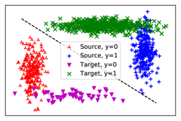
(a) raw (synthetic) data

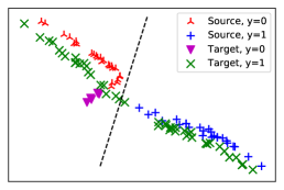
(b) latent representations (DANN)

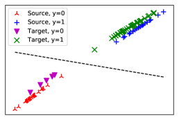
(c) latent representations (ours)

Figure 3: Domain-adversarial training under label distribution shift on a synthetic dataset.

6 Experiments

To evaluate our approach, we implement Domain Adversarial Neural Networks (DANN), (Ganin et al., 2016) replacing the JS-divergence (domain classifier) with our proposed $\beta$-admissible distances (Section 5). Our experiments address the following questions: (i) Does DANN suffer the limitation as anticipated (Section 3) when faced with label distribution shift? (ii) If so, do our $\beta$-admissible distances overcome these limitations? (iii) Absent shifting label distributions, is our approach comparable to DANN?

We implement adversarial training with different $\beta$-admissible distances (Section 5) and compare their performance with vanilla DANN. We name different implementations as follows. (a) Source: source-only training. (b) DANN: JS-divergence (original DANN). (c) WDANN: original Wasserstein distance. (d) fDANN-$\beta$: $\beta$-admissible $f$-divergence, JS-version (7). (e) sDANN-$\beta$: reweighting JS-divergence (10), optimized by our proposed implicit-reweighting-by-sorting. (f) WDANN1-$\beta$: $\beta$-admissible Wasserstein distance (8) with soft-plus on critic output. (g) WDANN2-$\beta$: $\beta$-admissible Wasserstein distance (8) with RELU on critic output. (h) sWDANN-$\beta$: reweighting Wasserstein distance (10), optimized by implicit-reweighting-by-sorting. Adversarial training on Wasserstein distances follows Gulrajani et al. (2017) but uses one-sided gradient-penalty. We always perform adversarial training with alternating minimization (see Appendix for details).

Synthetic datasets

We create a mixture-of-Gaussians binary classification dataset where each domain contains two Gaussian distributions, one per label. For each label, the distributions in source and target domain have a small overlap, validating the assumptions in our analysis. We create a label distribution shift with balanced source data (50% 0’s v.s. 50% 1’s) and imbalanced target data (10% 0’s v.s. 90% 1’s) as shown in Figure 3(a). Table 1 shows the target domain accuracy for different approaches. As expected, vanilla DANN fails under label distribution shift because a proportion of samples from the target inputs are mapped to regions of latent space corresponding to negative samples from the source domain (Figure 3(b)). In contrast, with our $\beta$-admissible distances, domain-adversarial networks are able to adapt successfully (Figure 3(c)), improving target accuracy from 89% (source-only) to 99% accuracy (with adaptation), except the cases where $\beta$ is too small to admit a good target domain classifier (in this case we need $\beta\geq 0.9/0.5-1=0.8$). We also experiment with label-balanced target data (no label distribution shift). All approaches except source-only achieve an accuracy above 99%, so we do not present these results in a separate table.

Table 1: Classification accuracy on target domain with label distribution shift on a synthetic dataset.

method	accuracy%
Source	89.4$\pm$1.1
DANN	59.1$\pm$5.1	WDANN	50.8$\pm$32.1
$\beta$	0.5	2.0	4.0
fDANN-$\beta$	66.0$\pm$ 41.6	99.9$\pm$ 0.0	99.8$\pm$0.0
sDANN-$\beta$	99.9$\pm$ 0.1	99.9$\pm$ 0.0	99.9$\pm$0.0
WDANN1-$\beta$	45.7$\pm$ 41.5	66.4$\pm$ 41.1	99.9$\pm$0.0
WDANN2-$\beta$	97.6$\pm$ 1.2	99.7$\pm$ 0.2	99.5$\pm$0.3
sWDANN-$\beta$	79.0$\pm$ 5.9	99.9$\pm$ 0.0	99.9$\pm$0.0

Real datasets

We experiment with the MNIST and USPS handwritten-digit datasets. For both directions (MNIST $\rightarrow$ USPS and USPS $\rightarrow$ MNIST), we experiment both with and without label distribution shift. The source domain is always class-balanced. To simulate label distribution shift, we sample target data from only half of the digits, e.g. [0-4] or [5-9]. Tables 2 and 3 show the target domain accuracy for different approaches with/without label distribution shift. As on synthetic datasets, we observe that DANN performs much worse than source-only training under label distribution shift. Compared to the original DANN, our approaches fair significantly better while achieving comparable performance absent label distribution shift.

Table 2: Classification accuracy on target domain with/without label distribution shift on MNIST-USPS.

target	[0-4]	[5-9]	[0-9]
labels	Shift	Shift	No-Shift
Source	74.3$\pm$1.0	59.5$\pm$3.0	66.7$\pm$2.1
DANN	50.0$\pm$1.9	28.2$\pm$2.8	78.5$\pm$1.6
fDANN-$1$	71.6$\pm$4.0	67.5$\pm$2.3	73.7$\pm$1.5
fDANN-$2$	74.3$\pm$2.5	61.9$\pm$2.9	72.6$\pm$0.9
fDANN-$4$	75.9$\pm$1.6	64.4$\pm$3.6	72.3$\pm$1.2
sDANN-$1$	71.6$\pm$3.7	49.1$\pm$6.3	81.0$\pm$1.3
sDANN-$2$	76.4$\pm$3.1	48.7$\pm$9.0	81.7$\pm$1.4
sDANN-$4$	81.0$\pm$1.6	60.8$\pm$7.5	82.0$\pm$0.4

Table 3: Classification accuracy on target domain with/without label distribution shift on USPS-MNIST.

target	[0-4]	[5-9]	[0-9]
labels	Shift	Shift	No-Shift
Source	69.4$\pm$2.3	30.3$\pm$2.8	49.4$\pm$2.1
DANN	57.6$\pm$1.1	37.1$\pm$3.5	81.9$\pm$6.7
fDANN-$1$	80.4$\pm$2.0	40.1$\pm$3.2	75.4$\pm$4.5
fDANN-$2$	86.6$\pm$4.9	41.7$\pm$6.6	70.0$\pm$3.3
fDANN-$4$	77.6$\pm$6.8	34.7$\pm$7.1	58.5$\pm$2.2
sDANN-$1$	68.2$\pm$2.7	45.4$\pm$7.1	78.8$\pm$5.3
sDANN-$2$	78.6$\pm$3.6	36.1$\pm$5.2	77.4$\pm$5.7
sDANN-$4$	83.5$\pm$2.7	41.1$\pm$6.6	75.6$\pm$6.9

7 Related work

Our paper makes distinct theoretical and algorithmic contributions to the domain adaptation literature. Concerning theory, we provide a risk bound that explains the behavior of domain-adversarial methods with model-independent assumptions on data distributions. Existing theories without assumptions of contained support (Ben-David et al., 2007, 2010a; Ben-David & Urner, 2014; Mansour et al., 2009; Cortes & Mohri, 2011) do not exhibit this property since (i) when applied to the input space, their results are not concerned with domain-adversarial learning as no latent space is introduced, (ii) when applied to the latent space, their unobservable constants/assumptions become $\phi$-dependent, which is undesirable as explained in Section 4. Concerning algorithms, several prior works demonstrate empirical success of domain-adversarial approaches, (Tzeng et al., 2014; Ganin et al., 2016; Bousmalis et al., 2016; Tzeng et al., ; Hoffman et al., 2017; Shu et al., 2018). Among those, Cao et al. (2018a, b) deal with the label distribution shift scenario through a heuristic reweighting scheme. However, their re-weighting presumes that they have a good classifier in the first place, creating a cyclic dependency.

8 Conclusions

We propose to use asymmetrically-relaxed distribution distances in domain-adversarial learning objectives, replacing standard ones which seek exact distribution matching in the latent space. While overcoming some limitations of the standard objectives under label distribution mismatch, we provide a theoretical guarantee for target domain performance under assumptions on data distributions. As our connectedness assumptions may not cover all cases where we expect domain adaptation to work in practice, (e.g. when the two domains are completely disjoint), providing analysis under other type of assumptions might be of future interest.

Acknowledgments

This work was made possible by a generous grant from the Center for Machine Learning and Health, a joint venture of Carnegie Mellon University, UPMC, and the University of Pittsburgh, in support of our collaboration with Abridge AI to develop robust models for machine learning in healthcare. We are also supported in this line of research by a generous faculty award from Salesforce Research.

Appendix A Proofs

Derivation of (1).

$$\mathcal{E}_{U}(\phi,h) =\int\mathrm{d}xp_{U}(x)\left\lvert h(\phi(x))-f(x)\right\rvert$$

$$=\int\mathrm{d}x\int\mathrm{d}zp_{U}^{\phi}(z)\phi_{U}(x|z)\left\lvert h(\phi(x))-f(x)\right\rvert$$

$$=\int\mathrm{d}zp_{U}^{\phi}(z)\int\mathrm{d}x\phi_{U}(x|z)\left\lvert h(z)-f(x)\right\rvert$$

$$=\int\mathrm{d}zp_{U}^{\phi}(z)\left\lvert h(z)-\int\mathrm{d}x\phi_{U}(x|z)f(x)\right\rvert$$

$$\doteq\int\mathrm{d}zp_{U}^{\phi}(z)\left\lvert h(z)-f^{\phi}_{U}(z)\right\rvert$$

$$\doteq\int\mathrm{d}zp_{U}^{\phi}(z)r_{U}(z;\phi,h)$$

where we use the following fact: For any fixed $z$, $h(z)\in\{0,1\}$, if $h(z)=0$ then $|h(z)-f(x)|=f(x)-h(z)$ for all $x$. Similarly, when $h(z)=1$, we have $|h(z)-f(x)|=h(z)-f(x)$ for all $x$. Thus we can move the integral over $x$ inside the absolute operation. ∎

Proof of Proposition 3.1.

First we have

$$\rho_{U}=\int\mathrm{d}xp_{U}(x)f(x)=\int\mathrm{d}x\int\mathrm{d}zp_{U}^{\phi}(z)\phi_{U}(x|z)f(x)=\int\mathrm{d}zp_{U}^{\phi}(z)f_{U}^{\phi}(z)\,.$$

When $\mathcal{E}_{S}(\phi,h)=0$ we have

$$\left\lvert\int\mathrm{d}zp_{S}^{\phi}(z)h(z)-\rho_{S}\right\rvert=\left\lvert\int\mathrm{d}zp_{S}^{\phi}(z)h(z)-\int\mathrm{d}zp_{S}^{\phi}(z)f_{S}^{\phi}(z)\right\rvert\leq\int\mathrm{d}zp_{S}^{\phi}(z)\left\lvert h(z)-f_{S}^{\phi}(z)\right\rvert=\mathcal{E}_{S}(\phi,h)=0$$

thus $\int\mathrm{d}zp_{S}^{\phi}(z)h(z)=\rho_{S}$.

Applying the fact that $p_{S}^{\phi}(z)=p_{T}^{\phi}(z)$ for all $z\in\mathcal{Z}$,

$$\mathcal{E}_{T}(\phi,h)=\int\mathrm{d}zp_{T}^{\phi}(z)\left\lvert h(z)-f_{T}^{\phi}(z)\right\rvert\geq\left\lvert\int\mathrm{d}zp_{T}^{\phi}(z)h(z)-\int\mathrm{d}zp_{T}^{\phi}(z)f_{T}^{\phi}(z)\right\rvert$$

$$=\left\lvert\int\mathrm{d}zp_{S}^{\phi}(z)h(z)-\int\mathrm{d}zp_{T}^{\phi}(z)f_{T}^{\phi}(z)\right\rvert=\left\lvert\rho_{S}-\rho_{T}\right\rvert\,,$$

which concludes the proof. ∎

Proof of Proposition 3.2.

Let $p_{S}$ be the uniform distribution over $[0,1]$ and $p_{T}$ be the uniform distribution over $[2,3]$. The labeling function $f$ is set as $f(x)=1$ iff $x\in[0,\rho_{S}]\cup[2,2+\rho_{T}]$ such that the definition of $\rho_{S}$ and $\rho_{T}$ is preserved. We construct the following mapping $\phi$: For $x\in[0,1]$ $\phi(x)=x$. For $x\in[2,2+\rho_{T}]$ $\phi(x)=(x-2)\rho_{S}/\rho_{T}$. For $x\in[2+\rho_{T},3]$ $\phi(x)=1-(3-x)(1-\rho_{S})/(1-\rho_{T})$. $\phi$ maps both source and target data into $[0,1]$ with $p_{S}^{\phi}$ to be uniform over $[0,1]$ and $p_{T}^{\phi}(z)=\rho_{T}/\rho_{S}$ when $z\in[0,\rho_{S}]$ and $p_{T}^{\phi}(z)=(1-\rho_{T})/(1-\rho_{S})$ when $z\in[\rho_{S},1]$. Since $p_{S}^{\phi}(z)=1$ for all $z\in[0,1]$ we can conclude that $\sup_{z\in\mathcal{Z}}p_{T}^{\phi}(z)/p_{S}^{\phi}(z)\leq\max\left\{\frac{\rho_{T}}{\rho_{S}},\frac{1-\rho_{T}}{1-\rho_{S}}\right\}$ . ∎

Proof of Theorem 4.3.

Instead of working with Assumption 4.2 we first extend Construction 4.1 with the following addition

Construction A.1.

(Connectedness from target domain to source domain.) Let $C_{T}\subset\mathcal{X}$ be a set of points in the raw data space that satisfy the following conditions:

1. $\phi(C_{T})\subset\phi(C_{0}\cup C_{1})$.

2. For any $x\in C_{T}$, there exists $x^{\prime}\in C_{T}\cap(C_{0}\cup C_{1})$ such that one can find a sequence of points $x_{0},x_{1},...,x_{m}\in C_{T}$ with $x_{0}=x$, $x_{m}=x^{\prime}$, $f(x)=f(x^{\prime})$ and $d_{\mathcal{X}}(x_{i-1},x_{i})<\frac{\Delta}{L}$ for all $i=1,...,m$.

3. $p_{T}(C_{T})\geq 1-\delta_{3}$.

We now proceed to prove bound based on Constructions 4.1 and A.1. Later on we will show that Assumption 4.2 indicates the existence of Construction A.1 so that the bound holds with a combination of Constructions 4.1 and Assumption 4.2.

The third term of (2) can be written as

$$\int\mathrm{d}zp_{S}^{\phi}(z)\left(\frac{p_{T}^{\phi}(z)}{p_{S}^{\phi}(z)}-1\right)r_{S}(z;\phi,h)$$

$$\leq\inf_{B\subseteq\mathcal{Z}}\int_{B}\mathrm{d}zp_{S}^{\phi}(z)\left(\frac{p_{T}^{\phi}(z)}{p_{S}^{\phi}(z)}-1\right)r_{S}(z;\phi,h)+\int_{B^{c}}\mathrm{d}zp_{S}^{\phi}(z)\left(\frac{p_{T}^{\phi}(z)}{p_{S}^{\phi}(z)}-1\right)r_{S}(z;\phi,h)$$

$$\leq\inf_{B\subseteq\mathcal{Z}}\left(\sup_{z\in B}\frac{p_{T}^{\phi}(z)}{p_{S}^{\phi}(z)}-1\right)\int_{B}\mathrm{d}zp_{S}^{\phi}(z)r_{S}(z;\phi,h)+\int_{B^{c}}\mathrm{d}zp_{T}^{\phi}(z)r_{S}(z;\phi,h)$$

$$\leq\inf_{B\subseteq\mathcal{Z}}\left(\sup_{z\in B}\frac{p_{T}^{\phi}(z)}{p_{S}^{\phi}(z)}-1\right)\mathcal{E}_{S}(\phi,h)+p_{T}^{\phi}(B^{c})$$

$$\leq\beta\mathcal{E}_{S}(\phi,h)+\delta_{1}\,.$$ (12)

For the second term of (2), plugging in $r_{U}(z;\phi,h)=\left\lvert h(z)-f^{\phi}_{U}(z)\right\rvert$ gives

$$\int\mathrm{d}zp_{T}^{\phi}(z)\left(r_{T}(z;\phi,h)-r_{S}(z;\phi,h)\right)$$

$$=\int\mathrm{d}zp_{T}^{\phi}(z)\left(\left\lvert h(z)-f^{\phi}_{T}(z)\right\rvert-\left\lvert h(z)-f^{\phi}_{S}(z)\right\rvert\right)$$

$$=\int\mathrm{d}zp_{T}^{\phi}(z)\left\lvert f^{\phi}_{T}(z)-f^{\phi}_{S}(z)\right\rvert$$

$$=\int\mathrm{d}zp_{T}^{\phi}(z)\left\lvert f^{\phi}_{T}(z)-f^{\phi}_{S}(z)\right\rvert\left(\mathbbm{1}\left\{z\in\phi(C_{0})\right\}+\mathbbm{1}\left\{z\in\phi(C_{1})\right\}+\mathbbm{1}\left\{z\in\left(\phi(C_{0})\cup\phi(C_{1})\right)^{c}\right\}\right)$$

$$=\int\mathrm{d}zp_{T}^{\phi}(z)\left\lvert f^{\phi}_{T}(z)-f^{\phi}_{S}(z)\right\rvert\mathbbm{1}\left\{z\in\phi(C_{0})\right\}+\int\mathrm{d}zp_{T}^{\phi}(z)\left\lvert f^{\phi}_{T}(z)-f^{\phi}_{S}(z)\right\rvert\mathbbm{1}\left\{z\in\phi(C_{1})\right\}$$

$$+\int\mathrm{d}zp_{T}^{\phi}(z)\left\lvert f^{\phi}_{T}(z)-f^{\phi}_{S}(z)\right\rvert\mathbbm{1}\left\{z\in\left(\phi(C_{0})\cup\phi(C_{1})\right)^{c}\right\}$$ (13)

Applying $\left\lvert f^{\phi}_{T}(z)-f^{\phi}_{S}(z)\right\rvert\leq f^{\phi}_{T}(z)+f^{\phi}_{S}(z)$ to the first part of (13) gives

$$\int\mathrm{d}zp_{T}^{\phi}(z)\left\lvert f^{\phi}_{T}(z)-f^{\phi}_{S}(z)\right\rvert\mathbbm{1}\left\{z\in\phi(C_{0})\right\}$$

$$\leq\int\mathrm{d}zp_{T}^{\phi}(z)f^{\phi}_{T}(z)\mathbbm{1}\left\{z\in\phi(C_{0})\right\}+\int\mathrm{d}zp_{T}^{\phi}(z)f^{\phi}_{S}(z)\mathbbm{1}\left\{z\in\phi(C_{0})\right\}$$

$$=\int\mathrm{d}zp_{T}^{\phi}(z)\int\mathrm{d}x\phi_{T}(x|z)f(x)\mathbbm{1}\left\{z\in\phi(C_{0})\right\}+\int\mathrm{d}zp_{T}^{\phi}(z)f^{\phi}_{S}(z)\mathbbm{1}\left\{z\in\phi(C_{0})\right\}$$

$$=\int\mathrm{d}xf(x)\int\mathrm{d}zp_{T}^{\phi}(z)\phi_{T}(x|z)\mathbbm{1}\left\{z\in\phi(C_{0})\right\}+\int\mathrm{d}zp_{T}^{\phi}(z)f^{\phi}_{S}(z)\mathbbm{1}\left\{z\in\phi(C_{0})\right\}$$

$$=\int\mathrm{d}xf(x)p_{T}(x)\mathbbm{1}\left\{\phi(x)\in\phi(C_{0})\right\}+\int\mathrm{d}zp_{T}^{\phi}(z)f^{\phi}_{S}(z)\mathbbm{1}\left\{z\in\phi(C_{0})\right\}$$

$$=\int\mathrm{d}xp_{T}(x)\mathbbm{1}\left\{f(x)=1,\phi(x)\in\phi(C_{0})\right\}+\int\mathrm{d}zp_{T}^{\phi}(z)f^{\phi}_{S}(z)\mathbbm{1}\left\{z\in\phi(C_{0})\right\}$$ (14)

Similarly, applying $\left\lvert f^{\phi}_{T}(z)-f^{\phi}_{S}(z)\right\rvert=\left\lvert(1-f^{\phi}_{T}(z))-(1-f^{\phi}_{S}(z))\right\rvert\leq(1-f^{\phi}_{T}(z))+(1-f^{\phi}_{S}(z))$ to the second part of (13) gives

$$\int\mathrm{d}zp_{T}^{\phi}(z)\left\lvert f^{\phi}_{T}(z)-f^{\phi}_{S}(z)\right\rvert\mathbbm{1}\left\{z\in\phi(C_{1})\right\}$$

$$\leq\int\mathrm{d}zp_{T}^{\phi}(z)(1-f^{\phi}_{T}(z))\mathbbm{1}\left\{z\in\phi(C_{1})\right\}+\int\mathrm{d}zp_{T}^{\phi}(z)(1-f^{\phi}_{S}(z))\mathbbm{1}\left\{z\in\phi(C_{1})\right\}$$

$$=\int\mathrm{d}zp_{T}^{\phi}(z)\left(1-\int\mathrm{d}x\phi_{T}(x|z)f(x)\right)\mathbbm{1}\left\{z\in\phi(C_{1})\right\}+\int\mathrm{d}zp_{T}^{\phi}(z)(1-f^{\phi}_{S}(z))\mathbbm{1}\left\{z\in\phi(C_{1})\right\}$$

$$=\int\mathrm{d}x(1-f(x))\int\mathrm{d}zp_{T}^{\phi}(z)\phi_{T}(x|z)\mathbbm{1}\left\{z\in\phi(C_{1})\right\}+\int\mathrm{d}zp_{T}^{\phi}(z)(1-f^{\phi}_{S}(z))\mathbbm{1}\left\{z\in\phi(C_{1})\right\}$$

$$=\int\mathrm{d}x(1-f(x))p_{T}(x)\mathbbm{1}\left\{\phi(x)\in\phi(C_{1})\right\}+\int\mathrm{d}zp_{T}^{\phi}(z)(1-f^{\phi}_{S}(z))\mathbbm{1}\left\{z\in\phi(C_{1})\right\}$$

$$=\int\mathrm{d}xp_{T}(x)\mathbbm{1}\left\{f(x)=0,\phi(x)\in\phi(C_{1})\right\}+\int\mathrm{d}zp_{T}^{\phi}(z)(1-f^{\phi}_{S}(z))\mathbbm{1}\left\{z\in\phi(C_{1})\right\}$$ (15)

Combining the second part of (14) and the second part of (15)

$$\int\mathrm{d}zp_{T}^{\phi}(z)f^{\phi}_{S}(z)\mathbbm{1}\left\{z\in\phi(C_{0})\right\}+\int\mathrm{d}zp_{T}^{\phi}(z)(1-f^{\phi}_{S}(z))\mathbbm{1}\left\{z\in\phi(C_{1})\right\}$$

$$=\int\mathrm{d}z\frac{p_{T}^{\phi}(z)}{p_{S}^{\phi}(z)}p_{S}^{\phi}(z)f^{\phi}_{S}(z)\mathbbm{1}\left\{z\in\phi(C_{0})\right\}\left(\mathbbm{1}\left\{z\in B\right\}+\mathbbm{1}\left\{z\in B^{c}\right\}\right)$$

$$+\int\mathrm{d}z\frac{p_{T}^{\phi}(z)}{p_{S}^{\phi}(z)}p_{S}^{\phi}(z)(1-f^{\phi}_{S}(z))\mathbbm{1}\left\{z\in\phi(C_{1})\right\}\left(\mathbbm{1}\left\{z\in B\right\}+\mathbbm{1}\left\{z\in B^{c}\right\}\right)$$

$$\leq(1+\beta)\int\mathrm{d}zp_{S}^{\phi}(z)f^{\phi}_{S}(z)\mathbbm{1}\left\{z\in\phi(C_{0})\right\}+(1+\beta)\int\mathrm{d}zp_{S}^{\phi}(z)(1-f^{\phi}_{S}(z))\mathbbm{1}\left\{z\in\phi(C_{1})\right\}$$

$$+\int\mathrm{d}zp_{T}^{\phi}(z)\mathbbm{1}\left\{z\in B^{c}\right\}\left(\mathbbm{1}\left\{z\in\phi(C_{0})\right\}+\mathbbm{1}\left\{z\in\phi(C_{1})\right\}\right)$$

$$\leq(1+\beta)\int\mathrm{d}xp_{S}(x)\mathbbm{1}\left\{f(x)=1,\phi(x)\in\phi(C_{0})\right\}+(1+\beta)\int\mathrm{d}xp_{S}(x)\mathbbm{1}\left\{f(x)=0,\phi(x)\in\phi(C_{1})\right\}+p_{T}(B^{c})$$

$$\leq(1+\beta)\int\mathrm{d}xp_{S}(x)\left(\mathbbm{1}\left\{f(x)=1,\phi(x)\in\phi(C_{0})\lor f(x)=0,\phi(x)\in\phi(C_{1})\right\}\right)+\delta_{1}$$ (16)

For $i\in\{0,1\}$ if $x\in C_{i}$ then $f(x)=i$ and $\phi(x)\in C_{i}$. So if $f(x)=1,\phi(x)\in\phi(C_{0})$ or $f(x)=0,\phi(x)\in\phi(C_{1})$ holds we must have $x\notin C_{0}\cup C_{1}$. Therefore, following (16) gives

$$\int\mathrm{d}zp_{T}^{\phi}(z)f^{\phi}_{S}(z)\mathbbm{1}\left\{z\in\phi(C_{0})\right\}+\int\mathrm{d}zp_{T}^{\phi}(z)(1-f^{\phi}_{S}(z))\mathbbm{1}\left\{z\in\phi(C_{1})\right\}$$

$$\leq(1+\beta)\int\mathrm{d}xp_{S}(x)\mathbbm{1}\left\{x\notin C_{0}\cup C_{1}\right\}+\delta_{1}$$

$$=(1+\beta)(1-p_{S}(C_{0}\cup C_{1}))+\delta_{1}$$

$$\leq(1+\beta)\delta_{2}+\delta_{1}$$ (17)

Now looking at the first part of (14) and the first part of (15)

$$\int\mathrm{d}xp_{T}(x)\mathbbm{1}\left\{f(x)=1,\phi(x)\in\phi(C_{0})\right\}+\int\mathrm{d}xp_{T}(x)\mathbbm{1}\left\{f(x)=0,\phi(x)\in\phi(C_{1})\right\}$$

$$=\int\mathrm{d}xp_{T}(x)\mathbbm{1}\left\{f(x)=1,\phi(x)\in\phi(C_{0}),x\in C_{T}\right\}+\int\mathrm{d}xp_{T}(x)\mathbbm{1}\left\{f(x)=1,\phi(x)\in\phi(C_{0}),x\notin C_{T}\right\}$$

$$+\int\mathrm{d}xp_{T}(x)\mathbbm{1}\left\{f(x)=0,\phi(x)\in\phi(C_{1}),x\in C_{T}\right\}+\int\mathrm{d}xp_{T}(x)\mathbbm{1}\left\{f(x)=0,\phi(x)\in\phi(C_{1}),x\notin C_{T}\right\}$$

$$\leq\int\mathrm{d}xp_{T}(x)\left(\mathbbm{1}\left\{f(x)=1,\phi(x)\in\phi(C_{0}),x\in C_{T}\right\}+\mathbbm{1}\left\{f(x)=0,\phi(x)\in\phi(C_{1}),x\in C_{T}\right\}\right)+p_{T}(C_{T}^{c})$$

$$\leq\int\mathrm{d}xp_{T}(x)\mathbbm{1}\left\{x\in C_{T}\right\}\mathbbm{1}\left\{f(x)=1,\phi(x)\in\phi(C_{0})\lor f(x)=0,\phi(x)\in\phi(C_{1})\right\}+\delta_{3}\,.$$ (18)

Next we show that the first part of (18) is $0$. Recall that $\phi(C_{T})\subset\phi(C_{0}\cup C_{1})$ and if $x\in C_{T}$ there exists $x^{\prime}\in C_{T}\cap(C_{0}\cup C_{1})$ with a sequence of points $x_{0},x_{1},...,x_{m}\in C_{T}$ such that $x_{0}=x$, $x_{m}=x^{\prime}$, $f(x)=f(x^{\prime})$ and $d_{\mathcal{X}}(x_{i-1},x_{i})<\frac{\Delta}{L}$ for all $i=1,...,m$. So for $x\in C_{T}$ and $f(x)=i$, we pick such $x^{\prime}$. Since $\phi$ is $L$-Lipschitz and $\phi(C_{T})\subset\phi(C_{0}\cup C_{1})$ we have $\phi(x_{0}),\phi(x_{1}),...,\phi(x_{m})\in\phi(C_{0}\cup C_{1})$ and $d_{\mathcal{Z}}(\phi(x_{i-1}),\phi(x_{i}))<\Delta$ for all $i=1,...,m$. Applying the fact that $\inf_{z_{0}\in\phi(C_{0}),z_{1}\in\phi(C_{1})}d_{\mathcal{Z}}(z_{0},z_{1})\geq\Delta>0$ we know that if $\phi(x)=\phi(x_{0})\in\phi(C_{j})$ for some $j\in\{0,1\}$ then $\phi(x^{\prime})=\phi(x_{m})\in\phi(C_{j})$. From $x^{\prime}\in C_{0}\cup C_{1}$ and $f(x^{\prime})=f(x)=i$ we have $\phi(x^{\prime})\in\phi(C_{i})$. Since $C_{0}\cap C_{1}=\emptyset$ we can conclude $i=j$ and thus $\phi(x)\in\phi(C_{i})$ if $f(x)=i$ for any $x\in C_{T}$. Therefore, if $x\in C_{T}$, neither $f(x)=1,\phi(x)\in\phi(C_{0})$ nor $f(x)=0,\phi(x)\in\phi(C_{1})$ can hold. Hence the first part of (18) is $0$.

So far by combining (17) and (18) we have shown that the sum of (14) and (15) (which are the first two parts of (13)) can be upper bounded by $\delta_{1}+(1+\beta)\delta_{2}+\delta_{3}$. For the third part of (13) we have

$$\int\mathrm{d}zp_{T}^{\phi}(z)\left\lvert f^{\phi}_{T}(z)-f^{\phi}_{S}(z)\right\rvert\mathbbm{1}\left\{z\in\left(\phi(C_{0})\cup\phi(C_{1})\right)^{c}\right\}$$

$$\leq\int\mathrm{d}zp_{T}^{\phi}(z)\mathbbm{1}\left\{z\in\left(\phi(C_{0})\cup\phi(C_{1})\right)^{c}\right\}$$

$$=\int\mathrm{d}z\frac{p_{T}^{\phi}(z)}{p_{S}^{\phi}(z)}p_{S}^{\phi}(z)\mathbbm{1}\left\{z\in\left(\phi(C_{0})\cup\phi(C_{1})\right)^{c}\right\}\left(\mathbbm{1}\left\{z\in B\right\}+\mathbbm{1}\left\{z\in B^{c}\right\}\right)$$

$$\leq\int\mathrm{d}z\frac{p_{T}^{\phi}(z)}{p_{S}^{\phi}(z)}p_{S}^{\phi}(z)\mathbbm{1}\left\{z\in\left(\phi(C_{0})\cup\phi(C_{1})\right)^{c}\right\}\mathbbm{1}\left\{z\in B\right\}+\int\mathrm{d}zp_{T}^{\phi}(z)\mathbbm{1}\left\{z\in B^{c}\right\}$$

$$\leq(1+\beta)\int\mathrm{d}zp_{S}^{\phi}(z)\mathbbm{1}\left\{z\in\left(\phi(C_{0})\cup\phi(C_{1})\right)^{c}\right\}+\delta_{1}$$

$$=(1+\beta)\left(1-\int\mathrm{d}zp_{S}^{\phi}(z)\mathbbm{1}\left\{z\in\phi(C_{0})\cup\phi(C_{1})\right\}\right)+\delta_{1}$$

$$=(1+\beta)\left(1-\int\mathrm{d}xp_{S}(x)\mathbbm{1}\left\{x\in\phi^{-1}\left(\phi(C_{0})\cup\phi(C_{1})\right)\right\}\right)+\delta_{1}$$

$$=(1+\beta)\left(1-p_{S}\left(\phi^{-1}\left(\phi(C_{0})\cup\phi(C_{1})\right)\right)\right)+\delta_{1}$$

$$\leq(1+\beta)\left(1-p_{S}\left(C_{0}\cup C_{1}\right)\right)+\delta_{1}$$

$$\leq(1+\beta)\delta_{2}+\delta_{1}\,.$$ (19)

Putting (19) into (13) gives

$$\int\mathrm{d}zp_{T}^{\phi}(z)\left(r_{T}(z;\phi,h)-r_{S}(z;\phi,h)\right)\leq 2\delta_{1}+2(1+\beta)\delta_{2}+\delta_{3}\,.$$ (20)

Plugging (12) and (20) into (2) gives the result of Theorem 4.3 under Constructions 4.1 and  A.1.

It remains to show that Assumption 4.2 implies the existence of a Construction A.1. To prove this, we first write $\phi(C_{T})\subset\phi(C_{0}\cup C_{1})$ as $C_{T}\subset\phi^{-1}(\phi(C_{0}\cup C_{1}))$. By Construction 4.1 we have $p_{S}(C_{0}\cup C_{1})\geq 1-\delta_{2}$. From (19) we have

$$p_{T}\left(\phi^{-1}(\phi(C_{0}\cup C_{1}))\right)=\int\mathrm{d}xp_{T}(x)\mathbbm{1}\left\{x\in\phi^{-1}(\phi(C_{0}\cup C_{1}))\right\}$$

$$=\int\mathrm{d}zp_{T}^{\phi}(z)\mathbbm{1}\left\{z\in\phi(C_{0}\cup C_{1})\right\}\geq(1+\beta)\delta_{2}+\delta_{1}\,.$$

Setting $B_{S}=C_{0}\cup C_{1}$ and $B_{T}=\phi^{-1}(\phi(C_{0}\cup C_{1})$ in Assumption 4.2 gives a construction of Construction A.1, thus concluding the proof.

∎

Proof of Corollary 4.5.

Based on the statement of Corollary 4.5 it is obvious that Construction 4.1 can be made with $\delta_{1}=0$, $\delta_{2}=0$ and a finitely large $L$. (Here we implicitly assume that $\phi$ is bounded on $\mathcal{X}$). It remains to show that Assumption 4.2 holds with $\delta_{3}=0$. As $\delta_{1}=\delta_{2}=0$, any $B_{S}$ and $B_{T}$ will be supersets of $\mathrm{Supp}(p_{S})$ and $\mathrm{Supp}(p_{T})$ respectively. So it sufficies to consider $B_{S}=\mathrm{Supp}(p_{S})$ and $B_{T}=\mathrm{Supp}(p_{T})$.

Now we verify that $C_{T}=\mathrm{Supp}(p_{T})$ satisfies the requirements in Assumption 4.2. According to Assumption 4.4, for any $x\in\mathrm{Supp}(p_{T})$, there must exist $S_{T,i,j}$ such that $x\in S_{T,i,j}$, $S_{T,i,j}$ is connected, $f(x^{\prime})=i$ for all $x^{\prime}\in S_{T,i,j}$ and $S_{T,i,j}\cap\mathrm{Supp}(p_{S})\neq\emptyset$. Pick $x^{\prime}\in S_{T,i,j}\cap\mathrm{Supp}(p_{S})$. Such $x^{\prime}$ satisfies $x^{\prime}\in C_{T}\cap B_{S}$ with our choice of $C_{T}$ and $B_{S}$. Since $S_{T,i,j}$ is connected we can find a sequence of points $x_{0},...,x_{m}\in S_{T,i,j}$ with $x_{0}=0$, $x_{m}=x^{\prime}$ and $d_{\mathcal{X}}(x_{i-1},x_{i})<\epsilon$ for any $\epsilon>0$. As $S_{T,i,j}$ is label consistent we have $f(x)=f(x^{\prime})$. Picking $\epsilon=\frac{\Delta}{L}$ concludes the fact that $C_{T}=\mathrm{Supp}(p_{T})$ satisfies the requirements in Assumption 4.2.

Since $p_{T}(\mathrm{Supp}(p_{T}))=1$ we have $\delta_{3}=0$. As a result, $\mathcal{E}_{T}(\phi,h)\leq(1+\beta)\mathcal{E}_{S}(\phi,h)$ holds according to Theorem 4.3, which concludes the proof of Corollary 4.5.

∎

Derivation of (6).

The Fenchel Dual of $\bar{f}_{\beta}(u)$ can be written as

$$\bar{f}_{\beta}^{*}(t) =\begin{cases}tf^{\prime-1}(t)-\bar{f}_{\beta}(f^{\prime-1}(t))&\text{ if }t\leq f^{\prime}(\frac{1}{1+\beta})\,,\\ +\infty&\text{ if }t>f^{\prime}(\frac{1}{1+\beta})\,.\end{cases}$$

$$=\begin{cases}tf^{\prime-1}(t)-f(f^{\prime-1}(t))+C&\text{ if }t\leq f^{\prime}(\frac{1}{1+\beta})\,,\\ +\infty&\text{ if }t>f^{\prime}(\frac{1}{1+\beta})\,.\end{cases}$$

$$=\begin{cases}f^{*}(t)+C_{f,\beta}&\text{ if }t\leq f^{\prime}(\frac{1}{1+\beta})\,,\\ +\infty&\text{ if }t>f^{\prime}(\frac{1}{1+\beta})\,.\end{cases}\,,$$

where $C_{f,\beta}=f(\frac{1}{1+\beta})-f^{\prime}(\frac{1}{1+\beta})\frac{1}{1+\beta}+f^{\prime}(\frac{1}{1+\beta})$.

Therefore, the modified $\bar{f}_{\beta}$-divergence can be written as

$$D_{f,\beta}(p,q)=\sup_{T:\mathcal{Z}\mapsto\mathrm{dom}(f^{*})\cap(-\infty,f^{\prime}(\frac{1}{1+\beta})]}\mathbb{E}_{z\sim q}\left[T(z)\right]-\mathbb{E}_{z\sim p}\left[f^{*}(T(z))\right]-C_{f,\beta}\,.$$

∎

Derivation of (7).

According to Nowozin et al. (2016), the GAN objecitve uses $f(u)=u\log u-(1+u)\log(1+u)$. Hence $f^{*}(t)=-\log(1-e^{t})$, $f^{\prime}(u)=\log\frac{u}{u+1}$ and $f^{\prime}(\frac{1}{1+\beta})=\log\frac{1}{2+\beta}$. So we need to parameterize $T:\mathcal{Z}\mapsto\big{(}-\infty,\log\frac{1}{2+\beta}\big{]}$. $T(z)=\log\frac{g(z)}{2+\beta}$ with $g(z)\in(0,1]$ satisfies the range constraint for $T$. Plugging $T(z)=\log\frac{g(z)}{2+\beta}$ into (6) gives the result of (7).

∎

Appendix B Experiment Details

Synthetic datasets For source distribution, we sample class $0$ from $\mathcal{N}([-1,-0.3],diag(0.1,0.4))$ and class $1$ from $\mathcal{N}([1,0.3],diag(0.1,0.4))$. For target distribution, we sample class $0$ from $\mathcal{N}([-0.3,-1],diag(0.4,0.1))$ and class $1$ from $\mathcal{N}([0.3,1],diag(0.4,0.1))$. For label classifier, we use a fully-connect neural net with 3 hidden layers $(50,50,2)$ and the latent space is set as the last hidden layer. For domain classifier (critic) we use a fully-connect neural net with 2 hidden layers $(50,50)$.

Image datasets For MNIST we subsample 2000 data points and for USPS we subsample 1800 data points. The subsampling process depends on the given label distribution (e.g. shift or no-shift). For label classifier, we use LeNet and the latent space is set as the last hidden layer. For domain classifier (critic) we use a fully-connect neural net with 2 hidden layers $(500,500)$.

In all experiments, we use $\lambda=1$ in the objective (4) and ADAM with learning rate 0.0001 and $\beta_{1}=0.5$ as the optimizer. We also apply a l2-regularization on the weights of $\phi$ and $h$ with coefficient $0.001$.

More discussion on synthetic experiments. The only unexcepted failure is WDANN1-$2$, which achieves only 20% accuracy in 2-out-of-5 runs. Looking in to the low accuracy runs we found that the l2-norm of the encoder weights is clearly higher than the successful runs. Large l2-norm of weights in $\phi$ likely results in a high Lipschitz constant $L$, which is undesirable according to our theory. We only implemented l2-regularization to encourage Lipschitz continuity of the encoder $\phi$, which might be insufficient. How to enforce Lipschitz continuity of a neural network is still an open question. Trying more sophisticated approaches for Lipschitz continuity can a future direction.

Choice of $\beta$. Since a good value of $\beta$ may depend on the knowledge of target label distribution which is unknown, we experiment with different values of $\beta$. Empirically we did not find any clear pattern of correlation between value of $\beta$ and performance as long as it is big enough to accommodate label distribution shift so we would leave it as an open question. In practice we suggest to use a moderate value such as $2$ or $4$, or estimate based on prior knowledge of target label distribution.

References

- Arjovsky et al. (2017) Arjovsky, M., Chintala, S., and Bottou, L. Wasserstein gan. arXiv preprint arXiv:1701.07875, 2017.
- Ben-David & Urner (2014) Ben-David, S. and Urner, R. Domain adaptation–can quantity compensate for quality? Annals of Mathematics and Artificial Intelligence, 70(3):185–202, 2014.
- Ben-David et al. (2007) Ben-David, S., Blitzer, J., Crammer, K., and Pereira, F. Analysis of representations for domain adaptation. In Advances in neural information processing systems, pp. 137–144, 2007.
- Ben-David et al. (2010a) Ben-David, S., Blitzer, J., Crammer, K., Kulesza, A., Pereira, F., and Vaughan, J. W. A theory of learning from different domains. Machine learning, 79(1-2):151–175, 2010a.
- Ben-David et al. (2010b) Ben-David, S., Lu, T., Luu, T., and Pál, D. Impossibility theorems for domain adaptation. In International Conference on Artificial Intelligence and Statistics, pp. 129–136, 2010b.
- Bousmalis et al. (2016) Bousmalis, K., Trigeorgis, G., Silberman, N., Krishnan, D., and Erhan, D. Domain separation networks. In Advances in Neural Information Processing Systems, pp. 343–351, 2016.
- Cao et al. (2018a) Cao, Z., Long, M., Wang, J., and Jordan, M. I. Partial transfer learning with selective adversarial networks. In Proceedings of the IEEE Conference on Computer Vision and Pattern Recognition, pp. 2724–2732, 2018a.
- Cao et al. (2018b) Cao, Z., Ma, L., Long, M., and Wang, J. Partial adversarial domain adaptation. In European Conference on Computer Vision, pp. 139–155. Springer, 2018b.
- Cortes & Mohri (2011) Cortes, C. and Mohri, M. Domain adaptation in regression. In International Conference on Algorithmic Learning Theory, pp. 308–323. Springer, 2011.
- Ganin et al. (2016) Ganin, Y., Ustinova, E., Ajakan, H., Germain, P., Larochelle, H., Laviolette, F., Marchand, M., and Lempitsky, V. Domain-adversarial training of neural networks. The Journal of Machine Learning Research, 17(1):2096–2030, 2016.
- Goodfellow et al. (2014) Goodfellow, I., Pouget-Abadie, J., Mirza, M., Xu, B., Warde-Farley, D., Ozair, S., Courville, A., and Bengio, Y. Generative adversarial nets. In Advances in neural information processing systems, pp. 2672–2680, 2014.
- Gretton et al. (2009) Gretton, A., Smola, A. J., Huang, J., Schmittfull, M., Borgwardt, K. M., and Schölkopf, B. Covariate shift by kernel mean matching. Journal of Machine Learning Research, 2009.
- Gulrajani et al. (2017) Gulrajani, I., Ahmed, F., Arjovsky, M., Dumoulin, V., and Courville, A. C. Improved training of wasserstein gans. In Advances in Neural Information Processing Systems, pp. 5767–5777, 2017.
- Heckman (1977) Heckman, J. J. Sample selection bias as a specification error (with an application to the estimation of labor supply functions), 1977.
- Hoffman et al. (2017) Hoffman, J., Tzeng, E., Park, T., Zhu, J.-Y., Isola, P., Saenko, K., Efros, A. A., and Darrell, T. Cycada: Cycle-consistent adversarial domain adaptation. arXiv preprint arXiv:1711.03213, 2017.
- Huang et al. (2007) Huang, J., Gretton, A., Borgwardt, K. M., Schölkopf, B., and Smola, A. J. Correcting sample selection bias by unlabeled data. In Advances in neural information processing systems, pp. 601–608, 2007.
- Lipton et al. (2018) Lipton, Z. C., Wang, Y.-X., and Smola, A. Detecting and correcting for label shift with black box predictors. arXiv preprint arXiv:1802.03916, 2018.
- Mansour et al. (2009) Mansour, Y., Mohri, M., and Rostamizadeh, A. Domain adaptation: Learning bounds and algorithms. arXiv preprint arXiv:0902.3430, 2009.
- Nowozin et al. (2016) Nowozin, S., Cseke, B., and Tomioka, R. f-gan: Training generative neural samplers using variational divergence minimization. In Advances in Neural Information Processing Systems, pp. 271–279, 2016.
- Saerens et al. (2002) Saerens, M., Latinne, P., and Decaestecker, C. Adjusting the outputs of a classifier to new a priori probabilities: a simple procedure. Neural computation, 14(1):21–41, 2002.
- Shen et al. (2018) Shen, J., Qu, Y., Zhang, W., and Yu, Y. Wasserstein distance guided representation learning for domain adaptation. In Thirty-Second AAAI Conference on Artificial Intelligence, 2018.
- Shimodaira (2000) Shimodaira, H. Improving predictive inference under covariate shift by weighting the log-likelihood function. Journal of statistical planning and inference, 90(2):227–244, 2000.
- Shu et al. (2018) Shu, R., Bui, H. H., Narui, H., and Ermon, S. A dirt-t approach to unsupervised domain adaptation. arXiv preprint arXiv:1802.08735, 2018.
- (24) Tzeng, E., Hoffman, J., Saenko, K., and Darrell, T. Adversarial discriminative domain adaptation.
- Tzeng et al. (2014) Tzeng, E., Hoffman, J., Zhang, N., Saenko, K., and Darrell, T. Deep domain confusion: Maximizing for domain invariance. arXiv preprint arXiv:1412.3474, 2014.
- Yu & Szepesvári (2012) Yu, Y. and Szepesvári, C. Analysis of kernel mean matching under covariate shift. arXiv preprint arXiv:1206.4650, 2012.
- Zhang et al. (2013) Zhang, K., Schölkopf, B., Muandet, K., and Wang, Z. Domain adaptation under target and conditional shift. In International Conference on Machine Learning, pp. 819–827, 2013.