A study on the correlation between poles and cuts in $\pi\pi$ scattering

Abstract

In this paper we propose a dispersive method to describe two-body scattering with unitarity imposed. This approach is applied to elastic $\pi\pi$ scattering. The amplitudes keep single-channel unitarity and describe the experimental data well, and the low-energy amplitudes are consistent with that of chiral perturbation theory. The pole locations of the $\sigma$, $f_{0}(980)$, $\rho(770)$ and $f_{2}(1270)$ and their couplings to $\pi\pi$ are obtained. A virtual state appearing in the isospin-two S-wave is confirmed. The correlations between the left (and right) hand cut and the poles are discussed. Our results show that the poles are more sensitive to the right hand cut rather than the left hand cut. The proposed method could be used to study other two-body scattering processes.

I Introduction

In a two-body scattering system, for example two hadrons, the general principals that we know are unitarity, analyticity, crossing, the discrete symmetries, etc. The resonances that appear as the intermediate states in such system are important. Among them the lightest scalar mesons, related to $\pi\pi$ scattering, have the same quantum numbers as the QCD vacuum and are rather interesting, for some early references, see MRP10 ; jaffe4q ; Meissner:1990kz . The $\pi\pi$ scattering amplitude is also crucial to clarify the hadronic contribution to the anomalous magnetic moment of the muon, see e.g. Colangelo:2018mtw ; Danilkin:2018qfn . To study the resonances in a given scattering process, one needs dispersion relations to continue the amplitude from the real $s$-axis (the physical region) to the complex-$s$ plane Kang:2013jaa ; DLY-MRP14 ; Chen2015 ; Hanhart:2016pcd , where the pole locations and their couplings are extracted. Following this method, some work on the light scalars can be found in zheng00 ; colangelo01 ; zhou04 ; Moussallam06 ; caprini06 ; PelaezPRL , where the accurate pole locations and residues of the $\sigma$ and $\kappa$ mesons are given.

For the dispersive methods, a key problem is how to determine the left hand cut (l.h.c.) and the right hand cut (r.h.c.), with the unitarity kept at the same time. In Refs. DLY-MRP14 ; Chen2015 the l.h.c is estimated by crossed-channel exchange of resonances, where chiral effective field theory ($\chi$EFT) is used to calculate the amplitude. And the contribution of r.h.c. is represented by an Omnès function, with unitarity kept. In the well-known Roy equations, crossing symmetry and analyticity are perfectly combined together as the l.h.c is represented by the unitary cuts of the partial waves. The single channel unitarity is also well imposed by keeping the real part of the partial wave amplitudes the same as what is calculated by the phase shift directly, which could be obtained by fitting to the experimental data in some analyses. Until now, Roy and Roy-Steiner equations certainly give the most accurate description of the two-body scattering amplitude and the information of resonances appearing as the intermediate states, such as $\pi\pi$, $\pi K$ scattering and the pole locations and residues of the $\rho$, $\sigma$, $f_{0}(980)$ and $\kappa$, etc., see e.g. Moussallam06 ; caprini06 ; PelaezPRL . In addition, Ref. caprini06 shows that the l.h.c. can not be ignored for the determination of the pole location of the $\sigma$. By removing the parabola term of the l.h.c., the $\sigma$ pole location is changed by about 15% accordingly, while the unitarity is violated due to the removal of the l.h.c.. And thus the method to get the poles on the second Riemann sheet, calculated from the zeros of the S-matrix, is not reliable any more, as the method is based on the continuation implemented by unitarity. Here, we focus on obtaining a quantitative relation between cuts and poles, with unitarity imposed and the l.h.c. and r.h.c. are correlated with each other.

This paper is organized as follows: In Sect. II we establish a dispersive method based on the phase. In the physical region we also represent the amplitudes by an Omnès function of the phase above threshold. In Sect. III we fit the $\pi\pi$ scattering amplitudes up to 1 GeV in a model-independent way, including the $IJ=00,02,11,20$ waves, where $I$ denotes the total isospin and $J$ the angular momentum. The fit results are the same as those given by the Omnès function representation and comparable with those of chiral perturbation theory ($\chi$PT) in the low-energy region. The poles and couplings are also extracted. In Sect. IV we give the estimation of the relation between poles and cuts, including both the l.h.c and the r.h.c. . We end with a brief summary.

II Scattering amplitude formalism

II.1 A dispersive representation

The two-body scattering amplitude can be written as:

$$T(s)=f(s)e^{i\varphi(s)}\,,$$ (1)

with $\varphi(s)$ the phase and $f(s)$ a real function. By writing a dispersion relation for $\ln T(s)$, one has:

$$\ln T(s) = \ln f(s_{0})+\frac{s-s_{0}}{\pi}\int_{L}\frac{\varphi_{L}(s^{\prime})ds^{\prime}}{(s^{\prime}-s_{0})(s^{\prime}-s)}$$ (2)

$$+ \frac{(s-s_{0})}{\pi}\int_{R}\frac{\varphi_{R}(s^{\prime})ds^{\prime}}{(s^{\prime}-s_{0})(s^{\prime}-s)}\,.$$

Here, $s_{0}$ is chosen at a specific point where the amplitude is real, and ‘L’ denotes the l.h.c. and ‘R’ stands for the r.h.c.. The amplitude turns into

$$T(s)=T(s_{0})\Omega_{L}(s)\Omega_{R}(s)\,.$$ (3)

On the other hand, unitarity is a general principal required for the scattering amplitude. In the single channel case one has

$${\rm Im}T(s)=\rho(s)|T(s)|^{2}\,,$$ (4)

where $s$ is in the elastic region and $\rho(s)$ is the phase space factor. Substituting Eq. (3) into Eq. (4), we obtain a representation (in the elastic region) for a single channel scattering amplitude

$$T(s)=-\frac{{\rm Im}[\Omega_{R}(s)^{-1}]\Omega_{R}(s)}{\rho(s)}\,.$$ (5)

Also, the Omnès function of the phase for the l.h.c. is correlated with that of the r.h.c.

$$\Omega_{L}(s)=-\frac{{\rm Im}[\Omega_{R}(s)^{-1}]}{\rho(s)T(s_{0})}\,,$$ (6)

which is again valid in the elastic region. A simple way to get the two-body scattering amplitude proceeds in two steps: First, we follow Eq. (5) to fit the Omnès function of the r.h.c. to experimental data, and then use Eq. (6) and other constraints below the threshold to fit the Omnès function of the l.h.c. . Note that Eq. (5) does not only work for the single channel case, but also for the coupled channel case in the physical region.

II.2 On $\pi\pi$ scattering

In the equations above, the threshold factor is not included. Considering such factors, we need to change the amplitudes into:

$$T^{I}_{J}(s)=(s-z^{I}_{J})^{n_{J}}f^{I}_{J}(s)e^{i\varphi^{IJ}(s)}\,.$$ (7)

Here and in what follows, we take $\pi\pi$ scatering as an example. Thus one has $z^{I}_{J}=4M_{\pi}^{2}$ for the P-, D-, and higher partial waves, and $z^{I}_{J}$ is the Adler zero for the S-waves. $n_{J}$ is one for S- and P-waves and two for D waves. We define a reduced amplitude

$$\tilde{T}^{I}_{J}(s)=f^{I}_{J}(s)e^{i\varphi^{IJ}(s)}\,,$$ (8)

and again we can write a dispersion relation for $\ln\tilde{T}^{I}_{J}(s)$, so that we have

$$\ln\tilde{T}^{I}_{J}(s) = \ln f^{I}_{J}(s_{0})+\frac{s-s_{0}}{\pi}\int_{-\infty}^{0}\frac{\varphi^{IJ}_{L}(s^{\prime})ds^{\prime}}{(s^{\prime}-s_{0})(s^{\prime}-s)}$$ (9)

$$+ \frac{(s-s_{0})}{\pi}\int_{4M_{\pi}^{2}}^{\infty}\frac{\varphi^{IJ}_{R}(s^{\prime})ds^{\prime}}{(s^{\prime}-s_{0})(s^{\prime}-s)}\,.$$

Here, $s_{0}$ could be chosen from the range $[0,4M_{\pi}^{2}]$. For the r.h.c., we cut off the integration somewhere in the high energy region, see discussions in the next sections. We have

$$f^{I}_{J}(s_{0})=\frac{T^{I}_{J}(s_{0})}{(s_{0}-z^{I}_{J})^{n_{J}}}\,,$$

and

$$T^{I}_{J}(s)=T^{I}_{J}(s_{0})\left(\frac{s-z^{I}_{J}}{s_{0}-z^{I}_{J}}\right)^{n_{J}}\Omega^{IJ}_{L}(s)\Omega^{IJ}_{R}(s)\,.$$ (10)

The $T^{I}_{J}(s_{0})$ could be fixed by $\chi$PT or scattering lengths, or other low-energy constraints. For simplicity, we choose $s_{0}=0$. Combining unitarity, embodied by Eq. (5), we have a correlation between Omnès functions of l.h.c. and r.h.c. in the elastic region

$$\Omega^{IJ}_{L}(s)=-\frac{{\rm Im}[\Omega^{IJ}_{R}(s)^{-1}](s_{0}-z^{I}_{J})^{n_{J}}}{\rho(s)T^{I}_{J}(s_{0})(s-z^{I}_{J})^{n_{J}}}\,.$$ (11)

This is similar to Eq. (6). Substituting Eq. (11) into Eq. (10), we still have Eq. (5). Since we know the $\pi\pi$ scattering amplitudes well in the region [$4M_{\pi}^{2}$, 2 GeV²] and $\chi$PT describes the amplitudes well in the low-energy region, we have to fit the l.h.c. to both Eq. (6) and $\chi$PT.

III Phenomenology

III.1 Fits

For the $\pi\pi$ scattering amplitude, we can parametrize the phase caused by the l.h.c. by a conformal mapping

$$\varphi^{IJ}_{L}(s)=\sum_{n=1}^{k}c^{IJ}_{n}{\rm Im}[\omega(s)]^{n}\,,$$ (12)

with

$$\omega(s)=\frac{\sqrt{s^{3}}-\sqrt{(s^{IJ}_{L})^{3}}}{\sqrt{s^{3}}+\sqrt{(s^{IJ}_{L})^{3}}}\,.$$ (13)

Notice that ${\rm Im}~{}\omega(s)$ behaves as $\sqrt{-s^{3}}$ around $s=0$, which is consistent with that of$\chi$PT, see Ref. zhou04 and references therein.

As concerns the r.h.c., it is less known in the high energy region. However, these distant r.h.c. have less important effects in the low-energy region, especially in the region $s\leq 1$ GeV². We choose three kinds of $\Omega^{IJ}_{R}(s)$ to test the stability and uncertainty caused by the distant r.h.c.. In Case A, the phases DLY-MRP14 are cut off at $s=2.25$ GeV². In Case B, the phases are given by DLY-MRP14 , up to $s=22$ GeV². In Case C, the phases/Omnès functions of the r.h.c. are given by Dai:2017tew ; Dai:2017uao and references therein, up to $s=22$ GeV². Here, the phases are fitted to the experimental data CERN-Munich ; OPE1973 up to $\sqrt{s}=2$ GeV and constrained by unitarity up to $\sqrt{s}=4$ GeV. Notice that in Case A and B the phase of the isospin-one P-wave is given by CFDIV KPY , and we continue it to the higher energy region by means of the function

$$\varphi^{11}_{R,h}(s)=\varphi^{11}_{\infty}+B[k,n]\left(\frac{s_{R}}{s}\right)^{k}+C[k,n]\left(\frac{s_{R}}{s}\right)^{n}\,,$$ (14)

with

$$B[k,n] = \varphi^{11}_{R}(s_{R})-\varphi^{11}_{\infty}-C[k,n]\,,$$

$$C[k,n] = \frac{k[\varphi^{11}_{\infty}-\varphi^{11}_{R}(s_{R})]-{\varphi^{\prime}}^{11}_{R}(s_{R})s_{R}}{n-k}\,.$$ (15)

The function (and also its first derivative) is smooth at the point $s_{R}$. We set $k=1$, $n=2$, $s_{R}=1.4^{2}$ GeV² and $\varphi^{11}_{\infty}=160^{\circ}$, which is close to $\varphi^{11}_{R}((1.4\,\text{GeV})^{2})=170^{\circ}$ and ensures that the phase in the high energy region behaves smoothly. The upper limits of the integration of the r.h.c. of isospin-one P-wave are the same as the other partial waves.

The parameters of our fits for all the Cases are given in Tab. 1.

	Case A	Case B	Case C	$\chi$PT
				$SU(2)$	$SU(3)$
$s^{00}_{L}$	1.0	0.5	0.85	-	-
$c^{00}_{1}$	4.8161	1.4158	2.4397	-	-
$c^{00}_{2}$	3.6241	0.9454	1.5154	-	-
$T^{0}_{S}(0)$	-0.02080	-0.02080	-0.02080	-0.016	-0.016
$s^{02}_{L}$	2.0	0.4	2.5	-	-
$c^{02}_{1}$	5.5424	1.3611	6.2776	-	-
$T^{0}_{D}(0)$	0.0030	0.0020	0.0030	0.0035	0.0032
$s^{11}_{L}$	1.0	1.0	0.85	-	-
$c^{11}_{1}$	0.5681	-1.0873	0.4523	-	-
$c^{11}_{2}$	-	-0.9923	-0.3598	-	-
$T^{1}_{P}(0)$	-0.03297	-0.03297	-0.03550	-0.034	-0.034
$s^{20}_{L}$	1.3	1.3	1.6	-	-
$c^{20}_{1}$	4.3718	5.6436	3.9488	-	-
$c^{20}_{2}$	1.5917	2.6051	-	-	-
$T^{2}_{S}(0)$	0.055	0.055	0.060	0.058	0.057

Table 1: The parameters for each fit. “-” means the absence of the corresponding quantity. For comparison, we also give the one-loop $\chi$PT results.

The $c^{IJ}_{n}$ are determined by the following procedure. In the elastic region, we choose one or two ‘mesh points’, depending on how many coefficients $c^{IJ}_{n}$ we require. Combining Eqs. (11,12), we can build a matrix and solve for $c^{IJ}_{n}$. This strategy gives a good description of the amplitudes, with unitarity kept. See the fit results shown in Fig. 1.

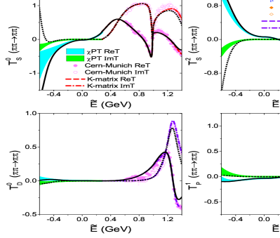
Figure 1: Fit of the $\pi\pi$ scattering amplitudes for Case B. Notice that $\tilde{E}=\rm{sgn}(s)\sqrt{s}$. The solid lines denote the real part of the amplitudes and the dotted, dashed, dash-dotted and dash-dot-dotted lines denote the imaginary part. The black lines are from our fit. The red lines are from a K-matrix fit DLY-MRP14 for the isospin-zero S-wave, and the violet lines are from CFDIV KPY for other waves. The borders of the cyan and green bands in the low-energy region are from $SU(2)$ and $SU(3)$ $\chi$PT, respectively. The CERN-Munich data are from Ref. CERN-Munich , and the OPE and OPE-DP data are from OPE1973 .

Here all the partial waves refer to Case B, in which the phase is cut off at $s=2.25$ GeV². The amplitudes from the other Cases are quite close to this one, except for the inelastic region and the distant l.h.c. ($\tilde{E}\leq-0.4$ GeV²). Our fit, both the real part (black solid line) and imaginary (black dotted line) part of the amplitudes shown in Fig. 1, is indistinguishable from that given by the K-Matrix DLY-MRP14 or CFDIV KPY . Note that the amplitudes given by Eq. (5) are exactly the same as those of the K-Matrix or CFDIV from $\pi\pi$ threshold to the inelastic threshold. This implies that the unitarity is respected. To test it quantitatively, we define

$$\mathcal{R}_{T^{I}_{J}} = \frac{1}{N}\sum_{n=1}^{N}\frac{|\Delta T^{I}_{J}(s_{n})|}{|T^{I}_{J}(s_{n})|}\;.$$ (16)

$\Delta T^{I}_{J}(s_{n})$ is the difference between our amplitude and that of Eq. (5). Here we choose $s_{n}=0.1-0.9$ GeV² for the S-waves, $s_{n}=0.1-0.8$ GeV² for the P-wave, and $s_{n}=0.1-1.0$ GeV² for the D-wave, with step of 0.1 GeV². These points are located between the $\pi\pi$ and the inelastic thresholds. From here on all the steps are chosen to be 0.1 GeV² (or 0.1 GeV for $\tilde{E}$). We find that $\mathcal{R}_{T^{0}_{S}}=0.1\%$, $\mathcal{R}_{T^{1}_{P}}=0.1\%$, $\mathcal{R}_{T^{2}_{S}}=1.4\%$, and $\mathcal{R}_{T^{0}_{D}}=1.4\%$. The violation of unitarity is rather small.

For $T^{I}_{J}(0)$, $\chi$PT could be used to fix it. The analytical $SU(3)$ 1-loop $\chi$PT amplitudes of each partial waves, are recalculated and given in Appendix. A. The low-energy constants are given by Bijnens:2014lea . Those of $SU(2)$ 2-loop $\chi$PT amplitudes are given by Bijnens:1997vq ; zhou04 and references therein. All the values of $T^{I}_{J}(0)$ in Tab. 1 are close to the prediction of $\chi$PT or our earlier analyses Dai:2017tew ; Dai:2017uao . In the isospin-zero S-wave, the magnitude of our $T^{0}_{0}(0)$ is a bit larger than that of $\chi$PT. This is consistent with what is known about this scattering length, where the one-loop $\chi$PT calculation gives a smaller result than what is obtained by dispersive methods, Roy equations or in experiment, see e.g. the review Bijnens:2014lea . A better comparison would be given with the 2-loop $\chi$PT amplitudes.

In the isospin-zero D-wave, the $T^{0}_{2}(0)$ varies more in the different Cases. The reason is that some fine-tuning is needed as the inelastic r.h.c. is difficult to be implemented well. The amplitudes given by Eq. (5) are much different from that of CFDIV in the inelastic region where the $f_{2}(1270)$ appears. Notice further that the value of $T^{0}_{D}(0)$ is very small, one order smaller than that of the other waves.

III.2 Pole locations and couplings

With these amplitudes given by a dispersion relation, the information of the poles can be extracted. The pole $s_{R}$ and its coupling/residue $g_{f\pi\pi}$ on the second Riemann sheet are defined as

$$T^{II}(s)=\frac{g_{f\pi\pi}^{2}}{s_{R}-s}\,.$$ (17)

Note that the continuation of the $T(s)$ amplitude to the second Riemann sheet is based on unitarity,

$$T^{II}(s+i\epsilon)=T^{I}(s-i\epsilon)=\frac{T^{I}(s+i\epsilon)}{S^{I}(s+i\epsilon)}\,.$$ (18)

The poles and couplings/residues for Cases A,B,C are given in Table 2.

State	Case	pole locations	$g_{f\pi\pi}=|g_{f\pi\pi}|e^{i\phi}$
		(MeV)	$~{}|g_{f\pi\pi}|~{}(GeV)~{}$	$~{}\phi~{}(^{\circ})~{}$
$\sigma/f_{0}(500)$	A	$432.5-i269.8$	$0.46$	$-77$
	B	$442.7-i270.5$	$0.48$	$-74$
	C	$438.2-i270.6$	$0.47$	$-75$
$f_{0}(980)$	A	$997.5-i19.0$	$0.25$	$-81$
	B	$997.6-i21.6$	$0.27$	$-83$
	C	$997.6-i20.5$	$0.26$	$-82$
$f_{2}(1270)$	A	$1260.9-i111.2$	$0.55$	$-10$
	B	$1294.1-i57.9$	$0.52$	$11$
	C	$1266.0-i99.5$	$0.54$	$-8$
$\rho(770)$	A	$761.1-i70.6$	$0.34$	$-12$
	B	$763.0-i73.3$	$0.35$	$-11$
	C	$761.3-i71.7$	$0.34$	$-12$
$2S~{}~{}v.s.$	A	$29.8$	$9.8\times 10^{-3}$	$90$
	B	$29.8$	$9.8\times 10^{-3}$	$90$
	C	$32.3$	$11.0\times 10^{-3}$	$90$

Table 2: The pole locations and residues given by our fits. The notation “$2S~{}~{}v.s.$” denotes the virtual state in the isospin-two $S$-wave.

All the poles and residues of the different Cases are close to each other, except for the pole location of the $f_{2}(1270)$. The reason is that the $f_{2}(1270)$ is located outside the elastic unitary cut of $T^{0}_{D}(s)$, while Eq. (11) only works in the elastic region. For this partial wave one needs a more dedicated method to study, including coupled-channel unitarity. For the poles of the $\sigma$, the differences between the different Cases is a also bit larger than those of other resonances such as the $\rho(770)$ and the $f_{0}(980)$. This is because the $\sigma$ is far away from the real axis. For the virtual state in the isospin-two S-wave, the poles and residues are a bit different from Cases A and B to Case C. This situation is comparable with that of $T^{2}_{S}(0)$, where in Cases A and B $T^{2}_{S}(0)$ is 0.055 and in Case C it is 0.060, respectively.

In addition, we also find that there exists a virtual state in the isospin-two S-wave very close to $s=0$ . According to Eq. (18), the virtual state a the zero of the S-matrix below the threshold. This zero equals to the intersection point between two lines: $T^{2}_{S}(s)$ and $i/2\rho(s)$. As shown in Fig. 2, the line of the $T^{2}_{S}(s)$ and the line of $i/2\rho(s)$ will always intersect with each other and the crossing point always lies in the energy region of [0,$s_{a}$], where $s_{a}$ is the Adler zero. This is the virtual state. Since the scattering length is negative and the Adler zero (only one) is below threshold, one would expect that the amplitude of $T^{2}_{S}(s)$, from $s=4M_{\pi}^{2}$ to $s=0$, will always cross the real axis of $s$ and arrive at the positive vertical axis. In all events, it will intersect with that of the $i/2\rho(s)$. Thus the existence of the virtual state is confirmed. This inference is model-independent, only the sign of the scattering length, the Adler zero, and analyticity are relevant.

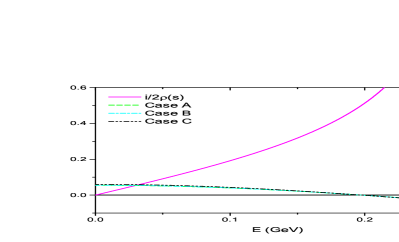
Figure 2: The lines of $T^{2}_{S}(s)$ for the different Cases and $i/2\rho(s)$. Note that all of them are real. The intersection point corresponds to the virtual state.

For a general discussion of the virtual state arising from a bare discrete state in the quantum mechanical scattering, we recommend readers to read Xiao2016 ; Xiao:2016mon and references therein. We suggest that the isospin-two S-wave amplitude could be checked in the future measurement of $\Lambda_{c}^{+}\to\Sigma^{-}\pi^{+}\pi^{+}$. Its branching ratio Ablikim:2017iqd is large enough.

The average values of the poles and residues of all the Cases define our central values. The deviations of the different Cases to the central values are used to estimate the uncertainties. The results are shown in Tab. 3.

State	pole locations	$g_{f\pi\pi}=|g_{f\pi\pi}|e^{i\phi}$
	(MeV)	$~{}|g_{f\pi\pi}|~{}(GeV)~{}$	$~{}\phi~{}(^{\circ})~{}$
$\sigma/f_{0}(500)$	$437.8(52)-i270.3(5)$	$0.47(1)$	$-75(2)$
$f_{0}(980)$	$997.6(1)-i20.3(13)$	$0.26(1)$	$-82(1)$
$f_{2}(1270)$	$1273.7(179)-i89.5(280)$	$0.53(2)$	$-3(12)$
$\rho(770)$	$761.8(11)-i71.9(14)$	$0.34(1)$	$-12(1)$
$2S~{}~{}v.s.$	$30.6(15)$	$10.2(7)\times 10^{-3}$	$90(0)$

Table 3: The pole locations and residues by taking the averages between Cases A, B and C as discussed in the text.

These are very similar from those of previous analyses caprini06 ; DLY-MRP14 ; PelaezPRL ; Rusetsky2011 ; PDG16 . The $f_{2}(1270)$ has a much larger uncertainty compared to the other resonances, just as discussed before. The residues of all resonances have roughly similar magnitude at the region [0.25,0.55] GeV, except for that of the virtual state in the isospin-two S-wave, which is much weaker. But their phases are quite different. The phases of $\rho(770)$ and $f_{2}(1270)$ are close to zero, while those of the $\sigma$ and $f_{0}(980)$ are close to $-90^{\circ}$, and the virtual state one is close to $90^{\circ}$. This may imply that $\rho(770)$ and $f_{2}(1270)$ are normal $\bar{q}q$ states but that the $\sigma$ and $f_{0}(980)$ have large molecular components.

III.3 The correlation between poles and cuts

It is interesting to find the correlation between the poles and cuts. We focus here on the isospin-zero S-wave and isospin-one P-wave, as the $f_{2}(1270)$ is far away from the l.h.c and the virtual state is too close to the l.h.c.. Also, the light scalars are more difficult to understand. All the fits of different Cases about these two partial waves are shown in Fig. 3.

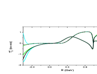
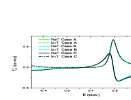
Figure 3: Comparison of different solutions of the $\pi\pi$ scattering amplitudes. The solid lines are the real part of the amplitudes and other lines are the imaginary part. The green lines are from Case A, the cyan lines are from Case B, and the black lines are from Case C. The red lines are from K-Matrix DLY-MRP14 for isospin 0 S-wave, and the violet lines are from CFDIV KPY for isospin 1 P-wave. Note that the lines of K-matrix and/or CDFIV are overlapped with our fits in the elastic region, or even a bit further in the inelastic region.

In our approach only unitarity is used to constrain the amplitudes, but the low-energy amplitudes are consistent with those of $\chi$PT. Only in Cases B and for the isospin-zero S-wave, the $T^{0}_{S}(s)$ amplitude is inconsistent with that of $\chi$PT at $\tilde{E}<-0.4$ GeV. This implies that unitarity has a strong constraint on the low-energy amplitudes below $\tilde{E}=0$. This could also be simply checked by using Eq. (16), with $\tilde{E}=-0.1$ to $-0.4$ GeV and $s_{n}=-\tilde{E}_{n}^{2}$. Here, $\Delta T^{I}_{J}(s_{n})$ is the difference between our amplitude and that of SU(2) $\chi$PT. Typically, in Case B, $\mathcal{R}^{L}_{T^{0}_{S}}=21\%$, $\mathcal{R}^{L}_{T^{1}_{P}}=16\%$, and they are quite close to those of other Cases. Note that the real parts of the amplitudes are more consistent with those of $\chi$PT, while the imaginary parts have a bit larger deviation (as is expected as imaginary parts start later in the chiral expansion).

To see the variation of the l.h.c. in the different solutions, we apply Eq. (19) on ${\rm Im}T^{I}_{J}(s_{n})$, with $\tilde{E}=-0.1$ to $-0.6$ GeV. Notice that at $\tilde{E}=0$ all of the l.h.c are zero and behave as $\sqrt{-s^{3}}$, this partly ensures the l.h.c to be consistent with that of $\chi$PT in the low-energy region. We fix the average value of all Cases as the central value, and calculate the relative deviation for each point. At last we avarage these relative deviations to estimate the variation of the cuts. The variation of cuts and poles are defined as

$$\mathcal{R}_{{\rm Im}T^{I}_{J}} = \frac{1}{N}\sum_{n=1}^{N}\frac{|\Delta{\rm Im}T^{I}_{J}(s_{n})|}{|{\rm Im}T^{I}_{J}(s_{n})|}\;,$$

$$\mathcal{R}_{pole} = \frac{|\Delta{\rm Re}\sqrt{s_{p}}|+|\Delta{\rm Im}\sqrt{s_{p}}|}{|\sqrt{s_{p}|}}\;,$$ (19)

with $s_{p}$ the pole on the second Riemann Sheet. Finally, we collect the uncertainties in Tab. 4. And we define the correlation between poles and cuts as

$$C_{pole}=\frac{\mathcal{R}_{pole}}{\mathcal{R}_{{\rm Im}T^{I}_{J}}}\,.$$ (20)

The simple meaning of the correlation $C_{pole}$ is to answer the following question: When the cut is changed by 100%, how much would the pole location be changed?

		Case A	Case B	Case C
l.h.c.	$\mathcal{R}_{{\rm Im_{L}}T^{0}_{S}}$	171%	126%	45%
	$C^{L}_{\sigma}$	2.01%	1.70%	2.87%
	$C^{L}_{f_{0}(980)}$	0.08%	0.10%	0.04%
	$\mathcal{R}_{{\rm Im_{L}}T^{1}_{P}}$	41%	20%	61%
	$C^{L}_{\rho}$	0.63%	1.75%	1.41%
r.h.c.	$\mathcal{R}_{{\rm Im_{R}}T^{0}_{S}}$	1.70%	0.64%	1.36%
	$C^{R}_{\sigma}$	387%	328%	189%
	$C^{R}_{f_{0}(980)}$	30%	142%	55%
	$\mathcal{R}_{{\rm Im_{R}}T^{1}_{P}}$	6.6%	10.0%	4.4%
	$C^{R}_{\rho}$	17.6%	6.4%	28.2%

Table 4: The correlation between l.h.c. and poles (represented by superscript ‘L’), and between r.h.c. and poles (represented by superscript ‘R’).

To test the correlation between poles and the r.h.c., we simply set $\varphi_{test}(s)=1.04\varphi(s)$, and check the variation of poles and cuts, respectively. The relative uncertainty of the r.h.c. is also estimated by Eq. (19), with $s_{n}=0.1-0.9$ GeV² for the isospin-zero S-wave and $s_{n}=0.1-0.8$ GeV² for the isospin-one P-wave. The relative uncertainty of the poles and the correlation are calculated in the same way as that of the l.h.c, see Eqs. (19,20).

From Tab. 4, we find that $C_{\sigma}^{R}$ is roughly two orders larger than that of $C_{\sigma}^{L}$, though $\sigma$ is rather close to the l.h.c.. Comparing to Ref. caprini06 , which has roughly 15% contribution from l.h.c, we have a rather smaller contribution from the l.h.c, caused by the constraint of unitarity on the l.h.c. . Also, $C_{f_{0}(980)}^{R}$ is roughly three orders larger than that of $C_{f_{0}(980)}^{L}$, and $C_{\rho(770)}^{R}$ is roughly one order larger than that of $C_{\rho(770)}^{L}$. These indicate that the correlation between the unitarity cut and the poles is much larger than that of the l.h.c. and poles. Note that in our case the l.h.c. is not arbitrary but correlated with the r.h.c., constrained by unitarity and analyticity, see Eq. (11). For each Case, $C_{\sigma}^{L}$ is larger than $C_{f_{0}(980)}^{L}$. This is not surprising as the $\sigma$ is much closer to the l.h.c. . Also, $C_{\sigma}^{R}$ is larger than $C_{f_{0}(980)}^{R}$. The reason is that the $\sigma$ is farther away from the real axis, the uncertainty of the pole is larger as the amplitude is continued from the physical region deeper into the complex-$s$ plane. It is interesting to see that in average $C_{\sigma}^{L}$ is roughly two times larger than $C_{\rho(770)}^{L}$. And for the distance between these poles and l.h.c (simply set $s=0$), $|s_{\sigma}|$ is one half of that of $|s_{\rho}|$, this tells us that the correlation between poles and l.h.c is inversely proportional to their distance. In contrast, $C_{\sigma}^{R}$ is roughly one order larger than $C_{\rho(770)}^{R}$. For the distance between these poles and r.h.c. (simply set $s={\rm Re}~{}s_{pole}$), $|{\rm Im}~{}s_{\sigma}|$ is two times larger than $|{\rm Im}~{}s_{\rho}|$, this tells us that the correlation between poles and r.h.c. is proportional to their distance. These conclusions are still kept when comparing the $\sigma$ and the $f_{0}(980)$.

IV Summary

We proposed a dispersive method to calculate the two-body scattering amplitude. It is based on the Omnès function of the phase, including that of the left hand cut and the right hand cut. The input of the r.h.c. is given by three kinds of parametrizations, and the l.h.c is solved by Eq. (11), with unitarity and analyticity respected. The pion-pion $IJ=00,02,11,20$ waves are fitted within our method and the poles and locations are extracted. They are stable except for that of the $f_{2}(1270)$, which lies in the inelastic region. The r.h.c. has much larger contribution to the poles comparing to that of the l.h.c.. This method could be useful for the studies of strong interactions in two-body scattering, and the $\pi\pi$ scattering amplitudes obtained here could be used for the future studies when one has $\pi\pi$ final state interactions, see e.g. AMP-FSI ; Dai:2012pb ; Gonzalez-Solis:2018xnw ; Ropertz:2018stk ; Cheng:2019hpq , and/or to multi-pions, see e.g.  Guo:2015zqa ; Dumm:2009va .

Appendix A Analytical amplitudes of partial waves within $\chi$PT

The analytical 1-loop amplitudes of these partial waves within of $SU(3)$ $\chi$PT are recalculated. For reader’s convenience, they are given below. We have the IJ=00 waves up to $\mathcal{O}(p^{4})$:

$$T^{(2)}_{0S}[s] = \frac{2s-M_{\pi}^{2}}{32\pi f_{\pi}^{2}}\;,$$ (A.1)

$$t_{0S,1}[s] = \frac{1}{3}(3s-4M_{\pi}^{2})A[M_{K}]+\frac{2}{3}(3s-4M_{\pi}^{2})A[M_{\pi}]+\frac{1}{6}M_{\pi}^{4}B[s,M_{\eta}]+\frac{3}{8}s^{2}B[s,M_{K}]$$ (A.2)

$$+\frac{1}{2}(2s-M_{\pi}^{2})^{2}B[s,M_{\pi}]+\frac{128\pi^{2}}{3}(-40M_{\pi}^{2}s+44M_{\pi}^{4}+11s^{2})L_{1}$$

$$+\frac{128\pi^{2}}{3}(-20M_{\pi}^{2}s+28M_{\pi}^{4}+7s^{2})L_{2}+\frac{64\pi^{2}}{3}(-40M_{\pi}^{2}s+44M_{\pi}^{4}+11s^{2})L_{3}$$

$$+256\pi^{2}M_{\pi}^{2}(s-3M_{\pi}^{2})(2L_{4}+L_{5})+1280\pi^{2}M_{\pi}^{4}(2L_{6}+L_{8})$$

$$-\frac{1}{9}(9sM_{K}^{2}-12M_{\pi}^{2}M_{K}^{2}+8M_{\pi}^{2}s-16M_{\pi}^{4}+2s^{2})\;,$$

$$t_{0S,2}[s] = -\left\{\frac{5}{12}H_{2}[4M_{\pi}^{2}-s,M_{K}]+2(\frac{1}{6}s-\frac{1}{3}M_{K}^{2}-\frac{1}{3}M_{\pi}^{2})H_{1}[4M_{\pi}^{2}-s,M_{K}]+\frac{10}{3}H_{2}[4M_{\pi}^{2}-s,M_{\pi}]\right.$$ (A.3)

$$+2(-\frac{2}{3}sM_{K}^{2}+\frac{4}{3}M_{K}^{2}M_{\pi}^{2})H_{0}[4M_{\pi}^{2}-s,M_{K}]+2(\frac{1}{3}s-\frac{16}{3}M_{\pi}^{2})H_{1}[4M_{\pi}^{2}-s,M_{\pi}]$$

$$\left.+2(-\frac{4}{3}sM_{\pi}^{2}+\frac{37}{6}M_{\pi}^{4})H_{0}[4M_{\pi}^{2}-s,M_{\pi}]+\frac{1}{9}M_{\pi}^{4}H_{0}[4M_{\pi}^{2}-s,M_{\eta}]\right\}\;,$$

$$T^{(4)}_{0S}[s] = \frac{1}{32\pi f_{\pi}^{2}}\frac{1}{16\pi^{2}f_{\pi}^{2}}\left(t_{0S,1}[s]+\frac{t_{0S,2}[s]}{s-4M_{\pi}^{2}}\right)\;.$$ (A.4)

Here the superscript of $T$ in the bracket means the chiral order, and subscripts represent for Isospin and spin, respectively. Note that for reader’s convenience we also give the analytical forms of the imaginary part (r.h.c.) of the amplitudes. The I=2 S wave is

$$T^{(2)}_{2S}[s] = -\frac{s-2M_{\pi}^{2}}{32\pi f_{\pi}^{2}}\;,$$ (A.5)

$$t_{2S,1}[s] = (\frac{2}{3}M_{\pi}^{2}-\frac{1}{2}s)A[M_{K}]+(\frac{4}{3}M_{\pi}^{2}-s)A[M_{\pi}]+\frac{1}{2}B[s,M_{\pi}](s-2M_{\pi}^{2})^{2}$$ (A.6)

$$+\frac{1}{18}(9sM_{K}^{2}-12M_{\pi}^{2}M_{K}^{2}-16M_{\pi}^{4}+2s^{2}+8M_{\pi}^{2}s)+\frac{256\pi^{2}}{3}(-2M_{\pi}^{2}s+4M_{\pi}^{4}+s^{2})L_{1}$$

$$+\frac{256\pi^{2}}{3}(-7M_{\pi}^{2}s+8M_{\pi}^{4}+2s^{2})L_{2}-128\pi^{2}M_{\pi}^{2}s(2L_{4}+L_{5})$$

$$+\frac{128\pi^{2}}{3}(-2M_{\pi}^{2}s+4M_{\pi}^{4}+s^{2})L_{3}+512\pi^{2}M_{\pi}^{4}(2L_{6}+L_{8})\;,$$

$$t_{2S,2}[s] = -2\left\{\frac{1}{12}H_{2}[4M_{\pi}^{2}-s,M_{K}]+(\frac{M_{K}^{2}}{6}+\frac{M_{\pi}^{2}}{6}-\frac{s}{12})H_{1}[4M_{\pi}^{2}-s,M_{K}]\right.$$ (A.7)

$$+(\frac{sM_{K}^{2}}{3}-\frac{2}{3}M_{\pi}^{2}M_{K}^{2})H_{0}[4M_{\pi}^{2}-s,M_{K}]+\frac{2}{3}H_{2}[4M_{\pi}^{2}-s,M_{\pi}]+(-\frac{M_{\pi}^{2}}{3}-\frac{s}{6})H_{1}[4M_{\pi}^{2}-s,M_{\pi}]$$

$$\left.+(\frac{2M_{\pi}^{2}s}{3}-\frac{5M_{\pi}^{4}}{6})H_{0}[4M_{\pi}^{2}-s,M_{\pi}]+\frac{M_{\pi}^{4}}{18}H_{0}[4M_{\pi}^{2}-s,M_{\eta}]\right\}\;,$$

$$T^{(4)}_{2S}[s] = \frac{1}{32\pi f_{\pi}^{2}}\frac{1}{16\pi^{2}f_{\pi}^{2}}\left(t_{2S,1}[s]+\frac{t_{2S,2}[s]}{s-4M_{\pi}^{2}}\right)\;.$$ (A.8)

The I=1 P wave is

$$T^{(2)}_{1P}[s] = \frac{s-4M_{\pi}^{2}}{96\pi f_{\pi}^{2}}\;,$$ (A.9)

$$t_{1P,1}[s] = \frac{1}{36}(s-4M_{\pi}^{2})\left\{3\left[2A[M_{K}]+4A[M_{\pi}]-2M_{K}^{2}+4M_{\pi}^{2}\left(128\pi^{2}(2L_{4}+L_{5})-1\right)\right.\right.$$ (A.10)

$$\left.\left.-256\pi^{2}s(2L_{1}-L_{2}+L_{3})+s\right]+B[s,M_{K}](s-4M_{K}^{2})+2B[s,M_{\pi}](s-4M_{\pi}^{2})\right\}\;,$$

$$t_{1P,2}[s] = -\left\{\frac{2}{3}H_{3}[4M_{\pi}^{2}-s,M_{K}]+\left(\frac{1}{6}(2s-4M_{K}^{2}-4M_{\pi}^{2})+\frac{1}{3}(s-4M_{\pi}^{2})\right)H_{2}[4M_{\pi}^{2}-s,M_{K}]\right.$$ (A.11)

$$+\left(\frac{1}{6}(-8sM_{K}^{2}+16M_{K}^{2}M_{\pi}^{2})+\frac{1}{12}(s-4M_{\pi}^{2})(2s-4M_{K}^{2}-4M_{\pi}^{2})\right)H_{1}[4M_{\pi}^{2}-s,M_{K}]$$

$$+\frac{1}{12}(s-4M_{\pi}^{2})(-8sM_{K}^{2}+16M_{K}^{2}M_{\pi}^{2})H_{0}[4M_{\pi}^{2}-s,M_{K}]+\frac{4}{3}H_{3}[4M_{\pi}^{2}-s,M_{\pi}]$$

$$+\left(\frac{2}{3}(s+2M_{\pi}^{2})+\frac{2}{3}(s-4M_{\pi}^{2})\right)H_{2}[4M_{\pi}^{2}-s,M_{\pi}]+\frac{2M_{\pi}^{4}}{9}H_{1}[4M_{\pi}^{2}-s,M_{\eta}]$$

$$+\left(-\frac{2}{3}(4sM_{\pi}^{2}+M_{\pi}^{4})+\frac{1}{3}(s+2M_{\pi}^{2})(s-4M_{\pi}^{2})\right)H_{1}[4M_{\pi}^{2}-s,M_{\pi}]$$

$$\left.-\frac{1}{3}(4sM_{\pi}^{2}+M_{\pi}^{4})(s-4M_{\pi}^{2})H_{0}[4M_{\pi}^{2}-s,M_{\pi}]+\frac{M_{\pi}^{4}}{9}(s-4m_{\pi}^{2})H_{0}[4M_{\pi}^{2}-s,M_{\eta}]\right\}\;,$$

$$T^{(4)}_{1P}[s] = \frac{1}{32\pi f_{\pi}^{2}}\frac{1}{16\pi^{2}f_{\pi}^{2}}\left(t_{1P,1}[s]+\frac{t_{1P,2}[s]}{(s-4M_{\pi}^{2})^{2}}\right)\;.$$ (A.12)

And the I=0 D wave is

$$T^{(2)}_{0D}[s] = 0\;,$$ (A.13)

$$t_{0D,1}[s] = \frac{1}{90}(s-4M_{\pi}^{2})^{2}\left(384\pi^{2}(2L_{1}+4L_{2}+L_{3})+1\right)\;,$$ (A.14)

$$t_{0D,2}[s] = -2\left\{\frac{5}{4}H_{4}[4M_{\pi}^{2}-s,M_{K}]+\left((-2M_{K}^{2}-2M_{\pi}^{2}+s)+\frac{5}{4}(s-4M_{\pi}^{2})\right)H_{3}[4M_{\pi}^{2}-s,M_{K}]\right.$$ (A.15)

$$+\left((8M_{\pi}^{2}M_{K}^{2}-4sM_{K}^{2})+(s-4M_{\pi}^{2})(-2M_{K}^{2}-2M_{\pi}^{2}+s)+\frac{5}{24}(s-4M_{\pi}^{2})^{2}\right)H_{2}[4M_{\pi}^{2}-s,M_{K}]$$

$$+\left((s-4M_{\pi}^{2})(8M_{\pi}^{2}M_{K}^{2}-4sM_{K}^{2})+(s-4M_{\pi}^{2})^{2}(-\frac{M_{K}^{2}}{3}-\frac{M_{\pi}^{2}}{3}+\frac{s}{6})\right)H_{1}[4M_{\pi}^{2}-s,M_{K}]$$

$$+(s-4M_{\pi}^{2})^{2}(\frac{4}{3}M_{\pi}^{2}M_{K}^{2}-\frac{2sM_{K}^{2}}{3})H_{0}[4M_{\pi}^{2}-s,M_{K}]+10H_{4}[4M_{\pi}^{2}-s,M_{\pi}]$$

$$+\left((2s-32M_{\pi}^{2})+10(s-4M_{\pi}^{2})\right)H_{3}[4M_{\pi}^{2}-s,M_{\pi}]$$

$$+\left((37M_{\pi}^{4}-8M_{\pi}^{2}s)+(s-4M_{\pi}^{2})(2s-32M_{\pi}^{2})+\frac{5}{3}(s-4M_{\pi}^{2})^{2}\right)H_{2}[4M_{\pi}^{2}-s,M_{\pi}]$$

$$+\left((s-4M_{\pi}^{2})(37M_{\pi}^{4}-8M_{\pi}^{2}s)+(s-4M_{\pi}^{2})^{2}(\frac{s}{3}-\frac{16M_{\pi}^{2}}{3})\right)H_{1}[4M_{\pi}^{2}-s,M_{\pi}]$$

$$+(s-4M_{\pi}^{2})^{2}(\frac{37M_{\pi}^{4}}{6}-\frac{4M_{\pi}^{2}s}{3})H_{0}[4M_{\pi}^{2}-s,M_{\pi}]+\frac{M_{\pi}^{4}}{3}H_{2}[4M_{\pi}^{2}-s,M_{\eta}]$$

$$\left.+(s-4M_{\pi}^{2})\frac{M_{\pi}^{4}}{3}H_{1}[4M_{\pi}^{2}-s,M_{\eta}]+\frac{M_{\pi}^{4}}{18}(s-4M_{\pi}^{2})^{2}H_{0}[4M_{\pi}^{2}-s,M_{\eta}]\right\}\;,$$

$$T^{(4)}_{0D}[s] = \frac{1}{32\pi f_{\pi}^{2}}\frac{1}{16\pi^{2}f_{\pi}^{2}}\left(t_{0D,1}[s]+\frac{t_{0D,2}[s]}{(s-4M_{\pi}^{2})^{3}}\right)\;.$$ (A.16)

It should be noted that in all these partial waves, $2L_{4}+L_{5}$ and $2L_{6}+L_{8}$ appear together DLY11 . The $A$, $B$, $H$ functions are given as below

$$A[m] = m^{2}\left(1-\ln\frac{m^{2}}{\mu^{2}}\right)\;,$$ (A.17)

$$B[s,m] = 2-\ln\frac{m^{2}}{\mu^{2}}-\rho(s,m)\ln\left(\frac{\rho(s,m)+1}{\rho(s,m)-1}\right)\;,$$ (A.18)

$$H_{0}[t,m] = -t\ln\frac{m^{2}}{\mu^{2}}+m^{2}\ln^{2}\left(\frac{\rho(t,m)+1}{\rho(t,m)-1}\right)-t\rho(t,m)\ln\left(\frac{\rho(t,m)+1}{\rho(t,m)-1}\right)+3t\;,$$ (A.19)

$$H_{1}[t,m] = \frac{1}{4}t^{2}\left(5-2\ln\frac{m^{2}}{\mu^{2}}\right)-m^{2}t+m^{4}\ln^{2}\left(\frac{\rho(t,m)+1}{\rho(t,m)-1}\right)-\frac{1}{2}t(t-2m^{2})\rho(t,m)\ln\left(\frac{\rho(t,m)+1}{\rho(t,m)-1}\right)\;,$$ (A.20)

$$H_{2}[t,m] = \frac{1}{9}t^{3}\left(7-3\ln\frac{m^{2}}{\mu^{2}}\right)-\frac{1}{6}m^{2}t^{2}-\frac{1}{3}t\rho(t,m)(-tm^{2}-6m^{4}+t^{2})\ln\left(\frac{\rho(t,m)+1}{\rho(t,m)-1}\right)$$ (A.21)

$$-2m^{4}t+2m^{6}\ln^{2}\left(\frac{\rho(t,m)+1}{\rho(t,m)-1}\right)\;,$$

$$H_{3}[t,m] = -\frac{1}{12}t\rho(t,m)(-2t^{2}m^{2}-10tm^{4}-60m^{6}+3t^{3})\ln\left(\frac{\rho(t,m)+1}{\rho(t,m)-1}\right)$$ (A.22)

$$+\frac{1}{16}t^{4}\left(9-4\ln\frac{m^{2}}{\mu^{2}}\right)-\frac{1}{18}t^{3}m^{2}-\frac{5}{12}t^{2}m^{4}-5tm^{6}+5m^{8}\ln^{2}\left(\frac{\rho(t,m)+1}{\rho(t,m)-1}\right)\;,$$

$$H_{4}[t,m] = \frac{1}{25}t^{5}\left(11-5\ln\frac{m^{2}}{\mu^{2}}\right)-\frac{1}{40}t^{4}m^{2}-\frac{7}{45}t^{3}m^{4}-\frac{7}{6}t^{2}m^{6}-14tm^{8}+14m^{10}\ln^{2}\left(\frac{\rho(t,m)+1}{\rho(t,m)-1}\right)$$ (A.23)

$$-\frac{1}{30}t\rho(t,m)(-3t^{3}m^{2}-14t^{2}m^{4}-70tm^{6}-420m^{8}+6t^{4})\ln\left(\frac{\rho(t,m)+1}{\rho(t,m)-1}\right)\;,$$

with $\rho(t,m)=\sqrt{1-4m^{2}/t}$. Notice that our amplitudes are calculated in the formalism of $\overline{MS}$, while that of Gasser1984 ; Pelaez02 ; Guo2011 is done in $\overline{MS}-1$. The relation between our LECs ($L_{i}$) and that of the latter one ($\tilde{L}_{i}$) is $\tilde{L}_{i}=L_{i}+\frac{\Gamma_{i}}{32\pi^{2}}$.

References

• (1) M.R. Pennington, AIP Conf. Proc. 1257 27, (2010), arXiv: 1003.2549 [hep-ph].
• (2) R.J. Jaffe, Phys. Rev. D15, 267 (1977), Phys. Rept. 409, 1 (2005).
• (3) U.-G. Meißner, Comments Nucl. Part. Phys.  20, 119 (1991).
• (4) G. Colangelo, M. Hoferichter and P. Stoffer, JHEP 1902, 006 (2019), arXiv: 1810.00007 [hep-ph].
• (5) I. Danilkin and M. Vanderhaeghen, Phys. Lett. B 789, 366 (2019) arXiv: 1810.03669 [hep-ph].
• (6) X.W. Kang, B. Kubis, C. Hanhart and U.G. Meissner, Phys. Rev. D89, 053015 (2014, arXiv: 1312.1193 [hep-ph].
• (7) L.Y. Dai and M.R. Pennington, Phys. Lett. B736 11 (2014), arXiv: 1403.7514 [hep-ph]; Phys. Rev. D 90, 036004 (2014), arXiv: 1404.7524 [hep-ph].
• (8) Yun-Hua Chen, Johanna T. Daub, Feng-Kun Guo, Bastian Kubis, Ulf-G. Meißner and Bing-Song Zou, Phys. Rev. D93, 034030 (2015), arXiv: 1512.03583 [hep-ph].
• (9) C. Hanhart, S. Holz, B. Kubis, A. Kupść, A. Wirzba and C. W. Xiao, Eur. Phys. J. C 77, no. 2, 98 (2017), Erratum: [Eur. Phys. J. C 78, no. 6, 450 (2018)], arXiv: 1611.09359 [hep-ph].
• (10) Z.G. Xiao and H.Q. Zheng, Nucl. Phys. A695, 273 (2001), arXiv: 0011260 [hep-ph].
• (11) G. Colangelo, J. Gasser and H. Leutwyler, Nucl. Phys. B603, 125 (2001), arXiv: 0103088 [hep-ph].
• (12) Z.Y. Zhou, G. Y. Qin, P. Zhang, Z. G. Xiao, H. Q. Zheng, and N. Wu, JHEP 0502 043 (2005), arXiv: 0406271 [hep-ph].
• (13) S. Descotes-Genon, B. Moussallam, Eur. Phys. J. C48, 553 (2006), arxiv: [hep-ph/0607133].
• (14) I. Caprini, G. Colangelo and H. Leutwyler, Phys. Rev. Lett. 96, 132001 (2006), arXiv: 0512364 [hep-ph].
• (15) R. García-Martín, R. Kamiński, J. R. Peláez, and J. Ruiz de Elvira, Phys. Rev. Lett. 107, 072001 (2011), arXiv: 1107.1635 [hep-ph];
• (16) L. Y. Dai and U.-G. Meißner, Phys. Lett. B 783, 294 (2018) arXiv: 1706.10123 [hep-ph]; L. Y. Dai, X. W. Kang and U. G. Meißner, Phys. Rev. D 98, 074033 (2018), arXiv: 1808.05057 [hep-ph].
• (17) L. Y. Dai, X. W. Kang, U.-G. Meißner, X. Y. Song and D. L. Yao, Phys. Rev. D 97, 036012 (2018), arXiv: 1712.02119 [hep-ph].
• (18) R. García- Martín, R. Kamiński, J. R. Peláez, J. Ruiz de Elvira, and F. J. Ynduráin, Phys. Rev. D 83, 074004 (2011), arXiv: 1102.2183 [hep-ph].
• (19) B. Hyams, et al., Nucl. Phys. B64 134 (1973); G. Grayer, et al., Nucl. Phys. B75, 189 (1974); B. Hyams, et al., Nucl. Phys. B100, 205 (1975).
• (20) N. B. Durusoy, M. Baubillier, R. George, M. Goldberg and A. M. Touchard, Phys. Lett. B45, (1973) 517;
• (21) J. Bijnens and G. Ecker, Ann. Rev. Nucl. Part. Sci.  64, 149 (2014) arXiv:1405.6488 [hep-ph].
• (22) J. Bijnens, G. Colangelo, G. Ecker, J. Gasser and M. E. Sainio, Nucl. Phys. B 508, 263 (1997), Erratum: [Nucl. Phys. B 517, 639 (1998)], arXiv:hep-ph/9707291.
• (23) Q. Ang, Z. Xiao, H. Zheng and X. C. Song, Commun. Theor. Phys.  36, 563 (2001), arXiv:hep-ph/0109012.
• (24) S. R. Beane et al. [NPLQCD Collaboration], Phys. Rev. D 85, 034505 (2012), arXiv: 1107.5023 [hep-lat].
• (25) Z. Fu, Phys. Rev. D 87, no. 7, 074501 (2013), arXiv: 1303.0517 [hep-lat].
• (26) C. Helmes et al. [ETM Collaboration], JHEP 1509, 109 (2015), arXiv: 1506.00408 [hep-lat].
• (27) G. Colangelo, J. Gasser and H. Leutwyler, Phys. Lett. B 488, 261 (2000), arXiv:hep-ph/0007112.
• (28) Z.G. Xiao and Z.Y. Zhou, Phys. Rev. D94, (2016) 076006, arXiv: 1608.00468 [hep-ph].
• (29) Z. Xiao and Z. Y. Zhou, J. Math. Phys.  58, 072102 (2017), arXiv: 1610.07460 [hep-ph].
• (30) M. Ablikim et al. [BESIII Collaboration], Phys. Lett. B 772, 388 (2017), arXiv: 1705.11109 [hep-ph].
• (31) M. Döring, Ulf-G. Meißner, E. Oset, A. Rusetsky, Eur. Phys. J. A47, 139 (2011), arXiv: 1107.3988 [hep-lat]; Eur. Phys. J. A48, 114 (2012), arXiv: 1205.4838 [hep-lat].
• (32) C. Patrignani et al., [PDG], Chin. Phys. C40, 100001 (2016).
• (33) K.L. Au, D. Morgan and M.R. Pennington, Phys. Rev. D 35, 1633 (1987); D. Morgan and M.R. Pennington, Phys. Rev. D 48, 1185 (1993).
• (34) L. Y. Dai, M. Shi, G. Y. Tang and H. Q. Zheng, Phys. Rev. D 92, 014020 (2015), arXiv: 1206.6911 [hep-ph].
• (35) S. Gonzalez-Solis and E. Passemar, Eur. Phys. J. C 78, 758 (2018), arXiv: 1807.04313 [hep-ph].
• (36) S. Ropertz, C. Hanhart and B. Kubis, Eur. Phys. J. C 78, no. 12, 1000 (2018) arXiv: 1809.06867 [hep-ph].
• (37) S. Cheng, arXiv: 1901.06071 [hep-ph].
• (38) P. Guo, I. V. Danilkin, D. Schott, C. Fernandez-Ramirez, V. Mathieu and A. P. Szczepaniak, Phys. Rev. D 92, 054016 (2015), arXiv: 1505.01715 [hep-ph].
• (39) D. G. Dumm, P. Roig, A. Pich and J. Portoles, Phys. Lett. B 685, 158 (2010), arXiv: 0911.4436 [hep-ph].
• (40) L.Y. Dai, X.G. Wang and H.Q. Zheng, Commun. Theor. Phys. 57, 841 (2012), arXiv: 1108.1451 [hep-ph]; Commun. Theor. Phys. 58, 410 (2012), arXiv: 1206.5481 [hep-ph].
• (41) J. Gasser, H. Leutwyler, Ann. Phys. (NY) 158, 142 (1984).
• (42) A. Gomez Nicola, J. R. Pelaez, Phys. Rev. D 65, 054009 (2002). arXiv: 0109056 [hep-ph].
• (43) Z.H. Guo and J. A. Oller, Phys. Rev. D 84, 034005 (2011), arXiv: 1104.2849 [hep-ph].