Evolution of wave pulses in fully nonlinear shallow-water theory

Abstract

We consider evolution of wave pulses with formation of dispersive shock waves in framework of fully nonlinear shallow-water equations. Situations of initial elevations or initial dips on the water surface are treated and motion of the dispersive shock edges is studied within the Whitham theory of modulations. Simple analytical formulas are obtained for asymptotic stage of evolution of initially localized pulses. Analytical results are confirmed by exact numerical solutions of the fully nonlinear shallow-water equations.

I Introduction

Although the shallow-water theory is a classical subject of investigations with a huge number of papers devoted to it, it still remains very active field of research with many important applications (see, e.g., books and review articles debnath-94 ; johnson-97 ; aosl-07 ; ma-10 ; paldor-15 ; apm-2018 and references therein). Even in its simplest formulation in one-dimensional geometry, when one neglects dissipation effects and non-uniformity of the basin’s bottom, the interplay of nonlinearity and dispersion effects leads to quite complicated wave patterns and many approximate models were suggested for their description. For example, if the nonlinearity and dispersion effects are taken into account in the lowest approximation and one considers a one-directional propagation of the wave, then its dynamics is governed by the celebrated Korteweg-de Vries (KdV) equation kdv-1895 and one can distinguish the following typical wave patterns. (i) Transition between two different values of water elevation is accomplished by an undular bore bl-54 which theory in the framework of the Whitham theory of modulations whitham-65 ; whitham-74 was developed by Gurevich and Pitaevskii gp-73 . (ii) A localized pulse of positive elevation develops a transitory dispersive shock wave (DSW) Gur91 ; Gur92 ; Kry92 ; wright ; tian which evolves eventually into a sequence of bright solitons karpman-67 accompanied by some amount of linear radiation. (iii) If the initial pulse forms a dip in the water surface, then it cannot evolve into a sequence of bright solitons propagating along water surface and evolves instead into a nonlinear wave packet consisting of several regions with different characteristic features of their behavior an-73 ; zm-76 ; as-77 ; Seg81 ; ek-93 ; dvz-94 ; ekv-01 ; cg-09 ; cg-10 (application of Whitham theory to this problem has been recently reconsidered in Ref. ikp-18 ). These patterns agree qualitatively with observed phenomena but comparison with experiments (see, e.g., hs-78 ; clauss-99 ; carmo-13 ; tkco-16 ) shows that the KdV approximation is not good enough for quantitative description and one needs to go beyond KdV approximation.

In KdV theory, there are two small parameters which characterize the nonlinear and dispersion effects, respectively. In typical experimental situations, the amplitude of the wave is not very small compared with the water depth, so the corresponding nonlinearity parameter often cannot be considered as small. Therefore considerable efforts were directed to the derivation of the corresponding wave equations where only small dispersive effects are assumed. One of the most popular models was first suggested and studied in much detail by Serre serre-53 and later the same equations were derived in Refs. sg-69 ; gn-76 what has lead to different names attached to this system in literature. We shall call them, as some other authors, the “Serre equations” after their first discoverer and investigator.

Serre equations have nice periodic and soliton solutions, so the Whitham theory of modulations can be formulated in framework of the standard approach whitham-65 ; whitham-74 . However, on the contrary to the KdV equation theory, in the Serre equation case the Whitham modulation equations cannot be transformed to the diagonal Riemann form and lack of Riemann invariants hinders applications of the Whitham modulation theory to description of waves obeying the Serre equations. In spite of that, some important consequences of the Whitham theory can be derived without knowledge of the Riemann invariants. In particular, a smooth part of the wave is typically described by two equations of the dispersionless approximation which admits transformation to the Riemann diagonal form, and the same situation takes place in the Serre equations theory. Hence, if a one-directional (simple wave) propagation is considered, then one of the Riemann invariants is constant. If this simple wave breaks with formation of the DSW, then, as was first supposed by Gurevich and Meshcherkin gm-84 , the flows at both edges of the DSW have the same values of the corresponding dispersionless Riemann invariant. As Gurevich and Meshcherkin remarked, this rule “plays the same role in dispersive hydrodynamics as the shock Rankine-Hugoniot condition in ordinary dissipative hydrodynamics” and it “does not depend on the nature of dispersive effects”. This Gurevich-Meshcherkin conjecture and its generalizations play an important role in the general theory of DSWs.

Specific dispersive properties of the system under consideration enter into the general theory in the form of Whitham’s “number of waves” conservation law whitham-65 ; whitham-74

$$\frac{\partial k}{\partial t}+\frac{\partial\omega(k)}{\partial x}=0,$$ (1)

where $k=2\pi/L$ is the wave number, $L$ is the wavelength of the nonlinear periodic wave, $\omega=kV$, $V$ being the phase velocity of the periodic wave. This equation is valid along the whole DSW and in the limit of vanishing wave amplitude the function $\omega(k)$ becomes a dispersion law of linear waves known from a linear theory. Naturally, besides wave number $k$, it depends also on the parameters of the background smooth flow, and evolution of all these parameters, including value of $k$ at the corresponding edge of the DSW, obeys the limiting form of the Whitham modulation equations. A profound observation was made by El El05 who noticed that at the boundary with the simple wave these parameters depend on a single parameter, hence Eq. (1) transforms to the ordinary differential equation which can be integrated and the value of the corresponding integration constant can be determined from the Gurevich-Meshcherkin closure condition. Thus, one can calculate the wave number at the small-amplitude edge of the DSW what is enough for finding its speed equal to the corresponding group velocity $v_{g}(k)=d\omega/dk$ equal to the velocity of propagation of the small-amplitude edge in evolution of bores emerging from initial step-like discontinuities.

The situation at the opposite soliton edge of the DSW is more intricate. The number of waves conservation law (1) loses here its meaning since both $k$ and $\omega$ vanish at this edge. Nevertheless, one can include into consideration the old common wisdom (see, e.g., ai-77 ; dkn-03 ) that a soliton propagates with the same velocity as its tails and if these tails decay exponentially $\propto\exp[-\widetilde{k}|x-V_{s}t|]$, then such a small-amplitude tail obeys the same linear approximation of the evolution equations, as a linear propagating wave, so that the exponential law can be obtained from a harmonic linear wave $\propto\exp[i(kx-\omega(k)t]$ by means of a simple substitution

$$V_{s}={\widetilde{\omega}(\widetilde{k})}/{\widetilde{k}},\qquad\widetilde{\omega}(\widetilde{k})\equiv-i\omega(i\widetilde{k}),$$ (2)

where $\widetilde{k}$ has a meaning of the inverse half-width of the soliton and $V_{s}$ is its velocity. However, $\widetilde{k}$ and $\widetilde{\omega}$ do not satisfy the “solitonic counterpart”

$$\frac{\partial\widetilde{k}}{\partial t}+\frac{\partial\widetilde{\omega}(\widetilde{k})}{\partial x}=0$$ (3)

of Eq. (1) even at the soliton edge of the DSW. To overcome this difficulty, El studied the soliton limit of Eq. (1) and found that under certain assumptions this limiting equation can also be transformed to the ordinary differential equation which can be again solved with the boundary condition determined from the Gurevich-Meshcherkin condition. Thus, the inverse half-width $\widetilde{k}$ at the soliton edge is found as well as the soliton velocity provided the parameters of the smooth solution at this edge are already known. Since the parameters of the smooth flows at both edges of the DSW are known in problems related with self-similar evolution of step-like initial discontinuities, this El’s scheme El05 works perfectly well in considerations of this type of problems and it has found a number of applications egkkk-07 ; ep-11 ; hoefer-14 ; hek-17 including the theory of undular bores in the Serre equations theory egs-06 . It is worth noticing that El’s method can be formulated effectively as an “extrapolation” of a solution of the limiting Whitham equations from one edge of the DSW to the opposite edge where this limiting form is not correct anymore. This simplified formulation provides some advantages in generalizations of the El method, although one should remember that the statements of the original formulation are strict in framework of the Whitham method and of such additional assumptions as, e.g., the validity of the Gurevich-Meshcherkin closure condition.

The integrals of modulation equations along the limiting characteristics of the DSW edges hold not only for the initial step-like distributions. They remain correct in any situations with breaking of simple waves and this observation allowed El and coauthors in Ref. egs-08 to develop the method for finding the number of solitons evolved from initial conditions admitting the final state of the pulse evolution in the form of solitons trains. The distribution function of solitons amplitudes was also found. This method was applied in Ref. egs-08 to investigation of asymptotic stage of evolution of positive pulses for the Serre system. This generalizes the Karpman formula karpman-67 and its analogues for other integrable equations (see, e.g., kku-02 ; kku-03 ) to non-integrable situations. However, intermediate stages of evolution often observed in actual experiments with formation of DSWs remained inaccessible for analytical description.

To go beyond the initial step-like type of problem of Ref. egs-06 or asymptotic limit of Ref. egs-08 , one has to use some additional information about properties of the Whitham modulation equations at the edges of DSWs. In particular, it is well known that the characteristic velocities of the Whitham system reduce at the DSW edges, first, to the smooth flow velocity at the edge and, second, either to the group velocity at the small-amplitude edge or to the soliton velocity at the soliton edge. Besides that, we often know also the simple-wave solution adjacent to the DSW. As was shown in Ref. gkm-89 for the KdV equation case, this information together with the known limiting expressions for Whitham equation allows one to find the law of motion of the corresponding small-amplitude edge for the general form of the simple-wave initial condition. This idea was used also in Ref. kamch-18 for finding the low of motion of the soliton edge of the DSW in the theory of another integrable Gross-Pitaevskii (or NLS) equation. To extend this method to non-integrable equations, we can resort to El’s method of calculation of the characteristic velocities and to combine it with well-known hodograph form of the Whitham equations (see, e.g., kamch-2000 ). As was shown in Ref. kamch-19 , such an approach permits one to find some most important properties of pulse evolution in simple enough analytic form and the analytical results were confirmed by comparison with exact numerical solutions of such prototypical equations as generalized KdV equation and generalized NLS equation. In this paper, we shall apply the method of Ref. kamch-19 to investigation of evolution of initial simple-wave pulses in the Serre equations theory.

II Serre equations, their solutions and dispersionless limit

We consider the Serre equations in standard non-dimensional form

$$\begin{split}&h_{t}+(hu)_{x}=0,\\ &u_{t}+uu_{x}+h_{x}=\frac{1}{3h}\left[h^{3}(u_{xt}+uu_{xx}-(u_{x})^{2})\right]_{x},\end{split}$$ (4)

where $h$ is the total depth and $u$ is the horizontal velocity averaged over the water layer depth. Looking for the travelling wave solution in the form $h=h(\xi)$, $u=u(\xi)$, $(\xi=x-Vt)$, we find (see, e.g., egs-06 ):

$$\begin{split}&h(\xi)=h_{3}-(h_{3}-h_{2})\mathrm{sn}^{2}\left[\frac{1}{2}\sqrt{\frac{3(h_{3}-h_{1})}{h_{1}h_{2}h_{3}}}\,\xi,m\right],\\ &u(\xi)=V-\frac{h_{1}h_{2}h_{3}}{h(\xi)},\qquad 0<h_{1}\leq h_{2}\leq h_{3},\end{split}$$ (5)

where

$$m=\frac{h_{3}-h_{2}}{h_{3}-h_{1}}$$ (6)

and $h(\xi)$ oscillates in the interval

$$h_{2}\leq h(\xi)\leq h_{3}.$$ (7)

Thus, the periodic solution of the Serre equations is parameterized by four constant parameters $h_{1},h_{2},h_{3},V$ in terms of which all other characteristic variabled can be expressed. In particular, the wavelength is given by the formula

$$L=4\sqrt{\frac{h_{1}h_{2}h_{3}}{3(h_{3}-h_{1})}}K(m),$$ (8)

where $K(m)$ is the elliptic integral of the first kind.

According to the Gurevich-Pitaevskii approach gp-73 , a DSW can be approximated by a modulated periodic solution with slowly varying parameters $h_{1},h_{2},h_{3},V$ which change little in one wavelength $L$. In typical situations, at one its edge, where $h_{3}-h_{2}\ll h_{2}$, the DSW degenerates into the harmonic linear wave

$$\begin{split}h&\approx h_{2}+\frac{1}{2}(h_{3}-h_{2})\cos\left[\frac{1}{h_{2}}\sqrt{3\left(\frac{h_{2}}{h_{1}}-1\right)}(x-Vt)\right],\\ u&\approx V-\sqrt{h_{1}}+\frac{\sqrt{h_{1}}}{2}\left(\frac{h_{3}}{h_{2}}-1\right)\\ &\times\cos\left[\frac{1}{h_{2}}\sqrt{3\left(\frac{h_{2}}{h_{1}}-1\right)}(x-Vt)\right]\end{split}$$

If we denote the background depth $h_{2}=h_{0}$, the background flow velocity $V-\sqrt{h_{1}}\equiv\omega/k-\sqrt{h_{1}}=u_{0}$, and the wavenumber of the harmonic wave

$$k=\frac{1}{h_{2}}\sqrt{3\left(\frac{h_{2}}{h_{1}}-1\right)},$$

then we get at once the well-known dispersion law

$$\omega(k)=u_{0}k+k\sqrt{\frac{h_{0}}{1+h_{0}^{2}k^{2}/3}}$$ (9)

obtained from the Serre equations linearized with respect to the background state of water flow.

At the opposite edge for $h_{2}\to h_{1}$ the DSW transforms into a train of solitons where the single soliton solution has the form

$$h=h_{1}+\frac{h_{3}-h_{1}}{\cosh^{2}\left[\frac{1}{2h_{1}}\sqrt{3\left(1-\frac{h_{1}}{h_{3}}\right)}(x-V_{s}t)\right]}.$$ (10)

This is a bright soliton propagating along uniform water depth $h_{1}=h_{0}$ and background flow with velocity $u_{0}=V_{s}-\sqrt{h_{3}}$. If we introduce the inverse half-width of the soliton

$$\widetilde{k}=\frac{1}{h_{0}}\sqrt{3\left(1-\frac{h_{0}}{h_{3}}\right)},$$ (11)

then the soliton velocity can be represented as

$$V_{s}=\frac{\widetilde{\omega}}{\widetilde{k}},\qquad\widetilde{\omega}=u_{0}\widetilde{k}+\widetilde{k}\sqrt{\frac{h_{0}}{1-h_{0}^{2}\widetilde{k}^{2}/3}},$$ (12)

where $\widetilde{\omega}$ is related with the linear dispersion law (9) by the identity (2). If the soliton propagates along a quiescent background ($u_{0}=0$), then its amplitude is related with its velocity by the equation

$$a\equiv h_{3}-h_{1}=V_{s}^{2}-h_{1}.$$ (13)

In a modulated wave the parameters $h_{1},h_{2},h_{3},V$ become slow functions of $x$ and $t$ and their evolution is governed by the Whitham modulation equations which can be obtained by averaging the conservation laws whitham-65 . Although Eq. (3) is not fulfilled, generally speaking, even along the soliton edge of DSW, one can check kamch-19 that this equation is correct for integrable KdV and NLS evolution equations for situations, when DSW propagates into “still” medium. In completely integrable situations of KdV and NLS equations type where the Whitham equations can be cast to the Riemann diagonal form, such situations were called in Ref. gkm-89 as “quasi-simple waves” with two Riemann invariants constant. In non-integrable case the Riemann invariants of Whitham equations do not exist anymore, but one can generalize the notion of quasi-simple wave as such a wave which formal dispersionless representation is given by a multi-valued solution with two dispersionless Riemann invariants constant (see Ref. kamch-19 ). Then we can assume that Eq. (3) is fulfilled along the soliton edge and in its vicinity. Along this edge Eq. (3) reduces to the ordinary differential equation and its extrapolation to the whole DSW yields with account of appropriate boundary condition the value of $\widetilde{k}$ at the soliton edge. For the initial step-like pulses, this procedure is equivalent to the El method El05 and the advantage of formulated here interpretation is that it can be applied to arbitrary simple-wave initial pulses.

In dispersionless limit, the Serre equations reduce to the shallow water equations

$$\begin{split}h_{t}+(hu)_{x}=0,\qquad u_{t}+uu_{x}+h_{x}=0,\end{split}$$ (14)

which describe evolution of a smooth pulses outside the DSW. After introduction of the Riemann invariants

$$r_{+}=\frac{u}{2}+\sqrt{h},\qquad r_{-}=\frac{u}{2}-\sqrt{h},$$ (15)

Eqs. (14) can be written in the form

$$\begin{split}&\frac{\partial r_{+}}{\partial t}+v_{+}(r_{+},r_{-})\frac{\partial r_{+}}{\partial x}=0,\\ &\frac{\partial r_{-}}{\partial t}+v_{-}(r_{+},r_{-})\frac{\partial r_{-}}{\partial x}=0,\end{split}$$ (16)

where

$$\begin{split}&v_{+}(r_{+},r_{-})=\frac{1}{2}(3r_{+}+r_{-}),\\ &v_{-}(r_{+},r_{-})=\frac{1}{2}(r_{+}+3r_{-})\end{split}$$ (17)

It is well known that any localized initial pulse with initial distributions of $h(x,0)$, $u(x,0)$ different from some constant values $h_{0},u_{0}$ on a finite interval of $x$ evolves eventually into two separate pulses propagating in opposite directions. For example, formation of such pulses from an initial hump of elevation $h(x,0)$ has been recently considered in another physical (nonlinear optics) context in Ref. ikp-19 where the non-dispersive evolution is also governed by the system (14). These two pulses are called simple-wave solutions in which one of the Riemann invariants $r_{\pm}$ is constant. In this paper, we suppose that the initial state belongs to such a class of simple waves. To be definite, we assume that $r_{-}=u/2-\sqrt{h}=-\sqrt{h_{0}}=\mathrm{const}$, that is we consider the right-propagating wave. If we denote $\sqrt{h}=c$, $\sqrt{h_{0}}=c_{0}$, then we get

$$u=2(c-c_{0}),\quad r_{+}=2c-c_{0},\quad v_{+}=3c-2c_{0}.$$ (18)

The second equation (16) is satisfied identically by virtue of our assumption and the first one takes the form

$$c_{t}+(3c-2c_{0})c_{x}=0$$ (19)

with well-known solution

$$x-(3c-2c_{0})t=\overline{x}(c),$$ (20)

where $\overline{x}(c)$ is the function inverse to the initial distribution of the local sound velocity $c(x,0)$.

Now we can proceed to discussion of DSWs formed after wave breaking of such pulses.

III Positive pulse

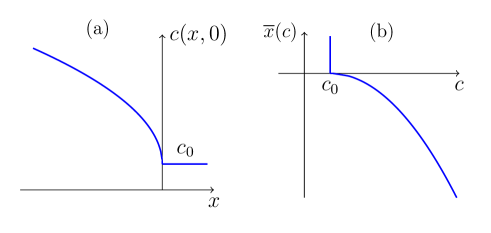
Figure 1: (a) The initial distribution of the local sound velocity $c(x,0)$ in a monotonous positive pulse. (b) Inverse function $\overline{x}(c)$.

At first we shall consider a monotonous initial distribution

$$c(x,0)=\begin{cases}c_{0}+\widetilde{c}(x)&\mbox{if}\quad x<0,\\ c_{0}&\mbox{if}\quad x\geq 0,\end{cases}$$ (21)

where $\widetilde{c}(x)$ monotonously increases with decrease of $x$; see Fig. 1(a). In Serre equations theory, the dispersion and nonlinearity lead to formation of wave patterns qualitatively similar to those in the KdV equation theory. Hence, we can see at once that if the initial distribution of the local sound velocity $c$ has the form of a hump (“positive pulse”), then the wave breaking occurs at the front of the pulse with formation of solitons at the front edge of the DSW and with small-amplitude edge at the boundary with the smooth part of the pulse described by Eq. (20) (rear edge of the DSW). Therefore, we can find by the method of Ref. kamch-19 the law of motion of the rear small-amplitude edge of the DSW.

To this end, we assume that in vicinity of this edge Eq. (1) must be satisfied where $k=k(c)$ is an unknown function to be found, and $u=2(c-c_{0})$ (see Eq. (18)). It is convenient to represent the function $k=k(c)$ in another form with the use of the dispersion relation (9),

$$\omega(k)=uk+kc(1+c^{4}k^{2}/3)^{-1/2}=k[u+c\alpha(k)],$$ (22)

that is the function

$$\alpha(k)=(1+c^{4}k^{2}/3)^{-1/2},\qquad(0<\alpha<1),$$

measures deviation of the dispersion law from the linear non-dispersive law $\omega=(u+c)k$, and then we have

$$k(c)=\frac{\sqrt{3}}{c^{2}}\sqrt{\frac{1}{\alpha^{2}}-1},$$ (23)

where $\alpha=\alpha(c)$ is an unknown yet function. In the simple wave solution the Riemann invariant $r_{+}=r_{+}(c)$ and $v_{+}=u+c$ are functions of $c$ only, so that the first equation (16) can be cast to the form

$$\frac{\partial c}{\partial t}+(u+c)\frac{\partial c}{\partial x}=0.$$ (24)

Substitution of Eqs. (22)-(24) into Eq. (1) yields after simple transformations the ordinary differential equation

$$\frac{d\alpha}{dc}=-\frac{\alpha(4-\alpha)(1+\alpha)}{c(1+\alpha+\alpha^{2})}$$ (25)

which actually coincides with the equation obtained in Ref. egs-06 where as an independent variable was used $h=c^{2}$. Now we “extrapolate” this equation to the entire DSW and find that it must be solved with the boundary condition at the soliton edge

$$\alpha(c_{0})=1,$$ (26)

since here the distance between solitons tends to infinity, hence $k(c)\to 0$ as $c\to c_{0}$, and we infer (26) from (23). Integration of Eq. (24) with the boundary condition (26) is elementary and it yields

$$c(\alpha)=\frac{c_{0}}{2^{1/5}3^{21/20}}\cdot\frac{(1+\alpha)^{1/5}(4-\alpha)^{21/20}}{\alpha^{1/4}}.$$ (27)

The function $c(\alpha)$ decreases monotonously in the interval $0<\alpha<4$ and takes the value $c_{0}$ at $\alpha=1$.

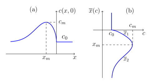
Figure 2: (a) The initial distribution of the local sound velocity $c(x,0)$ in a non-monotonous pulse. (b) Inverse function $\overline{x}(c)$ is two-valued and consist of two branches $\overline{x}_{1}(c)$ and $\overline{x}_{2}(c)$.

Now we can turn to finding the law of motion of the small-amplitude edge of the DSW which propagates with the group velocity equal to, as one can easily obtain,

$$v_{g}=\frac{d\omega}{dk}=2[c(\alpha)-c_{0}]+\alpha^{3}c(\alpha).$$ (28)

According to Whitham whitham-65 ; whitham-74 (see also El05 ; kamch-19 ), this is one of the characteristic velocities of the Whitham modulation equations in the small-amplitude limit. Another characteristic velocity must coincide, evidently, with the dispersionless velocity $v_{+}=3c-2c_{0}$ (see Eq. (19)) and the corresponding Whitham equation separates from the other equations and yields the solution coinciding at the small-amplitude edge with the dispersionless solution (20). The characteristic velocity (28) is the common limiting value of two Whitham velocities at the small-amplitude edge of DSW, so two equations of the Whitham modulation system merge into one equation. Since the value of one more variable is fixed by the Gurevich-Meshcherkin conjecture that the value of one of the dispersionless Riemann invariants is transferred through the DSW, there remains in the small-amplitude limit only two Whitham equations for two parameters $k=k(\alpha)$ and $c$. Consequently, the classical hodograph method is applicable in which $x$ and $t$ are considered as functions of these two parameters $k,c$, and one of these hodograph transformed equations must correspond to the characteristic velocity (28),

$$\frac{\partial x}{\partial c}-[2(c-c_{0})+c\alpha^{3}]\frac{\partial t}{\partial c}=0.$$ (29)

This equation must be compatible with the solution (20) of non-transformed limiting Whitham equations, and this condition gives us the differential equation

$$c(1-\alpha^{3})\frac{dt}{dc}+3t=-\frac{d\overline{x}}{dc}$$ (30)

for the function $t=t(c)$, where $\overline{x}(c)$ is the function inverse to the initial distribution of $c(x)$; see Fig. 1(b). Since we already know the relationship (27) between $c$ and $\alpha$, it is convenient to transform Eq. (30) to the independent variable $\alpha$. To simplify the notation, we introduce the function

$$\Phi(\alpha)=\left.\frac{d\overline{x}}{dc}\right|_{c=c(\alpha)}$$ (31)

and obtain

$$\alpha(1-\alpha^{2})(4-\alpha)\frac{dt}{d\alpha}-3t=\Phi(\alpha).$$ (32)

Its solution is given by

$$\begin{split}t(\alpha)&=\frac{\alpha^{3/4}(4-\alpha)^{1/20}}{(1-\alpha)^{1/2}(1+\alpha)^{3/10}}\\ &\times\int_{1}^{\alpha}\frac{\Phi(z)dz}{z^{7/4}(1-z)^{1/2}(4-z)^{21/20}(1+z)^{7/10}},\end{split}$$ (33)

where it is assumed that the wave breaking takes place at $t=0$ and at the front edge of the pulse where $\alpha=\alpha(c_{0})=1$. When $t=t(\alpha)$ is found, the coordinate of the small-amplitude edge is given by

$$x_{L}(\alpha)=[3c(\alpha)-2c_{0}]t(\alpha)+\overline{x}[c(\alpha)].$$ (34)

The formulas (33) and (34) define in a parametric form the law of motion $x=x_{L}(t)$ of the small-amplitude edge.

Now let us turn to a localized positive pulse when the initial distribution $c(x)$ has a single maximum $c_{m}$ at $x=x_{m}$ and $c(x)\to c_{0}$ fast enough as $x\to-\infty$ and $c(x)\to c_{0}$ with vertical tangent line at $x\to-0$ (see Fig. 2(a)). This means that we suppose again for convenience that the wave breaks at the moment $t=0$. Now there are two branches $\overline{x}_{1,2}(c)$ of the inverse function with $x_{m}<\overline{x}_{1}(c)<0$ and $-\infty<\overline{x}_{2}(c)<x_{m}$ (see Fig. 2(b)). The above formulas obtained for monotonous initial distribution are applicable as long as the small-amplitude edge propagates along the branch $\overline{x}_{1}(c)$, so that the solution can be derived by replacement of the function $\Phi(\alpha)$ by $\Phi_{1}(\alpha)=\left.d\overline{x}_{1}/dc\right|_{c=c(\alpha)}$. When the small-amplitude edge reaches the maximum $c_{m}$ at the moment

$$\begin{split}t_{m}&=\frac{\alpha_{m}^{3/4}(4-\alpha_{m})^{1/20}}{(1-\alpha_{m})^{1/2}(1+\alpha_{m})^{3/10}}\\ &\times\int_{1}^{\alpha_{m}}\frac{\Phi_{1}(z)dz}{z^{7/4}(1-z)^{1/2}(4-z)^{21/20}(1+z)^{7/10}},\end{split}$$ (35)

where $\alpha_{m}$ is the root of the equation $c(\alpha_{m})=c_{m}$, then the equation (32) with $\Phi(\alpha)$ replaced by $\Phi_{2}(\alpha)=\left.d\overline{x}_{2}/dc\right|_{c=c(\alpha)}$ should be solved with the boundary condition

$$t(\alpha_{m})=t_{m}.$$ (36)

Hence, for $t>t_{m}$ the motion of the small-amplitude is determined by the formulas

$$\begin{split}&t(\alpha)=\frac{\alpha^{3/4}(4-\alpha)^{1/20}}{(1-\alpha)^{1/2}(1+\alpha)^{3/10}}\\ &\times\Bigg{\{}\int_{1}^{\alpha_{m}}\frac{\Phi_{1}(z)dz}{z^{7/4}(1-z)^{1/2}(4-z)^{21/20}(1+z)^{7/10}}\\ &+\int_{\alpha_{m}}^{\alpha}\frac{\Phi_{2}(z)dz}{z^{7/4}(1-z)^{1/2}(4-z)^{21/20}(1+z)^{7/10}}\Bigg{\}},\\ &x_{L}(\alpha)=[3c(\alpha)-2c_{0}]t(\alpha)+\overline{x}_{2}(c).\end{split}$$ (37)

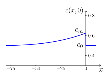
Figure 3: The initial distribution of the local sound velocity $c(x,0)$ given by Eq. (50) with parameters $c_{0}=0.5$, $c_{1}=0.005$, $x_{0}=100$.

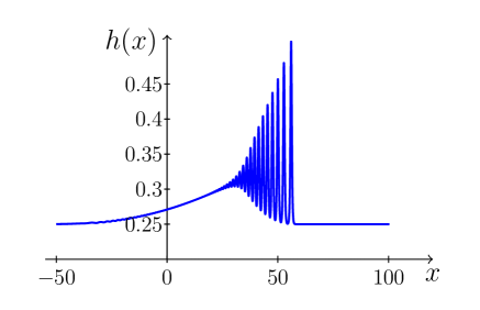
Figure 4: A typical surface elevation $h(x)$ at fixed moment of time $t=80$ in the pulse evolved from the initial distribution (50) found by numerical solution of the Serre equations.

The law of motion of the soliton edge of DSW cannot be found by this method, since the relation (3) does not hold during evolution of the pulse. However, as was remarked in Ref. kamch-19 , this relationship can be used in vicinity of the moment when the small-amplitude edge reaches the point with $c=c_{m}$. We rewrite Eq. (12) in the form

$$\widetilde{\omega}(\widetilde{k})=u\widetilde{k}+\widetilde{k}c(1-c^{4}\widetilde{k}^{2}/3)^{-1/2}=\widetilde{k}[u+c\widetilde{\alpha}(\widetilde{k})],$$ (38)

that is

$$\widetilde{\alpha}(\widetilde{k})=(1-c^{4}\widetilde{k}^{2}/3)^{-1/2},\qquad(\widetilde{\alpha}>1),$$

and then

$$\widetilde{k}(c)=\frac{\sqrt{3}}{c^{2}}\sqrt{1-\frac{1}{\widetilde{\alpha}^{2}}}.$$ (39)

Substitution of these expressions into Eq. (3) with account of $u=u(c)$ yields the familiar differential equation

$$\frac{d\widetilde{\alpha}}{dc}=-\frac{\widetilde{\alpha}(4-\widetilde{\alpha})(1+\widetilde{\alpha})}{c(1+\widetilde{\alpha}+\widetilde{\alpha}^{2})}$$ (40)

coinciding with Eq. (25). Now we extrapolate it to the whole DSW what allows us to solve it with the boundary condition

$$\widetilde{\alpha}(c_{m})=1,$$ (41)

which means that the solitons widths become infinitely large ($\widetilde{k}\to 0$) and their amplitude infinitely small at the small-amplitude edge. Then the solution of the differential equation coincides with Eq. (27) after obvious replacements $\alpha\to\widetilde{\alpha}$, $c_{0}\to c_{m}$,

$$c(\widetilde{\alpha})=\frac{c_{m}}{2^{1/5}3^{21/20}}\cdot\frac{(1+\widetilde{\alpha})^{1/5}(4-\widetilde{\alpha})^{21/20}}{\widetilde{\alpha}^{1/4}}.$$ (42)

Here $c<c_{m}$, $\widetilde{\alpha}$ increases with decrease of $c$ and reaches its maximal value at $c=c_{0}$ which corresponds to the maximal possible value of the soliton velocity equal to

$$v_{R}=\left.\frac{\widetilde{\omega}}{\widetilde{k}}\right|_{c=c_{0}}=c_{0}\widetilde{\alpha}(c_{0}).$$ (43)

This value of the leading soliton velocity in DSW is reached at large enough time when solitons near the leading edge are well separated from each other and propagate along the constant background with $c=c_{0}$. Substitution of $\widetilde{\alpha}(c_{0})=v_{R}/c_{0}$ into Eq. (42) yields the equation

$$\frac{v_{R}}{c_{0}}=\left(\frac{c_{m}}{c_{0}}\right)^{4}\left(\frac{1+v_{R}/c_{0}}{2}\right)^{4/5}\left(\frac{4-v_{R}/c_{0}}{3}\right)^{21/5},$$ (44)

which determines implicitly the value of $v_{R}$ in terms of $c_{0}$ and $c_{m}$. This equation coincides actually with the equation obtained in Ref. egs-06 for velocity of the leading soliton in a bore generated from a step-like initial distribution what should be expected since such a distribution can be modeled by a long enough pulse with a sharp front. When the velocity of the leading soliton is found, its amplitude is given by (see Eq. (13))

$$a=v_{R}^{2}-h_{0}=h_{0}\left[\widetilde{\alpha}^{2}\left(\sqrt{h_{0}}\right)-1\right]$$ (45)

in agreement with the result obtained in Ref. egs-08 for asymptotic stage of evolution of positive pulses.

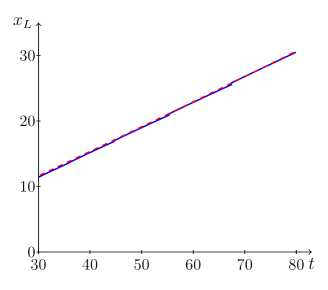
Figure 5: A path of the small-amplitude edge in DSW generated by the initial distribution (50) shown in Fig. 3. The numerical results are depicted by a solid (blue) line. The analytical curve corresponds to Eqs. (37) and it is shown by dashed (red) line.

It is instructive to compare the formulas of the Serre equations theory with the results obtained in the small nonlinearity approximation when propagation of the pulse obeys the KdV equation

$$\begin{split}&u_{t}+\sqrt{gh_{0}}\left(u_{x}+\frac{1}{6}h_{0}^{2}u_{xxx}\right)+\frac{3}{2}uu_{x}=0,\\ &u=2(c-c_{0}).\end{split}$$ (46)

A similar calculation yields (see Ref. kamch-19 )

$$\begin{split}&t(c)=-\frac{1}{6\sqrt{c-c_{0}}}\Big{\{}\int_{c_{0}}^{c_{m}}\frac{\overline{x}_{1}^{\prime}(c)dc}{\sqrt{c-c_{0}}}+\int_{c_{m}}^{c}\frac{\overline{x}_{2}^{\prime}(c)dc}{\sqrt{c-c_{0}}}\Big{\}},\\ &x_{L}(\alpha)=[3c(\alpha)-2c_{0}]t(\alpha)+\overline{x}_{2}(c).\end{split}$$ (47)

Naturally, these formulas correspond to the approximation of the function $c(\alpha)$

$$\begin{split}&c(\alpha)\approx c_{0}[1+(1-\alpha)/2],\quad\text{that is}\\ &\alpha(c)\approx 3-2c/{c_{0}},\end{split}$$ (48)

and can be obtained from Eqs. (37) by substitution into them of this leading approximation of the function $\alpha(c)$.

In a similar way, in the KdV approximation Eq. (44) yields the asymptotic value of the leading soliton velocity

$$v_{R}\approx 2c_{m}-c_{0}.$$ (49)

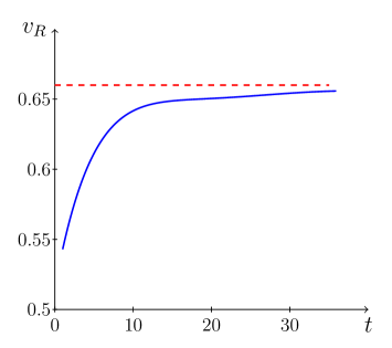
Figure 6: Velocity of the soliton edge as a function of time (solid blue line). Dashed (red) line indicates the asymptotic value of the velocity of this edge given by Eq. (43).

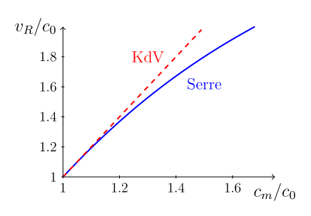
Figure 7: Comparison of velocity $v_{R}/c_{0}$ of the leading soliton according to the Serre theory (Eq. (43); solid blue line) and the KdV equation theory (Eq. (49); dashed red line) as functions of the amplitude $c_{m}/c_{0}$ of the initial pulse.

We have compared our analytical approach to DSWs in the Serre equations theory with their numerical solution for the pulse with $x_{m}=0$, sharp front edge and long enough rear distribution described by the function (see Fig. 3)

$$c(x)=c_{0}+[c_{1}(x+x_{0})]^{3},$$ (50)

so that

$$\begin{split}&\overline{x}_{2}(c-c_{0})=(c-c_{0})^{1/3}/{c_{1}}-x_{0},\\ &\Phi_{2}(\alpha)=[c(\alpha)-c_{0}]^{-2/3}/(3c_{1}).\end{split}$$ (51)

The typical wave pattern for the water elevation evolved from such a pulse is shown in Fig. 4. It is worth noticing that the amplitude of the wave has the same order of magnitude as the background depth, that is the KdV approximation is not applicable in this case. Propagation path of the small-amplitude edge is depicted in Fig. 5. Since the Whitham asymptotic theory does not take into account the initial stage of formation of the DSW, the analytical curve is shifted slightly upwards to match the numerical one. As we see, this single fitting parameter permits one to describe the whole curve very well.

Dependence of the leading soliton velocity on time is shown in Fig. 6. As we see, it approaches with time to its asymptotic value given by Eq. (43). At last, in Fig. 7 we compare the dependence of velocity of the leading soliton on the amplitude $c_{m}/c_{0}$ of the initial pulse according to the Serre theory (solid line) and Korteweg-de Vries theory (dashed line). As one can see, the difference between two approximations increases very fast with growth of the amplitude.

Thus, our analytical approach agrees quite well with velocities of propagation of the edges of DSW evolved from arbitrary enough initial profile of the pulse in the Serre equation theory.

IV Negative pulse

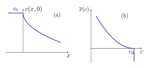
Figure 8: (a) The initial distribution of the local sound velocity $c(x,0)$ in a monotonous negative pulse. (b) Inverse function $\overline{x}(c)$.

Here we turn to the discussion of evolution of a “negative” pulse with a dip in the initial distribution of the local sound velocity $c(x)$. Again we shall start from a monotonous pulse with the initial distribution of the local sound velocity

$$c(x,0)=\begin{cases}c_{0}&\mbox{if}\quad x<0,\\ c_{0}-\widetilde{c}(x)&\mbox{if}\quad x\geq 0,\end{cases}$$ (52)

which is shown in Fig. 8(a), and the inverse function $\overline{x}(c)$ shown in Fig. 8(b). As was indicated in Ref. kamch-19 , in situations of this kind Eq. (3) is fulfilled at the soliton edge located at the boundary with the smooth part of the pulse which is described in dispersionless approximation by Eq. (20). This smooth part acquires with time a triangle-like shape which is well known in the KdV equation theory (see, e.g. as-77 ; dvz-94 ; ikp-18 ) and in the “shallow water” system derived as a dispersionless approximation in the NLS equation theory (see, e.g., ikp-19 ). As in Refs. El05 ; kamch-19 , we assume that Eq. (3) is valid also for DSWs propagating into a quiescent medium and apply this conjecture to description of DSW evolved from the initial distribution (52) according to the Serre equations. Then Eq. (3) can be transformed in the same way as it was done in Eqs. (38)-(40), but now Eq. (40) must be solved with the boundary condition

$$\widetilde{\alpha}(c_{0})=1$$ (53)

since in the case of negative initial pulse the small-amplitude edge of the DSW is located at the boundary with the quiescent medium where $c=c_{0}$ and solitons amplitude tends to zero as $c\to c_{0}$. The solution is obtained from Eq. (42) by a replacement $c_{m}\to c_{0}$, i.e.,

$$c(\widetilde{\alpha})=\frac{c_{0}}{2^{1/5}3^{21/20}}\cdot\frac{(1+\widetilde{\alpha})^{1/5}(4-\widetilde{\alpha})^{21/20}}{\widetilde{\alpha}^{1/4}},$$ (54)

where $\widetilde{\alpha}>1$. When the function $\widetilde{\alpha}(c)$ is known, the velocity of the front edge can be represented as the soliton velocity

$$v_{R}=\frac{\widetilde{\omega}}{\widetilde{k}}=2(c-c_{0})+c\widetilde{\alpha}.$$ (55)

We notice again that $v_{R}$ is the characteristic velocity of the Whitham modulation equations at the soliton edge. The corresponding Whitham equation can be written in the hodograph transformed form

$$\frac{\partial x}{\partial c}-[2(c-c_{0})+c\widetilde{\alpha}]\frac{\partial t}{\partial c}=0.$$ (56)

The condition that this equation must be compatible with the solution (20) of the dispersionless approximation at the soliton edge of the DSW yields the differential equation for the function $t=t(c)$ at this edge,

$$c(\widetilde{\alpha}-1)\frac{dt}{dc}-3t=\frac{d\overline{x}}{dc}.$$ (57)

Introducing the function $\Phi(\widetilde{\alpha})=\left.d\overline{x}/dc\right|_{c=c(\widetilde{\alpha}}$ we cast it to the form

$$\frac{\widetilde{\alpha}(\widetilde{\alpha}^{2}-1)(4-\widetilde{\alpha})}{1+\widetilde{\alpha}+\widetilde{\alpha}^{2}}\frac{dt}{d\widetilde{\alpha}}+3t=-\Phi(\widetilde{\alpha})$$ (58)

with $\widetilde{\alpha}$ as an independent variable. Since we assume that the initial profile breaks at the moment $t=0$ at the rear edge where $c=c_{0}$, i.e., $\widetilde{\alpha}=1$, this equation should be solved with the boundary condition

$$t(1)=0.$$ (59)

As a result, we obtain

$$\begin{split}t(\widetilde{\alpha})=&-\frac{\widetilde{\alpha}^{3/4}(4-\widetilde{\alpha})^{21/20}}{(\widetilde{\alpha}-1)^{3/2}(\widetilde{\alpha}+1)^{3/10}}\\ &\times\int_{1}^{\widetilde{\alpha}}\frac{\Phi(z)(1+z+z^{2})(z-1)^{1/2}dz}{z^{7/4}(z+1)^{7/10}(4-z)^{41/20}}.\end{split}$$ (60)

The coordinate of the soliton edge is given by

$$x_{R}(\widetilde{\alpha})=[3c(\widetilde{\alpha})-2c_{0}]t(\widetilde{\alpha})+\overline{x}[c(\widetilde{\alpha})],$$ (61)

so that Eqs. (60), (61) define the law of motion $x=x_{R}(t)$ of this edge in parametric form.

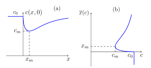
Figure 9: (a) The initial distribution of the local sound velocity $c(x,0)$ in a nonmonotonous negative pulse. (b) Inverse function $\overline{x}(c)$.

Generalization of this theory on localized pulses (see Fig. 9(a)) is straightforward. Now we have a two-valued inverse function which consists of two branches $\overline{x}_{1}(c)$ and $\overline{x}_{2}(c)$ (see Fig. 9(b)). Equations (60), (61) with $\Phi$ replaced by $\Phi_{1}(\widetilde{\alpha})=\left.d\overline{x}_{1}/dc\right|_{c=c(\widetilde{\alpha}}$ are valid up to the moment

$$\begin{split}t_{m}=&-\frac{\widetilde{\alpha}^{3/4}(4-\widetilde{\alpha})^{21/20}}{(\widetilde{\alpha}-1)^{3/2}(\widetilde{\alpha}+1)^{3/10}}\\ &\times\int_{1}^{\widetilde{\alpha}_{m}}\frac{\Phi_{1}(z)(1+z+z^{2})(z-1)^{1/2}dz}{z^{7/4}(z+1)^{7/10}(4-z)^{41/20}}\end{split}$$ (62)

when the soliton edge reaches the minimum $c_{m}$ in the distribution of the local sound velocity and $\widetilde{\alpha}_{m}$ is defined by the equation $c(\widetilde{\alpha}_{m})=c_{m}$. After that moment $t>t_{m}$ the soliton edge propagates along the second branch $\overline{x}_{2}(c)$ and the law of motion of this edge is defined by the equations

$$\begin{split}t(\widetilde{\alpha})=&-\frac{\widetilde{\alpha}^{3/4}(4-\widetilde{\alpha})^{21/20}}{(\widetilde{\alpha}-1)^{3/2}(\widetilde{\alpha}+1)^{3/10}}\\ &\times\Bigg{\{}\int_{1}^{\widetilde{\alpha}_{m}}\frac{\Phi_{1}(z)(1+z+z^{2})(z-1)^{1/2}dz}{z^{7/4}(z+1)^{7/10}(4-z)^{41/20}}\\ &+\int_{\widetilde{\alpha}_{m}}^{\widetilde{\alpha}}\frac{\Phi_{2}(z)(1+z+z^{2})(z-1)^{1/2}dz}{z^{7/4}(z+1)^{7/10}(4-z)^{41/20}}\Bigg{\}},\\ x_{R}(\widetilde{\alpha})&=[3c(\widetilde{\alpha})-2c_{0}]t(\widetilde{\alpha})+\overline{x}_{2}[c(\widetilde{\alpha})].\end{split}$$ (63)

At asymptotically large time $t\to\infty$ we have $\widetilde{\alpha}\to 1$ and $t(\widetilde{\alpha})\approx\mathcal{A}/(\widetilde{\alpha}-1)^{3/2}$, where

$$\mathcal{A}=-\frac{3^{21/20}}{2^{3/10}}\int\frac{\Phi(z)(1+z+z^{2})(z-1)^{1/2}dz}{z^{7/4}(z+1)^{7/10}(4-z)^{41/20}},$$ (64)

where the integral should be taken over the whole initial pulse ($\int\Phi=\int_{1}^{\widetilde{\alpha}_{m}}\Phi_{1}+\int_{\widetilde{\alpha}_{m}}^{1}\Phi_{2}$). In this limit $c(\widetilde{\alpha})\approx c_{0}[1-(\widetilde{\alpha}-1)/2]$ and simple calculation yields

$$x_{R}(t)\approx c_{0}t-\frac{3}{2}\mathcal{A}^{2/3}t^{1/3}.$$ (65)

This asymptotic law of motion coincides actually with the corresponding law in the KdV equation theory but with a different value of the constant $\mathcal{A}$ (see Ref. ikp-18 ).

The method of Ref. kamch-19 permits us to find asymptotic value of velocity of the rear small-amplitude edge at $t\to\infty$. To this end, we have to solve Eq. (25) with the boundary condition

$$\alpha(c_{m})=1$$ (66)

which means that at the moment when the soliton edge reaches the minimum of distribution of $c(x)$, the wave number here given by Eq. (23) tends to zero. This gives

$$c(\alpha)=\frac{c_{m}}{\alpha^{1/4}}\left(\frac{1+\alpha}{2}\right)^{1/5}\left(\frac{4-\alpha}{3}\right)^{21/20}.$$ (67)

At the small amplitude edge we have $c=c_{0}$ and the group velocity (28) plays the role of the left-edge velocity,

$$v_{L}=\alpha_{0}^{3}c_{0},$$ (68)

where $c_{0}=c(\alpha_{0})$. Substitution of $\alpha_{0}=(v_{L}/c_{0})^{1/3}$ into Eq, (67) yields the equation

$$\left(\frac{v_{L}}{c_{0}}\right)^{\frac{1}{12}}=\frac{c_{m}}{c_{0}}\left[\frac{1+(v_{L}/c_{0})^{\frac{1}{3}}}{2}\right]^{\frac{1}{5}}\left[\frac{3-(v_{L}/c_{0})^{1/3}}{3}\right]^{\frac{21}{20}}$$ (69)

which determines $v_{L}$ in terms of $c_{0}$ and $c_{m}$. In the KdV approximation Eq. (69) gives

$$v_{L}\approx 6c_{m}-5c_{0}.$$ (70)

This relation agrees with the corresponding result of Ref. ikp-18 after its transformation to physical variables of Eq. (46).

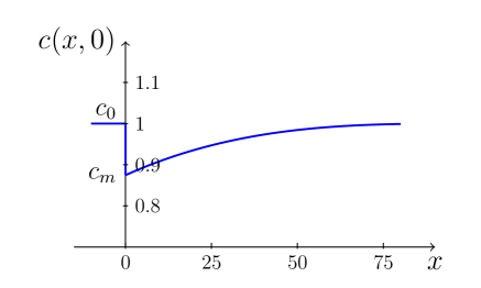
Figure 10: The initial distribution of the local sound velocity $c(x,0)$ given by Eq. (71) with parameters $c_{0}=0.5$, $c_{1}=0.005$, $x_{0}=100$.

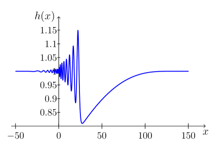
Figure 11: A typical surface elevation $h(x)$ at fixed moment of time $t=30$ in the pulse evolved from the initial distribution (71) found by numerical solution of the Serre equations.

We compared our analytical approach to DSWs in the Serre equations theory with their numerical solution for the pulse with the initial distribution of the local sound velocity defined by the equation (see Fig. 10)

$$c(x)=c_{0}-[c_{1}(-x+x_{0})]^{3},$$ (71)

so that

$$\begin{split}&\overline{x}_{2}(c)=x_{0}-(c_{0}-c)^{1/3}/{c_{1}},\\ &\Phi_{2}(\alpha)=[c_{0}-c(\alpha)]^{-2/3}/(3c_{1}).\end{split}$$ (72)

The typical wave pattern for the water elevation evolved from such a pulse is shown in Fig. 11. As was mentioned above, the smooth part of the pulse acquires a triangle-like shape in agreement with typical behavior of dispersionless solutions of shallow water equations (14).

Propagation path of the soliton edge is depicted in Fig. 12. Again the analytical curve is shifted slightly upwards to match the numerical one. As we see, this single fitting parameter permits one to describe the whole curve very well.

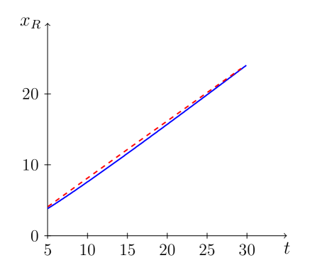
Figure 12: Propagation path of the soliton edge: numerical results are shown by a solid (blue) line and analytical calculation by a dashed (ref) line.

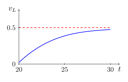
Figure 13: Dependence of the velocity of the small-amplitude edge on time: numerical results are shown by a solid (blue) line and the analytical asymptotic value (68) by a dashed (red) line.

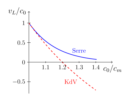
Figure 14: Dependence of the velocity of the small-amplitude edge according to the Serre theory (upper blue line) and to the KdV approximation (lower red line).

Dependence of the velocity of the small-amplitude edge on time is shown in Fig. 13. As we see, it approaches with time to the asymptotic law of motion with the constant velocity given by Eq. (68). At last, in Fig. 14 we compare the dependence of velocity of the small-amplitude edge on the parameter $c_{0}/c_{m}$ according to the Serre theory (upper blue line) and Korteweg-de Vries theory (lower red line). As one can see, again the difference between two approximations increases very fast with growth of depth of the dip in the initial distribution.

V Conclusion

We have studied evolution of dispersive shock waves formed after wave breaking of simple-wave pulses in the fully nonlinear shallow-water approximation in framework of the Serre equations model with the use of the Whitham modulation theory. Formation of undular bores from initial step-like distributions was studied earlier in Ref. egs-06 and asymptotic stage of positive initial pulses at the large enough time, when it evolves to a train of well separated solitons, was studied in Ref. egs-08 . The present study essentially extends such an approach to much wider class of initial conditions with both types of possible polarities (humps and dips in initial elevations) and to any value of time evolution provided the Whitham method is applicable. In particular, we have obtained the laws of motion of the small-amplitude edge of DSW evolved from a positive pulse and the law of motion of the soliton edge of DSW evolved from negative pulse, when velocities of these edges depend on the initial profiles of the pulses and they are given by simple analytical formulas. Especially useful in practical applications may be formulas for velocities of the edges at asymptotically large time. In addition to the leading soliton velocity generated by a positive pulse which was already found in Ref. egs-08 , we have found the small-amplitude velocity for the same initial polarity and expressions for both edges in the case of negative polarity. Remarkably enough, these asymptotical velocities depend on a single parameter given by either a certain integral over the initial distribution, or its extremal value within the initial pulse. We hope that the developed here theory can find applications to description of experimental investigations of water waves of the type performed in Refs. hs-78 ; clauss-99 ; tkco-16 . The developed theory demonstrates quite clearly that the method suggested in Ref. kamch-19 is convenient enough for discussion of concrete situations and it can be effectively applied to various models of water wave physics and other nonlinear physics problems.

- (1) L. N. Debnath, Nonlinear Water Waves, Academic Press, London, 1994.
- (2) R. S. Johnson, A Modern Introduction to the Mathematicsl Theory of Water Waves, Cambridge, UP, 1997.
- (3) J. R. Apel, L. A. Ostrovsky, Y. A. Stepanyants, J. F. Linch, J. Acoust. Soc. Am., 121, 695 (2007).
- (4) Q. Ma (Ed.) Advances in Numerical Simulation of Nonlinear Water Waves, World Scientific, Singapore, 2010.
- (5) N. Paldor, Shallow Water Waves on the Rotating Earth, Springer, N. Y., 2015.
- (6) N. Abcha, E. Pelinovsky, and I. Mutabazi (Eds.), Nonlinear Waves and Pattern Dynemics, Springer, N. Y., 2018.
- (7) D. J. Korteweg and G. de Vries, Phil. Mag., 39, 422 (1895).
- (8) T. B. Benjamin and M. J. Lighthill, Proc. Roy. Soc. London, A 224, 448 (1954).
- (9) G. B. Whitham, Proc. Roy. Soc. London, A 283, 238 (1965), \doi10.1098/rspa.1965.0019.
- (10) G. B. Whitham, Linear and Nonlinear Waves (Wiley Interscience, New York, 1974).
- (11) A. V. Gurevich and L. P. Pitaevskii, Zh. Eksp. Teor. Fiz. 65, 590 (1973) [Sov. Phys. JETP 38, 291 (1974)].
- (12) A. V. Gurevich, A. L. Krylov and G. A. El, Pis’ma Zh. Eksp. Teor. Fiz. 54, 104 (1991) [JETP Lett. 54, 102 (1991)].
- (13) A. V. Gurevich, A. L. Krylov and G. A. El, Zh. Eksp. Teor. Fiz. 101, 1797 (1992) [Sov. Phys. JETP 74, 957 (1992)].
- (14) A. L. Krylov, V. V. Khodorovskii and G. A. El, Pis’ma Zh. Eksp. Teor. Fiz. 56, 325 (1992) [JETP Lett. 56, 323 (1992)].
- (15) O. C. Wright, Commun. Pure Appl. Math. 46, 423 (1993) \doi10.1002/cpa.3160460306
- (16) F. R. Tian, Commun. Pure Appl. Math. 46, 1093 (1993) \doi10.1002/cpa.3160460802.
- (17) V. I. Karpman, Phys. Lett. A 25, 708 (1967), \doi10.1016/0375-9601(67)90953-X.
- (18) M. J. Ablowitz and A. C. Newell, J. Math. Phys. 14, 1277 (1973), \doi10.1063/1.1666479.
- (19) V. E. Zakharov and S. V. Manakov, Zh. Eksp. Teor. Fiz. 71, 203 (1976) [Sov. Phys. JETP, 44, 106 (1976)].
- (20) M. J. Ablowitz and H. Segur, Stud. Appl. Math. 57, 13 (1977), \doi10.1002/sapm197757113.
- (21) H. Segur and M. J. Ablowitz, Physica D 3, 165 (1981) \doi10.1016/0167-2789(81)90124-X
- (22) G. A. El and V. V. Khodorovsky, Phys. Lett. A 182, 49 (1993), \doi10.1016/0375-9601(93)90051-Z.
- (23) P. Deift, S. Venakides, and Z. Zhou, Commun. Pure Appl. Math. 47, 199 (1994), \doi10.1002/cpa.3160470204.
- (24) G. A. El, A. L. Krylov, and S. Venakides, Commun. Pure Appl. Math. 54, 1243 (2001), \doi10.1002/cpa.10002.
- (25) T. Claeys and T. Grava, Commun. Math. Phys. 286, 979 (2009), \doi10.1007/s00220-008-0680-5.
- (26) T. Claeys and T. Grava, Commun. Pure Appl. Math. 63, 203 (2010), \doi10.1002/cpa.20277.
- (27) M. Isoard, A. M. Kamchatnov, and N. Pavloff, Phys. Rev. E 99, 012210 (2019), \doi10.1103/PhysRevE.99.012210.
- (28) J. L. Hammack and H. Segur, J. Fluid Mech. 65, 289 (1974) \doi10.1017/S002211207400139X; ibid., J. Fluid Mech. 84, 337 (1978) \doi10.1017/S0022112078000208.
- (29) G. F. Clauss, Appl. Ocean Res. 21, 219 (1999).
- (30) J. S. Antunes do Carmo, J. Hydraulic Res., 51, 719 (2013).
- (31) S. Trillo, M. Klein, G. F. Clauss, M. Onorato, Physica D 333, 276 (2016) \doi10.1016/j.physd.2016.01.007.
- (32) F. Serre, La Houille Blanche, 8, 374-388, 830-887 (1953).
- (33) C. H. Su and C. S. Gardner, J. Math. Phys., 10, 536 (1969).
- (34) A. E. Green and P. M. Naghdi, J. Fluid Mech., 78, 237 (1976).
- (35) A. V. Gurevich and A. P. Meshcherkin, Zh. Eksp. Teor. Fiz., 87, 1277-1292 (1984) [Sov. Phys. JETP, 60, 732-740 (1984)].
- (36) G. A. El, Chaos 15, 037103 (2005), \doi10.1063/1.1947120; ibid. 16, 029901 (2006), \doi10.1063/1.2186766.
- (37) O. Akimoto and K. Ikeda, J. Phys. A: Math. Gen., 10, 425 (1977); K. Ikeda and O. Akimoto, J. Phys. A: Math. Gen. 12, 1105 (1979).
- (38) S. A. Darmanyan, A. M. Kamchatnov, M. Neviére, Zh. Eksp. Teor. Fiz., 123, 997-1005 (2003) [JETP, 96, 876–884 (2003)].
- (39) G. A. El, A. Gammal, E. G. Khamis, R. A. Kraenkel, A. M. Kamchatnov, Phys. Rev. A 76, 053813 (2007), \doi10.1103/PhysRevA.76.053813.
- (40) J. G. Esler, J. D. Pearce, J. Fluid Mech., 667, 555-585 (2011), \doi10.1017/S0022112010004593.
- (41) M. A. Hoefer, J. Nonlinear Sci., 24, 525-577 (2014) \doi10.1007/s00332-014-9199-4.
- (42) M. A. Hoefer, G. A. El, A. M. Kamchatnov, SIAM J. Appl. Math., 77, 1352-1374 (2017) \doi10.1137/16M108882X.
- (43) G. A. El, R. H. J. Grimshaw, N. F. Smyth, Phys. Fluids, 18, 027104 (2006), \doi10.1063/1.2175152.
- (44) G. A. El, R. H. J. Grimshaw, N. F. Smyth, Physica D, 237, 2423-2435 (2008), \doi10.1016/j.physd.2008.03.031.
- (45) A. M. Kamchatnov, R. A. Kraenkel, B. A. Umarov, Phys. Rev. E 66, 036609 (2002).
- (46) A. M. Kamchatnov, R. A. Kraenkel, B. A. Umarov, Wave Motion 38, 355-365 (2003).
- (47) A. V. Gurevich, A. L. Krylov, and N. G. Mazur, Zh. Eksp. Teor. Fiz. 95, 1674 (1989) [Sov. Phys. JETP 68, 966 (1989)].
- (48) A. M. Kamchatnov, Zh. Eksp. Teor. Fiz. 154, 1016, (2018), \doi10.1134/S0044451018110111 [JETP, 127, 903-911 (2018), \doi10.1134/S1063776118110043].
- (49) A. M. Kamchatnov, Nonlinear Periodic Waves and Their Modulations—An Introductory Course, (World Scientific, Singapore, 2000).
- (50) A. M. Kamchatnov, Phys. Rev. E 99, 012203 (2019), \doi10.1103/PhysRevE.99.012203.
- (51) M. Isoard, A. M. Kamchatnov, and N. Pavloff, arxiv:1902.06975 (2019).