Structure and Expansion Law of H II Regions in structured Molecular Clouds

Abstract

We present radiation-magnetohydrodynamic simulations aimed at studying evolutionary properties of H II regions in turbulent, magnetised, and collapsing molecular clouds formed by converging flows in the warm neutral medium. We focus on the structure, dynamics and expansion laws of these regions. Once a massive star forms in our highly structured clouds, its ionising radiation eventually stops the accretion (through filaments) toward the massive star-forming regions. The new over-pressured H II regions push away the dense gas, thus disrupting the more massive collapse centres. Also, because of the complex density structure in the cloud, the H II regions expand in a hybrid manner: they virtually do not expand toward the densest regions (cores), while they expand according to the classical analytical result towards the rest of the cloud, and in an accelerated way, as a blister region, towards the diffuse medium. Thus, the ionised regions grow anisotropically, and the ionising stars generally appear off-centre of the regions. Finally, we find that the hypotheses assumed in standard H II-region expansion models (fully embedded region, blister-type, or expansion in a density gradient) apply simultaneously in different parts of our simulated H II regions, producing a net expansion law ($R\propto t^{\alpha}$, with $\alpha$ in the range of 0.93-1.47 and a mean value of $1.2\pm 0.17$) that differs from any of those of the standard models.

1 Introduction

Massive stars play a key role in the evolution of galaxies. Through a combination of massive outflows, expanding Hii regions, and supernova explosions, they shape and provide an important input of energy to the interstellar medium (ISM; e.g., Mac Low & Klessen, 2004). In particular, they erode and disperse their parent molecular clouds (MCs), directly affecting the star formation activity within the clouds (see, e.g., Krumholz et al., 2014; Vázquez-Semadeni, 2015, for recent reviews).

It is generally thought that the negative feedback through blister-type Hii regions (or “champagne” flows; Franco et al., 1990) is efficient in eroding and dispersing MCs on timescales of few tens of Myr (Blitz & Shu, 1980; Matzner, 2002). Idealised analytical (e.g., Whitworth, 1979; Franco et al., 1994, hereafter, we will refer to the latter work as FST94) and numerical (e.g. Bodenheimer et al., 1979; Tenorio-Tagle, 1979) works have shown that blister Hii regions are also able to reduce the star formation efficiency (SFE) of MCs to the low observed values of $\lesssim 10$% (e.g., Myers et al., 1986). However, all these simplified models without self-gravity, with plane-parallel geometry and/or uniform density fields are far from the complex morphology and dynamics observed in MCs (see, e.g., André et al., 2013, for a recent review), which includes turbulence, magnetic fields and anisotropic and hierarchical collapse, leading to the formation of filamentary structures that funnel gas to the star-forming sites (e.g., Gómez & Vázquez-Semadeni, 2014; Smith et al., 2016; Vázquez-Semadeni et al., 2017, although see Matzner & Jumper 2015 for an exception).

Furthermore, the dynamics (free-fall motions or accretion) and the high-density environment of the birthplaces of massive stars could strongly attenuate the disruptive effect of the massive stars (Yorke et al., 1989; Dale et al., 2005; Peters et al., 2010). This picture gets more complicated if we take into account that MCs could be in global collapse, as recent and growing evidence shows (see, e.g., Hartmann et al., 2001; Burkert & Hartmann, 2004; Hartmann & Burkert, 2007; Peretto et al., 2007; Vázquez-Semadeni et al., 2007; Vázquez-Semadeni et al., 2009; Galván-Madrid et al., 2009; Schneider et al., 2010; Csengeri et al., 2011; Ballesteros-Paredes et al., 2011; Hartmann et al., 2012; Ballesteros-Paredes et al., 2015; Peretto et al., 2014; Juárez et al., 2017).

In a medium with power law density stratification $r^{-p}$, with $p>3/2$, Franco et al. (1990) showed analytically that Hii regions expand in an accelerated way. Arthur & Hoare (2006), using numerical simulations of Hii regions expanding in a stratified medium that decreases exponentially, showed that a very weak shock develops toward the densest part of the cloud. This result is crucial in interpreting analytical models in the literature (see App. A).

At scales of MCs, recent numerical simulations (regardless of the initial conditions or setup) of highly-structured clouds have shown that negative feedback is able to reduce the SFE of MCs to values consistent with the observations (e.g., Dale et al., 2005; Walch et al., 2012; Colín et al., 2013; Geen et al., 2015). The effect of the ionising feedback depends strongly on the clouds’ masses and sizes, being weaker for more massive clouds (Dale et al., 2012). However, simulations investigating this effect on clouds of various masses generally tend to assume idealised, spherical initial mass distributions, which are not necessarily realistic, since it is known that clouds tend to be sheet-like and filamentary (e.g., Bally et al., 1987; André et al., 2013). Thus, it is important to investigate the effect of stellar feedback in realistically-shaped clouds, whose morphology is dictated self-consistently by their evolution since their formation.

In contrast, several observational studies have attempted to infer empirical correlations between physical properties of Hii regions, such as density and size. For example, Hunt & Hirashita (2009) studied extragalactic Hii regions and compiled data from both Galactic (Garay & Lizano, 1999; Kim & Koo, 2001; Martín-Hernández et al., 2003; Dopita et al., 2006) and extragalactic (Kennicutt, 1984; Gilbert & Graham, 2007) samples, concluding that the entire sample follows a size ($R_{\rm i}$) versus ionised gas density ($n_{i}$) trend of the form $n_{i}\propto R_{\rm i}^{-1}$, although with a considerable dispersion. Interestingly, combining this relation and the Larson correlation ($n_{\rm H_{2}}\propto R_{\rm H_{2}}^{-1.1}$; where $n_{\rm H_{2}}$ and $R_{\rm H_{2}}$ are the density and size of a given MC) these authors suggest that the star formation is a scale-free process. However, there have been claims in the literature that the Larson density-size correlation is only the result of a selection effect due to the criteria used for defining a MC and their rapidly decaying column density PDFs (Ballesteros-Paredes et al. (2012), see also Kegel (1989); Scalo (1990); Vázquez-Semadeni et al. (1997); Ballesteros-Paredes & Mac Low (2002); Heyer et al. (2009); Camacho et al. (2016) for other possibilities).

In order to study the evolutionary properties of individual Hii regions embedded in realistically structured MCs, we present in this contribution radiation-magnetohydrodynamic (RMHD) simulations of MCs formed by converging flows, that evolve self-consistently, from their formation to their destruction by ionising radiation. Because of this self-consistent evolution, the clouds also have a realistic spatial structure, which, rather than spherical, is closer to being sheet-like, and highly inhomogeneous. In this work, we also study the time evolution of the size-density relation of the ionised gas.

We organise the paper as follows. In §2, we describe the numerical model. In §3 and 4 we present our results, which are then discussed in §5. Finally, the summary and conclusions are presented in §6.

2 The numerical model

With the goal of investigating the effect of magnetic fields in the formation and evolution of MCs, in Zamora-Avilés et al. (2018, hereafter Paper I) we presented three-dimensional, self gravitating, MHD simulations of MCs formed by two WNM colliding flows, including heating and cooling processes. These simulations were carried out using the Eulerian adaptive mesh refinement FLASH (v2.5) code (Fryxell et al., 2000).

In this contribution we consider one of those models (labelled B3), in which the magnitude of the magnetic field (initially uniform) is $3\mu$G in our WNM-like initial conditions. This value is consistent with the observed mean value magnetic field of the uniform component in the Galaxy (Beck, 2001). In addition, we present an additional simulation including radiative transfer, in order to model the effects of UV feedback from massive stars. For this, we use the radiation scheme introduced by Rijkhorst et al. (2006) and improved by Peters et al. (2010). This implementation has successfully passed several tests. It accurately follows the velocity propagation for R-type (in a cosmological context; Iliev et al., 2006) and D-type (corresponding to the analytical Spitzer solution; Peters et al., 2010) ionisation fronts. In this section, we focus on the description of the radiation module and for further information we refer the reader to Paper I.

2.1 Sink particles and refinement criterion

As in Paper I, we use the so called constant mass criterion in order to follow the evolution of high density regions. According to this criterion, the grid size scales with density as $\Delta x\propto\rho^{-1/3}$, and so we refine once the cell density is eight times larger than in the previous level to guarantee that the mass of each cell is preserved. At the maximum level of refinement a sink particle can be formed when the density in this cell exceeds a threshold number density, $n_{\rm thr}\simeq 4.2\times 10^{6}\,{\rm cm}^{-3}$, among other standard sink-formation tests. Once the sink is formed, it can accrete mass from its surroundings (Federrath et al., 2010).

Note that this criterion is not standard given that it does not fulfil the Jeans criterion (Truelove et al., 1997), which states that artificial fragmentation can be avoided if the Jeans length is resolved with at least four grid cells. However, in Paper I we showed that the only effect of using the Jeans criterion rather than the constant mass one is a slight delay in the onset of star formation, leaving unchanged the sink mass distribution, which determines the intensity of the UV feedback sources. The reason we chose the constant mass criterion over the Jeans one is that the refinement is concentrated in the densest gas, which allows us to speed up the calculations.

2.2 Subgrid Star Formation prescription

Given the size of our numerical box and the maximum resolution we can achieve, the sink particles rapidly reach hundreds of solar masses via accretion, and therefore we must not treat them as single stars but rather as groups of stars. Thus, we assume a standard initial mass function (IMF) and we estimate the most massive star that the sink can host, which dominates its UV flux. The sink radiates according this flux. We use a Kroupa (2001)-type IMF, which reads

$$\chi(m)\propto m^{-\alpha_{i}},$$ (1)

where $\alpha$ is a piecewise constant, and $dN=\chi(m)dm$ is the number of single stars in the mass interval $m$ to $m+dm$. We normalise this IMF as

$$\int_{0.01M_{\odot}}^{60M_{\odot}}\,m\,\chi(m)dm=M_{\rm Sink},$$ (2)

where $M_{\rm sink}$ represents the individual mass of the sink particles. We take the standard lower and upper limits of $0.01$ and $60\,M_{\odot}$, respectively. We then integrate $dN$ over bins of $1\,M_{\odot}$ to obtain the number of stars, $\Delta N$, in each mass bin. The centre of the last bin ($m_{*}$) satisfying $\Delta N\gtrsim 1$ is taken as the mass of the most massive star that the sink can host.

Finally, as described in Peters (2009); Peters et al. (2010), from zero-age main sequence (ZAMS) models (assuming solar metallicity; Paxton, 2004) we assign an UV flux (of photons with energy higher than 13.6 eV) to the most massive star, $m_{*}$, and we assume that this star dominates the emission of ionising photons from the sink. In order to save computational time, we assume that only sinks containing stars with masses $\gtrsim 8\,M_{\odot}$ emit ionising radiation, since stars with lower masses ($<8\,M_{\odot}$) do not emit significant amounts of photoionising photons. We allow the massive stars to radiate for $5\,{\rm Myr}$.

2.3 Feedback prescription

We use an adapted version of the hybrid characteristic ray-tracing module in the FLASH code (Rijkhorst et al., 2006; Peters et al., 2010). The method can be summarised as follows. To calculate the flux of ionising photons arriving at each cell, the column density is calculated by interpolation (grid mapping) along rays from the point sources to every cell. Then the ionisation fractions and temperature can be computed through an iterative process (under the assumption of radiative equilibrium), taking advantage of the analytic solution to the rate equation for the ionisation fractions. Furthermore, the heating/cooling can be iterated to convergence (see Sec. 2.4), so that the only restriction on the time-step comes from the MHD module. The MHD and ionisation calculations are coupled through operator splitting (see also Frank & Mellema, 1994; Mellema & Lundqvist, 2002). Throughout this paper, we assume solar metallicity/abundances. For a detailed description about the feedback implementation in FLASH code we refer the reader to Peters (2009); Peters et al. (2010).

2.4 Heating and Cooling

Following Krumholz et al. (2007b), we calculate the heating and cooling rates by breaking them into heating and cooling associated with ionisation of hydrogen atoms by point sources (the sink particles), and other relevant sources of cooling and heating. For the former, the photoionisation rate is (Osterbrock, 1989)

$$\Gamma_{\mathrm{ph}}=n_{\mathrm{HI}}\int_{\nu_{\mathrm{T}}}^{\infty}\frac{4\pi J_{\nu}}{h\nu}\sigma_{\nu}h(\nu-\nu_{\mathrm{T}})d\nu,$$ (3)

where $n_{\mathrm{HI}}$ is the number density of atomic hydrogen, $\nu$ is the frequency and $\nu_{\mathrm{T}}$ is the ionisation threshold frequency (at $13.6\,{\rm~{}eV}$), $\sigma_{\nu}$ is the absorption cross section of atomic hydrogen, and $h$ is the Planck constant. The specific mean intensity, $J_{\nu}$, of a point source/star of radius $r_{\mathrm{star}}$ and effective temperature $T_{\mathrm{star}}$ (assuming a blackbody spectrum) is given by (Rijkhorst et al., 2006; Peters et al., 2010)

$$J_{\nu}(r)=\Big{(}\frac{r_{\mathrm{star}}}{r}\Big{)}^{2}\frac{1}{2c^{2}}\frac{h\nu^{3}}{\exp(h\nu/k_{\mathrm{B}}T_{\mathrm{star}})-1}\exp(-\tau_{\nu}(r)).$$ (4)

with $\tau_{\nu}(r)$ the optical depth at position $r$ computed directly from the column density, $N(r)$. We also take into account the dust heating term ($\Gamma_{\rm d}$) by non-ionising radiation (e.g., Krumholz et al., 2007a; Peters et al., 2010). To counterbalance the photoionisation heating rate, $\Gamma_{\mathrm{ph}}$, we consider the collisional cooling (ions-electrons), $\Lambda_{\rm col}$, which is the main mechanism for energy loss in partially ionised gas (see, e.g., Dalgarno & McCray, 1972).

For heating and cooling that are not directly due to ionisation from the sink particles, we use the analytic fits by Koyama & Inutsuka (2002). for the heating ($\Gamma_{\rm KI}$) and cooling ($\Lambda_{\rm KI}$) functions,

$$\Gamma_{\rm KI}=2.0\times 10^{-26}\,{\rm erg}\,{\rm s}^{-1}$$ (5)

$$\frac{\Lambda_{\rm KI}(T)}{\Gamma_{\rm KI}}=10^{7}\exp{\frac{-1.184\times 10^{5}}{T+1000}}+1.4\times 10^{-2}\sqrt{T}\exp{\frac{-92}{T}}{\rm~{}cm}^{3},$$ (6)

which are based on the thermal and chemical calculations considered by Wolfire et al. (1995); Koyama & Inutsuka (2000), including photoelectric heating from small grains and PAHs, heating and ionisation by X-rays, cosmic rays, and H₂ formation/destruction. Cooling processes include atomic line emission from C II, O I, hydrogen Ly$\alpha$, rotation/vibration line cooling from CO and H₂, and atomic and molecular collisions with dust grains.

Thus, the net heating and cooling rates are

$$\Gamma=\Gamma_{\mathrm{ph}}+\Gamma_{\rm d}+\Gamma_{\rm KI},\qquad\Lambda=n_{e}n_{\mathrm{HII}}\Lambda_{\rm col}+n^{2}_{\mathrm{HI}}\Lambda_{\rm KI}$$ (7)

where $n_{\mathrm{HI}}$, $n_{e}$, and $n_{\mathrm{HII}}$ refers to the number density of neutral gas, electrons, and ionised gas, respectively.

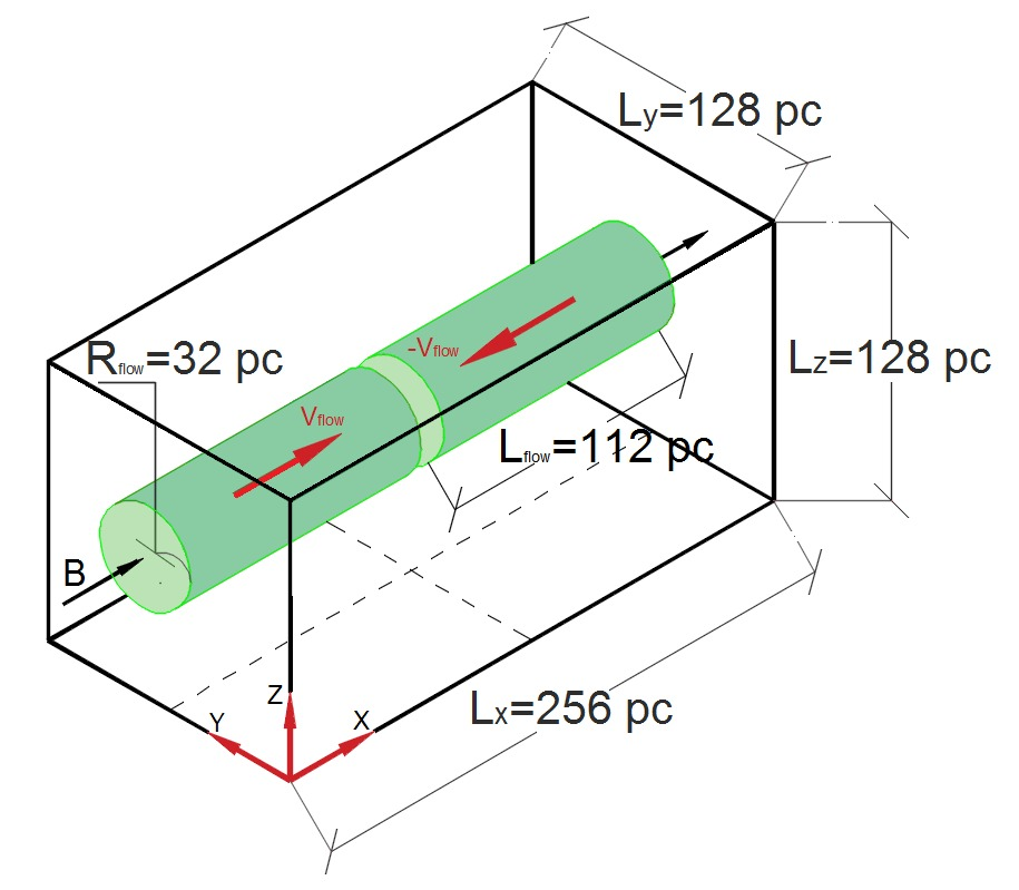
Figure 1: Sketch illustrating the initial conditions used in this work, which consist of two cylindrical streams colliding at the centre of the numerical box. Figure adapted from Körtgen & Banerjee (2015).

2.5 Initial conditions

We use the setup pictured in Fig. 1 for the initial conditions, which are as follows. The numerical periodic box, of sizes $L_{x}=256\,{\rm pc}$ and $L_{y}=L_{z}=128\,{\rm pc}$, is initially filled with warm neutral gas at uniform density of $2\,{\rm cm}^{-3}$ and constant temperature of $1450\,{\rm K}$.

We impose an initial background velocity field, which corresponds to a moderate turbulence with a power spectrum of $k^{-2}$ and Mach number of $\mathcal{M}_{\rm rms}\simeq 0.7$, whose main role is to trigger instabilities in the converging-flow we set up on top of this random field. This setup consists of two cylindrical streams entirely contained in the numerical domain (see Fig. 1), each of radius $R_{\rm flow}=32\,{\rm pc}$ and length $L_{\rm flow}=112\,{\rm pc}$, moving in opposite directions at a moderately supersonic velocity of $v_{\rm flow}=7.5\,{\rm km~{}s}^{-1}$ in the $x$-direction. Thus, the inflow Mach number is $\mathcal{M}_{\rm flow}=2.42$ and the corresponding dynamical time is $t_{\rm dyn}=L_{\rm flow}/v_{\rm flow}=14.6$ Myr. Note that the gas mass in the whole box is $\sim 2.6\times 10^{5}\,M_{\odot}$, whereas the mass contained in the cylinders is $\sim 4.5\times 10^{4}\,M_{\odot}$ (assuming a mean molecular weight $\mu=1.27$).

The numerical box is permeated by a uniform magnetic field of $3\,\mu\mathrm{G}$ along the $x$-direction. Thus, the corresponding mass-to-flux ratio in the cylinders is $1.59$ times the critical value, so that the cloud formed by the colliding flows eventually will become magnetically supercritical once it accrete enough mass. The initial plasma beta parameter (i.e., the thermal to magnetic pressure ratio) is $\beta_{\rm th}\equiv P_{\rm th}/P_{\rm mag}\simeq 1.1$ and the Alfvén mach number $\mathcal{M}_{\rm A}=1.3$. We achieve a maximum resolution of $\Delta=0.03\,{\rm pc}$ in all the three dimensions.

With this setup we ran model B3 in Paper I (Feedback-Off model hereafter). In this work, we restart this simulation to include ionising feedback from the point when the first massive star appears ($t\sim 12.8\,{\rm Myr}$; model Feedback-On hereafter) and let it evolve for $\sim$6 Myr more. This period is long enough to study the evolution of individual Hii regions as well as the global feedback effects on the parent MC.

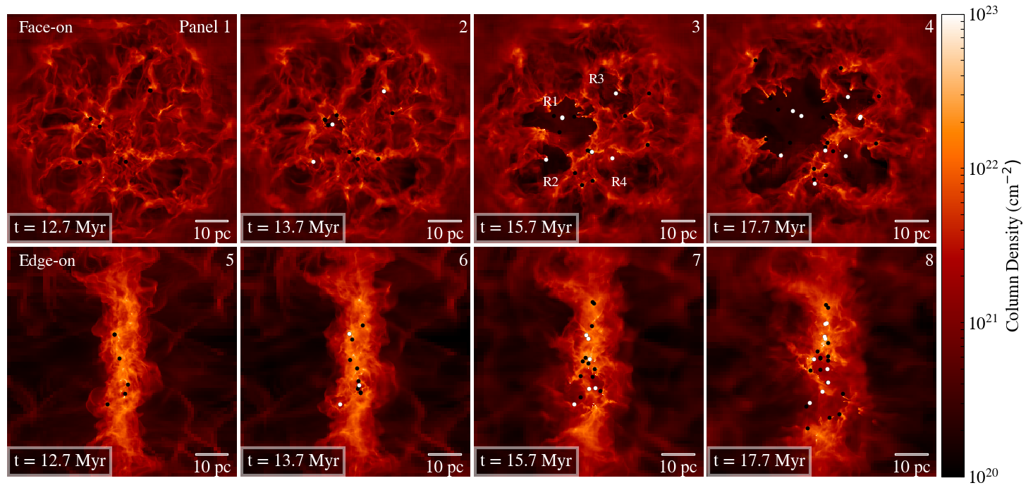
Figure 2: Column density maps in evolutionary sequence for the “central cloud” in the simulation with feedback (Feedback-On model). The upper and lower panels show face-on and edge-on views, respectively. The dots represent the projected position of the sink particles, where the white ones host massive stars. In panel 3 we annotate the name of the four Hii regions we analyse in Sec. 3.2. The projections correspond to the 80 pc central sub-box. See an animation of this figure in the supplementary material.

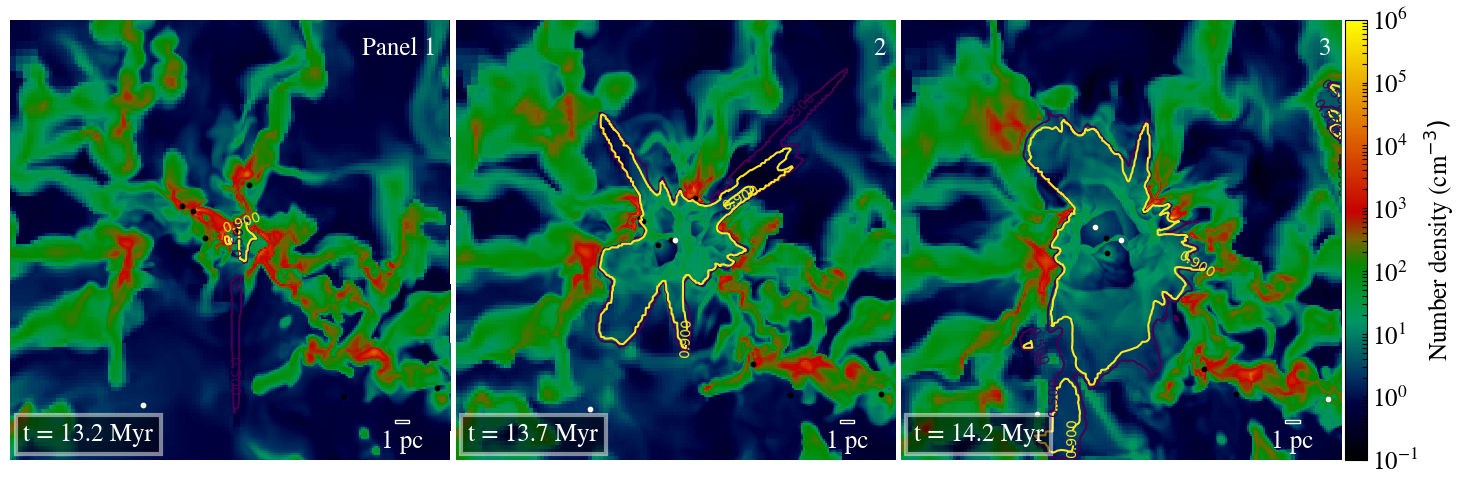
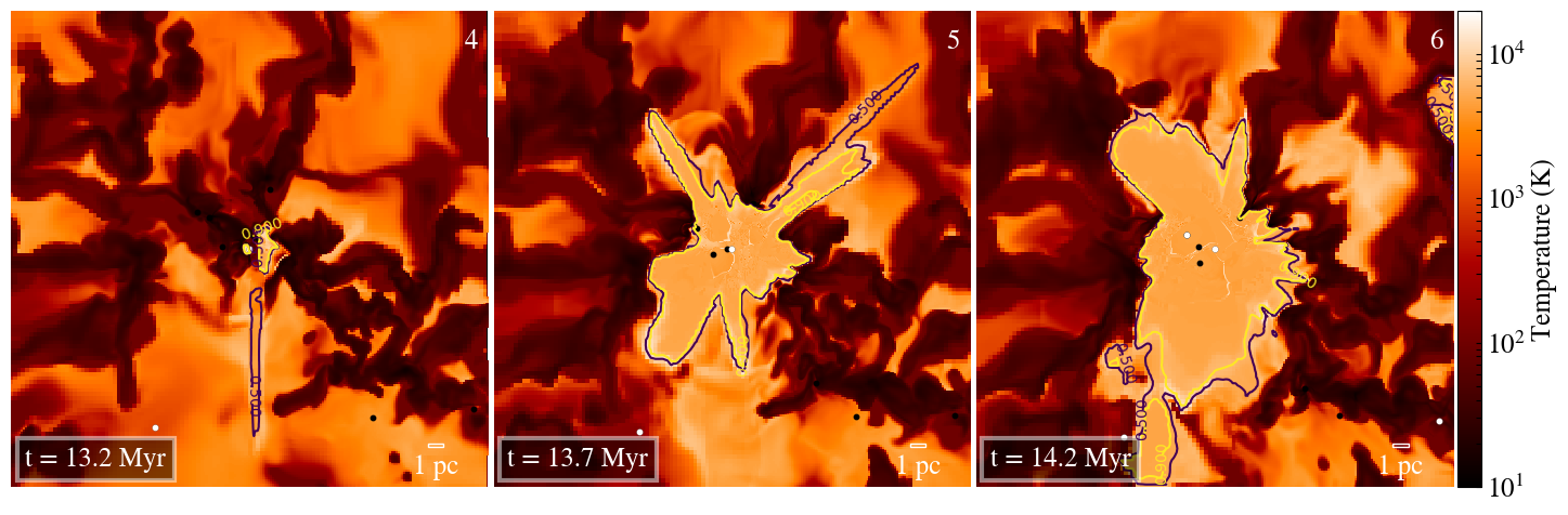
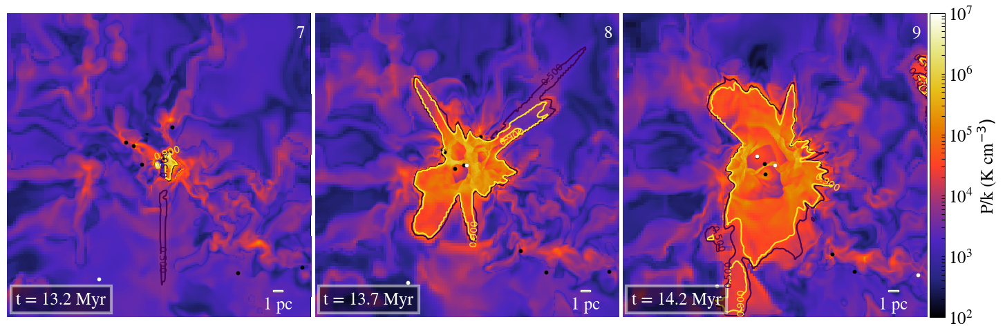
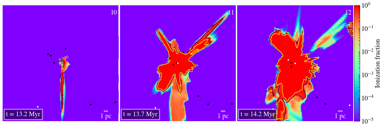
Figure 3: Slices of the number density, temperature, pressure, and ionisation fraction (from top to bottom rows) in the $y-z$ plane (face-on view) for the first Hii region (R1) at different times. Each slice is 30 pc wide and is centred at the position of the massive star. The contours in all panels delineate ionisation fractions of 0.5 (purple) and 0.9 (yellow).

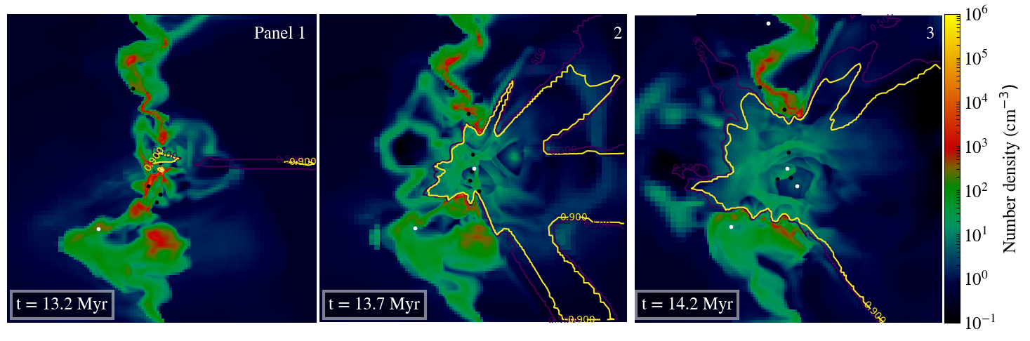
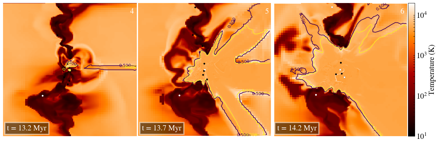
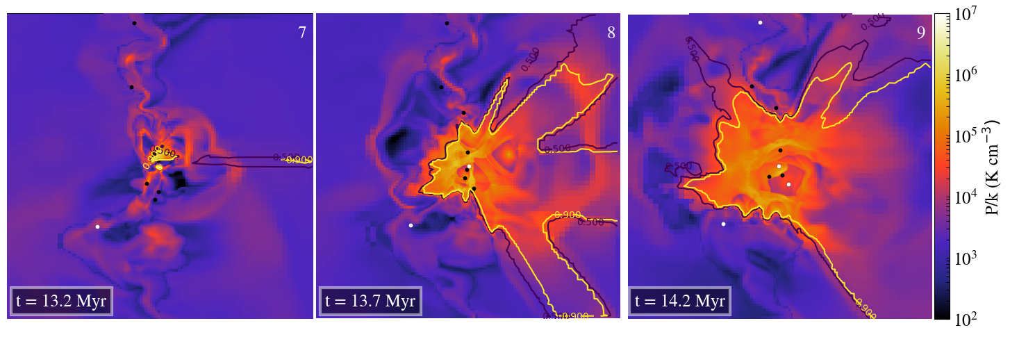
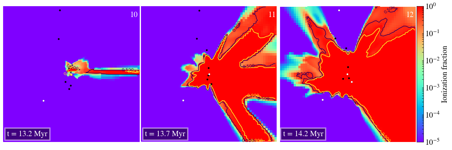
Figure 4: Same as Fig. 3 but in the $x-y$ plane (edge-on view).

3 Results

Henceforth, we focus our discussion on the simulation with feedback (model Feedback-On). For a detailed description about the formation and evolution of the control simulation (model Feedback-Off) we refer the reader to Paper I.

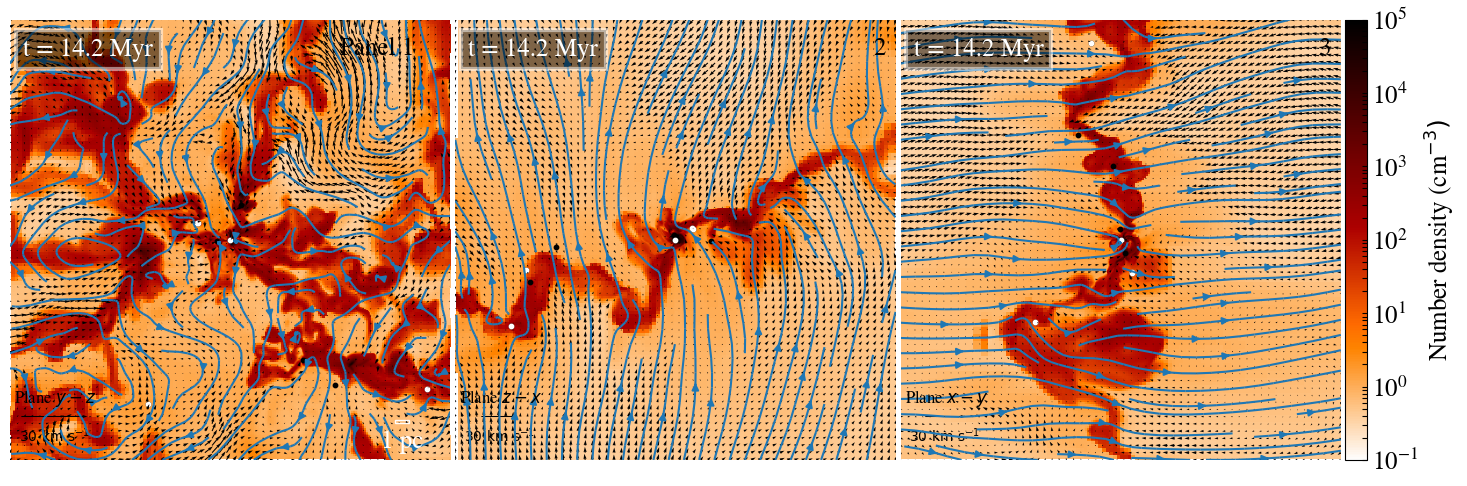
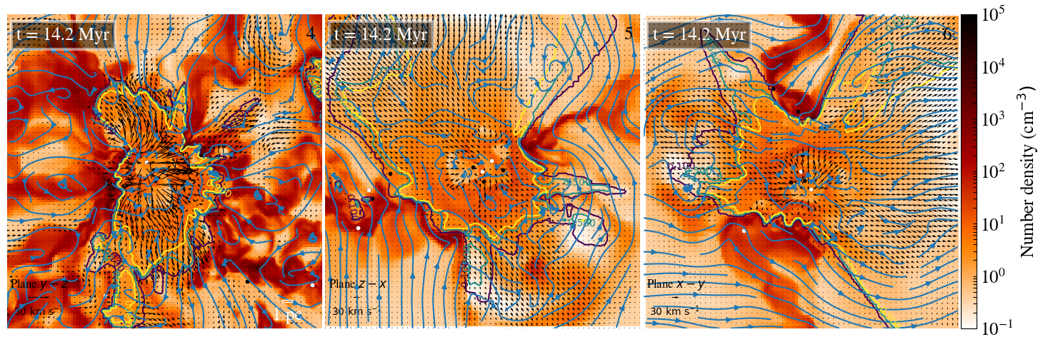
Figure 5: Number density slices of the region “R1” at $t=14.2\,{\rm Myr}$ in the three main projections, $x$, $y$, and $z$ (left, middle, and right panels, respectively). The upper/lower panels correspond to the simulation without/with feedback (i.e., Feedback-Off/Feedback-On models). The black arrows represent the projected velocity field (the vector scale is in the bottom left corner). Blue lines represent magnetic field streamlines. In the lower panels (Feedback-On model), the yellow, light-blue, and purple contours correspond to ionising fractions of 0.9, 0.5, and 0.1, respectively.

3.1 Global evolution

In general, the clouds formed in our colliding flows simulations start as a thin cylindrical sheet of cold atomic gas produced by the thermal instability (see, e.g., Hennebelle & Pérault, 1999; Koyama & Inutsuka, 2000, 2002; Walder & Folini, 2000; Vázquez-Semadeni et al., 2006). The inflows naturally inject turbulence to the cloud through various dynamical instabilities (see, e.g., Hunter et al., 1986; Vishniac, 1994; Koyama & Inutsuka, 2002; Heitsch et al., 2005; Vázquez-Semadeni et al., 2006). The cloud continues accumulating mass via accretion and eventually becomes gravitationally unstable and begins to contract gravitationally, entering a regime of hierarchical, multi-scale collapse (Hartmann et al., 2001; Heitsch & Hartmann, 2008; Vázquez-Semadeni et al., 2009; Vázquez-Semadeni et al., 2019). Some time after that ($t\sim 11.6\,{\rm Myr}$), star formation begins in the densest fragments (clumps), while these fragments continue to fall towards the global centre of mass. The first radiating sink forms at $t\sim 11.8\,{\rm Myr}$ (with a mass of $\sim 3.5\,M_{\odot}$) and starts to radiate at $t\sim 12.8\,{\rm Myr}$ once it accretes enough mass to host a massive star, according to our subgrid SF prescription (see 2.2).

In Fig. 2 we show the column density structure of the simulation with feedback in face/edge-on projections at different time steps (see the corresponding movie in the supplementary material). Note the highly complex filamentary structure of the dense gas (especially at $t\sim 12.7\,{\rm Myr}$), which is a common feature in observed molecular clouds (see, e.g. André et al., 2013, and references therein) and simulations (e.g, Gómez & Vázquez-Semadeni, 2014; Smith et al., 2014; Zamora-Avilés et al., 2017). At later times ($t\sim 15.7{\rm Myr}$) the effect of ionising feedback is evident and we can see the features typical of Hii regions, such as pillars, elephant trunks, and champagne flows (see, e.g., Hester et al., 1996). In Figs. 3 and 4 we show slices of the number density, temperature, pressure, and ionisation fraction for the first Hii region that appears (region labeled “R1” in panel 3 of Fig. 2) in two different projections and for three different early times ($t=13.2$, 13.7, and 14.2 Myr). It is worth noting that the HII regions in these filamentary structures immersed in a WNM are far from spherical and properties such as size are strongly projection-dependent.

In Fig. 5 we show 30-pc slices at $t=14.2$ Myr centred at the position of the first massive star that appears for the simulations without and with feedback (upper and lower panels, respectively). The left, middle and right panels correspond to slices in planes $y-z$, $z-x$, and $x-y$, respectively. The first feature worth noting in the simulation without feedback (upper panels) is that the filament containing the massive star is perpendicular to the magnetic field lines (see blue streamlines in panels 2 and 3; see also Gómez et al., 2018). This is probably a consequence of the initial conditions, however, it could be also the result of the magnetic field being oriented by the accretion flow from the cloud onto the filament (e.g., Zamora-Avilés et al., 2017), rather than the field guiding the flow, as such morphology is often interpreted.

In contrast, in the simulation with feedback, the ionised gas is over-pressured and escapes in a champagne flow to the WNM at velocities of tens of ${\rm km~{}s}^{-1}$ (see panels 5 and 6 in Fig. 5). Note that in the nearest 10 pc around the massive star, the magnetic field lines are highly disorganised. However, beyond that distance, the magnetic field is quite ordered and tends to be aligned with the velocity field of the outflowing gas. This outflowing material is mostly composed of fully ionised gas, as the ionisation fraction contours show in panels 4-6 of Fig. 5 (purple, light-blue, and yellow contours denote ionisation fractions of 0.1, 0.5, and 0.9, respectively). Although we have been discussing mostly the morphology and dynamics of region R1 (see panel 3 of Fig. 2), the other regions have quite similar characteristics.

Finally, it is worth mentioning that magnetic fields may play only a minor role in the evolution of Hii regions since the ram pressure dominates the dynamics of the ionised gas, as was found by Arthur et al. (2011). However, magnetic fields are probably important for the dense gas surrounding Hii regions, but this investigation is beyond the scope of this study (see, e.g., Krumholz & Federrath, 2019).

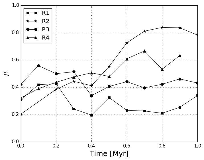
Figure 6: Evolution of the ratio of minimum and maximum axes ($\mu$) for each region. Lower values of this ratio mean regions highly anisotropic, while values tending to one correspond to more symmetric regions.

Table 1: Properties of the analysed Hii regions (see panel 3 of Fig. 2). Here, $t_{0}$ is the time at which each massive star, of mass $M_{*}$, starts radiating; $R$, $\langle n\rangle$, $M_{\rm I}$, and $v_{\rm rms}$ are the radius, mean density, ionised gas mass, and velocity dispersion of each Hii region after $\sim 1\,{\rm Myr}$ of evolution.

Region	$M_{*}$a	$t_{0}$	$R$	$\langle n\rangle$	$M_{\rm I}$	$v_{\rm rms}$
name	$(M_{\odot})$	(${\rm Myr}$)	(pc)	(${\rm cm}^{-3}$)	($M_{\odot}$)	(${\rm km~{}s}^{-1}$)
R1	15.2	12.8	14.5	0.9	358.5	11.2
R2	10.1	13.1	3.2	5.3	23.6	14.8
R3	9.9	13.4	3.8	2.5	17.4	16.0
R4	12.7	14.3	3.7	8.5	38.1	12.4

• Note that a once massive stars reach $8\,M_{\odot}$ it starts to radiate. However, the radiation does not stop the mass accretion immediately and the mass of the sink/massive star continue growing.

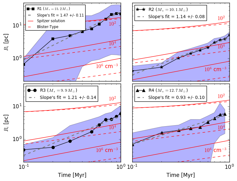
Figure 7: Time evolution of the radii of the four Hii regions marked in panel 3 of Fig. 2. Grey dashed lines represent the best power-law fit (the slopes are in the figure label). The solid red lines correspond to the classical Spitzer solution (eq. (14) in the Appendix) for expanding Hii regions immersed in a uniform medium of density $10^{6}$, $10^{4}$, and $10^{2}\,{\rm cm}^{-3}$, respectively, whereas the dashed red lines trace the blister-type solution (Eq. (9) in FST94; see also eq. (10) in the Appendix), assuming the same cloud densities that in the Spitzer solution. Finally, The blue-shaded region represents the size range between the extremes of the distance between the star and the ionisation front for each region.

3.2 Evolution of the Hii regions

We define an Hii region around a massive star as the connected region around the ionising source where the ionisation fraction is greater than 0.5. We then calculate the evolutionary properties of individual Hii regions as long as they remain isolated and powered by a single massive star, which corresponds to roughly 1 Myr. After this time, the regions merge with each other or another massive star appears. Thus, we study four Hii regions, which are marked in panel 3 of Fig. 2 as R1, R2, R3, and R4. In Table 1 we list the main properties of these regions after $\sim 1$ Myr of evolution.

Here, we focus our discussion in the size, density, and mass of our selected regions, since other physical properties, such as temperature, velocity dispersion, and rms magnetic field strength remain roughly constant around the mean values of $10^{4}$ K, $12\,{\rm km~{}s}^{-1}$, and $1\,\mu$G, respectively, for all regions.

We also quantify the anisotropy level by computing the size of the three principal axis. First we calculate the inertia matrix $I_{i,j}=\sum x_{i}x_{j}\Delta m$, where $x_{i}$ and $x_{j}$ are the coordinates to every cell belonging to the Hii region. We then calculate the eigenvectors of the inertia matrix, $I_{i}$, which represent the inertia momentum. The principal axes can be calculated as $\mu_{i}=\sqrt{I_{i}/M_{i}}$, where $M_{i}$ is the ionised mass. In Fig. 6 we plot the ratio of minimum and maximum axes ($\mu=\mu_{3})/\mu_{1}$), and we can see that in general our regions grow anisotropically (with $\mu\lesssim 0.6$), except for the second Hii region (star symbols), which tends to be more symmetric after $\sim 0.5$ Myr of evolution.

3.2.1 Size

With the above definition of an Hii region, and in order to estimate a characteristic size of the Hii regions, we first calculate the total volume ($V$) and then calculate the radius as $R_{\rm i}=V^{1/3}$. In Fig. 7 we show the evolution of the radius of our four Hii regions. We have chosen the zero of time as the moment when each massive star starts to radiate ($t_{0}$ in Table 1).

In the same figure, we have over-plotted the Spitzer solution as well as the blister-type (FST94) estimation for the radius evolution of blister-type HII regions (solid and dashed red lines, respectively; see Appendix A). Note that both the Spitzer and the FST94 solutions describe only the growth of the cavity within the dense cloud, while our calculations include the ionised gas that escapes into the diffuse intercloud medium. Thus, the analytic solutions should be considered only as guidelines. The actual flow is more similar to the “champagne” flow described by Franco et al. (1990), although without a unique expansion law because our cloud is filamentary and highly irregular rather than exhibiting a smooth stratification as assumed by those authors.

Also, in Fig. 7, the blue-shaded regions represent the size range between the minimum and maximum values of the distance between the star and the ionisation front for the four Hii regions studied. It is worth noting that the minimum values of this star-front distance occur in the direction toward the densest parts of the cloud (see, for example, panel 1 in Fig. 3). In this direction, the ionisation front remains stationary, and very close to the star ($R_{\rm i}\la 0.1$ pc) for most of the time interval considered in three out of the four Hii regions we analysed. This imply that the simulated Hii regions grow anisotropically, and thus the stars appear off-centre of the regions during their evolution.

In Fig. 7 we also show grey dashed lines that represent the best power-law fit to the mean radius of the regions, $R_{\rm i}$, as a function of time. We find that $R_{\rm i}\propto t^{1.18\pm 0.17}$, where the uncertainty range represents the standard deviation among our four regions. This implies that the expansion velocity and acceleration are proportional to $\sim t^{0.2}$ and $\sim t^{-0.8}$, respectively. Thus, once an ionised region breaks out from its host filament, a blister-type flow is generated which expands in an accelerated way towards the low density parts of the MC and the diffuse medium. This accelerated behaviour has been reported by Franco et al. (1990) and Arthur & Hoare (2006) for Hii regions expanding in a stratified medium.

3.2.2 Density

The left panel of Fig. 8 shows the mean density, $\langle n_{i}\rangle$, as a function of time of the ionised gas. The initial density is high $\gtrsim 10^{3-4}\,{\rm cm}^{-3}$, but the Hii regions deflate quickly as they reach (and expand through) the WNM, lowering their density by roughly three orders of magnitude after $\sim$1 Myr of evolution. The final density for all the regions tends to saturate around $\sim 1-5\,{\rm cm}^{-3}$.

3.2.3 Mass

As expected, the ionised mass, $M_{i}$, of the Hii regions depends on the mass and luminosity of the ionising star (see Fig. 8; right panel). Region R1 is produced by the most massive star in our sample ($15.2\,M_{\odot}$; see Table 1), and it ionises a gas mass of $~{}400\,M_{\odot}$, whereas the stars with masses around $~{}10\,M_{\odot}$ (regions R2 and R3) only ionise $\sim 20\,M_{\odot}$ after $\sim 1\,{\rm Myr}$.

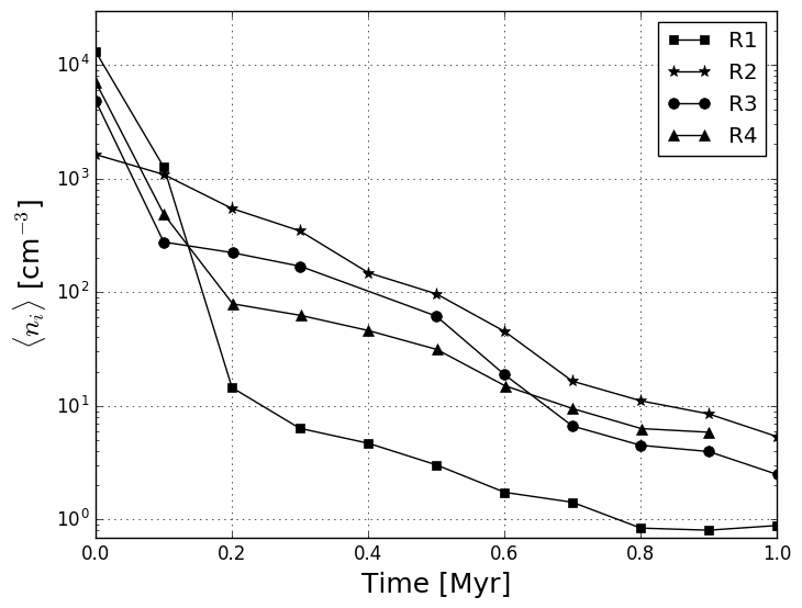
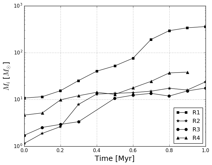
Figure 8: Time evolution of the mean number density of ionised gas (left panel) and ionised gas mass (right panel) for the four Hii regions.

3.2.4 The size-density relation

As mentioned in the introduction, Hii regions observationally show a clear correlation between size ($R_{\rm i}$) and the electronic density ($n_{i}$) of the form $n_{i}\propto R_{\rm i}^{p}$, with $p\simeq-1$, over a wide dynamical range (see, e.g., Hunt & Hirashita, 2009), although with a considerable dispersion of $\sim 2$ orders of magnitude. Figure 9 shows our Hii regions in this size-density diagram. We find a tight correlation, although with a steeper slope, $p\simeq-2$, for all our Hii regions throughout their evolution. Some possible explanations for this discrepancy in the slope are the lack of other feedback mechanisms (winds and supernova) in our models, or the fact that our Hii regions are produced for a single massive star, whereas probably most of the regions in the Hunt & Hirashita (2009) sample contain more than one OB star.

Note also that, although both the evolution of the size and density depend on the mass of the ionising star, the density-size relations do not. Indeed, all the Hii regions are seen to occupy the same region in this diagram (see Fig. 9). This suggests that the position of a given Hii region in this diagram can be explained in terms of its evolutionary state alone. On the other hand, this relation also implies that the mass of the Hii regions roughly depends linearly on their size; that is, $M_{i}\propto R_{\rm i}$, assuming constant density.

Figure 9: Size-density diagram for the four simulated Hii Regions. The blue shadow brackets the radius extremes for the region R1 at each time (see upper-left panel of Fig. 7). The average of the slopes is 2.0, i.e., $n_{i}\propto R_{\rm i}^{-2}$. The red symbols correspond to the time at which each Hii region turns on (at higher density and smaller sizes).

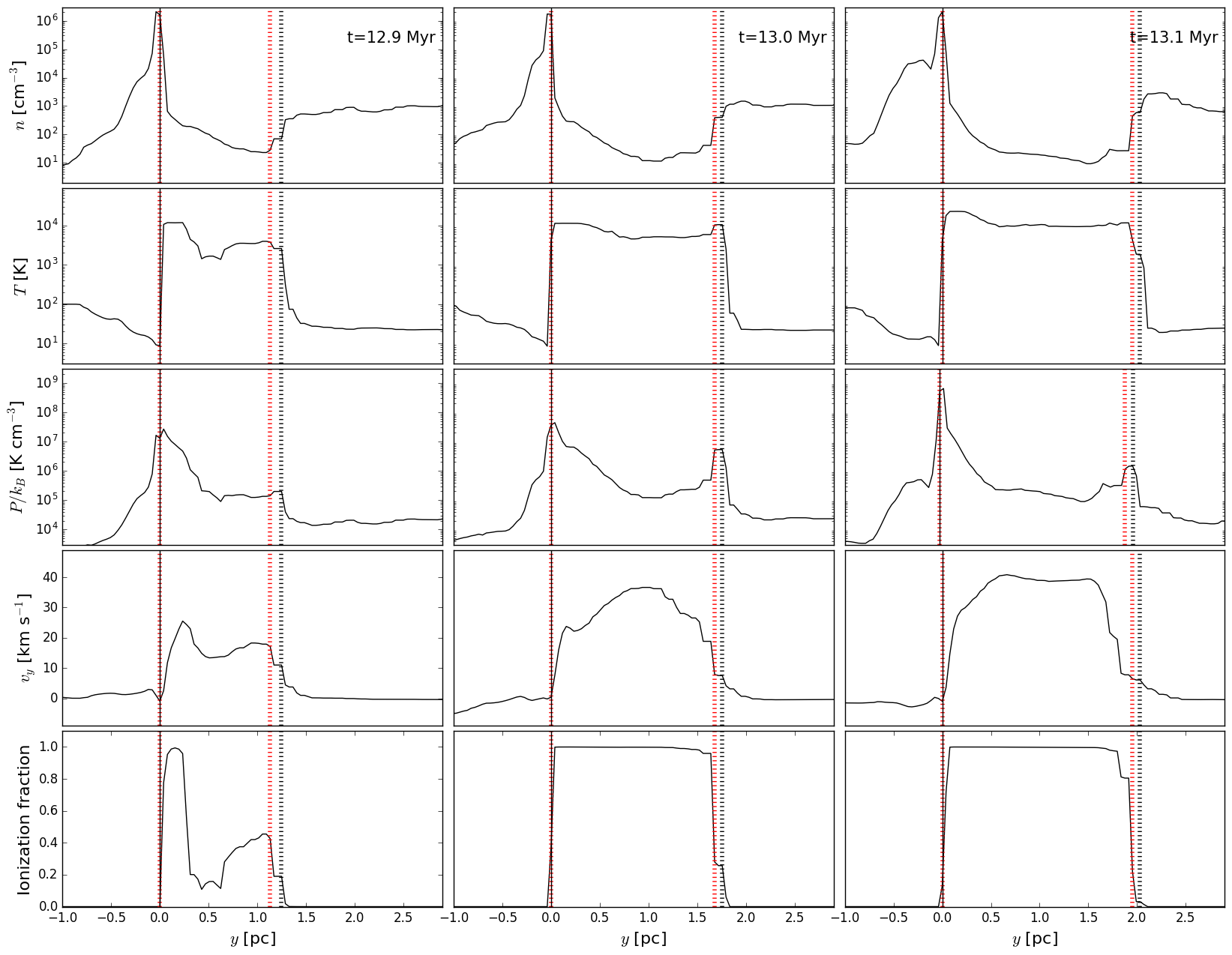
Figure 10: Density, temperature, pressure, velocity, and ionisation fraction profiles (from top to bottom) for the R1 in the $y$-axis at times 12.9, 13, and 13.1 Myrs (left, middle, and right panels, respectively). The zero point corresponds to the position of the massive star (vertical thin black line). The dotted black and red vertical lines represent the shock and ionisation fronts, respectively.

4 Structure of the Hii regions

Our simulations, including a physically reasonable treatment of the radiative transfer, provide an ideal means for investigating the structure of the Hii regions and their boundaries, especially since there exist various models in the literature for the expansion of these regions which are based on different assumptions of their boundary conditions and internal structure.

The expansion of Hii regions into their parent MCs depends on whether they are fully embedded in the MC, constituting the “canonical” Hii regions (e.g., Spitzer, 1978), or break out of the dense clouds and begin expanding into the diffuse medium, constituting the so-called “blister” type of Hii regions (e.g., Whitworth (1979); Franco et al. (1990); FST94). As summarised in Appendix A, during their dynamical expansion phase, canonical Hii regions are overpressured relative to the cloud material, and are therefore bounded by a shock front, followed downstream by an ionisation front, with a shocked, dense layer in between the two fronts. Furthermore, as a consequence of the overpressure in the region and the dynamical expansion it produces, which reduces the region’s internal density, the region follows an expansion law of the form $R\sim t^{4/7}$.

Instead, blister-type regions are characterised by a loss of pressure by means of the “release valve” provided by the discharge to the diffuse medium. Therefore, FST94 argued that these regions are essentially at the same pressure as their parent cloud and thus do not produce a shock front upstream of the ionisation front. This in turn implies that the region is bounded, on its interface with the cloud, by a single ionisation front, with no preceding shock front and no compressed neutral layer upstream of it. Also, because in this case the region is not overpressured, its growth is controlled only by the rate at which the mass inflow through the ionisation front balances the mass loss to the diffuse medium (see Fig. 1 of FST94), resulting in a slower expansion rate into the cloud of the form $R\sim t^{2/5}$.

This conclusion, together with the associated mass photo-evaporation rate of the cloud predicted by FST94 has been questioned by Matzner & Jumper (2015), who argue that FST94 “incorrectly associate swept-up mass with ionised mass.” This is because, according to Matzner (2002), most of the mass in the Hii region is in the shocked, compressed layer upstream of the ionisation front. Moreover, the criticism by Matzner & Jumper (2015) indirectly affects the accuracy of a model we have presented in previous papers for the collapse of MCs and their SF activity (Zamora-Avilés et al., 2012; Zamora-Avilés & Vázquez-Semadeni, 2014), which was based on the prescription by FST94. However, this criticism only applies if blister Hii regions develop a shock at the interface with the MC. If no shock is present, then there is no swept-up, dense layer, and so all the material in the region is indeed ionised.

Our results, described in the previous sections, allow us to investigate what is the actual nature of the boundary between the Hii region and the cloud, since the radiative transfer and the cooling rates are followed self-consistently, and thus the ionisation fraction and the gas structure are realistic, including the presence and position of the ionisation front and the shock. In Figs. 3 and 4 we show the contours where the ionisation fraction $\chi=0.5$ (purple) and $\chi=0.9$ (yellow) in region R1. In the top panels these contours are overlaid onto images of the density, while in the second and third rows they are overlaid onto images of the temperature and the pressure, respectively.

The signature of a shock ahead of the ionisation front should be a region of high density and pressure between the ionisation front and the ionised region, with a higher temperature than that of the cloud. In order to detect shocks in our simulated Hii regions, we plot in Fig. 10 profiles of the density, temperature, pressure, velocity ($y$-component), and ionization fraction for the R1 and for three different times in the frame of reference of the massive star. No evidence of a shock upstream of the ionization front is seen at the edges of the R1 region where it meets with the densest gas, unless it is too weak to be detected. Note that this behaviour (a very weak shock toward the densest part) is also reported by Arthur & Hoare (2006) in a stratified density field.

On the other hand, we detect a clear shock toward the general cloud (marked with vertical dotted black lines in Fig. 10) ahead of the ionisation front (right vertical dotted red lines) due to the hydrodynamical expansion of the Hii region. Thus, our Hii regions expand in a hybrid way: towards the general cloud we detect a moderate shock, whereas we do not detect any shock signature (or it is too weak to be detected) toward the dense clump.

Furthermore, this region also exhibits features of the blister type, as it has ample sections where it connects directly to the warm, diffuse gas. In these sections, it expands in an accelerated manner, in qualitative agreement with the analytical predictions of Franco et al. (1990), although, due to the non-unique density stratification, our region does not exhibit a unique acceleration law. Thus, we conclude that neither the classical $t^{4/7}$ nor the FST94 $t^{2/5}$ expansion laws apply to our regions, which instead expand in an accelerated way as $R_{\rm i}\sim t^{1.2}$, in qualitative agreement with Franco et al. (1990).

5 Discussion

5.1 Implications of the size-density relation

Hunt & Hirashita (2009) interpreted the observed size-density relation for Hii regions ($n_{i}\propto R_{\rm i}^{-1}$) as being a consequence of the observed Larson relation for molecular clouds ($n_{H_{2}}\propto R_{H_{2}}^{-1}$), suggesting that Hii regions retain an imprint from the molecular environment in which they form. However, this Larson relation has been repeatedly questioned, since it may be the result of various selection effects, rather than real property of MCs (e.g., Kegel, 1989; Scalo, 1990; Vázquez-Semadeni et al., 1997; Ballesteros-Paredes & Mac Low, 2002; Ballesteros-Paredes et al., 2012). Indeed, numerical simulations of MC formation and evolution do not show any evidence for the appearance of such a density-size scaling appearing in the clouds unless a selection criterion of roughly constant column density is imposed (Ballesteros-Paredes & Mac Low, 2002; Camacho et al., 2016). On the other hand, our results strongly suggest that individual Hii regions do follow an evolutionary path in the $n_{i}-R_{\rm i}$ diagram. This evidence suggests that, the size-density scaling of Hii regions may be a real effect, although, contrary to the interpretation of Hunt & Hirashita (2009), unrelated to the density structure of the parent MC.

5.2 Comparison with previous results

Analytical models of blister-type expansion of Hii regions are based on different hypotheses. While FST94 assume that the ionization front advances with no shock towards the dense region of the cloud, Matzner (2002) assumes that it is through this shock that the Hii region incorporates most of its mass (see App. A). However, in the present study we have shown that both of these hypotheses are satisfied at the same time in different parts of the Hii regions. The assumption by FST94 is valid toward the dense gas (where the massive star was born), while the assumption of Matzner (2002) can be applied toward the rest of the cloud. On the other hand, the Hii regions we analysed expand in an accelerated way toward the low density gas (WNM) as predicted by Franco et al. (1990) in a stratified medium (see also Arthur & Hoare, 2006).

Although the structure and dynamics of massive star-forming regions are quite complicated and far from the idealised geometries assumed in analytical models, an approximate comparison is possible. The size-density relation ($n_{i}\propto R_{\rm i}^{-2.0}$) implies that the ionised gas mass, $M_{i}\propto R_{\rm i}$, or equivalently, $\dot{M}_{i}\propto\dot{R_{\rm i}}$. As we found in §3.2, the Hii region radius depends roughly on time as $R_{\rm i}\propto t^{1.19}$. Therefore, the mass ionisation rate is $\dot{M}_{i}\propto t^{0.19}$. Note that this dependence is quite close to $\dot{M}_{i}\propto t^{1/5}$ predicted by FST94 (Eq. 11) for blister type Hii regions. In turn, this implies that the blister-Hii region approximation used in the analytical model by Zamora-Avilés et al. (2012) is justified.

On the numerical side, several works have included ionising feedback (e.g., Dale et al., 2005; Colín et al., 2013; Geen et al., 2015), although they only study global properties of MCs, rather than the internal structure of the Hii regions. On pc scales, Arthur et al. (2011) studied the evolution of individual Hii regions, albeit only during the embedded phase, so we cannot compare directly our findings with these works. In any case, they showed that the presence of a magnetic field does not modify the Hii region structure in a fundamental way. Finally, although we have investigated only one simulation, our results can be considered robust since our simulated MC is highly chaotic, due to the turbulence injected in a self-consistent way, and therefore the idealised initial conditions are quickly forgotten. Moreover, we have investigated a sample of four Hii regions that span a range of behaviours, from which we have extracted some meaningful averages.

5.3 Limitations

As we are interested in studying the effect of the ionising feedback, in this study we have neglected other feedback processes, such as winds, supernova explosions and radiation pressure, which can help disperse the cloud and further reduce both the SFR and the SFE. However, these feedback effects can also enhance the positive feedback through the injection of mechanical energy, and can possibly bring the slope of the size-density relation of our Hii regions closer to the observed value. Thus, the net effect of these feedback mechanisms is so far unclear, and more numerical research is necessary in order to study their relative importance (see, e.g., Körtgen et al., 2016; Wareing et al., 2017).

Also, our spatial and temporal output resolutions are insufficient to resolve the stages of hyper-compact/compact Hii regions. Particularly, we do not resolve the initial Strömgren radius in our star formation regions. However, this is not an issue since we are interested in studying the expansion of Hii regions at the scale of the MCs, as a means of destroying them. Although our numerical simulations include magnetic fields, it is still necessary to assess its detailed influence on the feedback processes through comparison with non-magnetic simulations, a task we defer to a future contribution.

Finally, the FLASH radiative transport module does not take into account the absorption of UV photons by dust grains inside the Hii regions. Also, models by Hosokawa & Omukai (2009) suggest that the ZAMS model we use can overestimate the ionising luminosity. Both effects tend to overestimate the number of UV photons emitted by a massive star, so properties of Hii regions such as size should be taken as upper limits (see Peters et al., 2010, for a detailed discussion). However, the power law index of the radius growth should remain unchanged, as well as their associated relations. In addition, the effects of molecular hydrogen destruction by photodissociation from massive and intermediate-mass stars is not considered here, and, as discussed by Diaz-Miller et al. (1998), this effect makes the cloud evaporation process more effective.

6 Summary and Conclusions

In this paper, we have studied the evolution of the physical properties of Hii regions in radiation-MHD simulations of MCs formed by diffuse converging flows in the presence of magnetic fields and massive-star ionisation feedback.

Our simulations reproduce the rich morphology observed around Hii regions, such as elephant trunks, cloudlets, champagne flows, etc. Due to the highly complex structure of our filamentary clouds, the Hii regions grow anisotropically, causing the massive stars to appear off-centre of the ionised regions. Our simulated Hii regions expand in a hybrid way in our filamentary clouds: towards the intermediate-density regions in the cloud, the Hii regions expand according to the classical theory, developing a shock ahead of the ionisation front, while towards the densest parts of the cloud, no shock is apparent, and the ionisation front stalls in 3 out of 4 cases, and advances according to classical theory in the other case. Finally, towards the diffuse, warm gas, the regions expand roughly according to the “blister” case, at an accelerated pace. On average, the radius of the regions is dominated by this latter mode, so that the average radius grows at an accelerated pace, roughly as $R_{\rm i}\sim t^{1.2}$.

Our Hii regions exhibit a tight relation between size and average density, $\langle n_{i}\rangle$, of the form $\langle n_{i}\rangle\propto R_{\rm i}^{-2}$. This implies that, on average, the mass ionisation rate is $\dot{M}_{i}\propto t^{0.19}$, which is in good agreement with the analytical prediction by FST94 ($\dot{M}_{i}\propto t^{0.2}$). Therefore, we conclude that the analytic prescription for the rate of mass ionisation used in the model by Zamora-Avilés et al. (2012) is adequate, contrary to Matzner & Jumper (2015). Interestingly, the electron density-size relation we observe in our Hii regions is the result of the expansion mechanism itself, rather than an imprint of a Larson-type relation in their environment, which, in addition, is not observed in general in this kind of simulations.

Appendix A Dynamical evolution of Hii regions

The different phases of the evolution of an Hii region have been studied in several previous works (see, e.g., Spitzer, 1978; Whitworth, 1979; Dyson & Williams, 1980) At first, a Hii region expands until the ionisation balance is reached, when the ionisation front is located at the initial Strömgren radius $R_{0}$. Afterwards, the Hii region enters into a second stage of dynamical evolution as long as the ionised gas has a higher pressure than the neutral ambient medium. In the particular case of a massive star located near the surface of a molecular cloud, the Hii region is radiation-bounded on the inner part of the cloud, and density-bounded on the outer part (e.g., Whitworth, 1979). Consequently, a cometary Hii region is produced, in which the ionised gas flows into the low-density medium.

FST94 estimated the maximum number of massive stars that can form within a molecular cloud. These authors pointed out that the most efficient destruction mechanism is the evaporation of the cloud by stars located near the cloud’s boundary. In that case, the growth of a Hii region inside the cloud is due to the mass flux (a blister-type mass loss) that expands into the external low-density medium $n_{0}$ at a velocity equal to the sound speed $c_{I}$ in the Hii region. In their model, it is assumed that the mass loss into the environment is equal to the mass gained by the expansion of the Hii region inside the cloud, that is,

$$\pi R_{i}^{2}m_{p}\langle n_{i}\rangle c_{s}=2\pi R_{\rm i}^{2}m_{p}n_{0}\dot{R}_{i}\,,$$ (8)

being $R_{i}$ is the position of the ionisation front, $\langle n_{i}\rangle$ the mean density of the ionised gas, $c_{s}$ the initial expansion speed of the ionised gas into the external low-density medium (which is assumed equal to the sound speed in the ionised gas), and $m_{p}$ the proton mass.

Consequently, the velocity of the ionisation front into the cloud is given by,

$$\dot{R}_{i}\simeq{{\langle n_{i}\rangle}\over{2\,n_{0}}}\,c_{s}\,,$$ (9)

Considering that the total ionised mass remains constant, it follows that the position of the ionisation front at a time $t$ within the cloud is obtained by,

$$R_{i}\simeq R_{0}\,\biggl{(}1+{{5}\over{2}}\,{{c_{s}\,t}\over{R_{0}}}\biggr{)}^{2/5}\,.$$ (10)

For this, these authors neglected the effects of the weak shock of the expanding Hii region due to the mass loss from the blister, and pointed out that both the mass and ionisation balance determines the evolution.

Assuming a constant luminosity during the main-sequence stage of the star, the cloud evaporation rate induced by a single star located near the cloud’s boundary calculated by these authors is given by,

$$\dot{M}_{i}(t)\simeq 2\pi\,R_{0}^{2}m_{p}c_{s}n_{0}\,\biggl{(}1+{{5}\over{2}}\,{{c_{s}\,t}\over{R_{0}}}\biggr{)}^{1/5}\,.$$ (11)

On the other hand, Matzner & Jumper (2015) argued that this photoevaporation rate incorrectly associates the swept-up mass with ionised mass. In another work, Matzner (2002) presented a simple treatment of the momentum generation by an Hii region. This author takes into account the inertia of the dense shell produced by the shock moving into the cloud. In this stage of evolution ($R_{\rm i}>R_{0}$), the expansion of the ionisation front is caused by the pressure gradient between the Hii region and the environment of neutral gas. It is assumed by the author that nearly all of the mass originally located inside the radius $R_{\rm i}$ remains within the shocked shell. According to this author, if the ionised gas is effectively isothermal in blister regions, the ionisation front tends to a D-critical case, for which,

$$u_{II}-\dot{r}_{II}=-c_{II}$$ (12)

where $u_{II}$ is the velocity of the ionised gas relative to the cloud, $\dot{r}_{II}$ is the expansion speed of the ionisation front, and $c_{II}$ is the sound speed of the ionised gas. Consequently, the rate at which mass is ionised is given by,

$$\dot{M}_{II}=\rho_{II}(\dot{r}_{II}-u_{II})\,2\pi r_{II}^{2}\,$$ (13)

where $\rho_{II}$ is the density within the Hii region.

Since the Hii region expands supersonically with respect to the molecular gas, it is bounded by a thin shocked layer that is located near the ionisation front. Assuming a radial expansion, Matzner (2002) found a self-similar solution for $r_{II}\gg R_{\tiny\mbox{St,0}}$ (with $R_{\tiny{\mbox{St,0}}}$ the initial Str$\ddot{\mbox{o}}$mgren radius) given by,

$$r_{II}={{49}\over{6}}\,\,R_{{\tiny\mbox{St,0}}}^{3/7}\,(c_{II}t)^{4/7}$$ (14)

Considering the momentum of the radial motion of the expanding shell, the mass evaporated for a blister region can be estimated by,

$$\delta M_{\tiny{\mbox{d}est}}=1.2\times 10^{4}\,\biggl{(}{t\over{3.7\,{\mbox{M}yr}}}\biggr{)}^{9/7}\biggl{(}{{N_{\tiny{\mbox{H},22}}}\over 1.5}\biggr{)}^{-3/14}$$ (15)

$$\times M_{\tiny\mbox{cl,6}}^{1/14}\,S_{49}^{4/7}{\mbox{M}_{\odot}},$$

where $N_{\tiny{\mbox{H},22}}$ is the mean hydrogen column density in units of $10^{22}$ cm^-2, $M_{\tiny\mbox{cl,6}}$ is the mass of the cloud in units of $10^{6}$ M_⊙, and $S_{49}$ is the ionising photons’ rate in units of $10^{49}$ photons per second. According to this author, equation [15] for the mass evaporated agrees with predictions by Williams & McKee (1997) who argued that only 10$\%$ of the mass of a GMC becomes stellar, within 1$\%$.

References

- André et al. (2013) André P., Di Francesco J., Ward-Thompson D., Inutsuka S.-i., Pudritz R. E., Pineda J., 2013, preprint, (arXiv:1312.6232)
- Arthur & Hoare (2006) Arthur S. J., Hoare M. G., 2006, The Astrophysical Journal Supplement Series, 165, 283
- Arthur et al. (2011) Arthur S. J., Henney W. J., Mellema G., de Colle F., Vázquez-Semadeni E., 2011, MNRAS, 414, 1747
- Ballesteros-Paredes & Mac Low (2002) Ballesteros-Paredes J., Mac Low M.-M., 2002, ApJ, 570, 734
- Ballesteros-Paredes et al. (2011) Ballesteros-Paredes J., Hartmann L. W., Vázquez-Semadeni E., Heitsch F., Zamora-Avilés M. A., 2011, MNRAS, 411, 65
- Ballesteros-Paredes et al. (2012) Ballesteros-Paredes J., D’Alessio P., Hartmann L., 2012, MNRAS, 427, 2562
- Ballesteros-Paredes et al. (2015) Ballesteros-Paredes J., Hartmann L. W., Pérez- Goytia N., Kuznetsova A., 2015, MNRAS, 452, 566
- Bally et al. (1987) Bally J., Langer W. D., Stark A. A., Wilson R. W., 1987, ApJL, 312, L45
- Beck (2001) Beck R., 2001, Space Sci. Rev., 99, 243
- Blitz & Shu (1980) Blitz L., Shu F. H., 1980, ApJ, 238, 148
- Bodenheimer et al. (1979) Bodenheimer P., Tenorio-Tagle G., Yorke H. W., 1979, ApJ, 233, 85
- Buntemeyer et al. (2016) Buntemeyer L., Banerjee R., Peters T., Klassen M., Pudritz R. E., 2016, New Astron., 43, 49
- Burkert & Hartmann (2004) Burkert A., Hartmann L., 2004, ApJ, 616, 288
- Camacho et al. (2016) Camacho V., Vázquez-Semadeni E., Ballesteros-Paredes J., Gómez G. C., Fall S. M., Mata-Chávez M. D., 2016, ApJ, 833, 113
- Colín et al. (2013) Colín P., Vázquez-Semadeni E., Gómez G. C., 2013, MNRAS, 435, 1701
- Csengeri et al. (2011) Csengeri T., Bontemps S., Schneider N., Motte F., Dib S., 2011, A& A, 527, A135
- Dale et al. (2005) Dale J. E., Bonnell I. A., Clarke C. J., Bate M. R., 2005, MNRAS, 358, 291
- Dale et al. (2012) Dale J. E., Ercolano B., Bonnell I. A., 2012, MNRAS, 424, 377
- Dalgarno & McCray (1972) Dalgarno A., McCray R. A., 1972, ARA&A, 10, 375
- Diaz-Miller et al. (1998) Diaz-Miller R. I., Franco J., Shore S. N., 1998, ApJ, 501, 192
- Dopita et al. (2006) Dopita M. A., et al., 2006, ApJ, 639, 788
- Dyson & Williams (1980) Dyson J. E., Williams D. A., 1980, Physics of the interstellar medium
- Elmegreen & Lada (1977) Elmegreen B. G., Lada C. J., 1977, ApJ, 214, 725
- Federrath et al. (2010) Federrath C., Banerjee R., Clark P. C., Klessen R. S., 2010, ApJ, 713, 269
- Franco et al. (1990) Franco J., Tenorio-Tagle G., Bodenheimer P., 1990, ApJ, 349, 126
- Franco et al. (1994) Franco J., Shore S. N., Tenorio-Tagle G., 1994, ApJ, 436, 795
- Frank & Mellema (1994) Frank A., Mellema G., 1994, A& A, 289, 937
- Fryxell et al. (2000) Fryxell B., et al., 2000, ApJS, 131, 273
- Galván-Madrid et al. (2009) Galván-Madrid R., Keto E., Zhang Q., Kurtz S., Rodríguez L. F., Ho P. T. P., 2009, ApJ, 706, 1036
- Garay & Lizano (1999) Garay G., Lizano S., 1999, PASP, 111, 1049
- Geen et al. (2015) Geen S., Hennebelle P., Tremblin P., Rosdahl J., 2015, MNRAS, 454, 4484
- Gilbert & Graham (2007) Gilbert A. M., Graham J. R., 2007, ApJ, 668, 168
- Gómez & Vázquez-Semadeni (2014) Gómez G. C., Vázquez-Semadeni E., 2014, ApJ, 791, 124
- Gómez et al. (2018) Gómez G. C., Vázquez-Semadeni E., Zamora-Avilés M., 2018, MNRAS, p. 1924
- González (2002) González R., 2002, PhD thesis, Universidad Nacional Autónoma de México
- González et al. (2004) González R. F., de Gouveia Dal Pino E. M., Raga A. C., Velázquez P. F., 2004, ApJ, 616, 976
- Hartigan et al. (1987) Hartigan P., Raymond J., Hartmann L., 1987, ApJ, 316, 323
- Hartmann & Burkert (2007) Hartmann L., Burkert A., 2007, ApJ, 654, 988
- Hartmann et al. (2001) Hartmann L., Ballesteros-Paredes J., Bergin E. A., 2001, ApJ, 562, 852
- Hartmann et al. (2012) Hartmann L., Ballesteros-Paredes J., Heitsch F., 2012, MNRAS, 420, 1457
- Heitsch & Hartmann (2008) Heitsch F., Hartmann L., 2008, ApJ, 689, 290
- Heitsch et al. (2005) Heitsch F., Burkert A., Hartmann L. W., Slyz A. D., Devriendt J. E. G., 2005, ApJL, 633, L113
- Hennebelle & Pérault (1999) Hennebelle P., Pérault M., 1999, A& A, 351, 309
- Hester et al. (1996) Hester J. J., et al., 1996, AJ, 111, 2349
- Heyer et al. (2009) Heyer M., Krawczyk C., Duval J., Jackson J. M., 2009, ApJ, 699, 1092
- Hosokawa & Omukai (2009) Hosokawa T., Omukai K., 2009, ApJ, 703, 1810
- Hunt & Hirashita (2009) Hunt L. K., Hirashita H., 2009, A& A, 507, 1327
- Hunter et al. (1986) Hunter Jr. J. H., Sandford II M. T., Whitaker R. W., Klein R. I., 1986, ApJ, 305, 309
- Iliev et al. (2006) Iliev I. T., et al., 2006, MNRAS, 371, 1057
- Juárez et al. (2017) Juárez C., et al., 2017, ApJ, 844, 44
- Kegel (1989) Kegel W. H., 1989, A& A, 225, 517
- Kennicutt (1984) Kennicutt Jr. R. C., 1984, ApJ, 287, 116
- Kim & Koo (2001) Kim K.-T., Koo B.-C., 2001, ApJ, 549, 979
- Körtgen & Banerjee (2015) Körtgen B., Banerjee R., 2015, MNRAS, 451, 3340
- Körtgen et al. (2016) Körtgen B., Seifried D., Banerjee R., Vázquez-Semadeni E., Zamora-Avilés M., 2016, MNRAS, 459, 3460
- Koyama & Inutsuka (2000) Koyama H., Inutsuka S. I., 2000, ApJ, 532, 980
- Koyama & Inutsuka (2002) Koyama H., Inutsuka S. I., 2002, ApJL, 564, L97
- Kroupa (2001) Kroupa P., 2001, MNRAS, 322, 231
- Krumholz & Federrath (2019) Krumholz M. R., Federrath C., 2019, Frontiers in Astronomy and Space Sciences, 6, 7
- Krumholz et al. (2007a) Krumholz M. R., Klein R. I., McKee C. F., 2007a, ApJ, 656, 959
- Krumholz et al. (2007b) Krumholz M. R., Stone J. M., Gardiner T. A., 2007b, ApJ, 671, 518
- Krumholz et al. (2014) Krumholz M. R., et al., 2014, Protostars and Planets VI, pp 243–266
- Mac Low & Klessen (2004) Mac Low M.-M., Klessen R. S., 2004, Reviews of Modern Physics, 76, 125
- Martín-Hernández et al. (2003) Martín-Hernández N. L., van der Hulst J. M., Tielens A. G. G. M., 2003, A& A, 407, 957
- Matzner (2002) Matzner C. D., 2002, ApJ, 566, 302
- Matzner & Jumper (2015) Matzner C. D., Jumper P. H., 2015, ApJ, 815, 68
- Mellema & Lundqvist (2002) Mellema G., Lundqvist P., 2002, A& A, 394, 901
- Myers et al. (1986) Myers P. C., Dame T. M., Thaddeus P., Cohen R. S., Silverberg R. F., Dwek E., Hauser M. G., 1986, ApJ, 301, 398
- Osterbrock (1989) Osterbrock D. E., 1989, Astrophysics of gaseous nebulae and active galactic nuclei
- Paxton (2004) Paxton B., 2004, PASP, 116, 699
- Peretto et al. (2007) Peretto N., Hennebelle P., André P., 2007, A& A, 464, 983
- Peretto et al. (2014) Peretto N., et al., 2014, A& A, 561, A83
- Peters (2009) Peters T., 2009, PhD thesis, University of Heidelberg
- Peters et al. (2010) Peters T., Banerjee R., Klessen R. S., Mac Low M.-M., Galván-Madrid R., Keto E. R., 2010, ApJ, 711, 1017
- Rijkhorst et al. (2006) Rijkhorst E.-J., Plewa T., Dubey A., Mellema G., 2006, A& A, 452, 907
- Scalo (1990) Scalo J., 1990, in Capuzzo-Dolcetta R., Chiosi C., di Fazio A., eds, Astrophysics and Space Science Library Vol. 162, Physical Processes in Fragmentation and Star Formation. pp 151–176
- Schneider et al. (2010) Schneider N., Csengeri T., Bontemps S., Motte F., Simon R., Hennebelle P., Federrath C., Klessen R., 2010, A& A, 520, A49
- Smith et al. (2014) Smith R. J., Glover S. C. O., Klessen R. S., 2014, MNRAS, 445, 2900
- Smith et al. (2016) Smith R. J., Glover S. C. O., Klessen R. S., Fuller G. A., 2016, MNRAS, 455, 3640
- Spitzer (1978) Spitzer L., 1978, Physical processes in the interstellar medium, doi:10.1002/9783527617722.
- Tenorio-Tagle (1979) Tenorio-Tagle G., 1979, A& A, 71, 59
- Truelove et al. (1997) Truelove J. K., Klein R. I., McKee C. F., Holliman II J. H., Howell L. H., Greenough J. A., 1997, ApJL, 489, L179
- Turk et al. (2011) Turk M. J., Smith B. D., Oishi J. S., Skory S., Skillman S. W., Abel T., Norman M. L., 2011, ApJS, 192, 9
- Vázquez-Semadeni (2015) Vázquez-Semadeni E., 2015, in Lazarian A., de Gouveia Dal Pino E. M., Melioli C., eds, Astrophysics and Space Science Library Vol. 407, Magnetic Fields in Diffuse Media. p. 401 (arXiv:1208.4132), doi:10.1007/978-3-662-44625-6˙14
- Vázquez-Semadeni et al. (1997) Vázquez-Semadeni E., Ballesteros-Paredes J., Rodríguez L. F., 1997, ApJ, 474, 292
- Vázquez-Semadeni et al. (2006) Vázquez-Semadeni E., Ryu D., Passot T., González R. F., Gazol A., 2006, ApJ, 643, 245
- Vázquez-Semadeni et al. (2007) Vázquez-Semadeni E., Gómez G. C., Jappsen A. K., Ballesteros-Paredes J., González R. F., Klessen R. S., 2007, ApJ, 657, 870
- Vázquez-Semadeni et al. (2009) Vázquez-Semadeni E., Gómez G. C., Jappsen A. K., Ballesteros-Paredes J., Klessen R. S., 2009, ApJ, 707, 1023
- Vázquez-Semadeni et al. (2017) Vázquez-Semadeni E., González-Samaniego A., Colín P., 2017, MNRAS, 467, 1313
- Vázquez-Semadeni et al. (2019) Vázquez-Semadeni E., Palau A., Ballesteros-Paredes J., Gómez G. C., Zamora-Avilés M., 2019, arXiv e-prints, p. arXiv:1903.11247
- Vishniac (1994) Vishniac E. T., 1994, ApJ, 428, 186
- Walch et al. (2012) Walch S. K., Whitworth A. P., Bisbas T., Wünsch R., Hubber D., 2012, MNRAS, 427, 625
- Walder & Folini (2000) Walder R., Folini D., 2000, Ap& SS, 274, 343
- Wareing et al. (2017) Wareing C. J., Pittard J. M., Falle S. A. E. G., 2017, MNRAS, 465, 2757
- Whitworth (1979) Whitworth A., 1979, MNRAS, 186, 59
- Williams & McKee (1997) Williams J. P., McKee C. F., 1997, ApJ, 476, 166
- Wolfire et al. (1995) Wolfire M. G., Hollenbach D., McKee C. F., Tielens A. G. G. M., Bakes E. L. O., 1995, ApJ, 443, 152
- Yorke et al. (1989) Yorke H. W., Tenorio-Tagle G., Bodenheimer P., Rozyczka M., 1989, A& A, 216, 207
- Zamora-Avilés & Vázquez-Semadeni (2014) Zamora-Avilés M., Vázquez-Semadeni E., 2014, ApJ, 793, 84
- Zamora-Avilés et al. (2012) Zamora-Avilés M., Vázquez-Semadeni E., Colín P., 2012, ApJ, 751, 77
- Zamora-Avilés et al. (2017) Zamora-Avilés M., Ballesteros-Paredes J., Hartmann L. W., 2017, MNRAS, 472, 647
- Zamora-Avilés et al. (2018) Zamora-Avilés M., Vázquez-Semadeni E., Körtgen B., Banerjee R., Hartmann L., 2018, MNRAS, 474, 4824