Low-energy M1 excitations in ²⁰⁸Pb
and the spin channel of the Skyrme energy-density functional

Abstract

We investigate the spin dependent part of the Skyrme energy-density functional, in particular its impact on the residual particle-hole interaction in self-consistent calculations of excitations. Test cases are the low-energy M1 excitations in ²⁰⁸Pb treated within the self-consistent random-phase approximation based on the Skyrme energy-density functional. We investigate different parametrizations of the functionals to find out which parameters of the functional have strongest correlations with M1 properties. We explore a simple method of the modification of the spin-related parameters which delivers a better description of M1 excitations while basically maintaining the good description of ground state properties.

I Introduction

The aim of this paper is to explore the description of nuclear magnetic excitations by an energy-density functional (EDF) of Skyrme type Bender et al. (2003) taking the low-lying magnetic dipole (M1) excitations in ²⁰⁸Pb as test case. The random phase approximation (RPA) and its various extensions is the most often used method for the investigation of nuclear excitation spectra. It takes as input data single-particle ($sp$) energies, $sp$ wave functions and a particle-hole ($ph$) residual interaction. Early calculations as, e.g., Migdal’s Theory of Finite Fermi Systems (TFFS, see Refs. Migdal (1967); Ring and Speth (1973); Borzov et al. (1984)) started with an effective single-particle model whose parameters are adjusted to experimental $sp$-properties and used (in nearly all numerical applications) a density-dependent zero-range $ph$-interaction. It requires only a few parameters, coined Landau-Migdal (LM) parameters, which are adjusted to electric and magnetic nuclear excitations and which turn out to be universal in the sense that the same values apply throughout the chart of nuclei Speth and Wambach (1991). In self-consistent nuclear models, one obtains the $sp$-properties as well as the $ph$-interaction from one and the same effective Hamiltonian, or EDF respectively. The parameters of the Skyrme EDF are primarily adjusted to bulk properties of the nuclear ground state. An appropriate $ph$ residual interaction is not a priori guaranteed. For example, the first realistic Skyrme parametrizations Vautherin and Brink (1972); Beiner et al. (1975) had an incompressibility of the order of 350 MeV and produced therefore the breathing mode in ²⁰⁸Pb at around 17 MeV (which was off by 3 MeV from the experimental value measured some years later). Including data specific to excitations, one could later on develop parametrizations which also perform well for breathing mode and isoscalar quadrupole resonance Bartel et al. (1982); Brack et al. (1985). In general, there is sufficient flexibility in the Skyrme EDF to accommodate all modes with natural parity, isoscalar as well as isovector resonances Klüpfel et al. (2009). The LM parameters for natural-parity excitations derived from such Skyrme EDFs agree nicely with long tested LM parameters of TFFS Speth et al. (2014).

For magnetic modes, self-consistent models as, e.g., Skyrme EDFs have not yet reached that high level of descriptive power while TFFS has been adapted very well also for these excitation channels. The plan for this paper is thus to explore the chances for a better description of magnetic modes with a Skyrme EDF exploiting yet loosely determined aspects of the functional. Here we let us guide from the large body of experience gathered within the TFFS. It tells us that the spin dependent $ph$-interaction is weak for the isoscalar part and is strongly repulsive for the isovector part. This agrees with the experimental findings: There are no isoscalar collective magnetic resonances known over the whole periodic system but there exist strong Gamow-Teller resonances in heavy nuclei which are created by the spin-isospin dependent part of the residual interaction. We also know from such investigations that the M1 states in ²⁰⁸Pb represent an ideal test case. Experimental data on the distribution of the M1 strength in this nucleus at the excitation energies up to 8.4 MeV are known since the work of Wienhard et al. (1982); Köhler et al. (1987); Laszewski et al. (1988). Updates for the energies below neutron separation energy were published in Shizuma et al. (2008). The observed spectrum of the low-energy M1 excitations in ²⁰⁸Pb consists of two marked features: an isoscalar $1^{+}$ state with $E$ = 5.844 MeV and a broad isovector M1 resonance in the interval 6.6–8.1 MeV. Strong fragmentation of the M1 resonance was one of the reasons of the difficulties with identification in the early experiments (see, e.g., Ref. Bertsch (1981) for discussion). Moreover, several states which had been originally identified as M1 turned out to be E1 after experiments with polarized photons were available.

The numerous theoretical papers devoted to the microscopic description of M1 excitations in ²⁰⁸Pb can be divided into two main groups. The first group includes the papers in which the nuclear excitations are treated as superposition of the one-particle–one-hole ($1ph$) configurations, that is within the RPA or the Tamm-Dancoff approximation (see, in particular, Refs. Vergados (1971); Ring and Speth (1973); Speth et al. (1980); Borzov et al. (1984); Migli et al. (1991); Cao et al. (2009); Vesely et al. (2009); Nesterenko et al. (2010); Cao et al. (2011); Wen et al. (2014)). In the papers of the second group, various versions of beyond-RPA approaches are used in which the RPA configuration space is enlarged by adding the $2ph$, $1ph\otimes$phonon or two-phonons configurations (see, e.g., Dehesa et al. (1977); Kamerdzhiev and Tkachev (1984); Cha et al. (1984); Khoa et al. (1986); Kamerdzhiev and Tkachev (1989); Tselyaev (1989); Kamerdzhiev et al. (1993)). Most of the earlier work as mentioned before was performed within the TFFS. Using experimental single-particle energies as input for the mean-field part and properly tuning the interaction parameters (LM parameters) in the spin-spin channel, they managed to provide an appropriate description of peaks and M1 strengths. Beyond-RPA treatments, properly including the coupling of $1ph$ states to $2ph$ configurations, were necessary to describe the spectral fragmentation of the M1 resonance around 7.5 MeV Kamerdzhiev et al. (1993).

Fully self-consistent RPA calculations as done in Cao et al. (2009); Vesely et al. (2009); Nesterenko et al. (2010); Cao et al. (2011); Wen et al. (2014) did not yet reach that level of description. In fact, there is no published Skyrme parametrization which can describe simultaneously position and strength of M1 modes in ²⁰⁸Pb and other nuclei Vesely et al. (2009); Nesterenko et al. (2010). Already ²⁰⁸Pb alone seems to pose insurmountable difficulties. It is hard to get the lower M1 peak and the M1 resonance simultaneously at their correct energies, not to mention a proper prediction of M1 strength. Inappropriate strengths of spin-orbit coupling were identified as one major source of the problem Vesely et al. (2009); Nesterenko et al. (2010). We had applied a recently optimized phonon-coupling model on top of self-consistent RPA Tselyaev et al. (2017, 2018) to M1 modes and, unfortunately, did not find any improvement concerning spectral separation of low and upper mode nor sufficiently strong fragmentation. The problem has first to be cleared at RPA level before invoking more advanced approaches. The first task to be solved is thus to develop a Skyrme parametrization which describes energies and strengths of the leading M1 modes correctly. And this is what we will attack in the present paper, namely to work out the crucial handles in the Skyrme energy functionals which have most impact in the M1 spectrum and to try to tune them to deliver correct M1 spectra without spoiling the high quality with respect to nuclear ground state observables.

The paper is organized as follows: Section II provides the formal background of RPA, the Skyrme functional, the magnetic operators, and the numerical scheme. Section III discusses M1 modes in the context of Skyrme EDFs and works out the leading mechanisms defining these modes. In Section IV we try a moderate readjustment of Skyrme parameters which leads to better description of M1 modes. The last section contains the conclusions.

II Formal background

II.1 Summary of the RPA

Within the RPA one can calculate the spectrum of the excitation energies $\omega^{\vphantom{*}}_{n}$ of the even-even nucleus and the corresponding set of the transition amplitudes $Z^{n}_{12}$ where the numerical indices $(1,2,3,\ldots)$ stand for the sets of the quantum numbers of some single-particle basis. Generally, this basis can be arbitrary, but it is convenient to suppose that it diagonalizes the single-particle density matrix $\rho^{\vphantom{*}}_{12}$ and the single-particle Hamiltonian $h^{\vphantom{*}}_{12}$ which satisfy the relations $\rho^{2}=\rho$ and $[\,h,\rho\,]=0$. In this case the following equations are fulfilled

$$h^{\vphantom{*}}_{12}=\varepsilon^{\vphantom{*}}_{1}\delta^{\vphantom{*}}_{12}\,,\qquad\rho^{\vphantom{*}}_{12}=n^{\vphantom{*}}_{1}\delta^{\vphantom{*}}_{12}\,.$$ (1)

In what follows the indices $p$ and $h$ will be used to label the single-particle states of the particles ($n^{\vphantom{*}}_{p}=0$) and holes ($n^{\vphantom{*}}_{h}=1$) in this basis.

The RPA eigenvalue equation has the form

$$\sum_{34}\Omega^{{}_{\mbox{\scriptsize RPA}}}_{12,34}\,Z^{n}_{34}=\omega^{\vphantom{*}}_{n}\,Z^{n}_{12}\,,$$ (2)

where

$$\Omega^{{}_{\mbox{\scriptsize RPA}}}_{12,34}=h^{\vphantom{*}}_{13}\,\delta^{\vphantom{*}}_{42}-\delta^{\vphantom{*}}_{13}\,h^{\vphantom{*}}_{42}+\sum_{56}M^{{}_{\mbox{\scriptsize RPA}}}_{12,56}\,{V}^{\vphantom{*}}_{56,34}\,,$$ (3)

$$M^{{}_{\mbox{\scriptsize RPA}}}_{12,34}=\delta^{\vphantom{*}}_{13}\,\rho^{\vphantom{*}}_{42}-\rho^{\vphantom{*}}_{13}\,\delta^{\vphantom{*}}_{42}\,,$$ (4)

$V$ is the amplitude of the residual interaction and $M^{{}_{\mbox{\scriptsize RPA}}}_{\vphantom{1}}$ is the metric matrix. The matrices $\Omega^{{}_{\mbox{\scriptsize RPA}}}_{\vphantom{1}}$ and $M^{{}_{\mbox{\scriptsize RPA}}}_{\vphantom{1}}$ act in the “$ph+hp$” space. The transition amplitudes $Z^{n}_{12}$ are normalized to

$$\sum_{1234}{Z}^{n*}_{12}\,M^{{}_{\mbox{\scriptsize RPA}}}_{12,34}\,{Z}^{n^{\prime}}_{34}=\mbox{sgn}(\omega^{\vphantom{*}}_{n})\,\delta^{\vphantom{*}}_{n,\,n^{\prime}}.$$ (5)

In the self-consistent RPA, which is supposed in the following, the following relations are fulfilled:

$$h^{\vphantom{*}}_{12}=\frac{\delta E[\rho]}{\delta\rho^{\vphantom{*}}_{21}}\,,\qquad{V}^{\vphantom{*}}_{12,34}=\frac{\delta^{2}E[\rho]}{\delta\rho^{\vphantom{*}}_{21}\,\delta\rho^{\vphantom{*}}_{34}}\,,$$ (6)

where $E[\rho]$ is an energy density functional.

The amplitudes $Z^{n}_{12}$ allow us to calculate the reduced probabilities of the transitions caused by the external field operator $Q^{\alpha}_{LM}$ according to the formula

$$B_{n}(\alpha L_{n})=\sum_{M_{n}}|\langle\,{Z}^{n}\,|\,Q^{\alpha}_{L_{n}M_{n}}\rangle|^{2},$$ (7)

where index $\alpha$ labels different kinds of the operators of the multipolarity $L$ (in particular, $\alpha=$ m for the magnetic transitions).

II.2 The Skyrme energy density functional

As the energy density functional $E[\rho]$ in Eqs. (6) we take the Skyrme EDF of the standard form (see, e.g., Refs. Dobaczewski and Dudek (1995, 1996)). It can be represented as the sum of the following terms

$$E_{\mathrm{Skyrme}}=E_{\mathrm{kin}}+E_{\mathrm{int}}+E_{\mathrm{Coul}}$$ (8)

where

$$E_{\mathrm{kin}}=\int d\mbox{\boldmath$r$}\,\Bigl{[}\,\frac{\hbar^{2}}{2m_{p}}\tau_{p}(\mbox{\boldmath$r$})+\frac{\hbar^{2}}{2m_{n}}\tau_{n}(\mbox{\boldmath$r$})\,\Bigr{]}\,,$$ (9)

$$E_{\mathrm{int}}=\int d\mbox{\boldmath$r$}\,\mathcal{E}_{\mathrm{int}}(\mbox{\boldmath$r$})\,,$$ (10)

$$E_{\mathrm{Coul}} = \frac{e^{2}}{2}\int d\mbox{\boldmath$r$}\,d\mbox{\boldmath$r$}^{\prime}\,\frac{\rho_{p}(\mbox{\boldmath$r$})\rho_{p}(\mbox{\boldmath$r$}^{\prime})}{|\mbox{\boldmath$r$}-\mbox{\boldmath$r$}^{\prime}|}$$ (11)

$$- \frac{3e^{2}}{4}\left(\frac{3}{\pi}\right)^{1/3}\int d\mbox{\boldmath$r$}\rho_{p}^{4/3}(\mbox{\boldmath$r$})\,.$$

The energy density in Eq. (10) is given by

$$\mathcal{E}_{\mathrm{int}} = \sum_{T=0,1}\Bigl{[}C_{T}^{\rho}\,\rho_{T}^{2}+C_{T}^{\rho,\alpha}\,\rho_{T}^{2}\rho_{0}^{\alpha}+C_{T}^{\Delta\rho}\,\rho^{\vphantom{*}}_{T}\Delta\rho^{\vphantom{*}}_{T}$$ (12)

$$+ C_{T}^{\tau}\,\bigl{(}\,\rho^{\vphantom{*}}_{T}\tau^{\vphantom{*}}_{T}-\mbox{\boldmath$j$}_{T}^{2}\,\bigr{)}+C_{T}^{J}\,\bigl{(}\,\mbox{\boldmath$J$}_{T}^{2}-\mbox{\boldmath$s$}^{\vphantom{*}}_{T}\!\cdot\!\mbox{\boldmath$T$}^{\vphantom{*}}_{T}\,\bigr{)}$$

$$+ C_{T}^{\nabla J}\,\bigl{(}\,\rho^{\vphantom{*}}_{T}\nabla\!\cdot\!\mbox{\boldmath$J$}^{\vphantom{*}}_{T}+\mbox{\boldmath$s$}^{\vphantom{*}}_{T}\!\cdot\!\nabla\!\times\!\mbox{\boldmath$j$}_{T}\,\bigr{)}$$

$$+ C_{T}^{s}\,\mbox{\boldmath$s$}_{T}^{2}+C_{T}^{s,\alpha}\,\mbox{\boldmath$s$}_{T}^{2}\rho_{0}^{\alpha}+C_{T}^{\Delta s}\,\mbox{\boldmath$s$}^{\vphantom{*}}_{T}\Delta\mbox{\boldmath$s$}^{\vphantom{*}}_{T}\,\Bigr{]}$$

where $\,C_{T}^{\rho}$, $\,C_{T}^{\rho,\alpha}$, $\,C_{T}^{\Delta\rho}$, $\,C_{T}^{\tau}$, $\,C_{T}^{J}$, $\,C_{T}^{\nabla J}$, $\,C_{T}^{s}$, $\,C_{T}^{s,\alpha}$, $\,C_{T}^{\Delta s}$, and $\,\alpha$ are the constants, $\,\rho^{\vphantom{*}}_{T}$, $\,\tau^{\vphantom{*}}_{T}$, $\,\mbox{\boldmath$J$}^{\vphantom{*}}_{T}$, $\,\mbox{\boldmath$s$}^{\vphantom{*}}_{T}$, $\,\mbox{\boldmath$T$}^{\vphantom{*}}_{T}$, and $\,\mbox{\boldmath$j$}^{\vphantom{*}}_{T}$ are the local densities and currents. These densities and currents are divided into two groups (see Bender et al. (2003); Engel et al. (1975)): time-even ($\,\rho^{\vphantom{*}}_{T}$, $\,\tau^{\vphantom{*}}_{T}$, $\,\mbox{\boldmath$J$}^{\vphantom{*}}_{T}$) and time-odd ($\,\mbox{\boldmath$s$}^{\vphantom{*}}_{T}$, $\,\mbox{\boldmath$T$}^{\vphantom{*}}_{T}$, $\,\mbox{\boldmath$j$}^{\vphantom{*}}_{T}$). Their definition through the single-particle density matrix is given in Appendix A.

In the general case, if the form of the functional $E_{\mathrm{int}}$ is constrained only by the conditions of the global symmetries, the $C$-constants are the independent parameters. Usually, they are determined by fitting the results of the Skyrme-Hartree-Fock (SHF) and RPA calculations to the experimental data on basic nuclear properties with taking into account the constraints imposed by the nuclear matter properties. However, if the Skyrme EDF, Eqs. (8)–(12), is derived within the Hartree-Fock approximation from the many-body Hamiltonian containing two-body velocity and density dependent zero-range interaction, the number of the independent $C$-constants decreases. In this case 18 $C$-constants in Eq. (12) are expressed through 10 Skyrme-force parameters $t_{0}$, $x_{0}$, $t_{1}$, $x_{1}$, $t_{2}$, $x_{2}$, $t_{3}$, $x_{3}$, $W_{0}$, and $x_{W}$ (see, e.g., Bender et al. (2003)). The respective formulas are given in Appendix B.

Different bias in choosing the data and steady growth of information on exotic nuclei has lead to a great variety of parametrizations. In order to keep the present survey sufficiently general, we consider a large set of 30 different parametrizations of the Skyrme EDF: SIII Beiner et al. (1975), SGII Van Giai and Sagawa (1981), SkM^∗ Bartel et al. (1982); Brack et al. (1985), RATP Rayet et al. (1982), T5 and T6 Tondeur et al. (1984), SkP Dobaczewski et al. (1984), SkI3, SkI4, and SkI5 Reinhard and Flocard (1995), SLy4, SLy5, and SLy6 Chabanat et al. (1998), SKX, SKXm, and SKXce Brown (1998), SkO and SkO^′ Reinhard et al. (1999), MSk1 and MSk3 Tondeur et al. (2000), MSk9 Goriely et al. (2001), SV-bas, SV-K218, SV-kap00, SV-mas07, SV-sym34, and SV-min Klüpfel et al. (2009), SV-m56k6 and SV-m64k6 Lyutorovich et al. (2012), and SAMi Roca-Maza et al. (2012).

Here it should be noted that the time-odd densities and currents are equal to zero in the ground states of the even-even nuclei Engel et al. (1975). So, the constants $\,C_{T}^{s}$, $\,C_{T}^{s,\alpha}$, and $\,C_{T}^{\Delta s}$ do not affect the ground-state properties of these nuclei and the mean field deduced by making use of Eq. (6). Nevertheless, these constants can have an impact on the characteristics of the excited states of the even-even nuclei because in the general case the respective terms of the functional $E_{\mathrm{int}}$ give the nonzero contribution to the residual interaction according to Eqs. (6), (8), (10), and (12), even if the time-odd densities and currents are equal to zero. This circumstance allows us to change the constants $\,C_{T}^{s}$, $\,C_{T}^{s,\alpha}$, and $\,C_{T}^{\Delta s}$ (assuming that they are the independent parameters) for the purpose of description of nuclear excitations without affecting the ground state and the self-consistent mean field.

It is known that the parameters $\,C_{T}^{s}$, $\,C_{T}^{s,\alpha}$, and $\,C_{T}^{\Delta s}$ in most cases have little influence on the characteristics of the natural parity excitations, but in some cases can lead to the spin instability in the self-consistent RPA and extended RPA calculations. In particular for this reason sometimes (including our recent papers Lyutorovich et al. (2015, 2016); Tselyaev et al. (2016, 2017, 2018)) they are set to be equal to zero, while the other $C$-constants are determined by the Skyrme-force parameters according to Eqs. (34). However, this choice is not suitable for the self-consistent description of the magnetic excitations which are the subject of the present paper. In this case the terms of the functional $E_{\mathrm{int}}$ containing the constants $\,C_{T}^{s}$, $\,C_{T}^{s,\alpha}$, and $\,C_{T}^{\Delta s}$ become relevant. In particular, from Eqs. (6), (8), (10), and (12) it follows that the terms containing $\,C_{T}^{s}$ yield the term $V^{s}$ of the residual interaction $V$ having the form of the Landau-Migdal ansatz

$$V^{s}=C^{\vphantom{*}}_{\mbox{\scriptsize N}}\bigl{(}\,g\;\mbox{\boldmath$\sigma$}\cdot\mbox{\boldmath$\sigma^{\prime}$}+g^{\prime}\,\mbox{\boldmath$\sigma$}\cdot\mbox{\boldmath$\sigma^{\prime}$}\;\mbox{\boldmath$\tau$}\cdot\mbox{\boldmath$\tau^{\prime}$}\,\bigr{)}$$ (13)

where

$$C^{\vphantom{*}}_{\mbox{\scriptsize N}}\,g=2\,C_{0}^{s}\,,\qquad C^{\vphantom{*}}_{\mbox{\scriptsize N}}\,g^{\prime}=2\,C_{1}^{s}\,,$$ (14)

$C^{\vphantom{*}}_{\mbox{\scriptsize N}}$ is a normalization constant. Just the parameters $g$ and $g^{\prime}$ in Eq. (13) are responsible for the description of the unnatural parity excitations in the TFFS (see Migdal (1967); Ring and Speth (1973); Borzov et al. (1984)). The method of determining the $C$-constants of the functional $E_{\mathrm{int}}$ adopted in the present paper is described in Sec. IV.

II.3 The M1 operator

The field operator $Q$ in the case of the M1 excitations has the following (vector) form

$$Q = \mu^{\vphantom{*}}_{N}\,\sqrt{\frac{3}{16\pi}}\,\Bigl{\{}(\gamma_{n}+\gamma_{p}\,)\,\mbox{\boldmath$\sigma$}+\mbox{\boldmath$l$}$$ (15)

$$+ \bigl{[}\,(1-2\xi_{s})\,(\gamma_{n}-\gamma_{p}\,)\,\mbox{\boldmath$\sigma$}-(1-2\xi_{\,l})\,\mbox{\boldmath$l$}\,\bigr{]}\,\tau_{3}\Bigr{\}}$$

where $l$ is the single-particle operator of the angular momentum, $\sigma$ and $\tau_{3}$ are the spin and isospin Pauli matrices, respectively (with positive eigenvalue of $\tau_{3}$ for the neutrons), $\mu^{\vphantom{*}}_{N}=e\hbar/2m_{p}c$ is the nuclear magneton, $\gamma_{p}=2.793$ and $\gamma_{n}=-1.913$ are the spin gyromagnetic ratios, $\xi_{s}$ and $\xi_{\,l}$ are the renormalization constants introduced to simulate quenching of the M1 strength that is usually necessary for the description of the experimental data. The nonzero $\xi_{s}$ and $\xi_{\,l}$ correspond to the effective operator $Q$. Their standard values are (see Borzov et al. (1984); Kamerdzhiev et al. (2004))

$$\xi_{s}=0.1,\qquad\xi_{\,l}=-0.03.$$ (16)

Zero values

$$\xi_{s}=0,\qquad\xi_{\,l}=0$$ (17)

correspond to the bare operator $\mbox{\boldmath$Q$}^{(0)}$.

Eq. (15) can be represented as the result of the action of the effective charge operator $e_{q}$ introduced in the TFFS Migdal (1967) on the bare operator $\mbox{\boldmath$Q$}^{(0)}$, that is

$$\mbox{\boldmath$Q$}=e_{q}\mbox{\boldmath$Q$}^{(0)}\,,$$ (18)

where

$$e_{q}=1-{\textstyle\frac{1}{2}}\,(\,\xi_{\,l}\,\sigma^{\vphantom{*}}_{0}\,\sigma^{\prime}_{0}+\xi_{s}\,\mbox{\boldmath$\sigma$}\cdot\mbox{\boldmath$\sigma^{\prime}$}\,)\,\mbox{\boldmath$\tau$}\cdot\mbox{\boldmath$\tau^{\prime}$},$$ (19)

and $\sigma^{\vphantom{*}}_{0}$ is the identity spin matrix. According to the TFFS, the operator $e_{q}$ is universal, i.e. it should act on all the external field operators $Q$ including the operators of the electric type $Q^{\mbox{\scriptsize e}}$ which are proportional to $\sigma^{\vphantom{*}}_{0}$. From this it follows that if we impose the condition of the invariance

$$e_{q}Q^{\mbox{\scriptsize e}}=Q^{\mbox{\scriptsize e}},$$ (20)

we should set $\xi_{\,l}=0$. The actual values of this constant used in the calculations of the magnetic excitations are very small and thus violate the condition (20) only slightly.

II.4 Numerical details

The equations of the RPA for the M1 excitations in ²⁰⁸Pb were solved within the fully self-consistent scheme as described in Refs. Lyutorovich et al. (2015, 2016); Tselyaev et al. (2016).

The single-particle basis was discretized by imposing the box boundary condition with the box radius equal to 18 fm. The particle energies $\varepsilon^{\vphantom{*}}_{p}$ were limited by the maximum value $\varepsilon^{{}_{\mbox{\scriptsize max}}}_{p}=100$ MeV. These conditions ensure fulfillment of the RPA energy-weighted sum rule for the isoscalar $EL$ excitations in ²⁰⁸Pb within 0.1 % for $L\leqslant 8$.

III M1 excitations in ${}^{208}\mbox{Pb}$ in RPA

III.1 Defining the problem and observables

In order to illustrate the observables for the following survey, we start with showing in Fig. 1 the distribution of M1 strength in ²⁰⁸Pb calculated within self-consistent RPA based on the Skyrme EDF with two different parametrizations and comparing it with experimental data. We employ here the discrete version of the RPA because the single-particle continuum plays a minor role in the considered case.

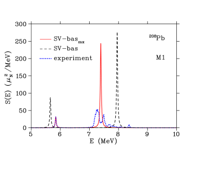
Figure 1: Strength functions of the M1 excitations in ²⁰⁸Pb calculated within RPA using the parametrization SV-bas Klüpfel et al. (2009) (black dashed line) and SV-bas${}_{{}_{\mbox{\scriptsize mx}}}$ as a modified variant thereof (red solid line) introduced in section IV. Experimental data taken from Refs. Köhler et al. (1987); Shizuma et al. (2008) are shown by the blue dotted line. The low-lying M1 state is at 5.84 MeV, hidden below the result from SV-bas${}_{{}_{\mbox{\scriptsize mx}}}$. The discrete peaks from RPA and the lower M1 mode have been broadened with a smearing parameter $\Delta=20$ keV to represent a smooth distribution.

The strength functions were obtained by folding the discrete RPA spectrum and the discrete experimental mode (lower M1 mode) with a Lorentzian of half-width $\Delta=20$ keV. The experimental data demonstrate the basic features of M1 strength in ²⁰⁸Pb: there is a very narrow peak at lower energy $E_{1}=5.84$ MeV and a broad resonance at $E_{2}=7.39$ MeV. The height of the lower peak is characterized by its integrated $B_{1}(M1)$ strength. Experimental mean energy and strength of the upper M1 resonance are computed from moments $m_{k}=\Sigma_{\nu}\,B_{\nu}(M1)\,E_{\nu}^{k}$ summed/integrated in the interval 6.6–8.1 MeV with the probabilities $B_{\nu}(M1)$ and the excitation energies $E_{\nu}$ taken from Refs. Köhler et al. (1987); Shizuma et al. (2008). We indicate this procedure by the notation $\sum B(M1)$ for that value. Note that we do not include in this interval the state with $E$ = 7.335 MeV (and possible $B(M1)$ = 1.8 $\mu^{2}_{N}$) from Ref. Shizuma et al. (2008) because of the uncertainty with the identification of its spin. We also note that the chosen smearing parameter $\Delta=20$ keV is sufficiently large to average out the fine structure of the experimental spectrum which is not essential for our analysis, but remains sufficiently small to resolve the spreading widths. The experimental strength distribution is composed from two data sets, below the neutron separation energy 7.37 MeV from Shizuma et al. (2008) and above from Köhler et al. (1987). It is thus not clear whether the dip between the peaks at 7.26 MeV and 7.47 MeV is a real effect. Inelastic proton scattering data Poltoratska et al. (2012); Birkhan et al. (2016) seems to indicate that the dip does not exist. Anyway, such detailed fragmentation structure cannot be described within RPA. Thus we use for comparison with RPA the average peak properties as explained above. Altogether, we have four observables $E_{1}$, $E_{2}$, $B_{1}(M1)$, and $\sum B(M1)$ which we use henceforth to characterize the M1 modes in ²⁰⁸Pb.

Fig. 1 shows theoretical results from two different parametrizations. The parametrization SV-bas${}_{{}_{\mbox{\scriptsize mx}}}$ (which is tuned to data such that theoretical and experimental curve for the lower peak at 5.84 MeV coincide) stands at the end of our investigations and will be discussed later. The results for SV-bas (computed here with the all spin-spin terms included, i.e. $\eta^{\vphantom{1}}_{\Delta s}=1$) are typical for most of the available Skyrme parametrizations. They agree qualitatively in that theory also produces two dominant peaks in the correct energy range. But the position of the peaks and their strengths differs too much from the data. Reasons for that and possible cures will be discussed in the following.

III.2 State of the art

It is well known that the properties of the low-energy M1 excitations in ²⁰⁸Pb in the RPA are mainly determined by two $ph$ configurations formed by the neutron’s ($\nu$) and proton’s ($\pi$) spin-orbit doublets $1i_{11/2}-1i_{13/2}$ and $1h_{9/2}-1h_{11/2}$. The main characteristics of these configurations are the $ph$ energy differences. Since the single-particle spectra produced by the various parametrizations of the Skyrme EDF are very different one can trace correlations between the values of these energy differences, parameters of the EDF, and the RPA results for the M1 excitations in ²⁰⁸Pb.

Let us introduce the notations

$$\varepsilon^{\nu}_{ph} = \varepsilon^{\nu}_{p}(1i^{\vphantom{*}}_{11/2})-\varepsilon^{\nu}_{h}(1i^{\vphantom{*}}_{13/2})\,,$$ (21)

$$\varepsilon^{\pi}_{ph} = \varepsilon^{\pi}_{p}(1h^{\vphantom{*}}_{9/2})-\varepsilon^{\pi}_{h}(1h^{\vphantom{*}}_{11/2})\,,$$ (22)

$$\bar{\varepsilon}^{\vphantom{1}}_{ph}=\frac{1}{2}\,\bigl{(}\,\varepsilon^{\nu}_{ph}+\varepsilon^{\pi}_{ph}\,\bigr{)}\,,\qquad\Delta\varepsilon^{\vphantom{1}}_{ph}=\varepsilon^{\nu}_{ph}-\varepsilon^{\pi}_{ph}\,.$$ (23)

The values of $\varepsilon^{\nu}_{ph}$ and $\varepsilon^{\pi}_{ph}$ along with the energies and the reduced probabilities of the excitation of the (isoscalar) $1^{+}_{1}$ state and the mean energies and the summed strengths of the (isovector) M1 resonance in ²⁰⁸Pb calculated within the self-consistent RPA for the parametrizations of the Skyrme EDF indicated in Sec. II.2 are presented in Figure 2. The effective M1 operator (15) with the renormalization constants $\xi_{s}$ and $\xi_{\,l}$ from Eq. (16) is used.

Figure 2: RPA results for energies $E_{n}$ and $B_{n}(M1)$ values of the two leading M1-modes in ²⁰⁸Pb for a variety of published Skyrme parametrizations as listed at the end of section II.2. For the energies, we show also the leading $1ph$ excitations $\varepsilon^{\pi}_{ph}$ or $\varepsilon^{\nu}_{ph}$, respectively. Experimental values are indicated by horizontal dotted lines. The parametrizations are grouped in those which omit tensor spin-orbit ($\eta^{\mbox{}}_{J}=0$, $C^{J}_{T}=0$) and those which use it ($\eta^{\mbox{}}_{J}=1$, $C^{J}_{T}\neq 0$). RPA results are considered for two options concerning the spin gradient terms $\propto s\Delta s$: $\eta^{\mbox{}}_{\Delta s}=1$ ($C_{T}^{\Delta s}\neq 0$) and $\eta^{\mbox{}}_{\Delta s}=0$ ($C_{T}^{\Delta s}=0$).

The shifts from mere $\varepsilon_{ph}$ to the corresponding RPA energies $E_{n}$ indicate the strength of residual interaction in the M1 channel. It is generally smaller than for the giant resonances. The figure reveals three main problems: First, some Skyrme-EDF parametrizations used with all spin terms [that means $\eta^{\mbox{}}_{\Delta s}=1$ in Eqs. (34) and is denoted by open circles and the label “with $\mbox{\boldmath$s$}\Delta\mbox{\boldmath$s$}$” in Fig. 2] lead to spin instability (imaginary RPA solutions) and thus have no entry in the plot (missing open circles). Second, the reduced probability $B_{1}(M1)$ of excitation of the first $1^{+}$ state significantly exceeds its experimental value for the most parametrizations, despite the quenching produced by the effective M1 operator. Third, the mismatch starts already at the level of pure $1ph$ energies $\varepsilon^{\nu}_{ph}$ which are definitely too large (upper panel) which can be tracked down to the fact that all parametrizations give too large values of $\Delta\varepsilon_{ph}$ as compared to the experiment (see Figure 3). As a result, none of the parametrizations listed in Figure 2 gives a satisfactory description of both M1-modes simultaneously. These problems were already found in earlier publications and the spin-orbit coupling was identified as one mechanism driving the M1 properties Nesterenko et al. (2010). We will now discuss that in more detail and explore ways for a solution.

III.3 Spin stability

Spin stability is a crucial issue in the construction of Skyrme parametrizations Stringari et al. (1976); Chabanat et al. (1998). The first is to check the stability of bulk matter which is done easily in terms of the LM parameters of the residual interaction. The LM parameters are related with the $C$-constants of the Skyrme-EDF by the following equations (see, e.g., Refs. Bender et al. (2002); Chamel et al. (2009))

$$F^{\vphantom{*}}_{0} = 2N_{0}\,[\,C^{\rho}_{0}+{\textstyle\frac{1}{2}}(\alpha+1)(\alpha+2)C^{\rho,\alpha}_{0}\rho^{\alpha}_{\mbox{\scriptsize eq}}+C^{\tau}_{0}k^{2}_{\mbox{\scriptsize F}}]\,,\qquad\;\;$$ (24a)

$$F^{\prime}_{0} = 2N_{0}\,[\,C^{\rho}_{1}+C^{\rho,\alpha}_{1}\rho^{\alpha}_{\mbox{\scriptsize eq}}+C^{\tau}_{1}k^{2}_{\mbox{\scriptsize F}}\,]\,,$$ (24b)

$$G^{\vphantom{*}}_{0} = 2N_{0}\,[\,C^{s}_{0}+C^{s,\alpha}_{0}\rho^{\alpha}_{\mbox{\scriptsize eq}}-C^{J}_{0}k^{2}_{\mbox{\scriptsize F}}\,]\,,$$ (24c)

$$G^{\prime}_{0} = 2N_{0}\,[\,C^{s}_{1}+C^{s,\alpha}_{1}\rho^{\alpha}_{\mbox{\scriptsize eq}}-C^{J}_{1}k^{2}_{\mbox{\scriptsize F}}\,]\,,$$ (24d)

$$F^{\vphantom{*}}_{1} = -2N_{0}C^{\tau}_{0}k^{2}_{\mbox{\scriptsize F}}\,,\;\,\quad F^{\prime}_{1}=-2N_{0}C^{\tau}_{1}k^{2}_{\mbox{\scriptsize F}}\,,$$ (24e)

$$G^{\vphantom{*}}_{1} = 2N_{0}C^{J}_{0}k^{2}_{\mbox{\scriptsize F}}\,,\qquad G^{\prime}_{1}=2N_{0}C^{J}_{1}k^{2}_{\mbox{\scriptsize F}}\,,$$ (24f)

where $N_{0}=2m^{*}k_{\mbox{\scriptsize F}}/(\pi\hbar)^{2}$, $k_{\mbox{\scriptsize F}}=(3\pi^{2}\rho_{\mbox{\scriptsize eq}}/2)^{1/3}$ is the Fermi momentum, and $\rho_{\mbox{\scriptsize eq}}$ is the equilibrium density of the infinite nuclear matter (INM). Eqs. (24) coincide with the definitions of Ref. Van Giai and Sagawa (1981) if the $C$-constants are expressed through the parameters of the Skyrme force by the standard formulas. However, Eqs. (24) produce $G_{L}$ and $G^{\prime}_{L}$ at variance with Ref. Van Giai and Sagawa (1981) for those parametrizations in which the $J^{2}$ terms are omitted ($\eta^{\vphantom{*}}_{J}=0$ and $C^{J}_{T}=0$) as noted in Lesinski et al. (2007). In particular, the parameters $G_{1}$ and $G^{\prime}_{1}$ are exactly equal to zero if the $J^{2}$ terms are absent in the Skyrme EDF. To ensure stability, the LM parameters should satisfy the following inequalities (see Migdal (1967))

$$\frac{F^{\vphantom{*}}_{L}}{2L+1}>-1\,,\qquad\frac{F^{\prime}_{L}}{2L+1}>-1\,,$$ (25a)

$$\frac{G^{\vphantom{*}}_{L}}{2L+1}>-1\,,\qquad\frac{G^{\prime}_{L}}{2L+1}>-1\,.$$ (25b)

Table 1: Landau-Migdal parameters of the Skyrme-EDFs listed in Figure 2.

EDF	$\eta^{\vphantom{*}}_{J}$	$x_{W}$	$F^{\vphantom{*}}_{0}$	$F^{\prime}_{0}$	$G^{\vphantom{*}}_{0}$	$G^{\prime}_{0}$	$F^{\vphantom{*}}_{1}$	$F^{\prime}_{1}$	$G^{\vphantom{*}}_{1}$	$G^{\prime}_{1}$	$N^{-1}_{0}$	$m^{*}/m$	$k_{\mbox{\scriptsize F}}$
											(MeV$\cdot$fm3)		(fm-1)
SIII	0	1	0.31	0.87	0.54	0.95	$-$0.71	0.49	0	0	207.8	0.76	1.29
SGII	0	1	$-$0.23	0.73	0.62	0.93	$-$0.64	0.52	0	0	196.1	0.79	1.33
SkM∗	0	1	$-$0.23	0.93	0.33	0.94	$-$0.63	0.62	0	0	194.6	0.79	1.33
RATP	0	1	$-$0.28	0.59	0.63	0.89	$-$1.00	0.56	0	0	230.2	0.67	1.33
T5	1	1	$-$0.10	1.96	$-$0.88	0.05	$-$0.00	$-$0.00	0.97	0.97	152.3	1.00	1.34
T6	1	1	0.06	1.43	$-$0.22	0.18	$-$0.00	$-$0.00	0.86	0.86	153.3	1.00	1.34
SkP	1	1	$-$0.10	1.42	$-$0.23	0.06	0.00	1.05	$-$0.18	0.97	152.7	1.00	1.34
SkI3	0	0	$-$0.32	0.65	1.90	0.85	$-$1.27	$-$0.84	0	0	267.2	0.58	1.33
SkI4	0	$\!\!\!\!-$0.99	$-$0.27	0.56	1.77	0.88	$-$1.05	$-$0.57	0	0	236.4	0.65	1.33
SkI5	0	1	$-$0.32	0.76	1.79	0.85	$-$1.26	$-$0.84	0	0	267.7	0.58	1.32
SLy4	0	1	$-$0.28	0.81	1.39	0.90	$-$0.92	$-$0.40	0	0	221.2	0.69	1.33
SLy5	1	1	$-$0.28	0.81	1.12	$-$0.14	$-$0.91	$-$0.39	0.25	1.04	220.1	0.70	1.33
SLy6	0	1	$-$0.28	0.80	1.41	0.90	$-$0.93	$-$0.41	0	0	223.0	0.69	1.33
SKX	0	0	0.24	1.56	$-$0.46	1.04	$-$0.02	0.98	0	0	156.1	0.99	1.32
SKXm	0	0	0.05	1.47	$-$0.29	1.02	$-$0.10	0.87	0	0	159.4	0.97	1.33
SKXce	0	0	0.24	1.52	$-$0.45	1.04	0.02	1.01	0	0	154.1	1.01	1.32
SkO	0	$\!\!\!\!-$1.13	$-$0.10	1.33	0.48	0.98	$-$0.31	0.16	0	0	171.2	0.90	1.33
SkO′	1	$\!\!\!\!-$0.58	$-$0.10	1.33	$-$1.61	0.79	$-$0.31	0.09	2.16	0.19	171.3	0.90	1.33
MSk1	1	1	0.07	1.47	$-$0.18	0.25	$-$0.00	$-$0.00	0.78	0.78	154.3	1.00	1.33
MSk3	1	1	0.07	1.30	$-$0.00	0.27	$-$0.00	$-$0.00	0.77	0.77	154.3	1.00	1.33
MSk9	1	1	0.07	1.30	$-$0.02	0.25	$-$0.00	$-$0.00	0.78	0.78	154.3	1.00	1.33
SV-bas	0	0.55	$-$0.05	1.20	0.00	0.99	$-$0.30	0.78	0	0	170.8	0.90	1.33
SV-K218	0	0.45	$-$0.12	1.18	0.02	0.99	$-$0.30	0.77	0	0	170.3	0.90	1.34
SV-kap00	0	1.33	$-$0.05	1.20	1.08	0.99	$-$0.30	$-$0.30	0	0	170.8	0.90	1.33
SV-mas07	0	1.02	$-$0.26	0.71	1.16	0.90	$-$0.90	$-$0.06	0	0	219.5	0.70	1.33
SV-sym34	0	0.29	$-$0.04	1.50	$-$0.29	0.99	$-$0.30	0.78	0	0	170.9	0.90	1.33
SV-min	0	0.83	$-$0.05	1.37	0.58	1.01	$-$0.14	0.07	0	0	160.9	0.95	1.34
SV-m56k6	0	0.79	$-$0.35	0.24	1.78	0.84	$-$1.33	$-$0.33	0	0	277.4	0.56	1.33
SV-m64k6	0	1.10	$-$0.30	0.40	1.30	0.87	$-$1.09	0.05	0	0	242.3	0.64	1.33
SAMi	1	0.31	$-$0.25	0.56	0.15	0.35	$-$0.97	0.05	1.03	0.54	228.0	0.68	1.33

Table 1 shows the LM parameters corresponding to the Skyrme-EDF parametrizations listed in Figure 2. The values of the spin-orbit parameter $x_{W}$ which will be discussed in Sec. III.4 are also given. The conditions (25) are fulfilled for all parameters from Table 1 except for the parameter $G^{\vphantom{*}}_{0}$ of SkO^′. However, as can be seen from Figure 2, the parametrizations T5, SkI4, SkO, SV-mas07, SV-sym34, SV-min, SV-m56k6, and SV-m64k6, for which the INM is stable, lead to the spin instability of the ground state of ²⁰⁸Pb in the case of $\eta^{\vphantom{1}}_{\Delta s}=1$, in spite of bulk stability as proven by Table 1. This instability appears only in certain finite nuclei and is generated by the spin surface terms $\propto{C}_{T}^{\Delta s}$, not contained in Eqs. (24) for the LM parameters (see also Ref. Pastore et al. (2015) where this question is discussed in more detail). On the other hand, Figure 2 shows that the inclusion of the terms proportional to $C_{T}^{\Delta s}$ into the Skyrme EDF usually decreases the energy of the $1^{+}_{1}$ state (compare open with filled circles). Exceptions from this general trend are SkP, SKX, and SKXce for which $E(1^{+}_{1})$ slightly increases if $\eta^{\vphantom{1}}_{\Delta s}=1$. If the downshift by the $C_{T}^{\Delta s}$ terms grows too large, it drives the finite nucleus to instability. All the Skyrme-EDF parametrizations shown in Figure 2 except for SkO^′ provide a stable ground state for ²⁰⁸Pb in case of $\eta^{\vphantom{1}}_{\Delta s}=0$ which is in agreement with the INM properties resulting from Table 1.

Note that the instability generated by the EDF SkO^′ disappears in the modified parametrization SkO${}^{\prime}_{\mbox{\scriptsize m}}$, in which the $C$-constants are determined by Eqs. (34) with $\eta^{\vphantom{1}}_{s}$ = $\eta^{\vphantom{1}}_{s,\alpha}$ = $\eta^{\vphantom{1}}_{\Delta s}$ = 0, $C^{\vphantom{*}}_{\mbox{\scriptsize N}}=300$ MeV$\cdot$fm³, $g=0.891$, and $g^{\prime}=1.39$. In this case we have $G^{\vphantom{*}}_{0}=-0.60$, $G^{\prime}_{0}$ = 2.24. The parameters $F^{\vphantom{*}}_{0,1}$, $F^{\prime}_{0,1}$, $G^{\vphantom{*}}_{1}$, and $G^{\prime}_{1}$ are not changed. Thus, the nuclear matter becomes stable. The parameters $g$ and $g^{\prime}$ in SkO${}^{\prime}_{\mbox{\scriptsize m}}$ have been adjusted to reproduce within the RPA the experimental energies of the M1 excitations in ²⁰⁸Pb, $E_{1}$ = 5.84 MeV and $E_{2}$ = 7.39 MeV. The $B(M1)$ values for the $1^{+}_{1}$ state and the isovector $M1$ resonance in ²⁰⁸Pb in this parametrization are equal to 1.9 $\mu^{2}_{N}$ and 16.9 $\mu^{2}_{N}$, respectively.

III.4 The impact of spin-orbit parameters

Figure 2 indicates that problems appear already at the level of the $1ph$ energies. This becomes even more apparent when looking at the average and difference $1ph$ energies (23) as shown in Figure 3. First, $\Delta\varepsilon_{ph}$ exceeds for most parametrizations the experimental value (0.29 MeV) by a factor of 3.4 (SAMi) to 7.5 (SkM^∗), except for SkI4, SkO, and SkO^′ for which the spin-orbit parameter is $x_{W}<0$ (see Table 1).

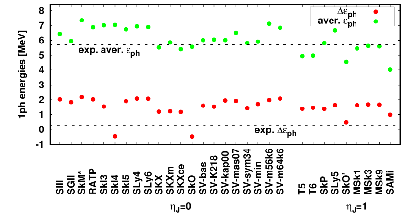
Figure 3: Average $1ph$ energy and difference as defined in Eq. (23) for the same selection of published Skyrme parametrizations as in Figure 2. Experimental values are indicated by horizontal dotted lines.

Second, for the parametrizations with $x_{W}>0$, the value of $B_{1}(M1)$ calculated with $\eta^{\vphantom{1}}_{\Delta s}=0$ is greater than its experimental value (2.0 $\mu^{2}_{N}$) by a factor of 2.2 (SkP) to 10 (SLy5). This together suggests that the values of $x_{W}$ and $\Delta\varepsilon_{ph}$ are key agents determining the RPA results for the M1 excitations in ²⁰⁸Pb.

To explore this further, we consider simultaneous variation of the spin-orbit parameters $x_{W}$ and $W_{0}$. To that end, we start from the set SV-bas Klüpfel et al. (2009), vary $x_{W}$, keeping all other model parameters frozen, and tune $W_{0}$ to reproduce the SHF binding energy of ²⁰⁸Pb at its experimental value 1636.43 MeV within the accuracy of 0.2 MeV. This is done for the option $\eta^{\vphantom{1}}_{\Delta s}=1$. Figure 4 shows the dependence of the RPA results for the first and second $1^{+}$ states in ²⁰⁸Pb on the parameter $x_{W}$ obtained in this way. The respective values of $\Delta\varepsilon_{ph}$, $\bar{\varepsilon}_{ph}$, and $W_{0}$ are also shown.

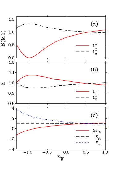
Figure 4: Dependence of the characteristics of M1 excitations in ²⁰⁸Pb on the parameter $x_{W}$ of the Skyrme EDF. Parametrization SV-bas Klüpfel et al. (2009) is used. (a) The reduced probabilities $B(M1)$ of the excitation of the first (solid red line) and second (dashed black line) $1^{+}$ states calculated in the RPA. (b) Same as in panel (a) but for the energies of these states. (c) The values of the energy differences $\Delta\varepsilon_{ph}$ (solid red line) and $\bar{\varepsilon}_{ph}$ (dashed black line), Eqs. (23), and the spin-orbit parameter $W_{0}$ (dotted blue line). All the quantities are given in units of their values obtained for the original parametrization Klüpfel et al. (2009). See text for more details.

All these quantities are given in units of their values obtained for the original set SV-bas Klüpfel et al. (2009) and shown in Figures 2 and 3 [$B_{1}(M1)$ = 5.5 $\mu^{2}_{N}$, $B_{2}(M1)$ = 17.4 $\mu^{2}_{N}$, $E_{1}$ = 5.66 MeV, $E_{2}$ = 7.95 MeV, $\Delta\varepsilon_{ph}$ = 1.60 MeV, $\bar{\varepsilon}_{ph}$ = 6.02 MeV] and the value $W_{0}$ = 124.634 MeV$\cdot$fm⁵. The $B_{1}(M1)$ shows the strongest dependence on $x_{W}$. In fact, one can obtain any value of $B_{1}(M1)<$ 6 $\mu^{2}_{N}$ by decreasing the parameter $x_{W}$. The experimental value $B_{1}(M1)$ = 2 $\mu^{2}_{N}$ is obtained at $x_{W}<$ 0. The values of $E_{1}$, $E_{2}$, and $B_{2}(M1)$ depend on $x_{W}$ to much lesser extent. The energy difference $\Delta\varepsilon_{ph}$ also shows a strong dependence on $x_{W}$, while the value of $\bar{\varepsilon}_{ph}$ is nearly constant (it is changed within 2.2% in the considered interval of $x_{W}$). The trend of $\Delta\varepsilon_{ph}$ with $x_{W}$ is monotonous. This allows to transform the dependencies shown in panels (a) and (b) of Fig. 4 into analogous dependencies on $\Delta\varepsilon_{ph}$.

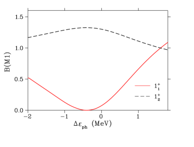
Figure 5: Same as in Fig. 4 but for the dependence of the reduced probabilities $B(M1)$ on the value of the energy difference $\Delta\varepsilon_{ph}$.

The results are shown in Fig. 5, where again we see the crucial dependence of $B_{1}(M1)$ on $\Delta\varepsilon_{ph}$ at the constant $\bar{\varepsilon}_{ph}$. This dependence explains why the parametrization SkO${}^{\prime}_{\mbox{\scriptsize m}}$ introduced in Sec. III.3 gives nice agreement with the experimental value of $B_{1}(M1)$: it has negative $x_{W}=-0.58$ and thus a value of $\Delta\varepsilon_{ph}$ = 0.48 MeV which is closest to the experimental value 0.29 MeV. The other Skyrme-EDF parametrizations have generally too large $\Delta\varepsilon_{ph}$ which leads to significant overestimation of the $B_{1}(M1)$. The impact of the value of $\Delta\varepsilon_{ph}$ on the properties of M1 excitations in ²⁰⁸Pb was pointed out in Vesely et al. (2009); Nesterenko et al. (2010).

IV Toward better reproduction of M1 modes

The results presented in Sec. III.4 show that spin-orbit parameters are most decisive for the M1-modes. And, of course, the parameters of the spin-spin terms play an equally important role. This motivates us to check the chances to find a Skyrme functional in standard form which provides a good description of M1-modes together with traditionally good modeling of ground state properties. At present stage, it is too early to launch a fully fledged least-squares fitting scheme Klüpfel et al. (2009); Kortelainen et al. (2010); Dobaczewski et al. (2014) particularly because a high precision RPA computation of M1-modes is far too expensive. Thus, for a first exploration, we employ a simple-minded, restricted fitting procedure: We start from a given Skyrme parametrization, keep all model parameters at their given value except for the spin-orbit parameters $C_{T}^{\nabla J}$ (alias $x_{W}$, $W_{0}$) and the spin-spin parameters $\,C_{T}^{s}$, $\,C_{T}^{s,\alpha}$, and $\,C_{T}^{\Delta s}$. The spin-spin parameters play no role for ground states of even-even nuclei. Thus we exploit here the freedom of not yet fixed parameters. However, the spin-orbit parameters enter ground state properties. Here we have to check that re-tuning does not destroy ground-state quality.

To keep the number of free spin-spin parameters low, we set $\eta^{\vphantom{1}}_{s,\alpha}$ = $\eta^{\vphantom{1}}_{\Delta s}$ = 0 and determine $\,C_{T}^{s}$ by Eqs. (34) with $\eta^{\vphantom{1}}_{s}$ = 0 and the fitting parameters $g$ and $g^{\prime}$ at $C^{\vphantom{*}}_{\mbox{\scriptsize N}}=300$ MeV$\cdot$fm³. After all, we have four free parameters $x_{W}$, $W_{0}$, $g$, and $g^{\prime}$ which are determined by adjusting four observables in ²⁰⁸Pb: the binding energy and the RPA results for the M1 energies $E_{1}$ and $E_{2}$ and the transition probability $B_{1}(M1)$ to their experimental values. Note that here we use, as before, the effective M1 operator (15) with the renormalization constants $\xi_{s}$ and $\xi_{\,l}$ from Eq. (16). This fitting procedure is applied to a subset of the parametrizations shown in Figure 2. The modified parametrizations thus obtained are marked by an index “m”.

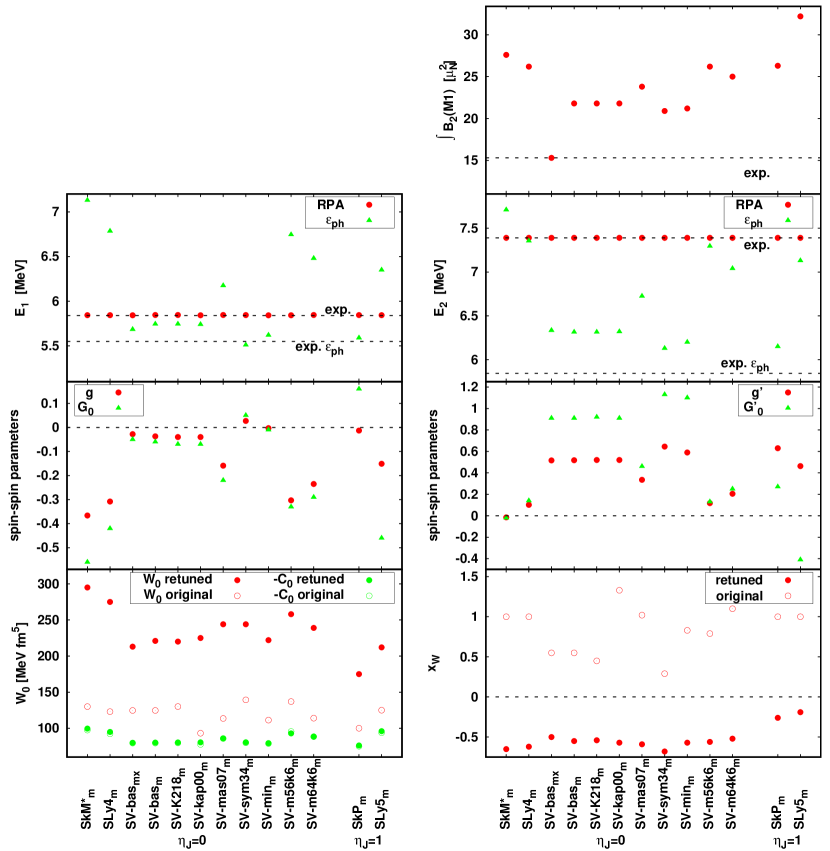
Figure 6: Results for the re-tuned parametrizations. Lower two panels: spin-orbit parameters $x_{W}$, $W_{0}$ (filled circles), and $-C_{0}^{\nabla J}$ (abbreviated $-C_{0}$ in the legend) together with their original values (open circles); spin-spin LM parameters $G_{0}$ and $G^{\prime}_{0}$ together with the interaction parameters $g$ and $g^{\prime}$ defined in Eqs. (34). Upper two panels: the M1 energies $E_{1}$ and $E_{2}$ together with their corresponding $1ph$ energies $\varepsilon^{\pi}_{ph}$ and $\varepsilon^{\nu}_{ph}$ and the $B(M1)$ strength for the upper M1 mode integrated over the interval 6.6–8.1 MeV. Experimental values are indicated by horizontal faint dashed lines.

Resulting re-tuned model parameters and properties of M1-modes are shown in Figure 6 and the corresponding re-tuned spin-orbit and spin-spin parameters are given in quantitative detail in Table 2.

Table 2: Parameters $\eta_{J}$, $x_{W}$, $W_{0}$, $g$, and $g^{\prime}$ of the modified Skyrme EDFs. Parameters $g$ and $g^{\prime}$ of the Landau-Migdal interaction (13) are taken from Ref. Migli et al. (1991).

EDF	$\eta^{\vphantom{*}}_{J}$	$x_{W}$	$W_{0}$	$g$	$g^{\prime}$
			(MeV$\cdot$fm5)
SkM${}^{*}_{{}_{\mbox{\scriptsize m}}}$	0	$-$0.65	295	$-$0.366	$-$0.015
SLy4${}_{{}_{\mbox{\scriptsize m}}}$	0	$-$0.62	275	$-$0.308	0.102
SV-bas${}_{{}_{\mbox{\scriptsize mx}}}$	0	$-$0.50	213	$-$0.028	0.516
SV-bas${}_{{}_{\mbox{\scriptsize m}}}$	0	$-$0.55	221	$-$0.037	0.518
SV-K218${}_{{}_{\mbox{\scriptsize m}}}$	0	$-$0.54	220	$-$0.040	0.520
SV-kap00${}_{{}_{\mbox{\scriptsize m}}}$	0	$-$0.57	225	$-$0.040	0.520
SV-mas07${}_{{}_{\mbox{\scriptsize m}}}$	0	$-$0.59	244	$-$0.159	0.335
SV-sym34${}_{{}_{\mbox{\scriptsize m}}}$	0	$-$0.68	244	0.027	0.645
SV-min${}_{{}_{\mbox{\scriptsize m}}}$	0	$-$0.57	222	$-$0.003	0.590
SV-m56k6${}_{{}_{\mbox{\scriptsize m}}}$	0	$-$0.56	258	$-$0.303	0.118
SV-m64k6${}_{{}_{\mbox{\scriptsize m}}}$	0	$-$0.52	239	$-$0.235	0.205
SkP${}_{{}_{\mbox{\scriptsize m}}}$	1	$-$0.26	175	$-$0.013	0.630
SLy5${}_{{}_{\mbox{\scriptsize m}}}$	1	$-$0.19	212	$-$0.151	0.463
Landau-Migdal				0.1	0.75

As expected from the exploration in section III.4, all re-tuned $x_{W}$ parameters are negative, most of them in the interval between $-0.6$ and $-0.5$. Exceptions are SkP${}_{{}_{\mbox{\scriptsize m}}}$ and SLy5${}_{{}_{\mbox{\scriptsize m}}}$ which have higher $x_{W}$ due to the $J^{2}$ terms in these parametrizations which contribute also to the single-particle spin-orbit potential. The re-tuned parameters $W_{0}$ are all rather large. This seemingly happens to compensate the negative $x_{W}$. The left lower panel of Figure 6 shows also the isoscalar spin-orbit parameter $C_{0}^{\nabla J}=-{\textstyle\frac{1}{4}}(2+x_{W})W_{0}$. This combination shows much less variations over the different forces and, in particular, remains practically unmodified by re-tuning. It is the isovector spin-orbit term proportional to $C_{1}^{\nabla J}=-{\textstyle\frac{1}{4}}x_{W}W_{0}$ which makes the difference. Seeing the dramatic differences in spin-orbit parameters, one wonders what happens to the overall quality of the parametrization. This question will be addressed farther below.

The spin-spin coupling parameters $g$ and $g^{\prime}$ show some correlation with the effective mass $m^{*}/m$ of a parametrization. The sets SkP${}_{{}_{\mbox{\scriptsize m}}}$, SV-bas${}_{{}_{\mbox{\scriptsize m}}}$, SV-K218${}_{{}_{\mbox{\scriptsize m}}}$, SV-kap00${}_{{}_{\mbox{\scriptsize m}}}$, SV-sym34${}_{{}_{\mbox{\scriptsize m}}}$, and SV-min${}_{{}_{\mbox{\scriptsize m}}}$ all having $m^{*}/m\approx 1$ have similar values which are also close to the values $g=0.1$, $g^{\prime}=0.75$ used previously in the non-self-consistent TFFS (see Migli et al. (1991)) while the other parametrizations having lower $m^{*}/m$ also produce lower $g$ and $g^{\prime}$.

The LM parameters $G^{\vphantom{*}}_{0}$ and $G^{\prime}_{0}$ in Figure 6 stay all safely above $-1$ and thus lead to stable INM which also persists in finite nuclei because the modified parametrizations set the critical gradient spin term to zero.

The RPA energies $E_{n}$ stay by construction at the experimental values. We show them (second panels from above) to illustrate the span toward the pure $1ph$ energies $\varepsilon^{\pi}_{ph}$ (left) and $\varepsilon^{\nu}_{ph}$ (right). Let us concentrate first on the isoscalar mode (left). The up-shift by the residual interaction is small for the parametrizations with $m^{*}/m\approx 1$, in accordance with the small values of $g$ or $G^{\vphantom{*}}_{0}$. In these cases, the $1ph$ energies represent already a good estimate of $E_{1}$ and the theoretical $\varepsilon^{\pi}_{ph}$ lie close to the experimental value (faint dotted line). Lower effective masses increase $\varepsilon^{\pi}_{ph}$, away from the wanted $E_{1}$, and need more residual interaction to compensate. The impact of residual interaction is much larger for the isovector modes (right), again in accordance with the much larger spin coupling parameter $g^{\prime}$. In that case, we also have the problem that all theoretical $\varepsilon^{\nu}_{ph}$ are much higher than the experimental value of 5.84 MeV.

The upper right panel of Figure 6 shows the $B(M1)$ strength integrated over the vicinity of the upper M1-mode. One observes a close relation between $g^{\prime}$ and the isovector $B(M1)$ value: An increase of $g^{\prime}$ reduces the $B(M1)$ value. This is due to the increase of the ground state correlations ($Y$-components of the RPA transition amplitudes) which decreases the transition probabilities in the magnetic case in contrast to the electric case where the ground state correlations add coherently. The parametrizations SkP${}_{{}_{\mbox{\scriptsize m}}}$ and SLy5${}_{{}_{\mbox{\scriptsize m}}}$ behave slightly different because as mentioned before in these parametrizations the $J^{2}$ terms are included. These terms have a noticeable impact on the $B(M1)$ values that can be estimated with the help of the single-particle part of the RPA energy-weighted sum rule (EWSR) $m^{\mbox{\scriptsize s.p.}}_{1}$. In the case of the M1 excitations with the operator (15) it has the form

$$m^{\mbox{\scriptsize s.p.}}_{1}=\frac{1}{2}\,\mbox{Tr}\,\bigl{(}\rho\,\bigl{[}\bigl{[}\,\mbox{\boldmath$Q$},\,h\,\bigr{]},\cdot\,\mbox{\boldmath$Q$}\,\bigr{]}\bigr{)}$$ (26)

(see Ref. Tselyaev et al. (2011) for more details). In our self-consistent RPA calculations we obtain that this EWSR is fulfilled within 0.2% in the case of the Skyrme-EDF parametrizations without the $J^{2}$ terms ($\eta^{\vphantom{*}}_{J}=0$). In the case of the SkP${}_{{}_{\mbox{\scriptsize m}}}$ and SLy5${}_{{}_{\mbox{\scriptsize m}}}$ parametrizations ($\eta^{\vphantom{*}}_{J}=1$), this EWSR is exceeded by 19 and 25%, respectively.

Generally, we see in the upper right panel of Figure 6 that the theoretical isovector $B(M1)$ strengths, even for the best parameter sets, are significantly larger than the experimental values. Here one has to bear in mind that the experimental data in Figure 6 have been integrated only up to 8.1 MeV. We know from previous beyond-RPA calculations within the Landau-Migdal approach Kamerdzhiev et al. (1993) that the theoretical strength is distributed by coupling to $2ph$ states up to much higher energies. Such spectral fragmentation is also seen in data. A recent $(p,p^{\prime})$ experiment Poltoratska et al. (2012); Birkhan et al. (2016) reports a summed $B(M1)$ = 20.5(1.3) $\mu^{2}_{N}$ when integrated up to 9 MeV, a value which would fit nicely into the theoretical results of Figure 6. This situation reminds us at the case of the Gamow-Teller resonance in ²⁰⁸Pb where only half of the sum-rule strength was concentrated in one single strong resonance and the rest was missing. Calculations within a $2ph$ model Drożdż et al. (1990) (where one of the authors was involved) predicted a long tail which included the other half of the total strength. Ten years later the predicted strength had been detected experimentally. Thus, excess of the strength can be corrected in extended RPA models including particle-phonon coupling that give also rise to a shift of the RPA strength to higher energies.

So far, we have computed the $B(M1)$ strengths with the effective M1 operator using the renormalization constants $\xi_{s}$ and $\xi_{\,l}$ as defined in Eq. (16). This construction is designed to account for correlation effects not included in the actual Hilbert space. Thus the $\xi_{s}$ and $\xi_{\,l}$ can, in principle, be different for the different models. This was exploited in the variant SV-bas${}_{{}_{\mbox{\scriptsize mx}}}$ where $\xi_{s}$ was used tentatively as further free parameter and the isovector $B(M1)$ strength as additional data point. The fitted renormalization constants for SV-bas${}_{{}_{\mbox{\scriptsize mx}}}$ are $\xi_{s}=0.154$ while $\xi_{\,l}=0$ is chosen in accordance with the condition (20). The results in Figure 6 shows that this strategy allows to produce better $B(M1)$ strength while maintaining the quality of the other observables. Note that the changes in $\xi_{s}$ and $\xi_{\,l}$ are, in fact, small which rather supports the original choices (16). Anyway, this fit of renormalization constants should be considered as an exploration of still loose ends in modeling. Playing with these values needs yet to be supported by sound many-body theory.

As argued above, spin-orbit parameters have not only huge impact on M1 modes, but also on ground state properties. Thus a dramatic change of isovector spin-orbit coupling as implied in the re-tuned parametrizations could have unwanted side effects on the quality concerning the reproduction of ground state properties.

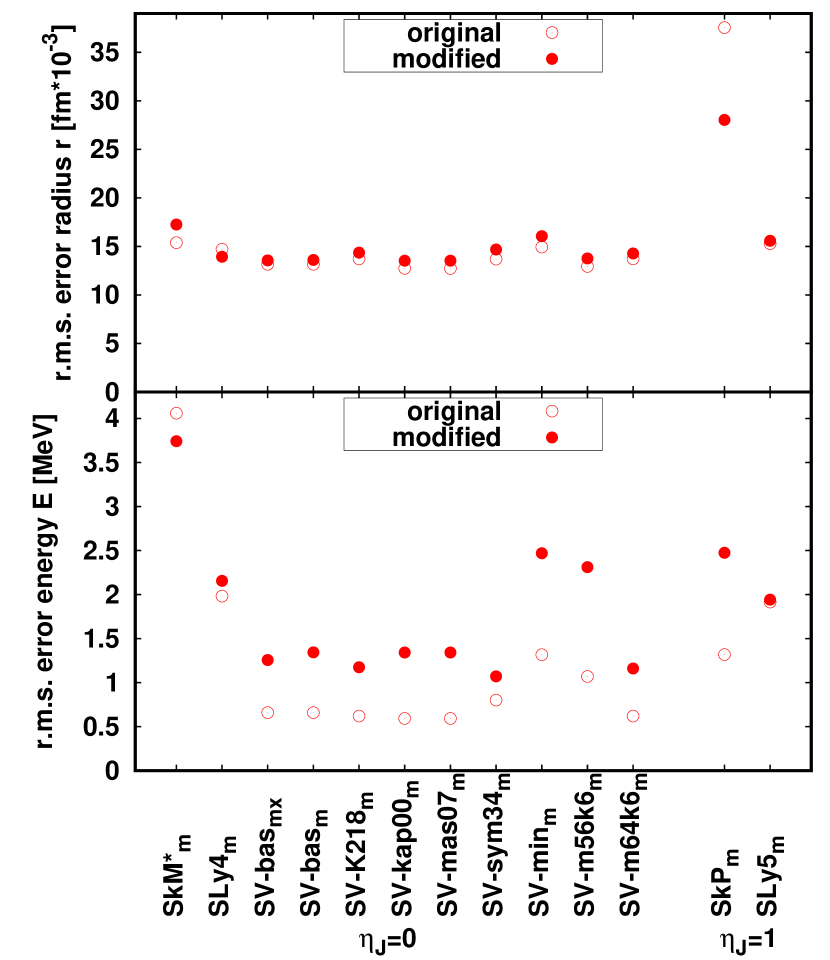
Figure 7: Average quality of the re-tuned parametrizations quantified in terms of root-mean-square deviation of energy and charge radii taken over the set of spherical nuclei from Klüpfel et al. (2009).

Figure 7 shows the performance of the refitted parametrizations with respect to ground state energy and charge radius. The change of spin-orbit parameters leaves the overall quality basically conserved. There is no effect at all for the radii. Energy reacts more sensitively which is little surprise because pairing in semi-magic nuclei is highly sensitive to level density which, of course, is influenced by spin-orbit splitting. Note that particularly the more recent, well fitted parametrizations show a loss of energy quality, fortunately in acceptable bounds. Still, the simple minded re-tuning strategy spoils somewhat the overall quality of the parametrizations, the better the quality originally the larger the loss. Moreover, there are more subtle observables as pairing gaps and isotopic shifts of radii. The latter are known to be sensitive to the isovector spin-orbit term Reinhard and Flocard (1995), for pairing gaps it is likely. All this calls for more continued investigations, more systematic fits, and correlation analysis Dobaczewski et al. (2014) to clearly work out the impact of information from M1 modes on nuclear density functionals.

So far, we have discussed the properties of M1 modes in terms of two energies and $B(M1)$ values. Let us finally look again at the whole spectral distribution as it was shown in Fig. 1. The results obtained with the freshly re-tuned parametrization SV-bas${}_{{}_{\mbox{\scriptsize mx}}}$ agree, by construction, nicely with experimental data. Comparison with the original SV-bas shows the gain. Similar plots would be obtained when comparing original and re-tuned versions of the other parametrizations. But Fig. 1 also points toward the yet open problems with the upper M1 mode: First, the strength is overestimated, and second, its spectral fragmentation is not described at all. Both problems are related to each other as discussed above. The hope is that a beyond-RPA modeling within the phonon-coupling model could deliver the missing pieces.

V Conclusions

In the present paper, we investigate the dependence of the spin-dependent part of the $ph$-interaction on the parameters of Skyrme energy density functional (EDF). This part is relevant for computing magnetic excitation modes within the self-consistent random-phase approximation (RPA). We considered here, in particular, magnetic dipole (M1) modes in ²⁰⁸Pb as test case. The M1 modes are found depend crucially on the spin-orbit term and on the spin-spin interaction. The latter has no influence on ground state properties and generally only weak relations to natural-parity modes in even nuclei and is thus open to adjustment. The spin-orbit term is to some extend constrained by ground-state properties. However, we find that ground states leave enough leeway in them to accommodate the properties of M1 modes with only small sacrifices on the overall quality of the ground state properties. We have tested that on a variety of 12 published Skyrme EDFs.

In the analysis, we guide by the Landau-Migdal (LM) parameters from the Theory of Finite Fermion Systems (TFFS) which are weak in the isoscalar spin part and strongly repulsive in the isovector part. The re-tuned Skyrme EDFs deliver LM parameters in accordance with the TFFS. The relations between the LM parameters and the parameters of the Skyrme-EDF serve also for a quick first check of spin stability of the chosen parameter set.

As open questions remain the fragmentation and the magnitude of the isovector M1 resonance. Both are connected with more complex configurations beyond RPA, e.g., the coupling to the low-lying phonons (strong modes in each angular momentum channel). This, however, requires that all relevant phonons, also in the magnetic channels, are correctly described by RPA. The present survey is a first step toward a proper description of magnetic excitations in the framework of Skyrme-EDF and so paves the way to subsequent beyond-RPA calculations.

Appendix A Local densities and currents

Let us introduce the isoscalar ($T=0$) and isovector ($T=1$) single-particle density matrices

$$\rho^{\vphantom{*}}_{T}(\mbox{\boldmath$r$},\sigma;\mbox{\boldmath$r$}^{\prime},\sigma^{\prime}) = \rho^{\vphantom{*}}_{n}(\mbox{\boldmath$r$},\sigma;\mbox{\boldmath$r$}^{\prime},\sigma^{\prime})$$ (27)

$$+ (-1)^{T}\rho^{\vphantom{*}}_{p}(\mbox{\boldmath$r$},\sigma;\mbox{\boldmath$r$}^{\prime},\sigma^{\prime})\,,$$

where $\rho^{\vphantom{*}}_{n}(\mbox{\boldmath$r$},\sigma;\mbox{\boldmath$r$}^{\prime},\sigma^{\prime})$ and $\rho^{\vphantom{*}}_{p}(\mbox{\boldmath$r$},\sigma;\mbox{\boldmath$r$}^{\prime},\sigma^{\prime})$ are the neutron’s and proton’s density matrices. The expressions for the local densities and currents entering Eq. (12) in terms of these matrices read

$$\rho^{\vphantom{*}}_{T}(\mbox{\boldmath$r$}) = \sum_{\sigma}\rho^{\vphantom{*}}_{T}(\mbox{\boldmath$r$},\sigma;\mbox{\boldmath$r$},\sigma)\,,$$ (28)

$$\tau^{\vphantom{*}}_{T}(\mbox{\boldmath$r$}) = \sum_{\sigma}\nabla\cdot\nabla^{\prime}\,\rho^{\vphantom{*}}_{T}\bigl{.}(\mbox{\boldmath$r$},\sigma;\mbox{\boldmath$r$}^{\prime},\sigma)\bigr{|}_{\mbox{\scriptsize\boldmath$r$}=\mbox{\scriptsize\boldmath$r^{\prime}$}}\,,$$ (29)

$$\mbox{\boldmath$J$}^{\vphantom{*}}_{T}(\mbox{\boldmath$r$}) = i\sum_{\sigma,\,\sigma^{\prime}}\,\bigl{[}(\mbox{\boldmath$\sigma$})_{\sigma^{\prime},\,\sigma}\times\nabla\bigr{]}\,\rho^{\vphantom{*}}_{T}\bigl{.}(\mbox{\boldmath$r$},\sigma;\mbox{\boldmath$r$}^{\prime},\sigma^{\prime})\bigr{|}_{\mbox{\scriptsize\boldmath$r$}=\mbox{\scriptsize\boldmath$r^{\prime}$}}\qquad$$ (30)

for the time-even quantities and

$$\mbox{\boldmath$s$}^{\vphantom{*}}_{T}(\mbox{\boldmath$r$}) = \sum_{\sigma,\,\sigma^{\prime}}\,(\mbox{\boldmath$\sigma$})_{\sigma^{\prime},\,\sigma}\;\rho^{\vphantom{*}}_{T}(\mbox{\boldmath$r$},\sigma;\mbox{\boldmath$r$},\sigma^{\prime})\,,$$ (31)

$$\mbox{\boldmath$T$}^{\vphantom{*}}_{T}(\mbox{\boldmath$r$}) = \sum_{\sigma,\,\sigma^{\prime}}\,(\mbox{\boldmath$\sigma$})_{\sigma^{\prime},\,\sigma}\,\nabla\cdot\nabla^{\prime}\,\rho^{\vphantom{*}}_{T}\bigl{.}(\mbox{\boldmath$r$},\sigma;\mbox{\boldmath$r$}^{\prime},\sigma^{\prime})\bigr{|}_{\mbox{\scriptsize\boldmath$r$}=\mbox{\scriptsize\boldmath$r^{\prime}$}}\,,\qquad$$ (32)

$$\mbox{\boldmath$j$}^{\vphantom{*}}_{T}(\mbox{\boldmath$r$}) = \frac{i}{2}\sum_{\sigma}\,\bigl{(}\nabla^{\prime}-\nabla\bigr{)}\,\rho^{\vphantom{*}}_{T}\bigl{.}(\mbox{\boldmath$r$},\sigma;\mbox{\boldmath$r$}^{\prime},\sigma)\bigr{|}_{\mbox{\scriptsize\boldmath$r$}=\mbox{\scriptsize\boldmath$r^{\prime}$}}$$ (33)

for the time-odd quantities.

For the local densities $\tau_{p}(\mbox{\boldmath$r$})$, $\tau_{n}(\mbox{\boldmath$r$})$, and $\rho_{p}(\mbox{\boldmath$r$})$ in Eqs. (9) and (11) we have $\tau_{p}=(\tau^{\vphantom{*}}_{0}-\tau^{\vphantom{*}}_{1})/2$, $\tau_{n}=(\tau^{\vphantom{*}}_{0}+\tau^{\vphantom{*}}_{1})/2$, $\rho_{p}=(\rho^{\vphantom{*}}_{0}-\rho^{\vphantom{*}}_{1})/2$.

Appendix B Parameters of the Skyrme EDF

The following equations establish the relation between the $C$-constants in Eq. (12) and the parameters of the Skyrme force $t_{0}$, $x_{0}$, $t_{1}$, $x_{1}$, $t_{2}$, $x_{2}$, $t_{3}$, $x_{3}$, $W_{0}$, and $x_{W}$

$$\begin{array}[]{llllll}C_{0}^{\rho}&=&{\textstyle\frac{3}{8}}t_{0}\,,&C_{1}^{\rho}&=&-{\textstyle\frac{1}{4}}t_{0}({\textstyle\frac{1}{2}}+x_{0})\,,\\ C_{0}^{\rho,\alpha}&=&{\textstyle\frac{1}{16}}t_{3}\,,&C_{1}^{\rho,\alpha}&=&-{\textstyle\frac{1}{24}}t_{3}({\textstyle\frac{1}{2}}+x_{3})\,,\\ C_{0}^{\Delta\rho}&=&-{\textstyle\frac{9}{64}}t_{1}+{\textstyle\frac{5}{64}}t_{2}+{\textstyle\frac{1}{16}}t_{2}x_{2}\,,&C_{1}^{\Delta\rho}&=&{\textstyle\frac{1}{32}}\big{[}3t_{1}({\textstyle\frac{1}{2}}+x_{1})+t_{2}({\textstyle\frac{1}{2}}+x_{2})\big{]}\,,\\ C_{0}^{\tau}&=&{\textstyle\frac{3}{16}}t_{1}+{\textstyle\frac{5}{16}}t_{2}+{\textstyle\frac{1}{4}}t_{2}x_{2}\,,&C_{1}^{\tau}&=&-{\textstyle\frac{1}{8}}\big{[}t_{1}({\textstyle\frac{1}{2}}+x_{1})-t_{2}({\textstyle\frac{1}{2}}+x_{2})\big{]}\,,\\ C_{0}^{J}&=&{\textstyle\frac{1}{8}}\big{[}t_{1}\big{(}{\textstyle\frac{1}{2}}-x_{1}\big{)}-t_{2}\big{(}{\textstyle\frac{1}{2}}+x_{2}\big{)}\big{]}\eta^{\vphantom{1}}_{J}\,,&C_{1}^{J}&=&{\textstyle\frac{1}{16}}(t_{1}-t_{2})\,\eta^{\vphantom{1}}_{J}\,,\\ C_{0}^{\nabla J}&=&-{\textstyle\frac{1}{4}}(2+x_{W})W_{0}\,,&C_{1}^{\nabla J}&=&-{\textstyle\frac{1}{4}}x_{W}W_{0}\,,\\ C_{0}^{s}&=&{\textstyle\frac{1}{2}}C^{\vphantom{*}}_{\mbox{\scriptsize N}}\,g-{\textstyle\frac{1}{4}}t_{0}\big{(}{\textstyle\frac{1}{2}}-x_{0}\big{)}\eta^{\vphantom{1}}_{s}\,,&C_{1}^{s}&=&{\textstyle\frac{1}{2}}C^{\vphantom{*}}_{\mbox{\scriptsize N}}\,g^{\prime}-{\textstyle\frac{1}{8}}t_{0}\,\eta^{\vphantom{1}}_{s}\,,\\ C_{0}^{s,\alpha}&=&-{\textstyle\frac{1}{24}}t_{3}({\textstyle\frac{1}{2}}-x_{3})\,\eta^{\vphantom{1}}_{s,\alpha}\,,&C_{1}^{s,\alpha}&=&-{\textstyle\frac{1}{48}}t_{3}\,\eta^{\vphantom{1}}_{s,\alpha}\,,\\ C_{0}^{\Delta s}&=&{\textstyle\frac{1}{32}}\big{[}3t_{1}\big{(}{\textstyle\frac{1}{2}}-x_{1}\big{)}+t_{2}\big{(}{\textstyle\frac{1}{2}}+x_{2}\big{)}\big{]}\eta^{\vphantom{1}}_{\Delta s}\,,&C_{1}^{\Delta s}&=&{\textstyle\frac{1}{64}}(3t_{1}+t_{2})\,\eta^{\vphantom{1}}_{\Delta s}\,.\end{array}$$ (34)

The formulas for the spin-orbit constants $C_{T}^{\nabla J}$ imply the parametrization introduced in Reinhard and Flocard (1995); Sharma et al. (1995) in which the spin-orbit term of the interaction is treated in the Hartree approximation. The parameters $W_{0}$ and $x_{W}$ are related with the constants $b^{\vphantom{*}}_{4}$ and $b^{\prime}_{4}$ of Ref. Reinhard and Flocard (1995) by the formulas: $W_{0}=2b_{4}$, $x_{W}=b^{\prime}_{4}/b^{\vphantom{*}}_{4}$. The parameter $\eta^{\vphantom{1}}_{J}=1$ if the $J^{2}$ terms are included in the Skyrme EDF and $\eta^{\vphantom{1}}_{J}=0$ if not. In the standard parametrizations, the parameters $x_{W}$, $\eta^{\vphantom{1}}_{s}$, $\eta^{\vphantom{1}}_{s,\alpha}$, and $\eta^{\vphantom{1}}_{\Delta s}$ are equal to 1, the parameters $g$ and $g^{\prime}$ are equal to 0.

References

- Bender et al. (2003) M. Bender, P.-H. Heenen, and P.-G. Reinhard, Rev. Mod. Phys. 75, 121 (2003).
- Migdal (1967) A. B. Migdal, Theory of Finite Fermi Systems and Application to Atomic Nuclei (Wiley, New York, 1967).
- Ring and Speth (1973) P. Ring and J. Speth, Phys. Lett. B 44, 477 (1973).
- Borzov et al. (1984) I. N. Borzov, S. V. Tolokonnikov, and S. A. Fayans, Sov. J. Nucl. Phys. 40, 732 (1984).
- Speth and Wambach (1991) J. Speth and J. Wambach, in Electric and Magnetic Giant Resonances in Nuclei, Vol. International Review of Nuclear Physics, Vol. 7, edited by J. Speth (World Scientific, 1991) pp. 2–87.
- Vautherin and Brink (1972) D. Vautherin and D. Brink, Phys. Rev. C 5, 626 (1972).
- Beiner et al. (1975) M. Beiner, H. Flocard, N. Van Giai, and P. Quentin, Nucl. Phys. A 238, 29 (1975).
- Bartel et al. (1982) J. Bartel, P. Quentin, M. Brack, C. Guet, and H.-B. Håkansson, Nucl. Phys. A 386, 79 (1982).
- Brack et al. (1985) M. Brack, C. Guet, and H.-B. Håkansson, Phys. Rep. 123, 275 (1985).
- Klüpfel et al. (2009) P. Klüpfel, P.-G. Reinhard, T. J. Bürvenich, and J. A. Maruhn, Phys. Rev. C 79, 034310 (2009).
- Speth et al. (2014) J. Speth, S. Krewald, F. Grümmer, P. G. Reinhard, N. Lyutorovich, and V. Tselyaev, Nucl. Phys. A928, 17 (2014).
- Wienhard et al. (1982) K. Wienhard, K. Ackermann, K. Bangert, U. E. P. Berg, C. Bläsing, W. Naatz, A. Ruckelshausen, D. Rück, R. K. M. Schneider, and R. Stock, Phys. Rev. Lett. 49, 18 (1982).
- Köhler et al. (1987) R. Köhler, J. A. Wartena, H. Weigmann, L. Mewissen, F. Poortmans, J. P. Theobald, and S. Raman, Phys. Rev. C 35, 1646 (1987).
- Laszewski et al. (1988) R. M. Laszewski, R. Alarcon, D. S. Dale, and S. D. Hoblit, Phys. Rev. Lett. 61, 1710 (1988).
- Shizuma et al. (2008) T. Shizuma, T. Hayakawa, H. Ohgaki, T. Toyokawa, T. Komatsubara, N. Kikuzawa, A. Tamii, and H. Nakada, Phys. Rev. C 78, 061303(R) (2008).
- Bertsch (1981) G. F. Bertsch, Nuclear Physics A 354, 157c (1981).
- Vergados (1971) J. D. Vergados, Phys. Lett. B 36, 12 (1971).
- Speth et al. (1980) J. Speth, V. Klemt, J. Wambach, and G. E. Brown, Nucl. Phys. A 343, 382 (1980).
- Migli et al. (1991) E. Migli, S. Drożdż, J. Speth, and J. Wambach, Z. Phys. A 340, 111 (1991).
- Cao et al. (2009) L.-G. Cao, G. Colò, H. Sagawa, P. F. Bortignon, and L. Sciacchitano, Phys. Rev. C 80, 064304 (2009).
- Vesely et al. (2009) P. Vesely, J. Kvasil, V. O. Nesterenko, W. Kleinig, P.-G. Reinhard, and V. Y. Ponomarev, Phys. Rev. C 80, 031302(R) (2009).
- Nesterenko et al. (2010) V. O. Nesterenko, J. Kvasil, P. Vesely, W. Kleinig, P.-G. Reinhard, and V. Y. Ponomarev, J. Phys. G: Nucl. Part. Phys. 37, 064034 (2010).
- Cao et al. (2011) L.-G. Cao, H. Sagawa, and G. Colò, Phys. Rev. C 83, 034324 (2011).
- Wen et al. (2014) P. Wen, L.-G. Cao, J. Margueron, and H. Sagawa, Phys. Rev. C 89, 044311 (2014).
- Dehesa et al. (1977) J. S. Dehesa, J. Speth, and A. Faessler, Phys. Rev. Lett. 38, 208 (1977).
- Kamerdzhiev and Tkachev (1984) S. P. Kamerdzhiev and V. N. Tkachev, Phys. Lett. B 142, 225 (1984).
- Cha et al. (1984) D. Cha, B. Schwesinger, J. Wambach, and J. Speth, Nucl. Phys. A 430, 321 (1984).
- Khoa et al. (1986) D. T. Khoa, V. Y. Ponomarev, and A. I. Vdovin, Preprint JINR E4-86-198 (1986).
- Kamerdzhiev and Tkachev (1989) S. P. Kamerdzhiev and V. N. Tkachev, Z. Phys. A 334, 19 (1989).
- Tselyaev (1989) V. I. Tselyaev, Sov. J. Nucl. Phys. 50, 780 (1989).
- Kamerdzhiev et al. (1993) S. P. Kamerdzhiev, J. Speth, G. Tertychny, and J. Wambach, Z. Phys. A 346, 253 (1993).
- Tselyaev et al. (2017) V. Tselyaev, N. Lyutorovich, J. Speth, and P.-G. Reinhard, Phys. Rev. C 96, 024312 (2017).
- Tselyaev et al. (2018) V. Tselyaev, N. Lyutorovich, J. Speth, and P.-G. Reinhard, Phys. Rev. C 97, 044308 (2018).
- Dobaczewski and Dudek (1995) J. Dobaczewski and J. Dudek, Phys. Rev. C 52, 1827 (1995).
- Dobaczewski and Dudek (1996) J. Dobaczewski and J. Dudek, Acta Phys. Pol. B 27, 45 (1996).
- Engel et al. (1975) Y. M. Engel, D. M. Brink, K. Goeke, S. J. Krieger, and D. Vautherin, Nucl. Phys. A 249, 215 (1975).
- Van Giai and Sagawa (1981) N. Van Giai and H. Sagawa, Phys. Lett. B 106, 379 (1981).
- Rayet et al. (1982) M. Rayet, M. Arnould, F. Tondeur, and G. Paulus, Astron. Astrophys. 116, 183 (1982).
- Tondeur et al. (1984) F. Tondeur, M. Brack, M. Farine, and J. M. Pearson, Nucl. Phys. A 420, 297 (1984).
- Dobaczewski et al. (1984) J. Dobaczewski, H. Flocard, and J. Treiner, Nucl. Phys. A 422, 103 (1984).
- Reinhard and Flocard (1995) P.-G. Reinhard and H. Flocard, Nucl. Phys. A 584, 467 (1995).
- Chabanat et al. (1998) E. Chabanat, P. Bonche, P. Haensel, J. Meyer, and R. Schaeffer, Nucl. Phys. A 635, 231 (1998).
- Brown (1998) B. A. Brown, Phys. Rev. C 58, 220 (1998).
- Reinhard et al. (1999) P.-G. Reinhard, D. J. Dean, W. Nazarewicz, J. Dobaczewski, J. A. Maruhn, and M. R. Strayer, Phys. Rev. C 60, 014316 (1999).
- Tondeur et al. (2000) F. Tondeur, S. Goriely, J. M. Pearson, and M. Onsi, Phys. Rev. C 62, 024308 (2000).
- Goriely et al. (2001) S. Goriely, M. Pearson, and F. Tondeur, Nucl. Phys. A 688, 349c (2001).
- Lyutorovich et al. (2012) N. Lyutorovich, V. I. Tselyaev, J. Speth, S. Krewald, F. Grümmer, and P.-G. Reinhard, Phys. Rev. Lett. 109, 092502 (2012).
- Roca-Maza et al. (2012) X. Roca-Maza, G. Colò, and H. Sagawa, Phys. Rev. C 86, 031306(R) (2012).
- Lyutorovich et al. (2015) N. Lyutorovich, V. Tselyaev, J. Speth, S. Krewald, F. Grümmer, and P.-G. Reinhard, Phys. Lett. B 749, 292 (2015).
- Lyutorovich et al. (2016) N. Lyutorovich, V. Tselyaev, J. Speth, S. Krewald, and P.-G. Reinhard, Phys. At. Nucl. 79, 868 (2016).
- Tselyaev et al. (2016) V. Tselyaev, N. Lyutorovich, J. Speth, S. Krewald, and P.-G. Reinhard, Phys. Rev. C 94, 034306 (2016).
- Kamerdzhiev et al. (2004) S. Kamerdzhiev, J. Speth, and G. Tertychny, Phys. Rep. 393, 1 (2004).
- Poltoratska et al. (2012) I. Poltoratska, P. von Neumann-Cosel, A. Tamii, T. Adachi, C. A. Bertulani, J. Carter, M. Dozono, H. Fujita, K. Fujita, Y. Fujita, K. Hatanaka, M. Itoh, T. Kawabata, Y. Kalmykov, A. M. Krumbholz, E. Litvinova, H. Matsubara, K. Nakanishi, R. Neveling, H. Okamura, H. J. Ong, B. Özel-Tashenov, V. Y. Ponomarev, A. Richter, B. Rubio, H. Sakaguchi, Y. Sakemi, Y. Sasamoto, Y. Shimbara, Y. Shimizu, F. D. Smit, T. Suzuki, Y. Tameshige, J. Wambach, M. Yosoi, and J. Zenihiro, Phys. Rev. C 85, 041304(R) (2012).
- Birkhan et al. (2016) J. Birkhan, H. Matsubara, P. von Neumann-Cosel, N. Pietralla, V. Y. Ponomarev, A. Richter, A. Tamii, and J. Wambach, Phys. Rev. C 93, 041302(R) (2016).
- Stringari et al. (1976) S. Stringari, R. Leonardi, and D. M. Brink, Nucl. Phys. A 269, 87 (1976).
- Bender et al. (2002) M. Bender, J. Dobaczewski, J. Engel, and W. Nazarewicz, Phys. Rev. C 65, 054322 (2002).
- Chamel et al. (2009) N. Chamel, S. Goriely, and J. M. Pearson, Phys. Rev. C 80, 065804 (2009).
- Lesinski et al. (2007) T. Lesinski, M. Bender, K. Bennaceur, T. Duguet, and J. Meyer, Phys. Rev. C 76, 014312 (2007).
- Pastore et al. (2015) A. Pastore, D. Tarpanov, D. Davesne, and J. Navarro, Phys. Rev. C 92, 024305 (2015).
- Kortelainen et al. (2010) M. Kortelainen, T. Lesinski, J. Moré, W. Nazarewicz, J. Sarich, N. Schunck, M. V. Stoitsov, and S. Wild, Phys. Rev. C 82, 024313 (2010).
- Dobaczewski et al. (2014) J. Dobaczewski, W. Nazarewicz, and P.-G. Reinhard, J. Phys. G 41, 074001 (2014).
- Tselyaev et al. (2011) V. I. Tselyaev, N. A. Lyutorovich, and N. A. Belov, Bull. Russ. Acad. Sci. Phys. 75, 899 (2011).
- Drożdż et al. (1990) S. Drożdż, S. Nishizaki, J. Speth, and J. Wambach, Phys. Rep. 197, 1 (1990).
- Sharma et al. (1995) M. M. Sharma, G. Lalazissis, J. König, and P. Ring, Phys. Rev. Lett. 74, 3744 (1995).