A semi-implicit, energy- and charge-conserving particle-in-cell algorithm for the relativistic Vlasov-Maxwell equations

Abstract

Conventional explicit electromagnetic particle-in-cell (PIC) algorithms do not conserve discrete energy exactly. Time-centered fully implicit PIC algorithms can conserve discrete energy exactly, but may introduce large dispersion errors in the light-wave modes. This can lead to intolerable simulation errors where accurate light propagation is needed (e.g. in laser-plasma interactions). In this study, we selectively combine the leap-frog and Crank-Nicolson methods to produce an exactly energy- and charge-conserving relativistic electromagnetic PIC algorithm. Specifically, we employ the leap-frog method for Maxwell’s equations, and the Crank-Nicolson method for the particle equations. The semi-implicit algorithm admits exact global energy conservation, exact local charge conservation, and preserves the dispersion properties of the leap-frog method for the light wave. The algorithm employs a new particle pusher designed to maximize efficiency and minimize wall-clock-time impact vs. the explicit alternative. It has been implemented in a code named iVPIC, based on the Los Alamos National Laboratory VPIC code (https://github.com/losalamos/vpic). We present numerical results that demonstrate the properties of the scheme with sample test problems: relativistic two-stream instability, Weibel instability, and laser-plasma instabilities.

1 Introduction

Particle-in-cell (PIC) methods combine Lagrangian and Eulerian techniques for solving the relativistic Vlasov-Maxwell equations (or a subset thereof) for kinetic plasma simulations. Specifically, the method of characteristics is employed to solve Vlasov equation, evolving macro-particles according to the Newton (or Lorentz) equations of motion. Finite-difference time-domain (FDTD) methods are commonly used for evolving Maxwell’s equations on a mesh. The Yee scheme [1] is the most popular algorithm for integrating Maxwell’s equations, due to its simplicity and second-order accuracy. B-splines are widely used for interpolations between the particles and the mesh. A detailed description of classical PIC methods and their analysis can be found in Ref. [2, 3] .

Despite their numerical simplicity, PIC algorithms have been successfully applied to a large range of plasma descriptions, including electrostatic [4], low-frequency electromagnetic (Darwin [5]), gyrokinetic [6], quasi-static [7], and the most general electromagnetic and relativistic systems [8]. However, the applicability of PIC for long-term multiscale simulations may be currently limited by the trustworthiness of the simulation, as measured by accumulated errors of conservation properties such as charge, momentum, and energy. Hereafter, we will adopt the notion of “discrete conservation” as conservation satisfied exactly (in practice to numerical roundoff) in a discrete system (with finite timestep $\Delta t$ and mesh size $\Delta x$). Discrete charge conservation is satisfied by most PIC algorithms employed today [9, 10, 11, 12]. Discrete energy conservation has been recently demonstrated with advances in implicit PIC algorithms, either fully implicit [11, 13, 14, 15, 16], or semi-implicit [17] (note that an early version of “energy-conserving” algorithm by Lewis [18] conserves discrete energy exactly only in the limit of $\Delta t\rightarrow 0$). Discrete momentum conservation has only been realized in the simplest electrostatic models integrated by explicit schemes [2, Ch.8.6].

In this study, we seek to develop an energy- and charge-conserving scheme for the relativistic Vlasov-Maxwell system. Compared to the fully implicit approach proposed by Lapenta and Markidis [5, 14], which is based on the Crank-Nicolson (CN) scheme, our approach is less dispersive for light wave modes and consequently less subject to numerical Cerenkov (or Cherenkov) radiation issues. For the CN scheme solving Maxwell’s equations, the numerical Cerenkov radiation can be so problematic that, in practice, some numerical dissipation is needed at the cost of discrete energy conservation [13]. It is also worth noting that the methods developed by Lapenta and his group do not conserve charge (see Ref. [19] for an improvement on this issue). Energy- and charge-conserving PIC algorithms based on fully implicit approaches have been developed, but so far only for electrostatic [11] and Vlasov-Darwin systems (e.g. [15]).

Based on a semi-implicit approach, the proposed energy- and charge-conserving PIC algorithm has relatively low light-wave dispersion (w.r.t. the CN scheme) for electromagnetic relativistic plasma simulations. The algorithm combines the conventional leap-frog scheme for the field equations with a CN update of the particle equations of motion. The CN scheme combines the position update of Ref. [14] and velocity update of Ref. [20]. Energy conservation is achieved by implicitly coupling the electric field advance and particle push, while charge conservation rests on a novel treatment of particle cell crossings that, unlike previous studies [11, 15], demands no particle stopping at cell boundaries. The leap-frog field update retains a Courant-Friedrics-Lewy (CFL) time-step stability constraint, which is necessary for stability. However, respecting the CFL constraint keeps the numerical light-wave dispersion low, and ensures relatively fast convergence ($\sim 5$ Picard iterations) of the electric-field/particle-push coupling. This approach is mostly motivated by simulations of laser-plasma interactions, where light wave and relativistic effects dominate. However, the algorithm can be used for non-relativistic simulations as well.

In what follows, Sec. 2 briefly reviews the classical electromagnetic relativistic PIC algorithm, and introduces notation. Section 3 introduces the new algorithmic elements that enable the exact discrete energy and charge conservation. Section 4 presents some numerical experiments demonstrating the correctness and long-term conservation properties of the scheme. We close with some concluding remarks in Sec. 5.

2 The classical electromagnetic relativistic PIC method

We consider the relativistic Vlasov-Maxwell system:

$$\partial_{t}f_{s}+\mathbf{v}\cdot\nabla f_{s}+\frac{q_{s}}{m_{s}}(\mathbf{E}+\mathbf{v}\times\mathbf{B})\cdot\nabla_{\mathbf{u}}f_{s} =0,$$ (1)

$$\frac{\partial\mathbf{B}}{\partial t}+\nabla\times\mathbf{E} =0,$$ (2)

$$\epsilon_{0}\frac{\partial\mathbf{E}}{\partial t}-\frac{1}{\mu_{0}}\nabla\times\mathbf{B}+\mathbf{j} =0.$$ (3)

$$\nabla\cdot\mathbf{B} =0,$$ (4)

$$\nabla\cdot\mathbf{E} =\rho,$$ (5)

where $f_{s}(\mathbf{x},\mathbf{u})$ is the particle distribution function of species $s$ in phase space, $\mathbf{x}$ denotes physical position, $\mathbf{v}$ denotes velocity, $\mathbf{u}=\mathbf{v}\gamma$ is the proper velocity, and $\gamma=\sqrt{1+u^{2}/c^{2}}$ is the Lorentz factor, with $c$ the speed of light. In these equations, $\epsilon_{0}$ and $\mu_{0}$ are the vacuum permittivity and permeability respectively, $\mathbf{E}$ and $\mathbf{B}$ are the electric and magnetic field, respectively, $q_{s}$ and $m_{s}$ are the species charge and mass respectively, and $\mathbf{j}$ and $\rho$ are current and charge densities, respectively, found from the distribution function as:

$$\mathbf{j} = \sum_{s}q_{s}\int d\mathbf{u}\,\mathbf{v}\,f_{s}(\mathbf{r},\mathbf{u}),$$

$$\rho = \sum_{s}q_{s}\int d\mathbf{u}f_{s}(\mathbf{r},\mathbf{u}).$$

Equations 4 and 5 are the two involutions of Maxwell’s equations [21]. Note that conventional FDTD methods typically advance Eqs. 2 and 3 only [22]. Equation 4 is automatically satisfied by Yee’s scheme, and Eq. 5 may be enforced by specially designed divergence-cleaning methods [23, 24, 25] when charge conservation

$$\frac{\partial\rho}{\partial t}+\nabla\cdot\mathbf{j}=0$$ (6)

is not automatically satisfied.

Equation 1 is discretized by samples of $f_{s}(\mathbf{x},\mathbf{u})$ (i.e., macro-particles):

$$f_{s}(\mathbf{x},\mathbf{u})\approx\sum_{p\in s}w_{p}\delta(\mathbf{x}-\mathbf{x}_{p})\delta(\mathbf{u}-\mathbf{u}_{p}),$$

where $w_{p}$ is the particle weight (constant in collisionless PIC simulations). The particle equations of motion read:

$$\frac{d\mathbf{x}_{p}}{dt} =\mathbf{v}_{p},$$ (7)

$$\frac{d\mathbf{u}_{p}}{dt} =\frac{q_{p}}{m_{p}}(\mathbf{E}_{p}+\mathbf{v}_{p}\times\mathbf{B}_{p}).$$ (8)

Assuming the use of a Yee mesh, the classical leap-frog scheme is written as:

$$\frac{\mathbf{u}_{p}^{n+\nicefrac{{1}}{{2}}}-\mathbf{u}_{p}^{n-\nicefrac{{1}}{{2}}}}{\Delta t} = \frac{q_{p}}{m_{p}}\left(\mathbf{E}_{p}^{n}+\frac{\mathbf{u}_{p}^{n+\nicefrac{{1}}{{2}}}+\mathbf{u}_{p}^{n-\nicefrac{{1}}{{2}}}}{2\gamma_{p}^{n}}\times\mathbf{B}_{p}^{n}\right),$$ (9)

$$\frac{\mathbf{x}_{p}^{n+1}-\mathbf{x}_{p}^{n}}{\Delta t} = \frac{\mathbf{u}_{p}^{n+\nicefrac{{1}}{{2}}}}{\gamma^{n+\nicefrac{{1}}{{2}}}},$$ (10)

$$\frac{\mathbf{B}_{h}^{n+\nicefrac{{1}}{{2}}}-\mathbf{B}_{h}^{n-\nicefrac{{1}}{{2}}}}{\Delta t} = -\nabla_{h}\times\mathbf{E}_{h}^{n},$$ (11)

$$\epsilon_{0}\frac{\mathbf{E}_{h}^{n+1}-\mathbf{E}_{h}^{n}}{\Delta t} = \frac{1}{\mu_{0}}\nabla_{h}\times\mathbf{B}_{h}^{n+\nicefrac{{1}}{{2}}}-\mathbf{j}_{h}^{n+\nicefrac{{1}}{{2}}},$$ (12)

where the superscript $n$ denotes time level, the subscript $p$ denotes a particle quantity or a field evaluated at the particle position, $\Delta t$ is the timestep, and the subscript $h=(i,j,k)$ denotes mesh quantities and operators (using Yee finite differences). Here $\gamma^{n}=\sqrt{1+(\mathbf{u}^{n-\nicefrac{{1}}{{2}}}+\frac{q\Delta t}{2m}\mathbf{E}^{n})^{2}}$, and $\gamma^{n+\nicefrac{{1}}{{2}}}=\sqrt{1+(\mathbf{u}^{n+\nicefrac{{1}}{{2}}})^{2}}$. One potential problem with Boris scheme is that it does not preserve the correct limit in a force-free field [26]. The current density $\mathbf{j}_{h}^{n+\nicefrac{{1}}{{2}}}$ is gathered from particles using B-spline interpolation. This scheme features a Courant-Fredrichs-Lewy (CFL) condition [27] for stability, and constrains cell sizes to be comparable to the Debye length to suppress finite-grid instabilities [2].

3 The energy- and charge-conserving electromagnetic relativistic PIC method

We derive a discrete global energy and local charge conserving scheme for the relativistic Vlasov-Maxwell system by combining the leap-frog time advance for Maxwell equations and CN for the particle equations. Energy conservation is achieved by advancing particles and the electric field synchronously, affording the scheme a semi-implicit character and demanding iteration. This iteration, however, is simple to implement, and of rapid convergence. Simultaneously, automatic local discrete charge conservation is enforced by the proper choice of shape interpolation functions, and a new treatment of particle cell crossings that does not require particles to actually stop at cell boundaries, as previously proposed in Refs. [11, 15].

3.1 Conservative semi-implicit Vlasov-Maxwell PIC algorithm

The proposed algorithm employs the leap-frogged Maxwell update in Eqs. 11, 12, coupled with a time-centered (CN) particle push (given below). Leap-frog is selected to ensure relatively low numerical dispersion errors. It is well-known that the light-wave dispersion relation can be almost perfectly preserved in 1D with the Yee scheme as $c\Delta t/\Delta x\rightarrow 1$. In multiple dimensions, the numerical dispersion varies with modal wavelength, propagation direction, and spatial discretization [22], but it remains tolerable in practice for many applications. In contrast, for arbitrary $\Delta t$, the CN scheme applied to Maxwell equations [28, 29] distorts the light wave dispersion relation, and slows down the light wave phase speed significantly as $k\Delta x\rightarrow\pi$ [30]. Charged particles with speed greater than the phase speed of light waves would lose much of their energy via Cerenkov radiation [31], and may generate significant noise in the simulation. For this reason, we keep leap-frog for the field time advance. For the analysis below, we rewrite Eq. 11 in the following equivalent way:

$$\frac{\mathbf{B}_{h}^{n+\nicefrac{{1}}{{2}}}-\mathbf{B}_{h}^{n}}{\Delta t/2} =-\nabla_{h}\times\mathbf{E}_{h}^{n},$$ (13)

$$\frac{\mathbf{B}_{h}^{n+1}-\mathbf{B}_{h}^{n+\nicefrac{{1}}{{2}}}}{\Delta t/2} =-\nabla_{h}\times\mathbf{E}_{h}^{n+1}.$$ (14)

Particles are advanced fully implicitly by the CN scheme, yielding:

$$\frac{\mathbf{x}_{p}^{n+1}-\mathbf{x}_{p}^{n}}{\Delta t} =\mathbf{v}_{p}^{n+\nicefrac{{1}}{{2}}},$$ (15)

$$\frac{\mathbf{u}_{p}^{n+1}-\mathbf{u}_{p}^{n}}{\Delta t} =\frac{q_{p}}{m_{p}}(\mathbf{E}_{p}^{n+\nicefrac{{1}}{{2}}}+\bar{\mathbf{v}}_{p}^{n+\nicefrac{{1}}{{2}}}\times\mathbf{B}_{p}^{n+\nicefrac{{1}}{{2}}}),$$ (16)

where we define

$$\mathbf{v}_{p}^{n+\nicefrac{{1}}{{2}}} = \frac{\mathbf{u}_{p}^{n+1}+\mathbf{u}_{p}^{n}}{\gamma_{p}^{n+1}+\gamma_{p}^{n}},$$ (17)

$$\bar{\mathbf{v}}_{p}^{n+\nicefrac{{1}}{{2}}} = \frac{\mathbf{u}_{p}^{n+1}+\mathbf{u}_{p}^{n}}{2\sqrt{1+\left(\frac{\mathbf{u}_{p}^{n+1}+\mathbf{u}_{p}^{n}}{2c}\right)^{2}}}.$$ (18)

Note that this particle pusher is similar to that in Ref. [14] in using $\mathbf{v}_{p}^{n+\nicefrac{{1}}{{2}}}$ in the particle position update, but it employs $\bar{\mathbf{v}}_{p}^{n+\nicefrac{{1}}{{2}}}$ for velocity the update, as in Ref. [20]. This push can be made energy- and charge-conserving, as shown in the following sections. The field interpolations are given by:

$$\mathbf{E}_{p}^{n+\nicefrac{{1}}{{2}}} =\sum_{h}\mathbf{E}_{h}^{n+\nicefrac{{1}}{{2}}}\cdot\bar{\bar{\mathbf{S}}}(\mathbf{x}_{h}-\mathbf{x}_{p}),$$ (19)

$$\mathbf{B}_{p}^{n+\nicefrac{{1}}{{2}}} =\sum_{h}\mathbf{B}_{h}^{n+\nicefrac{{1}}{{2}}}\cdot\bar{\bar{\mathbf{S}}}(\mathbf{x}_{h}-\mathbf{x}_{p}).$$ (20)

Note that the field $\mathbf{E}_{h}$ and $\mathbf{B}_{h}$ at half timestep are obtained differently:

$$\mathbf{E}_{h}^{n+\nicefrac{{1}}{{2}}}=\frac{\mathbf{E}_{h}^{n+1}+\mathbf{E}_{h}^{n}}{2}$$ (21)

and $\mathbf{B}_{h}^{n+\nicefrac{{1}}{{2}}}$ is obtained from Eq. 13. Here, $\mathbf{x}_{h}$ is the grid location, $\mathbf{x}_{p}$ is typically chosen to be at the center of particle trajectory [11], and as before the subscript $h=(i,j,k)$ denotes the grid index. The specific form of the shape function dyad $\bar{\bar{\mathbf{S}}}$ and Eq. 17 are important to ensure energy and charge conservation, and will be discussed in Secs. 3.2 and 3.3. We employ a direct inversion of Eq. 16, as described in Ref. [20].

The conservative Vlasov-Maxwell PIC algorithm is closed with the following definition for the current density:

$$\mathbf{j}_{h}^{n+\nicefrac{{1}}{{2}}}=\frac{1}{\bm{\Delta}_{h}}\sum_{p}q_{p}\mathbf{v}_{p}^{n+\nicefrac{{1}}{{2}}}\cdot\bar{\bar{\mathbf{S}}}(\mathbf{x}_{h}-\mathbf{x}_{p}).$$ (22)

where $\bm{\Delta}_{h}$ is the cell volume. Note that, we have used identical shape functions for the electric field (Eq. 19) and the current density (Eq. 22) to ensure exact energy conservation [11, 15]. Also note that time-centered update of particle positions and velocities, together with electric field, results in a coupled field-particle system: $\mathbf{x}_{p}$ is a function of the new-time electric field through Eqs. 15 and 16, which in turn determines the current that determines the field via Eq. 12. This, in turn, will require an iterative solve, which will be introduced later (Sec. 3.6).

We prove the energy conservation theorem next.

3.2 Energy conservation

Discrete energy conservation can be readily shown as follows. Multiplying Eq. 12 by $\mathbf{E}_{h}^{n+\nicefrac{{1}}{{2}}}$ and integrating over space, we find:

$$\sum_{h}\bm{\Delta}_{h}\left[\epsilon_{0}(\mathbf{E}_{h}^{n+1}-\mathbf{E}_{h}^{n})\cdot\mathbf{E}_{h}^{n+\nicefrac{{1}}{{2}}}-\frac{\Delta t}{\mu_{0}}(\nabla_{h}\times\mathbf{B}_{h}^{n+\nicefrac{{1}}{{2}}})\cdot\mathbf{E}_{h}^{n+\nicefrac{{1}}{{2}}}+\Delta t\mathbf{j}_{h}^{n+\nicefrac{{1}}{{2}}}\cdot\mathbf{E}_{h}^{n+\nicefrac{{1}}{{2}}}\right]=0.$$ (23)

The first term in Eq. 23 gives the change of electric energy:

$$\frac{\epsilon_{0}}{2}\sum_{h}\bm{\Delta}_{h}(\mathbf{E}_{h}^{n+1}-\mathbf{E}_{h}^{n})\cdot\mathbf{E}_{h}^{n+\nicefrac{{1}}{{2}}}=\frac{\epsilon_{0}}{2}\sum_{h}\bm{\Delta}_{h}\left[(\mathbf{E}_{h}^{n+1})^{2}-(\mathbf{E}_{h}^{n})^{2}\right]\equiv W_{E}^{n+1}-W_{E}^{n},$$

using Eq. 21. The second term gives the change of magnetic energy:

$$-\frac{\Delta t}{\mu_{0}}\sum_{h}\bm{\Delta}_{h}(\nabla_{h}\times\mathbf{B}_{h}^{n+\nicefrac{{1}}{{2}}})\cdot\mathbf{E}_{h}^{n+\nicefrac{{1}}{{2}}} = -\frac{\Delta t}{\mu_{0}}\sum_{h}\bm{\Delta}_{h}(\nabla_{h}\times\frac{\mathbf{E}_{h}^{n+1}+\mathbf{E}_{h}^{n}}{2})\cdot\mathbf{B}_{h}^{n+\nicefrac{{1}}{{2}}}$$

$$= \frac{1}{\mu_{0}}\sum_{h}\bm{\Delta}_{h}\left[(\mathbf{B}_{h}^{n+1}-\mathbf{B}_{h}^{n})\cdot\mathbf{B}_{h}^{n+\nicefrac{{1}}{{2}}}\right]=W_{B}^{n+1}-W_{B}^{n},$$

where we have used discrete integration by parts, Eqs. 14 and 13, and we have defined the magnetic energy as:

$$W_{B}^{n}\equiv\frac{1}{2\mu_{0}}\sum_{h}\bm{\Delta}_{h}\mathbf{B}_{h}^{n+\nicefrac{{1}}{{2}}}\cdot\mathbf{B}_{h}^{n-\nicefrac{{1}}{{2}}},$$ (24)

using that $\mathbf{B}_{h}^{n}=(\mathbf{B}_{h}^{n+\nicefrac{{1}}{{2}}}+\mathbf{B}_{h}^{n-\nicefrac{{1}}{{2}}})/2$ (see Eq. 13). This definition is non-standard, and as we show in Appendix. A, it is almost always well posed as long as the CFL condition is respected.

The last term in Eq. 23 equals the change in kinetic energy:

$$\Delta t\sum_{h}\bm{\Delta}_{h}\mathbf{j}_{h}^{n+\nicefrac{{1}}{{2}}}\cdot\mathbf{E}_{h}^{n+\nicefrac{{1}}{{2}}} = \Delta t\sum_{h}\mathbf{E}_{h}^{n+\nicefrac{{1}}{{2}}}\cdot\sum_{p}q_{p}\mathbf{v}_{p}^{n+\nicefrac{{1}}{{2}}}S(\mathbf{x}_{p}-\mathbf{x}_{h})=\sum_{p}m_{p}\mathbf{v}_{p}^{n+\nicefrac{{1}}{{2}}}\cdot(\mathbf{u}_{p}^{n+1}-\mathbf{u}_{p}^{n})$$

$$= \sum_{p}m_{p}c^{2}(\gamma_{p}^{n+1}-\gamma_{p}^{n})\equiv W_{p}^{n+1}-W_{p}^{n},$$

where we have used Eqs. 16, 17, 18, and that

$$\mathbf{v}_{p}^{n+\nicefrac{{1}}{{2}}}\cdot\bar{\mathbf{v}}_{p}^{n+\nicefrac{{1}}{{2}}}\times\mathbf{B}_{p}^{n+\nicefrac{{1}}{{2}}}=0.$$ (25)

The energy conservation theorem sought follows:

$$\left.\left(W_{E}+W_{B}+W_{p}\right)\right|_{n}^{n+1}=0.$$

3.3 Charge conservation

Discrete local charge conservation requires $\partial_{t}\rho+\nabla\cdot\mathbf{j}=0$ at every grid point $(i,j,k)$. Because the charge conservation equation is linear, it is sufficient to enforce this constraint on the contributions of each particle:

$$\frac{(\rho_{p})_{ijk}^{n+1}-(\rho_{p})_{ijk}^{n}}{\Delta t}+\left.\nabla_{h}\cdot\mathbf{j}_{p}^{n+\nicefrac{{1}}{{2}}}\right|_{ijk}=0.$$ (26)

We employ first-order (trilinear) splines for the charge density:

$$\rho_{p,ijk}^{n}=q_{p}S_{1}(x_{i}-x_{p}^{n})S_{1}(y_{j}-y_{p}^{n})S_{1}(z_{k}-z_{p}^{n}),$$ (27)

and mixed zeroth- and first-order splines (indicated by subscripts 0 and 1 respectively) for the current density:

$$j_{x,p,i+\nicefrac{{1}}{{2}},j,k}^{n+\nicefrac{{1}}{{2}}} = q_{p}v_{x}^{n+\nicefrac{{1}}{{2}}}S_{0}(x_{i+\nicefrac{{1}}{{2}}}-x_{p}^{n+\nicefrac{{1}}{{2}}})\mathcal{\mathbb{S}}_{11,jk}^{n+\nicefrac{{1}}{{2}}}(y_{p},z_{p}),$$ (28)

$$j_{y,p,i,j+\nicefrac{{1}}{{2}},k}^{n+\nicefrac{{1}}{{2}}} = q_{p}v_{y}^{n+\nicefrac{{1}}{{2}}}S_{0}(y_{j+\nicefrac{{1}}{{2}}}-y_{p}^{n+\nicefrac{{1}}{{2}}})\mathcal{\mathbb{S}}_{11,ik}^{n+\nicefrac{{1}}{{2}}}(z_{p},x_{p}),$$ (29)

$$j_{z,p,i,j,k+\nicefrac{{1}}{{2}}}^{n+\nicefrac{{1}}{{2}}} = q_{p}v_{z}^{n+\nicefrac{{1}}{{2}}}S_{0}(z_{k+\nicefrac{{1}}{{2}}}-z_{p}^{n+\nicefrac{{1}}{{2}}})\mathcal{\mathbb{S}}_{11,ij}^{n+\nicefrac{{1}}{{2}}}(x_{p},y_{p}),$$ (30)

where, for instance

$$\mathcal{\mathbb{S}}_{11,jk}^{n+\nicefrac{{1}}{{2}}}(y_{p},z_{p})\equiv\frac{1}{3} \left[S_{1}(y_{j}-y_{p}^{n+1})S_{1}(z_{k}-z_{p}^{n+1})+\frac{S_{1}(y_{j}-y_{p}^{n})S_{1}(z_{k}-z_{p}^{n+1})}{2}\right.$$

$$\left.\>\;+\frac{S_{1}(y_{j}-y_{p}^{n+1})S_{1}(z_{k}-z_{p}^{n})}{2}+S_{1}(y_{j}-y_{p}^{n})S_{1}(z_{k}-z_{p}^{n})\right],$$

and so on. The proof of charge conservation is as follows. We first decompose the density change into three one-dimensional shifts (letting $q_{p}=1$):

$$\rho_{ijk}^{n+1}-\rho_{ijk}^{n} = S_{1}(x_{i}-x_{p}^{n+1})S_{1}(y_{j}-y_{p}^{n+1})S_{1}(z_{k}-z_{p}^{n+1})-S_{1}(x_{i}-x_{p}^{n})S_{1}(y_{j}-y_{p}^{n})S_{1}(z_{k}-z_{p}^{n})$$

$$= \left[S_{1}(x_{i}-x_{p}^{n+1})-S_{1}(x_{i}-x_{p}^{n})\right]\mathcal{\mathbb{S}}_{11,jk}^{n+\nicefrac{{1}}{{2}}}(y_{p},z_{p})+$$

$$\left[S_{1}(y_{j}-y_{p}^{n+1})-S_{1}(y_{j}-y_{p}^{n})\right]\mathbb{S}_{11,ik}^{n+\nicefrac{{1}}{{2}}}(z_{p},x_{p})+$$

$$\left[S_{1}(z_{k}-z_{p}^{n+1})-S_{1}(z_{k}-z_{p}^{n})\right]\mathbb{S}_{11,ij}^{n+\nicefrac{{1}}{{2}}}(x_{p},y_{p}).$$

Along each direction, using the particle orbit position equation, it can be shown that (see Appendix B and Ref. [11]):

$$\frac{S_{1}(x_{i}-x_{p}^{n+1})-S_{1}(x_{i}-x_{p}^{n})}{\Delta t}+v_{x}^{n+\nicefrac{{1}}{{2}}}\frac{S_{0}(x_{i+\nicefrac{{1}}{{2}}}-x_{p}^{n+\nicefrac{{1}}{{2}}})-S_{0}(x_{i-\nicefrac{{1}}{{2}}}-x_{p}^{n+\nicefrac{{1}}{{2}}})}{\Delta x}=0,$$ (31)

where

$$x_{p}^{n+\nicefrac{{1}}{{2}}}=\frac{x_{p}^{n+1}+x_{p}^{n}}{2},$$ (32)

and similarly for the$\hat{y}$ and $\hat{z}$ directions. Equation 26 then follows. The proof requires that the particle trajectory be within a cell (without crossing a cell boundary), but is generalized in the next section. It is worth noting that the derivation shown here results exactly the same charge and current deposition scheme as Villasenor & Buneman’s [9] (See Appendix. B). Cell crossings are generalized to ensure simultaneous charge and energy conservation (Sec. 3.4). Moreover, the derivation can be extended to second-order shape functions for charge density [32].

From the previous discussion, it is now clear that the shape function dyad introduced in Eqs. 19, 20 and 22 must be defined as:

$$\bar{\bar{\mathbf{S}}}(\mathbf{x}_{ijk}-\mathbf{x}_{p}) = \mathbf{i}\otimes\mathbf{i}\,\,S_{0}(x_{i}-x_{p})\mathcal{\mathbb{S}}_{11,jk}^{n+\nicefrac{{1}}{{2}}}(y_{p},z_{p})$$

$$+ \mathbf{j}\otimes\mathbf{j}\,\,S_{0}(y_{j}-y_{p})\mathcal{\mathbb{S}}_{11,ik}^{n+\nicefrac{{1}}{{2}}}(z_{p},x_{p})$$

$$+ \mathbf{k}\otimes\mathbf{k}\,\,S_{0}(z_{k}-z_{p})\mathcal{\mathbb{S}}_{11,ij}^{n+\nicefrac{{1}}{{2}}}(x_{p},y_{p}),$$

where $\mathbf{i}$, $\mathbf{j}$, $\mathbf{k}$ are Cartesian unit vectors.

3.4 Particle cell crossing

To ensure discrete charge and energy conservation, previous studies [11, 15] have advocated employing particle subcycling to deal with cell crossing. In this approach, each particle substep is performed with a CN step, which requires a nonlinear solve (e.g., by Picard iteration). While effective, this subcycling strategy can be expensive when multiple crossings occur in a single timestep (e.g., at cell corners), or when trajactory turning points occur near cell faces and the nonlinear iteration converges slowly.

Here, we introduce a simpler approach to avoid subcycling at cell crossings, which is critical for the overall efficiency of the algorithm. We begin with the assumption that the trajectory is a straight line during the (CFL-constrained) timestep $\Delta t$ (in this aspect, it is similar to that used in Ref. [9]). Thus, we rewrite Eq. 15 and 16 as:

$$\mathbf{x}_{p}^{n+1}-\mathbf{x}_{p}^{n} =\mathbf{v}_{p}^{n+\nicefrac{{1}}{{2}}}\Delta t,$$ (33)

$$\mathbf{u}_{p}^{n+1}-\mathbf{u}_{p}^{n} =\sum_{\nu=0}^{N_{\nu}-1}\mathbf{a}_{p}^{\nu+\nicefrac{{1}}{{2}}}\Delta\tau_{p}^{\nu},$$ (34)

where the superscript $\nu$ denotes a sub-step. Here a sub-step is defined as a trajectory segment within a cell, and $\mathbf{a}_{p}^{\nu+\nicefrac{{1}}{{2}}}=\frac{q_{p}}{m_{p}}\sum_{h}\mathbf{E}_{h}^{n+\nicefrac{{1}}{{2}}}\cdot\bar{\bar{\mathbf{S}}}(\mathbf{x}_{h}-\mathbf{x}_{p}^{\nu+\nicefrac{{1}}{{2}}})$ is the acceleration during that segment of sub-step $\nu$ define by $[\mathbf{x}_{p}^{\nu},\mathbf{x}_{p}^{\nu+1}]$, evaluated at its center,

$$\mathbf{x}_{p}^{\nu+\nicefrac{{1}}{{2}}}=\frac{\mathbf{x}_{p}^{\nu+1}+\mathbf{x}_{p}^{\nu}}{2}.$$ (35)

The number of sub-steps $N_{\nu}$ is determined by the number of cell-crossings. If we define the trajectory segment to be $\Delta\mathbf{x}_{p}^{\nu}=\mathbf{x}_{p}^{\nu+1}-\mathbf{x}_{p}^{\nu}=\mathbf{v}_{p}^{n+\nicefrac{{1}}{{2}}}\Delta\tau^{\nu}$, then the sub-timestep $\Delta\tau^{\nu}$ is given by:

$$\Delta\tau_{p}^{\nu}=\frac{|\Delta\mathbf{x}_{p}^{\nu}|}{|\Delta\mathbf{x}_{p}|}\Delta t,$$

where $\Delta\mathbf{x}_{p}=\mathbf{x}_{p}^{n+1}-\mathbf{x}_{p}^{n}$.

The definitions in Eqs. 33, 34 lead straightforwardly to discrete charge and energy conservation, as before [11, 15], with an orbit-averaged current density along the trajectory as:

$$\bar{\mathbf{j}}_{h}=\frac{1}{\bm{\Delta}_{h}\Delta t}\sum_{p}q_{p}\sum_{\nu=0}^{N_{\nu}-1}\Delta\mathbf{x}_{p}^{\nu}\cdot\bar{\bar{\mathbf{S}}}(\mathbf{x}_{h}-\mathbf{x}_{p}^{\nu+\nicefrac{{1}}{{2}}}).$$ (36)

It is worth pointing out the key conditions for discrete energy and charge conservation are:

1. Identical shape functions are used for current deposition (Eq. 36) and electric field interpolation (Eq. 19);

2. The Lorentz force does no work on particles (Eq. 25).

3. The shape functions are evaluated at the center of each trajectory segment (Eq. 35).

3.5 Preservation of the Maxwell involutions

As stated earlier, Maxwell’s equations feature two involutions: the solenoidal character of the magnetic field and Gauss’ law. Regarding the former, we recall that the standard Yee scheme for Maxwell’s equations enforces the solenoidal property of magnetic field discretely, i.e.,

$$\nabla_{h}\cdot\mathbf{B}=0,$$ (37)

as long as the initial magnetic field is divergence free. This is seen by taking the discrete divergence of Eq. 11, and noting that

$$\nabla_{h}\cdot\nabla_{h}\times\mathbf{B}=0,$$ (38)

discretely by the Yee scheme. In practice, the solenoidal property is satisfied to numerical round-off levels.

Gauss’ law is enforced in our scheme by the exact charge conservation property of the particle update, as follows. Taking the divergence of Ampere’s law (Eq. 12) and utilizing Eq. 38, there results:

$$\epsilon_{0}\frac{\nabla_{h}\cdot\mathbf{E}_{h}^{n+1}-\nabla_{h}\cdot\mathbf{E}_{h}^{n}}{\Delta t}+\nabla_{h}\cdot\mathbf{j}_{h}^{n+\nicefrac{{1}}{{2}}}=0.$$

The conservation of charge independently enforces:

$$\nabla_{h}\cdot\mathbf{j}_{h}^{n+\nicefrac{{1}}{{2}}}=-\frac{\rho_{h}^{n+1}-\rho_{h}^{n}}{\Delta t}.$$

Combining these two equations, we find:

$$\nabla_{h}\cdot\mathbf{E}_{h}^{n+1}-\nabla_{h}\cdot\mathbf{E}_{h}^{n}=\rho_{h}^{n+1}-\rho_{h}^{n},$$

which implies Gauss’ law at every timestep provided that it be satisfied in the beginning.

3.6 Iterative algorithm

Algorithm 1 Iterative solution of the semi-implicit conservative Vlasov-Maxwell PIC equations

1. Start from state $\mathbf{B}_{h}^{n-\nicefrac{{1}}{{2}}}$, $\mathbf{E}_{h}^{n}$, and $\left\{\mathbf{x}_{p}^{n},\mathbf{v}_{p}^{n}\right\}$.

2. Update magnetic field to $\mathbf{B}_{h}^{n+\nicefrac{{1}}{{2}}}$ according to Eq. 11.

3. Solve the coupled Ampere-particle system (Eqs. 12, 15, 16) for $\mathbf{E}_{h}^{n+1}$, $\mathbf{x}_{p}^{n+1}$, and $\mathbf{v}_{p}^{n+1}$ by the following iterative procedure ($k$ is the iteration index; lagged electric field coupling is indicated with a box).

   $$\mathrm{Starting\>with\>\mathbf{E}_{h}^{n+1,k=0}} = \mathbf{E}_{h}^{n}.\;\mathrm{For\>each\>iteration}:$$

   $$\mathbf{x}_{p}^{n+1,k}-\mathbf{x}_{p}^{n} = \mathbf{v}_{p}^{n+\nicefrac{{1}}{{2}},k}\Delta t,$$

   $$\mathbf{u}_{p}^{n+1,k}-\mathbf{u}_{p}^{n} = \sum_{\nu}\frac{q_{p}}{m_{p}}\left(\frac{\framebox{$\displaystyle\mathbf{E}_{p}^{n+1,k}$}+\mathbf{E}_{p}^{n}}{2}+\bar{\mathbf{v}}_{p}^{n+\nicefrac{{1}}{{2}},k}\times\mathbf{B}_{p}^{n+\nicefrac{{1}}{{2}}}\right)\Delta\tau^{\nu},$$

   $$\bar{\mathbf{j}}_{h} = \frac{1}{\bm{\Delta}_{h}\Delta t}\sum_{p}q_{p}\mathbf{v}_{p}^{n+\nicefrac{{1}}{{2}},k}\cdot\sum_{\nu}\bar{\bar{\mathbf{S}}}(\mathbf{x}_{h}-\mathbf{x}_{p}^{\nu+\nicefrac{{1}}{{2}}})\Delta\tau^{\nu},$$

   $$\epsilon_{0}\frac{\framebox{$\displaystyle\mathbf{E}_{h}^{n+1,k+1}$}-\mathbf{E}_{h}^{n}}{\Delta t} = \frac{1}{\mu_{0}}\nabla_{h}\times\mathbf{B}_{h}^{n+\nicefrac{{1}}{{2}}}-\bar{\mathbf{j}}_{h},$$

   $$\mathrm{where}\>\mathbf{v}_{p}^{n+\nicefrac{{1}}{{2}},k}=\frac{\mathbf{u}_{p}^{n+1,k}+\mathbf{u}_{p}^{n}}{\gamma_{p}^{n+1,k}+\gamma_{p}^{n}}, \mathrm{and} \bar{\mathbf{v}}_{p}^{n+\nicefrac{{1}}{{2}},k}=\frac{\mathbf{u}_{p}^{n+1,k}+\mathbf{u}_{p}^{n}}{2\sqrt{1+\left(\frac{\mathbf{u}_{p}^{n+1,k}+\mathbf{u}_{p}^{n}}{2c}\right)^{2}}}.$$

   $$\mathrm{Increment}\>\>k.$$

   The number of iterations is currently specified to a fixed number.

4. Update timestep counter and return to 1.

The energy- and charge-conserving algorithm has been implemented in a code named iVPIC, based on the VPIC code developed at Los Alamos National Laboratory [33]. Our iterative implementation is outlined in Algorithm 1. Only Ampere’s equation needs iteration, as it couples the particles and the electric field nonlinearly. However, given that we respect the CFL for stability, the coupling is not stiff numerically, and a simple Picard iteration is sufficient for fast convergence. In practice, we observe convergence to numerical round-off (in single precision) in around 5 iterations. Note that particles are pushed once per iteration, at a cost comparable to an explicit particle push. Therefore, except for the additional storage needed to keep old-time particle quantities available during the iteration, the particle push in our implementation is competitive with a state-of-the-art explicit push.

4 Numerical results

We exercise iVPIC on some simple test problems that demonstrate the correctness of the implementation and the advertised conservation properties. In particular, we consider a relativistic two-stream instability, a Weibel instability, and a stimulated Brillouin scattering (SBS) of a laser in a plasma. All results are obtained by simulations using single (32-bit) precision IEEE floating-point rounding arithmetic, as what is originally employed in the VPIC code [33].

4.1 Two-stream instability

We consider a periodic relativistic system with two counter-streaming electron beams in an infinitely massive stationary ion background. The cold beam equations can be written as

$$\frac{\partial n_{j}}{\partial t}+\nabla\cdot(n_{j}\mathbf{v}_{j}) =0,$$

$$\frac{\partial\mathbf{u}_{j}}{\partial t}+(\mathbf{v}_{j}\cdot\nabla)\mathbf{u}_{j} =\frac{q}{m}(\mathbf{E}+\mathbf{v}_{j}\times\mathbf{B}),$$

where the $n_{j}$ and $\mathbf{v}_{j}$ are the density and velocity of electron beam $j$, and $\mathbf{u}_{j}=\mathbf{v}_{j}\gamma_{j}$. Let $N_{j}$, $\mathbf{V}_{j}$, and $\tilde{n}_{j}$, $\tilde{\mathbf{v}}_{j}$ be the zeroth- and first-order electron density velocity for the $j^{th}$ beam, respectively. We assume the zeroth-order $\mathbf{E}=\mathbf{B}=0$, and denote $\tilde{\mathbf{E}}$ the first-order electric field. If the first-order quantities vary as $e^{i(\mathbf{k}\cdot\mathbf{r}-\omega t)}$, the linearized equations in the Fourier space may be written as

$$-\omega\tilde{n}_{j}+N_{j}\mathbf{k}\cdot\tilde{\mathbf{v}}_{j}+\mathbf{k}\cdot\mathbf{V}_{j}\tilde{n}_{j} =0,$$ (39)

$$-\omega\tilde{\mathbf{u}}_{j}+\mathbf{k}\cdot\mathbf{V}_{j}\tilde{\mathbf{u}}_{j} =-i\frac{q}{m}\tilde{\mathbf{E}},$$ (40)

where we have used the electrostatic approximation, i.e., the first-order magnetic field is zero. Note that the first-order relation between the proper velocity and velocity is

$$\mathbf{\tilde{u}}_{j}=\tilde{\mathbf{v}}_{j}\Gamma_{j}^{3},$$ (41)

where $\Gamma=(1-V^{2}/c^{2})^{-1/2}$. The linearized Poisson equation is

$$\epsilon_{0}\mathbf{k}\cdot\mathbf{\tilde{E}}=\sum_{j}q_{j}\tilde{n}_{j}.$$ (42)

The dispersion relation of the system is found to be

$$\sum_{j=1}^{2}\frac{\omega_{bj}}{(\omega-\mathbf{k}\cdot\mathbf{V}_{j})}=1,$$ (43)

where $\omega_{b}=\omega_{p}/\Gamma^{3}$, and $\omega_{p}=\sqrt{Nq/\epsilon_{0}m}$. Equation 43 has exactly the same form of the non-relativistic two-stream dispersion relation except for the $1/\Gamma^{3}$ factor. For the simplest case, i.e., two beams with opposite velocities and equal densities ($V_{1}=-V_{2}=V_{0}$, $\mathbf{k}\cdot\mathbf{V}=kV_{0}$, $N_{1}=N_{2}=N_{0}$), an analytical solution for the maximum growth rate exists:

$$\textrm{Im}[\omega]=\omega_{b}/2,$$ (44)

with $kV_{0}/\omega_{b}=\sqrt{3}/2$.

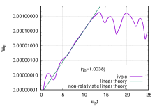
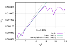
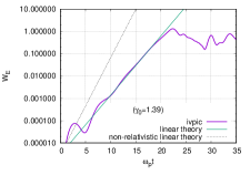
Figure 1: Time history of electric field energy ($W_{E}$) of relativistic two-stream instability simulations compared with linear theories.

We set up simulations with $V_{0}$ varying from non-relativistic to relativistic regimes. The domain size is set to be $L_{x}=2\pi d_{e}$, where $d_{e}$ is electron skin depth, with $N_{x}=32$ cells, $N_{pc}=200$ particles per cell. We employ a time step $\Delta t=0.99\Delta x/c$. The boundary conditions are periodic. Figure 1 shows the simulation results. We see that, in the non-relativistic regime ($\Gamma\simeq 1$), the simulation linear growth rate matches well with both Eq. 44 and the non-relativistic one, given by:

$$\textrm{Im}[\omega_{nr}]=\omega_{p}/2.$$ (45)

As $V_{0}$ increases, the relativistic lowering of the growth rate is more noticeable, as expected from the $\Gamma^{-3}$ scaling. For $\Gamma=1.39$, the relativistic growth rate decreases by a factor of $\sim 0.37$. In both weakly and strongly relativistic simulations, the change of the growth rate is very well captured.

4.2 Weibel instability

We use the Weibel instability to test the long time-scale conservation properties of the algorithm. The simulation is performed in a periodic 1D domain of $L_{x}=10d_{e}$ . We employ $N_{x}=64$ cells, $N_{pc}=200$ number of particles per cell, and a time step $\Delta t=0.99\Delta x/c$. Thermal temperatures of both electrons and ions are set to $v_{th,x}=0.1c$ and $v_{th,y,z}=0.3c$, respectively. The cell size is about 3 Debye lengths along $x$ at $t=0$. The mass ratio is set to $m_{i}/m_{e}=1836$. The boundary conditions are periodic.

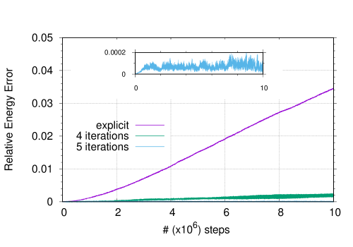
Figure 2: History of total energy conservation errors in long-term electron Weibel instability simulations. Energy conservation improves with increasing number of iterations. The insert shows the relative energy error of semi-implicit simulation with 5 iterations.

We consider energy conservation first. Fig. 2 shows the total energy error history as a function of the number of timesteps (up to $10^{7}$) for both explicit and semi-implicit simulations with different number of nonlinear iterations. It is worth noting that the original VPIC algorithm uses the method of Villasenor and Buneman [9], which has been shown to have much better energy conservation properties than the standard momentum-conserving schemes [34]. Strictly speaking, the discrete conservation law proposed in this study ensures conservation of total energy with the magnetic energy defined by $W_{B}=\frac{1}{2}\int d\mathbf{x}\mathbf{B}^{n+1/2}\cdot\mathbf{B}^{n-1/2}$, which is not always well-posed (see Appendix A for detailed discussion about $W_{B}$). However, $W_{B}$ is almost always well-posed except in pathological cases, as long as the light wave mode of interest are well resolved and the CFL condition is respected. On the other hand, $\hat{W}_{B}=\frac{1}{2}\int d\mathbf{x}\mathbf{B}^{n}\cdot\mathbf{B}^{n}$ at integer timesteps, which can be obtained from Eq. 14, is always positive and well-posed. We have found similar long-term behavior of both definitions (i.e., conserving one measure leads to bounded errors in the other). For the semi-implicit scheme, a few iterations have to be performed to maintain small energy errors. If a single iteration is used, which is equivalent to a first-order forward Euler method, the corresponding energy error would grow even faster than the explicit one (which is second-order accurate). Energy conservation errors decrease rapidly with the number of iterations. Figure 2 shows the relative error of total energy defined at integer timesteps (employing $\hat{W}_{B}$) up to $10^{7}$ timesteps. For this test, 5 nonlinear iterations are sufficient to maintain conservation errors at relatively low levels ($\sim 10^{-4})$.

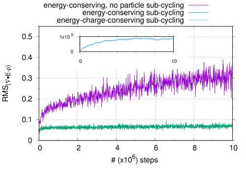
Figure 3: History of errors of Gauss’s law in long-term electron Weibel instability simulations. The insert shows the root-mean-square error of Gauss’s equation an semi-implicit simulation using the proposed energy- and charge-conserving algorithm.

Regarding charge conservation, Fig. 3 shows the root-mean-square of Gauss’s law evaluated on the mesh with different flavors of the semi-implicit solver, all of them energy conserving, but differing in the particle-push treatment. In particular, we consider three types of particle pusher: a single particle push per field step, a subcycled particle push but without special treatment at cell boundaries (with two subcycling steps), and the proposed single-step charge-conserving particle push. As discussed earlier (Sec. 3.5), Gauss’s law should be always satisfied everywhere if it is satisfied at $t=0$. Clearly, for the non-charge-conserving single-step particle-push case, Gauss’s law is violated and the errors accumulate secularly with the number of time steps. Particle sub-cycling improves the long-term behavior of error accumulation, but the level of error increases very quickly at the early stage of the simulation and saturates at relatively high level. With the energy- and charge- conserving scheme, Gauss’s law is satisfied with high accuracy during the simulation, and errors remain at a very low level ($\thicksim 10^{-5}$) .

4.3 Laser-plasma instabilities

We use the iVPIC code with a plane wave source at intensity $1.25x10^{15}\>\mathrm{W}/\mathrm{cm}^{2}$to simulate stimulated Raman scattering (SRS) and stimulated Brillouin scattering (SBS) in a single laser speckle , in a under-dense plasma ($n_{e}=0.05n_{cr}$) where $n_{cr}$ is the critical density, similar to that of Ref. [35]. The simulation is performed in a quasi-1D domain of size $320\times 0.11$ ($d_{e}^{2}$), with grid points $N_{x}\times N_{z}=7776\times 2$, and the number of particles per cell $N_{pc}=512$. timestep $\Delta t=0.98\,\Delta t_{CFL}$, where $\Delta t_{CFL}=\Delta x/\sqrt{2}c$ in two dimensions. The laser is polarized along $\hat{y}$ and the simulation is in the $\hat{x}-\hat{z}$ domain. We initiate the laser pulse by gradually ramping up the intensity at the $x=0$ boundary, and the laser propagates into the plasma. We employ absorbing boundary conditions for fields, and absorbing boundary conditions in $x$ and periodic in $z$ for particles. The laser speckle is modeled as a Gaussian laser pulse polarized along the $y$ direction. The same setup is simulated with both VPIC and iVPIC. Figure 4 shows the backscatter reflectivity ($r=1-$measured Poynting flux/Laser Poynting flux) obtained at $x=0$ from the quasi-1D simulation as a function of time. Except for some differences in the fluctuations that are sensitive to the thermal noise and random number seeds used, the instantaneous and running time-averaged the reflectivities agree well between VPIC and iVPIC. The two simulations reproduce both the bursty nature of SRS in the electron trapping regime at early times (t < 7 ps) as well as the transition to SBS at late times (t > 7 ps). Although differences are observed in the timing and amplitude of the individual bursts (which are known to be sensitive to the properties of the noise inherent to particle simulations), excellent agreement is found in the levels of time-averaged reflectivity between VPIC and iVPIC as well as the timing of the transition from SRS to SBS.

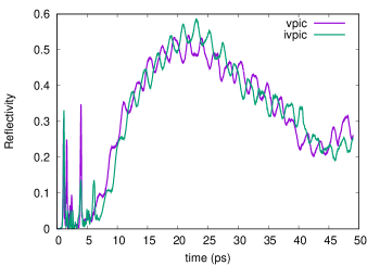
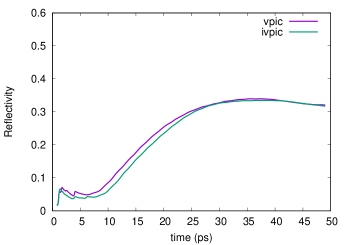
Figure 4: History of reflectivity in simulations with both VPIC and iVPIC (using 5 field-particle iterations). Left: instantaneous reflectivity averaged over laser period. Right: running time-averaged reflectivity (by $\frac{1}{T}\int_{0}^{T}r(t)dt$).

5 Discussion and summary

We have developed the first low-dispersion, energy- and charge-conserving relativistic Vlasov-Maxwell PIC algorithm. It is semi-implicit, leap-frogging electromagnetic fields and time-centering the particle push. The light wave dispersion errors are the same as the standard explicit PIC [2], and lower than the previously proposed fully implicit scheme [14]. It has been known that the Yee scheme conserves the discrete energy of electromagnetic fields [36, 37]. We have extended such a principle to PIC by ensuring that the energy exchange between particles and fields is treated correctly. It requires nonlinear iteration between the electric field update in Ampere’s equation and the particle push, but the iteration is not stiff and converges very quickly with a simple Picard iterative scheme. To ensure simultaneous rigorous and automatic charge conservation, we have developed a novel particle push scheme that not only deals with particle cell crossings effectively without actually stopping the particle at cell boundaries, but also is exactly energy-conserving and directly revertible (i.e. can be solved explicitly [20]). The superior properties of the scheme have been demonstrated on three numerical examples of varying complexity and dimensionality, from electrostatic (two-stream) to fully electromagnetic (Weibel, SBS). At this point, without vectorization and careful optimization, each iteration in iVPIC is about 50% slower than an unvectorized explicit step, resulting in a slowdown of a factor of 6 when 4 iterations are taken. Future work will focus on the implementation of higher-order particle-mesh interpolations, and on the vectorization and optimization of the algorithm on modern architectures.

Appendix

Appendix A Well-posedness of magnetic energy definition

We address the question of whether the magnetic energy definition in Eq. 24 is well-posed or not, i.e., whether the energy is positive and provide a physically meaningful measure. We show that it is almost always well-posed when the CFL timestep is respected, and it is a second-order accurate approximation of the magnetic energy defined at integer time levels. We begin by expressing $\mathbf{B}^{n\pm 1/2}$ around time $n$ as:

$$\mathbf{B}^{n\pm 1/2}=\mathbf{B}^{n}\pm\frac{\Delta t}{2}\partial_{t}\mathbf{B}^{n},$$ (46)

to find:

$$W_{B}=\hat{W}_{B}-\frac{\Delta t^{2}}{8}\int d\mathbf{x}(\partial_{t}\mathbf{B}^{n})\cdot(\partial_{t}\mathbf{B}^{n}),$$ (47)

where we denote $W_{B}=\frac{1}{2}\int d\mathbf{x}\mathbf{B}^{n+1/2}\cdot\mathbf{B}^{n-1/2}$, and $\hat{W}_{B}=\frac{1}{2}\int d\mathbf{x}(B^{n})^{2}$. This proves second-order accuracy. However, a priori, the measure $W_{B}$ may not be positive, while $\hat{W}_{B}$ is. For simplicity, we first show that $W_{B}$ is almost always well-posed in a 1D analysis.

Assuming that the magnetic field varies as $e^{-i\omega t+ikx}$, where $\omega=\omega(k)$,the discrete Fourier transform may be written as

$$\mathbf{B}(x,t)=\frac{1}{N_{g}}\sum_{l=0}^{N_{g}-1}\mathbf{B}(\omega_{l},k_{l})e^{-i\omega_{l}t+ik_{l}x},$$ (48)

where $N_{g}$ is the number of grid points and $k_{l}=\frac{2\pi l}{L}$. Then, by applying the Fourier transform to $W_{B}$,

$$\sum_{h=0}^{N_{g}-1}\mathbf{B}^{n+\nicefrac{{1}}{{2}}}(x_{h})\cdot\mathbf{B}^{n-\nicefrac{{1}}{{2}}}(x_{h})^{*} =\frac{1}{N_{g}^{2}}\sum_{h=0}^{N_{g}-1}\sum_{l=0}^{N_{g}-1}\sum_{m=0}^{N_{g}-1}\mathbf{B}(\omega_{l},k_{l})\cdot\mathbf{B}(\omega_{k},k_{m})^{*}e^{i(k_{l}-k_{m})x_{h}}\Re\left[e^{-i(\omega_{l}t^{n+\nicefrac{{1}}{{2}}}-\omega_{m}t^{n-\nicefrac{{1}}{{2}}})}\right]$$

$$=\frac{1}{N_{g}^{2}}\sum_{l=0}^{N_{g}-1}\sum_{m=0}^{N_{g}-1}\mathbf{B}(\omega_{l},k_{l})\cdot\mathbf{B}(\omega_{k},k_{m})^{*}\Re\left[e^{-i(\omega_{l}t^{n+\nicefrac{{1}}{{2}}}-\omega_{m}t^{n-\nicefrac{{1}}{{2}}})}\right]\sum_{h=0}^{N_{g}-1}e^{i(k_{l}-k_{m})x_{h}}$$

$$=\frac{1}{N_{g}}\sum_{l=0}^{N_{g}-1}\mathbf{B}(\omega_{l},k_{l})\cdot\mathbf{B}(\omega_{l},k_{l})^{*}\cos(\omega_{l}\Delta t),$$ (49)

where the superscript $*$ denotes complex conjugate, and $\Re[]$ denotes the real part of a complex number. We have used the orthogonal property of Fourier modes:

$$\sum_{h=0}^{N_{g}-1}e^{i(k_{l}-k_{m})x_{h}}=N_{g}\delta_{lm}.$$ (50)

From the 1D light wave dispersion relation:

$$\left[\frac{\Delta_{h}}{c\Delta t}\right]^{2}\sin^{2}\left(\frac{\omega\Delta t}{2}\right)=\sin^{2}\left(\frac{k_{x}\Delta_{h}}{2}\right),$$ (51)

and using that $2\sin^{2}(\theta/2)=1-\cos(\theta)$, we find that:

$$\cos(\omega\Delta t)\geq\left[\frac{c\Delta t}{\Delta_{h}}\right]^{2}\text{$\cos$($k_{x}\Delta_{h}$),}$$ (52)

when $\frac{c\Delta t}{\Delta_{h}}\leq 1$ . Therefore:

$$\sum_{h=0}^{N_{g}-1}\mathbf{B}^{n+\nicefrac{{1}}{{2}}}(x_{h})\cdot\mathbf{B}^{n-\nicefrac{{1}}{{2}}}(x_{h})^{*}\geq\frac{1}{N_{g}}\left[\frac{c\Delta t}{\Delta_{h}}\right]^{2}\sum_{l=0}^{N_{g}-1}\mathbf{B}(\omega_{l},k_{l})\cdot\mathbf{B}(\omega_{l},k_{l})^{*}\text{$\cos$($k_{l}\Delta_{h}$).}$$ (53)

For the case of white noise (equal spectral content in all frequencies), it is easy to see that:

$$\frac{1}{N_{g}}\sum_{l=0}^{N_{g}-1}\mathbf{B}(\omega_{l},k_{l})\cdot\mathbf{B}(\omega_{l},k_{l})^{*}\cos(k_{l}\Delta_{h})=A\sum_{l=0}^{N_{g}-1}\cos(k_{l}\Delta_{h})=0,$$ (54)

where $A$ is a positive constant, and provided that $N_{g}$ is an even number. It follows that:

$$\sum_{h=0}^{N_{g}-1}\mathbf{B}^{n+\nicefrac{{1}}{{2}}}(x_{h})\cdot\mathbf{B}^{n-\nicefrac{{1}}{{2}}}(x_{h})^{*}\geq 0,$$ (55)

i.e., the magnetic energy is positive definite if the CFL constraint $\frac{\Delta tc}{\Delta_{h}}<1$ is respected. In general, simulations will have varying spectral content with frequency, but low-frequency, well-resolved modes will carry the most information, and therefore the white noise analysis is conservative. For a mode with more than four grid points per wavelength, $\cos(k_{l}\Delta_{h})>0$. Therefore, as long as the field energy is not dominantly associated with high $k$ (i.e. $\left|k\Delta_{h}\right|>\pi/2$) modes, the field energy defined from $\mathbf{B}^{n+1/2}\cdot\mathbf{B}^{n-1/2}$ will be positive.

The above analysis can be straightforwardly extended to multiple dimensions. Assume a uniform grid, i.e., $\Delta x=\Delta y=\Delta z=\Delta_{h}$, and $\frac{\Delta tc}{\Delta_{h}}\lesssim\frac{1}{\sqrt{d}}$, where $d$ is the number of dimensions. Using the numerical dispersion relation of the light wave in 3D, i.e.,

$$\left[\frac{\Delta_{h}}{c\Delta t}\right]^{2}\sin^{2}\left(\frac{\omega\Delta t}{2}\right)=\sin^{2}\left(\frac{k_{x}\Delta_{h}}{2}\right)+\sin^{2}\left(\frac{k_{y}\Delta_{h}}{2}\right)+\sin^{2}\left(\frac{k_{z}\Delta_{h}}{2}\right),$$ (56)

we find that:

$$\cos(\omega\Delta t)\geq\left[\frac{c\Delta t}{\Delta_{h}}\right]^{2}\text{$\left[\cos(k_{x}\Delta_{h})+\cos(k_{y}\Delta_{h})+\cos(k_{z}\Delta_{h})\right]$.}$$ (57)

Clearly, the field energy given by Eq. 24 is well-posed if it is well-posed in each direction.

Appendix B Equivalence of Villasenor and Buneman’s charge conservation scheme and the proposed one

The proposed current and charge density deposition scheme and cell-crossing scheme are exactly the same as Villasenor and Buneman’s [9]. The derivation presented in Sec. 3.3 appears to be new, however, and can be easily extended to higher-order splines [32]. Here we explicitly demonstrate the equivalence of the two schemes.

Assume that the particle trajectory is from $(x_{p}^{n},y_{p}^{n},z_{p}^{n})$ to $(x_{p}^{n+1},y_{p}^{n+1},z_{p}^{n+1})$, which lies within a single cell. We employed B-splines which are written as (letting $\Delta x=\Delta y=\Delta z=1$, and $x_{i}=y_{j}=z_{k}=0$, without loss of generality):

$$S_{0}(x_{i+\nicefrac{{1}}{{2}}}-x_{p}) =1,$$ (58)

$$S_{1}(x_{i}-x_{p}) =1-x_{p},$$ (59)

$$S_{1}(x_{i+1}-x_{p}) =x_{p},$$ (60)

and similarly in $y$ and $z$ directions.

We first show that Eq. 31 is trivally satisfied. Assuming that the particle is in a cell centered at ($i+\nicefrac{{1}}{{2}}$), we write the equation for the node ($i$) and $(i+1)$ respectively as

$$\mathrm{lhs} =\frac{(1-x_{p}^{n+1})-(1-x_{p}^{n})}{\Delta t}+v_{x}^{n+\nicefrac{{1}}{{2}}}\frac{1-0}{1}=0,$$ (61)

$$\mathrm{lhs} =\frac{x_{p}^{n+1}-x_{p}^{n}}{\Delta t}+v_{x}^{n+\nicefrac{{1}}{{2}}}\frac{0-1}{1}=0,$$ (62)

where we have used Eq. 15. A formal derivation can be found in Ref. [11].

Adopting similar notations as in Ref. [9], we denote $\Delta x_{p}=x_{p}^{n+1}-x_{p}^{n}$, $\Delta y_{p}=y_{p}^{n+1}-y_{p}^{n}$, $\Delta z_{p}=z_{p}^{n+1}-z_{p}^{n}$, and $\bar{\xi}=(x_{p}^{n+1}+x_{p}^{n})/2$, $\bar{\eta}=(y_{p}^{n+1}+y_{p}^{n})/2$, $\bar{\zeta}=(z_{p}^{n+1}+z_{p}^{n})/2$, Eqs. 27-30 for the node $(i+1,j+1,k+1)$ are written as

$$\rho_{p,i+1,j+1,k+1}^{n+1} =q_{p}(\bar{\xi}+\frac{1}{2}\Delta x_{p})(\bar{\eta}+\frac{1}{2}\Delta y_{p})(\bar{\zeta}+\frac{1}{2}\Delta z_{p}),$$ (63)

$$\rho_{p,i+1,j+1,k+1}^{n} =q_{p}(\bar{\xi}-\frac{1}{2}\Delta x_{p})(\bar{\eta}-\frac{1}{2}\Delta y_{p})(\bar{\zeta}-\frac{1}{2}\Delta z_{p}),$$ (64)

$$j_{x,p,i+\nicefrac{{1}}{{2}},j+1,k+1}^{n+\nicefrac{{1}}{{2}}} =q_{p}(\frac{\Delta x_{p}}{\Delta t}\bar{\eta}\bar{\zeta}+\frac{1}{12}\Delta y_{p}\Delta z_{p}),$$ (65)

$$j_{y,p,i+1,j+\nicefrac{{1}}{{2}},k+1}^{n+\nicefrac{{1}}{{2}}} =q_{p}(\frac{\Delta y_{p}}{\Delta t}\bar{\zeta}\bar{\xi}+\frac{1}{12}\Delta z_{p}\Delta x_{p}),$$ (66)

$$j_{z,p,i+1,j+1,k+\nicefrac{{1}}{{2}}}^{n+\nicefrac{{1}}{{2}}} =q_{p}(\frac{\Delta z_{p}}{\Delta t}\bar{\xi}\bar{\eta}+\frac{1}{12}\Delta x_{p}\Delta y_{p}),$$ (67)

$$j_{x,p,i+\nicefrac{{3}}{{2}},j+1,k+1}^{n+\nicefrac{{1}}{{2}}} =0,$$ (68)

$$j_{y,p,i+1,j+\nicefrac{{3}}{{2}},k+1}^{n+\nicefrac{{1}}{{2}}} =0,$$ (69)

$$j_{z,p,i+1,j+1,k+\nicefrac{{3}}{{2}}}^{n+\nicefrac{{1}}{{2}}} =0,$$ (70)

and their substitutions into Eq. 26 yield

$$\Delta x_{p}\bar{\eta}\bar{\zeta}+\Delta y_{p}\bar{\zeta}\bar{\xi}+\Delta z_{p}\bar{\xi}\bar{\eta}=(\bar{\xi}+\frac{1}{2}\Delta x_{p})(\bar{\eta}+\frac{1}{2}\Delta y_{p})(\bar{\zeta}+\frac{1}{2}\Delta z_{p})-(\bar{\xi}-\frac{1}{2}\Delta x_{p})(\bar{\eta}-\frac{1}{2}\Delta y_{p})(\bar{\zeta}-\frac{1}{2}\Delta z_{p}),$$ (71)

which is exactly the same as Eq. 38 of Ref. [9] except for the subscript $p$ adopted in this study.

For trajectories across cell boundaries, the treatment is exactly the same as Villasenor and Buneman’s scheme, i.e., we split the trajectory into segments, each of which lies in one cell, and the above treatment applies.

References

- [1] K. Yee, “Numerical solution of initial boundary value problems involving Maxwell’s equations in isotropic media,” IEEE Transactions on antennas and propagation, vol. 14, no. 3, pp. 302–307, 1966.
- [2] C. K. Birdsall and A. B. Langdon, Plasma physics via computer simulation. CRC Press, 2004.
- [3] R. W. Hockney and J. W. Eastwood, Computer simulation using particles. CRC Press, 1988.
- [4] J. Dawson, “One-dimensional plasma model,” The Physics of Fluids, vol. 5, no. 4, pp. 445–459, 1962.
- [5] A. Hasegawa and H. Okuda, “One-dimensional plasma model in the presence of a magnetic field,” The Physics of Fluids, vol. 11, no. 9, pp. 1995–2003, 1968.
- [6] W. Lee, “Gyrokinetic approach in particle simulation,” The Physics of Fluids, vol. 26, no. 2, pp. 556–562, 1983.
- [7] C. Huang, V. K. Decyk, C. Ren, M. Zhou, W. Lu, W. B. Mori, J. H. Cooley, T. M. Antonsen Jr, and T. Katsouleas, “Quickpic: A highly efficient particle-in-cell code for modeling wakefield acceleration in plasmas,” Journal of Computational Physics, vol. 217, no. 2, pp. 658–679, 2006.
- [8] A. B. Langdon and B. F. Lasinski, “Electromagnetic and relativistic plasma simulation models,” Methods in Computational Physics, vol. 16, pp. 327–366, 1976.
- [9] J. Villasenor and O. Buneman, “Rigorous charge conservation for local electromagnetic field solvers,” Computer Physics Communications, vol. 69, no. 2-3, pp. 306–316, 1992.
- [10] T. Z. Esirkepov, “Exact charge conservation scheme for particle-in-cell simulation with an arbitrary form-factor,” Computer Physics Communications, vol. 135, no. 2, pp. 144–153, 2001.
- [11] G. Chen, L. Chacón, and D. C. Barnes, “An energy-and charge-conserving, implicit, electrostatic particle-in-cell algorithm,” Journal of Computational Physics, vol. 230, no. 18, pp. 7018–7036, 2011.
- [12] M. C. Pinto, S. Jund, S. Salmon, and E. Sonnendrücker, “Charge-conserving FEM–PIC schemes on general grids,” Comptes Rendus Mecanique, vol. 342, no. 10-11, pp. 570–582, 2014.
- [13] S. Markidis and G. Lapenta, “The energy conserving particle-in-cell method,” Journal of Computational Physics, vol. 230, no. 18, pp. 7037–7052, 2011.
- [14] G. Lapenta and S. Markidis, “Particle acceleration and energy conservation in particle in cell simulations,” Physics of Plasmas, vol. 18, no. 7, p. 072101, 2011.
- [15] G. Chen and L. Chacón, “A multi-dimensional, energy-and charge-conserving, nonlinearly implicit, electromagnetic Vlasov–Darwin particle-in-cell algorithm,” Computer Physics Communications, vol. 197, pp. 73–87, 2015.
- [16] L. Chacón and G. Chen, “A curvilinear, fully implicit, conservative electromagnetic PIC algorithm in multiple dimensions,” Journal of Computational Physics, vol. 316, pp. 578–597, 2016.
- [17] G. Lapenta, “Exactly energy conserving semi-implicit particle in cell formulation,” Journal of Computational Physics, vol. 334, pp. 349–366, 2017.
- [18] H. R. Lewis, “Energy-conserving numerical approximations for Vlasov plasmas,” Journal of Computational Physics, vol. 6, no. 1, pp. 136–141, 1970.
- [19] Y. Chen and G. Toth, “Gauss’s law satisfying energy-conserving semi-implicit particle-in-cell method,” arXiv preprint arXiv:1808.05745, 2018.
- [20] A. V. Higuera and J. R. Cary, “Structure-preserving second-order integration of relativistic charged particle trajectories in electromagnetic fields,” Physics of Plasmas, vol. 24, no. 5, p. 052104, 2017.
- [21] W. M. Seiler, Involution: The formal theory of differential equations and its applications in computer algebra, vol. 24. Springer Science & Business Media, 2009.
- [22] A. Taflove and S. C. Hagness, Computational electrodynamics: the finite-difference time-domain method. Artech house, 2005.
- [23] B. Marder, “A method for incorporating Gauss’ law into electromagnetic pic codes,” Journal of Computational Physics, vol. 68, no. 1, pp. 48–55, 1987.
- [24] A. B. Langdon, “On enforcing Gauss’ law in electromagnetic particle-in-cell codes,” Computer Physics Communications, vol. 70, no. 3, pp. 447–450, 1992.
- [25] C.-D. Munz, P. Omnes, R. Schneider, E. Sonnendrücker, and U. Voss, “Divergence correction techniques for Maxwell solvers based on a hyperbolic model,” Journal of Computational Physics, vol. 161, no. 2, pp. 484–511, 2000.
- [26] J.-L. Vay, “Simulation of beams or plasmas crossing at relativistic velocity,” Physics of Plasmas, vol. 15, no. 5, p. 056701, 2008.
- [27] R. Courant, K. Friedrichs, and H. Lewy, “On the partial difference equations of mathematical physics,” IBM journal of Research and Development, vol. 11, no. 2, pp. 215–234, 1967.
- [28] C. Sun and C. Trueman, “Unconditionally stable crank-nicolson scheme for solving two-dimensional Maxwell’s equations,” Electronics Letters, vol. 39, no. 7, pp. 595–597, 2003.
- [29] G. Sun and C. Trueman, “Unconditionally-stable FDTD method based on Crank-Nicolson scheme for solving three-dimensional Maxwell equations,” Electronics Letters, vol. 40, no. 10, pp. 589–590, 2004.
- [30] G. Chen and L. Chacón, “An energy-and charge-conserving, nonlinearly implicit, electromagnetic 1d-3v vlasov–darwin particle-in-cell algorithm,” Computer Physics Communications, vol. 185, no. 10, pp. 2391–2402, 2014.
- [31] J. D. Jackson, Classical electrodynamics. John Wiley & Sons, 2012.
- [32] A. Stanier, L. Chacón, and G. Chen, “A fully implicit, conservative, non-linear, electromagnetic hybrid particle-ion/fluid-electron algorithm,” Journal of Computational Physics, vol. 376, pp. 597–616, 2019.
- [33] K. J. Bowers, B. Albright, L. Yin, B. Bergen, and T. Kwan, “Ultrahigh performance three-dimensional electromagnetic relativistic kinetic plasma simulation,” Physics of Plasmas, vol. 15, no. 5, p. 055703, 2008.
- [34] A. Pukhov, “Three-dimensional electromagnetic relativistic particle-in-cell code VLPL (Virtual Laser Plasma Lab),” Journal of Plasma Physics, vol. 61, no. 3, pp. 425–433, 1999.
- [35] B. Albright, L. Yin, K. Bowers, and B. Bergen, “Multi-dimensional dynamics of stimulated brillouin scattering in a laser speckle: Ion acoustic wave bowing, breakup, and laser-seeded two-ion-wave decay,” Physics of Plasmas, vol. 23, no. 3, p. 032703, 2016.
- [36] R. Schuhmann and T. Weiland, “Conservation of discrete energy and related laws in the finite integration technique,” Progress In Electromagnetics Research, vol. 32, pp. 301–316, 2001.
- [37] F. Edelvik, R. Schuhmann, and T. Weiland, “A general stability analysis of FIT/FDTD applied to lossy dielectrics and lumped elements,” International Journal of Numerical Modelling: Electronic Networks, Devices and Fields, vol. 17, no. 4, pp. 407–419, 2004.