Equidistribution of primitive vectors, and the shortest solutions to their GCD equations

Abstract

We prove effective joint equidistribution of several natural parameters associated to primitive vectors in $\mathbb{Z}^{n}$, as the norm of these vectors tends to infinity. These parameters include the direction, the orthogonal lattice, and the length of the shortest solution to the associated $\gcd$ equation. We show that the first two parameters equidistribute w.r.t. the Haar measure on the corresponding spaces, which are the unit sphere and the space of unimodular rank $n-1$ lattices in $\mathbb{R}^{n}$ respectively. The main novelty is the equidistribution of the shortest solutions to the $\gcd$ equations: we show that, when normalized by the covering radius of the orthogonal lattice, the lengths of these solutions equidistribute in the interval $\left[0,1\right]$ w.r.t. a measure that is Lebesgue only when $n=2$, and non-Lebesgue otherwise. These equidistribution results are deduced from effectively counting lattice points in domains which are defined w.r.t. a generalization of the Iwasawa decomposition in simple algebraic Lie groups, where we apply a method due to A. Gorodnik and A. Nevo.

Contents

1. 1 Introduction
2. I From $\mathbb{Z}^{n}$ to $\operatorname{SL}_{n}\left(\mathbb{Z}\right)$
   1. 2 The Refined Iwasawa decomposition of $\operatorname{SL}_{n}\left(\mathbb{R}\right)$
      1. 2.1 Refining the Iwasawa decomposition
      2. 2.2 Explicit RI components of $g\in\operatorname{SL}_{n}\left(\mathbb{R}\right)$, and their interpretation
   2. 3 Fundamental domains representing spaces of lattices, shapes and directions
      1. 3.1 A set of representatives for the sphere
      2. 3.2 Fundamental domains for $\operatorname{SL}_{m}\left(\mathbb{Z}\right)$
      3. 3.3 Relation between fundamental domains and quotient spaces
   3. 4 Integral matrices representing primitive vectors
      1. 4.1 Correspondence between primitive vectors and matrices in $\operatorname{SL}_{n}\left(\mathbb{Z}\right)$
      2. 4.2 A fundamental domain for $\Gamma$ that captures the shortest solutions
   4. 5 Defining a counting problem
   5. 6 Simplifying the counting problem by restricting to compacts
   6. 7 Almost a proof for Theorems A and B
3. II Counting lattice points
   1. 8 Counting lattice points in well rounded families of sets inside Lie groups
      1. 8.1 A method for lattice points counting in Well rounded families
      2. 8.2 Plan of proof for Proposition 7.1
   2. 9 Well roundedness in subgroups of $A$
   3. 10 The Iwasawa roundomorphism
      1. 10.1 Effective Iwasawa decomposition
      2. 10.2 Effective Refined Iwasawa decomposition
      3. 10.3 Computing $f$ for the Iwasawa roundomorphism
   4. 11 The base sets
   5. 12 The family $\mathscr{Y}_{r(F_{n-1})}^{\,\alpha}$ is BLC
   6. 13 Concluding the proofs of the theorems

1 Introduction

An integral vector $v=\left(a_{1},\ldots,a_{n}\right)$ is called primitive if $\gcd\left(a_{1},\ldots,a_{n}\right)=1$. Equidistribution problems concerning primitive vectors first arose under the umbrella of Linnik type problems [Lin68, EH99, Duk03, Duk07, EMV13], a unifying name for questions that concern the distribution of the projections of integral vectors to the unit sphere. These projections can also be thought of as directions of primitive vectors, which we denote by $\hat{v}:=v/\left\|v\right\|$. Another equidistribution problem of primitive vectors concerns their orthogonal lattices $\Lambda_{v}:=\mathbb{Z}^{n}\cap v^{\perp}$, where $v$ is a primitive vector, and $v^{\perp}$ is its orthogonal hyperplane. Note that one can achieve a one-to-one correspondence between primitive vectors and their orthogonal lattices by either identifying $v$ with $-v$, or by choosing an orientation on the lattices $\Lambda_{v}$; we opt for the latter. With this one-to-one correspondence in mind, we associate to each primitive vector the shape of the lattice $\Lambda_{v}$, which is the equivalence class of rank $n-1$ lattices in $\mathbb{R}^{n}$ that can be obtained from $\Lambda_{v}$ by an orientation preserving linear transformation, i.e. by a rotation and multiplication by a positive scalar. The equidistribution of shapes of $\Lambda_{v}$, denoted $\operatorname{shape}\left(\Lambda_{v}\right)$, in the finite volume space

$$\mathcal{X}_{n-1}:=\operatorname{SO}_{n-1}\left(\mathbb{R}\right)\backslash\operatorname{SL}_{n-1}\left(\mathbb{R}\right)/\operatorname{SL}_{n-1}\left(\mathbb{Z}\right)$$

has been considered in [Mar10, Sch98]; the joint equidistribution of $\operatorname{shape}\left(\Lambda_{v}\right)$, along with the directions of $v$, denoted $\hat{v}$, has been studied in [AES16b, AES16a, EMSS16, ERW17].

Another equidistribution question for primitive vectors has been suggested by Risager and Rudnick in [RR09], and it concerns the normalized shortest solutions to $\gcd$ equations: given a primitive $v=\left(a_{1},\ldots,a_{n}\right)$, the gcd equation of $v$ is the Diophantine equation

$$a_{1}x_{1}+\cdots+a_{n}x_{n}=1,$$ (1.1)

whose set of solutions is the grid $w+\Lambda_{v}$, with $w$ being any solution to (1.1). Let $w_{v}$ denote the shortest solution to the equation (1.1) w.r.t. the $L^{2}$ norm. The length $\left\|w_{v}\right\|$ is unbounded as $\left\|v\right\|\to\infty$, so in order to formulate an equidistribution question for $\left\|w_{v}\right\|$, it should be normalized to a bounded quantity. Risager and Rudnick (see also [Tru13, HN16]) have considered the case of $n=2$, and showed that the quotients $\left\|w_{v}\right\|/\left\|v\right\|$ uniformly distribute in the interval $[0,\frac{1}{2}]$ as $\left\|v\right\|\to\infty$. This raises the question of what would be the analogous phenomenon in higher dimensions. It turns out that one can not expect equidistribution of $\left\|w_{v}\right\|/\left\|v\right\|$ when $n\geq 3$, since these quotients tend to zero on a full-density subset of the set of all $n$–primitive vectors, denoted $\mathbb{Z}_{\operatorname{prim}}^{n}$.

Theorem A.

There exists a subset $\mathcal{A}$ of $\mathbb{Z}_{\operatorname{prim}}^{n}$ with

$$\underset{R\to\infty}{\lim}\frac{\#(\mathcal{A}\cap B_{R})}{\#(\mathbb{Z}_{\operatorname{prim}}^{n}\cap B_{R})}=1,$$

where $B_{R}=\{v\in\mathbb{R}^{n}:\left\|v\right\|\leq R\}$, such that for every sequence $\{v_{m}\}\subset\mathcal{A}$, the quotients $\left\|w_{v_{m}}\right\|/\left\|v_{m}\right\|$ tend to zero as $m\to\infty$.

Indeed, the above theorem (as well as Corollary 1.2 below) suggests that in dimension greater than $2$, the “correct” normalization of the shortest solution is not by the norm of $v$. Hence, approaching Risager and Rudnick’s problem in higher dimensions consists in fact of three questions:

1. What is the correct normalization of the shortest solutions in dimension $n\geq 3$?

2. In which interval do the normalized shortest solutions fall?

3. With respect to which measure on this interval, if any, do the normalized shortest solutions equidistribute?

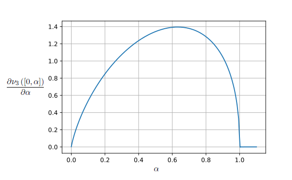
Figure 1: The density of $\nu_{3}$

In this paper we offer a complete solution to the problem of equidistribution of the normalized shortest solutions of $\gcd$ equations, answering all three questions above. We show that the correct normalization of $\left\|w_{v}\right\|$ is by the covering radius $\rho_{v}$ of the lattice $\Lambda_{v}$ (the covering radius of a lattice is the radius of a bounding sphere for its Dirichlet domain), and construct a measure $\nu_{n}$ with respect to which the quotients $\left\|w_{v}\right\|/\rho_{v}$ equidistribute in the interval $\left[0,1\right]$. It turns out that in general the measure $\nu_{n}$ on $\left[0,1\right]$ is non-uniform (see Figure 1 for the density function of $\nu_{3}$), except for the case of $n=2$: there, the measure $\nu_{2}$ is Lebesgue and the covering radius is $\rho_{v}=\left\|v\right\|/2$, hence we recover the result of Risager and Rudnick.

In fact we do more, and show that the equidistribution of $\left\|w_{v}\right\|/\rho_{v}$ occurs jointly with the uniform distribution of $\hat{v}$ in $\mathbb{S}^{n-1}$. We also obtain the previously known joint equidistribution of shapes $\operatorname{shape}\left(\Lambda_{v}\right)$ and directions $\hat{v}$ from the equidistribution of another parameter of $\Lambda_{v}$, that encodes information of both $\operatorname{shape}\left(\Lambda_{v}\right)$ and $\hat{v}$. Consider the space

$$\mathcal{L}_{n-1,n}:=\operatorname{SL}_{n}\left(\mathbb{R}\right)/\left(\left[\begin{array}[]{cc}\operatorname{SL}_{n-1}\left(\mathbb{Z}\right)&\mathbb{R}^{n-1}\\ 0_{1\times n}&1\end{array}\right]\times\left\{\left[\begin{array}[]{cc}\alpha^{-\frac{1}{n-1}}\operatorname{I}_{n-1}&0_{n\times 1}\\ 0_{1\times n}&\alpha\end{array}\right]:\alpha>0\right\}\right),$$

which is the space of homothety classes of $\left(n-1\right)$-lattices inside $\mathbb{R}^{n}$. We identify this space with the space of unimodular (i.e. covolume one) $\left(n-1\right)$-lattices inside $\mathbb{R}^{n}$,

$$\mathcal{L}_{n-1,n}\simeq\operatorname{SO}_{n}(\mathbb{R})\left[\begin{array}[]{cc}P_{n-1}&0\\ 0&1\end{array}\right]/\left[\begin{array}[]{cc}\operatorname{SL}_{n-1}\left(\mathbb{Z}\right)&0\\ 0&1\end{array}\right],$$ (1.2)

where $P_{n-1}<\operatorname{SL}_{n-1}(\mathbb{R})$ is the group of upper triangular matrices with positive diagonal entries. The identification is by associating to each equivalence class $\left[\Lambda\right]$ the unique representative of covolume one, which we also denote by $\left[\Lambda\right]$. The space $\mathcal{L}_{n-1,n}$ is canonically projected to $\mathcal{X}_{n-1}$ and to $\mathbb{S}^{n-1}$, by modding out from the left by $\operatorname{SO}_{n}(\mathbb{R})$ or by $\operatorname{SO}_{n-1}(\mathbb{R})\left[\begin{smallmatrix}P_{n-1}&0\\ 0&1\end{smallmatrix}\right]$ respectively, and the projections of $\left[\Lambda_{v}\right]$ to $\mathcal{X}_{n-1}$ and $\mathbb{S}^{n-1}$ are exactly $\operatorname{shape}\left(\Lambda_{v}\right)$ and $\hat{v}$.

From the equidistribution of $\left[\Lambda_{v}\right]$ in $\mathcal{L}_{n-1,n}$, we will also conclude the joint equidistribution of the directions $\hat{v}$ together with the projections of $\Lambda_{v}$ to the following space:

$$\mathcal{U}_{n-1}:=\operatorname{SL}_{n-1}\left(\mathbb{R}\right)/\operatorname{SL}_{n-1}\left(\mathbb{Z}\right),$$

which is the space of unimodular lattices of rank $n-1$. We denote these projections by $\left\llbracket\Lambda_{v}\right\rrbracket$ (this projection is in fact not canonical, and depends on a choice of coordinates that will be made in Section 2.2).

The equidistribution in the spaces $\mathcal{X}_{n-1}$, $\mathcal{U}_{n-1}$, $\mathcal{L}_{n-1,n}$ and $\mathbb{S}^{n-1}$ is a uniform distribution, namely w.r.t. a finite uniform invariant measure, which is unique up to a choice of normalization. We denote these measures by $\mu_{\mathcal{X}_{n-1}}$, $\mu_{\mathcal{U}_{n-1}}$, $\mu_{\mathcal{L}_{n-1,n}}$ and $\mu_{\mathbb{S}^{n-1}}$, and expand about them below, after the statement of our main result. The measure $\mu_{\mathbb{S}^{n-1}}$, for example, is the Lebesgue measure on the sphere.

The equidistribution of the quotients $\left\|w_{v}\right\|/\rho_{v}$ inside $[0,1]$ is, as we have already mentioned, not uniform. The proportion of primitive vectors $v$ for which the quotients $\left\|w_{v}\right\|/\rho_{v}$ fall within the interval $[0,\alpha]$ with $0\leq\alpha\leq 1$ is given by the map $\text{L}_{\alpha}:\mathcal{X}_{n-1}\to\mathbb{R}^{+}$ which is defined by associating to every $z\in\mathcal{X}_{n-1}$ the following quantity. Recall that $z\in\mathcal{X}_{n-1}$ is a unimodular lattice in $\mathbb{R}^{n-1}$ up to rotation. Recall also that the Dirichlet domain of a lattice is symmetric around the origin, and so the Lebesgue volume of $\mbox{Dir}(z)\cap B$, where $\mbox{Dir}(z)$ is the Dirichlet domain of any lattice in the class $z$ and $B$ is a ball centered at the origin, is independent of the choice of a representative from $z$. Let

$$\text{L}_{\alpha}(z)=\operatorname{Leb}(\mbox{Dir}(z)\cap B_{\alpha\rho\left(z\right)}),$$

where Leb is the Lebesgue measure, $\rho(z)$ is the covering radius of (any representative from) $z$, and $B_{\alpha\rho\left(z\right)}$ is an origin centered ball in $\mathbb{R}^{n-1}$ with radius $\alpha\rho\left(z\right)$.

Finally, we derive our equidistribution results by counting primitive vectors $v$ (resp. primitive $(n-1)$-lattices $\Lambda_{v}$) whose projections to the aforementioned spaces lie in subsets that have controlled boundary: this is a rather soft condition on the boundary of subsets of orbifolds that is defined explicitly in Section 3, and is met, e.g., when the boundary of the set is contained in a finite union of $C^{1}$ submanifolds of strictly lower dimension than the one of the orbifold. We refer to a set with controlled boundary as a boundary controllable set, or a BCS. Our main result is the following.

Theorem B.

Assume that $\Phi\subseteq\mathbb{S}^{n-1}$, $\mathcal{E}\subseteq\mathcal{X}_{n-1}$ $\widetilde{\mathcal{E}}\subseteq\mathcal{U}_{n-1}$ and $\Psi\subset\mathcal{L}_{n-1,n}$ are BCS’s.

1. The number of $v\in\mathbb{Z}_{\operatorname{prim}}^{n}$ with $\left\|v\right\|\leq e^{T}$, $\hat{v}\in\Phi$, $\operatorname{shape}\left(\Lambda_{v}\right)\in\mathcal{E}$ and $\left\|w_{v}\right\|/\rho_{v}\in\left[0,\alpha\right]$ is

   $$\frac{\mu_{\mathbb{S}^{n-1}}(\Phi)\cdot\int_{\mathcal{E}}\text{L}_{\alpha}(z)d\mu_{\mathcal{X}_{n-1}}\left(z\right)}{n\prod_{i=2}^{n}\zeta\left(i\right)}\cdot\frac{\prod_{i=1}^{n-2}\operatorname{Leb}(\mathbb{S}^{i})}{\iota\left(n-1\right)}\cdot e^{nT}+\text{error term}$$

   where

   $$\iota\left(m\right)=\left[\operatorname{SO}_{m}\left(\mathbb{R}\right):Z\left(\operatorname{SO}_{m}\left(\mathbb{R}\right)\right)\right]=\begin{cases}2&\mbox{if }m\mbox{ is even}\\ 1&\mbox{if }m\mbox{ is odd}\end{cases}.$$ (1.3)

2. The number of $v\in\mathbb{Z}_{\operatorname{prim}}^{n}$ with $\left\|v\right\|\leq e^{T}$, $\hat{v}\in\Phi$, $\left\llbracket\Lambda_{v}\right\rrbracket\in\widetilde{\mathcal{E}}$ and $\left\|w_{v}\right\|/\rho_{v}\in\left[0,\alpha\right]$ is

   $$\frac{\mu_{\mathbb{S}^{n-1}}(\Phi)\cdot\int_{\widetilde{\mathcal{E}}}\text{L}_{\alpha}(\pi_{{}_{\mathcal{U}\to\mathcal{X}}}\left(\tilde{z}\right))d\mu_{\mathcal{U}_{n-1}}\left(\tilde{z}\right)}{n\prod_{i=2}^{n}\zeta\left(i\right)}\cdot e^{nT}+\text{error term},$$

   where $\pi_{{}_{\mathcal{U}\to\mathcal{X}}}$ is the projection from $\mathcal{U}_{n-1}$ to $\mathcal{X}_{n-1}$.

3. The number of $v\in\mathbb{Z}_{\operatorname{prim}}^{n}$ with $\left\|v\right\|\leq e^{T}$, $\left[\Lambda_{v}\right]\in\Psi$ and $\left\|w_{v}\right\|/\rho_{v}\in\left[0,\alpha\right]$ is

   $$\frac{\int_{\Psi}\text{L}_{\alpha}(\pi_{{}_{\mathcal{L}\to\mathcal{X}}}\left(y\right))d\mu_{\mathcal{L}_{n-1,n}}\left(y\right)}{n\prod_{i=2}^{n}\zeta\left(i\right)}\cdot e^{nT}+\text{error term},$$

   where $\pi_{{}_{\mathcal{L}\to\mathcal{X}}}$ is the projection from $\mathcal{L}_{n-1,n}$ to $\mathcal{X}_{n-1}$.

The error term is $O_{\epsilon}(e^{nT\left(1-\tau_{n}+\epsilon\right)})$ with $\tau_{n}=\left\lceil\left(n-1\right)/2\right\rceil/4n^{2}$ for every $\epsilon>0$ when $\mathcal{E}$ (resp.  $\Psi$, $\widetilde{\mathcal{E}}$) is bounded, and $O_{\epsilon}(e^{nT\left(1-\eta_{n}\tau_{n}+\epsilon\right)})$ with $\eta_{n}=n^{2}/(2n^{3}-3n^{2}-2n+4)$ when it is not.

The lattice $\Lambda_{v}$ has covolume $\left\|v\right\|$ and it is primitive, where a lattice $\Lambda$ in $\mathbb{Z}^{n}$ is said to be primitive if it is of the form $V\cap\mathbb{Z}^{n}$, with $V$ being a linear subspace of $\mathbb{R}^{n}$ of dimension $\operatorname{rank}\left(\Lambda\right)$. Then, Theorem B can also be read as a counting result for primitive $(n-1)$–lattices, as their covolume tends to infinity.

The above theorem solves the question of equidistribution of the normalized shortest solutions; indeed, for $0\leq\alpha\leq 1$, let

$$\nu_{n}\left(\left[0,\alpha\right]\right)=\int_{z\in\mathcal{X}_{n-1}}\text{L}_{\alpha}(z)d\mu_{\mathcal{X}_{n-1}}\left(z\right).$$

The following is now straightforward from part (1) of Theorem B:

Corollary 1.1.

For primitive vectors $v\in\mathbb{Z}^{n}$ with $n\geq 2$, the normalized shortest solutions $\left\|w_{v}\right\|/\rho_{v}$ and the directions $\hat{v}$ jointly equidistribute as $\left\|v\right\|\to\infty$: the quotients $\left\|w_{v}\right\|/\rho_{v}$ inside $[0,1]$ w.r.t. $\nu_{n}$, and the directions $\hat{v}$ inside the unit sphere w.r.t. the Lebesgue measure.

As we have already mentioned, for the case of $n=2$ the above corollary recovers the result of Risager and Rudnick for uniform distribution of $\left\|w_{v}\right\|/\left\|v\right\|$ in the interval $[0,1/2]$. In particular, the ${n\choose 2}$ embeddings of $\mathbb{R}^{2}$ into $\mathbb{R}^{n}$ that are of the form

$$(x,y)\mapsto(0,\ldots,0,x,0,\ldots,0,y,0,\ldots 0)$$

give birth to ${n\choose 2}$ sequences of primitive vectors $v\in\mathbb{Z}^{n}$ for which the quotients $\left\|w_{v}\right\|/\left\|v\right\|$ uniformly distribute in the interval $[0,1/2]$ as $\left\|v\right\|\to\infty$. Combining this with Theorem A, we conclude:

Corollary 1.2.

For primitive vectors $v\in\mathbb{Z}^{n}$ with $n\geq 3$, there is no Borel measure on $\mathbb{R}$ w.r.t. which the quotients $\left\|w_{v}\right\|/\left\|v\right\|$ equidistribute as $\left\|v\right\|\to\infty$.

The measures $\mu_{\mathcal{X}_{n-1}}$, $\mu_{\mathcal{U}_{n-1}}$, $\mu_{\mathcal{L}_{n-1,n}}$ and $\mu_{\mathbb{S}^{n-1}}$.

The measure $\mu_{\mathbb{S}^{n-1}}$ is the Lebesgue measure on the sphere. The measures $\mu_{\mathcal{X}_{n-1}}$ and $\mu_{\mathcal{U}_{n-1}}$ are the unique Radon invariant measures arriving from a Haar measure on $\operatorname{SL}_{n-1}(\mathbb{R})$ that are normalized as follows: the $\mu_{\mathcal{U}_{n-1}}$ volume of $\mathcal{U}_{n-1}$ is

$$\prod_{i=2}^{n-1}\zeta\left(i\right),$$

and the $\mu_{\mathcal{X}_{n-1}}$-volume of $\mathcal{X}_{n-1}$ is

$$\iota\left(n-1\right)\prod_{i=2}^{n-1}\zeta\left(i\right)/(\prod_{i=1}^{n-2}\operatorname{Leb}(\mathbb{S}^{i})),$$

where $\iota:\mathbb{N}\to\left\{1,2\right\}$ was defined in (1.3). The justification for the volume of $\mathcal{U}_{n-1}$ is the computation in [Gar14] along our choice of Haar measure on $\operatorname{SL}_{n}\left(\mathbb{R}\right)$ that is explained in Subsection 2.1. This choice determines the volumes of $\mathcal{X}_{n-1}$, as shown in Lemma 3.9. On $\mathcal{L}_{n-1,n}$, however there is no invariant measure induced from $\operatorname{SL}_{n}(\mathbb{R})$, and instead we view this space as the quotient in (1.2), where a submanifold of $\operatorname{SL}_{n}(\mathbb{R})$ quotiented by a discrete group. This submanifold supports a transitive action of the product group $\operatorname{SO}_{n}(\mathbb{R})\times\left[\begin{smallmatrix}P_{n-1}&0\\ 0&1\end{smallmatrix}\right]$, and $\mu_{\mathcal{L}_{n-1,n}}$ is the unique Radon measure that is invariant under this action and satisfies that the $\mu_{\mathcal{L}_{n-1,n}}$-volume of $\mathcal{L}_{n-1,n}$ is the product of volumes of $\mathbb{S}^{n-1}$ and $\mathcal{U}_{n-1}$.

Comparison with previous work.

Let us comment on related work that preceded the theorem above. As already mentioned, equidistribution of the $\left\|w_{v}\right\|/\frac{1}{2}\left\|v\right\|$ was known for $n=2$; it was first proved in [RR09], and effective versions were later established in [Tru13] and [HN16], where the error term coincides with the one of Theorem B for $n=2$. The equidistribution (in a non-effective manner) of shapes of primitive lattices of any rank was established in [Sch98]; the case of rank $n-1$ was also obtained in [Mar10], using a dynamical approach. Theorem B adds an error term (i.e. rate of convergence) to two of the aforementioned results, as well as the consideration of the projections to $\mathcal{U}_{n-1}$ and $\mathcal{L}_{n-1,n}$ (as apposed to just $\mathcal{X}_{n-1}$), and most importantly, the equidistribution related to the $\gcd$ problem. Another significant addition is the fact that we allow the projections to the relevant spaces ($\mathcal{E}$, $\widetilde{\mathcal{E}}$, $\Psi$) to be unbounded; to this end, it is critical that the counting includes an error term, since it could be compromised to allow unboundedness. Our method can be used to consider the case of general co-dimension as well, which we will do in a forthcoming paper. Effective counting of primitive lattices was done in [Sch68],[Sch15], but the subsets $\mathcal{E}$ in the shape space were not general enough to deduce equidistribution. Joint equidistribution of shapes and directions has been studied, e.g. in [AES16b, AES16a, EMSS16], in the case where the primitive vectors $v$ are restricted to a large sphere $\left\|v\right\|=e^{T}$, as apposed to a large ball $\left\|v\right\|\leq e^{T}$, the latter being the case considered in Theorem B. The sphere case is of course much more delicate, and this is the reason why almost all existing results do not include an error term. The key to proving Theorem B is counting lattice points in the group $\operatorname{SL}_{n}\left(\mathbb{R}\right)$ w.r.t. the Iwasawa coordinates; in the context of counting points of discrete subgroups inside simple Lie groups w.r.t. a decomposition of the group, we mention [Goo83, GN12, GOS10, MMO14].

Outline of the paper.

The proof of Theorems A and B consist of two main ideas, and the paper is divided accordingly:

1. A reduction to a problem of counting lattice points in the group $\operatorname{SL}_{n}\left(\mathbb{R}\right)$ (Part I), which is done by finding “isomorphic” copies of the spaces $\mathcal{X}_{n-1}$, $\mathcal{U}_{n-1}$, $\mathcal{L}_{n-1,n}$, $\mathbb{S}^{n-1}$ inside $\operatorname{SL}_{n}\left(\mathbb{R}\right)$ (Section 3) and establishing a correspondence between primitive vectors $v$ (resp.  primitive lattices $\Lambda_{v}$) and integral matrices in $\operatorname{SL}_{n}\left(\mathbb{R}\right)$ (Section 4), such that the projections of the primitive lattices to the spaces $\mathcal{X}_{n-1}$ etc. will correspond to the projections of the integral matrices in their isomorphic copies. This converts Theorem B into a counting lattice points problem in $\operatorname{SL}_{n}\left(\mathbb{R}\right)$ (Section 5). A key role in this translation is played by a refinement of the Iwasawa coordinates of $\operatorname{SL}_{n}\left(\mathbb{R}\right)$, introduced in Section 2. In section 6 we simplify the counting problem by reducing to counting in a family of compact subsets of $\operatorname{SL}_{n}\left(\mathbb{R}\right)$, by providing a rather direct estimate for the number of lattice up to a given covolume that lie far up the cusp in the space of $(n-1)$-lattices. In the concluding section 7 of Part I we state Proposition 7.1, which formulates the final counting question in $\operatorname{SL}_{n}\left(\mathbb{R}\right)$ that is required in order to complete the proof Theorem B, and then use it to prove Theorems A and B.

2. Solving the counting problems (Part II ). This part is devoted to proving the aforementioned Proposition 7.1. The main ingredient is a method due to A. Gorodnik and A. Nevo [GN12], which concerns counting lattice points in increasing families $\left\{\mathcal{B}_{T}\right\}_{T>0}$ inside non-compact algebraic simple Lie groups. In Section 8 we describe this method, and sketch a plan for completing the proof of Proposition 7.1 according to it. In Sections 9, 10, 11, 12 we follow that plan, and the proofs are concluded in Section 13.

Notations for inequalities.

We will use the following conventions for inequalities. If $\underline{a}=\left(a_{1},\ldots,a_{n}\right)$ and $\underline{b}=\left(b_{1},\ldots,b_{n}\right)$ are two $n$-tuples of real numbers, we denote $\underline{a}\leq\underline{b}$ if $a_{i}\leq b_{i}$ for every $i=1,\ldots,n$. If $f$ and $g$ are two non-negative functions then we denote $f\ll g$ if there exists a positive constant $C$ and some $t_{0}$ such that for $t_{0}<t$ one has $f(t)\leq Cg(t)$. We denote $f\asymp g$ if $g\ll f\ll g$.

Acknowledgement.

This work was done when both authors were at IHES (Institut des Hautes Études Scientifiques, France), and we are grateful for the opportunity to work there, and for the outstanding hospitality. The authors are also grateful to Nadav Horesh for his help with numerical estimations for the measure $\nu_{3}$, and to Ami Paz for his help with preparing the figures. We would also like to thank Barak Weiss and Amos Nevo for helpful discussions in early stages of the project, and to Micheal Bersudsky for referring us to Schmidt’s work on effective counting of primitive lattices.

Part I From $\mathbb{Z}^{n}$ to $\operatorname{SL}_{n}\left(\mathbb{Z}\right)$

2 The Refined Iwasawa decomposition of $\operatorname{SL}_{n}\left(\mathbb{R}\right)$

2.1 Refining the Iwasawa decomposition

Set $G:=\operatorname{SL}_{n}\left(\mathbb{R}\right)$ and let $K$ be $\operatorname{SO}_{n}\left(\mathbb{R}\right)$, $A$ the diagonal subgroup in $G$, and $N$ the subgroup of upper unipotent matrices. Then, $G=KAN$ is the Iwasawa decomposition of $G$. Consider yet another subgroup of $G$,

$$G^{\prime\prime}:=\left[\begin{array}[]{c|c}\operatorname{SL}_{n-1}\left(\mathbb{R}\right)&\begin{array}[]{c}0\\ \underset{}{\vdots}\end{array}\\ \hline\cr\begin{array}[]{ccc}0&\cdots&0\end{array}&1\end{array}\right],$$

which is clearly an isomorphic copy of $\operatorname{SL}_{n-1}\left(\mathbb{R}\right)$ inside $G$. Write $G^{\prime\prime}=K^{\prime\prime}A^{\prime\prime}N^{\prime\prime}$ for the Iwasawa decomposition of $G^{\prime\prime}$, i.e.

$$K^{\prime\prime} := K\cap G^{\prime\prime}=\left[\begin{array}[]{c|c}\operatorname{SO}_{n-1}\left(\mathbb{R}\right)&\begin{array}[]{c}0\\ 0\end{array}\\ \hline\cr\begin{array}[]{cc}0&0\end{array}&1\end{array}\right],$$

$$A^{\prime\prime} := A\cap G^{\prime\prime}=\operatorname{diag}\left(\alpha_{1},\ldots,\alpha_{n-1},1\right)\text{ with }\alpha_{1}\cdots\alpha_{n-1}=1,$$

$$N^{\prime\prime} := N\cap G^{\prime\prime}=\left[\begin{array}[]{c|c}\begin{array}[]{c}\text{upper unipotent}\\ \text{of order $n-1$}\end{array}&\begin{array}[]{c}0\\ 0\end{array}\\ \hline\cr\begin{array}[]{cc}0&0\end{array}&1\end{array}\right].$$

The crux of the RI decomposition is that it completes the Iwasawa decomposition of $G^{\prime\prime}$ to the Iwasawa decomposition of $G$. For this we define $K^{\prime},A^{\prime},N^{\prime}$ that complete $K^{\prime\prime},A^{\prime\prime},N^{\prime\prime}$ to $K$, $A$ and $N$ respectively. Define

$$N^{\prime}:=\left[\begin{array}[]{c|c}\operatorname{I}_{n-1}&\mathbb{R}^{n-1}\\ \hline\cr\begin{array}[]{cc}0&0\end{array}&1\end{array}\right],\quad A^{\prime}:=\left[\begin{array}[]{c|c}a^{-\frac{1}{n-1}}\operatorname{I}_{n-1}&\begin{array}[]{c}0\\ 0\end{array}\\ \hline\cr\begin{array}[]{cc}0&0\end{array}&a\end{array}\right]$$

and note that $N=N^{\prime\prime}N^{\prime}$, $A=A^{\prime\prime}A^{\prime}$, and that $A^{\prime}$ is a one-parameter subgroup of $A$ which commutes with $G^{\prime\prime}$. Fix a transversal $K^{\prime}$ of the diffeomorphism $K/K^{\prime\prime}\to\mathbb{S}^{n-1}$ with the following property:

Condition 2.1.

If $\Phi\subseteq\mathbb{S}^{n-1}$ and $\Phi^{\prime\prime}\subseteq K^{\prime\prime}$ are BCS, then so does $\Phi^{\prime\prime}K_{\Phi}^{\prime}\subseteq K$, where $K_{\Phi}$ is the inverse image of $\Phi$ in $K^{\prime}$.

The existence of such a transversal $K^{\prime}$ is proved in Lemma 3.4. Let

$$P^{\prime\prime}:=A^{\prime\prime}N^{\prime\prime}\text{ and }Q:=KP^{\prime\prime};$$

note that $Q$ is not a group, but that it is a smooth manifold that is diffeomorphic to the group $K\times P^{\prime\prime}$. The RI decomposition is given by

$$G=K^{\prime}G^{\prime\prime}A^{\prime}N^{\prime}=K^{\prime}K^{\prime\prime}A^{\prime\prime}A^{\prime}N^{\prime\prime}N^{\prime},$$

and we also have $G=QA^{\prime}N^{\prime}$.

Parameterizations of the RI components.

Clearly the groups $A,A^{\prime},A^{\prime\prime}$ and $N,N^{\prime},N^{\prime\prime}$ are parameterized by the Euclidean spaces of the corresponding dimensions. For $t\in\mathbb{R}$, $\underline{s}=\left(s_{1},\ldots,s_{n-1}\right)\in\mathbb{R}^{n-2}$ and $\underline{x}\in\mathbb{R}^{n-1}$, we let $a_{t}^{\prime}:=\operatorname{diag}(e^{\frac{t}{n-1}}\operatorname{I}_{n-1},e^{-t})$, $a_{\underline{s}}^{\prime\prime}:=\operatorname{diag}(e^{-\frac{s_{1}}{2}},e^{\frac{s_{1-}s_{2}}{2}},\ldots,e^{\frac{s_{n-2}}{2}},1)$ and $n_{\underline{x}}^{\prime}=\left[\begin{smallmatrix}I_{n-1}&\underline{x}\\ 0&1\end{smallmatrix}\right]$. Similarly, since $K^{\prime}$ parameterizes the unit sphere $\mathbb{S}^{n-1}$, we let $k_{u}^{\prime}$ denote the element in $K^{\prime}$ corresponding to a unit vector $u\in\mathbb{S}^{n-1}$. In addition to the above, we will show in Section 3.3 that certain subsets of $Q$, $G^{\prime\prime}$ and $P^{\prime\prime}$ parameterize the spaces $\mathcal{L}_{n-1,n}$, $\mathcal{U}_{n-1}$ and $\mathcal{X}_{n-1}$. When an RI component $S$ (or a subset of it) parameterizes a space $X$, and $\mathcal{B}\subset X$ is a subset, we let $S_{\mathcal{B}}$ denote the image of $\mathcal{B}$ under the parameterization. For example, if ${\cal D}\subset\mathbb{R}^{n-1}$, then $N_{{\cal D}}^{\prime}$ denotes its image in $N^{\prime}$, namely the set of $n_{\underline{x}}^{\prime}$ where $\underline{x}\in{\cal D}$.

Measures on the RI components.

For every $S\subset G$ appearing as a component in the Iwasawa or Refined Iwasawa decompositions of $G$, we let $\mu_{S}$ denote a measure on $S$ as follows: $\mu_{K},\mu_{N}$ are Haar measures, and so do $\mu_{K^{\prime\prime}}$, $\mu_{N^{\prime\prime}}$, $\mu_{P^{\prime\prime}}$, $\mu_{G^{\prime\prime}},\mu_{G}$ and $\mu_{N^{\prime}}$. The measures $\mu_{N}$, $\mu_{N^{\prime}}$ and $\mu_{N^{\prime\prime}}$ are Lebesgue; as $N=N^{\prime\prime}\ltimes N^{\prime}$ and all three groups are unimodular, $\mu_{N}=\mu_{N^{\prime\prime}}\times\mu_{N^{\prime}}$. Since $K^{\prime}$ parameterizes $\mathbb{S}^{n-1}$, we can endow it with a measure $\mu_{K^{\prime}}$ that is the pullback of the Lebesgue measure on the sphere. We assume that the Haar measures $\mu_{K}$ and $\mu_{K^{\prime\prime}}$ are normalized such that $\mu_{K}=\mu_{K^{\prime\prime}}\times\mu_{K^{\prime}}$. Then, by choosing the measure of $K^{\prime\prime}$ to be $\prod_{i=1}^{n-2}\operatorname{Leb}(\mathbb{S}^{i})$, we have that the measure of $K$ is $\prod_{i=1}^{n-1}\operatorname{Leb}(\mathbb{S}^{i})$. The measures $\mu_{A},\mu_{A^{\prime}},\mu_{A^{\prime\prime}}$ are Radon measures such that

$$\mu_{A^{\prime}}=e^{nt}dt,\quad\mu_{A^{\prime\prime}}=\prod_{i=1}^{n-2}e^{-s_{i}}ds_{i}$$

as we compute in Example 9.4, and $\mu_{A}=\mu_{A^{\prime}}\times\mu_{A^{\prime\prime}}$ by Remark 9.3. Note that these measures are non-Haar. Since $Q$ is diffeomorphic to the group $K\times P^{\prime\prime}$, we endow it with the Haar measure on this group: $\mu_{Q}=\mu_{K}\times\mu_{P^{\prime\prime}}$. Since $\mu_{K}=\mu_{K^{\prime}}\times\mu_{K^{\prime\prime}}$, we also have that also $\mu_{Q}=\mu_{K^{\prime}}\times\mu_{G^{\prime\prime}}$. All in all, the Haar measure on $G$, which can be written in Iwasawa coordinates as $\mu_{G}=\mu_{K}\times\mu_{A}\times\mu_{N}$, (e.g. [Kna02, Prop. 8.43]), can be also decomposed according to the Refined Iwasawa coordinates:

$$\begin{array}[]{c}\mu_{G}=\mu_{K^{\prime}}\times\mu_{G^{\prime\prime}}\times\mu_{A^{\prime}}\times\mu_{N^{\prime}}=\mu_{Q}\times\mu_{A^{\prime}}\times\mu_{N^{\prime}}\\ =\mu_{K^{\prime}}\times\mu_{K^{\prime\prime}}\times\mu_{A^{\prime\prime}}\times\mu_{N^{\prime\prime}}\times\mu_{A^{\prime}}\times\mu_{N^{\prime}}\end{array}.$$ (2.7)

Where it should be clear from the context, we will occasionally denote $\mu$ instead of $\mu_{G}$

2.2 Explicit RI components of $g\in\operatorname{SL}_{n}\left(\mathbb{R}\right)$, and their interpretation

The following proposition reveals the role of the RI decomposition of $\operatorname{SL}_{n}\left(\mathbb{R}\right)$ in studying the parameters $\left\|v\right\|$, $\hat{v}$, $\left[\Lambda_{v}\right]$, $\left\llbracket\Lambda_{v}\right\rrbracket$ and $\operatorname{shape}\left(\Lambda_{v}\right)$ of a vector $v$. Let us observe that the projection $\left[\Lambda_{v}\right]$ to $\mathcal{U}_{n-1}$ is now well defined, following the choice of a transversal $K^{\prime}$, which determines a unique way to rotate any hyperplane in $\mathbb{R}^{n}$ to $\mbox{span}\{e_{1},\ldots,e_{n-1}\}\cong\mathbb{R}^{n-1}$.

It will be convenient to set the following notations: for any invertible matrix $g$, let $\Lambda_{g}$ denote the lattice spanned by the columns of $g$, and $\Lambda_{g}^{j}$ denote the lattice spanned by the first $j$ columns of $g$. Also, for $0\neq v\in\mathbb{R}^{n}$ define:

$$G_{v}=\left\{g=[v_{1}|\cdots|v_{n}]\in\operatorname{SL}_{n}\left(\mathbb{R}\right):v_{1}\wedge\cdots\wedge v_{n-1}=v\right\}.$$ (2.8)

Proposition 2.2.

Let $g=\left[v_{1}|\cdots|v_{n-1}|v_{n}\right]\in\operatorname{SL}_{n}\left(\mathbb{R}\right)$ and write $g=kan=qa_{t}^{\prime}n_{\underline{x}}^{\prime}$ with $q=k_{u}^{\prime}g^{\prime\prime}$ and $g^{\prime\prime}=k^{\prime\prime}a_{\underline{s}}^{\prime\prime}n^{\prime\prime}$. Let $w=v_{n}$, and $p^{\prime\prime}=a_{\underline{s}}^{\prime\prime}n^{\prime\prime}=\left[\begin{smallmatrix}z&0\\ 0&1\end{smallmatrix}\right]$. If $g\in G_{v}$, then the RI components of $g$ are as follows:

$$\begin{array}[]{ccccc}(i)&u&=&\hat{v}\\ (ii)&e^{t}&=&\left\|v\right\|\\ (iii)&e^{-\frac{s_{i}}{2}+\frac{it}{n-1}}&=&\operatorname{covol}(\Lambda_{g}^{i})\\ (iv)&\Lambda_{q}&\in&\left[\Lambda_{g}^{n-1}\right]\\ (v)&\Lambda_{g^{\prime\prime}}&\in&\left\llbracket\Lambda_{g}^{n-1}\right\rrbracket\\ (vi)&\Lambda_{z}&\in&\operatorname{shape}\left(\Lambda_{g}^{n-1}\right)\end{array}$$

and (vii) $\underline{x}=\left(x_{1},\ldots,x_{n-1}\right)$ is such that $w^{v^{\perp}}=\sum_{i=1}^{n-1}x_{i}v_{i}$.

The proof of this proposition requires two short lemmas regarding the elements of $G_{v}$.

Lemma 2.3.

For $g=\left[v_{1}|\cdots|v_{n-1}|v_{n}\right]\in\operatorname{SL}_{n}\left(\mathbb{R}\right)$, the following are equivalent:

1. $g\in G_{v}$.

2. The columns $\left\{v_{1},\ldots v_{n-1}\right\}$ form a basis of co-volume $\left\|v\right\|$ to $v^{\perp}$ such that $\left\{v_{1},\ldots,v_{n-1},v\right\}$ is a positively oriented basis w.r.t. the standard basis of $\mathbb{R}^{n}$.

3. $\left\langle v_{n},v\right\rangle=1$, and $\left\langle v_{i},v\right\rangle=0$ for $i=1,\ldots,n-1$.

Proof.

(1) $\iff$ (2) by definition. The direction (1) $\Longrightarrow$ (3) follows from

$$1=\det(g)=\langle(v_{1}\wedge\cdots\wedge v_{n-1}),v_{n}\rangle=\langle v,v_{n}\rangle.$$

Conversely, (3) implies $v=\alpha\cdot v_{1}\wedge\cdots\wedge v_{n-1}$ for some $\alpha\neq 0$, and that $\langle\alpha^{-1}v,v_{n}\rangle=\alpha^{-1}$. But since (as above) $1=\langle\alpha^{-1}v,v_{n}\rangle$, this forces $\alpha=1$. ∎

Lemma 2.4.

If $g\in G_{v}$, the last column of $g$ is $w$ and $w^{v^{\perp}}$ is the orthogonal projection of $w$ on the hyperplane $v^{\perp}$, then

$$w=w^{v^{\perp}}+\left\|v\right\|^{-2}\,v.$$

Proof.

Write $w=w^{v^{\perp}}+\alpha v$. By part (3) of Lemma 2.3, $1=\left\langle w,v\right\rangle=\langle w^{v^{\perp}}+\alpha v,v\rangle=\left\langle\alpha v,v\right\rangle$, hence $\alpha=\frac{1}{\left\|v\right\|^{2}}$. ∎

proof of Proposition 2.2.

Write $k=\left[\phi_{1}|\cdots|\phi_{n-1}|\phi_{n}\right]$. Since the columns of $k$ are the orthonormal basis obtained by the Gram-Schmidt algorithm on the columns of $g$, we have that $\mbox{span}\left\{\phi_{1},\ldots,\phi_{n-1}\right\}=\mbox{span}\left\{v_{1},\ldots,v_{n-1}\right\}=v^{\perp}$. By orthonormality and part (2) of Lemma 2.3, $\phi_{n}=\hat{v}=v/\left\|v\right\|$. Since $k$ and $k^{\prime}$ have the same last column, then $\hat{v}$ is also the last column of $k^{\prime}$, i.e. $k^{\prime}=k_{\hat{v}}^{\prime}$, which proves (i).

It is clear that if $a=\operatorname{diag}(a_{1},\ldots,a_{n})$, then ${\scriptstyle\prod_{1}^{i}}a_{j}=\left\|v_{1}\wedge\cdots\wedge v_{i-1}\wedge v_{i}\right\|=\operatorname{covol}(\Lambda_{g}^{i})$. Since $g\in G_{v}$, and $a$ has determinant $1$, we get that the last diagonal entry of $a$ (hence also of $a^{\prime}$) is $1/\left\|v\right\|$. This proves (ii) and (iii). In particular $a^{\prime}=\operatorname{diag}(\left\|v\right\|^{1/\left(n-1\right)},\dots,\left\|v\right\|^{1/\left(n-1\right)},\left\|v\right\|^{-1})$.

Write $g(n^{\prime})^{-1}(a^{\prime})^{-1}=k^{\prime}g^{\prime\prime}=q$; right multiplication by an element of $N^{\prime}$ does not change the first $n-1$ columns of $g$, and right multiplication by $(a^{\prime})^{-1}$ multiplies these columns by $\left\|v\right\|^{-1/\left(n-1\right)}$. This proves (iv), and (v), (vi) immediately follow.

Write $w$ as the sum of its projections to the orthogonal spaces $\mathbb{R}v$ and $v^{\perp}$: $w=w^{v}+w^{v^{\perp}}$. Observe that $g(n^{\prime})^{-1}=kp^{\prime\prime}a^{\prime}$. The last column of $kp^{\prime\prime}a^{\prime}$ is $\phi_{n}/\left\|v\right\|$, where from the calculation on $k^{\prime}$ we know that $\phi_{n}=\hat{v}$; by Lemma 2.4, we get that the last column of $kp^{\prime\prime}a^{\prime}$ is $w^{v}$. The last column of $g\left(n^{\prime}\right)^{-1}$ is $w-\sum_{i=1}^{n-1}x_{i}v_{i}$, so we conclude that $w-\sum_{i=1}^{n-1}x_{i}v_{i}=w^{v}=w-w^{v^{\perp}}$, which implies (vii). ∎

3 Fundamental domains representing spaces of lattices, shapes and directions

In this section we find “isomorphic” copies of the spaces $\mathcal{X}_{n-1}$, $\mathcal{U}_{n-1}$, $\mathcal{L}_{n-1,n}$, $\mathbb{S}^{n-1}$ inside $\operatorname{SL}_{n}\left(\mathbb{R}\right)$. The property we are after in these isomorphic copies, is that the images of sets satisfying a boundary condition, will also satisfy it. This boundary condition is the following:

Definition 3.1.

A subset $B$ of an orbifold $\mathcal{M}$ will be called boundary controllable set, or a BCS, if for every $x\in\mathcal{M}$ there is an open neighborhood $U_{x}$ of $x$ such that $U_{x}\cap\partial B$ is contained in a finite union of embedded $C^{1}$ submanifolds of $\mathcal{M}$, whose dimension is strictly smaller than $\dim\mathcal{M}$. In particular, $B$ is a BCS if its (topological) boundary consists of finitely many subsets of embedded $C^{1}$ submanifolds.

The goal of this section is to prove the following:

Proposition 3.2.

There exist full sets of representatives in $\operatorname{SL}_{n}\left(\mathbb{R}\right)$:

• $K^{\prime}\subset K$ parameterizing $\mathbb{S}^{n-1}\cong K^{\prime\prime}\backslash K$

• $\widetilde{F_{n-1}}\subset G^{\prime\prime}$ parameterizing $\mathcal{U}_{n-1}=G^{\prime\prime}/G^{\prime\prime}\left(\mathbb{Z}\right)$

• $F_{n-1}\subset P^{\prime\prime}$ parameterizing $\mathcal{X}_{n-1}\cong K^{\prime\prime}\backslash G^{\prime\prime}/G^{\prime\prime}\left(\mathbb{Z}\right)$

• $K^{\prime}\widetilde{F_{n-1}}\subset Q$ parameterizing $\mathcal{L}_{n-1,n}\cong Q/G^{\prime\prime}\left(\mathbb{Z}\right)$

that are BCS’s and with the properties that (i) a BCS is parameterized by a BCS and vice versa; for $K^{\prime}$, a product of BCS’s in $K^{\prime}$ and $K^{\prime\prime}$ is a BCS in $K$. (ii) The pullbacks of the invariant measures on the parameterized spaces to their set of representatives coincide with the measures that the sets of representatives inherent from their ambient manifolds: for all cases but $K^{\prime}$ it is the restriction of the measure $\mu_{S}$ on the ambient manifold, and for $K^{\prime}$ it is the measure $\mu_{K^{\prime}}$ defined in Subsection 2.1.

A full proof of Proposition 3.2 can be found in [HK20, Prop. 8.1] Here, we will only prove it fully for $K^{\prime}$ and $\mathbb{S}^{n-1}$ (this case is easier since $K^{\prime\prime}/K$ is compact), and for the remaining spaces we will settle for constructing fundamental domains that are BCS, with the property that the Haar measure restricted to them coincides with the unique (up to a scalar) invariant measure on the quotient (which is the space parameterized by the fundamental domain in question). We start by constructing sets of representatives for the sphere (Subsection 3.1), then for the spaces of lattices (Subsection 3.2), and we conclude with a partial proof of Proposition 3.2 in Subsection 3.3.

3.1 A set of representatives for the sphere

In order to construct a set of representatives $K^{\prime}$ for $\mathbb{S}^{n-1}$, we observe the following.

Fact 3.3.

Since $\partial\left(A\cup B\right),\partial\left(A\cap B\right)\subseteq\partial A\cup\partial B$, the union, intersection and subtraction of BCSs are in themselves BCS’s. Also, a finite product of BCSs is a BCS in the product of the ambient manifolds, and a diffeomorphic image of a BCS is a BCS.

Now the existence of a transversal $K^{\prime}$ for $\mathbb{S}^{n-1}$ is a consequence of the lemma below.

Lemma 3.4.

Let $K$ be a Lie group. Assume that $K^{\prime\prime}<K$ a closed subgroup such that the quotient space $K/K^{\prime\prime}$ is compact. There exists subset $K^{\prime}\subseteq K$ which is a BCS such that:

1. $\pi|_{K^{\prime}}:K^{\prime}\to K/K^{\prime\prime}$ is a bijection;

2. if $\Phi\subseteq K/K^{\prime\prime}$ and $\Phi^{\prime\prime}\subseteq K^{\prime\prime}$ are BCS, then the product $\underset{\subset K^{\prime}}{\underbrace{\pi|_{K^{\prime}}^{-1}(\Phi)}}\cdot\underset{\subset K^{\prime\prime}}{\underbrace{\Phi^{\prime\prime}}}$ in $K$ is also a BCS.

Proof of Lemma 3.4.

Since $\pi:K\to K/K^{\prime\prime}$ is a principal $K^{\prime\prime}$ fiber bundle, there exists an open covering $\left\{U_{\alpha}\right\}$ of $K/K^{\prime\prime}$ with $K^{\prime\prime}$-equivariant diffeomorphisms

$$\tau_{\alpha}:\pi^{-1}(U_{\alpha})\to U_{\alpha}\times K^{\prime\prime},$$

where $\tau_{\alpha}(x)=(\pi(x),*)$. We can assume that there is a BCS covering $\left\{W_{\alpha}\right\}$ of $K/K^{\prime\prime}$ such that $\overline{W_{\alpha}}\subseteq U_{\alpha}$ (e.g., by reducing to open balls contained in $U_{\alpha}$); by compactness, we may also assume that this covering is finite. Finally, by replacing every $W_{\alpha}$ with $W_{\alpha}\setminus\cup_{i=1}^{\alpha-1}W_{i}$, we may assume that the sets $W_{\alpha}$ are disjoint, maintaining the BCS property (Remark 3.3). Set

$$K^{\prime}=\sqcup_{\alpha}\tau_{\alpha}^{-1}\left(W_{\alpha}\times\operatorname{id}_{K^{\prime\prime}}\right)$$

(note that the interior is a manifold). Since the union is disjoint, $\pi|_{K^{\prime}}:K^{\prime}\to K/K^{\prime\prime}$ is a bijection. Moreover, since $W_{\alpha}$ is a BCS, then so does $W_{\alpha}\times\operatorname{id}_{K^{\prime\prime}}$, and then so does $\tau_{\alpha}^{-1}\left(W_{\alpha}\times\operatorname{id}_{K^{\prime\prime}}\right)$; by Remark 3.3, $K^{\prime}$ is a BCS.

Finally, by definition of $K^{\prime}$ one has that $k^{\prime}\in U_{\alpha}\cap K^{\prime}$ maps under $\tau_{\alpha}$ to $\left(\pi(k^{\prime}),\operatorname{id}_{K^{\prime\prime}}\right)$. If $\Phi\subseteq K/K^{\prime\prime}$ and $\Phi\subseteq K^{\prime\prime}$ then

$$\pi|_{K^{\prime}}^{-1}\left(\Phi\cap W_{\alpha}\right)\cdot\Phi=\tau_{\alpha}^{-1}\left(\left(\Phi\cap W_{\alpha}\right)\times\Phi\right),$$

where by Remark 3.3 the right hand side is a BCS. Then $\pi|_{K^{\prime}}^{-1}(\Phi)\cdot\Phi$ is a BCS, as a finite union of such. ∎

3.2 Fundamental domains for $\operatorname{SL}_{m}\left(\mathbb{Z}\right)$

We recall a construction for fundamental domains for the $\operatorname{SL}_{m}\left(\mathbb{Z}\right)$ action on $\operatorname{SL}_{m}\left(\mathbb{R}\right)$ and on $\operatorname{SO}_{m}\left(\mathbb{R}\right)\backslash\operatorname{SL}_{m}\left(\mathbb{R}\right)$), and list some of their properties.

Definition 3.5.

Let $\left\{v_{1},\ldots,v_{m}\right\}$ be a basis for $\mathbb{R}^{m}$, and let $\left\{\phi_{1},\ldots,\phi_{m}\right\}$ be the orthonormal basis obtained from it by the Gram-Schmidt orthogonalization algorithm. We say that $\left\{v_{1},\ldots,v_{m}\right\}$ is reduced if

1. the projection of $v_{j}$ to $V_{j-1}^{\perp}$ has minimal non-zero length $a_{j}$ (here $V_{0}=\left\{0\right\}$), where $V_{j-1}=\mbox{span}_{\mathbb{R}}\left\{v_{1},\ldots,v_{j-1}\right\}$;

2. the projection of $v_{j}$ to $V_{j-1}$ is $\sum_{i=1}^{j-1}n_{i,j}a_{i}\cdot\phi_{i}$ with $\left|n_{ij}\right|\leq\frac{1}{2}$ for all $i=1,\ldots,j-1$.

An $m\times m$ matrix with a reduced basis in its columns is also called reduced.

Observe that if a real $m\times m$ matrix $g$ is reduced, then it lies in $\operatorname{SL}_{m}\left(\mathbb{R}\right)$ and satisfies $g=kan$ where $k=[\begin{matrix}\phi_{1}&\cdots&\phi_{m}\end{matrix}]$, $a=\operatorname{diag}\left(a_{1},\ldots,a_{m}\right)$ and $n=\left[\begin{smallmatrix}1&n_{i,j}\\ 0&1\end{smallmatrix}\right]$, with $\phi_{j}$, $a_{j}$ and $n_{i,j}$ as in the definition above. In particular, whether $g$ is reduced or not, depends only on $an$. By the work of Siegel [BM00], the set of reduced matrices contains a fundamental domain for the action of $\operatorname{SL}_{m}\left(\mathbb{Z}\right)$. A specific choice of such a domain was made by Schmidt [Sch98] (see also [Gre93]), and it is defined as follows; we will use the notation $\mbox{Sym}^{+}\left(\Lambda\right)$ for the group of orientation preserving isometries of $\Lambda$ (sometimes referred to a the “point group” of $\Lambda$).

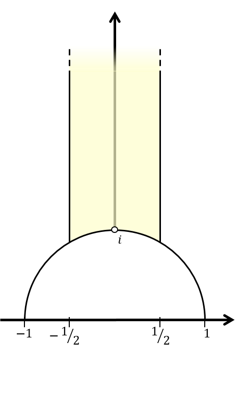
Figure 2: $F_{2}$: a fundamental domain for $\operatorname{SL}_{2}\left(\mathbb{Z}\right)$ in $P_{2}$ (the hyperbolic upper half plane).

Definition 3.6.

We let $\widetilde{F_{m}}\subset\operatorname{SL}_{m}\left(\mathbb{R}\right)=\operatorname{SO}_{m}\left(\mathbb{R}\right)P_{m}$, where $P_{m}$ is the subgroup consisting of upper triangular matrices, denote a choice of a fundamental domain lying inside the set of $g=kan\in\operatorname{SL}_{m}\left(\mathbb{R}\right)$ such that: (i) $g$ is reduced; (ii) $n_{1,j}\geq 0$ for $j>\iota\left(m\right)$ (see Notation (1.3)); (iii) $k$ lies inside a fundamental domain of $\mbox{Sym}^{+}\left(\Lambda_{an}\right)<\operatorname{SO}_{m}\left(\mathbb{R}\right)$, where $\Lambda_{an}$ is the lattice spanned by the columns of $an$. The projection of $\widetilde{F_{m}}$ to $P_{m}$ is denoted $F_{m}$ (Figure 2).

Note that conditions (i) and (ii) are on $an$, whereas condition (iii) is on $k$. Thus, the projection of $\widetilde{F_{m}}$ to $P_{m}\cong\operatorname{SO}_{m}\left(\mathbb{R}\right)\backslash\operatorname{SL}_{m}\left(\mathbb{R}\right)$ is a fundamental domain for the action of $\operatorname{SL}_{m}\left(\mathbb{Z}\right)$ on $\operatorname{SO}_{m}\left(\mathbb{R}\right)\backslash\operatorname{SL}_{m}\left(\mathbb{R}\right)$ that lies inside the set of triangular $m\times m$ matrices satisfying conditions (i) and (ii) in Definition 3.6, and the relation between $\widetilde{F_{m}}$ and $F_{m}$ is given by:

Proposition 3.7.

The relation between the fundamental domains $\widetilde{F_{m}}$ and $F_{m}$ is given by

$$\widetilde{F_{m}}=\bigcup_{z\in F_{m}}K_{z}\cdot z,$$

where $K_{z}$ is a fundamental domain for the finite group $\mbox{Sym}^{+}\left(\Lambda_{z}\right)$.

Note that $\widetilde{F_{m}}$ is not a product of $F_{m}\subset P_{m}$ with a subset of $\operatorname{SO}_{m}\left(\mathbb{R}\right)$, since different lattices $\Lambda_{z}$ have different point groups $\mbox{Sym}^{+}\left(\Lambda_{z}\right)$. However, there is only a finite number (that depends on $m$) of possible fibers, since there are finitely many possible symmetry groups for lattices in $\mathbb{R}^{m}$. Moreover, for generic $z$’s the point groups are identical:

Proposition 3.8 ([Sch98]).

For $z\in\operatorname{int}\left(F_{m}\right)$, $\mbox{Sym}^{+}\left(\Lambda_{z}\right)=Z\left(\operatorname{SO}_{m}\left(\mathbb{R}\right)\right)$, the center of $\operatorname{SO}_{m}\left(\mathbb{R}\right)$.

Thus suggests that for a full-measure set of $z\in F_{m}$, a uniform fiber in $K_{m}$ can be chosen; hence $\widetilde{F_{m}}$ can be approximated by $F_{m}$ times that generic fiber.

Lemma 3.9.

Let $G=\operatorname{SL}_{n}\left(\mathbb{R}\right)$ and $P<G$ the subgroup of upper triangular matrices. Assume $\widetilde{\mathcal{E}}\subseteq\mathcal{L}_{n}$ is the lift of $\mathcal{E}\subseteq\mathcal{X}_{n}$. If $\mathcal{E}$ is a BCS then $\widetilde{\mathcal{E}}$ is, and $\text{$\mu_{\mathcal{L}_{n}}$$(\widetilde{\mathcal{E}})$}=\mu_{\mathcal{X}_{n}}(\mathcal{E})\cdot{\scriptstyle\prod}_{i=1}^{n-1}\operatorname{Leb}(\mathbb{S}^{i})/\iota\left(n\right)$. Assume $\Psi\subseteq\mathcal{L}_{n-1,n}$ projects to $\widetilde{\mathcal{E}}\subseteq\mathcal{U}_{n-1}$ and $\Phi\subseteq\mathbb{S}^{n-1}$, in the sense that $Q_{\Psi}=K^{\prime}_{\Phi}G^{\prime\prime}_{\widetilde{\mathcal{E}}}$ (e.g. if $\Psi$ is the inverse image of $\widetilde{\mathcal{E}}$). If $\widetilde{\mathcal{E}}$ and $\Phi$ are BCS’s, then so is $Q_{\Psi}$, and $\mu_{\mathcal{L}_{n,n-1}}(\Psi)=\mu_{\mathcal{L}_{m}}(\widetilde{\mathcal{E}})\mu_{\mathbb{S}^{n-1}}(\Phi)$.

Proof.

By Proposition 3.7, $G_{\widetilde{\mathcal{E}}}=\bigcup_{z\in P_{\mathcal{E}}}K_{z}\cdot z$. Since there are only finitely many possible fibers, then by Proposition 3.8

$$G_{\widetilde{\mathcal{E}}}=(K_{\text{gen}}\cdot(P_{\mathcal{E}}\cap\operatorname{int}\left(F_{n}\right)))\cup(\bigcup_{i=1}^{q\left(n\right)}K_{z_{i}}\cdot\left\{z\in P_{\mathcal{E}}\cap\partial F_{m}:\mbox{Sym}^{+}\left(\Lambda_{z}\right)=\mbox{Sym}^{+}\left(\Lambda_{z_{i}}\right)\right\})$$

where $K_{\text{gen}}$ is the generic fiber and $\left\{z\in P_{\mathcal{E}}\cap\partial F_{n}:\mbox{Sym}^{+}(\Lambda_{z})=\mbox{Sym}^{+}(\Lambda_{z_{i}})\right\}$ is contained in $\partial F_{n}$, and is therefore a BCS of measure zero in $P$. Since the fibers in $\operatorname{SO}_{n}\left(\mathbb{R}\right)$ are BCS’s in $\operatorname{SO}_{n}\left(\mathbb{R}\right)$ due to Lemma 3.4, and since $P_{\mathcal{E}}\cap\operatorname{int}\left(F_{n}\right)$ is a BCS by Proposition 3.2 and Fact 3.3, and since $\operatorname{SO}_{n}\left(\mathbb{R}\right)\times P$ is diffeomorphic to $\operatorname{SL}_{n}\left(\mathbb{R}\right)$ with $\mu_{\operatorname{SL}_{n}\left(\mathbb{R}\right)}=\mu_{\operatorname{SO}_{n}\left(\mathbb{R}\right)}\times\mu_{P}$, we have that $G_{\widetilde{\mathcal{E}}}$ is a BCS in $\operatorname{SL}_{n}\left(\mathbb{R}\right)$ and has the same measure as $K_{\text{gen}}\cdot(P_{\mathcal{E}}\cap\operatorname{int}\left(F_{n}\right))$, which is $\mu_{\operatorname{SO}_{n}\left(\mathbb{R}\right)}(K_{\text{gen}})\cdot\mu_{P}(P_{\mathcal{E}})=\mu_{\operatorname{SO}_{n}\left(\mathbb{R}\right)}(\operatorname{SO}_{n}\left(\mathbb{R}\right))\mu_{P}(P_{\mathcal{E}})/\iota\left(n\right)=\mu_{P}(P_{\mathcal{E}})\cdot{\scriptstyle\prod}_{i=1}^{n-1}\operatorname{Leb}(\mathbb{S}^{i})/\iota\left(n\right)$ (recall choice of the volume of $\operatorname{SO}_{n}\left(\mathbb{R}\right)$ in Subsection 2.1). According to Proposition 3.2, which says that BCS’s and the measures in the “good” sets of representatives and in the spaces that they represent correspond, we get that we get that $\widetilde{\mathcal{E}}$ is a BCS and that $\text{$\mu_{\mathcal{U}_{n}}$$(\widetilde{\mathcal{E}})$}=\mu_{\mathcal{X}_{n}}(\mathcal{E})\cdot{\scriptstyle\prod}_{i=1}^{n-1}\operatorname{Leb}(\mathbb{S}^{i})/\iota\left(n\right)$.

The proof for $\Psi$ is a direct consequence of [HK20, Propositions 6.15 and 6.16] ∎

For future reference, we list some properties of $\widetilde{F_{m}},F_{m}$ that will be useful in the proof of our main theorem; in fact, the following applies to every reduced matrix, and in particular to the elements of $\widetilde{F_{m}},F_{m}$. The notations for $a_{j}$ and $V_{j}$ are as in Definition 3.5.

Lemma 3.10.

Suppose $g=kan$ is reduced and that its columns span a lattice $\Lambda$. Then

1. $n$ is a unipotent upper triangular matrix with non-diagonal entries in $\left[-1/2,1/2\right]$; in particular, $\left\|n^{\pm 1}\right\|,\left\|n^{\pm\operatorname{t}}\right\|\ll 1$.

2. $a=\operatorname{diag}\left(a_{1},\ldots,a_{m}\right)$ satisfies that $a_{1}\ll\cdots\ll a_{m}$. Specifically, $\frac{\sqrt{3}}{2}a_{j}\leq a_{j+1}$.

3. If $\lambda\in\Lambda$ satisfies $\lambda\notin V_{j-1}$, then $\left\|\lambda\right\|\geq\operatorname{dist}(\lambda,V_{j-1})\geq\operatorname{dist}(v_{j},V_{j-1})=a_{j}$.

4. If $x\in V_{j}$, then $\left\|ax\right\|\ll a_{j}\left\|x\right\|$.

3.3 Relation between fundamental domains and quotient spaces

In order to deduce that the invariant measures on the fundamental domains $K^{\prime}$, $\widetilde{F_{n-1}}$, $F_{n-1}$ etc. are the Haar measures on the spaces that they represent, we require the following result:

Theorem 3.11 ([Jüs18, Thm 2.2]).

Let $G$ be a unimodular Radon lcsc group with a Haar measure $\mu_{G}$, and let $\nu$ be a $G$-invariant Radon measure on an lcsc space $Y$. Assume that the $G$ action on $Y$ is strongly proper. Then there exists a unique Radon measure $\overline{\nu}$ on $G\backslash Y$ such that for all $f\in L^{1}\left(Y,\nu\right)$,

$$\int_{Y}f\left(y\right)d\nu\left(y\right)=\int_{G\backslash Y}\left(\int_{G}f\left(gy\right)d\mu_{G}\left(g\right)\right)d\overline{\nu}\left(Gy\right).$$

Proof of Proposition 3.2.

By construction, $K^{\prime}$, $\widetilde{F_{n-1}}$ and $F_{n-1}$ are sets of representatives for $\mathbb{S}^{n-1}$, $\mathcal{U}_{n-1}$ and $\mathcal{X}_{n-1}$ respectively, and $K^{\prime}\subset K$ is a BCS according to Lemma 3.4. $F_{n-1}\subset P^{\prime\prime}$ is a BCS since its boundary is contained in a finite union of lower-dimeansional manifolds in $P^{\prime\prime}$ (see [Sch98, pp. 48-49], and $\widetilde{F_{n-1}}\subset G^{\prime\prime}$ is a BCS by Lemma 3.9. Finally, $K^{\prime}\widetilde{F_{n-1}}\subset Q$, it is a set of representatives for $\mathcal{L}_{n-1,n}$ since

$$\operatorname{SL}_{n}\left(\mathbb{R}\right)/N^{\prime}G^{\prime\prime}\left(\mathbb{Z}\right)A^{\prime}\simeq K^{\prime}G^{\prime\prime}A^{\prime}N^{\prime}/G^{\prime\prime}\left(\mathbb{Z}\right)A^{\prime}N^{\prime}\simeq K^{\prime}G^{\prime\prime}/G^{\prime\prime}\left(\mathbb{Z}\right)$$

and $\widetilde{F_{n-1}}$ is a set of representatives for $G^{\prime\prime}/G^{\prime\prime}\left(\mathbb{Z}\right)\cong\mathcal{U}_{n-1}$. It is a BCS by Lemma 3.9. For part (i) of the proposition, a BCS in $\mathbb{S}^{n-1}$, $\mathcal{U}_{n-1}$, $\mathcal{X}_{n-1}$ or $\mathcal{L}_{n-1,n}$ is mapped to a BCS in $K^{\prime}$, $\widetilde{F_{n-1}}$, $F_{n-1}$ and $K^{\prime}\times\widetilde{F_{n-1}}$ respectively: for $K^{\prime}$ it holds because of Lemma 3.4, and for the remaining sets this is proved in [HK20, Prop. 8.1]. The correspondence of measures is a consequence of Theorem 3.11 above (but one can find more details in [HK20, Prop. 6.10]). ∎

4 Integral matrices representing primitive vectors

We begin in Subsection 4.1 by establishing a $1$ to $1$ correspondence between primitive vectors in $\mathbb{Z}^{n}$ and integral matrices in fundamental domains for the discrete subgroup defined as

$$\Gamma:=\left(N^{\prime}\rtimes G^{\prime\prime}\right)\left(\mathbb{Z}\right)=\left[\begin{array}[]{cc}\operatorname{SL}_{n-1}\left(\mathbb{Z}\right)&\mathbb{Z}^{n}\\ 0&1\end{array}\right].$$

Then, in Subsection 4.2, we define an explicit such fundamental domain in which the integral representative of a primitive vector $v$, has the shortest solution $w_{v}$ in its last column.

4.1 Correspondence between primitive vectors and matrices in $\operatorname{SL}_{n}\left(\mathbb{Z}\right)$

Recall $G_{v}$ was defined in Formula 2.8. We first prove:

Proposition 4.1.

If $\Omega\subset\operatorname{SL}_{n}\left(\mathbb{R}\right)$ is a fundamental domain for the right action of $\Gamma$, then there exists a bijection that depends on $\Omega$

$$\left(\mathbb{Z}^{n}\cap v^{\perp}\right)\leftrightarrow v\leftrightarrow\gamma_{v}\left(\Omega\right):=\mbox{the unique element in }\Omega\cap G_{v}\left(\mathbb{Z}\right),$$

between

$$\left\{\begin{subarray}{c}\mbox{primitive oriented}\\ \mbox{$\left(n-1\right)$-lattices in }\mathbb{Z}^{n}\end{subarray}\right\}\leftrightarrow\left\{\begin{subarray}{c}\mbox{primitive vectors}\\ \mbox{in }\mathbb{Z}^{n}\end{subarray}\right\}\leftrightarrow\left\{\begin{subarray}{c}\mbox{integral matrices}\\ \mbox{ in $\Omega$}\end{subarray}\right\}.$$

Proof.

The correspondence $\left(\mathbb{Z}^{n}\cap v^{\perp}\right)\leftrightarrow v$ is explained in the Introduction, and it suffices to show the correspondence $v\leftrightarrow\gamma_{v}\left(\Omega\right).$ We first claim that

$$G_{v}\cap\operatorname{SL}_{n}\left(\mathbb{Z}\right)\neq\left\{\emptyset\right\}\Longleftrightarrow v\in\mathbb{Z}^{n}\mbox{ primitive. }$$ (4.1)

The direction $\Longrightarrow$ is a consequence of (1)$\Rightarrow$(3) in Lemma 2.3. Conversely, if $v$ is primitive, then there exists $w\in\mathbb{Z}^{n}$ such that $\left\langle v,w\right\rangle=1$. Let $\left\{v_{1},\ldots,v_{n-1}\right\}$ be an integral basis for $v^{\perp}$ such that $\left\{v_{1},\ldots,v_{n-1},v\right\}$ is a positively oriented basis for $\mathbb{R}^{n}$. Then, by (3) $\Rightarrow$ (1) in Lemma 2.3, the resulting matrix $[v_{1}|\cdots|v_{n-1}|w]$ is in $G_{v}$. Since its columns are integral, it is also in $\operatorname{SL}_{n}\left(\mathbb{Z}\right)$.

Observe that $G_{v}$ is an orbit of the group $N^{\prime}\rtimes(G^{\prime\prime}\left(\mathbb{Z}\right))$, acting by right multiplication on $G=\operatorname{SL}_{n}\left(\mathbb{R}\right)$, and that $\Gamma$ is the subgroup of integral elements in this group. According to (4.1), $v\in\mathbb{Z}^{n}$ is primitive if and only if there exists an integral $\gamma$ in $G_{v}$. This is equivalent to all the points in the orbit $\gamma\cdot\Gamma$ being integral. Since $\Omega$ is a fundamental domain for $\Gamma$, the coset $\gamma\cdot\Gamma$ intersects $\Omega$ in a single point $\left\{\gamma_{v}\right\}=\Omega\cap(\gamma\cdot\Gamma)$. We claim that $\gamma\cdot\Gamma=G_{v}\left(\mathbb{Z}\right)$; indeed,

$$G_{v}\left(\mathbb{Z}\right)=G_{v}\cap\operatorname{SL}_{n}\left(\mathbb{Z}\right)=\left(\gamma\cdot N^{\prime}G^{\prime\prime}\right)\cap\operatorname{SL}_{n}\left(\mathbb{Z}\right)=\gamma\cdot(\left(N^{\prime}G^{\prime\prime}\right)\cap\operatorname{SL}_{n}\left(\mathbb{Z}\right))=\gamma\cdot\Gamma.$$

4.2 A fundamental domain for $\Gamma$ that captures the shortest solutions

Having shown that the primitive vectors in $\mathbb{R}^{n}$ correspond to integral matrices in a fundamental domain of $\Gamma$, we proceed to construct a specific such domain, with the property that every representative $\gamma_{v}$ has in its last column the shortest solution $w_{v}$ to the $\gcd$ equation of $v$. We begin with a more general (even if not as general as possible) construction for a fundamental domain of $\Gamma$; but first, a notation.

Notation 4.2.

For $g\in\operatorname{SL}_{n}\left(\mathbb{R}\right)$, we let $z^{g}$ denote the upper triangular $\left(n-1\right)\times\left(n-1\right)$ matrix such that the $P^{\prime\prime}$ component of $g$ is $\left[\begin{smallmatrix}z^{g}&1\\ 1&0\end{smallmatrix}\right]$.

Proposition 4.3.

Let $\widetilde{F}\subset\operatorname{SL}_{n-1}\left(\mathbb{R}\right)$ be a fundamental domain of $\operatorname{SL}_{n-1}\left(\mathbb{Z}\right)$, and $\mathscr{D}=\left\{{\cal D}\left(z\right)\right\}_{z\in F_{n-1}}$ be a family of fundamental domains for $\mathbb{Z}^{n-1}$ in $\mathbb{R}^{n-1}$. Then

$$\Omega=\Omega_{\mathscr{D}}:=\bigcup_{g^{\prime\prime}\in\widetilde{F}}K^{\prime}\cdot g^{\prime\prime}\cdot A^{\prime}\cdot N^{\prime}_{{\cal D}(z^{g^{\prime\prime}})}$$

is a fundamental domain for the action of $\Gamma$ on $\operatorname{SL}_{n}\left(\mathbb{R}\right)$ by multiplication from the right.

The proof is rather standard, and we skip it.

Remark 4.4.

Clearly, if all the domains ${\cal D}\left(z\right)$ are the same domain ${\cal D}$, then $\Omega$ is the product set $K^{\prime}G^{\prime\prime}_{\widetilde{F}}A^{\prime}N^{\prime}_{{\cal D}}$.

For $g$ in $\operatorname{SL}_{n}\left(\mathbb{R}\right)$, consider the linear map $L_{g}$ that sends the first $n-1$ columns of $g$ to the (ordered) standard basis for $\mathbb{R}^{n-1}$. Note that the $\left(n-1\right)$-lattice $\Lambda_{g}^{n-1}$, spanned by the first $n-1$ columns of $g$, is mapped under $L_{g}$ onto $\mathbb{Z}^{n-1}=\mbox{span}_{\mathbb{Z}}\left\{e_{1}\ldots,e_{n-1}\right\}$. As a result, a fundamental domain for $\Lambda_{g}^{n-1}$ in $v^{\perp}$ is mapped under $L_{g}$ onto a fundamental domain of $\mathbb{Z}^{n-1}$ in $\mathbb{R}^{n-1}$. We consider the image of the Dirichlet domain for $\Lambda_{g}^{n-1}$, which is $Y\left(z^{g}\right):=L_{g}(\mbox{Dir}(\Lambda_{g}^{n-1}))$. Note that indeed the right-hand side depends only on the $P^{\prime\prime}$ component of $g$: since $g=ka^{\prime}p^{\prime\prime}n^{\prime}$, then the RHS is $L_{n^{\prime}}L_{p^{\prime\prime}}L_{ka^{\prime}}(\mbox{Dir}(\Lambda_{g}^{n-1}))$. Now $L_{ka^{\prime}}$ acts as a rotation and multiplication by scalar such that $\Lambda_{g}^{n-1}$ maps to $\Lambda_{p^{\prime\prime}}^{n-1}=\Lambda_{z^{g}}$ and the Dirichlet domains map to one another. Since $L_{n^{\prime}}$ is identity map, then $L_{g}(\mbox{Dir}(\Lambda_{g}^{n-1}))$ equals $L_{p^{\prime\prime}}(\mbox{Dir}(\Lambda_{p^{\prime\prime}}^{n-1}))$. Then

$$\mathscr{Y}_{F_{n-1}}:=\left\{Y\left(z\right)\right\}_{z\in F_{n-1}}$$ (4.1)

is a family of fundamental domains for $\mathbb{Z}^{n-1}$ in $\mathbb{R}^{n-1}$, and so by Proposition 4.3 and by the notation for $K_{z}^{\prime\prime}$ appearing in Proposition 3.7, the following is a fundamental domain for $\Gamma$:

$$\Omega_{\operatorname{short}}:=\Omega_{\mathscr{Y}}=\bigcup_{g^{\prime\prime}\in\widetilde{F_{n-1}}}K^{\prime}\cdot g^{\prime\prime}\cdot A^{\prime}N_{Y\left(z^{g^{\prime\prime}}\right)}^{\prime}=\bigcup_{z\in F_{n-1}}K^{\prime}K_{z}^{\prime\prime}\cdot\underset{\in P^{\prime\prime}}{\underbrace{\left[\begin{smallmatrix}z&0\\ 0&1\end{smallmatrix}\right]}}\cdot A^{\prime}N_{Y\left(z\right)}^{\prime}.$$ (4.2)

Recall from Proposition 2.2 that

$$g=\left(|\cdots|w\right)\in G_{v}\cap\Omega(\mathscr{Y})\implies w^{v^{\perp}}\in L_{g}^{-1}(Y\left(z^{g}\right))\iff w^{v^{\perp}}\in\mbox{Dir}(\Lambda_{g}^{n-1}),$$

namely $w^{v^{\perp}}$ (such that $w=v/\left\|v\right\|^{2}+w^{v^{\perp}}$, see Lemma 2.4) is the shortest representative of the coset $w^{v^{\perp}}+\Lambda_{g}^{n-1}$ in the hyperplane $v^{\perp}$. This means that $w$ is the shortest representative of the coset $w+\Lambda_{g}^{n-1}$ (which lies in the affine hyperplane $\left\{u:\left\langle u,v\right\rangle=1\right\}$). As a result, for every primitive vector $v$, the representative $\gamma_{v}=G_{v}\left(\mathbb{Z}\right)\cap\Omega_{\operatorname{short}}$, has last column $w$ which is

$$w_{v} := \mbox{the shortest integral $w\;$which satisfies $\left\langle w,v\right\rangle=1$}.$$

The relation between the norm of $w_{v}$, which is what we are interested in for Theorems A and B, and between the norm of $w_{v}^{v^{\perp}}$, which is what is captured by $\Omega_{\operatorname{short}}$, is given by the following lemma.

Lemma 4.5.

If $\{v_{n}\}$ is a divergent sequence of primitive vectors, then

$$\underset{n\to\infty}{\lim}\left|\left\|w_{v_{m}}\right\|-\left\|w_{v_{m}}^{v_{m}^{\perp}}\right\|\right|=O(\left\|v_{m}\right\|^{-1}).$$

Proof.

By Lemma 2.4,

$$|\left\|w_{v_{m}}\right\|-\left\|w_{v_{m}}^{v_{m}^{\perp}}\right\||\leq\left\|w_{v_{m}}-w_{v_{m}}^{v_{m}^{\perp}}\right\|=\frac{1}{\left\|v_{m}\right\|}.$$

∎

5 Defining a counting problem

The goal of this section is to reduce the proof of Theorem B into a problem of counting integral matrices in subsets of $\operatorname{SL}_{n}\left(\mathbb{R}\right)$, and specifically of $\Omega_{\operatorname{short}}$. We begin by defining these subsets. First, consider the covering radius of the lattice spanned by the first $n-1$ columns:

$$\rho(\Lambda_{g}^{n-1}) = \mbox{radius of bounding circle for $\mbox{Dir}(\Lambda_{g}^{n-1})$}.$$

Clearly, the norm $\|w^{v^{\perp}}\|$ lies in the interval $[0,\rho(\Lambda_{g})]$, i.e.

$$\frac{\|w^{v^{\perp}}\|}{\rho\left(\Lambda_{g}\right)}\in\left[0,1\right].$$

We consider sub-families $\mathscr{Y}^{\,\alpha}\subseteq\mathscr{Y}$ for which this quotient is restricted to a sub-interval $\left[0,\alpha\right]$, with $0\leq\alpha\leq 1$. Let $B_{r}^{v^{\perp}}$ denote an origin-centered $n-1$ dimensional ball in $v^{\perp}$ whose radius is $r$. For $\alpha\in\left[0,1\right]$, let

$$Y^{\alpha}(z^{g}) = L_{g}(B_{\alpha\rho\left(\Lambda_{g}\right)}^{v^{\perp}}\cap\mbox{Dir}(\Lambda_{g}))$$

$$\mathscr{Y}_{F_{n-1}}^{\,\alpha} = \left\{Y^{\alpha}(z)\right\}_{z\in F_{n-1}}.$$ (5.1)

We now turn to define the subsets of $\Omega_{\operatorname{short}}$ such that the integral matrices inside them represent via the bijection $\gamma_{v}\leftrightarrow v$ the primitive vectors that are counted in Theorem B.

Notation 5.1.

For $T>0$, $\Phi\subseteq\mathbb{S}^{n-1}$, $\widetilde{\mathcal{E}}\subseteq\mathcal{U}_{n-1}$, $\mathcal{E}\subseteq\mathcal{X}_{n-1}$, $\Psi\subseteq\mathcal{L}_{n-1,n}$ and $\alpha\in\left[0,1\right]$, recall the notation in 4.2 and consider

$$\left(\Omega_{\operatorname{short}}\right)_{T}(\Phi,\mathcal{E},\alpha)=\,\Omega_{\operatorname{short}}\,\cap\,\left\{g=k^{\prime}k^{\prime\prime}p^{\prime\prime}a^{\prime}n^{\prime}:\begin{matrix}k^{\prime}\in K^{\prime}_{\Phi},a^{\prime}\in A^{\prime}_{\left[0,T\right]},\\ p^{\prime\prime}\in P^{\prime\prime}_{\mathcal{E}},n^{\prime}\in N^{\prime}_{Y^{\alpha}(z^{g})}\end{matrix}\right\}=\bigcup_{p^{\prime\prime}\in P^{\prime\prime}_{\mathcal{E}}}K^{\prime}_{\Phi}\cdot K_{z^{p^{\prime\prime}}}^{\prime\prime}\cdot p^{\prime\prime}\cdot A_{T}^{\prime}N^{\prime}_{Y^{\alpha}(z^{p^{\prime\prime}})},$$

$$\left(\Omega_{\operatorname{short}}\right)_{T}(\Phi,\widetilde{\mathcal{E}},\alpha)=\,\Omega_{\operatorname{short}}\cap\left\{g=k^{\prime}g^{\prime\prime}a^{\prime}n^{\prime}:\begin{matrix}k^{\prime}\in K^{\prime}_{\Phi},a^{\prime}\in A^{\prime}_{\left[0,T\right]},\\ g^{\prime\prime}\in G^{\prime\prime}_{\widetilde{\mathcal{E}}},n^{\prime}\in N^{\prime}_{Y^{\alpha}(z^{g})}\end{matrix}\right\}=\bigcup_{g^{\prime\prime}\in G^{\prime\prime}_{\widetilde{\mathcal{E}}}}K^{\prime}_{\Phi}\cdot g^{\prime\prime}\cdot A_{T}^{\prime}N^{\prime}_{Y^{\alpha}(z^{g^{\prime\prime}})},$$

and

$$\left(\Omega_{\operatorname{short}}\right)_{T}(\Psi,\alpha)=\,\Omega_{\operatorname{short}}\,\cap\,\left\{g=qa^{\prime}n^{\prime}:\begin{matrix}q\in Q_{\Psi},a^{\prime}\in A^{\prime}_{\left[0,T\right]},\\ n^{\prime}\in N^{\prime}_{Y^{\alpha}(z^{g})}\end{matrix}\right\}=\bigcup_{q\in Q_{\Psi}}q\cdot A_{T}^{\prime}N^{\prime}_{Y^{\alpha}(z^{q})}.$$

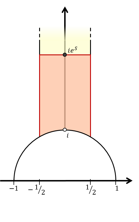
Figure 3: The domain $F_{2}^{S}$.

The following notation is for sets in $G$ whose $A^{\prime\prime}$ component is restricted to a compact box.

Notation 5.2.

For every $\underline{S}=(S_{1},\ldots,S_{n-2})>\underline{0}$ and a subset $\mathcal{B}\subset G$, let $\mathcal{B}^{\underline{S}}$ denote the subset $\mathcal{B}\cap\{g:\pi_{A_{i}^{\prime\prime}}\left(g\right)\leq S_{i}\,\forall i\}$, where $\pi_{A_{i}^{\prime\prime}}$ is the projection to the $A_{i}^{\prime\prime}$ component (see Figure 3 for $F_{2}^{S}$).

Recall from the Introduction that $\Lambda_{v}=\Lambda_{\gamma_{v}}^{n-1}$ and $\rho_{v}=\rho(\Lambda_{v}^{n-1})$. The following is now immediate from Proposition 4.1, Proposition 2.2, and the construction of $\Omega_{\operatorname{short}}$, and concludes the translation of Theorem B into a problem of counting lattice points in $\operatorname{SL}_{n}\left(\mathbb{R}\right)$:

Corollary 5.3.

Consider the correspondence $v\leftrightarrow\gamma_{v}$ where $\gamma_{v}=\left(G_{v}\left(\mathbb{Z}\right)\right)\cap\Omega_{\operatorname{short}}$. For $T>0$, $\Phi\subseteq\mathbb{S}^{n-1}$ $\widetilde{\mathcal{E}}\subseteq\mathcal{U}_{n-1}$ , $\mathcal{E}\text{$\subseteq\mathcal{X}_{n-1}$}$, $\Psi\subseteq\mathcal{L}_{n-1,n}$ and $\alpha\in\left[0,1\right]$:

1. The $\operatorname{SL}_{n}\left(\mathbb{Z}\right)$ matrices in $\left(\Omega_{\operatorname{short}}\right)_{T}(\Phi,\mathcal{E},\alpha)$ correspond under $\gamma_{v}\leftrightarrow v$ to the elements of

   $$\left\{v\in\mathbb{Z}^{n}\mbox{ primitive}:\left\|v\right\|\leq e^{T},\hat{v}\in\Phi,\operatorname{shape}\left(\Lambda_{v}\right)\in\mathcal{E},\|w^{v^{\perp}}\|/\rho_{v}\in\left[0,\alpha\right]\right\}.$$

2. The $\operatorname{SL}_{n}\left(\mathbb{Z}\right)$ matrices in $\left(\Omega_{\operatorname{short}}\right)_{T}(\Phi,\widetilde{\mathcal{E}},\alpha)$ correspond under $\gamma_{v}\leftrightarrow v$ to the elements of

   $$\left\{v\in\mathbb{Z}^{n}\mbox{ primitive}:\left\|v\right\|\leq e^{T},\hat{v}\in\Phi,\left\llbracket\Lambda_{v}\right\rrbracket\in\widetilde{\mathcal{E}},\|w^{v^{\perp}}\|/\rho_{v}\in\left[0,\alpha\right]\right\}.$$

3. The $\operatorname{SL}_{n}\left(\mathbb{Z}\right)$ matrices in $\left(\Omega_{\operatorname{short}}\right)_{T}(\Psi,\alpha)$ correspond under $\gamma_{v}\leftrightarrow v$ to the elements of

   $$\left\{v\in\mathbb{Z}^{n}\mbox{ primitive}:\left\|v\right\|\leq e^{T},\left[\Lambda_{v}\right]\in\Psi,\|w^{v^{\perp}}\|/\rho_{v}\in\left[0,\alpha\right]\right\}.$$

For the cases where $\mathcal{E}$ (resp.  $\widetilde{\mathcal{E}}$, $\Psi$) is the set parametertized by $F_{n-1}^{\underline{S}}$ (resp.  $\widetilde{F_{n-1}}^{\underline{S}}$, $K^{\prime}\widetilde{F_{n-1}}^{\underline{S}}$) with $\underline{S}=(S_{1},\dots,S_{n-2})$, then the condition $\operatorname{shape}\left(\Lambda_{v}\right)\in\mathcal{E}$ (resp. $\left\llbracket\Lambda_{v}\right\rrbracket\in\widetilde{\mathcal{E}}$, $\left[\Lambda_{v}\right]\in\Psi$) is equivalent to $\frac{\left\|\left(v_{1}\wedge\cdots\wedge v_{i}\right)\right\|}{\left\|v\right\|^{i/\left(n-1\right)}}\geq e^{-S_{i}/2}$ for every $1\leq i\leq n-2$.

6 Simplifying the counting problem by restricting to compacts

In the previous section we reduced the proof of Theorem B to counting $\operatorname{SL}_{n}\left(\mathbb{Z}\right)$ points inside the subsets $\left(\Omega_{\operatorname{short}}\right)_{T}$ as $T\to\infty$. These sets have the disadvantage of not being compact, despite their finite volume; this is apparent from the fact that they contain $A^{\prime\prime}$, which is unbounded. Since our counting method (described in Subsection 8.1) does not allow non-compact sets, the aim of this section is to reduce counting in $\left(\Omega_{\operatorname{short}}\right)_{T}$ to counting in a compact subset of it. Here we will allow a fundamental domain of $\Gamma$ as general as in Corollary 4.3, and not restrict just to $\Omega_{\operatorname{short}}$.

Notation 6.1.

Let $\Omega$ be a fundamental domain for $\Gamma$ in $\operatorname{SL}_{n}\left(\mathbb{R}\right)$ as in Corollary 4.3. For every $T,\underline{S}>0$, define (in accordance with Notation 5.2)

$$\Omega_{T}^{\underline{S}}:=\Omega\cap\left\{g=ka_{t}^{\prime}a_{\underline{s}}^{\prime\prime}n:\begin{matrix}s_{j}\leq S_{j},\>t\in\left[0,T\right]\end{matrix}\right\}.$$

Note that $\mu(\Omega_{T}-\Omega_{T}^{\underline{S}})$ is in $O(e^{nT-S_{\min}})$, where $S_{\min}=\min_{j}S_{j}$.

The goal of this section is to prove the following:

Proposition 6.2.

Let $\Omega$ a fundamental domain for $\Gamma$ in $G$, and $\underline{\sigma}=\left(\sigma_{1},\ldots,\sigma_{n-2}\right)$ where $0<\sigma_{i}<1$ $\forall i$. Denote $\Omega_{T}^{\left[\underline{\sigma}T;\infty\right]}:=\Omega_{T}-\Omega_{T}^{\underline{\sigma}T}$ and $\sigma_{\min}=\min\left(\sigma_{1},\dots,\sigma_{n-1}\right)$. Then for every $\epsilon>0$

$$\#(\,\Omega_{T}^{\left[\underline{\sigma}T;\infty\right]}\cap\operatorname{SL}_{n}\left(\mathbb{Z}\right))=O_{\epsilon}\,(e^{T\left(n-\sigma_{\min}+\epsilon\right)}).$$

Two auxiliary claims are required for the proof.

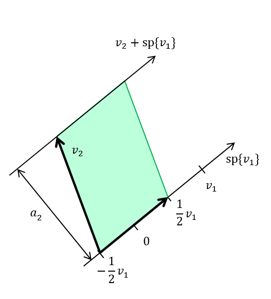
(a) $v_{1}$, $v_{2}$ and $a_{2}$ in the plane $\mbox{span}_{\mathbb{R}}\left\{v_{1},v_{2}\right\}=\mbox{span}_{\mathbb{R}}\left(\Lambda\right)$

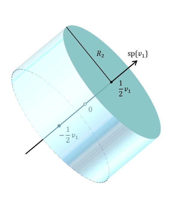
(b) A Dirichlet domain for $\tilde{\Lambda}_{1}$, $\left[-1/2,1/2\right]v_{1}$, multiplied by a ball of radius $R_{2}$.

Figure 4: Lemma 6.3.

Lemma 6.3.

Assume that $\Lambda_{\#}$ is a full lattice in $\mathbb{R}^{n}$ with covolume $\mathbf{v}$, and set $1\leq d\leq n$. Let there be $d-1$ intervals $\left[\alpha_{i},\beta_{i}\right]$ with $0\leq\alpha_{i}<\beta_{i}$. The number of rank $d$ subgroups of $\Lambda_{\#}$ whose covolume is $\leq X$ and who satisfy that $\operatorname{covol}(\Lambda^{i})\in[X^{\alpha_{i}},X^{\beta_{i}}]$ for some reduced basis $\{v_{1},\ldots,v_{d}\}$ such that $\Lambda^{i}:=\mbox{span}_{\mathbb{Z}}\{v_{1},\ldots,v_{i}\}$, is $O_{n}(\mathbf{v}^{-d}X^{e\left(\underline{\alpha},\underline{\beta}\right)})$, where

$$e(\underline{\alpha},\underline{\beta})=n-d+1+2\sum_{i=1}^{d-1}\beta_{i}+\sum_{i=1}^{d-1}(n-i)(\beta_{i}-\alpha_{i}).$$

Proof.

Let $\Lambda<\Lambda_{\#}$ be a rank $d$ subgroup, and write $\Lambda=\mbox{span}_{\mathbb{Z}}\left\{v_{1},\ldots,v_{n-1}\right\}$ where $\left\{v_{1},\ldots,v_{n-1}\right\}$ is a reduced basis for $\Lambda$. We use the notations introduced in Definition 3.5: $\left\{\phi_{1},\dots,\phi_{n-1}\right\}$ is the Gram-Schmidt basis obtained from $\left\{v_{1},\ldots,v_{n-1}\right\}$, $V_{i}$ is $\mbox{span}\left\{v_{1},\ldots,v_{i}\right\}=\mbox{span}\left\{\phi_{1},\dots,\phi_{i}\right\}$, and $a_{i}$ is the projection of $v_{i}$ on the line orthogonal to $V_{i-1}$ inside the space $V_{i}$, where $\mbox{span}\left\{\emptyset\right\}$ is set to be the trivial subspace $\left\{0\right\}$. In other words, $a_{i}$ is the distance of $v_{i}$ from the subspace $V_{i-1}$ (Figure 4a). If $\Lambda$ is such that $\operatorname{covol}(\Lambda^{i})\in\left[X^{\alpha_{i}},X^{\beta_{i}}\right]$, then $a_{i}\leq R_{i}=X^{\beta_{i}-\alpha_{i-1}}$. Denote the number of possibilities for choosing $v_{i}$ given that $\Lambda^{i-1}$ is known by $\#v_{i}|_{\Lambda^{i-1}}$. We first claim that for every $1\leq i\leq d$

$$\#v_{i}|_{\Lambda^{i-1}}=O\left((R_{i})^{n-i+1}\cdot\mathbf{v}^{-1}\cdot\operatorname{covol}(\Lambda^{i-1})\right).$$ (6.1)

Indeed, for $i=1$, the number $\#v_{i}|_{\Lambda^{i-1}}$ is simply the number of possibilities for choosing a $\Lambda_{\#}$ vector $v_{1}$ inside a ball of radius $a_{1}=\left\|v_{1}\right\|$ in $\mathbb{R}^{n}$, and therefore

$$\#v_{1}|_{\Lambda^{0}}=\#(\Lambda_{\#}\cap B_{R_{1}})=O(\mathbf{v}^{-1}\cdot R_{1}^{n}).$$

For $i>1$, the orthogonal projection of $v_{i}$ to the subspace $V_{i-1}$ must lie inside a Dirchlet domain of the lattice $\tilde{\Lambda}^{i-1}:=\mbox{span}_{\mathbb{Z}}\left\{a_{1}\phi_{1},\dots,a_{i-1}\phi_{i-1}\right\}$. Thus, $v_{i}$ has to be chosen from the set of $\Lambda_{\#}$ points which are of distance $\leq a_{i}\leq R_{i}$ from the Dirichlet domain for $\tilde{\Lambda}^{i-1}$ in $\mbox{span}_{\mathbb{R}}(\Lambda^{i-1})$. These are the $\Lambda_{\#}$ points that lie in a domain which is the product of the Dirichlet domain for $\tilde{\Lambda}^{i-1}$ (in $V_{i-1}$) with a ball of radius $R_{i}$ in the $n-\left(i-1\right)$ dimensional subspace $V_{i-1}^{\perp}$ (Figure 4b). Denote this ball by $B_{R_{i}}^{n-\left(i-1\right)}$, and then

$$\#v_{i}|_{\Lambda^{i-1}} \leq \#(\Lambda_{\#}\cap\{B_{R_{i}}^{n-\left(i-1\right)}\times\mbox{Dirichlet domain for $\tilde{\Lambda}^{i-1}$}\})$$

$$= O(\mathbf{v}^{-1}\cdot\operatorname{vol}(B_{R_{i}}^{n-\left(i-1\right)})\cdot\operatorname{covol}(\Lambda^{i-1}))$$

$$= O(\mathbf{v}^{-1}\cdot(R_{i})^{n-i+1}\cdot\operatorname{covol}(\Lambda^{i-1})).$$

This establishes Equation (6.1). Now, the number of possibilities for $\Lambda$ is given by:

$$\prod_{i=1}^{d}(\#v_{i}|_{\Lambda^{i-1}})=O(\prod_{i=1}^{d}(\mathbf{v}^{-1}\cdot(R_{i})^{n-i+1}\cdot\operatorname{covol}(\Lambda^{i-1})))$$

$$=O(\mathbf{v}^{-d}\prod_{i=1}^{d}(X^{\left(\beta_{i}-\alpha_{i-1}\right)\left(n-i+1\right)}\cdot X^{\beta_{i-1}}))$$

where $\alpha_{0}=0$ and $\beta_{d}=1$ (as $\operatorname{covol}(\Lambda^{1})=\left\|v_{1}\right\|\geq X^{0}$, and $\operatorname{covol}(\Lambda^{d})=\operatorname{covol}(\Lambda)\leq X^{1}$). Since

$$\sum_{i=1}^{d}((n-i+1)(\beta_{i}-\alpha_{i-1})+\beta_{i-1})=n-d+1+\sum_{i=1}^{d-1}(n-i)(\beta_{i}-\alpha_{i})+2\sum_{i=1}^{d-1}\beta_{i}=e(\underline{\alpha},\underline{\beta})$$

then the number of lattices $\Lambda$ is bounded by $O(\mathbf{v}^{-d}X^{e(\underline{\alpha},\underline{\beta})})$. ∎

Corollary 6.4.

Assume that $\Lambda_{\#}$ is a full lattice in $\mathbb{R}^{n}$ with covolume $\mathbf{v}$, let $1\leq d\leq n$, and $0<\omega_{1}<\cdots<\omega_{d-1}$. For every $\epsilon>0$, the number of rank $d$ subgroups of $\Lambda_{\#}$ with covolume $\leq X$ which satisfy $\operatorname{covol}(\Lambda^{i})\in[1,X^{\omega_{i}}]$ is $O_{\epsilon}\,(\mathbf{v}^{-d}\cdot X^{n-d+1+2\omega+\epsilon})$, where $\omega:=\sum_{i=1}^{d-1}\omega_{i}$.

Proof.

Divide every interval $[0,\omega_{i}]$ into $N_{i}=N_{i}(\omega_{i})$ sub-intervals

$$0=\beta_{0}^{i}<\beta_{1}^{i}<\ldots<\beta_{N_{i}}^{i}=\omega_{i}$$

such that $|\beta_{j}^{i}-\beta_{j-1}^{i}|\leq\epsilon$ for every $j=1,\ldots,N_{i}$. By refining these partitions, we may assume without loss of generality that $N_{1}=\ldots=N_{d-1}:=N$. Fix $j\in\left\{1,\ldots,N\right\}$; according to Lemma 6.3, the number of rank $d$ subgroups $\Lambda$ of $\Lambda_{\#}$ with $\operatorname{covol}(\Lambda)\leq X$ and $\operatorname{covol}(\Lambda^{i})\in[X^{\beta_{j-1}^{i}},X^{\beta_{j}^{i}}]$ for every $i=1\ldots d-1$ is of order $X$ to the power of

$$n-d+1+2\sum_{i=1}^{d-1}\beta_{j}^{i}+\sum_{i=1}^{d-1}\left(n-i\right)(\beta_{j}^{i}-\beta_{j-1}^{i}) \leq n-d+1+2\sum_{i=1}^{d-1}\omega_{i}+\sum_{i=1}^{d-1}\left(n-i\right)\cdot\epsilon$$

$$= n-d+1+2\omega+\epsilon\cdot\left(d-1\right)\left(n-d/2\right),$$

where we have used $|\beta_{j}^{i}-\beta_{j-1}^{i}|\leq\epsilon$ and $\beta_{j}^{i}\leq\omega_{i}$.

Let $\Lambda<\Lambda_{\#}$ be as in the statement. Since $\operatorname{covol}(\Lambda^{i})$ lies in $[X^{0},X^{\omega_{i}}]$ for every $i=1,\ldots,d-1$, then for every $i$ there exist $j_{1}^{i},\ldots j_{d-1}^{i}$ such that $\operatorname{covol}(\Lambda_{i})\in[X^{\beta_{j-1}^{i}},X^{\beta_{j}^{i}}]$. It follows that

$$\#\Lambda=O_{\epsilon}(\mathbf{v}^{-d}\sum_{\begin{subarray}{c}\left\{j_{1},\ldots j_{n-2}\right\}\\ \subset\left\{1,\ldots,N\right\}\end{subarray}}X^{n-d+1+2\omega+\epsilon\cdot O_{n}\left(1\right)})=O_{\epsilon}(\mathbf{v}^{-d}X^{n-d+1+2\omega+\epsilon}).$$

Proof of Proposition 6.2.

Let $\gamma_{v}=ka_{\underline{s}}^{\prime\prime}a_{t}^{\prime}n\in\gamma\in\Omega_{T}\cap\operatorname{SL}_{n}\left(\mathbb{Z}\right)$. By definition of $\Omega_{T}^{\left[\underline{\sigma}T;\infty\right]}$ we have that $\gamma\in\Omega_{T}^{\left[\underline{\sigma}T;\infty\right]}$ if and only if $t\in\left[0,T\right]$ and $s_{i}\geq\sigma_{i}T$ for some $i$. According to Proposition 2.2, (by which $\operatorname{covol}(\Lambda_{v}^{i})=e^{\frac{it}{n-1}-\frac{s_{i}}{2}}$), and since $\Lambda_{v}^{i}$ is integral, we have that $1\leq\operatorname{covol}(\Lambda_{v}^{i})\leq e^{(\frac{i}{n-1}-\frac{\sigma_{i}}{2})T}$. Thus, the number of $\operatorname{SL}_{n}\left(\mathbb{Z}\right)$-elements $\gamma$ in $\Omega_{T}^{\left[\underline{\sigma}T;\infty\right]}$ is bounded by the number of $\left(n-1\right)$-dimensional subgroups $\Lambda_{v}$ of $\mathbb{Z}^{n}$ of co-volume $\leq e^{T}:=X$, for which there exists $i\in\left\{1,\ldots,n-2\right\}$ such that $\operatorname{covol}(\Lambda_{v}^{i})\in[1,X^{\frac{i}{n-1}-\frac{\sigma_{i}}{2}}]$, where for $j\neq i$ $\operatorname{covol}(\Lambda_{v}^{j})\in[1,X^{\frac{j}{n-1}}]$. In other words,

$$\#(\Omega_{T}^{\left[\underline{\sigma}T;\infty\right]}\cap\operatorname{SL}_{n}\left(\mathbb{Z}\right))=\#(\bigcup_{\begin{subarray}{c}\underline{u}=(u_{1},\ldots,u_{n-2})\\ \in\left\{0,1\right\}^{n-2}-\left\{0\right\}\end{subarray}}\{\Lambda_{v}:\forall i,\,\operatorname{covol}(\Lambda_{v}^{i})\in[1,X^{\frac{i}{n-1}-\frac{\sigma_{i}u_{i}}{2}}]\})$$

which by Corollary 6.4 with $e^{T}=X$, $d=n-1$ and $\frac{i}{n-1}-\frac{\sigma_{i}u_{i}}{2}=\omega_{i}$ equals to

$$\sum_{\underline{u}\in\left\{0,1\right\}^{n-2}-\left\{0\right\}}O_{\epsilon}(X^{2+n-2+\epsilon-\sum_{i=1}^{n-2}\sigma_{i}u_{i}})=O_{\epsilon}(X^{n-\sigma_{\min}+\epsilon})$$

where $\sigma_{\min}=\min\left\{\sigma_{i}\right\}$. ∎

7 Almost a proof for Theorems A and B

In Section 5 (see Corollary 5.3), the proof of Theorem B was reduced to counting integral matrices in three families of subsets of $\Omega_{\operatorname{short}}\subset\operatorname{SL}_{n}\left(\mathbb{R}\right)$. But, as we shall see, it is in fact sufficient to count integral matrices in only one of these families, the one corresponding to part 3 of Theorem B: $\left(\Omega_{\operatorname{short}}\right)_{T}(\Psi,\alpha)$. The content of this section is a proof of Theorem B, assuming the following (yet to be proved) counting statement in this family:

Proposition 7.1.

For $\alpha\in\left(0,1\right)$, assume that $\Psi\subseteq\mathcal{L}_{n-1,n}$ is BCS. Set $\lambda_{n}=n^{2}/\left(2\left(n^{2}-1\right)\right)$, and let $\tau_{n}$ be as in Theorem B.

1. For $\epsilon\in(0,\tau_{n})$, $\underline{S}=(S_{1},\dots,S_{n-2})$, $\mathbf{S}=\sum_{i=1}^{n-2}S_{i}$ and every $T\geq\frac{\mathbf{S}}{n\lambda_{n}\tau_{n}}+O\left(1\right)$,

   $$\#((\Omega_{\operatorname{short}})_{T}^{\underline{S}}(\Psi,\alpha)\cap\operatorname{SL}_{n}\left(\mathbb{Z}\right))=\frac{\mu((\Omega_{\operatorname{short}})_{T}^{\underline{S}}(\Psi,\alpha))}{\mu\left(\operatorname{SL}_{n}\left(\mathbb{R}\right)/\operatorname{SL}_{n}\left(\mathbb{Z}\right)\right)}+O_{\epsilon,\Psi}(e^{\mathbf{S}/\lambda_{n}}e^{nT\left(1-\tau_{n}+\epsilon\right)}).$$

2. For $\epsilon>0$, $\delta\in\left[0,\tau_{n}-\epsilon\right)$, $T\geq O\left(1\right)$ and $\underline{S}\left(T\right)$ such that $\sum S_{i}\left(T\right)\leq n\delta\lambda_{n}T+O_{\Psi}(1)$,

   $$\#((\Omega_{\operatorname{short}})_{T}^{\underline{S}\left(T\right)}(\Psi,\alpha)\cap\operatorname{SL}_{n}\left(\mathbb{Z}\right))=\frac{\mu((\Omega_{\operatorname{short}})_{T}^{\underline{S}\left(T\right)}(\Psi,\alpha))}{\mu\left(\operatorname{SL}_{n}\left(\mathbb{R}\right)/\operatorname{SL}_{n}\left(\mathbb{Z}\right)\right)}+O_{\epsilon,\Psi}(e^{nT\left(1-\tau_{n}+\delta+\epsilon\right)}).$$

Notice that the difference between parts 1 and 2 of the proposition above is that in the first part $\underline{S}$ is fixed, while in the second part, at the cost of compromising the error term, we allow the sum of $S_{i}$-s to grow proportionally to $T$.

Remark 7.2.

If $\Psi\subset\mathcal{L}_{n-1,n}$ is also bounded, then for suitable $\underline{S}$ one has that $(\Omega_{\operatorname{short}})_{T}^{\underline{S}}(\Psi,\alpha)=(\Omega_{\operatorname{short}})_{T}(\Psi,\alpha)$; thus in this case part 1 of Proposition 7.1 can be written as

$$\#\left((\Omega_{\operatorname{short}})_{T}\cap\operatorname{SL}_{n}\left(\mathbb{Z}\right)\right)=\mu\left((\Omega_{\operatorname{short}})_{T}\right)/\mu\left(\operatorname{SL}_{n}\left(\mathbb{R}\right)/\operatorname{SL}_{n}\left(\mathbb{Z}\right)\right)+O_{\epsilon}(e^{nT\left(1-\tau_{n}+\epsilon\right)}),$$

where the implied constant depends on $\Psi$.

The proof of Proposition 7.1 is in Section 13. Let us now prove Theorem B based on this proposition:

Proof of Theorem B.

According to Corollary 5.3 and to Lemma 4.5, the quantities we seek to estimate in parts (1), (2) and (3) of the theorem is in one to one correspondence with the integral matrices in the following subsets of $\operatorname{SL}_{n}\left(\mathbb{R}\right)$: (1) $(\Omega_{\operatorname{short}})_{T}(\Phi,\mathcal{E},\alpha)$, (2) $(\Omega_{\operatorname{short}})_{T}(\Phi,\widetilde{\mathcal{E}},\alpha)$, or (3) $(\Omega_{\operatorname{short}})_{T}(\Psi,\alpha)$. Observe that, indeed the main terms in the theorem are the volumes of these sets, divided by the measure of $\operatorname{SL}_{n}\left(\mathbb{R}\right)/\operatorname{SL}_{n}\left(\mathbb{Z}\right)$. Let us demonstrate the computation for the case of the family (1), for which we recall the notation for the fibers $K_{z_{i}}^{\prime\prime}$ and the generic fiber $K_{\text{gen}}^{\prime\prime}$ appearing in the proof of Lemma 3.9:

$$\mu\left(\left(\Omega_{\operatorname{short}}\right)_{T}(\Phi,\mathcal{E},\alpha)\right)=\mu\left(\bigcup_{p^{\prime\prime}\in P^{\prime\prime}_{\mathcal{E}}}K^{\prime}_{\Phi}\cdot K_{z^{p^{\prime\prime}}}^{\prime\prime}\cdot p^{\prime\prime}\cdot A_{T}^{\prime}N^{\prime}_{Y^{\alpha}(z^{p^{\prime\prime}})}\right)=$$

$$=\mu_{K^{\prime}}\left(K_{\Phi}^{\prime}\right)\mu_{K^{\prime\prime}}\left(K_{\text{gen}}^{\prime\prime}\right)\mu_{A^{\prime}}\left(A_{T}^{\prime}\right)\int_{P^{\prime\prime}_{\mathcal{E}}\cap\operatorname{int}\left(F_{n-1}\right)}\mu_{N^{\prime}}\left(N^{\prime}_{Y^{\alpha}(z^{p^{\prime\prime}})}\right)d\mu_{P^{\prime\prime}}\left(p^{\prime\prime}\right)$$

$$+\sum_{i}\mu_{K}\left(K_{\Phi}^{\prime}K_{z_{i}}^{\prime\prime}\right)\mu_{A^{\prime}}\left(A_{T}^{\prime}\right)\int_{\begin{subarray}{c}P^{\prime\prime}_{\mathcal{E}}\cap\partial F_{n-1}\cap\\ \left\{p^{\prime\prime}:\mbox{Sym}^{+}\left(\Lambda_{p^{\prime\prime}}\right)=\mbox{Sym}^{+}\left(\Lambda_{z_{i}}\right)\right\}\end{subarray}}\mu_{N^{\prime}}\left(N^{\prime}_{Y^{\alpha}(z^{p^{\prime\prime}})}\right)d\mu_{P^{\prime\prime}}\left(p^{\prime\prime}\right),$$

where we have used: the definition 5.1 for $\left(\Omega_{\operatorname{short}}\right)_{T}(\Phi,\mathcal{E},\alpha)$, Formula 2.7 for the decomposition of $\mu$ to RI components and Proposition 3.8 which tells us that all the interior points in $F_{n-1}$ have the generic fiber. Now, the second summand is of measure zero, since the boundary of $F_{n-1}$ is such, so we are left only with the first summand.

Since, by “Measures on the RI components” in Section 2, $\mu_{N^{\prime}}$ is the Lebesgue measure on $\mathbb{R}^{n-1}$, $\mu_{K^{\prime}}$ is the Lebesgue measure on $\mathbb{S}^{n-1}$, the volume of $\operatorname{SO}_{n-1}\left(\mathbb{R}\right)$ is $\prod_{i=1}^{n-2}\operatorname{Leb}(\mathbb{S}^{i})$ (implying that the measure of $K_{\text{gen}}^{\prime\prime}$ is $\prod_{i=1}^{n-2}\operatorname{Leb}(\mathbb{S}^{i})/\iota\left(n-1\right)$), and the $\mu_{A^{\prime}}\left(A_{T}^{\prime}\right)=e^{nT}/n$, and since by Proposition 3.2 we can pass from integration on $F_{n-1}$ to integration on $\mathcal{X}_{n-1}$, we have that the above equals to

$$\frac{e^{nT}\cdot\mu_{\mathbb{S}^{n-1}}\left(\Phi\right)\cdot\prod_{i=1}^{n-2}\operatorname{Leb}(\mathbb{S}^{i})}{n\cdot\iota\left(n-1\right)}\int_{\mathcal{E}}\text{L}_{\alpha}(z)d\mu_{\mathcal{X}_{n-1}}\left(z\right),$$

as wanted.

We claim that it is sufficient to prove part (3) of the theorem, since parts (1) and (2) are special cases. Indeed, family (1) is a special case of family (2), when taking $\widetilde{\mathcal{E}}\subseteq\mathcal{U}_{n-1}$ to be the inverse image of $\mathcal{E}\subseteq\mathcal{U}_{n-1}$. This is because Lemma 3.9 gives that the lift $\widetilde{\mathcal{E}}$ is a BCS when $\mathcal{E}$ is, so the assumption of part 1 of the theorem implies the assumption in part 2 for the lifts; moreover, this Lemma gives that $\text{$\mu_{\mathcal{U}_{n-1}}(\widetilde{\mathcal{E}})$}=\mu_{\mathcal{X}_{n-1}}(\mathcal{E}){\scriptstyle\prod}_{i=1}^{n-2}\operatorname{Leb}(\mathbb{S}^{i})/\iota\left(n-1\right)$, so the main term provided in part 2 for $\widetilde{\mathcal{E}}$ and $\Phi$ coincides with the one provided in part 1 of this theorem for $\mathcal{E}$ and $\Phi$. Similarly, family (2) is a special case of family (3), when taking $\Psi$ such that $Q_{\Psi}=K^{\prime}_{\Phi}G^{\prime\prime}_{\widetilde{\mathcal{E}}}$. By Lemma 3.9, $\Psi$ is a BCS when $\widetilde{\mathcal{E}}$ and $\Phi$ are, and $\mu_{\mathcal{L}_{n,n-1}}(\Psi)=\mu_{\mathcal{U}_{n-1}}(\widetilde{\mathcal{E}})\mu_{\mathbb{S}^{n-1}}(\Phi)$. We therefore prove only part 3 of Theorem B.

(i) Let us first consider the case where $\Psi$ is not bounded, and therefore $(\Omega_{\operatorname{short}})_{T}(\Psi,\alpha)$ is not bounded also. Fix $\epsilon\in(0,\tau_{n})$, $\delta\in(0,\tau_{n}-\epsilon)$, and $\underline{\sigma}_{n}:=(\frac{\delta n\lambda_{n}}{n-2}-\epsilon)\cdot\underline{1}$, where $\lambda_{n}=\frac{n^{2}}{2\left(n^{2}-1\right)}$; note that the sum of the coordinates of $\underline{\sigma}_{n}$ is $\delta n\lambda_{n}-\left(n-2\right)\epsilon$, which is smaller than $\delta n\lambda_{n}+O_{\Psi}(1)/T$ for $T$ large enough. Using Proposition 6.2, we reduce to counting in compact sets $(\Omega_{\operatorname{short}})_{T}^{\underline{\sigma}_{n}T}(\Psi,\alpha)$, and pay with an error term of $O_{\epsilon}(e^{nT(1-\frac{\delta\lambda_{n}}{n-2}+\frac{\epsilon}{n}+\epsilon)})$, which we can write as $O_{\epsilon}(e^{nT(1-\frac{\delta\lambda_{n}}{n-2}+\epsilon)})$ since $\epsilon$ is arbitrary. (ii) Counting integral matrices in the sets $(\Omega_{\operatorname{short}})_{T}^{\underline{\sigma}_{n}T}(\Psi,\alpha)$ will complete the proof, and it is performed using (the second part of) Proposition 7.1, based on which it equals

$$\mu(\,(\Omega_{\operatorname{short}})_{T}^{\underline{\sigma}_{n}T}(\Psi,\alpha))+O_{\epsilon}(e^{nT\left(1-\tau_{n}+\delta+\epsilon\right)}).$$

Since $\mu\left((\Omega_{\operatorname{short}})_{T}(\Psi,\alpha)\right)=\mu((\Omega_{\operatorname{short}})_{T}^{\underline{\sigma}_{n}T}(\Psi,\alpha))+O(e^{nT(1-\frac{\delta\lambda_{n}}{n-2})})$ (see remark about the measure in Notation 6.1), and the error term is swallowed in the one obtained in step (i), we obtain

$$\#\left((\Omega_{\operatorname{short}})_{T}(\Psi,\alpha)\cap\operatorname{SL}_{n}\left(\mathbb{Z}\right)\right)=\mu\left((\Omega_{\operatorname{short}})_{T}(\Psi,\alpha)\right)+O_{\epsilon}(e^{nT\left(1-\tau_{n}+\delta+\epsilon\right)})+O_{\epsilon}(e^{nT(1-\frac{\delta\lambda_{n}}{n-2}+\epsilon)}).$$

(iii) We now choose $\delta$ that will balance the two error terms above: $1-\tau_{n}+\delta=1-\frac{\delta\lambda_{n}}{n-2}$ if and only if $\delta=\tau_{n}/(1+\frac{\lambda_{n}}{n-2})=\tau_{n}\cdot\left(1-\frac{n^{2}}{2n^{3}-3n^{2}-2n+4}\right)$ . Then the final error term for non bounded $\Psi$ is $e^{nT\left(1-\tau_{n}\cdot\frac{n^{2}}{2n^{3}-3n^{2}-2n+4}\right)}$. (iv) Moving forward to bounded $\Psi$, we repeat a similar strategy as in the unbounded case, performing only step (ii). Fix $\epsilon\in\left(0,\tau_{n}\right)$ and apply Proposition 7.1 (case of Remark 7.2) to obtain that the number of integral matrices in $(\Omega_{\operatorname{short}})_{T}(\Psi,\alpha)$ is $\mu\left((\Omega_{\operatorname{short}})_{T}(\Psi,\alpha)\right)+O_{\epsilon}\left(e^{nT\left(1-\tau+\epsilon\right)}\right)$. This completes the proof for the bounded case in the theorem. ∎

Proof of Theorem A.

Let

$$\mathcal{B}=\,\Omega_{\operatorname{short}}\,\cap\,\left\{g=ka_{\underline{s}}^{\prime\prime}a_{t}^{\prime}n^{\prime}:s_{n-2}\in[0,t/2]\right\}.$$

We define

$$\mathcal{A}=\{v\in\mathbb{Z}_{\operatorname{prim}}^{n}:\gamma_{v}\in\mathcal{B}\},$$

and claim that it is a set of full density in $\mathbb{Z}_{\operatorname{prim}}^{n}$. In fact, we show that $\mathbb{Z}_{\operatorname{prim}}^{n}-\mathcal{A}$ is a set of density zero. For this, we note that the set $\Omega_{\operatorname{short}}-\mathcal{B}$ is contained in the set

$$\widetilde{\mathcal{B}}=\lim_{T\to\infty}\widetilde{\mathcal{B}}_{T}$$

where

$$\widetilde{\mathcal{B}}_{T} =\coprod_{t=1}^{T}(\left(\Omega_{\operatorname{short}}\right)_{t}-\left(\Omega_{\operatorname{short}}\right)_{t-1})\cap\left\{g=ka^{\prime}a_{\underline{s}}^{\prime\prime}n:\begin{matrix}0\leq s_{1},\ldots,s_{n-3},\\ \frac{1}{2}(t-1)\leq s_{n-2}\end{matrix}\right\}.$$

Note that $\widetilde{\mathcal{B}}_{T}$ can also be written as the disjoint union

$$\widetilde{\mathcal{B}}_{T}=\coprod_{t=1}^{T}(\left(\Omega_{\operatorname{short}}\right)_{t}-\left(\Omega_{\operatorname{short}}\right)_{t}^{(0,\ldots,0,\frac{1}{2}(t-1))})-(\left(\Omega_{\operatorname{short}}\right)_{t-1}-\left(\Omega_{\operatorname{short}}\right)_{t-1}^{(0,\ldots,0,\frac{1}{2}(t-1))}).$$ (7.1)

As a result, the volume of $\widetilde{\mathcal{B}}_{T}$ can be bounded as follows:

$$\mu\left(\widetilde{\mathcal{B}}_{T}\right) \leq\sum_{t=1}^{T}\mu(\left(\Omega_{\operatorname{short}}\right)_{t}-\left(\Omega_{\operatorname{short}}\right)_{t}^{(0,\ldots,0,\frac{1}{2}(t-1))})$$

$$\ll\sum_{t=1}^{T}\left(\int_{\frac{1}{2}(t-1)}^{\infty}e^{-s_{n-2}}ds_{n-2}\right)\int_{t-1}^{t}e^{n\tau}d\tau$$

$$=\frac{1}{n}\sum_{t=1}^{T}e^{-\frac{1}{2}t+\frac{1}{2}}(e^{nt}-e^{n(t-1)})$$

$$\leq Te^{(n-\frac{1}{2})T}.$$

The presentation in (7.1) can also be used to estimate the number of $\operatorname{SL}_{n}\left(\mathbb{Z}\right)$ elements in $\widetilde{\mathcal{B}}_{T}$, by counting $\operatorname{SL}_{n}\left(\mathbb{Z}\right)$ elements in each of the summands separately. For this, Let $\delta$ and $\underline{\sigma}_{n}=(\sigma_{1},\ldots,\sigma_{n-2})$ be as in the proof of the unbounded case in Theorem B. Going along the lines of this proof, we can reduce counting in each (non-compact) summand to counting in the truncated set

$$(\Omega_{\operatorname{short}})_{t}^{\underline{\sigma}_{n}t}-(\Omega_{\operatorname{short}})_{t}^{(\sigma_{1}t,\ldots,\sigma_{n-3}t,\min\{\sigma_{n-2}t,\frac{1}{2}(t-1)\})}$$

$$\left.\right.\hfill\left.\right.\hfill-\left((\Omega_{\operatorname{short}})_{t-1}^{\underline{\sigma}_{n}t}-(\Omega_{\operatorname{short}})_{t-1}^{(\sigma_{1}t,\ldots,\sigma_{n-3}t,\min\{\sigma_{n-2}t,\frac{1}{2}(t-1)\})}\right),$$

since according to Proposition 6.2, the difference in the amount of lattice points inside each summand and its truncation lies in $O_{\epsilon}(e^{nt(1-\frac{\delta\lambda_{n}}{n-2}+\epsilon)})$, and the difference between their measures is also swallowed in this error estimate (see remark about the measure in Notation 6.1). Using Proposition 7.1(ii) to estimate the amount of lattice points in each truncated summand, we obtain that the number of lattice points in each (full) summand is its measure divided by $\mu(\operatorname{SL}_{n}(\mathbb{R})/\operatorname{SL}_{n}(\mathbb{Z}))$, up to an error term of order $O_{\epsilon}(e^{nt(1-\frac{\delta\lambda_{n}}{n-2}+\epsilon)})$. As a result,

$$\#(\widetilde{\mathcal{B}}_{T}\cap\operatorname{SL}_{n}(\mathbb{Z}))=\frac{\mu(\widetilde{\mathcal{B}}_{T})}{\mu(\operatorname{SL}_{n}(\mathbb{R})/\operatorname{SL}_{n}(\mathbb{Z}))}+O_{\epsilon}(Te^{nT(1-\frac{\delta\lambda_{n}}{n-2}+\epsilon)}).$$

According to Corollary 5.3,

$$\lim_{T\to\infty}\frac{\#((\mathbb{Z}_{\operatorname{prim}}^{n}-\mathcal{A})\cap B_{e^{T}})}{\#(\mathbb{Z}_{\operatorname{prim}}^{n}\cap B_{e^{T}})}=\lim_{T\to\infty}\frac{\#(((\Omega_{\operatorname{short}})_{T}-\mathcal{B})\cap\operatorname{SL}_{n}(\mathbb{Z}))}{\#((\Omega_{\operatorname{short}})_{T}\cap\operatorname{SL}_{n}(\mathbb{Z}))}$$

which by definition of $\widetilde{\mathcal{B}}$ is at most

$$\leq\lim_{T\to\infty}\frac{\#(\widetilde{\mathcal{B}}_{T}\cap\operatorname{SL}_{n}(\mathbb{Z}))}{\#((\Omega_{\operatorname{short}})_{T}\cap\operatorname{SL}_{n}(\mathbb{Z}))}.$$

The denominator in the above limit is, according to Proposition 4.1 and Theorem B , asymptotic to

$$\frac{\mu((\Omega_{\operatorname{short}})_{T})}{\mu(\operatorname{SL}_{n}(\mathbb{R})/\operatorname{SL}_{n}(\mathbb{Z}))}\asymp e^{nT}.$$

We then have that

$$\lim_{T\to\infty}\frac{\#((\mathbb{Z}_{\operatorname{prim}}^{n}-\mathcal{A})\cap B_{e^{T}})}{\#(\mathbb{Z}_{\operatorname{prim}}^{n}\cap B_{e^{T}})}\leq\lim_{T\to\infty}\frac{\mu(\widetilde{\mathcal{B}}_{T})}{\mu((\Omega_{\operatorname{short}})_{T})}=\lim_{T\to\infty}\frac{Te^{(n-\frac{1}{2})T}}{e^{nT}}=0,$$

which establishes that $\mathcal{A}$ is a set of full density in $\mathbb{Z}_{\operatorname{prim}}^{n}$.

For a primitive vector $v$ with large enough norm, we have by Lemma 4.5 and definition of $w_{v}$ that

$$0<\frac{\left\|w_{v}\right\|}{\left\|v\right\|}\ll\frac{\left\|w_{v}^{\perp}\right\|}{\left\|v\right\|}\leq\frac{\rho_{v}}{\left\|v\right\|}=\frac{\rho_{v}}{\operatorname{covol}(\Lambda_{v})}.$$

Minkowski’s 2nd Theorem gives us that $\rho_{v}=\rho(\Lambda_{v})\asymp\mathfrak{m}_{n-1}(\Lambda_{v})$, where $\mathfrak{m}_{i}$ denotes the $i$th successive minima. From [GM02, Theorem 7.9] we have that $\operatorname{covol}(\Lambda_{v})\asymp\mathfrak{m}_{1}(\Lambda_{v})\cdots\mathfrak{m}_{n-1}(\Lambda_{v})$. Thus the above can be further estimated as:

$$\ll\frac{\mathfrak{m}_{n-1}(\Lambda_{v})}{\mathfrak{m}_{1}(\Lambda_{v})\cdots\mathfrak{m}_{n-1}(\Lambda_{v})}=\frac{1}{\mathfrak{m}_{1}(\Lambda_{v})\cdots\mathfrak{m}_{n-2}(\Lambda_{v})}\ll\operatorname{covol}(\Lambda_{v}^{n-2})^{-1},$$

where by Proposition 2.2(iii),

$$\ll e^{\frac{s_{n-2}}{2}-\frac{n-2}{n-1}t}\leq e^{-\frac{3n-6}{4(n-1)}t}.$$

The above decays to $0$ if (and only if) $n>2$, and we are done – since if $\{v_{m}\}\subset\mathcal{A}$ diverges, then $\gamma_{v_{m}}=k_{m}a_{m}^{\prime\prime}a_{t_{m}}^{\prime}n_{m}$ with $t_{m}\to\infty$ as $m\to\infty$, implying that $\left\|w_{v_{m}}\right\|/\left\|v_{m}\right\|\to 0$. ∎

Part II Counting lattice points

This second part is the technical part of the paper, where we prove Proposition 7.1, in order to conclude the proof of Theorem B. This proposition concerns counting lattice points in $\operatorname{SL}_{n}\left(\mathbb{R}\right)$; our main tool for this purpose is a method introduced in [GN12] for counting lattice points in increasing families of sets inside semisimple Lie groups. The advantages of this method is that it produces an error term, and that it allows counting in quite general families, requiring only that these families are well rounded, which is a regularity condition. The cost of this generality is that the property of well roundedness is often hard to verify. In [HK20] we develop a machinery to somewhat simplify this process, mainly by allowing us to replace the underlying simple group $G=KAN$ with the much-easier-to-work-in Cartesian product $K\times A\times N$; we will refer to some technical results from there in the course of Part II.

8 Counting lattice points in well rounded families of sets inside Lie groups

We begin in Subsection 8.1 by describing the counting lattice points method that we will use, and proceed in Subsection 8.2 with laying out a plan of proof for Proposition 7.1. From now on, we use $\Gamma$ to denote a general lattice in a Lie group, hence abandoning the notation in Section 4.

8.1 A method for lattice points counting in Well rounded families

In this subsection we briefly describe the counting method developed in [GN12]. This approach, aimed at counting lattice points in increasing families of sets inside non-compact algebraic simple Lie groups, consists of two ingredients: a regularity condition on the sets involved, and a spectral estimate concerning the unitary $G$ representation $\pi_{G/\Gamma}^{0}:G\to L_{0}^{2}\left(G/\Gamma\right)$ (the orthogonal complement of the $G$ invariant $L^{2}$ functions). Before stating the counting theorem 8.4 from [GN12], we describe the two ingredients, starting with the regularity condition.

Definition 8.1.

Let $G$ be a Lie group with a Borel measure $\mu$, and let $\{\mathcal{O}_{\epsilon}\}_{\epsilon>0}$ be a family of identity neighborhoods in $G$. Assume $\left\{\mathcal{B}_{T}\right\}_{T>0}\subset G$ is a family of measurable domains and denote

$$\mathcal{B}_{T}^{\left(+\epsilon\right)}:=\mathcal{O}_{\epsilon}\mathcal{B}_{T}\mathcal{O}_{\epsilon}=\bigcup_{u,v\in\mathcal{O}_{\epsilon}}u\,\mathcal{B}_{T}\,v,$$

$$\mathcal{B}_{T}^{\left(-\epsilon\right)}:=\bigcap_{u,v\in\mathcal{O}_{\epsilon}}u\,\mathcal{B}_{T}\,v$$

(see Figure 5). The family $\left\{\mathcal{B}_{T}\right\}$ is Lipschitz well rounded (LWR) with (positive) parameters $(\mathcal{C},T_{0})$ if for every $0<\epsilon<1/\mathcal{C}$ and $T>T_{0}$:

$$\mu\left(\mathcal{B}_{T}^{\left(+\epsilon\right)}\right)\leq\left(1+\mathcal{C}\epsilon\right)\>\mu\left(\mathcal{B}_{T}^{\left(-\epsilon\right)}\right).$$ (8.1)

The parameter $\mathcal{C}$ is called the Lipschitz constant of the family $\left\{\mathcal{B}_{T}\right\}$.

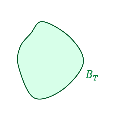
(a) The set $\mathcal{B}_{T}$

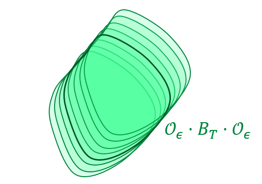
(b) The set $\mathcal{B}_{T}$ is perturbed by ${\cal O}_{\epsilon}$

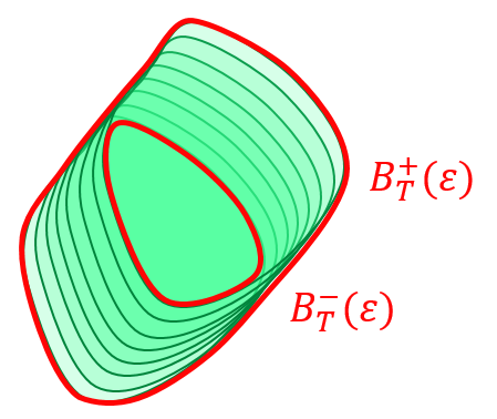
(c) $\mathcal{B}_{T}^{\left(-\epsilon\right)}$ and $\mathcal{B}_{T}^{\left(+\epsilon\right)}$

Figure 5: Well roundedness.

The definition above allows any family $\left\{\mathcal{O}_{\epsilon}\right\}_{\epsilon>0}$ of identity neighborhoods; in this paper we shall restrict to the following:

Assumption 8.2.

We will assume that $\mathcal{O}_{\epsilon}^{G}=\exp\left(B_{\epsilon}\right)$, where $B_{\epsilon}$ is an origin-centered $\epsilon$-ball inside the Lie algebra of $G$, and $\exp$ is the Lie exponent.

Remark 8.3.

We allow the case of a constant family $\left\{\mathcal{B}_{T}\right\}=\mathcal{B}$: we say that $\mathcal{B}$ is a Lipschitz well rounded set (as apposed to a Lipschitz well rounded family) with parameters $(\mathcal{C},\epsilon_{0})$ if $\mu(\mathcal{B}^{\left(+\epsilon\right)})\leq(1+\mathcal{C}\epsilon)\>\mu(\mathcal{B}^{\left(-\epsilon\right)})$ for every $0<\epsilon<\epsilon_{0}$. It is proved in [HK20, Prop. 3.5] that if a set $\mathcal{B}$ is BCS and bounded, then it is LWR.

We now turn to describe the second ingredient, which is the spectral estimation. In certain Lie groups, among which algebraic simple Lie groups $G$, there exists $p\in\mathbb{N}$ for which the matrix coefficients $\langle\pi_{G/\Gamma}^{0}u,v\rangle$ are in $L^{p+\epsilon}\left(G\right)$ for every $\epsilon>0$, with $u,v$ lying in a dense subspace of $L_{0}^{2}\left(G/\Gamma\right)$ (see [GN09, Thm 5.6]). Let $p\left(\Gamma\right)$ be the smallest among these $p$’s, and denote

$$m\left(\Gamma\right)=\begin{cases}1&\text{if $p=2$,}\\ 2\left\lceil p\left(\Gamma\right)/4\right\rceil&\text{otherwise.}\end{cases}$$

The parameter $m\left(\Gamma\right)$ appears in the error term exponent of the counting theorem below, which is the cornerstone of the counting results in this paper.

Theorem 8.4 ([GN12, Theorems 1.9, 4.5, and Remark 1.10]).

Let $G$ be an algebraic simple Lie group with Haar measure $\mu$, and let $\Gamma<G$ be a lattice. Assume that $\{\mathcal{B}_{T}\}\subset G$ is a family of finite-measure domains which satisfy $\mu(\mathcal{B}_{T})\to\infty$ as $T\to\infty$. If the family $\{\mathcal{B}_{T}\}$ is Lipschitz well rounded with parameters $(C_{\mathcal{B}},T_{0})$, then $\exists T_{1}>0$ such that for every $\delta>0$ and $T>T_{1}$:

$$\#(\mathcal{B}_{T}\cap\Gamma)-\mu(\mathcal{B}_{T})/\mu\left(G/\Gamma\right)\underset{G,\Gamma,\delta}{\ll}C_{\mathcal{B}}^{\frac{\dim G}{1+\dim G}}\cdot\mu(\mathcal{B}_{T})^{1-\tau\left(\Gamma\right)+\delta},$$

where $\mu\left(G/\Gamma\right)$ is the measure of a fundamental domain of $\Gamma$ in $G$ and

$$1-\tau\left(\Gamma\right)=1-(2m\left(\Gamma\right)\left(1+\dim G\right))^{-1}\in\left(0,1\right).$$

The parameter $T_{1}$ is such that $T_{1}\geq T_{0}$ and for every $T\geq T_{1}$

$$\mu\left(\mathcal{B}_{T}\right)^{\tau\left(\Gamma\right)}\underset{G,\Gamma}{\gg}C_{\mathcal{B}}^{\frac{\dim G}{1+\dim G}}.$$ (8.2)

Bounds on the parameter $p\left(\Gamma\right)$ (i.e. on $m\left(\Gamma\right)$) clearly imply bounds on the parameter $\tau\left(\Gamma\right)$ appearing in the error term exponent. We refer to [Li95], [LZ96] and [Sca90] for upper bounds on $p\left(\Gamma\right)$ in simple Lie groups. Specifically for the group $\operatorname{SL}_{n}\left(\mathbb{R}\right)$, the current known bound for $n>2$ and any lattice $\Gamma$ in $\operatorname{SL}_{n}\left(\mathbb{R}\right)$ is $2\leq p\left(\Gamma\right)\leq 2n-2$ [Li95]. For the lattice $\Gamma=\operatorname{SL}_{n}\left(\mathbb{Z}\right)$, $p\left(\operatorname{SL}_{n}\left(\mathbb{Z}\right)\right)=2n-2$ [DRS93] which implies that $m\left(\operatorname{SL}_{n}\left(\mathbb{Z}\right)\right)=2\left\lceil\left(n-1\right)/2\right\rceil$ and therefore $\tau\left(\operatorname{SL}_{n}\left(\mathbb{Z}\right)\right)$ is exactly $\tau_{n}$ from Theorem B.

8.2 Plan of proof for Proposition 7.1

Proposition 7.1 is concerned with counting in the sets:

$$\left(\Omega_{\operatorname{short}}\right)_{T}^{\underline{S}}(\Psi,\alpha)=\bigcup_{q\in(Q_{\Psi})^{\underline{S}}}q\cdot A_{T}^{\prime}N^{\prime}_{Y^{\alpha}(z^{q})}.$$

According to Theorem 8.4, in order to prove Proposition 7.1, it is sufficient to claim that the families above are LWR with parameters that do not depend on $\underline{S}$. This will be done by following the two steps below. In each step, we mention technical results from [HK20], and conclude with a summary of how and where the goal of the step will be proved in this paper, and which role will it assume in the proof of Propostion 7.1.

Step 1: Reduction from LWR in $\operatorname{SL}_{n}\left(\mathbb{R}\right)=KA^{\prime}A^{\prime\prime}N^{\prime\prime}N^{\prime}$ to LWR in $K\times A^{\prime}\times A^{\prime\prime}\times N^{\prime\prime}\times N^{\prime}$.

It is much easier to verify well roundedness in the (resp.  compact, abelian, unipotent) subgroups $K,A,N$ of $\operatorname{SL}_{n}\left(\mathbb{R}\right)$, and their subgroups, than in the simple $\operatorname{SL}_{n}\left(\mathbb{R}\right)$. Let $r$ denote the map from $\operatorname{SL}_{n}\left(\mathbb{R}\right)$ to the product, that sends $g=ka^{\prime}a^{\prime\prime}n^{\prime\prime}n^{\prime}$ to $\left(k,a^{\prime},a^{\prime\prime},n^{\prime\prime},n^{\prime}\right)$. Then

$$r\left(\left(\Omega_{\operatorname{short}}\right)_{T}^{\underline{S}}(\Psi,\alpha)\right)=\bigcup_{\begin{subarray}{c}\left((k,a^{\prime\prime},n^{\prime\prime}),a^{\prime}\right)\in\\ r((Q_{\Psi})^{\underline{S}})\times A_{T}^{\prime}\end{subarray}}\left(k,a^{\prime\prime},n^{\prime\prime},a^{\prime}\right)\times N^{\prime}_{Y^{\alpha}(a^{\prime\prime}n^{\prime\prime})}.$$

We will apply the following result from [HK20], that will enable us to reduce to verifying the well roundedness of $r\left(\left(\Omega_{\operatorname{short}}\right)_{T}^{\underline{S}}(\Psi,\alpha)\right)$; but first, a definition.

Definition 8.5 ([HK20, Def. 4.1]).

Let $G$ and $Y$ be two Lie groups with Borel measures $\mu_{G}$ and $\mu_{Y}$. A Borel measurable map $r:G\to Y$ will be called an $f$-roundomorphism if it is:

1. Measure preserving: $r_{*}(\,\mu_{G})=\mu_{Y}$.

2. Locally Lipschitz: $r(\mathcal{O}_{\epsilon}^{G}g\mathcal{O}_{\epsilon}^{G})\subseteq\mathcal{O}_{f\epsilon}^{Y}r(g)\mathcal{O}_{f\epsilon}^{Y}$ for some continuous $f=f\left(g\right):G\to\mathbb{R}_{>0}$ and for every $0<\epsilon<\frac{1}{f}$.

In [HK20, Prop. 4.2] we prove that if a family $\mathcal{B}_{T}\subseteq Y$ is LWR and $r:G\to Y$ is a roudomorphism such that $r^{-1}\left(\mathcal{B}_{T}\right)$ is bounded uniformly in $T$, than $r^{-1}\left(\mathcal{B}_{T}\right)$ is LWR. Here we only need the case where $Y$ is a direct product of groups:

Proposition 8.6 ([HK20, Corollary 4.3]).

Let $r:G\to Y=Y^{1}\times\cdots\times Y^{q}$ be an $f$-roundomorphism and let $\mathcal{B}_{T}=\mathcal{B}_{T}^{1}\times\cdots\times\mathcal{B}_{T}^{q}\subseteq Y$. Set $\mu_{Y}=\mu_{Y_{1}}\times\cdots\times\mu_{Y_{q}}$, $\mathcal{O}_{\epsilon}^{Y}=\mathcal{O}_{\epsilon}^{Y_{1}}\times\cdots\times\mathcal{O}_{\epsilon}^{Y_{q}}$ and assume that

1. For $j=1,\dots,q$: $\mathcal{B}_{T}^{j}\subseteq Y^{j}$ is LWR w.r.t. the parameters $(T_{j},C_{j})$;

2. $f$ is bounded uniformly by a real number $F$ on the sets $r^{-1}(\mathcal{B}_{T})$.

Then $r^{-1}\left(\mathcal{B}_{T}\right)$ is LWR, w.r.t. the parameters

$$T=\max\left\{T_{1},\dots,T_{q}\right\},\;C\asymp_{q}F\cdot\max\left\{C_{1},\dots,C_{q},1\right\}.$$

In particular, a direct product of LWR families is LWR in the direct product of the corresponding group.

For the proof of Proposition 7.1:

In Section 10 we will prove that the map $r$ is a roundomorphism and establish a bound on $f$, reducing well roundedness of $\left(\Omega_{\operatorname{short}}\right)_{T}^{\underline{S}}(\Psi,\alpha)$ to well roundedness of $r(\left(\Omega_{\operatorname{short}}\right)_{T}^{\underline{S}}(\Psi,\alpha))$.

Step 2: Verifying LWR property in a product of groups.

The sets $r\left(\left(\Omega_{\operatorname{short}}\right)_{T}^{\underline{S}}(\Psi,\alpha)\right))$ in Step 1 are of the general form

$$\mathcal{B}_{T}=\bigcup_{z\in\mathcal{E}_{T}}z\times{\cal D}_{z}\subseteq P\times\mathbb{R}^{m},\quad\left(\star\right)$$

where $P$ is a Lie group. We require the following Lipschitzity condition on the family $\left\{{\cal D}_{z}\right\}$:

Definition 8.7 ([HK20, Definition 5.1 and Proposition 5.6]).

Let $P$ be a Lie group and $\mathcal{O}_{\epsilon}$ a family of coordinate balls. Let $\mathcal{E}$ be a subset of $P$, and consider the family $\mathcal{\mathscr{D}}_{\mathcal{E}}=\left\{{\cal D}_{z}\right\}_{z\in\mathcal{E}}$, where ${\cal D}_{z}\subseteq\mathbb{R}^{m}$ ($m$ is uniform for all $z$). We say that the family $\mathcal{\mathscr{D}}_{\mathcal{E}}$ is bounded Lipschitz continuous (or BLC) w.r.t $\mathcal{O}_{\epsilon}$ if there exists $C>0$ such that for every $0<\epsilon<C^{-1}$ the following hold:

1. For a norm ball $B_{\epsilon}\subset\mathbb{R}^{m}$ of radius $\epsilon$, ${\cal D}_{z}+B_{\epsilon}\subseteq(1+C\epsilon){\cal D}_{z}$.

2. If $z^{\prime}\subseteq\mathcal{O}_{\epsilon}z\mathcal{O}_{\epsilon}$ for $z,z^{\prime}\in\mathcal{E}$, then ${\cal D}_{z^{\prime}}\subseteq(1+C\epsilon){\cal D}_{z}$.

3. The Lebesgue volume of ${\cal D}_{z}$ is bounded uniformly from below by a positive constant $V_{\text{min}}$.

4. ${\cal D}_{z}\subseteq B_{R}$ for some uniform $R>0$ and every $z\in\mathcal{E}$.

The following result relates the BLC property of the family $\left\{{\cal D}_{z}\right\}$, to the LWR property of the sets in $\left(\star\right)$.

Proposition 8.8 ([HK20, Proposition 5.5]).

Let $\left\{\mathcal{E}_{T}\right\}_{T>0}$ be an increasing family inside a Lie group $P$, and $\mathcal{E}:=\cup_{T>0}\mathcal{E}_{T}$. Let $\mathscr{D}_{\mathcal{E}}=\left\{{\cal D}_{z}\right\}_{z\in\mathcal{E}}$ where ${\cal D}_{z}\subset\mathbb{R}^{m}$, and consider the family

$$\mathcal{B}_{T}=\bigcup_{z\in\mathcal{E}_{T}}z\times{\cal D}_{z}\subseteq P\times\mathbb{R}^{m}.$$

If $\left\{\mathcal{E}_{T}\right\}_{T>0}$ is LWR with parameters $\left(T_{0},C_{\mathcal{E}}\right)$, and $\mathcal{\mathscr{D}}_{\mathcal{E}}$ is BLC w.r.t. the family $\{\mathcal{O}_{\epsilon}^{P}\}_{\epsilon>0}$ and with parameters $\left(C_{\mathcal{\mathscr{D}}},V_{\text{min}},R\right)$, then $\mathcal{B}_{T}$ is LWR w.r.t the family $\mathcal{O}_{\epsilon}^{P}\times B_{\epsilon/2}^{\mathbb{R}^{m}}\subset P\times\mathbb{R}^{m}$ and with parameters $\left(T_{0},C_{\mathcal{B}}\right)$ where

$$C_{\mathcal{B}}\prec C_{\mathscr{D}}+(V_{\text{max}}/V_{\text{min}})C_{\mathcal{E}}+1$$

and $V_{\text{max}}=\mu_{\mathbb{R}^{m}}(B_{R})$.

For the proof of Proposition 7.1:

Following Proposition 8.8, in order to prove that the sets $r(\left(\Omega_{\operatorname{short}}\right)_{T}^{\underline{S}}(\Psi,\alpha))$ from Step 1 are LWR, one should show that:

• The family $\left\{Y^{\alpha}(a^{\prime\prime},n^{\prime\prime})\right\}_{\left(a^{\prime\prime},n^{\prime\prime}\right)\in r(F_{n-1}^{\underline{S}})}$ is BLC (Definition 8.7), which is done in Section 12.

• The family $\mathcal{E}_{T}=r(Q_{\Psi}^{\underline{S}})\times A_{T}^{\prime}$ over which the union is taken is LWR (Definition 8.1). For this, by Remark 8.6, it is sufficient to show that each of the factors is LWR. The two factors will be handled as follows:

  • In Section 9 we show that $\{A_{T}^{\prime}\}$ is LWR;

  • in Section 11 we show that $r(Q_{\Psi}^{\underline{S}}))$ is LWR.

The proof of Proposition 7.1 is completed in Section 13.

9 Well roundedness in subgroups of $A$

In this section and the one that follows, we extend our discussion from $G=\operatorname{SL}_{n}\left(\mathbb{R}\right)$ to $G$ being a real semi-simple Lie group with finite center and Iwasawa decomposition $G=KAN$. Here we focus on the subgroup $A$, and consider subgroups of it that are the image of subspaces in $\mathfrak{a}$, the Lie algebra of $A$, under the exponent map. To introduce them, we first set some notations.

Notation 9.1.

For vectors $H_{1},\dots,H_{q}\in\mathfrak{a}$, we write

$$\underline{H}:=\left(H_{1},\dots,H_{q}\right)\in\mathfrak{a}^{q}.$$

If $\underline{s}=\left(s_{1},\dots,s_{q}\right)\in\mathbb{R}^{q}$ we let $\underline{s}\cdot\underline{H}:=\sum_{i=1}^{q}s_{i}H_{i}$. We say that $\underline{H}$ is linearly independent if $H_{1},\dots,H_{q}$ are.

We let $\left\{\phi_{1},\ldots\phi_{p}\right\}\subset\mathfrak{a}^{*}$ denote the positive roots, counted with multiplicities, and we use the standard notation for their sum:

$$2\rho=\sum_{i=1}^{p}\phi_{i}\in\mathfrak{a}^{*}.$$

Definition 9.2.

Given linearly independent $\underline{H}=\left(H_{1},\dots,H_{q}\right)$, we define the subgroup $A(\underline{H})<A$ to be

$$A(\underline{H}):=\left\{\exp\left(\underline{s}\cdot\underline{H}\right):\underline{s}\in\mathbb{R}^{q}\right\},$$

and endow it with the (non-Haar!) measure

$$\mu_{A(\underline{H})}:=e^{2\rho\left(H_{1}\right)s_{1}}\cdots e^{2\rho\left(H_{q}\right)s_{q}}ds_{1}\cdots ds_{q}.$$

When $q=1$, we omit the underlines: $\underline{H}=H$ and $\underline{s}=s$.

Remark 9.3.

Every closed connected subgroup of $A$ is of the form $A(\underline{H})$. Furthermore, $A(\underline{H})\cap A(\underline{H}^{\prime})=\{1_{A}\}$ if and only if $\underline{H}$ is linearly independent of $\underline{H}^{\prime}$. In that case, $A(\underline{H}\times\underline{H}^{\prime})=A(\underline{H})\times A(\underline{H}^{\prime})$ as both groups and measure spaces. In particular, if $\underline{H}$ is a basis for $\mathfrak{a}$, then $A(\underline{H})=A$ and $\mu_{A(\underline{H})}=\mu_{A}$.

Example 9.4.

In the case of $G=\operatorname{SL}_{n}\left(\mathbb{R}\right)$, $N=\left[\begin{smallmatrix}1&\cdots&\mathbb{R}\\ &\ddots&\vdots\\ 0&&1\end{smallmatrix}\right]$ and $A=\left[\begin{smallmatrix}e^{\alpha_{1}}&&0\\ &\ddots\\ 0&&e^{\alpha_{n}}\end{smallmatrix}\right]$, where $\sum\alpha_{i}=0$. The roots $\phi_{i,j}\in\mathfrak{a}^{*}$ are defined via $\phi_{i,j}({\displaystyle{\scriptstyle\sum}}_{k=1}^{n}\alpha_{k}e_{k,k})=\alpha_{j}-\alpha_{i}$, where the positive roots (w.r.t. which $N$ is defined) are the ones with $j<i$. For $H={\displaystyle{\scriptstyle\sum}}_{k=1}^{n}\alpha_{k}e_{k,k}\in\mathfrak{a}$,

$$2\rho\left(H\right)=2\rho\left(\sum_{k=1}^{n}\alpha_{k}e_{k,k}\right)=\sum_{k=1}^{n}\left(n+1-2k\right)\alpha_{k}.$$

For $A^{\prime}$ and $A^{\prime\prime}$ as defined in Section 2, the bases for the Lie algebras are $H^{\prime}=(1/\left(n-1\right),\dots,1/\left(n-1\right),-1)$ and $H_{i}^{\prime\prime}=(-e_{i,i}+e_{i+1,i+1})/2$ for $i=1,\dots,n-2$. For $A^{\prime}$, according to the formula above for $2\rho$, we have that $2\rho(H^{\prime})=n$ and therefore

$$\mu_{A^{\prime}}=\mu_{A(\underline{H}^{\prime})}=e^{nt}dt,$$

and for $A^{\prime\prime}$, $2\rho(H_{i}^{\prime\prime})=-1$ for all $i$ and therefore

$$\mu_{A^{\prime\prime}}=\prod_{i=1}^{n-2}e^{-s_{i}}ds_{i}.$$

Definition 9.5.

We consider the following subsets of $A$:

1. For $\underline{S}=(S_{1},\ldots,S_{q})$,

   $$A_{\underline{S}}(\underline{H})=\{\exp(\underline{s}\cdot\underline{H}):\underline{s}\in{\scriptstyle\prod\limits_{i=1}^{q}}[0,S_{i}]\}\subseteq A(\underline{H}).$$

2. When all $S_{i}$ are equal to $T$, we simply write $A_{T}(\underline{H})\subseteq A(\underline{H})$.

The goal of this subsection is to prove the following:

Proposition 9.6.

The family $\{A_{T}(\underline{H})\}_{T>0}$ is LWR with parameters which depend only on $\underline{H}$, and the fixed set $A_{\underline{S}}(\underline{H})$ is well rounded with parameters which depend only on $\underline{H}$, when $S_{1},\dots,S_{q}$ are larger from some $\delta>0$. E.g. $\delta=4/2\rho\left(H_{i}\right)$ if $2\rho\left(H_{i}\right)\neq 0$, and $\delta=1$ otherwise.

Remark 9.7.

Notice that the sets $A_{\underline{S}}(\underline{H})$ are clearly BCS and bounded, and are therefore (Remark 8.3) LWR; hence the content of the proposition for these sets is that their LWR parameters are uniform (i.e., do not depend on $\underline{S}$).

Proof.

We only prove the proposition for the family $\{A_{T}(\underline{H})\}_{T>\delta}$ since the proof for the set $A_{\underline{S}}(\underline{H})$ is identical. Moreover, it is sufficient to consider the case of $q=1$, and then the general case follows from Proposition 8.6. Notice that

$$\ln((A_{T}(H)^{\left(+\epsilon\right)}) = \left[-\epsilon\,,T+\epsilon\right],$$

$$\ln((A_{T}(H))^{\left(-\epsilon\right)}) = \left[\epsilon\,,T-\epsilon\right].$$

We shall prove LWR of $\{A_{T}(H)\}_{T>0}$ computationally, by splitting to different cases according to the sign of $\rho\left(H\right)$. Assume first that $2\rho\left(H\right)\neq 0$, and then

$$\mu_{A(H)}((A_{T}(H))^{\left(+\epsilon\right)})=\int_{t=-\epsilon}^{t=T+\epsilon}e^{2\rho\left(H\right)t}dt=(e^{2\rho\left(H\right)\left(T+\epsilon\right)}-e^{-2\rho\left(H\right)\epsilon})/2\rho\left(H\right),$$

and

$$\mu_{A(H)}((A_{T}(H))^{\left(-\epsilon\right)})=\int_{t=\epsilon}^{t=T-\epsilon}e^{2\rho\left(H\right)t}dt=(e^{2\rho\left(H\right)\left(T-\epsilon\right)}-e^{2\rho\left(H\right)\epsilon})/2\rho\left(H\right).$$

It follows that,

$$\frac{\mu_{A(H)}((A_{T}(H))^{\left(+\epsilon\right)})-\mu_{A_{H}}((A_{T}(H))^{\left(-\epsilon\right)})}{\mu_{A(H)}((A_{T}(H))^{\left(-\epsilon\right)})} = \frac{\left(e^{2\rho\left(H\right)\left(T+\epsilon\right)}-e^{-2\rho\left(H\right)\epsilon}\right)-\left(e^{2\rho\left(H\right)\left(T-\epsilon\right)}-e^{2\rho\left(H\right)\epsilon}\right)}{e^{2\rho\left(H\right)\left(T-\epsilon\right)}-e^{2\rho\left(H\right)\epsilon}}.$$

• If $2\rho\left(H\right)>0$ we continue in the following way

  $$=\underset{\leq 2}{\underbrace{\frac{e^{2\rho\left(H\right)T}+1}{e^{2\rho\left(H\right)T}}}}\cdot\frac{e^{2\rho\left(H\right)\epsilon}-e^{-2\rho\left(H\right)\epsilon}}{e^{-2\rho\left(H\right)\epsilon}-e^{-2\rho\left(H\right)T}\cdot e^{2\rho\left(H\right)\epsilon}}.$$

  For $\epsilon\leq\frac{1}{2\cdot 2\rho\left(H\right)}$ and $T\geq\frac{4}{2\rho\left(H\right)}$ it holds that $e^{2\rho\left(H\right)\epsilon}-e^{-2\rho\left(H\right)\epsilon}\leq 3\cdot 2\rho\left(H\right)\epsilon$ and $e^{-2\rho\left(H\right)\epsilon}-e^{-2\rho\left(H\right)T}\cdot e^{2\rho\left(H\right)\epsilon}\geq 1/2$; then,

  $$\frac{\mu_{A(H)}((A_{T}(H))^{\left(+\epsilon\right)})-\mu_{A(H)}\left(((A_{T}(H))^{\left(-\epsilon\right)})\right)}{\mu_{A(H)}(\left(A_{T}(H)\right)^{\left(-\epsilon\right)})}\leq 2\cdot\frac{3\cdot 2\rho\left(H\right)\epsilon}{1/2}=12\cdot 2\rho\left(H\right).$$

• If $2\rho\left(H\right)<0$, we have

  $$= \frac{(e^{-2\rho\left(H\right)\epsilon}-e^{2\rho\left(H\right)\left(T+\epsilon\right)})-(e^{2\rho\left(H\right)\epsilon}-e^{2\rho\left(H\right)\left(T-\epsilon\right)})}{e^{2\rho\left(H\right)\epsilon}-e^{2\rho\left(H\right)\left(T-\epsilon\right)}}$$

  $$= \frac{(e^{2\rho\left(-H\right)\epsilon}-e^{-2\rho\left(-H\right)\epsilon})+(e^{-2\rho\left(-H\right)\left(T-\epsilon\right)}-e^{-2\rho\left(-H\right)\left(T+\epsilon\right)})}{e^{2\rho\left(H\right)\epsilon}-e^{2\rho\left(H\right)\left(T-\epsilon\right)}}$$

  $$= \underset{\leq 2}{\underbrace{(1+e^{-2\rho\left(-H\right)T})}}\cdot\frac{e^{2\rho\left(-H\right)\epsilon}-e^{-2\rho\left(-H\right)\epsilon}}{e^{-2\rho\left(-H\right)\epsilon}-e^{-2\rho\left(-H\right)T}\cdot e^{2\rho\left(-H\right)\epsilon}}.$$

  So, the same computation as in the previous case shows that the last expression is $\leq 2\cdot\frac{3\cdot 2\left|\rho\left(H\right)\right|\epsilon}{1/2}=12\cdot 2\left|\rho\left(H\right)\right|\epsilon$ when $\epsilon\leq\frac{1}{2\cdot 2\rho\left(H\right)}$ and $T\geq\frac{4}{2\rho\left(H\right)}$.

Finally, when $2\rho\left(H\right)=0$,

$$\frac{\mu_{A(H)}((A_{T}(H))^{\left(+\epsilon\right)})}{\mu_{A(H)}((A_{T}(H))^{\left(-\epsilon\right)})}=\frac{T+2\epsilon}{T-2\epsilon}=1+\frac{4}{T-2\epsilon}\epsilon\leq 1+4\epsilon,$$

when $T-2\epsilon>1$, which holds when for $\epsilon<1/4$ and $T>1$. ∎

10 The Iwasawa roundomorphism

In Subsection 8.2 we defined maps called roundomorphisms, for which the pre-image of a well rounded family is in itself well rounded. We also introduced a map $r$ on $\operatorname{SL}_{n}\left(\mathbb{R}\right)$, and the aim of this section is to prove that $r$ is a roundomorphism, allowing us to reduce the well roundedness of families in $\operatorname{SL}_{n}\left(\mathbb{R}\right)$ to well roundedness of their projections to $K$, $A^{\prime}$, $A^{\prime\prime}$ $N^{\prime}$ and $N^{\prime\prime}$. We begin by showing that (the more crude) map $G\to K\times A\times N$ projecting to the Iwasawa coordinates of a semisimple group is a roundomorphism.

10.1 Effective Iwasawa decomposition

Recall that we let $G$ denote a semisimple Lie group with finite center and Iwasawa decomposition $G=KAN$. The subgroups $K$, $A$ and $N$ are equipped with measures $\mu_{K}$, $\mu_{A}$ and $\mu_{N}$ respectively, such that for a given Haar measure $\mu_{G}$ of $G$, $\mu_{G}=\mu_{K}\times\mu_{A}\times\mu_{N}$. Note that while $\mu_{K}$ and $\mu_{N}$ are Haar measures of their corresponding group, $\mu_{A}$ is not (see Definition 9.2 for $\mu_{A}$).

Let $\mathfrak{a}$ be the Lie algebra of $A$, $\mathfrak{n}$ the Lie algebra of $N$, and recall that $\left\{\phi_{1},\ldots\phi_{p}\right\}\subset\mathfrak{a}^{*}$ are the positive (restricted) roots w.r.t. $\mathfrak{n}$. Here the $\phi_{i}$’s are not necessarily different, but with multiplicities. For $a=\exp\left(H\right)\in A$ define

$$\begin{array}[]{c}\textrm{m}\left(H\right):=\max_{i}\left\{-\phi_{i}\left(H\right),0\right\},\\ \operatorname{err}\,(a):=C_{\operatorname{norm}}^{2}e^{\textrm{m}\left(H\right)},\end{array}$$ (10.1)

where $C_{\operatorname{norm}}\geq 1$ is a constant which depends on the specific choice of norm $\left\|\cdot\right\|$ on $\mathfrak{n}$ in the following manner: $\left(1/C_{\operatorname{norm}}\right)\left\|Z\right\|_{\infty}\leq\left\|Z\right\|\leq C_{\operatorname{norm}}\left\|Z\right\|_{\infty}$ for every $Z\in\mathfrak{n}$.

Remark 10.1.

Notice that $\operatorname{err}\,(\cdot)$ is sub-multiplicative:

$$\operatorname{err}\,(a_{1}a_{2})\leq\operatorname{err}\,(a_{1})\operatorname{err}\,(a_{2}).$$

The goal of this section is to prove the following proposition.

Proposition 10.2 (Effective Iwasawa decomposition).

Let $G$ be a semisimple Lie group with finite center. The diffeomorphism defining the Iwasawa decomposition $r:G\to K\times A\times N$, $r\left(g\right)=\left(k,a,n\right)$ is a $f$-roundomorphism w.r.t. $\mathcal{O}_{\epsilon}^{G}$, $\mathcal{O}_{\epsilon}^{K\times A\times N}$ and

$$f\left(g\right)\ll C\left(n\right)\cdot\operatorname{err}\,(a)^{2},$$

where $C\left(n\right)=\left\|\mbox{Ad}\,n\right\|_{\mbox{op}}$.

The proof requires the following auxiliary lemma.

Lemma 10.3.

Let $N^{-}:=\Theta\left(N\right)$, where $\Theta$ is a global Cartan involution compatible with the given Iwasawa decomposition. Then $A$ acts on both $N,N^{-}$ by conjugation such that the following holds:

$$a^{-1}\mathcal{O}_{\epsilon}^{N}a \subseteq\mathcal{O}_{\operatorname{err}\,(a)\epsilon}^{N},$$

$$a\mathcal{O}_{\epsilon}^{N^{-}}a^{-1} \subseteq\mathcal{O}_{\operatorname{err}\,(a)\epsilon}^{N^{-}}.$$

Proof.

First we introduce some notations. Let $Z_{1},\ldots,Z_{p}$ be the corresponding linearly independent eigenvectors in $\mathfrak{g}$ of $\phi_{1},\ldots\phi_{p}$ respectively. Denote

$$n_{\underline{x}}=n_{[x_{1},\ldots,x_{p}]}:=\exp(\,{\scriptstyle\sum\limits_{i=1}^{p}}x_{i}Z_{i}).$$

Then

$$N=\{n_{\underline{x}}:\underline{x}\in\mathbb{R}^{p}\};\quad N^{-}=\{n_{\underline{x}}^{-}=\Theta(n_{\underline{x}}):\underline{x}\in\mathbb{R}^{p}\}.$$

For every $H\in\mathfrak{a}$ and $Z\in\mathfrak{n}$ the action of $a^{-1}=\exp\left(-H\right)$ on $\exp\left(Z\right)$ is given by

$$\mbox{Conj}_{\,\exp\left(-H\right)}\left(\exp\left(Z\right)\right)=\exp(\operatorname{Ad}_{e^{-H}}\left(Z\right))=\exp(e^{\operatorname{ad}_{-H}}\left(Z\right)).$$

In particular, if $Z=\sum_{i=1}^{p}x_{i}Z_{i}$ then (since $\operatorname{ad}_{-H}\left(Z_{i}\right)=\left[-H,Z_{i}\right]=\phi_{i}\left(-H\right)\cdot Z_{i}$ and therefore $e^{\operatorname{ad}_{-H}}\left(Z_{i}\right)=e^{\phi_{i}\left(-H\right)}\cdot Z_{i}$):

$$\mbox{Conj}_{\,\exp\left(-H\right)}(\exp({\scriptstyle\sum\limits_{i=1}^{p}}x_{i}Z_{i})) =\exp(\operatorname{Ad}_{e^{-H}}({\scriptstyle\sum\limits_{i=1}^{p}}x_{i}Z_{i}))=\exp({\scriptstyle\sum\limits_{i=1}^{p}}x_{i}\operatorname{Ad}_{e^{-H}}\left(Z_{i}\right))$$

$$= \exp({\scriptstyle\sum\limits_{i=1}^{p}}x_{i}\cdot e^{\operatorname{ad}_{-H}}\left(Z_{i}\right))=\exp({\scriptstyle\sum\limits_{i=1}^{p}}x_{i}\cdot e^{\phi_{i}\left(-H\right)}\cdot Z_{i}).$$

As a result,

$$a^{-1}\cdot n_{\underline{x}}\cdot a=\exp\left(-H\right)\cdot n_{\underline{x}}\cdot\exp\left(H\right)=n_{[x_{1}e^{\phi_{1}\left(-H\right)},\ldots,x_{p}e^{\phi_{p}\left(-H\right)}]}=n_{\langle\underline{x},(e^{-\phi_{i}\left(H\right)})_{i=1}^{p}\rangle}.$$

If $a^{-1}\cdot n_{\underline{x}}\cdot a=n_{\underline{y}}$, then for $n_{\underline{x}}\in\mathcal{O}_{\epsilon}^{N}$ and $\left\|x\right\|<\epsilon$ it holds for $\underline{y}$ that

$$\|\underline{y}\|=\|\langle\underline{x},(e^{-\phi_{i}\left(H\right)})_{i=1}^{p}\rangle\|\leq C_{\operatorname{norm}}\|\langle\underline{x},(e^{-\phi_{i}\left(H\right)})_{i=1}^{p}\rangle\|_{\infty}\leq C_{\operatorname{norm}}\|\underline{x}\|_{\infty}\|(e^{-\phi_{i}\left(H\right)})_{i=1}^{p}\|_{\infty}\leq\epsilon\cdot\operatorname{err}\,(a).$$

Thus,

$$a^{-1}\mathcal{O}_{\epsilon}^{N}a\subseteq\mathcal{O}_{\operatorname{err}\,(a)\epsilon}^{N}.$$

The second part follows from the first by applying $\Theta$ (the global Cartan involution) to the above. ∎

As a final preparation to the proof of Proposition 10.2, we list some properties of the families of identity neighborhoods $\mathcal{O}_{\epsilon}^{G}=\exp_{G}\left(B_{\epsilon}\right)$ appearing in the statement of the proposition. We let $G$ be a general Lie group. Then $\mathcal{O}_{\epsilon}^{G}$ has the following properties:

1. (Conjugation by $g$ dilates by $\left\|\operatorname{Ad}_{g}\right\|$) If the Lie algebra of $G$ is $\mathfrak{g}$ then for every $g\in G$,

   $$g^{-1}\,\mathcal{O}_{\epsilon}^{G}\,g\subseteq\mathcal{O}_{\epsilon\cdot\left\|\operatorname{Ad}_{g}\right\|_{\text{op}}}^{G}=\exp\{Z\in\mathfrak{g}:\left\|Z\right\|\leq\epsilon\cdot\left\|\operatorname{Ad}_{g}\right\|_{\text{op}}\},$$

   where $\left\|\cdot\right\|$ is any euclidean norm on $\mathfrak{g}$ and $\left\|\cdot\right\|_{\text{op}}$ is the norm on the space of linear $\mathfrak{g}$-operators.

2. (Connectivity) $\mathcal{O}_{\epsilon}^{G}$ is a connected subset of $G$.

3. (Additivity) for small enough $\epsilon$ and $\delta$, there exists $c>0$ such that $\mathcal{O}_{\epsilon}^{G}\mathcal{O}_{\delta}^{G}\subseteq\mathcal{O}_{c\left(\epsilon+\delta\right)}^{G}$.

4. (Decomposition of $G$ allows decomposition of $\mathcal{O}_{\epsilon}^{G}$) If $G$ is semi-simple (as it is in Proposition 10.2), hence has Iwasawa decomposition, the family $\mathcal{O}_{\epsilon}^{G}$ is equivalent to the family $\mathcal{O}_{\epsilon}^{K}\mathcal{O}_{\epsilon}^{A}\mathcal{O}_{\epsilon}^{N}=\exp_{K\times A\times N}\left(B_{\epsilon}\right)$ of identity neighborhoods in $G$ in the sense that there exist $\epsilon_{1},c,C>0$ such that for every $0<\epsilon<\epsilon_{1}$ it holds that $\mathcal{O}_{c\epsilon}^{G}\subseteq\mathcal{O}_{\epsilon}^{K}\mathcal{O}_{\epsilon}^{A}\mathcal{O}_{\epsilon}^{N}\subseteq\mathcal{O}_{C\epsilon}^{G}$. Using Bruhat coordinates on identity neighborhood in $G$, the family $\mathcal{O}_{\epsilon}^{G}$ is also equivalent to the family $\mathcal{O}_{\epsilon}^{M}\mathcal{O}_{\epsilon}^{N^{-}}\mathcal{O}_{\epsilon}^{A}\mathcal{O}_{\epsilon}^{N}$, where $M=\left(Z_{K}\left(A\right)\right)_{0}$; we may assume that the parameter $\epsilon_{1}$ is the same.

proof of Proposition 10.2.

Clearly, we only need to show that

$$r\left(\mathcal{O}_{\epsilon}^{G}g\mathcal{O}_{\epsilon}^{G}\right)\subseteq\mathcal{O}_{f\epsilon}^{K\times A\times N}\,r(g)\mathcal{O}_{f\epsilon}^{K\times A\times N},$$

where $f$ is as in the statement. This will be accomplished in three steps.

Step 1: Left perturbations.  According to Properties 4 and 1, there exist $\epsilon_{1},c_{1},c_{2}>0$ such that for all $\epsilon<\epsilon_{1}$

$$\mathcal{O}_{\epsilon}^{G}kan =k\left(k^{-1}\mathcal{O}_{\epsilon}^{G}k\right)an\subseteq k\mathcal{O}_{c_{1}\epsilon}^{G}an\subseteq k\mathcal{O}_{c_{2}\epsilon}^{K}\mathcal{O}_{c_{2}\epsilon}^{A}\mathcal{O}_{c_{2}\epsilon}^{N}an$$

$$=k\mathcal{O}_{c_{2}\epsilon}^{K}\cdot\mathcal{O}_{c_{2}\epsilon}^{A}a\cdot a^{-1}\mathcal{O}_{c_{2}\epsilon}^{N}an.$$

By Lemma 10.3, $a^{-1}\mathcal{O}_{\epsilon}^{N}a\subseteq\mathcal{O}_{\operatorname{err}\,(a)\epsilon}^{N}$, hence

$$r\left(\mathcal{O}_{\epsilon}^{G}g\right)\subseteq\mathcal{O}_{c_{2}\operatorname{err}\,(a)\epsilon}^{K\times A\times N}r\left(g\right)\mathcal{O}_{c_{2}\epsilon}^{K\times A\times N}.$$

Step 2: Right perturbations.  By Properties 4 (for the Bruhat coordinates) and 1,

$$kan\mathcal{O}_{\epsilon}^{G} =ka\left(n\mathcal{O}_{\epsilon}^{G}n^{-1}\right)n\subseteq ka\mathcal{O}_{C\left(n\right)\epsilon}^{G}n$$

$$\subseteq ka\cdot\mathcal{O}_{c_{3}C\left(n\right)\epsilon}^{M}\mathcal{O}_{c_{3}C\left(n\right)\epsilon}^{N^{-}}\mathcal{O}_{c_{3}C\left(n\right)\epsilon}^{A}\mathcal{O}_{c_{3}C\left(n\right)\epsilon}^{N}\cdot n$$

$$=k\mathcal{O}_{c_{3}C\left(n\right)\epsilon}^{M}\cdot a\cdot\mathcal{O}_{c_{3}C\left(n\right)\epsilon}^{N^{-}}\mathcal{O}_{c_{3}C\left(n\right)\epsilon}^{A}\mathcal{O}_{c_{3}C\left(n\right)\epsilon}^{N}n$$

$$=k\mathcal{O}_{c_{3}C\left(n\right)\epsilon}^{M}\left(a\mathcal{O}_{c_{3}C\left(n\right)\epsilon}^{N^{-}}a^{-1}\right)a\,\mathcal{O}_{c_{3}C\left(n\right)\epsilon}^{A}\mathcal{O}_{c_{3}C\left(n\right)\epsilon}^{N}n.$$

By Lemma 10.3, $a\mathcal{O}_{c_{3}C\left(n\right)\epsilon}^{N^{-}}a^{-1}\subseteq\mathcal{O}_{c_{3}C\left(n\right)\operatorname{err}\,(a)\epsilon}^{N^{-}}\subseteq\mathcal{O}_{c_{3}C\left(n\right)\operatorname{err}\,(a)\epsilon}^{G}$. Moreover, for $\epsilon\leq\epsilon_{1}/(c_{3}C\left(n\right)\operatorname{err}\,(a))$ we have

$$\mathcal{O}_{c_{3}C\left(n\right)\epsilon}^{M}\mathcal{O}_{c_{3}C\left(n\right)\operatorname{err}\,(a)\epsilon}^{G} \subseteq\mathcal{O}_{c_{3}C\left(n\right)\epsilon}^{K}\mathcal{O}_{c_{4}C\left(n\right)\operatorname{err}\,(a)\epsilon}^{K}\mathcal{O}_{c_{4}C\left(n\right)\operatorname{err}\,(a)\epsilon}^{A}\mathcal{O}_{c_{4}C\left(n\right)\operatorname{err}\,(a)\epsilon}^{N}$$

$$\subseteq\mathcal{O}_{c_{5}C\left(n\right)\operatorname{err}\,(a)\epsilon}^{K}\mathcal{O}_{c_{4}C\left(n\right)\operatorname{err}\,(a)\epsilon}^{A}\mathcal{O}_{c_{4}C\left(n\right)\operatorname{err}\,(a)\epsilon}^{N}.$$

As a result,

$$kan\mathcal{O}_{\epsilon}^{G}\subseteq k\mathcal{O}_{c_{5}C\left(n\right)\operatorname{err}\,(a)\epsilon}^{K}\mathcal{O}_{c_{4}C\left(n\right)\operatorname{err}\,(a)\epsilon}^{A}\mathcal{O}_{c_{4}C\left(n\right)\operatorname{err}\,(a)\epsilon}^{N}\,a\,\mathcal{O}_{c_{3}C\left(n\right)\epsilon}^{A}\mathcal{O}_{c_{3}C\left(n\right)\epsilon}^{N}n.$$

Let $a_{\epsilon}\in\mathcal{O}_{c_{3}C\left(n\right)\epsilon}^{A}$. Write $a_{1}=aa_{\epsilon}$. By sub-multiplicativity of $\operatorname{err}\,(\cdot)$ (Remark 10.1) we get,

$$\mathcal{O}_{c_{4}C\left(n\right)\operatorname{err}\,(a)\epsilon}^{N}a_{1}=a_{1}a_{1}^{-1}\mathcal{O}_{c_{4}C\left(n\right)\operatorname{err}\,(a)\epsilon}^{N}a_{1}\subseteq a_{1}\mathcal{O}_{c_{4}C\left(n\right)\operatorname{err}\,(a)\operatorname{err}\,(a_{1})\epsilon}^{N}\subseteq a_{1}\mathcal{O}_{c_{5}C\left(n\right)\operatorname{err}\,(a)^{2}\epsilon}^{N}.$$

Combining all of the above, we conclude

$$kan\mathcal{O}_{\epsilon}^{G}\subseteq k\mathcal{O}_{c_{5}C\left(n\right)\operatorname{err}\,(a)\epsilon}^{K}\mathcal{O}_{c_{4}C\left(n\right)\operatorname{err}\,(a)\epsilon}^{A}a\mathcal{O}_{c_{3}C\left(n\right)\epsilon}^{A}\mathcal{O}_{c_{5}C\left(n\right)\operatorname{err}\,(a)^{2}\epsilon}^{N}\mathcal{O}_{c_{3}C\left(n\right)\epsilon}^{N}n.$$

In other words,

$$r\left(g\mathcal{O}_{\epsilon}^{G}\right)\subseteq\mathcal{O}_{c_{6}C\left(n\right)\left(\operatorname{err}\,(a)^{2}+1\right)\epsilon}^{K\times A\times N}r\left(g\right)\mathcal{O}_{c_{6}C\left(n\right)\left(\operatorname{err}\,(a)+1\right)\epsilon}^{K\times A\times N}.$$

Step 3: Combining left and right perturbations.

Finally, using the additivity property 3 on $\mathcal{O}_{\epsilon}^{K\times A\times N}$ we conclude that

$$r\left(\mathcal{O}_{\epsilon}^{G}g\mathcal{O}_{\epsilon}^{G}\right)\subseteq\mathcal{O}_{f\left(g\right)\epsilon}^{K\times A\times N}r\left(g\right)\mathcal{O}_{f\left(g\right)\epsilon}^{K\times A\times N}$$

for $\epsilon\leq 1/f\left(g\right)$ and $f\left(g\right)\ll C\left(n\right)\cdot\operatorname{err}\,(a)^{2}$. ∎

10.2 Effective Refined Iwasawa decomposition

After having established that the map $G\to K\times A\times N$ projecting to the $KAN$ coordinates is a roundomorphism, we deduce it for the $KA^{\prime}A^{\prime\prime}N$ and RI decompositions as well (Corollary 10.5).

Lemma 10.4.

Let N be a connected nilpotent Lie group with Haar measure $\mu_{N}$. Suppose that $N=N_{1}\ltimes N_{2}$, where $N_{1}$ and $N_{2}$ are two closed subgroups of $N$ equipped with Haar measures $\mu_{N_{1}}$ and $\mu_{N_{2}}$.Then each element in $N$ can be decomposed in a unique way as $n=n_{1}n_{2}$, and the map

$$r\left(n\right)=\left(n_{1},n_{2}\right)\in N_{1}\times N_{2}$$

is a $f$-roundomorphism for some continuous $f:N\to\mathbb{R}^{\geq 0}$. If $N$ is abelian, then $f\equiv 1$.

Proof.

The first condition in the definition of a roundomorphism is a consequence of the nilpotency assumption (see [Kna02, Corollary 8.31, Theorem 8.32]). The second condition, local Lipschitzity, follows from the fact that $r$ in the lemma is a diffeomorphism (see [HK20, Prop. 4.6]). ∎

Corollary 10.5 (Effective RI decomposition).

Let $G$ be a semisimple Lie group with finite center and Iwasawa decomposition $G=KAN$. Assume that $N^{\prime}$ and $N^{\prime\prime}$ are closed subgroups of $N$ equipped with Haar measures $\mu_{N^{\prime}},\mu_{N^{\prime\prime}}$ such that $N=N^{\prime\prime}\ltimes N^{\prime}$ and $\mu_{N}=\mu_{N^{\prime}}\times\mu_{N^{\prime\prime}}$. Similarly, let $A^{\prime}$ and $A^{\prime\prime}$ be closed subgroups of $A$ such that $A=A^{\prime}\times A^{\prime\prime}$ and $\mu_{A}=\mu_{A^{\prime}}\times\mu_{A^{\prime\prime}}$. The projection map

$$r:G\to K\times A^{\prime}\times A^{\prime\prime}\times N^{\prime\prime}\times N^{\prime},\quad r\left(g\right)=\left(k,a^{\prime},a^{\prime\prime},n^{\prime\prime},n^{\prime}\right)$$

is an $f$-roundomorphisms w.r.t.

$$f\left(g\right)\ll c\left(n^{\prime},n^{\prime\prime}\right)\cdot\operatorname{err}\,(a^{\prime}a^{\prime\prime})^{2}$$

where $c\left(n^{\prime},n^{\prime\prime}\right)$ is a continuous functions on $N^{\prime}\times N^{\prime\prime}$.

Proof.

This follows from Proposition 10.2 combined with Lemma 10.4 and the fact that a composition of roundomorphisms is a roundomorphism ([HK20, Lemma 4.5]). ∎

10.3 Computing $f$ for the Iwasawa roundomorphism

Assume the setting of Corollary 10.5, where we have shown that “the Refined Iwasawa decomposition map”, $r$, is a roundomorphism, and expressed the error function $f$ in terms of $a^{\prime},a^{\prime\prime}$. We now proceed to compute $f$ under some assumptions on $A^{\prime},A^{\prime\prime}$, which are satisfied for the $A^{\prime},A^{\prime\prime}$ introduced in Section 2 and are relevant for the counting problem in Proposition 7.1. The discussion is concluded in Lemma 10.8, where we deduce the correct $f$ for our counting problem, and it will be used in the proof of the proposition.

Denote $L:=\dim\left(A\right)$. Let $H_{1}^{\prime},\dots,H_{l}^{\prime},H_{1}^{\prime\prime},\dots,H_{L-l}^{\prime\prime}$ be a basis for $\mathfrak{a}$, and denote

$$A^{\prime}=A(\underline{H}^{\prime}),A^{\prime\prime}=A(\underline{H}^{\prime\prime}),$$

where $\underline{H}^{\prime}=(H_{1}^{\prime},\dots,H_{l}^{\prime})$ and $\underline{H}^{\prime\prime}=(H_{1}^{\prime\prime},\dots,H_{L-l}^{\prime\prime})$. We compute $f$ under the following assumption.:

Assumption 10.6.

For every $i=1,\dots,l$ assume $H_{i}^{\prime}\in\overline{\mathcal{C}}-\left\{0\right\}$, where $\mathcal{C}$ is the positive Weil chamber w.r.t. $N$. For every $i=1,\dots,L-l$, assume $2\rho(H_{i}^{\prime\prime})<0$. The latter can be achieved, for example, by requiring that $H_{i}^{\prime\prime}\in-\overline{\mathcal{C}}-\left\{0\right\}$ for every $i$.

Notation 10.7.

For $\underline{H}=(H_{1},\dots,H_{q})$ and $\textrm{m}(H_{j})$ as defined in Formula (10.1), denote

$$\textrm{m}_{\underline{H}}=\underset{j}{\max}\{\textrm{m}(H_{j})\}=\max_{i,j}\{-\phi_{i}(H_{j}),0\}.$$

The content of the following Lemma is that under assumption 10.6, the error function of the Iwasawa roundomorphism is only affected by the $A^{\prime\prime}$ component of $A$.

Lemma 10.8.

Under assumption 10.6, $a_{\underline{t}}^{\prime}a_{\underline{s}}^{\prime\prime}=\exp(\underline{t}\cdot\underline{H}^{\prime}+\underline{s}\cdot\underline{H}^{\prime\prime})$ satisfies that $\operatorname{err}\,(a_{t}^{\prime}a_{\underline{s}}^{\prime\prime})\leq C_{\operatorname{norm}}^{2}e^{\textrm{m}_{\underline{H}^{\prime\prime}}\mathbf{s}}$, where $\mathbf{s}:=\underline{s}\cdot\left(1,\ldots,1\right)=\sum s_{i}$. In particular, for $G=\operatorname{SL}_{n}\left(\mathbb{R}\right)$ and $A^{\prime},A^{\prime\prime}$ as defined in Section 2, $\operatorname{err}\,(a_{t}^{\prime}a_{\underline{s}}^{\prime\prime})\leq C_{\operatorname{norm}}^{2}e^{\mathbf{s}}$.

Proof.

If the elements $H_{j}^{\prime}$ are in $\overline{\mathcal{C}}-\left\{0\right\}$, then $\textrm{m}(\underline{t}\cdot\underline{H}^{\prime}+\underline{s}\cdot\underline{H}^{\prime\prime})=\textrm{m}(\underline{s}\cdot\underline{H}^{\prime\prime})\leq\textrm{m}_{\underline{H}^{\prime\prime}}\mathbf{s}$. As for $G=\operatorname{SL}_{n}\left(\mathbb{R}\right)$ and $A^{\prime},A^{\prime\prime}$ as defined in Section 2, the basis elements in $\mathfrak{a}$ that correspond to $A^{\prime},A^{\prime\prime}$ are $H^{\prime}=(1/(n-1),\dots,1/(n-1),-1)$ and $H_{j}^{\prime\prime}=(-e_{j,j}+e_{j+1,j+1})/2$ for $j=1,\dots,n-2$ (see Example 9.4). With the positive roots as in Example 9.4, we have that $\textrm{m}_{H_{j}^{\prime\prime}}=\max\{0,1=\frac{1}{2}-(-\frac{1}{2}),\frac{1}{2}-0,-\frac{1}{2}-0\}=1$ for every $j=1,\dots,n-2$, hence $\textrm{m}_{\underline{H}^{\prime\prime}}=1$. ∎

11 The base sets

We return our focus to $G=\operatorname{SL}_{n}\left(\mathbb{R}\right)$. The aim of this section is to prove that $r((Q_{\Psi})^{\underline{S}})$ is LWR, and therefore (see second step in the plan on Section 8.2) the base set in

$$r((\Omega_{\operatorname{short}})_{T}^{\underline{S}}(\Psi,\alpha))=\bigcup_{\begin{subarray}{c}\left((k,a^{\prime\prime},n^{\prime\prime}),a^{\prime}\right)\in\\ r(\Psi^{\underline{S}})\times A_{T}^{\prime}\end{subarray}}\left(k,a^{\prime\prime},n^{\prime\prime},a^{\prime}\right)\times N^{\prime}_{Y^{\alpha}(a^{\prime\prime}n^{\prime\prime})}$$

is LWR independently of $\underline{S}$. From now on, $H^{\prime}$ and $H_{j}^{\prime\prime}$ for $j=1,\ldots,n-2$ are as in Example 9.4.

Lemma 11.1.

For any $\Psi\subseteq KF_{n-1}\subset Q$ that is a BCS, the set $r\left(\Psi\right)$ is LWR in $K\times A^{\prime\prime}\times N^{\prime\prime}$. As a result, $r(\Psi^{\underline{S}})$) is LWR with parameters that do not depend on $\underline{S}$.

Remark 11.2.

The set $KF_{n-1}$ (resp. $F_{n-1}$) itself is not LWR in $Q$ (resp. $P^{\prime\prime}$), only its image under $r$ is.

Since Lemma 11.1 is about counting in a group that is a direct product, it is proved by working in each of the components separately. Among the two components $A^{\prime\prime}$ and $N^{\prime\prime}$, the problematic one is of course $A^{\prime\prime}$; the role of the following two lemmas is to handle this component.

Lemma 11.3.

The projection to the $A(H_{i}^{\prime\prime})$ component of $F_{n-1}$ is bounded from below for every $i=1,\dots,n-2$.

Proof.

We need to show that for every $H\in\mathfrak{a}^{\prime\prime}$ such that $\exp\left(H\right)\cdot n^{\prime\prime}\in F_{n-1}$, it holds that the coefficients of $H$ in its presentation of a linear combination of $\{H_{j}^{\prime\prime}\}$ are bounded from below. These coefficients are given by linear functionals: $H=\sum_{j=1}^{n-2}\psi_{j}\left(H\right)H_{j}^{\prime\prime}$ (actually, $\left\{\psi_{j}\right\}_{j=1}^{n-2}\subset(\mathfrak{a}^{\prime\prime})^{*}$ is the dual basis to $\{H_{j}^{\prime\prime}\}_{j=1}^{n-2}\subset\mathfrak{a}^{\prime\prime}$). Denote $\phi_{i}:=\phi_{i+1,i}$ where $\left\{\phi_{i,j}\right\}$ are the roots for $\operatorname{SL}_{n}\left(\mathbb{R}\right)$ defined in Example 9.4. Clearly $\left\{\phi_{i}\right\}$ form a basis to $(\mathfrak{a}^{\prime\prime})^{*}$, and by Lemma 3.10 they satisfy that $\phi_{i}\left(H\right)\geq\ln(\sqrt{3}/2)$ for every $i=1,\dots,n-2$ and $H$ as above. It is therefore sufficient to show that in the presentation of every $\psi_{j}$ as a linear combination of $\left\{\phi_{i}\right\}$, the coefficients are non-negative. Write $\psi_{i}=2\sum_{j=1}^{n-2}x_{i,j}\phi_{j}$ and evaluate at each of $H_{1}^{\prime\prime},\dots,H_{n-2}^{\prime\prime}$ we obtain the following system of linear equations

$$\left[\begin{smallmatrix}2&-1&0&&0\\ -1&2&-1\\ &-1&\ddots&\ddots\\ &&\ddots&2&-1\\ 0&&&-1&2\end{smallmatrix}\right]\left[\begin{array}[]{c}x_{i,1}\\ \vdots\\ x_{i,n-2}\end{array}\right]=e_{i}.$$

A computation shows that the solution $(x_{i,j})_{j=1}^{n-2}$ is indeed non-negative. ∎

To see how the following lemma concerns the $A^{\prime\prime}$ component, notice that the group $(A^{H_{i}^{\prime\prime}},d\mu_{A_{H_{i}^{\prime\prime}}})$ is measure preserving isomorphic to $(\mathbb{R}^{>0},\cdot,dx/x^{2})$ for every $i=1,\dots,n-2$.

Lemma 11.4.

The map $\psi:(\mathbb{R}^{>0},\cdot,dx/x^{2})\to(\mathbb{R},+,\mathbf{1}_{\left(0,\infty\right)}\left(x\right)\cdot dx)$ given by $\psi\left(x\right)=1/x$ is a $f$-roundomorphism with $f\left(x\right)=2/x$.

Proof.

A standard computation shows that $\varphi$ pushes $dx/x^{2}$ to $\mathbf{1}_{\left(0,\infty\right)}\left(x\right)\cdot dx$. Moreover, for $\epsilon<1/12$:

$$\psi(\mathcal{O}_{\epsilon}^{\mathbb{R}^{>0}}x\mathcal{O}_{\epsilon}^{\mathbb{R}^{>0}}) \subseteq\psi\left(x\cdot\left[1-3\epsilon,1+3\epsilon\right]\right)\subseteq x^{-1}\cdot\left[1-4\epsilon,1+4\epsilon\right]$$

$$=\psi\left(x\right)+2f\left(x\right)\left[-\epsilon,\epsilon\right]=\mathcal{O}_{f\epsilon}^{\mathbb{R}}\psi\left(x\right)\mathcal{O}_{f\epsilon}^{\mathbb{R}}.$$ ∎

Proof of Lemma 11.1.

We start by showing that $r(KF_{n-1})\subset K\times A^{\prime\prime}\times N^{\prime\prime}$ is LWR. Consider the map

$$\varphi:K\times A^{\prime\prime}\times N^{\prime\prime}\to K\times(\mathbb{R},+,\mathbf{1}_{\left(0,\infty\right)}\left(x\right)\cdot dx)^{\left(n-2\right)}\times N^{\prime\prime},$$

induced by the map given in the previous Lemma. It is an $f$-roundomorphism with $f\left(k,x_{1},\dots,x_{n-2},n^{\prime\prime}\right)=\frac{2^{n-2}}{x_{1}\cdots x_{n-2}}$. Since, by Lemma 11.3, the projection to $A^{H_{i}^{\prime\prime}}$ of $r\left(F_{n-1}\right)$ (hence of $r\left(KF_{n-1}\right)$) is bounded from below for every $i$, we conclude that $\varphi\left(r\left(KF_{n-1}\right)\right)$ is a bounded set.

By Proposition 3.2, $\partial\varphi\left(r\left(F_{n-1}\right)\right)\subseteq\varphi\left(r\partial\left(F_{n-1}\right)\right)\cup K\times\partial(\mathbb{R}_{>0}^{\times(n-2)})\times N^{\prime\prime}$ is contained in a finite union of lower dimensional embedded submanifolds, and therefore so is the boundary of $KF_{n-1}$; so, according to Remark 8.3, $\varphi\left(r\left(KF_{n-1}\right)\right)$ is LWR. Finally, since $f|_{r\left(KF_{n-1}\right)}$ is bounded, then by Proposition 8.6 we conclude that $r\left(KF_{n-1}\right)$ is LWR.

As the boundary of $\Psi$ is also contained in a finite union of lower dimensional embedded submanifolds, then $r\left(\Psi\right)$ is LWR by the same considerations.

We now turn to prove that the set $r(KF_{n-1}^{\underline{S}})$ is LWR; this set is the intersection of $r\left(KF_{n-1}\right)$ with the set $K\times A_{\underline{S}}^{\prime\prime}\times\pi_{N^{\prime\prime}}\left(F_{n-1}\right)$, where $\pi_{N^{\prime\prime}}\left(F_{n-1}\right)$ is the projection of $F_{n-1}$ to $N^{\prime\prime}$. According to [HK20, Lemma 3.4], LWR property is maintained under intersections, and so it is sufficient to show that $K\times A_{\underline{S}}^{\prime\prime}\times\pi_{N^{\prime\prime}}\left(F_{n-1}\right)$ is LWR. This is indeed the case since $A_{\underline{S}}^{\prime\prime}$ is LWR with a parameter independent of $\underline{S}$ (by Proposition 9.6), $\pi_{N^{\prime\prime}}\left(F_{n-1}\right)$ and $K$ are LWR since they are bounded BCS (see Lemma 3.10), and LWR is maintained under taking products by Remark 8.6. Thus $r\left(\Psi^{\underline{S}}\right)=r\left(\Psi\right)\cap r(KF_{n-1}^{\underline{S}})$ is again LWR, as the intersection of two such sets. ∎

12 The family $\mathscr{Y}_{r(F_{n-1})}^{\,\alpha}$ is BLC

The goal of this Section is to show that the family $\mathscr{Y}_{r(F_{n-1})}^{\,\alpha}$ is BLC for all $0<\alpha\leq 1$, according to the plan of proof for Proposition 7.1, described in Subsection 8.2.

The domain $F_{n-1}$ is a subset of $P^{\prime\prime}$, which is a diffeomorphic and group isomorphic copy of $P_{n-1}$, the group of $\left(n-1\right)\times\left(n-1\right)$ upper triangular matrices with positive diagonal entries and determinant $1$. To simplify the notation, we consider the situation in general dimension with $F_{m}\subset P_{m}$, and write $P_{m}=A_{m}N_{m}$ where $A_{m}$ is the diagonal subgroup of $\operatorname{SL}_{m}\left(\mathbb{R}\right)$ and $N_{m}$ is the subgroup of upper triangular unipotent matrices. In particular, we abandon the notations of $P^{\prime\prime},A^{\prime\prime},N^{\prime\prime}$ and keep in mind that for our purpose, one takes $m=n-1$. The roundomorphism $r$ introduced in Corollary 10.5 now becomes

$$r:P_{m} \to A_{m}\times N_{m}$$

$$z=an \mapsto\left(a,n\right).$$

Let us recall some further notations that were introduced previously, perhaps with $n-1$ instead of $m$. For $z=[z_{1}|\cdots|z_{m}]\in F_{m}$ we let $\Lambda_{z}$ denote the lattice spanned by the columns of $z$, and consider the linear map $L_{z}:\mathbb{R}^{m}\to\mathbb{R}^{m}$ given by $z_{j}\mapsto e_{j}$ for every $j=1,\ldots,m$. Note that $L_{z}$ maps $\Lambda_{z}$ to $\mathbb{Z}^{n}$.

Remark 12.1.

$L_{z}^{-1}\left(x\right)=zx$ for every $x\in\mathbb{R}^{m}$ (i.e., the linear map $L_{z}^{-1}$ is given by the matrix $z$). Hence, $L_{z}\left(zx\right)=x$, namely the image under $L_{z}$ of a vector is its coordinates w.r.t. the basis $\left\{z_{1},\ldots z_{m}\right\}$, which is also clear from the definition of $L_{z}$.

We begin by considering the case of $\alpha=1$.

Proposition 12.2.

The family $\mathscr{Y}_{r(F_{m})}=\left\{Y\left(an\right)\right\}_{\left(a,n\right)\in r\left(F_{m}\right)}=\left\{Y\left(z\right)\right\}_{r\left(z\right)\in r\left(F_{m}\right)}$ is BLC w.r.t. $\mathcal{O}_{\epsilon}^{A_{m}\times N_{m}}$.

In the proof, Lemma 3.10, will play a key role. In particular, we note that the last part of this lemma implies shrinking property of conjugation of upper triangular matrices by elements of $F_{m}$, and we formulate this in the following corollary.

Corollary 12.3.

Let $[z_{1}|\cdots|z_{m}]=z=a_{z}n_{z}\in F_{m}$. Then for any upper triangular matrix $p$,

1. $\|a_{z}pa_{z}^{-1}\|\ll\left\|p\right\|$;

2. $\|zpz^{-1}\|,\left\|z^{\operatorname{t}}pz^{-\operatorname{t}}\right\|\ll\left\|p\right\|$.

Proof.

part 1 follows from the fact that if $i\leq j$ then $a_{i}\ll a_{j}$ and therefore

$$\left|a_{i}p_{i,j}a_{j}^{-1}\right|=\left|a_{i}\right|\left|p_{i,j}\right|\left|a_{j}\right|^{-1}\prec\left|a_{j}\right|\left|p_{i,j}\right|\left|a_{j}\right|^{-1}=\left|p_{i,j}\right|.$$

Since $p_{ij}=0$ for $i>j$, then

$$\|a_{z}pa_{z}^{-1}\|\prec\|a_{z}pa_{z}^{-1}\|_{1}\prec\left\|p\right\|_{1}\ll\left\|p\right\|.$$

For the second part notice that:

$$\|zpz^{-1}\|=\|a_{z}n_{z}pn_{z}^{-1}a_{z}^{-1}\|\leq\underset{\prec 1}{\underbrace{\|a_{z}n_{z}a_{z}^{-1}\|}}\underset{\prec\left\|p\right\|}{\underbrace{\|a_{z}pa_{z}^{-1}\|}}\underset{\prec 1}{\underbrace{\|a_{z}n_{z}^{-1}a_{z}^{-1}\|}}\prec\left\|p\right\|,$$

and

$$\|z^{\operatorname{t}}pz^{-\operatorname{t}}\|=\|n_{z}^{\operatorname{t}}a_{z}pa_{z}^{-1}n_{z}^{-\operatorname{t}}\|\leq\underset{\prec 1}{\underbrace{\|n_{z}^{\operatorname{t}}\|}}\underset{\prec\left\|p\right\|}{\underbrace{\|a_{z}pa_{z}^{-1}\|}}\underset{\prec 1}{\underbrace{\|n_{z}^{-\operatorname{t}}\|}}\ll\left\|p\right\|.$$

The following fact indicates the relation between the norms of $z=a_{z}n_{z}$ and its columns, to the entries of $a_{z}$ and the covering radius of $\Lambda_{z}$.

Fact 12.4.

Let $[z_{1}|\cdots|z_{m}]=z=a_{z}n_{z}$ in $F_{m}$.

1. For $j=1,\ldots,m$, $\left\|z_{j}\right\|\asymp a_{j}$ .

2. $\rho(\Lambda_{z})\asymp a_{m}\asymp\left\|z\right\|$.

Notation.

Set Let $E_{j}:=\mbox{span}_{\mathbb{R}}\left\{e_{1},\ldots,e_{j}\right\}$, where $\left\{e_{1},\ldots,e_{m}\right\}$ is the standard basis to $\mathbb{R}^{m}$.

Proof.

According to Corollary 12.3 and Lemma 3.10,

$$a_{i}=\operatorname{dist}(z_{i},E_{i-1})\leq\left\|z_{i}\right\|=\left\|a_{z}n_{z}e_{i}\right\|=\|a_{z}n_{z}a_{z}^{-1}a_{z}e_{i}\|\leq\underset{\prec 1}{\underbrace{\|a_{z}n_{z}a_{z}^{-1}\|}}\underset{a_{i}}{\underbrace{\left\|a_{z}e_{i}\right\|}}\ll a_{i},$$

which proves the first part. As for the second part, we have on the one hand that (by Lemma 3.10, parts (1) and (2))

$$\left\|z\right\|=\left\|a_{z}n_{z}\right\|\prec\left\|a_{z}\right\|\asymp a_{m}$$

and on the other hand that

$$a_{m}\asymp\left\|a_{z}\right\|=\|a_{z}n_{z}n_{z}^{-1}\|\prec\left\|a_{z}n_{z}\right\|=\left\|z\right\|.$$

The fact that $a_{m}\asymp\rho_{z}$ is proved in [GM02, Theorem 7.9]. ∎

Lemma 12.5.

Let $\left(a^{\prime},n^{\prime}\right)\in\mathcal{O}_{\epsilon}^{A_{m}\times N_{m}}\left(a,n\right)\mathcal{O}_{\epsilon}^{A_{m}\times N_{m}}$. If $z=an,\,z^{\prime}=a^{\prime}n^{\prime}$ and $z\in F_{m}$, then $\|z^{\prime}z^{-1}\|,\|z^{-1}z^{\prime}\|\leq 1+C_{1}\epsilon$ for some $C_{1}>0$.

Proof.

Clearly $\left(a^{\prime},n^{\prime}\right)\in\mathcal{O}_{\epsilon}^{A_{m}\times N_{m}}\left(a,n\right)\mathcal{O}_{\epsilon}^{A_{m}\times N_{m}}$ is equivalent to $z^{\prime}\in\mathcal{O}_{\epsilon}^{A_{m}}a\,\mathcal{O}_{\epsilon}^{A_{m}}\mathcal{O}_{\epsilon}^{N_{m}}n\,\mathcal{O}_{\epsilon}^{N_{m}}$. Using the fact that $\mathcal{O}_{\epsilon}^{P_{m}}$ is equivalent to $\mathcal{O}_{\epsilon}^{A_{m}}\mathcal{O}_{\epsilon}^{N_{m}}$ and Corollary 12.3 we obtain,

$$\mathcal{O}_{\epsilon}^{A_{m}}a\,\mathcal{O}_{\epsilon}^{A_{m}}\mathcal{O}_{\epsilon}^{N_{m}}n\,\mathcal{O}_{\epsilon}^{N_{m}}=an\left(n^{-1}\mathcal{O}_{2\epsilon}^{A_{m}}\mathcal{O}_{\epsilon}^{N_{m}}n\right)\mathcal{O}_{\epsilon}^{N_{m}}\subseteq an\cdot n^{-1}\mathcal{O}_{c_{1}\epsilon}^{P_{m}}n\cdot\mathcal{O}_{\epsilon}^{N_{m}}\subseteq an\mathcal{O}_{c_{2}\epsilon}^{P_{m}}\mathcal{O}_{\epsilon}^{N_{m}}\subseteq z\mathcal{O}_{c_{3}\epsilon}^{P_{m}}.$$

Again using Corollary 12.3, one also obtains

$$z\mathcal{O}_{c_{3}\epsilon}^{P_{m}}=\left(z\mathcal{O}_{c_{3}\epsilon}^{P_{m}}z^{-1}\right)z\subseteq\mathcal{O}_{c_{4}\epsilon}^{P_{m}}\,z.$$

Finally, fix $C_{1}>0$ such that

$$\mathcal{O}_{c_{4}\epsilon}^{P_{m}}\subseteq\left\{p\in P_{m}:\left\|p\right\|\leq 1+C_{1}\epsilon\right\}.$$

The following lemma is the technical core of the proof of Proposition 12.2.

Lemma 12.6.

Suppose $z,z^{\prime}\in F_{m}$ and that $r\left(z^{\prime}\right)\in\mathcal{O}_{\epsilon}r\left(z\right)\mathcal{O}_{\epsilon}$. Let $v\in\mathbb{Z}^{m}$ and write $\lambda=zv,\lambda^{\prime}=z^{\prime}v$. Then the following hold:

1. $\|z^{\operatorname{t}}\lambda\|\ll\left\|\lambda\right\|^{2}$;

2. $\|\lambda^{\prime}\|\leq\left(1+C_{1}\epsilon\right)\left\|\lambda\right\|$ for the constant $C_{1}>0$ from Lemma 12.5;

3. $\|z^{\operatorname{t}}\lambda-z^{\prime\operatorname{t}}\lambda^{\prime}\|\ll\epsilon\left\|\lambda\right\|^{2}$.

Proof.

For the first part, recall that $L_{z}^{-1}\left(x\right)=zx$ and then

$$\|L_{z}^{-\operatorname{t}}\left(\lambda\right)\|=\|z^{\operatorname{t}}\lambda\|=\|n_{z}^{\operatorname{t}}a_{z}\lambda\|\leq\underset{\prec 1}{\underbrace{\|n_{z}^{\operatorname{t}}\|}}\left\|a_{z}\lambda\right\|\prec\left\|a_{z}\lambda\right\|.$$

Next, let $j\in\left\{1,\ldots,m\right\}$ such that $\lambda\in E_{j}\backslash E_{j-1}$. By parts (4) and (3) respectively of Lemma 3.10:

$$\left\|a\lambda\right\|\prec a_{j}\left\|\lambda\right\|\leq\left\|\lambda\right\|^{2}.$$

All in all, $\|L_{z}^{-\operatorname{t}}\left(\lambda\right)\|\ll\left\|\lambda\right\|^{2}$.

For the second part, use Lemma 12.5:

$$\|\lambda^{\prime}\|=\|z^{\prime}v\|=\|z^{\prime}z^{-1}zv\|\leq\|z^{\prime}z^{-1}\|\left\|zv\right\|\leq\left(1+C_{1}\varepsilon\right)\left\|\lambda\right\|.$$

For the third part, it is clear that

$$\|z^{\operatorname{t}}\lambda-z^{\prime\operatorname{t}}\lambda^{\prime}\|\leq\|z^{\operatorname{t}}\left(\lambda-\lambda^{\prime}\right)\|+\|(z^{\operatorname{t}}-z^{\prime\operatorname{t}})\lambda^{\prime}\|$$

and we shall bound each of these two summands. The first one is bounded by

$$\|z^{\operatorname{t}}(\lambda-\lambda^{\prime})\|=\|z^{\operatorname{t}}(z-z^{\prime})v\|=\|z^{\operatorname{t}}\underset{p\in P_{m}}{\underbrace{(I-z^{\prime}z^{-1})}}zv\|=\|(z^{\operatorname{t}}pz^{-\operatorname{t}})z^{\operatorname{t}}\underset{\lambda}{\underbrace{zv}}\|\leq\|z^{\operatorname{t}}pz^{-\operatorname{t}}\|\|z^{\operatorname{t}}\lambda\|$$

where by Corollary 12.3, Lemma 12.5, and the first part of the current Lemma,

$$\prec\left\|p\right\|\|z^{\operatorname{t}}\lambda\|\ll\epsilon\left\|\lambda\right\|^{2}.$$

The second summand is bounded by

$$\|(z^{\operatorname{t}}-z^{\prime\operatorname{t}})\lambda^{\prime}\|=\|(z^{\operatorname{t}}z^{\prime-\operatorname{t}}-I)z^{\prime\operatorname{t}}\lambda^{\prime}\|=\|((z^{\prime-1}z)^{\operatorname{t}}-I)z^{\prime\operatorname{t}}\lambda^{\prime}\|\leq\|(z^{\prime-1}z)^{\operatorname{t}}-I\|\cdot\|z^{\prime\operatorname{t}}\lambda^{\prime}\|.$$

By Lemma 12.5 and the first part of the current Lemma, the above is $\prec C_{1}\epsilon\cdot\epsilon\|\lambda^{\prime}\|^{2}$, and by the second part of the current lemma the latter is

$$\leq C_{1}\epsilon\cdot\epsilon\cdot\left((1+C_{1}\epsilon)\left\|\lambda\right\|\right)^{2}\prec\epsilon\left\|\lambda\right\|^{2}.$$

Towards proving Proposition 12.2, stating that the family $\mathscr{Y}_{F_{m}}$ is BLC, we prove that this family satisfies the fourth property of BLC.

Lemma 12.7.

The family $\mathscr{Y}$ is bounded uniformly from above. Namely, there exists $R>0$ that depends only on $m$ such that $Y\left(z\right)=L_{z}\left(\text{Dir}\left(z\right)\right)$ is contained in $B_{R}$ for every $z\in F_{m}$.

We introduce a notation, to be used in the proofs of Lemma 12.7 and Proposition 12.2. For $\lambda\in\Lambda_{z}$, write $\mathcal{H}_{\left|\lambda\right|}$ for the strip

$$\mathcal{H}_{\left|\lambda\right|}:=\left\{x:\left|\left\langle x,\lambda\right\rangle\right|\leq\left\|\lambda\right\|^{2}/2\right\}.$$

It is easy to check that it consists of all the vectors in $\mathbb{R}^{m}$ which are closer to the origin than to $\pm\lambda$. As a result,

$$\mbox{Dir}(\Lambda_{z})=\bigcap_{0\neq\lambda\in\Lambda_{z}}\mathcal{H}_{\left|\lambda\right|}.$$ (12.1)

Proof.

According to (12.1) and definition of $\mathcal{H}_{\left|\lambda\right|}$, an element $x\in\text{Dir}\left(\Lambda_{z}\right)$ satisfies that $\left|\left\langle\lambda,x\right\rangle\right|\leq\left\|\lambda\right\|^{2}/2$ for every $0\neq\lambda\in\Lambda_{z}$. In particular, this holds for $\lambda\in\left\{z_{1},\ldots,z_{m}\right\}\subset\Lambda_{z}$ (the columns of $z$). Recall that by Remark 12.1, $x=zL_{z}\left(x\right)$. The inequality $\left|\langle z_{j},x\rangle\right|\leq\left\|z_{j}\right\|^{2}/2$ therefore translates into the inequality $|\langle z_{j}/\left\|z_{j}\right\|^{2},zL_{z}\left(x\right)\rangle|\leq 1/2$, i.e.

$$|\langle z^{\operatorname{t}}z_{j}/\left\|z_{j}\right\|^{2},L_{z}\left(x\right)\rangle|\leq 1/2$$

or

$$|\underset{\mbox{row}}{\underbrace{\left\|z_{j}\right\|^{-2}z_{j}^{\operatorname{t}}z}}\cdot\underset{\mbox{column}}{\underbrace{L_{z}\left(x\right)}}|\leq 1/2.$$

Considering all $m$ inequalities, we obtain

$$\left|\left[\begin{array}[]{ccc}-&\left\|z_{1}\right\|^{-2}z_{1}^{\operatorname{t}}&-\\ &\vdots\\ -&\left\|z_{m}\right\|^{-2}z_{m}^{\operatorname{t}}&-\end{array}\right]\cdot z\cdot\underset{\mbox{column}}{\underbrace{L_{z}\left(x\right)}}\right|\leq\left(1/2,\ldots,1/2\right)^{\operatorname{t}}$$

(where one should understand $\leq$ and $\left|\cdot\right|$ as referring to the components), namely

$$\left|\operatorname{diag}(\left\|z_{j}\right\|^{2})_{j=1}^{m}\cdot z^{\operatorname{t}}z\cdot L_{z}\left(x\right)\right|\leq\left(1/2,\ldots,1/2\right)^{\operatorname{t}}.$$

Let $g:=\operatorname{diag}(\left\|z_{j}\right\|^{2})_{j=1}^{m}\cdot z^{\operatorname{t}}z$; based on the last inequality, in order to show that $\|L_{z}\left(x\right)\|$ is bounded by some constant $R=R\left(m\right)$, it is sufficient to prove that $\|g^{-1}\|\ll 1$ where the implied constant depends only on $m$. Indeed,

$$\|g^{-1}\|=\|z^{-1}z^{-\operatorname{t}}\operatorname{diag}(\left\|z_{j}\right\|^{2})_{j=1}^{m}\|\overset{\begin{subarray}{c}\mbox{\mbox{Fact \ref{fact: diagonal entries and covering radius}}}\\ \mbox{part (\ref{enu: z_j almost a_j})}\end{subarray}}{\ll}\|z^{-1}z^{-\operatorname{t}}\operatorname{diag}(a_{j}^{2})_{j=1}^{m}\|=\|z^{-1}z^{-\operatorname{t}}a_{z}^{2}\|$$

$$=\|n_{z}^{-1}a_{z}^{-2}n_{z}^{-\operatorname{t}}a_{z}^{2}\|=\|n_{z}^{-1}\left(a_{z}^{2}n_{z}^{-1}a_{z}^{-2}\right)^{\operatorname{t}}\|\leq$$

$$\leq\underset{\ll 1}{\underbrace{\|n_{z}^{-1}\|}}\cdot\underset{\ll\|n_{z}^{-1}\|\ll 1}{\underbrace{\|a_{z}^{2}n_{z}^{-1}a_{z}^{-2}\|}}\ll 1$$

where the estimation $\|a_{z}^{2}n_{z}^{-1}a_{z}^{-2}\|\ll\|n_{z}^{-1}\|$ is also due to Corollary 12.3. ∎

We are now ready to prove Proposition 12.2.

proof of Proposition 12.2.

We begin by verifying property BLC (I). According to (12.1), it is sufficient to prove that this property holds for each strip $\mathcal{H}_{\left|\lambda\right|}$ separately, namely that

$$L_{z}\left(\mathcal{H}_{\left|\lambda\right|}\right)+B_{\epsilon}\subseteq\left(1+C\epsilon\right)L_{z}\left(\mathcal{H}_{\left|\lambda\right|}\right).$$

Since (Remark 12.1)

$$L_{z}\left(\mathcal{H}_{\left|\lambda\right|}\right)=\left\{y:\left|\left\langle L_{z}^{-\operatorname{t}}\left(\lambda\right),y\right\rangle\right|\leq\left\|\lambda\right\|^{2}/2\right\}=\left\{y:\left|\left\langle z^{\operatorname{t}}\lambda,y\right\rangle\right|\leq\left\|\lambda\right\|^{2}/2\right\},$$

and

$$L_{z}\left(\mathcal{H}_{\left|\lambda\right|}\right)+B_{\epsilon}\subseteq\left\{x:\left|\left\langle x,L_{z}^{-\operatorname{t}}\left(\lambda\right)\right\rangle\right|\leq\left\|\lambda\right\|^{2}/2+\left\|L_{z}^{-\operatorname{t}}\left(\lambda\right)\right\|\cdot\epsilon\right\},$$

the desired inclusion is equivalent to

$$\left\|\lambda\right\|^{2}/2+\epsilon\left\|L_{z}^{-\operatorname{t}}\left(\lambda\right)\right\|\leq\left(1+C\epsilon\right)\left\|\lambda\right\|^{2}/2.$$

This indeed holds, since by part 1 of Lemma 12.6, $\|L_{z}^{-\operatorname{t}}\left(v\right)\|=\|z^{\operatorname{t}}v\|\ll\left\|v\right\|^{2}$.

We turn to prove property BLC (II). As with property BLC (I), it is sufficient to verify it for each strip $\mathcal{H}_{\left|\lambda\right|}$ separately. Assume that $r_{P^{\prime\prime}}\left(z^{\prime}\right)\in\mathcal{O}_{\epsilon}r_{P^{\prime\prime}}\left(z\right)\mathcal{O}_{\epsilon}$. Let $y\in\mbox{Dir}(z^{\prime})\subset\mathbb{R}^{m}$, namely

$$\left|\left\langle z^{\prime\operatorname{t}}\lambda^{\prime},y\right\rangle\right|\leq\|\lambda^{\prime}\|^{2}/2$$

for every $0\neq\lambda^{\prime}\in\Lambda_{z^{\prime}}.$ We need to prove that $y\in\left(1+C\epsilon\right)L_{z}\left(\mathcal{H}_{\left|\lambda\right|}\right)$, for all $0\neq\lambda\in\Lambda_{z}$, namely that

$$\left|\left\langle z^{\operatorname{t}}\lambda,y\right\rangle\right|\leq\left(1+C\epsilon\right)\left\|\lambda\right\|^{2}/2.$$

Now,

$$\left|\left\langle z^{\operatorname{t}}\lambda,y\right\rangle\right|\leq\left|\left\langle z^{\prime\operatorname{t}}\lambda^{\prime},y\right\rangle\right|+\left|\left\langle z^{\operatorname{t}}\lambda-z^{\prime\operatorname{t}}\lambda^{\prime},y\right\rangle\right|\leq\|\lambda^{\prime}\|^{2}/2+\left\|y\right\|\cdot\|z^{\operatorname{t}}\lambda-z^{\prime\operatorname{t}}\lambda^{\prime}\|.$$

According to Lemma 12.7,

$$\leq\|\lambda^{\prime}\|^{2}/2+R\cdot\|z^{\operatorname{t}}\lambda-z^{\prime\operatorname{t}}\lambda^{\prime}\|=(\|\lambda^{\prime}\|^{2}/\left\|\lambda\right\|^{2}+2R\left\|z^{\operatorname{t}}\lambda-z^{\prime\operatorname{t}}\lambda^{\prime}\right\|/\left\|\lambda\right\|^{2})\cdot\left\|\lambda\right\|^{2}/2$$

and according to parts 2 and 3 of Lemma 12.6,

$$=(\,\underset{\leq 1+C_{1}\epsilon}{\underbrace{\|\lambda^{\prime}\|^{2}/\left\|\lambda\right\|^{2}}}+2R\,\underset{\prec\epsilon}{\underbrace{\left\|z^{\operatorname{t}}\lambda-z^{\prime\operatorname{t}}\lambda^{\prime}\right\|/\left\|\lambda\right\|^{2}}}\,)\left\|\lambda\right\|^{2}/2\leq(1+C\epsilon)\cdot\left\|\lambda\right\|^{2}/2.$$

The BLC (III) is trivial since $Y\left(z\right)=L_{z}\left(\mbox{Dir}(z)\right)$ are fundamental domains for $\mathbb{Z}^{m}$ in $\mathbb{R}^{m}$, hence their volume is exactly $1$. Property BLC (IV) for the family $\mathscr{Y}_{r(F_{m})}$ is the content of Lemma 12.7. ∎

The following is the main result of this section.

Proposition 12.8.

For every $0<\alpha\leq 1$ the family $\mathscr{Y}_{r\left(F_{m}\right)}^{\,\alpha}$ defined in Formula (5.1) is BLC w.r.t. $\mathcal{O}_{\epsilon}$ as in Proposition 12.2.

Proof.

Set $\rho_{z}:=\rho\left(\Lambda_{z}\right)$, and similarly for $z^{\prime}$. To prove the first property, it is sufficient to show that for some $C>0$,

$$\text{$B_{\alpha\rho_{z}}$}+L_{z}^{-1}\left(B_{\epsilon}\right)\subseteq\left(1+C\epsilon\right)\text{$B_{\alpha\rho_{z}}$}.$$

By Fact 12.4, there is a constant $C>0$ such that:

$$L_{z}^{-1}\left(B_{\epsilon}\right)=z\left(B_{\epsilon}\right)\subseteq B_{\left\|z\right\|\epsilon}\subseteq B_{C\left(\alpha\rho_{z}\right)\epsilon}.$$

As a result,

$$\text{$B_{\alpha\rho_{z}}$}+L_{z}^{-1}\left(B_{\epsilon}\right)\subseteq\text{$B_{\alpha\rho_{z}}$}+B_{C\alpha\rho_{z}\epsilon}\subseteq B_{\alpha\rho_{z}\left(1+C\epsilon\right)}=\left(1+C\epsilon\right)B_{\rho_{z}}.$$

As for the second property, since it is maintained under intersections, it is sufficient to prove that

$$L_{z^{\prime}}(B_{\alpha\rho_{z^{\prime}}})\subseteq\left(1+C\epsilon\right)L_{z}(B_{\alpha\rho_{z}}).$$

Or in other words,

$$L_{z}^{-1}L_{z^{\prime}}(B_{\alpha\rho_{z^{\prime}}})\subseteq\left(1+C\epsilon\right)B_{\alpha\rho_{z}}.$$

To this end, we first claim that there exists $C_{2}>0$ such that

$$\rho_{z^{\prime}}\leq\left(1+C_{1}\epsilon\right)\left(1+C_{2}\epsilon\right)\rho_{z};$$ (12.2)

indeed, by property BLC (II) for $\mathcal{\mathscr{Y}}_{r\left(F_{m}\right)}$ (Proposition 12.2), we have that

$$L_{z^{\prime}}\left(\mbox{Dir}(\Lambda_{z^{\prime}})\right)\subseteq\left(1+C_{2}\epsilon\right)\cdot L_{z}\left(\mbox{Dir}(\Lambda_{z})\right)$$

and therefore

$$\mbox{Dir}(\Lambda_{z^{\prime}}) \subseteq \left(1+C_{2}\epsilon\right)\cdot L_{z^{\prime}}^{-1}L_{z}\left(\mbox{Dir}(\Lambda_{z})\right)$$

(Lem. 12.1) $$\subseteq \left(1+C_{2}\epsilon\right)\cdot z^{\prime}z^{-1}\cdot\mbox{Dir}(\Lambda_{z})$$

$$\subseteq \left(1+C_{2}\epsilon\right)\cdot\|z^{\prime}z^{-1}\|\,\mbox{Dir}(\Lambda_{z})$$

(Lem. 12.5) $$\subseteq \left(1+C_{2}\epsilon\right)\cdot\left(1+C_{1}\right)\mbox{Dir}(\Lambda_{z}).$$

Now,

$$L_{z}^{-1}L_{z^{\prime}}(B_{\alpha\rho_{z^{\prime}}})\subseteq\|zz^{\prime-1}\|\cdot B_{\alpha\rho_{z^{\prime}}}^{\overset{\mbox{Rmk. \ref{lem: z' is in OzO}}}{\subseteq}}\left(1+C_{1}\epsilon\right)\cdot B_{\alpha\rho_{z^{\prime}}}$$

$$\overset{\mbox{eq. (\ref{eq: covering radi for z and z'})}}{\subseteq}\left(1+C_{1}\epsilon\right)^{2}\left(1+C_{2}\epsilon\right)\cdot B_{\alpha\rho_{z}}$$

which establishes that $L_{z}^{-1}L_{z^{\prime}}(B_{\alpha\rho_{z^{\prime}}})\subseteq(1+C\epsilon)B_{\alpha\rho_{z}}$ and completes the proof of the second property.

Property BLC (IV) is a direct consequence of Lemma 12.7, and so we turn to prove the third property. First, we claim that for $z=a_{z}n_{z}\in F_{m}$, the vectors

$$\pm\mbox{a}_{j}:=(a_{z}/2)e_{j}=(a_{j}/2)e_{j}$$

lie in $\mbox{Dir}(\Lambda_{z})$. Indeed, suppose otherwise that there exists $\lambda\in\Lambda_{z}$ such that $\left\|\mbox{a}_{j}+\lambda\right\|<\left\|\mbox{a}_{j}\right\|$. Then $\lambda$ cannot lie inside $V_{j-1}=\mbox{span}\left\{z_{1},\ldots z_{j-1}\right\}$, because if it did then it would have been orthogonal to $\mbox{a}_{j}$, which implies

$$\left\|\mbox{a}_{j}\right\|^{2}+\left\|\lambda\right\|^{2}=\left\|\mbox{a}_{j}+\lambda\right\|^{2}\overset{{}_{\mbox{assumption}}}{<}\left\|\mbox{a}_{j}\right\|^{2},$$

a contradiction. Hence $\lambda\notin V_{j-1}$, implying $\lambda=\lambda_{j-1}+\lambda_{j-1}^{\perp}$ with $0\neq\lambda_{j-1}^{\perp}\in V_{j-1}^{\perp}$. Now,

$$a_{j}=\operatorname{dist}(z_{j},V_{j-1})\overset{{}_{\left(\lambda\notin V_{j-1}\right)}}{\leq}\operatorname{dist}(\lambda,V_{j-1})=\|\lambda_{j-1}^{\perp}\|\leq\left\|\lambda\right\|\leq$$

$$\leq\left\|\lambda+\mbox{a}_{j}\right\|+\left\|\mbox{a}_{j}\right\|\overset{{}_{\mbox{assumption}}}{<}2\left\|\mbox{a}_{j}\right\|=a_{j}.$$

This is clearly a contradiction, establishing that the vectors $\pm\mbox{a}_{j}$ indeed lie inside $\mbox{Dir}(\Lambda_{z})$.

Let $c>0$ such that $\left\|c\mbox{a}_{j}\right\|=\frac{1}{2}c\mbox{a}_{j}\leq\alpha\rho_{z}$ for every $j=1,\ldots,m$; such $c$ exists and is independent of $z$ because $a_{1}\ll\cdots a_{m}\ll\rho_{z}$ (according to Fact 12.4 and part (2) of Lemma 3.10). We may assume that $c\leq 1$ and therefore (since $\mbox{Dir}(\Lambda_{z})$ is convex and contains the origin and the points $\mbox{a}_{j}$), that the points $c\,\mbox{a}_{j}$ are also contained in $\mbox{Dir}(\Lambda_{z})$. They are obviously contained in $B_{\alpha\rho_{z}}$ , hence by convexity

$$\left[-c,c\right]\mbox{a}_{1}\times\cdots\times\left[-c,c\right]\mbox{a}_{m}=c^{m}\cdot\prod_{j=1}^{m}\left[-\frac{a_{j}}{2},\frac{a_{j}}{2}\right]\subseteq\mbox{Dir}(\Lambda_{z})\cap B_{\alpha\rho_{z}}.$$

The above shape has volume $c^{m}\cdot\prod_{j=1}^{m}a_{i}=c^{m}\cdot\det\left(z\right)$; its image under $L_{z}=z^{-1}$ has therefore volume $c^{m}$. It follows that the volume of $L_{z}\left(\mbox{Dir}(\Lambda_{z})\cap B_{\alpha\rho_{z}}\right)$ is bounded from below by $c^{m}$, which does not depend on $z$. ∎

13 Concluding the proofs of the theorems

We will prove Proposition 7.1 in a slightly greater generality, when the lattice $\Gamma<\operatorname{SL}_{n}\left(\mathbb{R}\right)$ is general, and when the sets $\Omega_{T}^{\underline{S}}$ are fibered over a family $\mathscr{D}_{r\left(F_{n-1}\right)}=\left\{{\cal D}\left(a^{\prime\prime}n^{\prime\prime}\right)\right\}_{\left(a^{\prime\prime},n^{\prime\prime}\right)\in r\left(F_{n-1}\right)}$ that is not necessarily $\mathscr{Y}^{\alpha}$. Indeed, we consider:

$$\Omega_{T}^{\underline{S}}(\Psi)=\bigcup_{q\in Q_{\Psi}^{\underline{S}}}q\cdot A_{T}^{\prime}N^{\prime}_{{\cal D}(z^{q})}.$$

Proposition 7.1 is a consequence of Proposition 12.2, combined with the following:

Theorem 13.1.

Let $\Omega_{T}^{\underline{S}}(\Psi)$ be as above, where $\Psi\subseteq\mathcal{L}_{n-1,n}$ is a BCS, and $\mathscr{D}_{r\left(F_{n-1}\right)}$ is a BLC family of subsets of $\mathbb{R}^{n}$. Set $\lambda_{n}=\frac{n^{2}}{2\left(n^{2}-1\right)}$. Let $\Gamma<\operatorname{SL}_{n}\left(\mathbb{R}\right)$ be a lattice and $\tau=\tau\left(\Gamma\right)$.

1. For $0<\epsilon<\tau$, $\underline{S}=\left(S_{1},\dots,S_{n-2}\right)$, $\mathbf{S}=\sum_{i=1}^{n-2}S_{i}$ and every $T\geq\frac{\mathbf{S}}{n\lambda_{n}\tau}+O_{\mathscr{D}}\left(1\right)$,

   $$\#\left(\Omega_{T}^{\underline{S}}(\Psi)\cap\Gamma\right)=\frac{\mu(\,\Omega_{T}^{\underline{S}}(\Psi))}{\mu(G/\Gamma)}\cdot\frac{e^{nT}}{n}+O_{\Psi,\epsilon}(e^{\mathbf{S}/\lambda_{n}}e^{nT\left(1-\tau+\epsilon\right)}).$$

2. For $0<\epsilon<\tau$, $\delta\in\left(0,\tau-\epsilon\right)$ , $\underline{S}\left(T\right)=\left(S_{1}\left(T\right),\dots,S_{n-2}\left(T\right)\right)$ such that $\mathbf{S}\left(T\right)=\sum S_{i}\left(T\right)<n\delta\lambda_{n}T+O_{\Psi}(1)$ and every $T\geq O_{\mathscr{D}}\left(1\right)$,

   $$\#\left(\Omega_{T}^{\underline{S}(T)}(\Psi)\cap\Gamma\right)=\frac{\mu(\,\Omega_{T}^{\underline{S}(T)}(\Psi))}{\mu(G/\Gamma))}+O_{\Psi,\epsilon}(e^{nT\left(1-\tau+\delta+\epsilon\right)}).$$

Proof of Theorem 13.1.

Part 1.   Consider the image of $\Omega_{T}^{\underline{S}}(\Psi)$ under $r$, which is of the form

$$r\left(\Omega_{T}^{\underline{S}}(\Psi)\right)=\bigcup_{\begin{subarray}{c}\left(k,\left(a^{\prime\prime},n^{\prime\prime}\right),a^{\prime}\right)\in\\ r\left(Q_{\Psi}^{\underline{S}}\right)\times A_{T}^{\prime}\end{subarray}}\left(k,a^{\prime\prime},n^{\prime\prime},a^{\prime}\right)\times N_{{\cal D}\left(a^{\prime\prime},n^{\prime\prime}\right)}^{\prime}$$

(see Subsection 8.2). We claim that it is a well rounded family with increasing parameter $T$ in the group $K\times A^{\prime\prime}\times N^{\prime\prime}\times A^{\prime}\times N^{\prime}$. First, since the family $\mathscr{D}_{r\left(F_{n-1}\right)}$ is assumed to be BLC, and the projection of $r\left(Q_{\Psi}^{\underline{S}}\right)$ to $A^{\prime\prime}\times N^{\prime\prime}$ is contained in $r\left(F_{n-1}\right)$, then the restriction of $\mathscr{D}$ to this projection is also BLC. Since $\mathscr{D}$ is independent of the $k,a^{\prime}$ components, we may extend the set over which it is parameterized to include these components ([HK20, Cor. 5.3]), hence the family $\mathscr{D}_{r\left(Q_{\Psi}^{\underline{S}}\right)\times A_{T}^{\prime}}$ is BLC.

As for the base set, $\Psi$ is a BCS by assumption, and so $Q_{\Psi}$ is also a BCS, by Proposition 3.2. Thus, $r\left(Q_{\Psi}^{\underline{S}}\right)\subset K\times A^{\prime\prime}\times N^{\prime\prime}$ is LWR according to Lemma 11.1, with parameters that do not depend on $\underline{S}$. Since $A_{T}^{\prime}$ is LWR (Proposition 9.6), then Remark 8.6 implies that $r\left(Q_{\Psi}^{\underline{S}}\right)\times A_{T}^{\prime}$ is LWR inside $K\times A^{\prime\prime}\times N^{\prime\prime}\times A^{\prime}$. By Proposition 8.8, this implies that the family $r\left(\Omega_{T}^{\underline{S}}(\Psi)\right)$ is LWR with Lipschitz constant that is $\asymp 1$.

Since by Corollary 10.5 combined with Lemma 10.8, $r$ is an $f$-roundomorphism with $f(ka^{\prime}a_{\underline{s}}^{\prime\prime}n^{\prime\prime}n^{\prime})\ll e^{2\mathbf{s}}$, it follows from Proposition 8.6 that $\Omega_{T}^{\underline{S}}(\Psi)\subset\operatorname{SL}_{n}\left(\mathbb{R}\right)$ is LWR with $C\prec_{\Psi}e^{2\mathbf{S}}$ and $T_{0}$ that is independent of $\underline{S}$ and of the family $\mathscr{D}$. The first part of the theorem now follows from Theorem 8.4; it is only left to observe, for the error term, that $\mu(\Omega_{T}^{\underline{S}}(\Psi))\asymp_{\Psi}e^{nT}$ by Assumption 10.6, and to verify the lower bound on $T$. The latter is obtained by substituting the bound on the parameter $C$ into the condition 8.2 in Theorem 8.4. Indeed, using the notation of Theorem 8.4, this condition is equivalent to $\tau\left(\Gamma\right)\ln\mu(\mathcal{B}_{T}))\geq\frac{\dim G}{1+\dim G}\ln C_{\mathcal{B}}+O\left(1\right)$. Substituting $C_{\mathcal{B}}=C\prec_{\Psi}e^{2\mathbf{S}}$ and $\mu\left(\mathcal{B}_{T}\right)=\mu(\Omega_{T}^{\underline{S}}(\Psi))\leq\mu(\Omega_{T}(\Psi))\asymp_{\Psi}e^{nT}$, the condition translates into

$$\tau\left(\Gamma\right)\cdot nT\geq\,\frac{\dim G}{1+\dim G}\cdot 2\mathbf{S}+O_{\Psi}\left(1\right)=\mathbf{S}/\lambda_{n}+O_{\Psi}\left(1\right)$$

i.e. to

$$T\geq\mathbf{S}/\left(n\tau\left(\Gamma\right)\lambda_{n}\right)+O_{\Psi}\left(1\right).$$

Part 2.   Let $\mathbf{S}=\mathbf{S}\left(T\right)>0$. In order for the main term in part (1) to be of lower order than the main term, we require the existence of a parameter $\gamma\in\left(0,1\right)$ for which

$$\mathbf{S}/\lambda_{n}+\left(1-\tau\left(\Gamma\right)+\epsilon\right)\cdot nT<\gamma\cdot nT.$$

This is equivalent to

$$\mathbf{S}<\lambda_{n}\cdot\left(\gamma+\tau\left(\Gamma\right)-\epsilon-1\right)nT.$$

Hence, if we denote by $\delta$ the number $\gamma+\tau\left(\Gamma\right)-\epsilon-1$, we must require that $\delta>0$ and that $\gamma=\delta+\left(1+\epsilon-\tau\left(\Gamma\right)\right)$ lies in $\left(0,1\right)$. If $0<\epsilon<\tau\left(\Gamma\right)$, then clearly $0<1+\epsilon-\tau\left(\Gamma\right)<1$, so the condition on $\delta$ becomes $\delta\in\left(0,\tau\left(\Gamma\right)-\epsilon\right).$

The condition on $T$ in part (1) is equivalent to $\mathbf{S}\leq n\lambda_{n}\tau\left(\Gamma\right)\cdot T+O_{\Psi}\left(1\right)$, i.e.

$$\mathbf{S}\leq\min\left\{n\lambda_{n}\delta\cdot T+O_{\Psi}\left(1\right),\>n\lambda_{n}\tau\left(\Gamma\right)\cdot T\right\}=n\lambda_{n}\delta\cdot T+O_{\Psi}\left(1\right)$$

for $T$ large enough and $\delta\in\left(0,\tau\left(\Gamma\right)-\epsilon\right)$. ∎

References

- [AES16a] M. Aka, M. Einsiedler, and U. Shapira. Integer points on spheres and their orthogonal grids. Journal of the London Mathematical Society, 93(2):143–158, 2016.
- [AES16b] M. Aka, M. Einsiedler, and U. Shapira. Integer points on spheres and their orthogonal lattices. Inventiones mathematicae, 206(2):379–396, 2016.
- [BM00] M.B. Bekka and M. Mayer. Ergodic Theory and Topological Dynamics of Group Actions on Homogeneous Spaces, volume 269. Cambridge University Press, 2000.
- [DRS93] W. Duke, Z. Rudnick, and P. Sarnak. Density of integer points in affine homogeneous varieties. Duke Mathematical Jurnal, 71(1):143–179, 1993.
- [Duk03] W. Duke. Rational points on the sphere. In Number Theory and Modular Forms, pages 235–239. Springer, 2003.
- [Duk07] W. Duke. An introduction to the linnik problems. In Equidistribution in number theory, an introduction, pages 197–216. Springer, 2007.
- [EH99] P. Erdös and R.R. Hall. On the angular distribution of gaussian integers with fixed norm. Discrete Mathematics, 200(1-3)(1-3):87–94, 1999.
- [EMSS16] M. Einsiedler, S. Mozes, N. Sha, and U. Shapira. Equidistribution of primitive rational points on expanding horospheres. Compositio Mathematica, 152(4):667–692, 2016.
- [EMV13] J. Ellenberg, P. Michel, and A. Venkatesh. Linnik’s ergodic method and the distribution of integer points on spheres. n "Automorphic representations and L-functions, 22:119–185, 2013.
- [ERW17] M. Einsiedler, R. Rühr, and P. Wirth. Distribution of shapes of orthogonal lattices. Ergodic Theory and Dynamical Systems, pages 1–77, 2017.
- [Gar14] P. Garrett. Volume of and . Available in http://www.math.umn.edu/~garrett/m/v/volumes.pdf, April 20, 2014.
- [GM02] S. Goldwasser and D. Micciancio. Complexity of lattice problems: a cryptographic perspective, volume 671 of The Springer International Series in Engineering and Computer Science. Springer US, 2002.
- [GN09] A. Gorodnik and A. Nevo. The ergodic theory of lattice subgroups, volume 172 of Annals of Mathematics Studies. Princeton University Press, 2009.
- [GN12] A. Gorodnik and A. Nevo. Counting lattice points. Journal für die reine und angewandte Mathematik, 2012(663):127–176, 2012.
- [Goo83] A. Good. On various means involving the Fourier coefficients of cusp forms. Mathematische Zeitschrift, 183(1):95–129, 1983.
- [GOS10] A. Gorodnik, H. Oh, and N. Shah. Strong wavefront lemma and counting lattice points in sectors. Israel Journal of Mathematics, 176(1):419–444, 2010.
- [Gre93] D. Grenier. On the shape of fundamental domains in . Pacific Journal of Mathematics, 160(1):53–66, 1993.
- [HK20] T. Horesh and Y. Karasik. A practical guide to well roundedness. arXiv:2011.12204, 2020. arXiv preprint.
- [HN16] T. Horesh and A. Nevo. Horospherical coordinates of lattice points in hyperbolic space: effective counting and equidistribution. arXiv:1612.08215, 2016. arXiv preprint.
- [Jüs18] D. Jüstel. The Zak transform on strongly proper G-spaces and its applications. Journal of the London Mathematical Society, 97(1):47–76, 2018.
- [Kna02] A. W. Knapp. Lie Groups: Beyond an Introduction. Birkhäuser Basel, 2002.
- [Li95] J-S Li. The minimal decay of matrix coefficients for classical groups. In Harmonic analysis in China, pages 146–169. Springer, 1995.
- [Lin68] Y. V. Linnik. Ergodic Properties of Algebraic Fields, volume 45 of Ergebnisse der Mathematik und ihrer Grenzgebiete. Springer-Verlag Berlin Heidelberg, 1968.
- [LZ96] J-S. Li and C-B. Zhu. On the decay of matrix coefficients for exceptional groups. Mathematische Annalen, 305(1):249–270, 1996.
- [Mar10] J. Marklof. The asymptotic distribution of frobenius numbers. Inventiones mathematicae, 181(1):179–207, 2010.
- [MMO14] G. Margulis, A. Mohammadi, and H. Oh. Closed geodesics and holonomies for kleinian manifolds. Geometric and Functional Analysis, 24(5):1608–1636, 2014.
- [RR09] M. Risager and Z. Rudnick. On the statistics of the minimal solution of a linear diophantine equation and uniform distribution of the real part of orbits in hyperbolic spaces. Contemporary Mathematics, 484:187–194, 2009.
- [Sca90] R. Scaramuzzi. A notion of rank for unitary representations of general linear groups. Transactions of the American Mathematical Society, 319(1):349–379, 1990.
- [Sch68] W. M. Schmidt. Asymptotic formulae for point lattices of bounded determinant and subspaces of bounded height. Duke Mathmatical journal, 35:327–339, 1968.
- [Sch98] W. M. Schmidt. The distribution of sub-lattices of . Monatshefte für Mathematik, 125:37–81, 1998.
- [Sch15] W. M. Schmidt. Integer matrices, sublattices of , and Frobenius numbers. Monatshefte für Mathematik, 178(3):405–451, 2015.
- [Tru13] J. L. Truelsen. Effective equidistribution of the real part of orbits on hyperbolic surfaces. In Proceedings of the American Mathematical Society, volume 141(2), pages 505–514, 2013.