Faster Biclique Mining in Near-Bipartite Graphs

Abstract

Identifying dense bipartite subgraphs is a common graph data mining task. Many applications focus on the enumeration of all maximal bicliques (MBs), though sometimes the stricter variant of maximal induced bicliques (MIBs) is of interest. Recent work of Kloster et al. introduced a MIB-enumeration approach designed for “near-bipartite” graphs, where the runtime is parameterized by the size $k$ of an odd cycle transversal (OCT), a vertex set whose deletion results in a bipartite graph. Their algorithm was shown to outperform the previously best known algorithm even when $k$ was logarithmic in $|V|$. In this paper, we introduce two new algorithms optimized for near-bipartite graphs - one which enumerates MIBs in time $O(M_{I}|V||E|k)$, and another based on the approach of Alexe et al. which enumerates MBs in time $O(M_{B}|V||E|k)$, where $M_{I}$ and $M_{B}$ denote the number of MIBs and MBs in the graph, respectively. We implement all of our algorithms in open-source C++ code and experimentally verify that the OCT-based approaches are faster in practice than the previously existing algorithms on graphs with a wide variety of sizes, densities, and OCT decompositions.

1 Introduction

Bicliques (complete bipartite graphs) naturally arise in many data mining applications, including detecting cyber communities [18], data compression [1], epidemiology [23], artificial intelligence [30], and gene co-expression analysis [15, 16]. In many settings, the bicliques of interest are maximal (not contained in any larger biclique) and/or induced (each side of the bipartition is independent in the host graph), and there is a large body of literature giving algorithms for enumerating all such subgraphs [3, 5, 6, 20, 22, 23, 26, 32]. Many of these approaches make strong structural assumptions on the host graph; the case when the host graph is bipartite has been particularly well-studied, and the iMBEA algorithm of Zhang et al. has been empirically established to be state-of-the-art [32]. Until recently, the only known non-trivial algorithm for enumerating maximal induced bicliques (MIBs) in general graphs was that of Dias et al. which did so in lexicographic order [5]. In [17], Kloster et al. presented a new algorithm for enumerating MIBs in general graphs, OCT-MIB, which extended ideas from iMBEA to work on non-bipartite graphs by using an odd cycle transversal (OCT set): a set of nodes $O$ such that $G[V\setminus O]$ is bipartite. This yielded an algorithm with runtime $O(M_{I}nmn_{O}^{2}3^{n_{O}/3})$ where $n_{O}=|O|$, $M_{I}$ is the number of MIBs in $G=(V,E)$, and $n$ and $m$ denote $|V|$ and $|E|$, respectively. The $3^{n_{O}/3}$ term arises from OCT-MIB’s dependence on the number of maximal independent sets (MISs) in $O$. In this paper, we give new algorithms for enumerating both MIBs and maximal, not necessarily induced bicliques (MBs) in general graphs. We first present OCT-MIB-ii@ which again leverages odd cycle transversals to enumerate MIBs in time $O(M_{I}nmn_{O})$. In contrast to OCT-MIB, the worst-case runtime of OCT-MIB-ii@ is not dependent on the number of MISs in $O$, making it better than OCT-MIB when $n_{O}\in\omega(1)$. We also give a second algorithm for MIB-enumeration, Enum-MIB, which has runtime $O(M_{I}nm)$. Enum-MIB is essentially a modified version of the algorithm of Dias et al. [5], which achieves a faster runtime by dropping the lexicographic output requirement.

In the setting considering non-induced bicliques, the state-of-the-art approach is MICA of Alexe et al. [3]. MICA employs a consensus mechanism to iteratively find maximal bicliques by combining them together, resulting in an $O(M_{B}n^{3})$ algorithm, where $M_{B}$ is the number of MBs. We introduce a new algorithm OCT-MICA which leverages odd cycle transversals and runs in $O(M_{B}(n^{2}n_{O}+mn))$ time.

Since all graphs have OCT sets (although they can be size $O(n)$, as in cliques), OCT-MIB, OCT-MIB-ii@, and OCT-MICA can all be run in the general case; their correctness does not require minimality or optimality of the OCT set. Further, we implement OCT-MIB-ii@, Enum-MIB and OCT-MICA in open source C++ code, and evaluate their performance on a suite of synthetic graphs with known OCT decompositions. Our experiments show that OCT-MICA and OCT-MIB-ii@ are the dominant algorithms for their respective problems in many settings. Their efficiencies allow us to run on larger graphs than in [17].

We begin with preliminaries and a brief discussion of related work in Section 2, then describe each of our three new algorithms and provide proofs of their correctness and runtimes in Section 3. We highlight several implementation details in Section 4, before presenting our experimental evaluation in Section 5.

2 Preliminaries

2.1 Related work

The complexity of finding bicliques is well-studied, beginning with the results of Garey and Johnson [7] which establish that in bipartite graphs, finding the largest balanced biclique is NP-hard but the largest biclique can be found in polynomial time. Particularly relevant to the mining setting, Kuznetsov showed that enumerating MBs in a bipartite graph is #P-complete [19]. Finding the biclique with the largest number of edges was shown to be NP-complete in general graphs [31], but the case of bipartite graphs remained open for many years. Several variants (including the weighted version) were proven NP-complete in [4] and in 2000, Peeters finally resolved the problem, proving the edge maximization variant is NP-complete in bipartite graphs [25].

For the problem of enumerating MIBs, the best known algorithm in general graphs is due to Dias et al. [5]; in the non-induced setting, approaches include a consensus algorithm MICA [3], an efficient algorithm for small arboricity [6], and a general framework for enumerating maximal cliques and bicliques [8], with MICA the most efficient among them, running in $O(M_{B}n^{3})$. We note that, as described, the method in [5] may fail to enumerate all MIBs; a modified, correct version was given in [17].

There has also been significant work on enumerating MIBs in bipartite graphs. We note that since all bicliques in a bipartite graph are necessarily induced, non-induced solvers for general graphs (such as MICA) can be applied, and have been quite competitive. The best known algorithm however, is due to Zhang et al. [32] and directly exploits the bipartite structure. Other approaches in bipartite graphs include frequent closed itemset mining [20] and transformations to the maximal clique problem [22]; faster algorithms are known when a lower bound on the size of bicliques to be enumerated is assumed [23, 26].

Kloster et al. [17] extended techniques for bipartite graphs to the general setting using odd cycle transversals, a form of “near-bipartiteness” which arises naturally in many applications [10, 24, 27]. This work resulted in OCT-MIB, an algorithm for enumerating MIBs in a general graph, parameterized by the size of a given OCT set. Although finding a minimum size OCT set is NP-hard, the problem of deciding if an OCT set with size $k$ exists is fixed parameter tractable (FPT) with algorithms in [21] and [14] running in times $O(3^{k}kmn)$ and $O(4^{k}n)$, respectively. We note non-optimal OCT sets only affect the runtime (not correctness) of our algorithms, allowing us to use heuristic solutions. Recent implementations [9] of a heuristic ensemble alongside algorithms from  [2, 12] alleviate concerns about finding an OCT decomposition creating a barrier to usability.

2.2 Notation and terminology

Let $G=(V,E)$ be a graph; we set $n=|V|$ and $m=|E|$. We define $N(v)$ to be the neighborhood of $v\in V$ and write $\overline{N}(v)$ for $v$’s non-neighbors. An independent set $T\subseteq V(G)$ is a maximal independent set (MIS) if $T$ is not contained in any other independent set of $G$. Unless otherwise noted, we assume without loss of generality that $G$ is connected.

A biclique $A\times B$ in a graph $G=(V,E)$ consists of non-empty disjoint sets $A,B\subset V$ such that every vertex of $A$ is neighbors with every vertex of $B$. We say a biclique $A\times B$ is induced if both $A$ and $B$ are independent sets in $G$. A maximal biclique (MB) in $G$ is a biclique not properly contained in any other; a maximal induced biclique (MIB) is analogous among induced bicliques. We use $M_{B}$ and $M_{I}$ to denote the number of MBs and MIBs in $G$, respectively. If $O$ is an OCT set in $G$, we denote the corresponding OCT decomposition of $G$ by $G[L,R,O]$, where the induced subgraph $G[L\cup R]$ is bipartite. We write $n_{L},n_{R},$ and $n_{O}$ for $|L|,|R|,$ and $|O|$, respectively.

3 Algorithms

In this section we provide three novel algorithms, two of which of solve Maximal Induced Biclique Enumeration (Enum-MIB and OCT-MIB-ii@) and the other of which solves Maximal Biclique Enumeration (OCT-MICA). Both Enum-MIB and OCT-MIB-ii@ follow the same general framework, which we now describe.

3.1 MIB Algorithm Framework

The MIB-enumeration algorithms both use two subroutines, MakeIndMaximal and AddTo. MakeIndMaximal takes in $(C,S)$, where $C$ is an induced biclique and $S\subseteq V$, and either returns a MIB $C^{+}$ where $C\subseteq C^{+}$, $C^{+}\subseteq C\cup S$, $C\neq\emptyset$, or returns $\emptyset$. If it returns $\emptyset$ and $C\neq\emptyset$ then there is another MIB $D$ which contains $C$ and $v\in(V\setminus S)\setminus C$. AddTo takes in $(C,v)$ where $C=C_{1}\times C_{2}$ is an induced biclique and $v\in V\setminus(C_{1}\cup C_{2})$, and returns the induced biclique where $v$ is added to $C_{1}$, $N(v)$ is removed from $C_{1}$, and $\overline{N}(v)$ is removed from $C_{2}$ if $C_{2}\cap{N}(v)\neq\emptyset$; otherwise, $\emptyset$ is returned. Both MakeIndMaximal and AddTo operate in $O(m)$ time. We defer algorithmic details and proofs of the complexity and correctness for these routines to the Appendix.

The MIB-enumeration framework (shown in Algorithm 1) begins by finding a seed set of MIBs $\mathcal{C}_{S}$. At a high level, it operates by attempting to add vertices from the designated set $I_{S}$ to previously found MIBs to make them maximal. We utilize a dictionary $\mathcal{D}$ to track which MIBs have already been found and a queue $\mathcal{Q}$ to store bicliques which have not yet been explored. We now prove two technical lemmas used to show the correctness of this framework.

1:Input: $G=(V,E)$, $I_{S}$

2:$\mathcal{C}_{S}=$ FindSeedSet$(G)$ $\triangleright$ set of initial MIBs

3:Add each $C\in\mathcal{C}_{S}$ to $\mathcal{D}$ and $\mathcal{Q}$

4:while $\mathcal{Q}$ is not empty do

5:     $X\times Y\leftarrow~{}$pop$(Q)$

6:     for $j\in I_{S}\setminus(X\cup Y)$ do

7:         $C_{1}=\texttt{AddTo}(X\times Y,j)$

8:         $C_{1}^{\prime}=\texttt{MakeInd\-Maximal}(C_{1},I_{S})$

9:         if $C_{1}^{\prime}$ is not in $\mathcal{D}$ then

10:              Add $C_{1}^{\prime}$ to $\mathcal{D}$ and $\mathcal{Q}$          

11:         $C_{2}=\texttt{AddTo}(Y\times X,j)$

12:         $C_{2}^{\prime}=\texttt{MakeInd\-Maximal}(C_{2},I_{S})$

13:         if $C_{2}^{\prime}$ is not in $\mathcal{D}$ then

14:              Add $C_{2}^{\prime}$ to $\mathcal{D}$ and $\mathcal{Q}$               

15:return $\mathcal{D}$

Algorithm 1 MIB-enumeration algorithm framework

Lemma 1

Let $X\times Y$ be a MIB in graph $G$ which contains a non-empty subset of $R\times S$, another MIB in $G$. Running AddTo with parameters $X\times Y$ and $v\in R\setminus(X\cup Y)$ returns a biclique which contains $R\cap X$, $S\cap Y$, and $v$ if $Y\cap N(v)\neq\emptyset$.

Proof

By construction, $v$ must be independent from $R$ and completely connected to $S$. Thus, none of $R\cap X$ will be removed from $X$ and all of $S\cap Y$ will remain in $Y$, as required. Therefore, as long as $Y\cap{N}(v)\neq\emptyset$, the desired biclique is returned.

Lemma 2

In Algorithm 1, if there exists a MIB $A^{\prime}\times B^{\prime}$ in $\mathcal{D}$ such that $A\setminus I_{S}\subseteq A^{\prime}$, $B\setminus I_{S}\subseteq B^{\prime}$ and $(A\cup B)\cap(A^{\prime}\cup B^{\prime})\neq\emptyset$, for each MIB $A\times B$ in $G$, then all MIBs in $G$ are included in $\mathcal{D}$.

Proof

Assume not. Let $A\times B$ be a MIB in $G$ which is not in $\mathcal{D}$ with $|(A\cup B)\setminus I_{S}|$ maximum. Let $A^{\prime}\times B^{\prime}$ be the MIB in $\mathcal{D}$ such that $A\setminus I_{S}\subseteq A^{\prime}$, $B\setminus I_{S}\subseteq B^{\prime}$ and $(A\cup B)\cap(A^{\prime}\cup B^{\prime})\neq\emptyset$ and let $v\in((A\cup B)\setminus(A^{\prime}\cup B^{\prime}))\subseteq I_{S}$. Without loss of generality assume $B\cap B^{\prime}\neq\emptyset$ and $v\in A$.

Consider the iteration of Algorithm 1 when $X\times Y=A^{\prime}\times B^{\prime}$ and $j=v$ (lines 5-6). By Lemma 1, one of the calls to AddTo returns an induced biclique $C$ which contains $A\setminus I_{S}$, $B\setminus I_{S}$, and $v$. Both sides of $C$ are non-empty (since $B\cap B^{\prime}\neq\emptyset$ and $v\in A$). If $C=A\times B$ we obtain a contradiction, as MakeIndMaximal $(C,I_{S})$ would return $C$, resulting in its addition to $\mathcal{D}$. Otherwise, either MakeIndMaximal returns $\emptyset$ or a biclique $C^{\prime}=A^{\prime}\times B^{\prime}$ which is added to $\mathcal{D}$. Since both sides of $C$ are nonempty, if MakeIndMaximal returns $\emptyset$, there exists a MIB in $G$ containing $C$ and $x\in(V\setminus I_{S})\setminus C$ . Let $A^{\prime}\times B^{\prime}$ be such a MIB; since it has more vertices in $V\setminus I_{S}$ than $C$, it must be in $\mathcal{D}$, and we set $C^{\prime}=A^{\prime}\times B^{\prime}$. In either case, $C\subseteq(A^{\prime}\cup B^{\prime})$, $|(A\cup B)\setminus(A^{\prime}\cup B^{\prime})|<|(A\cup B)\setminus(X\cup Y)|$. We can repeat this argument for the new $A^{\prime}\times B^{\prime}$, noting that $(A\cup B)\cap(A^{\prime}\cup B^{\prime})$ will include vertices on both sides. Thus, the argument still holds without any assumption on the non-empty side of the intersection and $|(A\cup B)\setminus(A^{\prime}\cup B^{\prime})|$ will strictly decrease; when it reaches 0, $A^{\prime}\times B^{\prime}=A\times B$, a contradiction.

Note that as MakeIndMaximal only returns MIBs, this framework will only include MIBs in $\mathcal{D}$. Together with Lemma 2, this yields the following corollary.

Corollary 1

If for every MIB $A\times B\in G$ there is a MIB $A^{\prime}\times B^{\prime}\in\mathcal{C}_{S}$ such that $A\setminus I_{S}\subseteq A^{\prime}$, $B\setminus I_{S}\subseteq B^{\prime}$ and $(A\cup B)\cap(A^{\prime}\cup B^{\prime})\neq\emptyset$, then upon completion of Algorithm 1, $\mathcal{D}$ will contain exactly the MIBs in $G$.

Recall that AddTo and MakeIndMaximal each run in $O(m)$ time. Combining this with the fact that each MIB in $G$ is popped at most once from $\mathcal{Q}$ we have:

Corollary 2

The time complexity of this framework is $O(M_{I}mn+INIT)$, where $INIT$ is the time needed by FindSeedSet to compute $\mathcal{C}_{S}$.

3.2 Enum-MIB

We now present Enum-MIB, which follows the MIB-enumeration framework. To form $\mathcal{C}_{S}$, for each vertex $v\in V$ we run MakeIndMaximal $(\{v\}\times\{x\},V)$ where $x\in N(v)$ and add it to $\mathcal{C}_{S}$. We also let $I_{S}=V$. To show the correctness of this approach, we note that $V\setminus V=\emptyset$ and any MIB contains the empty set. Thus all that remains to show is that for each MIB there is a MIB in $\mathcal{C}_{S}$ with which it has a non-empty intersection. As every $v\in V$ is in some MIB in $\mathcal{C}_{S}$, this condition is met. Thus, via Corollary 1, Enum-MIB will find all MIBs. There may be $O(n)$ duplicates in $\mathcal{C}_{S}$ which can be removed in $O(n)$ time per duplicate. As MakeIndMaximal runs in $O(m)$ time, by Corollary 2, the time complexity of Enum-MIB is $O(M_{I}mn)$. We note that Enum-MIB is essentially a simplified version of the LexMIB algorithm from [17] which does not guarantee lexicographic order on output.

3.3 OCT-MIB-ii@

Next we describe OCT-MIB-ii@, an algorithm for enumerating all MIBs in a graph with a given OCT decomposition $G[L,R,O]$. OCT-MIB-ii@ also makes use of the MIB-enumeration framework described in Section 3.1. In the calls to MakeIndMaximal we let $I_{S}=O$. To form $\mathcal{C}_{S}$, we begin by running iMBEA [32] to find the set $\mathcal{C}_{B}$ of MIBs in $G[L\cup R]$. For each $C_{B}\in\mathcal{C}_{B}$ we run MakeIndMaximal on $(C_{B},O)$. This creates a set $X_{B}$ of MIBs in $G$.

Then for each node $o\in O$, we find the set of MISs in $N(o)$. This can be done in $O(mn)$ time per MIS using the algorithm of Tsukiyama et al. [28]. For each MIS $I_{o}$ found, run MakeIndMaximal on the induced biclique $\{o\}\times I_{o}$. Let the multiset of all MIBs produced by this process be denoted $X_{Q}$. Note that a MIB may be in $X_{Q}$ up to $O(n_{O})$ times (once per $o\in O$, stemming from an MIS in $N(o)$), but we can remove duplicates from $X_{Q}$ in $O(n)$ per MIB, forming $X_{M}^{\prime}$. We then let $\mathcal{C}_{S}=X_{B}\cup X_{M}^{\prime}$. Thus, FindSeedSet runs in $O(mnn_{O})$ per unique MIB found, and by Corollary 2, the total time complexity of OCT-MIB-ii@ is $O(M_{I}mnn_{O})$.

To show the correctness of OCT-MIB-ii@, we must show that for every MIB in $G$, we include a MIB in $\mathcal{C}_{S}$ which includes all of its non-OCT nodes and a node in the MIB if the MIB is completely contained in $O$. If an entire MIB $C$ is contained in $O$, then any MIB containing $\{o\}\times I_{o}$ for $o\in C$ suffices. If a MIB has non-OCT nodes on both sides, then there must be a MIB in $X_{B}$ which contains these non-OCT nodes because there is a MIB in $G[L\cup R]$ containing them. If a MIB has all of its non-OCT nodes on one side, then there is an OCT node $o$ which is neighbors with all of the non-OCT nodes, which thus must be contained in an MIS in $N(o)$. Thus, by Corollary 1, we find all of the MIBs in $G$.

3.4 OCT-MICA

OCT-MICA is an algorithm for enumerating the maximal bicliques (MBs) in a general graph with a given OCT decomposition $G[L,R,O]$. We adapt the approach of MICA [3], which relies on a seed set of bicliques which “cover” the graph. Specifically, we restrict MICA’s coverage requirement for the seed set to only the OCT set and leverage iMBEA [32] to enumerate the MBs entirely within $G[L\cup R]$. This reduces the runtime from $O(n^{3}M_{B})$ to $O(n^{2}n_{O}M_{B})$.

OCT-MICA begins by running iMBEA (line 2 in Algorithm 2) to get $\mathcal{M_{B}}^{\prime}$, the MBs in $G[L\cup R]$, in time $O(nm^{\prime}M_{B}^{\prime})$, where $m^{\prime}$ is the number of edges in $G[L\cup R]$ and $M_{B}^{\prime}=|\mathcal{M_{B}}^{\prime}|$. Using MakeMaximal, we convert elements of $\mathcal{M_{B}}^{\prime}$ to be maximal with respect to $G$ (lines 3-4). MakeMaximal runs in $O(m)$ time and its algorithmic details are deferred to the Appendix. OCT-MICA then initializes its seed set of size $O(n_{O})$ consisting of bicliques from the stars of the OCT set (lines 6-8), and adds these to the working set $C$ of all identified MBs (line 9). Similar to MICA, the remainder of the algorithm builds new bicliques by combining (via Consensus, see Appendix) pairs of elements from the seed set $C_{O}$ and previously identified MBs $C$ (lines 11-20), until no new bicliques are generated. This runs in time $O(n^{2}n_{O}M_{B})$.

Algorithm 2 OCT-MICA

1:procedure Enumerate($G=(L,R,O)$)

2:     $\mathcal{M_{B}}^{\prime}=\textsc{BipartiteSolve}(L,R)$$\triangleright$ Implementation of iMBEA, $O(m^{\prime}nM_{B}^{\prime})$

3:     for $B\in\mathcal{M_{B}}^{\prime}$ do$\triangleright$ $O(M_{B}^{\prime})$

4:         $B=\textsc{{MakeMaximal}}(B)$$\triangleright$ Extend in place, $O(m)$      

5:     $C_{0}=\{\}$

6:     for $v$ in $O$ do $\triangleright$ Initialize Bicliques from stars, $O(n_{O})$

7:         $B=\textsc{{MakeMaximal}}(v\times N(v))$$\triangleright$ $O(m)$

8:         $C_{0}$.add($B$)      

9:     $C=\mathcal{M_{B}}^{\prime}\cup C_{0}$.

10:     sort($C$)$\triangleright$ $O(M_{B}^{\prime}\log(M_{B}^{\prime}))$

11:     $found=true$

12:     while $found$ do

13:         $found=false$

14:         for $B_{1}$ in $C_{0}$ do $\triangleright$ $O(n_{O})$

15:              for $B_{2}$ in $C$ do $\triangleright$ $O(M_{B})$

16:                  for $B_{3}$ in Consensus($B_{1},B_{2}$) do

17:                       $B_{4}=\textsc{{MakeMaximal}}(B_{3})$$\triangleright$ $O(m)$

18:                       if $B_{4}$ not in $C$ then$\triangleright$ $O(n\log(M_{B}))$

19:                           $found=true$

20:                           $C$.InsertInSortedOrder($B_{4}$)                                                                      

21:     return $C$

Lemma 3

OCT-MICA returns exactly $\mathcal{M_{B}}$, the set of maximal bicliques in $G$.

Proof

Running iMBEA and MakeMaximal ensures all maximal bicliques from $G[L\cup R]$ were found and added to $C$. Thus, we restrict our attention to maximal bicliques with at least one node from $O$, and proceed similarly to the proof of Theorem 3 in [3]. We say that a biclique $B_{1}=X_{1}\times Y_{1}$ absorbs a biclique $B_{2}=X_{2}\times Y_{2}$ if $X_{2}\subseteq X_{1}$ and $Y_{2}\subseteq Y_{1}$ or $Y_{2}\subseteq X_{1}$ and $X_{2}\subseteq Y_{1}$.

We show that every biclique $B^{*}=X^{*}\times Y^{*}$ in $G$ is absorbed by some biclique in $C$ by induction on $k$, the number of OCT vertices in $B^{*}$. In the base case ($k=0$), $B^{*}$ is contained in $G[L\cup R]$ and is absorbed by a biclique in $\mathcal{M_{B}}^{\prime}\subseteq C$. We now consider $k\geq 1$; without loss of generality, assume $X^{*}$ contains some OCT vertex $v$. Then $B^{\prime}=\{v\}\times Y^{*}$ is absorbed by some biclique $B_{1}=X_{1}\times Y_{1},v\in X_{1},Y^{*}\subseteq Y_{1}$, where $B_{1}\in C_{0}$ is formed from the star centered on $v$. Further, $B^{\prime\prime}=(X^{*}\setminus\{v\})\times Y^{*}$ has fewer vertices from OCT than $B^{*}$, so by induction it is absorbed by some biclique $B_{2}=X_{2}\times Y_{2},(X\setminus\{v\})\subseteq X_{2},Y^{*}\subseteq Y_{2}$, where $B_{2}\in C$. Now $B^{*}$ is a consensus of $B^{\prime}$ and $B^{\prime\prime}$, and will be absorbed by the corresponding consensus of $B_{1}$ and $B_{2}$, guaranteeing absorption by a biclique in $C$.

Lemma 4

The runtime of OCT-MICA after iMBEA is $O(n^{2}n_{O}M_{B})$.

Proof

We begin by noting that $M_{B}\leq 2^{n}$, so $\log(M_{B})$ is $O(n)$.

Finding the bicliques in $\mathcal{M_{B}}^{\prime}$ requires time $O(m^{\prime}nM_{B}^{\prime})$ for iMBEA (line 2); making them maximal (lines 3-4) is $O(mM_{B}^{\prime})$. The bicliques generated by the OCT stars (lines 6-8) can be found in $O(mn_{O})$. Sorting the initial set $C$ (line 10) incurs an additional $O(M_{B}^{\prime}\log(M_{B}^{\prime}))$. Since $\log(M_{B})$ is $O(n)$, the total runtime for our initialization (lines 2-10) is $O(mnM_{B}^{\prime}+mn_{O})$.

The consensus-building stage of OCT-MICA contains nested loops over $C_{0}$ (line 14) and $C$ (line 15), which execute at most $O(n_{O})$ and $O(M_{B})$ times, respectively. The Consensus operation (line 16) executes in $O(n)$, and produces a constant number of candidate bicliques to check. Each execution of the inner loop incurs a cost of $O(m)$ for MakeMaximal (line 17) and $O(n\log(M_{B}))$ to insert the new MB in sorted order (lines 18-20). We note that the runtime of Consensus is dominated by the cost of the loop. Thus, the total runtime of consensus-building is $O(n_{O}M_{B}n\log(M_{B}))$, or $O(n^{2}n_{O}M_{B})$.

This analysis leads to an overall runtime of $O(m^{\prime}nM_{B}^{\prime}+n^{2}n_{O}M_{B})$, as desired. We note that for $n_{O}\in\Theta(n)$, OCT-MICA’s runtime degenerates to the $O(n^{3}M_{B})$ of MICA. Additionally, the stronger results for incremental polynomial time described for MICA in [3] still apply; the proofs are similar and are omitted for space. For bipartite graphs ($n_{O}=0$), OCT-MICA is effectively iMBEA, which was empirically shown to be more efficient than MICA on bipartite graphs [32].

4 Implementation

In this section we describe several relevant implementation details and design decisions.

4.1 Algorithm Framework

We always (re-label and) store vertices as $\{0,1,\ldots n\}$ and maintain internal dictionaries as needed to recover original labels – e.g. when taking subgraphs. This allows us to leverage native data types and structures; vertices are stored as size_t.

For efficiency in subroutines, we utilize two representations of $G$. One representation is as adjacency lists, stored as sorted vectors (to improve union and intersection relative to dictionaries or unsorted vectors). This representation is essential in the performance of Consensus in MICA/ OCT-MICA and MakeIndMaximal and AddTo in OCT-MIB or OCT-MIB-ii@. We also store the graph as a dictionary of dictionaries which is more amenable to taking subgraphs (as when finding MISs in OCT-MIB, OCT-MIB-ii@). Deleting a node requires time $O(N(v))$ as compared to $O(N(v)\Delta(G))$, where $\Delta(G)$ is the maximum degree, in the adjacency list representation.

4.2 MICA

The public implementation of MICA used in [32] is available at [13]. However, this implementation is only suitable for bipartite graphs as it makes certain efficiency improvements in storage, etc. which assume bipartite input. As such, we implemented MICA from scratch in the same framework as OCT-MIB and OCT-MICA, etc., using the data structures discussed above. This is incompatible with the technique described in [3] for storing only one side of each biclique (since in the non-induced case, maximality completely determines the other side). We note this could improve efficiency of both MICA and OCT-MICA in a future version of our software, and should not significantly affect their relative performance as analyzed in this work.

5 Experiments

5.1 Data and experimental setup

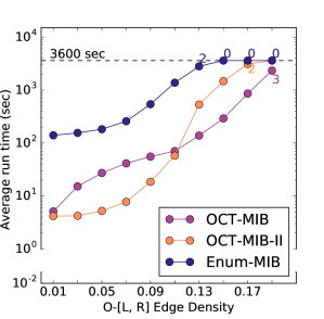
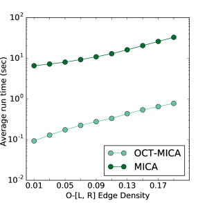
Figure 1: Runtimes of the MIB-enumerating (left) and MB-enumerating (right) algorithms on graphs where $n_{B}=1000$, $n_{L}/n_{R}=10$, and $n_{O}=10$. The expected edge density between $O$ and $L\cup R$ was varied; all other densities were $0.05$.

We implemented OCT-MIB-ii@, Enum-MIB, MICA, and OCT-MICA in C++, and used the implementation of OCT-MIB from [17]. All code is open source under a BSD 3-clause license and publicly available as part of MI-Bicliques at [11].

Data

For convenience, throughout this section, we assume $n_{L}\geq n_{R}$ and let $n_{B}=n_{L}+n_{R}$. Our synthetic data was generated using a modified version of the random graph generator of Zhang et al. [32] that augments random bipartite graphs to have OCT sets of known size. The generator allows a user to specify the sizes of $L$, $R$, and $O$ ($n_{L}$, $n_{R}$, and $n_{O}$), the expected edge densities between $L$ and $R$, $O$ and $L\cup R$, and within $O$, and the coefficient of variation ($cv$; the standard deviation divided by the mean) of the expected number of neighbors in $L$ over $R$ and in $L\cup R$ over $O$. The generator is seeded for replicability. We use the naïve OCT decomposition $[L,R,O]$ returned by the generator for our algorithm evaluation, but the techniques mentioned in Section 2 could also be used to find alternative OCT sets. Unless otherwise specified, the following default parameters are used: expected edge density $\bar{d}=5\%$, $cv=0.5$, $n_{B}=1000$ and $n_{L}/n_{R}=1/10$; additionally, the edge density between $O$ and $L\cup R$ is the same as that between $L$ and $R$.

To add the edges between $L$ and $R$, the edge density and $cv$ values are used to assign vertex degrees to $R$, and then neighbors are selected from $L$ uniformly at random; this was implemented in the generator of [32]. Edges are added between $O$ and $L\cup R$ via the same process, only with the corresponding edge density and $cv$ values. Finally, we add edges within $O$ with an Erdős-Rényi process based on expected density (no $cv$ value is used here).

In most experiments we limit $n_{O}$ to be $O(3\log_{3}n_{B})$, and use a timeout of one hour (3600s). Unless otherwise noted we run each parameter setting with five seeds and plot the average over these instances, using the time-out value as the runtime for instances that don’t finish. If not all instances used for a plot point finished, we annotate it with the number of instances that did not time out.

We began by running our algorithms on the same corpus of graphs as in [17] (see  5.2). As the new algorithms finished considerably faster than those in [17], we were able to scale up both $n_{B}$ and $n_{O}$ to create new sets of experiments, discussed in 5.3. We also ran our algorithms on computational biology graphs from [29], which have been shown to be near-bipartite; these results are in 5.4.

Hardware

All experiments were run on identical hardware; each server had four Intel Xeon E5-2623 v3 CPUs (3.00GHz) and 64GB DDR4 memory. The servers ran Fedora 27 with Linux kernel 4.16.7-200.fc27.x86_64. The C/C++ codes were compiled using gcc/g++ 7.3.1 with optimization flag -O3.

5.2 Initial Benchmarking

We begin by evaluating our algorithms on the corpus of graphs used in [17]. This dataset was designed to independently test the effect of each parameter (the expected densities in various regions of the graph, the $cv$ values, $n_{O}$, $n_{B}$, and $n_{L}/n_{R}$) on the algorithms’ runtime. We observe that OCT-MIB-ii@ and OCT-MICA are generally the best algorithms for their respective problems, and include comprehensive plots of all experiments in the Appendix.

For Maximal Induced Biclique Enumeration, we observe that in general, OCT-MIB-ii@ outperforms OCT-MIB and Enum-MIB. This is the case when the varying parameter is the density within $O$, the $cv$ between $L$ and $R$, the size of the OCT set $n_{O}$, and the ratio between $L$ and $R$, amongst other settings. In these “near-bipartite” synthetic graphs, Enum-MIB unsurprisingly is slowest on most instances. When $n_{B}=1000$ and $n_{O}=3\log_{3}(n_{B})$, Enum-MIB outperforms OCT-MIB when the density within $O$ increases above 0.05. This is likely due to the adverse effect of the number of MISs in the OCT set on OCT-MIB. The most interesting observation occurs when varying the edge density between $O$ and $L\cup R$ (left panel of Figure 1). In the $n_{O}=10$ case, OCT-MIB-ii@ is the fastest algorithm until the density exceeds 0.11, when OCT-MIB becomes faster. We believe this is likely due to OCT-MIB efficiently pruning away attempted expansions which are guaranteed to fail, while the number of MISs in $O$ does not increase. This behavior is also seen in the case where $n_{O}=3\log_{3}n_{B}$, though the magnitude of the difference is not as extreme.

In the non-induced setting of Maximal Biclique Enumeration, OCT-MICA consistently outperforms MICA on this corpus, typically by at least an order of magnitude. The more interesting takeaway is that both MB-enumerating algorithms run considerably faster than their MIB-enumerating counterparts (e.g. right panel of Figure 1), mostly because the number of MIBs is often one to two orders of magnitude larger than the number of MBs in these instances.

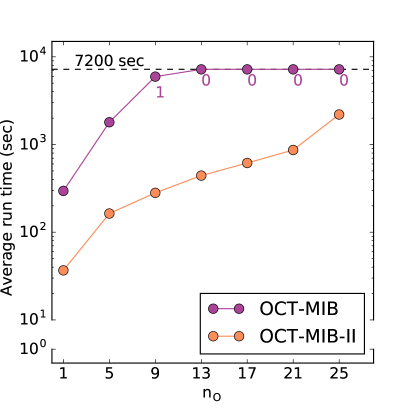
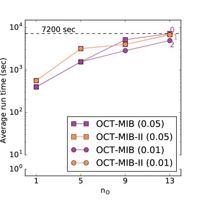
Figure 2: Runtimes of the OCT-based MIB-enumeration algorithms on graphs where $n_{B}=10000$ and $n_{O}$ varies. In the left panel, $n_{L}=9901,n_{R}=99$ ($n_{L}/n_{R}\approx 100$) and the expected edge density is $0.03$. In the right panel, $n_{L}=9091,n_{R}=909$ ($n_{L}/n_{R}\approx 10$) and the expected edge density (excluding within $O$) is $0.01$; the marker-type denotes the expected edge density within $O$ (see legend). For these larger instances we used 3 seeds and a 7200s timeout.

5.3 Larger Graphs

Given the much faster runtimes achieved in Section 5.2 we created a new corpus of larger synthetic graphs. For Maximal Induced Biclique Enumeration, we scaled up $n_{B}$ to 10,000 and varied $n_{O}$ in two settings, increasing the timeout to 7200 seconds. When the expected density was 0.03 and $n_{L}/n_{R}=100$, OCT-MIB-ii@ outperformed OCT-MIB for all values of $n_{O}$ by at least an order of magnitude and finished on all instances, whereas OCT-MIB timed out on all instances with $n_{O}\geq 13$ (left panel of Figure 2). However, when the expected density was 0.01 and $n_{L}/n_{R}=9$, OCT-MIB was faster (right panel of Figure 2). We speculated that this was due to the sparsity of $O$, allowing for a speed-up due to the efficient pruning of OCT-MIB similar to what was seen in Section 5.2. To test this theory, we increased expected edge density within $O$ to 0.05 while leaving the other parameters the same (right panel of Figure 2), and observed that once $n_{O}\geq 9$, OCT-MIB-ii@ outperforms OCT-MIB, confirming our hypothesis.

For Maximal Biclique Enumeration, we also designed a new experiment where $n_{B}=10000$ and $n_{O}$ was scaled up to 1000 (left panel of Figure 3). OCT-MICA finished on all instances, whereas MICA finished on none when $n_{O}$ was 1000. We also tested how large we could scale the expected density between $L$ and $R$ (right panel of Figure 3). When $n_{B}=100$, OCT-MICA finished on all instances with density at most 0.4, while MICA finished on two of five when density is 0.4. Neither algorithm finished in less than the timeout of an hour when the density was 0.5 or greater, exhausting the hardware’s memory in many cases. Thus OCT-MICA is able to scale to graphs with considerably larger OCT sets and higher density than both MICA and the MIB-enumerating algorithms.

We additionally created graphs with $n_{O}>3\log_{3}n_{B}$, which was not done in [17], and ran the algorithms for both MIBs and MBs (Figure 4). These graphs had $n_{B}$ values up to 4000 and for each value of $n_{B}$, we used three values of $n_{O}$; $10,3\log_{3}n_{B},$ and $\sqrt{n_{B}}$. The results were most interesting for the MIB-enumerating algorithms (Figure 4 top). OCT-MIB performed the worst of the three algorithms when $n_{O}=\sqrt{n_{B}}$, but outperformed Enum-MIB in the other settings. This verifies the analysis from [17] on the range in which OCT-MIB is most effective. In general, OCT-MIB-ii@ once again was the fastest algorithm and did best when $n_{O}$ was smaller. The impact of $n_{O}$ on OCT-MIB-ii@ and Enum-MIB appeared comparable. In the MB-enumeration case, OCT-MICA consistently outperforms MICA, and there is a distinguishable difference in the runtime based on the value of $n_{O}$ (Figure 4 bottom). The value of $n_{O}$ has far less effect on MICA, which does not finish on any graphs with $n_{B}=4000$.

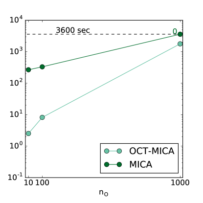
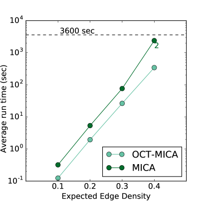
Figure 3: Runtimes of the MB-enumerating algorithms on graphs with larger $n_{B}$ and expected edge density. In the left panel, $n_{L}=9091,n_{R}=909$ ($n_{L}/n_{R}\approx 10$), the expected edge density is $0.05$, and $n_{O}$ varied. In the right panel, $n_{L}=91,n_{R}=9$ ($n_{L}/n_{R}\approx 10$), $n_{O}=50$, and the expected edge density varied.

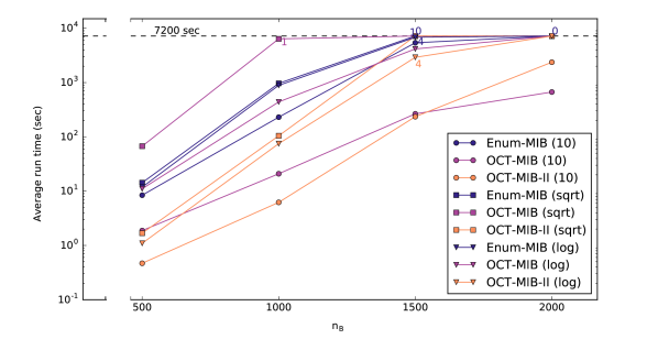
(a)

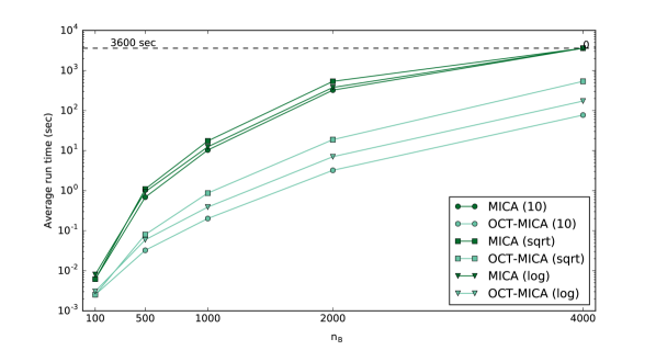
(b)

Figure 4: Runtimes of the MIB-enumerating (top) and MB-enumerating (bottom) algorithms on graphs where $n_{L}/n_{R}=9$ and all expected edge densities are $0.05$. $n_{B}$ is varied (x-axis) and the marker-type denotes the value of $n_{O}\in\{10,\sqrt{n_{B}},3\log_{3}(n_{B})\}$ (see legend). The time-out value is set to 7200s for the MIB-enumerating algorithms and 3600s for the MB-enumerating algorithms.

5.4 Computational Biology Data

Finally, we tested performance on real-world data using the graphs from [29], which come from computational biology. These graphs have previously been exhibited to have small OCT sets [12], and we used the implementation from [9] of Hüffner’s iterative compression algorithm [12] to find the OCT decompositions. Computing the OCT decomposition for each graph ran in less than ten seconds, and often in less than one second. As can be seen in Table 1, OCT-MIB-ii@ performs the best of the MIB-enumerating algorithms and OCT-MICA is faster than MICA. Full results are in the Appendix.

$G$	$n_{B}$	$m$	$n_{O}$	$|M_{I}|$	OCT-MIB-ii@	OCT-MIB	Enum-MIB	$|M_{B}|$	OCT-MICA	MICA
aa-24	258	1108	21	3890	2.108	9.140	14.167	1334	0.237	2.477
aa-30	39	71	4	56	0.002	0.007	0.006	36	0.002	0.007
aa-41	296	1620	40	11705	16.519	82.439	50.205	20375	9.059	47.789
aa-50	113	468	18	1272	0.322	0.778	1.098	1074	0.132	0.612
j-20	241	640	1	274	0.013	0.065	0.484	228	0.009	0.188
j-24	142	387	4	150	0.013	0.027	0.089	104	0.007	0.025

Table 1: A sampling of the runtimes of the biclique-enumeration algorithms on the Wernicke-Hüffner computational biology data [29].

6 Conclusion

We present a suite of new algorithms for enumerating maximal (induced) bicliques in general graphs, two of which are parameterized by the size of an odd cycle transversal. It is particularly noteworthy that the parameterized algorithms empirically outperform the general approaches even when their asymptotic worst-case complexities are worse. This highlights a weakness of standard complexity analysis, as many aspects of an algorithm get “swept under the rug”.

It is also interesting that even though Maximal Induced Biclique Enumeration and Maximal Biclique Enumeration are closely related problems, the MB-enumerating algorithms are often an order of magnitude faster than their MIB-enumerating counterparts. The reason for this can likely be attributed to two causes: the number of MBs is significantly less than the number of MIBs in sparse graphs, and that the stricter structure of MIBs requires more work to ensure. For $S\subseteq V$, there is exactly one MB of the form $S\times T\subseteq V$ in $G$, but there can be many MIBs with this structure.

We implement and benchmark all of the algorithms on a corpus of synthetic and real-world computational biology graphs, and establish that parameterized approaches are often at least an order of magnitude faster than the general approaches. This remains true even when $n_{O}\in O(\sqrt{n})$. It would be interesting to experimentally evaluate as $n_{O}$ increases, at what point the standard methods outperform those optimized for near-bipartite graphs. Finally, we note as in  [17], the current implementations of the algorithms could be improved by replacing the MIS-enumeration algorithm with that of [28], and the M(I)B-enumeration on bipartite graphs with the implementation used in [32].

Appendices

Appendix 0.A MIB-Enumeration Framework Subroutines

We now provide algorithmic details and proofs of the complexity and correctness of MakeIndMaximal and AddTo.

0.A.1 MakeIndMaximal

Recall that MakeIndMaximal takes in $(C,S)$, where $C$ is an induced biclique and $S\subseteq V$, and either returns a MIB $C^{+}$ where $C\subseteq C^{+}$, $C^{+}\subseteq C\cup S$, $C\neq\emptyset$, or returns $\emptyset$. If it returns $\emptyset$ and $C\neq\emptyset$ then there is another MIB $D$ which contains $C$ and $v\in(V\setminus S)\setminus C$. We give pseudo-code of MakeIndMaximal in Algorithm 3.

1:Input: $G=(V,E)$, $C=C_{1}\times C_{2}$, $S$

2:Let $C_{S}=S\setminus(C_{1}\cup C_{2})$

3:if $C==\emptyset$ then

4:     return $\emptyset$

5:for $v\in C_{S}$ do

6:     if $|N(v)\cap C_{1}|==|C_{1}|\And|N(v)\cap C_{2}|==0$ then

7:         $C_{2}=C_{2}\cup\{v\}$

8:         $C_{S}\setminus\{v\}$      

9:for $v\in C_{S}$ do

10:     if $|N(v)\cap C_{2}|==|C_{2}|\And|N(v)\cap C_{1}|==0$ then

11:         $C_{1}=C_{1}\cup\{v\}$      

12:$V_{S}=V\setminus(S\cup C_{1}\cup C_{2})$

13:for $v\in V_{S}$ do

14:     if $|N(v)\cap C_{1}|==|C_{1}|\And|N(v)\cap C_{2}|==0$ then

15:         return $\emptyset$      

16:for $v\in V_{S}$ do

17:     if $|N(v)\cap C_{2}|==|C_{2}|\And|N(v)\cap C_{1}|==0$ then

18:         return $\emptyset$      

19:return $C^{+}=C_{1}\times C_{2}$

Algorithm 3 MakeIndMaximal

Lemma 5

MakeIndMaximal returns a MIB $C^{+}$ where $C\subseteq C^{+}$, $C^{+}\subseteq C\cup S$, $C\neq\emptyset$, or returns $\emptyset$.

Proof

Referring to the pseudo-code in Algorithm 3, it is clear that $C\subseteq C^{+}$, as no vertices are ever removed from the input biclique $C$. Furthermore, the only vertices added to $C^{+}$ are from $S$, so $C^{+}\subseteq C\cup S$ and $C^{+}$ is the only biclique returned by MakeIndMaximal. Note that neither side of $C$ is empty and the only vertices added are independent from the side of the biclique which they are added to, so if we do not return $\emptyset$ the object returned is an induced biclique. If no node from outside of $S$ can be added to $C^{+}$, then we will not return $\emptyset$ and thus $C^{+}$ is maximal.

Lemma 6

If MakeIndMaximal returns $\emptyset$ and $C\neq\emptyset$ then there is another MIB $D$ in $G$ which contains $C$ and $v\in(V\setminus S)\setminus C$.

Proof

Note that $C\subseteq C^{*}=C_{1}\times C_{2}$ at line 12. As MakeIndMaximal returns $\emptyset$ there must be a vertex $v\in V_{S}=V\setminus(S\cup C^{*})$ which can be added to $C^{*}$. Let $D$ be a MIB containing $C^{*}$ and $v$, thus $D$ suffices to prove the lemma.

Lemma 7

MakeIndMaximal runs in $O(m)$ time.

Proof

Note that because $G$ is connected, $n\in O(m)$. Setting $C_{S}$ and $V_{S}$ can be done in $O(n)$ time. In each for loop, we can scan all of the edges incident to each $v$ in the iterated-over set and keep count of how many nodes from $C_{i}$ have been seen (checking for inclusion can be done in $O(1)$ time with an $O(n)$ initialization step). Thus, each edge is scanned at most once per for loop.

0.A.2 AddTo

Recall that AddTo takes in $(C,v)$ where $C=C_{1}\times C_{2}$ is an induced biclique and $v\in V\setminus(C_{1}\cup C_{2})$, and returns the induced biclique where $v$ is added to $C_{1}$, $N(v)$ is removed from $C_{1}$, and $\overline{N}(v)$ is removed from $C_{2}$ if $C_{2}\setminus\overline{N}(v)\neq\emptyset$ and $\emptyset$ otherwise. We give pseudo-code of AddTo in Algorithm 4.

1:Input: $G=(V,E)$, $C=C_{1}\times C_{2}$, $v\in V\setminus(C_{1}\cup C_{2})$

2:$C_{1}^{\prime}=(C_{1}\cup\{v\})\setminus N(v)$

3:$C_{2}^{\prime}=C_{2}\cap{N(v)}$

4:if $C_{2}^{\prime}==\emptyset$ then

5:     return $\emptyset$

6:return $C_{1}^{\prime}\times C_{2}^{\prime}$

Algorithm 4 AddTo

Lemma 8

AddTo returns the induced biclique where $v$ is added to $C_{1}$, $N(v)$ is removed from $C_{1}$, and $\overline{N}(v)$ is removed from $C_{2}$ if $C_{2}\setminus\overline{N}(v)\neq\emptyset$, and $\emptyset$ otherwise.

Proof

Referring to the pseudo-code in Algorithm 4, it is clear that $v$ is added to $C_{1}$ and $N(v)$ is removed from $C_{1}$. Additionally $v$’s non-neighbors are effectively removed from $C_{2}$ by intersecting it with $N(v)$. If $C_{2}^{\prime}=\emptyset$ then $C_{2}\setminus\overline{N}(v)=\emptyset$ and $\emptyset$ is returned. Otherwise $C_{1}^{\prime}\neq\emptyset$ since it includes $v$ and thus $C_{1}^{\prime}\times C_{2}^{\prime}$ is a biclique. $C_{1}^{\prime}\times C_{2}^{\prime}$ must be an induced biclique as $C_{2}^{\prime}\subseteq C_{2}$, $C_{1}^{\prime}\setminus\{v\}\subseteq C_{1}$, and $C_{1}\times C_{2}$ is an induced biclique and $(N(v)\cap C_{1}^{\prime})=\emptyset$ by definition.

Lemma 9

AddTo runs in $O(m)$ time.

Proof

Note that because $G$ is connected, $n\in O(m)$. AddTo can be completed by scanning all of $v$’s $O(m)$ incident edges in tandem with an $O(n)$ preprocessing step to allow for constant-time look-ups when checking for inclusion in a set.

Appendix 0.B MB-Enumeration Framework Subroutines

We give a detailed description of the MakeMaximal and Consensus subroutines used in OCT-MICA, along with arguments of their correctness and complexity.

0.B.1 MakeMaximal

Extending a biclique to be maximal is different in the non-induced case from the induced case, since MBs are completely characterized by one side of the biclique.

Algorithm 5 MakeMaximal

1:Input: $G=(V,E)$, $B=X\times Y$

2:$X^{*}=\cap_{i\in Y}N(i)$

3:$Y^{*}=\cap_{i\in X^{*}}N(i)$

4:return $B^{*}=X^{*}\times Y^{*}$

Lemma 10

MakeMaximal runs in $O(m)$ time.

Proof

In order to form $X^{*}$, we can scan the edges incident to each $v\in Y$ and keep count of how many nodes from $X^{*}$ have been seen (checking for inclusion can be done in $O(1)$ time with an $O(n)$ initialization step). The same can be done for $Y^{*}$, where instead we scan the edges incident to each $v\in X^{*}$. Thus, each edge is scanned at most twice in MakeMaximal.

0.B.2 Consensus

The MICA section of OCT-MICA relies heavily on the Consensus operation introduced in [3] for finding new candidate bicliques. For each pair of bicliques, there are four candidate bicliques which form the consensus of the pair. Note that any of the four candidates may be empty and if so discarded. Consensus runs in $O(n)$ time using standard techniques for set union and intersection.

Algorithm 6 Consensus

1:Input: $G=(V,E)$, $B_{\alpha}=X_{\alpha}\times Y_{\alpha}$, $B_{\beta}=X_{\beta}\times Y_{\beta}$

2:$B_{1}=(X_{\alpha}\cup X_{\beta})\times(Y_{\alpha}\cap Y_{\beta})$

3:$B_{2}=(X_{\alpha}\cap X_{\beta})\times(Y_{\alpha}\cup Y_{\beta})$

4:$B_{3}=(Y_{\alpha}\cup X_{\beta})\times(X_{\alpha}\cap Y_{\beta})$

5:$B_{4}=(X_{\alpha}\cap Y_{\beta})\times(Y_{\alpha}\cup X_{\beta})$

6:$S=\{\}$

7:for $B_{i}=X_{i}\times Y_{i}\in\{B_{1},B_{2},B_{3},B_{4}\}$ do

8:     if $|X_{i}|>0\And|Y_{i}|>0$ then

9:         $S$.add($B_{i}$)      

10:return $S$

Appendix 0.C Additional Enumeration Experiments

Here we include figures corresponding to additional experimental results of our initial benchmarking and on the computation biology data from [29] described in sections 5.2 and 5.4 respectively.

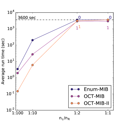
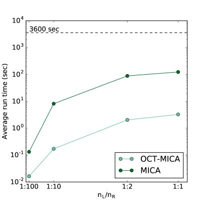
Figure 5: Runtimes of the MIB-enumerating (left) and MB-enumerating (right) algorithms on graphs where $n_{B}=1000$ and $n_{O}=10$. The ratio $n_{L}/n_{R}$ was varied.

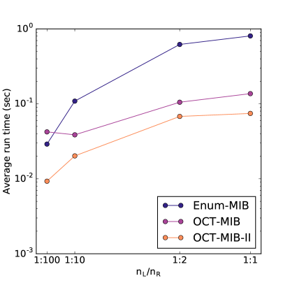
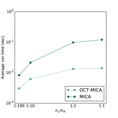
Figure 6: Runtimes of the MIB-enumerating (left) and MB-enumerating (right) algorithms on graphs where $n_{B}=200$ and $n_{O}=10$. The ratio $n_{L}/n_{R}$ was varied.

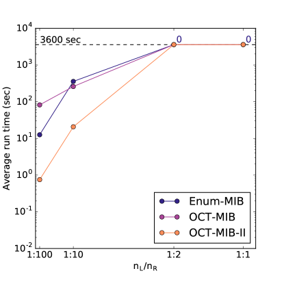
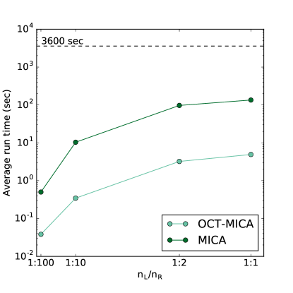
Figure 7: Runtimes of the MIB-enumerating (left) and MB-enumerating (right) algorithms on graphs where $n_{B}=1000$ and $n_{O}=19\approx 3\log_{3}(n_{B})$. The ratio $n_{L}/n_{R}$ was varied.

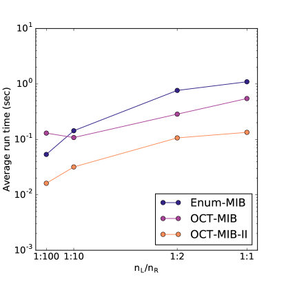
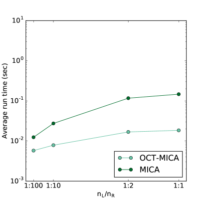
Figure 8: Runtimes of the MIB-enumerating (left) and MB-enumerating (right) algorithms on graphs where $n_{B}=200$ and $n_{O}=14\approx 3\log_{3}(n_{B})$. The ratio $n_{L}/n_{R}$ was varied.

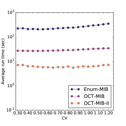
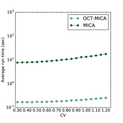
Figure 9: Runtimes of the MIB-enumerating (left) and MB-enumerating (right) algorithms on graphs where $n_{B}=1000$ and $n_{O}=10$. The coefficient of variation between $L$ and $R$ was varied.

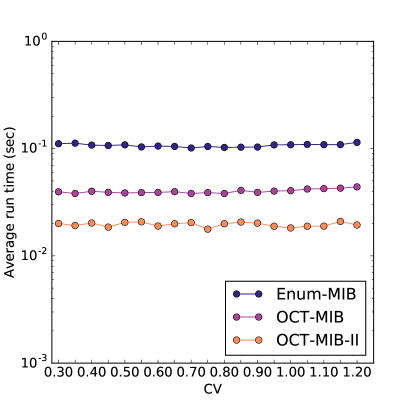
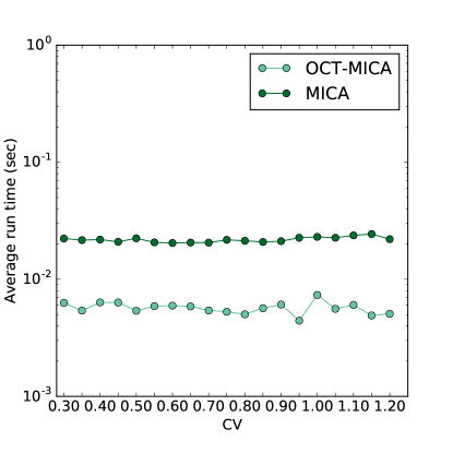
Figure 10: Runtimes of the MIB-enumerating (left) and MB-enumerating (right) algorithms on graphs where $n_{B}=200$ and $n_{O}=10$. The coefficient of variation between $L$ and $R$ was varied.

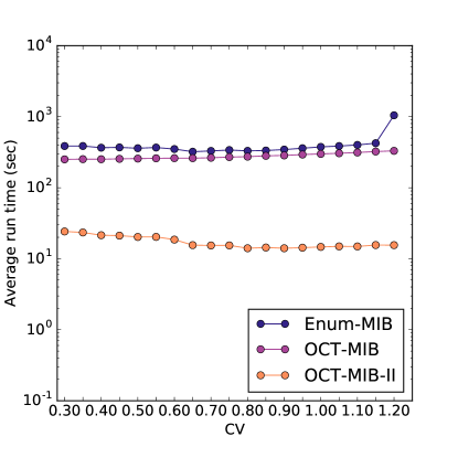
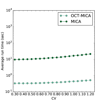
Figure 11: Runtimes of the MIB-enumerating (left) and MB-enumerating (right) algorithms on graphs where $n_{B}=1000$ and $n_{O}=19\approx 3\log_{3}(n_{B})$. The coefficient of variation between $L$ and $R$ was varied.

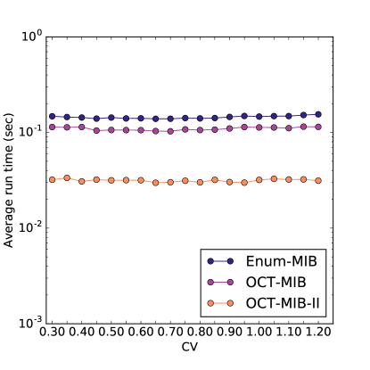
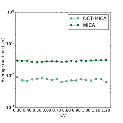
Figure 12: Runtimes of the MIB-enumerating (left) and MB-enumerating (right) algorithms on graphs where $n_{B}=200$ and $n_{O}=14\approx 3\log_{3}(n_{B})$. The coefficient of variation between $L$ and $R$ was varied.

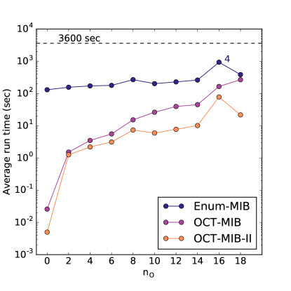
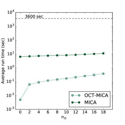
Figure 13: Runtimes of the MIB-enumerating (left) and MB-enumerating (right) algorithms on graphs where $n_{B}=1000$ and $n_{O}$ was varied.

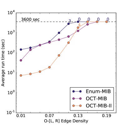
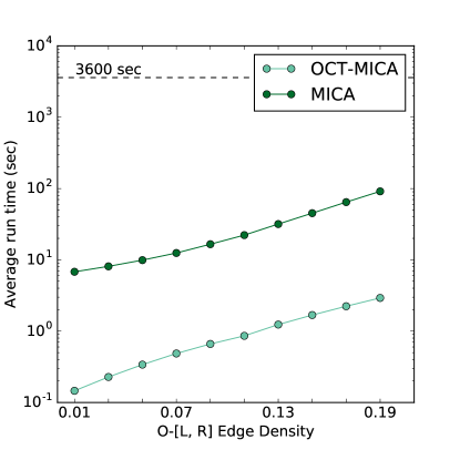
Figure 14: Runtimes of the MIB-enumerating (left) and MB-enumerating (right) algorithms on graphs where $n_{B}=1000$ and $n_{O}=19\approx 3\log_{3}(n_{B})$. The expected edge density between $O$ and $\{L,R\}$ was varied.

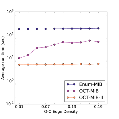
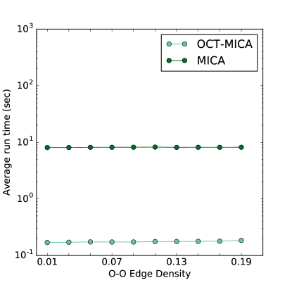
Figure 15: Runtimes of the MIB-enumerating (left) and MB-enumerating (right) algorithms on graphs where $n_{B}=1000$ and $n_{O}=10$. The expected edge density within $O$ was varied.

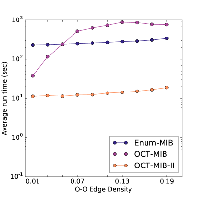
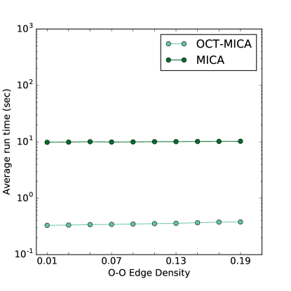
Figure 16: Runtimes of the MIB-enumerating (left) and MB-enumerating (right) algorithms on graphs where $n_{B}=1000$ and $n_{O}=19\approx 3\log_{3}(n_{B})$. The expected edge density within $O$ was varied.

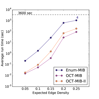
Figure 17: Runtimes of the MIB-enumerating (left) and MB-enumerating (right) algorithms on graphs where $n_{B}=150$, $n_{L}=n_{R}$ and $n_{O}=5$. The expected edge density in the graph was varied except for the expected edge density within $O$ which was fixed to $0.05$.

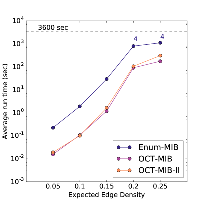
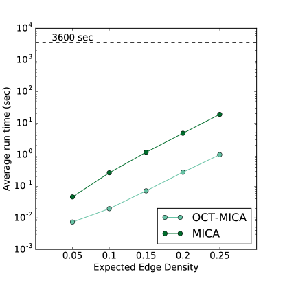
Figure 18: Runtimes of the MIB-enumerating (left) and MB-enumerating (right) algorithms on graphs where $n_{B}=150$, $n_{L}=n_{R}$ and $n_{O}=5$. The expected edge density in the graph was varied, including the expected edge density within $O$.

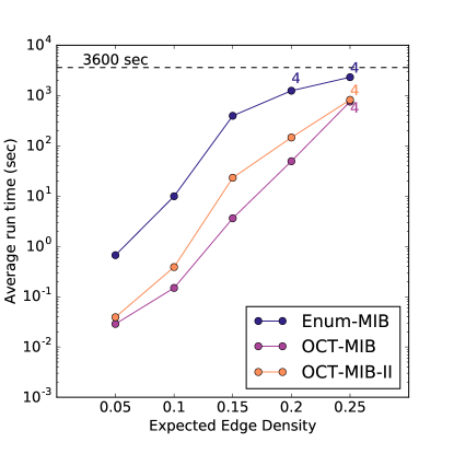
Figure 19: Runtimes of the MIB-enumerating (left) and MB-enumerating (right) algorithms on graphs where $n_{B}=200$, $n_{L}=n_{R}$ and $n_{O}=5$. The expected edge density in the graph was varied except for the expected edge density within $O$ which was fixed to $0.05$.

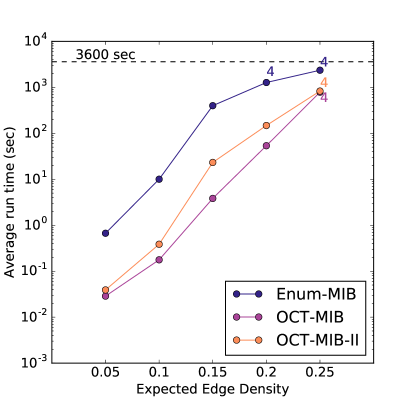
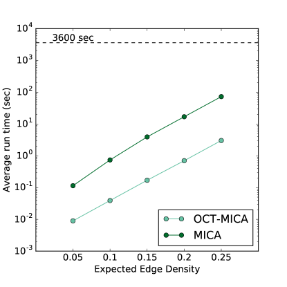
Figure 20: Runtimes of the MIB-enumerating (left) and MB-enumerating (right) algorithms on graphs where $n_{B}=200$, $n_{L}=n_{R}$ and $n_{O}=5$. The expected edge density in the graph was varied, including the expected edge density within $O$.

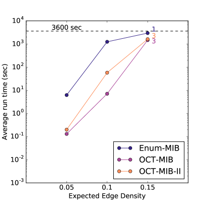
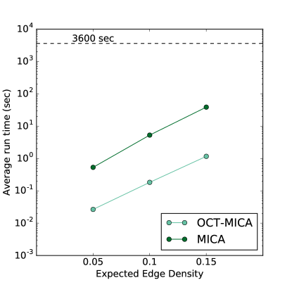
Figure 21: Runtimes of the MIB-enumerating (left) and MB-enumerating (right) algorithms on graphs where $n_{B}=300$, $n_{L}=n_{R}$ and $n_{O}=5$. The expected edge density in the graph was varied except for the expected edge density within $O$ which was fixed to $0.05$.

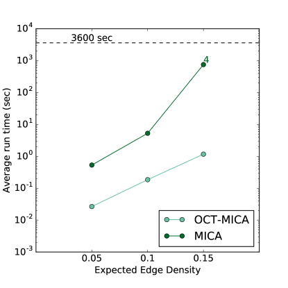
Figure 22: Runtimes of the MIB-enumerating (left) and MB-enumerating (right) algorithms on graphs where $n_{B}=300$, $n_{L}=n_{R}$ and $n_{O}=5$. The expected edge density in the graph was varied, including the expected edge density within $O$.

$G$	$n_{B}$	$m$	$n_{O}$	$|M_{I}|$	OCT-MIB-ii@	OCT-MIB	Enum-MIB	$|M_{B}|$	OCT-MICA	MICA
aa-10	69	191	6	178	0.008	0.023	0.057	98	0.007	0.031
aa-11	102	307	11	424	0.055	0.115	0.259	206	0.018	0.120
aa-13	129	383	12	523	0.083	0.239	0.470	269	0.028	0.166
aa-14	125	525	19	1460	0.366	0.902	1.254	605	0.090	0.485
aa-15	66	179	7	206	0.010	0.019	0.053	113	0.011	0.030
aa-16	13	15	0	15	0.000	0.000	0.000	8	0.000	0.000
aa-17	151	633	25	2252	1.023	2.132	3.457	1250	0.242	1.137
aa-18	87	381	14	660	0.100	0.173	0.389	823	0.090	0.351
aa-19	191	645	19	1262	0.449	1.569	2.385	519	0.069	0.450
aa-20	224	766	19	1607	0.705	2.431	3.809	949	0.154	1.061
aa-21	28	90	9	116	0.006	0.013	0.008	213	0.019	0.030
aa-22	167	641	16	1520	0.423	1.387	2.629	560	0.074	0.638
aa-23	139	508	18	1766	0.435	0.788	1.651	1530	0.210	1.000
aa-24	258	1108	21	3890	2.108	9.140	14.167	1334	0.237	2.477
aa-25	14	15	1	10	0.000	0.001	0.001	10	0.000	0.000
aa-26	92	284	13	583	0.084	0.186	0.309	370	0.030	0.128
aa-27	118	331	11	458	0.054	0.270	0.343	229	0.015	0.114
aa-28	167	854	27	2606	1.464	2.201	4.162	2814	0.755	3.250
aa-29	276	1058	21	3122	1.909	8.418	10.707	1924	0.382	3.344
aa-30	39	71	4	56	0.002	0.007	0.006	36	0.002	0.007
aa-31	30	51	2	37	0.002	0.002	0.002	22	0.001	0.002
aa-32	143	750	30	4167	2.286	7.694	5.290	3154	0.684	2.635
aa-33	193	493	4	578	0.046	0.204	0.993	218	0.012	0.218
aa-34	133	451	13	705	0.132	0.316	0.756	275	0.031	0.226
aa-35	82	269	10	459	0.037	0.108	0.178	215	0.019	0.081
aa-36	111	316	7	248	0.015	0.076	0.155	143	0.011	0.078
aa-37	72	170	5	135	0.005	0.018	0.054	82	0.005	0.022
aa-38	171	862	26	4270	2.428	5.223	7.586	4964	1.136	5.179
aa-39	144	692	23	2153	0.872	1.574	3.034	1177	0.237	1.009
aa-40	136	620	22	2727	1.022	2.086	2.973	1911	0.301	1.324
aa-41	296	1620	40	11705	16.519	82.439	50.205	20375	9.059	47.789
aa-42	236	1110	30	6967	5.646	45.560	21.244	8952	2.428	13.479
aa-43	63	308	18	905	0.137	0.294	0.311	875	0.116	0.302
aa-44	59	163	10	211	0.014	0.024	0.051	158	0.008	0.037
aa-45	80	386	20	1768	0.336	0.775	0.859	1716	0.244	0.796
aa-46	161	529	13	719	0.157	0.438	0.922	374	0.036	0.257
aa-47	62	229	14	572	0.057	0.082	0.138	451	0.051	0.127
aa-48	89	343	17	896	0.144	0.338	0.497	519	0.060	0.230
aa-49	26	62	5	50	0.004	0.002	0.003	74	0.006	0.013
aa-50	113	468	18	1272	0.322	0.778	1.098	1074	0.132	0.612
aa-51	78	274	11	429	0.035	0.082	0.174	250	0.020	0.078
aa-52	65	231	14	690	0.073	0.135	0.200	431	0.040	0.122
aa-53	88	232	12	340	0.036	0.186	0.162	199	0.011	0.052
aa-54	89	233	12	286	0.027	0.063	0.113	177	0.015	0.039

Table 2: The runtimes (rounded to nearest thousandth-of-a-second) of the biclique-enumeration algorithms on the Afro-American subset of the Wernicke-Hüffner computational biology data [29].

$G$	$n_{B}$	$m$	$n_{O}$	$|M_{I}|$	OCT-MIB-ii@	OCT-MIB	Enum-MIB	$|M_{B}|$	OCT-MICA	MICA
j-10	55	117	3	52	0.002	0.009	0.010	39	0.001	0.010
j-11	51	212	5	63	0.003	0.014	0.011	36	0.003	0.012
j-13	78	210	6	224	0.015	0.028	0.074	90	0.009	0.032
j-14	60	107	4	44	0.004	0.007	0.003	38	0.003	0.003
j-15	44	55	1	13	0.001	0.000	0.004	10	0.001	0.000
j-16	9	10	0	10	0.000	0.000	0.000	3	0.000	0.000
j-17	79	322	10	317	0.025	0.051	0.127	126	0.014	0.056
j-18	71	296	9	154	0.011	0.038	0.053	91	0.012	0.028
j-19	84	172	3	105	0.002	0.010	0.019	46	0.002	0.013
j-20	241	640	1	274	0.013	0.065	0.484	228	0.009	0.188
j-21	33	102	9	107	0.006	0.012	0.008	197	0.017	0.024
j-22	75	391	9	221	0.020	0.051	0.080	113	0.009	0.048
j-23	76	369	19	682	0.095	0.404	0.217	459	0.057	0.132
j-24	142	387	4	150	0.013	0.027	0.089	104	0.007	0.025
j-25	14	14	0	14	0.000	0.000	0.000	3	0.000	0.000
j-26	63	156	6	156	0.007	0.019	0.035	67	0.003	0.013
j-28	90	567	13	492	0.073	0.130	0.244	416	0.044	0.193

Table 3: The runtimes (rounded to nearest thousandth-of-a-second) of the biclique-enumeration algorithms on the Japanese subset of the Wernicke-Hüffner computational biology data [29].

References

- [1] P. Agarwal, N. Alon, B. Aronov, and S. Suri, Can visibility graphs be represented compactly?, Discrete & Computational Geometry, 12 (1994), pp. 347–365.
- [2] T. Akiba and Y. Iwata, Branch-and-reduce exponential/fpt algorithms in practice: A case study of vertex cover, Theoretical Computer Science, 609 (2016), pp. 211–225.
- [3] G. Alexe, S. Alexe, Y. Crama, S. Foldes, P. Hammer, and B. Simeone, Consensus algorithms for the generation of all maximal bicliques, Discrete Applied Mathematics, 145 (2004), pp. 11–21.
- [4] M. Dawande, P. Keskinocak, J. Swaminathan, and S. Tayur, On bipartite and multipartite clique problems, J. of Algorithms, 41(2001), pp. 388–403.
- [5] V. Dias, C. De Figueiredo, and J. Szwarcfiter, Generating bicliques of a graph in lexicographic order, Theoretical Computer Science, 337 (2005), pp. 240–248.
- [6] D. Eppstein, Arboricity and bipartite subgraph listing algorithms, Inf. Process. Lett., 51 (1994), pp. 207–211.
- [7] M. Garey and D. Johnson, Computers and intractability: a guide to NP-completeness, 1979.
- [8] A. Gély, L. Nourine, and B. Sadi, Enumeration aspects of maximal cliques and bicliques, Discrete Applied Mathematics, 157(7), (2009) pp. 1447–1459.
- [9] T. Goodrich, E. Horton, and B. Sullivan, Practical Graph Bipartization with Applications in Near-Term Quantum Computing, arXiv preprint arXiv:1805.01041, 2018.
- [10] N. Gülpinar, G. Gutin, G. Mitra, and A. Zverovitch, Extracting pure network submatrices in linear programs using signed graphs, Discrete Applied Mathematics, 137 (2004), pp. 359–372.
- [11] E. Horton, K. Kloster, B. D. Sullivan, A. van der Poel, MI-bicliques, https://github.com/TheoryInPractice/MI-bicliques, October 2018.
- [12] F. Hüffner, Algorithm engineering for optimal graph bipartization, International Workshop on Experimental and Efficient Algorithms, 2005, pp. 240–252.
- [13] W. Chang, Maximal Biclique Enumeration, http://genome.cs.iastate.edu/supertree/download/biclique/README.html, December 2004
- [14] Y. Iwata, K. Oka, and Y. Yoshida, Linear-time FPT algorithms via network flow, SODA, 2014, pp. 1749–1761.
- [15] M. Kaytoue-Uberall, S. Dupelessis, and A. Napoli, Using formal concept analysis for the extraction of groups of co-expressed genes, Modelling, Computation and Optimization in Information Systems and Management Sciences, 2008, pp. 439–449.
- [16] M. Kaytoue, S. Kuznetsov, A. Napoli, and S. Duplessis, Mining gene expression data with pattern structures in formal concept analysis, Information Sciences, 181 (2011), pp. 1989–2011.
- [17] K. Kloster, B. Sullivan, and A. van der Poel, Mining Maximal Induced Bicliques using Odd Cycle Transversals, Proceedings of the 2019 SIAM International Conference on Data Mining, 2019 (to appear).
- [18] R. Kumar, P. Raghavan, S. Rajagopalan, and A. Tomkins, Trawling the Web for emerging cyber-communities, Computer Networks, 31 (1999), pp. 1481–1493.
- [19] S. Kuznetsov, On computing the size of a lattice and related decision problems, Order, 18 (2001), pp. 313–321.
- [20] J. Li, G. Liu, H. Li, and L. Wong, Maximal biclique subgraphs and closed pattern pairs of the adjacency matrix: A one-to-one correspondence and mining algorithms, IEEE Trans. Knowl. Data Eng., 19 (2007), pp. 1625–1637.
- [21] D. Lokshtanov, S. Saurab, and S. Sikdar, Simpler parameterized algorithm for OCT, International Workshop on Combinatorial Algorithms, 2009, pp. 380–384.
- [22] K. Makino and T. Uno, New algorithms for enumerating all maximal cliques, Scandinavian Workshop on Algorithm Theory, 2004, pp. 260–272.
- [23] R. Mushlin, A. Kershenbaum, S. Gallagher, and T. Rebbeck, A graph-theoretical approach for pattern discovery in epidemiological research, IBM Systems J., 46 (2007), pp. 135–149.
- [24] A. Panconesi and M. Sozio, Fast hare: A fast heuristic for single individual SNP haplotype reconstruction, International workshop on algorithms in bioinformatics, 2004, pp. 266–277.
- [25] R. Peeters, The maximum edge biclique problem is NP-complete, Discrete Applied Mathematics, 131 (2003), pp. 651–654.
- [26] M. Sanderson, A. Driskell, R. Ree, O. Eulenstein, and S. Langley, Obtaining maximal concatenated phylogenetic data sets from large sequence databases, Molecular Biology and Evolution, 20 (2003), pp. 1036–1042.
- [27] J. Schrook, A. McCaskey, K. Hamilton, T. Humble, and N. Imam, Recall Performance for Content-Addressable Memory Using Adiabatic Quantum Optimization Entropy, 19 (2017).
- [28] S. Tsukiyama, M. Ide, H. Ariyoshi, and I. Shirakawa, A new algorithm for generating all the maximal independent sets, SIAM J. on Computing, 6 (1977), pp. 505–517.
- [29] S. Wernicke, On the algorithmic tractability of single nucleotide polymorphism (SNP) analysis and related problems, 2014.
- [30] R. Wille, Restructuring lattice theory: an approach based on hierarchies of concepts, Ordered sets, 1982, pp. 445–470.
- [31] M. Yannakakis, Node-and edge-deletion NP-complete problems, STOC, 1978, pp. 253–264.
- [32] Y. Zhang, C. A. Phillips, G. L. Rogers, E. J. Baker, E. J. Chesler, and M. A. Langston, On finding bicliques in bipartite graphs: a novel algorithm and its application to the integration of diverse biological data types, BMC Bioinformatics, 15 (2014).