Cosmic expansion from spinning black holes

Abstract

We examine how cosmological expansion arises in a universe containing a lattice of spinning black holes. We study averaged expansion properties as a function of fundamental properties of the black holes, including the bare mass of the black holes and black hole spin. We then explore how closely the expansion properties correspond to properties of a corresponding matter-dominated FLRW universe. As residual radiation present in the initial data decays, we find good agreement with a matter-dominated FLRW solution, and the effective density in the volume is well-described by the horizon mass of the black hole.

1 Introduction

Cosmological systems are often modeled as perturbations around a homogeneous, isotropic Friedmann-Lemaître-Robertson-Walker (FLRW) spacetime where the background dynamics are described by homogeneous and isotropic stress-energy sources. Yet, the homogeneity of the stress-energy tensor is manifestly broken on smaller length scales where discrete objects exist, and inhomogeneous structures and well-isolated astrophysical systems predominate. A notion of homogeneity and isotropy can still be recovered through averaging, in which small-scale structures in the Universe are coarse-grained and an effective FLRW cosmology emerges. Observations support the picture that we live in an approximately homogeneous and isotropic FLRW universe[1, 2]; what remains uncertain is the precise relationship between the actual Universe, with its extreme inhomogeneity on many scales, and the perturbed homogeneous isotropic cosmology we use as a model.

In recent years, numerical studies have begun to explore some of the differences between these pictures[3, 4], giving rise to many questions including: how do beams of light and gravitational waves propagate in a warped cosmological vacuum rather than a perturbed perfect fluid[5, 6]? What microphysics best describes the manner in which isolated objects contribute to global cosmological expansion?

In this work, we begin to examine the latter of these questions by simulating a lattice of spinning black holes and examining properties of the spacetime, which is shown to develop an overall average FLRW-like cosmological expansion. Black hole lattice models have been employed as toy models for cosmological systems in order to ask such questions in the past [5, 6, 7, 8, 9, 10, 11, 12] (and see [13] for a recent review), and these models and similar semianalytic models have been able to provide insights into both the physics of spatial hypersurfaces in these models and, more recently, observables [14, 15, 16]. Such models have been found to reproduce FLRW-type behavior with varying degrees of fidelity, with properties that depend on the precise details of the inhomogeneous structure [17, 18, 19, 20]. This dependence is interesting in and of itself, as it suggests that the cosmological properties of inhomogeneous spacetimes do not always provide insight into the more fundamental small-scale properties of a spacetime. For example, different measures of the mass contained within these spacetimes have been found to disagree by orders of magnitude: some definitions of mass appear to coincide with FLRW expectations, while others do not [21, 7, 22].

Here we extend these models to a lattice of spinning (rather than purely static) black holes. We lay down initial conditions and follow the subsequent evolution of the spacetime using numerical general-relativistic simulations. For black holes parametrized by a given mass and spin, we examine the expansion rate within the box, and explore how different energy components contribute to cosmological expansion. Although we do not calculate cosmological observables here, this work lays down the foundation for a series of future work regarding observational consequences.

We first describe our procedure for setting initial conditions with a spinning black hole in a periodic spacetime in Section 2. This is motivated by previous solutions found within the conformal-transverse-traceless decomposition [6], now extended to obtain a solution similar to the Bowen-York solution in the vicinity of the black hole. We provide details of the numerical scheme used to evolve the spacetime in Section 3, and review definitions of mass useful for characterizing properties of the spacetime. In Section 4 we describe the different contributions to the Hamiltonian constraint equation, showing how various terms contribute to cosmological expansion. We find that our initial conditions contain a substantial anisotropic energy density exterior to the black hole that quickly decays; the remaining spinning black hole sources curvature which continues to give rise to expansion within the lattice. We then evaluate the behavior of different statistical measures of lattice properties, concluding that volume-averaged properties appropriately describe the behavior, and finding that the horizon mass, including both the irreducible (bare) mass and the angular momentum, is sufficient for describing the observed expansion. Lastly, we examine the averaged expansion rate, and compare this to the cosmological expansion rate one might infer based on the mass of the black hole. We find that the expansion rate initially behaves as a mixture of matter and radiative content, consistent with residual radiation present in the initial data, with the radiative content decaying and matter-dominated behavior emerging.

2 Creating a spinning-black-hole lattice cosmology

We begin by reviewing the 3+1 decomposition of Einstein’s equations, and writing the constraint equations from this formalism in a form suitable for numerically setting initial conditions with spinning black holes. We restrict this discussion to vacuum solutions, although this formalism can be generalized to include stress-energy sources. We will in particular make use of the conformal transverse-traceless (CTT) decomposition of Einstein’s equations [23], which extends the standard 3+1 decomposition, in order to obtain solutions on spatial hypersurfaces.

We begin by writing the line element as

$$ds^{2}=-\alpha^{2}dt^{2}+\gamma_{ij}\left(dx^{i}+\beta^{i}dt\right)\left(dx^{j}+\beta^{j}dt\right)\,.$$ (1)

The non-dynamical Einstein’s equations, projected onto spatial hypersurfaces described by this metric, can be written as

$$R+K^{2}-K_{ij}K^{ij} = 0,$$ (2)

$$D_{j}K^{j}_{\;i}-D_{i}K = 0,$$

respectively known as the Hamiltonian and momentum constraint equations. The derivatives $D_{i}$ are covariant with respect to the 3-metric $\gamma_{ij}$ and $R$ is the associated 3-dimensional Ricci scalar. The extrinsic curvature, $K_{ij}$, can be further decomposed into its trace, $K$, and a traceless tensor, $A_{ij}$,

$$K_{ij}=A_{ij}+\frac{1}{3}\gamma_{ij}K.$$ (3)

In an FLRW model, the trace, $K$, parameterizes the Hubble expansion rate with $H_{\rm FLRW}=-K/3$, while $K$ is instead zero on time-symmetric hypersurfaces, for example asymptotically flat spacetimes in appropriate coordinates[24].

The 3-metric can also be conformally decomposed, $\gamma_{ij}=\Psi^{4}\tilde{\gamma}_{ij}$, $A^{ij}=\Psi^{-10}\hat{A}^{ij}$, allowing us to rewrite the constraint equations (2) in terms of these new variables,

$$\tilde{D}_{i}\tilde{D}^{i}\Psi-\frac{1}{8}\tilde{R}\Psi+\frac{1}{8}\hat{A}_{ij}\hat{A}^{ij}\Psi^{-7}+2\pi\Psi^{5}-\frac{1}{12}K^{2}\Psi^{5}=0$$ (4)

$$\tilde{D}_{j}\hat{A}^{ij}-\frac{2}{3}\Psi^{6}\tilde{D}^{i}K=8\pi\Psi^{10}S^{i}\,,$$

where $\tilde{D}_{i}$ and $\tilde{R}$ are now associated with the conformal metric $\tilde{\gamma}_{ij}$. The CTT decomposition further breaks $\hat{A}^{ij}$ into longitudinal and transverse pieces,

$$\hat{A}^{ij}=\hat{A}^{ij}_{L}+\hat{A}^{ij}_{TT}.$$ (5)

Here $\hat{A}^{ij}_{TT}$ is transverse and traceless, satisfying $\tilde{D}_{j}\hat{A}^{ij}_{TT}=0$. The longitudinal piece $\hat{A}^{ij}_{L}$ can be written in terms of a vector $X^{i}$ as

$$\hat{A}^{ij}_{L}=\tilde{D}^{i}X^{j}+\tilde{D}^{j}X^{i}-\frac{2}{3}\tilde{D}_{k}X^{k}\tilde{\gamma}^{ij}\equiv\left(\tilde{L}X\right)^{ij}.$$ (6)

The transverse-traceless component $\hat{A}^{ij}_{TT}$ contains information about transverse gravitational radiation, and can be set to zero in order to minimize the gravitational radiation content of a solution. However, this will not completely eliminate gravitational radiation, which can be sourced nonlinearly, especially in a strong-gravity regime such as we are considering here. The longitudinal component, on the other hand, contains information about the “vector mode” content of the spacetime, including frame-dragging and anisotropic effects. Generally, vector modes are ignored in a cosmological setting, but their presence here will be important for obtaining spinning-black-hole solutions.

Based on the above arguments, we further simplify the constraints by setting $\hat{A}_{ij}^{TT}=0$ , and choosing the metric to be 3-conformally flat, $\tilde{\gamma}_{ij}=\delta_{ij}$. We then obtain

$$\nabla^{2}\Psi+\frac{1}{8}\left(\tilde{L}X\right)_{ij}\left(\tilde{L}X\right)^{ij}\Psi^{-7}-\frac{1}{12}K^{2}\Psi^{5}=0$$

$$\nabla^{2}X^{i}+\frac{1}{3}\partial^{i}\partial_{j}X^{j}-\frac{2}{3}\Psi^{6}\partial^{i}K=0,$$ (7)

where $\nabla^{2}$ is the Cartesian Laplacian and

$$\left(\tilde{L}X\right)^{ij}=\partial^{i}X^{j}+\partial^{j}X^{i}-\frac{2}{3}\delta^{ij}\partial_{k}X^{k}.$$ (8)

When $K=0$, and in an asymptotically flat spacetime, a solution for $X^{i}$ known as the Bowen-York solution is given by

$$X^{i}=\tilde{\epsilon}^{ijk}\frac{x_{j}J_{k}}{r^{3}},$$ (9)

where $x^{i}$ are the Cartesian coordinates, $r$ is the coordinate distance from the origin, and $J^{i}$ is a vector satisfying $\tilde{D}_{i}J_{j}=0$. Here $\tilde{\epsilon}^{ijk}\equiv\sqrt{\tilde{\gamma}}\epsilon^{ijk}$ is the 3D Levi-Civita tensor associated with the conformal metric $\tilde{\gamma}_{ij}$, so that $\tilde{D}_{i}\tilde{\epsilon}^{ijk}=0$.

Substituting this solution (9) into expression (6), we obtain

$$\hat{A}^{ij}_{L}=\left(\tilde{L}X\right)^{ij}=\frac{6}{r^{3}}x^{(i}\tilde{\epsilon}^{j)kl}J_{k}x_{l}/r^{2}.$$ (10)

This solution is commonly considered to contain a spinning black hole with spin $J_{k}$ [24]. The value of $\hat{A}^{ij}_{L}$ given by (10) agrees with that of a Kerr black hole at spatial infinity, implying this is true, however near the black hole this solution is not equivalent to the Kerr metric. The Bowen-York solution has been found to contain some residual gravitational radiation, and a maximum possible spin of $\|J\|=0.93$ [25]. We can nevertheless use this solution as inspiration for constructing initial conditions in a cosmological setting, where the spacetime is no longer asymptotically flat.

Due to the discontinuity at the boundary, the Bowen-York solution (9) is incompatible with periodic boundary conditions. However, following a procedure similar to [6, 7], we can regularize the solution by multiplying parameters $M$ and $J^{i}$ in the metric fields by a transition function

$$W(r;\sigma,l)=\left\{\begin{array}[]{lr}0&0\leq r<l\\ ((r-l-\sigma)^{6}\sigma^{-6}-1)^{6}&l\leq r<l+\sigma\\ 1&l+\sigma\leq r\end{array}\right.,$$ (14)

such that $W=0$ at the origin, and transitions to $W=1$ over some distance scale $\sigma$ beginning at $r=l$. The vector $X^{i}$ is then regularized as

$$X^{i}\approx\tilde{\epsilon}^{ijk}\frac{x_{j}J_{k}}{r^{3}}(1-W(r)).$$ (15)

We can also regularize the solution to the conformal factor $\Psi$ as

$$\Psi\approx 1+\frac{M}{2r}(1-W(r)).$$ (16)

Eqs. 15 and 16 can then be used as an initial guess for solving the constraint equations.

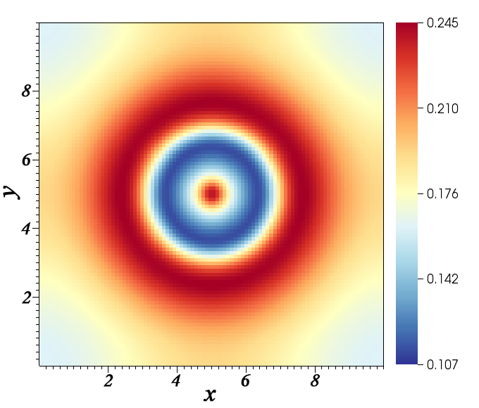
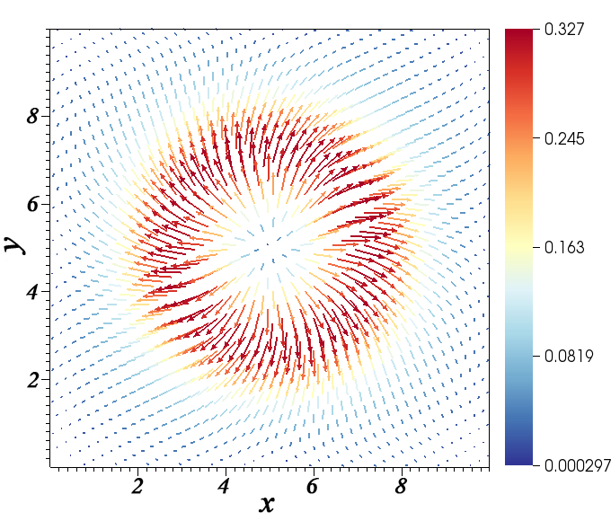
Figure 1: 2D slices show the corrections to the initial guesses when solving Eq. 2 with a relaxation scheme. The initial guesses are given by Eqs. 15 and 16 and the differences between those guesses and the exact solution are shown for field $\Psi$ (left) and $X^{i}$ (right). These also correspond to the fields $u$ and $X^{\prime i}$ as defined in Eq. 29. The choice of parameters for this solution correspond to R3 in Table 1.

In order for $K$ to be a negative constant at the boundaries, corresponding to FLRW-like cosmological expansion, and zero in the center, corresponding to a black hole solution, we also modulate the extrinsic curvature using $W(r)$,

$$K=K_{c}W(r),$$ (17)

where $K_{c}$ is a constant, similar to [8].

By plugging Eq. 17 into the Hamiltonian and momentum constraint equations and taking the approximate solution from Eqs. 15 and 16 to be an initial guess with $J_{k}=(0,0,a)$ in Cartesian coordinates, we can proceed to solve for $\Psi$ and $X^{i}$. The singularities in the solution are avoided by employing the so-called puncture approach; further details regarding this can be found in A. In Fig. 1 we show snapshots of the absolute difference (fields $u$ and $X^{\prime i}$ from Eqs. 29) between the exact solution to Eqs. 2 and the approximate solution of Eqs. Eq. 15 and 16. The main change seen for $\Psi$, which is initially $\mathcal{O}(1)$ at the boundaries and much larger near the black hole as per Eq. 16, is an overall distortion of the physical volume of the spacetime, with additional radial corrections. For $X^{i}$, the predominant correction is a large radial contribution in the transition region.

3 Lattice Evolution

We solve the initial constraints and evolve the spacetime using the grid-based numerical relativity code CosmoGRaPH [26]. We first solve the constraint equations using an integrated elliptical-equation solver, which employs a standard Full Multigrid (FMD) iteration scheme and an inexact-Newton-relaxation method [27]. We verify the resulting initial conditions by checking that the Hamiltonian and momentum constraint equations are satisfied with increasing precision as resolution is increased.

After setting initial conditions, spatial slices are advanced using the BSSNOK formulation of numerical relativity [28, 29, 30], with 4th order Runge-Kutta timestepping. All fields are discretized as cell-centered data, and centered 4th-order finite-difference stencils are used for all derivatives except for advection terms $\sim\beta^{i}\partial_{i}$, where upwind derivatives are used instead. Note that the BSSNOK scheme evolves $\tilde{A}_{ij}=\Psi^{-4}A_{ij}$, rather than the $\hat{A}_{ij}$ defined when setting initial conditions.

The gauge condition used in our simulation is a revised version of the widely employed “1+log” and “Gamma-driver” gauge condition:

$$\partial_{t}\alpha = -2\eta\alpha(K-\langle K\rangle_{\rm edge})+\beta^{i}\partial_{i}\alpha,$$

$$\partial_{t}\beta^{i} = B^{i},$$ (18)

$$\partial_{t}B^{i} = \frac{3}{4}\partial_{t}\Gamma^{i}-B^{i}.$$

This differs from the usual “1+log” gauge by introducing a reference expansion rate, $\langle K\rangle_{\rm edge}$, which is the conformal average of the extrinsic curvature $K$ along all edges of the computational domain box defined in Eq. 26. This gauge choice has been demonstrated to have powerful singularity-avoidance properties[31]; the modification we make by subtracting $K$ relative to the average boundary value allows the spatial slice to be driven towards FLRW-like expansion away from the black hole.

Because of the collapsing nature of the black hole, we have also integrated an Adaptive Mesh Refinement (AMR) framework into the time evolution, provided by the code SAMRAI [32], an open-source structured adaptive-mesh-refinement application infrastructure. By building hierarchies of grid levels with different resolution, dividing and distributing patches into computational nodes, SAMRAI realizes high-efficiency adaptive-mesh refinement and parallelization. To synchronize data on different levels, we use tri-cubic Hermite interpolation[33], which we find results in a high degree of numerical stability.

We also require a technique to locate apparent horizons. Because of the aspherical nature of spinning black holes, there is no symmetry of the apparent horizon that makes it simple to locate. We therefore use the AHFinderDirect package [34] to find the apparent horizon on a given spatial hypersurface. The definition and the method of extracting angular momentum from an isolated horizon come from [35], where the angular momentum of a black hole $J$ is defined as

$$J=\frac{1}{8\pi}\oint(\varphi^{a}R^{b}K_{ab})\mathrm{d}^{2}V.$$ (19)

Note here $R^{b}$ is an outgoing vector normal to the horizon and $\varphi^{a}$ is not a Killing vector of the full spacetime but a symmetry vector defined locally on the horizon that preserves the induced metric $q_{ab}$, so that

$$\mathcal{L}_{\varphi}q_{ab}=0$$ (20)

(see [35] for more detail). The eigenvalue closest to unity associated with the symmetry vector is within a percent of unity, indicating the spacetime is very close to axisymmetric in the vicinity of the black hole.

We then track the black hole’s irreducible mass, spin, and horizon mass, as well as the expansion history of the spacetime. The irreducible and horizon masses are defined as

$$M_{\rm H}^{2} \equiv M_{\rm irr}^{2}+\frac{J^{2}}{4M_{\rm irr}^{2}}$$

$$M_{\rm irr}^{2} \equiv \mathcal{A}/16\pi\,.$$ (21)

Here $\mathcal{A}$ is the area of the horizon, defined as $\mathcal{A}\equiv\oint\sqrt{q}\mathrm{d}^{2}V$, where $q$ is the determinant of the induced metric on the horizon.

In order to examine how well the spinning-black-hole-lattice universe corresponds to a FLRW universe with similar expansion properties, or to check how well the lattice obeys a Friedmann-like equation, we need to define an effective density of the spacetime, $\rho_{\rm eff}$, and an average spacetime expansion rate, $\left<K\right>$. We then define a dimensionless parameter

$$\mathcal{C}\equiv\frac{\rho_{\rm eff}}{\langle K\rangle^{2}/24\pi}\,.$$ (22)

According to the Friedmann equation, one should have $\mathcal{C}=1$ for an appropriately chosen ${\rho_{\rm eff}}$ and $\langle K\rangle$ as the effective Hubble parameter equals $\langle K\rangle/3$.

We first consider whether, in defining ${\rho_{\rm eff}}$ and $\langle K\rangle$, it is more appropriate to use a volume-averaging operation or to average over edges of the box. We can set $\rho_{\rm eff}=\rho_{\rm edge,\,eff}$, given by

$$\rho_{\rm edge,\,eff}\equiv M_{\rm eff}/(D_{\bot}^{2}D_{\parallel}).$$ (23)

$M_{\rm eff}$ can be either $M_{\rm H}$ or $M_{\rm irr}$, while $D_{\bot}$ and $D_{\parallel}$ are distances along edges of the box in directions that are perpendicular and parallel to the spin direction respectively, $D_{i}\equiv\int\mathrm{d}x^{i}\sqrt{\gamma_{ii}}$ for a Cartesian direction $i$ (where no sum over $i$ is implied).

An alternative is to make $\rho_{\rm eff}=\rho_{\rm vol,\,eff}$, with

$$\rho_{\rm vol,\,eff}\equiv M_{\rm eff}/V,$$ (24)

where

$$V\equiv\int_{r>r_{H}}\mathrm{d}^{3}x\sqrt{\gamma}$$ (25)

is the conformal volume exterior to the black-hole horizon.

More generically, we define an averaged physical quantity $Q$ on the edge or volume

$$\left<Q\right>_{\rm edge} \equiv \frac{\sum_{\rm all\;edges}\int\mathrm{d}x^{i}\sqrt{\gamma_{ii}}Q}{\sum_{\rm all\;edges}D_{i}}$$ (26)

$$\left<Q\right>_{\rm vol} \equiv \frac{1}{V}\int_{r>r_{H}}\mathrm{d}^{3}x\sqrt{\gamma}Q\,.$$

We can now define the ratio of the left and right hand sides of the effective Friedmann equations as

$$\mathcal{C}_{\rm edge,\,eff}=\frac{\rho_{\rm edge,\,eff}}{\langle K^{2}\rangle_{\rm edge}/24\pi},\;\;\;\;\;\;\mathcal{C}_{\rm vol,\,eff}=\frac{\rho_{\rm vol,\,eff}}{\langle K^{2}\rangle_{\rm vol}/24\pi}.$$ (27)

4 Results

In this section, we will present our main result. We will mainly focus on the the expansion history and effects of spins. We will also investigate time evolution of dimensionless parameter $\mathcal{C}$ and evaluate the effect of statistics.

4.1 Initial condition effects on physical lattice properties

The free parameters in our setup are the box size $L$, the mass scale $M$, the spin $a$, the extrinsic curvature at the periodic boundary $K_{c}$, and the parameters appearing in the transition function (14), $l$, and $\sigma$. To demonstrate the impact that varying these parameters has on the physical properties of the spacetime (namely the black hole masses, densities, and $\mathcal{C}$), we have listed these properties and the corresponding parameters in Table 1 for ten representative simulations.

Table 1: Parameters of initial setups

Runs	$L$	$a$	$K_{c}$	$l$	$\sigma$	$M_{\rm irr}$	$M_{\rm H}$	$M_{\rm H}/V$	$\mathcal{C}_{{\rm edge},\,H}$	$\mathcal{C}_{{\rm vol},\,H}$	$c$
R1	10	0	-0.21	1	3.5	1.023	1.023	0.000414	0.897	0.829	7.7
R2	10	0.6	-0.21	1	3.5	1.107	1.140	0.000404	0.894	0.817	7.7
R3	10	0.9	-0.21	1	3.5	1.180	1.240	0.000395	0.891	0.807	7.4
R4	10	0	-0.21	0.1	3	0.982	0.982	0.000467	0.996	0.844	8.3
R5	10	0.6	-0.21	0.1	3	1.072	1.108	0.000456	0.994	0.828	7.4
R6	10	0.9	-0.21	0.1	3	1.147	1.212	0.000446	0.993	0.815	8.1
R7	10	0.6	-0.15	1	3.5	1.246	1.269	0.000216	0.900	0.842	7.6
R8	10	0.6	-0.1	1	3.5	1.453	1.468	0.000101	0.904	0.865	7.6
R9	11	0.6	-0.21	1	3.5	1.058	1.096	0.000420	0.921	0.827	7.4
R10	12	0.6	-0.21	1	3.5	1.018	1.060	0.000432	0.941	0.832	7.4

In this table, only the first 2nd-6th columns are free parameters that were chosen initially, while the 7th-11th columns are derived parameters that can only be calculated after initial constraints are fully solved. The $\rho_{\rm eff}$ used in columns for $\mathcal{C}_{{\rm edge},\,H}$ and $\mathcal{C}_{{\rm vol},\,H}$ are calculated using $M_{\rm H}$. The convergence rate for each run on initial slice is represented by parameter $c$ whose definition can be found in Eq. 31. In all runs, we do not vary $M$, instead choosing to work in units where $M=1$.

Examining these initial configurations, we can observe the following:

• Although the input parameter $M$ is equal to $M_{\rm H}$ for a Kerr spacetime with asymptotic flat boundary, the resulting $M_{\rm H}$ in the table only roughly tracks $M$, depending on other parameters as well.

• Both $\mathcal{C}_{{\rm edge},\,H}$ and $\mathcal{C}_{{\rm vol},\,H}$ are somewhat less than 1 initially, and change very little when the spin parameter $a$, box size $L$, or boundary extrinsic curvature $K_{c}$ are varied. This implies that the initial spatial slice is always “close” to FLRW.

• Only by changing the combination of $l$ and $\sigma$ does $\mathcal{C}_{{\rm edge},\,H}$ change significantly; However, the value of $\mathcal{C}_{{\rm vol},\,H}$ still does not change.

• Increasing the box size $L$ (comparing R9 and R10 to R2) does not increase the physical size of the box.

• Changing the boundary extrinsic curvature $K_{c}$ (comparing R7 and R8 to R2) will change the effective density and physical box length significantly, but still keeps the ratio in the last two columns unchanged.

To summarize, the parameters that predominantly determine physical properties of the system are $K_{c}$, $M$, and $a$. These strongly affect the simulation volume and black hole mass and spin. $L$, $l$, and $\sigma$ instead affect the coordinate description of the spacetime, and only weakly affect physical properties.

The initial value of the ratio $\mathcal{C}$ quantifies the deviation from the FLRW universe, and is found to be relatively independent of our parameter choices. We now wish to study its time evolution as well as the best way to fit $\rho_{\rm eff}$ to a FLRW universe. Those topics are our main interests and will be discussed in the following sections.

4.2 Expansion properties and energy content

We can now analyze the different contributions to the Hamiltonian constraint equation, or the different “energy” contributions in the spacetime contributing to expansion. Because we work in a vacuum spacetime, there is no actual stress-energy contribution, and all expansion must be a result of either curvature or kinetic terms in the constraint equations. We can decompose these terms as in Hamilotnian constraint in Eq. 4 to get

$$R/8+\tilde{A}_{ij}\tilde{A}^{ij}/8+K^{2}/12=0,$$ (28)

and analyze the average behavior of: the curvature $\langle R\rangle/8$; the anisotropic expansion term $\langle\tilde{A}_{ij}\tilde{A}^{ij}\rangle/8$, which contains contributions from vector and tensor modes and their interactions; and the expansion itself, $\left<K^{2}\right>/12$.

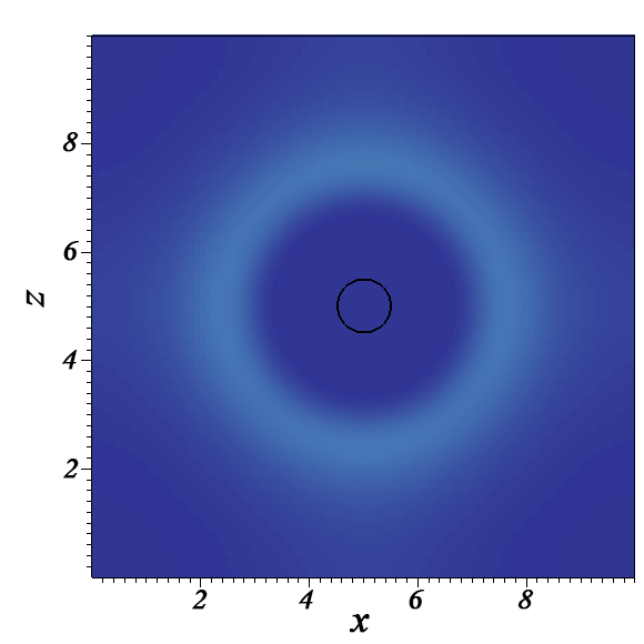
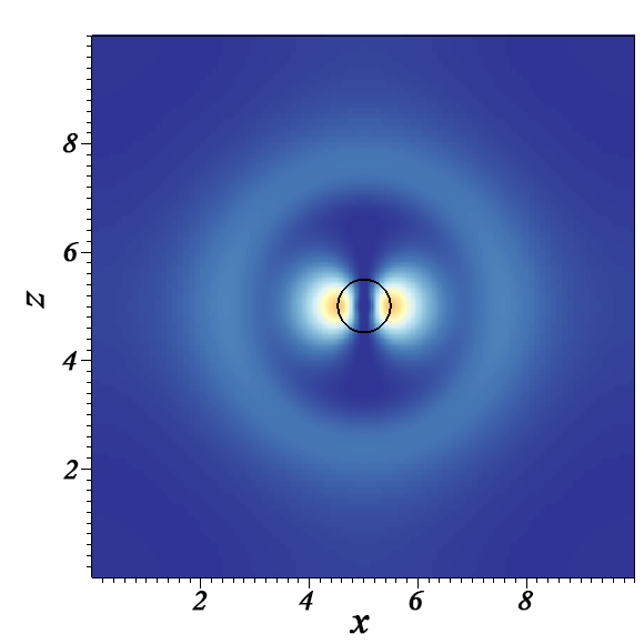
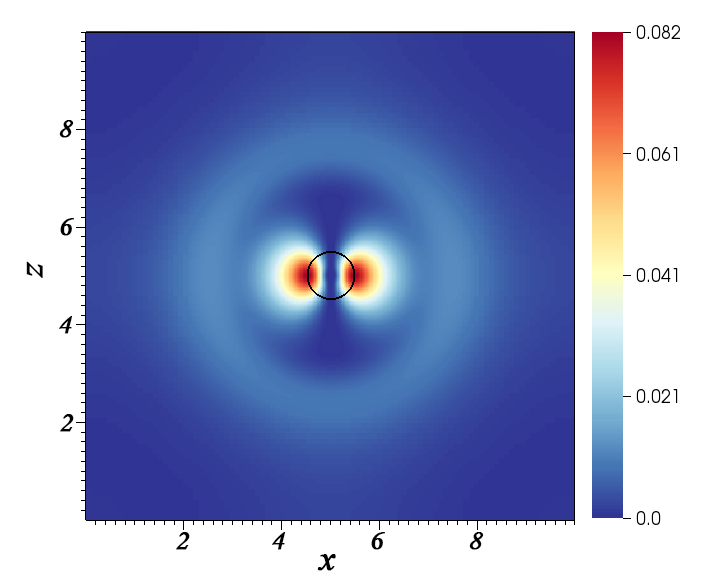
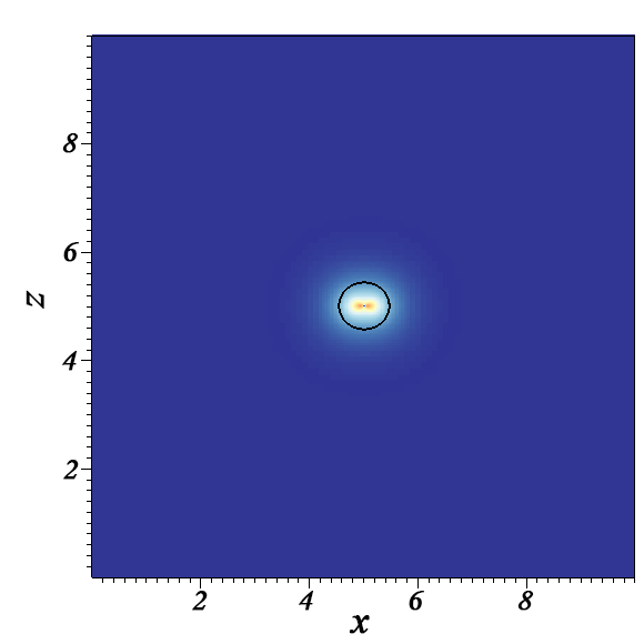
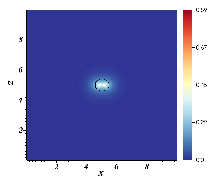
Figure 2: The conformally related trace-free part of the extrinsic curvature, $\tilde{A}_{ij}\tilde{A}^{ij}$, on two-dimensional slices that intersect the black hole through spatial hypersurfaces. The black circles are corresponding slices of apparent horizons. $\tilde{A}_{ij}\tilde{A}^{ij}$ is shown runs R1, R2 and R3 with spins $a=0,0.6,0.9$ (left to right), and at times $t=0,10$ (top to bottom). All quantities are in units where $M=1$.

In Fig. 2, we examine the contribution of the $\tilde{A}_{ij}\tilde{A}^{ij}$ term, which contains information about gravitational-wave and vector-mode energy content. It shows that the vector and tensor modes are concentrated near the black hole horizon, especially as the spacetime evolves and relaxes away from the naïve initial conditions that we set. This is unsurprising in that vector and tensor modes can be sourced nonlinearly in a strong-gravity regime, in contrast to the linear regime in a cosmological setting, where they are expected to be negligible. The absence of this contribution further away from the black hole shows that scalar curvature is the dominant contribution to cosmological expansion.

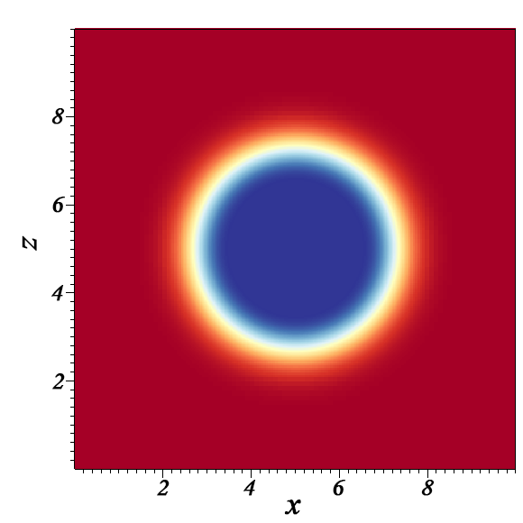
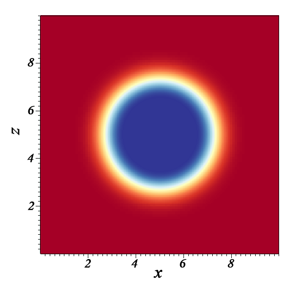
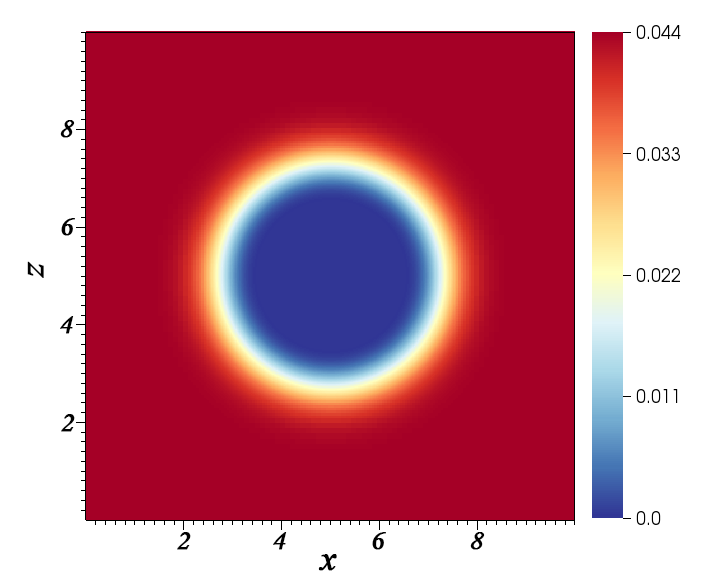
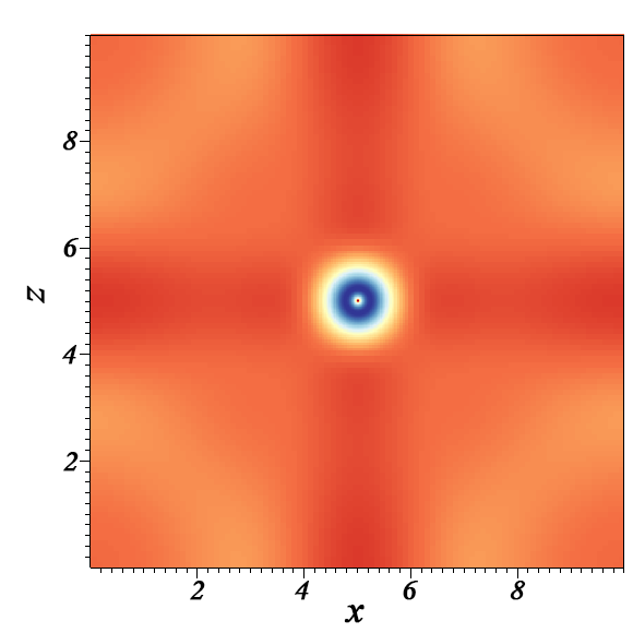
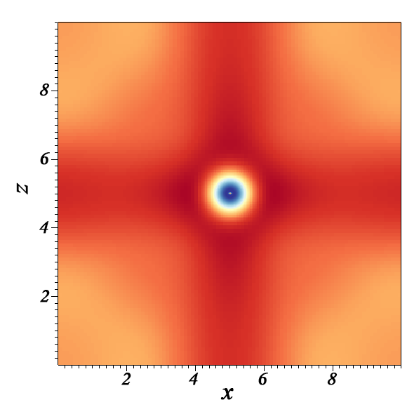
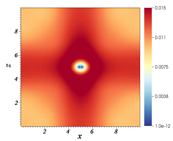
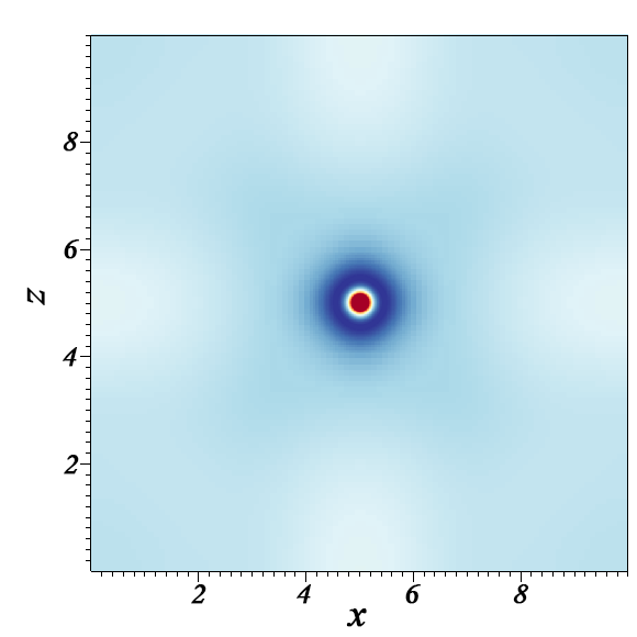
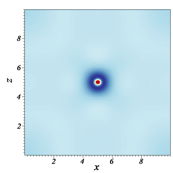
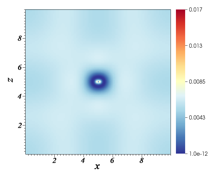
Figure 3: Time evolution snapshots of $K^{2}$ in R1, R2 and R3 with $a=0,0.6,0.9$ (from left to right), and $t=0(M),10(M),15(M)$ (from top to bottom).

Fig. 3 similarly depicts the time evolution of $K^{2}$, which is the volume expansion rate. A behavior very similar to $\tilde{A}_{ij}\tilde{A}^{ij}$ is identified – deviations from cosmological-type expansion are found near the black hole, that gradually become smooth far away from the black hole, especially as the simulation progresses.

Residual oscillations can be seen in the expansion rate, both spatially varying, and as a function of time. The behavior of these oscillations depends on both the initial conditions and the gauge we choose, and we therefore do not consider these to be indicative of an expansion rate that is physically oscillatory, ie. that would strongly impact the way a geodesic observer would view the spacetime. We leave this speculation to future work, although see also [13].

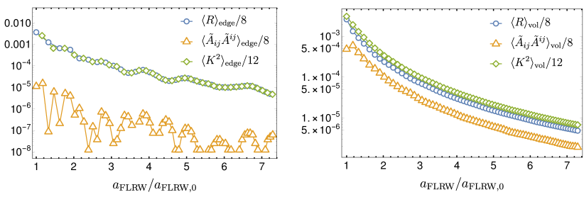
Figure 4: Behavior of the contributions $\left<R\right>/8$, $\langle\tilde{A}_{ij}\tilde{A}^{ij}\rangle/8$ and $\left<K^{2}\right>/12$ to the Hamiltonian constraint in Eq. 28 in R2. The left panel shows edge-averaged terms, and the right panel shows results with volume-averaged terms.

We examine the different contributions to the Hamiltonian constraint equation more quantitatively for R2 in Fig. 4. This demonstrates that the vector and tensor contributions $\langle\tilde{A}_{ij}\tilde{A}^{ij}\rangle$ are relatively small near the edge, but are appreciable when averaged over the volume exterior to the horizon. It is important to note that this interpretation will be affected by gauge choice: for example, the first-order gauge-invariant vector mode usually considered in a cosmological setting, as well as true observables (eg. properties integrated along geodesics according to observers), will contain a contribution from the shift that is not shown here.

4.3 Expansion-mass correspondence

As we evolve the spacetime using the gauge choice of Eq. 3, lengths of edges as well as volume of the spatial slice expand in the intuitively expected manner. The coordinate size of the black hole apparent horizon initially expands as the solution stabilizes, then shrinks due to cosmological expansion, while the area stays the same. We run the code until the black-hole horizon becomes too small to be resolved accurately. At this moment, lengths in spatial slices have roughly grown by a factor of $e^{2}$.

Because of the asymmetric setup, one might expect to see a different expansion rate in different directions. However, we find less than a $0.1\%$ difference in lengths along different edges of the computational box ($D_{\parallel}$ and $D_{\bot}$), and thus will ignore this discrepancy and focus on the quantities averaging on both parallel and perpendicular edges (see Eq. 26).

The masses $M_{\rm irr}$ and $M_{\rm H}$ on the initial slice of each runs are shown in Table 1. During the evolution, their time dependence is nearly negligible: the relative fluctuation in their values is as small as $0.1\%$ and dominated by numerical uncertainty (see B for more detail), consistent with the area theorem and conservation of angular momentum.

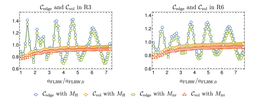
Figure 5: $\mathcal{C}=\rho_{\rm eff}/(\left<K\right>^{2}/24\pi)$ for runs R3 and R6. $\mathcal{C}$ is evaluated using edge and volume averages, with both $M_{\rm irr}$ and $M_{\rm H}$ used in $\rho_{\rm eff}$.

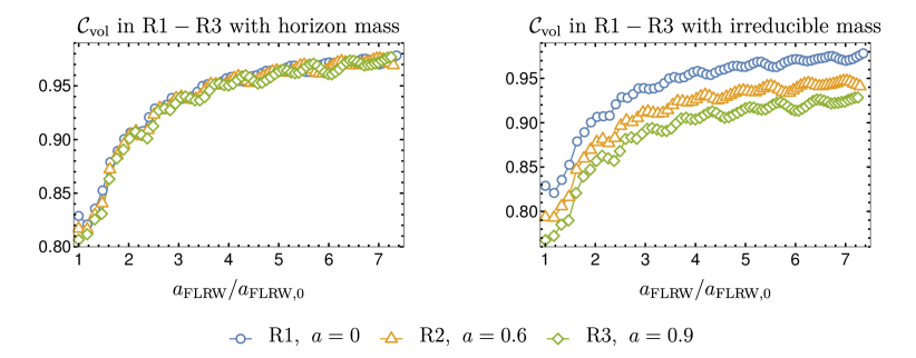
Figure 6: Behavior of the ratio $\mathcal{C}_{\rm vol}$ with different spins and masses. The horizon mass is used in the left panel, while the irreducible mass is used in the right.

From Fig. 5, we can see that $\mathcal{C}_{\rm edge}$ fluctuates with a large amplitude, consistent with behavior seen in [9], while $\mathcal{C}_{\rm vol}$ gently increases to unity. The difference between choices of irreducible mass and horizon mass results in a constant shift between curves, which we investigate below.

We can attempt to reduce the amplitude of oscillations in the edge-averaged case by adjusting $l$ and $\sigma$ to obtain $\mathcal{C}_{\rm edge}\simeq 1$ on the initial slice. Comparing the panels in Fig. 5, we see that this does not help in eliminating the fluctuations. The large amplitude fluctuations we see in $\mathcal{C}_{\rm edge}$ apparently arise from a combination of the way we slice the initial spacetime and the gauge condition, indicating volume-averaged quantities appear to be a more appropriate representation of the physical behavior of the system.

Fig. 6 provides us with more insight into the spin dependence of $\mathcal{C}_{\rm vol}$ for different definitions of mass. $\mathcal{C}_{\rm vol}$ is approximately spin-independent when the horizon mass is used to construct $\rho_{\rm eff}$. It appears to approach the expected matter-dominated FLRW value of unity as the simulation evolves. Neither of these features are maintained when choosing $\rho_{\rm eff}=M_{\rm irr}/V$ (right panel). The diminishing value of $\mathcal{C}_{\rm vol}$ as the spin is increased implies that an energy contribution to the Hamiltonian constraint is not being accounted for. The horizon mass $M_{\rm H}$ is thus a better choice than $M_{\rm irr}$ when considering the effective mass in a spinning-black-hole-lattice universe.

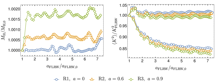
Figure 7: Dependence of $M_{\rm H}/M_{\rm H,0}$ and $\langle K^{2}\rangle_{\rm vol}/\langle K^{2}\rangle_{\rm vol,0}$ as a function of scale factor. We also compare the averaged expansion rate to an FLRW model, according to a best fit function with radiation (top 3 lines) and without (bottom 3 lines), showing the actual expansion is well-described by a mix of matter and radiation.

Lastly, we consider how the averaged values we consider here map to corresponding FLRW spacetimes in Fig. 7. As a function of FLRW scale factor, $a\equiv V^{1/3}$, with V as in Eq. 25, we note that the horizon mass $M_{\rm H}$ is conserved, implying matter-domination-like expansion with $\rho_{\rm eff}\propto a^{-3}_{\rm FLRW}$. There is no spin dependence to within numerical uncertainty. However, the time-dependence of the effective Hubble parameter relative to an FLRW model shows a mix of matter and radiation contributions. The bottom 3 lines in this figure imply that a purely matter dominated expansion $(a/a_{0})^{-3}$ is not a good fit, while the top 3 lines show the behavior is well-described by including radiative content with a best fit function $0.19(a/a_{0})^{-4}+0.81(a/a_{0})^{-3}$.

5 Discussion and Conclusions

In this paper, we have built a new kind of black-hole-lattice universe by solving the constraint equations with a conformal-transverse-traceless decomposition with periodic boundary conditions. A series of space-like hypersurfaces corresponding to expanding universes with spinning black holes were identified. We found that the expansion features of those initial slices were very close to an effective FLRW universe regardless of the initial parameters choices.

We then evolved the initial slices with a singularity-avoiding gauge choice, finding no significant difference between the expansion in directions parallel and perpendicular to the spin. The effective density described by the black hole mass evolved similarly to a matter-dominated universe, ie. the mass of the black hole was conserved, while the effective Hubble parameter only followed matter-dominated behavior at late times. When quantifying the deviation of the expansion rate from FLRW-like behavior, we found that averages taken over edges of the simulation coordinate box displayed large fluctuations, while volume averaged quantities showed much smaller deviations and approached FLRW asymptotically. By fitting the spinning-black-hole-lattice universe to the FLRW universe, we were able to identify the effective mass that governs the expansion as the horizon mass of the black hole, rather than the irreducible mass.

In future work, we can track physical observables through the spacetime, to better characterize the effects of highly non-linear non-stationary perturbations on universes that, like are own, appear to be on-average homogeneous and statistically isotropic on large scales.

It is noteworthy that the spacetimes that we have considered have a preferred direction, determined by the orientation of the spin of the single black hole in the fundamental domain. We anticipate exploring more general initial conditions with multiple spinning black holes and $0$ total angular momentum. Finally, although the spurious gravitational waves introduced by initial gauge fixing (conformally flat and $\hat{A}^{TT}_{ij}=0$) have been shown to not critically affect the late-time evolution in both previous work [25, 36] and in our observation of $\tilde{A}_{ij}\tilde{A}^{ij}$, it may nevertheless be helpful to explore other schemes, like conformal thin-sandwich (CTS) decomposition, to set more general initial conditions with reduced spurious gravitational wave content.

References

Appendix A Using puncture method to build initial data

In a black hole lattice, the metric near the black hole center will be close to an isolated black hole, so we can expect them to have similar divergence properties, i.e., $\Psi$ diverges as $2M/r$ and $X^{i}$ diverges as $ax^{i}/r^{3}$ according to the Bowen-York solution in Eqs. 15 and 16 with $J_{i}=(0,0,a)$.

We therefore employ the puncture approach by defining

$$u \equiv\Psi-\frac{M}{2r}(1-W(r))$$ (29)

$$X^{\prime 1} \equiv X^{1}-\frac{ya(1-W(r))}{r^{3}}$$

$$X^{\prime 2} \equiv X^{2}+\frac{xa(1-W(r))}{r^{3}}$$

$$X^{\prime 3} \equiv X^{3}.$$

By switching from variables $(\Psi,X^{i})$ to $(u,X^{\prime i})$, we expect to replace divergent variables with regular variables and implicitly incorporate the divergence in the solution.

The constraint equations Eq. 2 can then be reduced to

$$\nabla^{2}u-\nabla^{2}\left(\frac{M}{2r}W(r)\right)+\frac{1}{8}\left(\tilde{L}X\right)_{ij}\left(\tilde{L}X\right)^{ij}\Psi^{-7}-\frac{1}{12}K^{2}\Psi^{5}=0$$ (30)

$$\nabla^{2}X^{\prime 1}+\frac{1}{3}\partial^{1}\partial_{j}X^{\prime j}-\nabla^{2}\left(\frac{ya}{r^{3}}W(r)\right)-\frac{2}{3}\Psi^{6}\partial^{1}K=0$$

$$\nabla^{2}X^{\prime 2}+\frac{1}{3}\partial^{2}\partial_{j}X^{\prime j}+\nabla^{2}\left(\frac{xa}{r^{3}}W(r)\right)-\frac{2}{3}\Psi^{6}\partial^{2}K=0$$

$$\nabla^{2}X^{\prime 3}+\frac{1}{3}\partial^{3}\partial_{j}X^{\prime j}-\frac{2}{3}\Psi^{6}\partial^{3}K=0,$$

which contain no divergent terms. We solve for the variables $u$ and $X^{\prime i}$ using a standard multigrid method (more detail can be found in [37]), and the divergent initial data for $\Psi$ and $X^{i}$ can be restored from them.

Appendix B Numerical Convergence Details

We will show here detail of our convergence test. For three runs with different coarsest resolutions, convergence rate is calculated as

$$c\equiv\frac{|f_{N_{c}}-f_{N_{m}}|}{|f_{N_{m}}-f_{N_{f}}|},$$ (31)

where $f_{N_{c}}$, $f_{N_{m}}$ and $f_{N_{f}}$ are values calculated at resolutions $N_{c}$, $N_{m}$ and $N_{f}$, which are from coarsest to finest. Resolutions are chosen to be $64$, $96$ and $128$ respectively in our tests. As among all the simulations in this article the case R3 in Table 1 with spin parameter $a=0.9$ exhibited the most instability, we will only focus on this case.

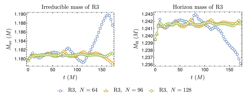
Figure 8: Behavior of irreducible mass (left) and horizon mass (right) with different coarsest resolutions in run R3 with $a=0.9$.

We track the evolution history of both the irreducible mass and the horizon mass at different resolutions in order to check for convergence. These are shown in Fig. 8, and both show small fluctuations that decrease as numerical precision increases. To within this numerical error, the results we find are consistent with the area theorem and with conservation of angular momentum.

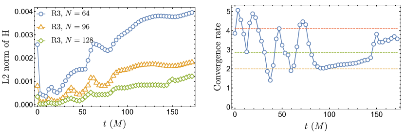
Figure 9: Behavior of the L2 norm of Hamiltonian constraint under different coarsest resolutions and the corresponding convergence rate. Dashed lines in the right plot indicates the 2nd, 3rd, and 4th order of convergence rate correspondingly from bottom to top. Second order of convergence can be achieved.

The L2 norm of the Hamiltonian constraint at different resolutions, as well as the convergence rate, are shown in Fig. 9. Note that the L2 norm of the constraint violation is calculated only outside of the black hole horizon. Second order of convergence rate is achieved, as shown in the figure. Note that during the evolution, AMR hierarchies are built even on the initial slice, the interpolation operations used to build those levels reduce the convergence rate of initial violation from 7 (in the last column of Table 1) to 4. The mismatch between the 2nd order convergence and 4th order stencil mainly results from the truncation error introduced by coarse-fine interfaces.

References

- [1] Planck Collaboration, N. Aghanim et al., “Planck 2018 results. VI. Cosmological parameters,” arXiv:1807.06209 [astro-ph.CO].
- [2] E. Komatsu et al., “Seven-Year Wilkinson Microwave Anisotropy Probe (WMAP) Observations: Cosmological Interpretation,” The Astrophysical Journal Supplement Series 192 (2011) no. 2, 18.
- [3] J. T. Giblin, J. B. Mertens, and G. D. Starkman, “Departures from the Friedmann-Lemaitre-Robertston-Walker Cosmological Model in an Inhomogeneous Universe: A Numerical Examination,” Phys. Rev. Lett. 116 (2016) no. 25, 251301, arXiv:1511.01105 [gr-qc].
- [4] E. Bentivegna and M. Bruni, “Effects of nonlinear inhomogeneity on the cosmic expansion with numerical relativity,” Phys. Rev. Lett. 116 (2016) no. 25, 251302, arXiv:1511.05124 [gr-qc].
- [5] T. Clifton and P. G. Ferreira, “Archipelagian Cosmology: Dynamics and Observables in a Universe with Discretized Matter Content,” Phys. Rev. D80 (2009) 103503, arXiv:0907.4109 [astro-ph.CO]. [Erratum: Phys. Rev.D84,109902(2011)].
- [6] C.-M. Yoo, H. Abe, K.-i. Nakao, and Y. Takamori, “Black Hole Universe: Construction and Analysis of Initial Data,” Phys. Rev. D86 (2012) 044027, arXiv:1204.2411 [gr-qc].
- [7] E. Bentivegna and M. Korzynski, “Evolution of a periodic eight-black-hole lattice in numerical relativity,” Class. Quant. Grav. 29 (2012) 165007, arXiv:1204.3568 [gr-qc].
- [8] C.-M. Yoo, H. Okawa, and K.-i. Nakao, “Black Hole Universe: Time Evolution,” Phys. Rev. Lett. 111 (2013) 161102, arXiv:1306.1389 [gr-qc].
- [9] E. Bentivegna and M. Korzynski, “Evolution of a family of expanding cubic black-hole lattices in numerical relativity,” Class. Quant. Grav. 30 (2013) 235008, arXiv:1306.4055 [gr-qc].
- [10] E. Bentivegna, “Black-hole lattices,” Springer Proc. Math. Stat. 60 (2014) 143–146, arXiv:1307.7673 [gr-qc].
- [11] T. Clifton, D. Gregoris, K. Rosquist, and R. Tavakol, “Exact Evolution of Discrete Relativistic Cosmological Models,” JCAP 1311 (2013) 010, arXiv:1309.2876 [gr-qc].
- [12] C.-M. Yoo and H. Okawa, “Black hole universe with a cosmological constant,” Phys. Rev. D89 (2014) no. 12, 123502, arXiv:1404.1435 [gr-qc].
- [13] E. Bentivegna, T. Clifton, J. Durk, M. Korzyński, and K. Rosquist, “Black-Hole Lattices as Cosmological Models,” Class. Quant. Grav. 35 (2018) no. 17, 175004, arXiv:1801.01083 [gr-qc].
- [14] E. Bentivegna, M. Korzyński, I. Hinder, and D. Gerlicher, “Light propagation through black-hole lattices,” JCAP 1703 (2017) no. 03, 014, arXiv:1611.09275 [gr-qc].
- [15] V. A. A. Sanghai, P. Fleury, and T. Clifton, “Ray tracing and Hubble diagrams in post-Newtonian cosmology,” JCAP 1707 (2017) no. 07, 028, arXiv:1705.02328 [astro-ph.CO].
- [16] P. Fleury, J. Larena, and J.-P. Uzan, “Weak gravitational lensing of finite beams,” Phys. Rev. Lett. 119 (2017) no. 19, 191101, arXiv:1706.09383 [gr-qc].
- [17] M. Korzyński, “Backreaction and continuum limit in a closed universe filled with black holes,” Class. Quant. Grav. 31 (2014) 085002, arXiv:1312.0494 [gr-qc].
- [18] M. Korzyński, “Nonlinear effects of general relativity from multiscale structure,” Class. Quant. Grav. 32 (2015) no. 21, 215013, arXiv:1412.3865 [gr-qc].
- [19] P. Fleury, J. Larena, and J.-P. Uzan, “Cosmic convergence and shear with extended sources,” Phys. Rev. D99 (2019) no. 2, 023525, arXiv:1809.03919 [astro-ph.CO].
- [20] J. Durk and T. Clifton, “A Quasi-Static Approach to Structure Formation in Black Hole Universes,” JCAP 1710 (2017) no. 10, 012, arXiv:1707.08056 [gr-qc].
- [21] T. Clifton, K. Rosquist, and R. Tavakol, “An Exact quantification of backreaction in relativistic cosmology,” Phys. Rev. D86 (2012) 043506, arXiv:1203.6478 [gr-qc].
- [22] T. Clifton, “The Method of Images in Cosmology,” Class. Quant. Grav. 31 (2014) 175010, arXiv:1405.3197 [gr-qc].
- [23] J. W. York, Jr., “Kinematics and Dynamics of General Relativity,” in Sources of Gravitational Radiation: Proceedings of the Battelle Seattle Workshop, pp. 83–126. 1978.
- [24] J. M. Bowen and J. W. York, Jr., “Time asymmetric initial data for black holes and black hole collisions,” Phys. Rev. D21 (1980) 2047–2056.
- [25] R. J. Gleiser, C. O. Nicasio, R. H. Price, and J. Pullin, “Evolving the Bowen-York initial data for spinning black holes,” Phys. Rev. D57 (1998) 3401–3407, arXiv:gr-qc/9710096 [gr-qc].
- [26] J. B. Mertens, J. T. Giblin, and G. D. Starkman, “Integration of inhomogeneous cosmological spacetimes in the BSSN formalism,” Phys. Rev. D93 (2016) no. 12, 124059, arXiv:1511.01106 [gr-qc].
- [27] W. H. Press, S. A. Teukolsky, W. T. Vetterling, and B. P. Flannery, Numerical Recipes 3rd Edition: The Art of Scientific Computing. Cambridge University Press, New York, NY, USA, 3 ed., 2007.
- [28] T. Nakamura, K. Oohara, and Y. Kojima, “General Relativistic Collapse to Black Holes and Gravitational Waves from Black Holes,” Prog. Theor. Phys. Suppl. 90 (1987) 1–218.
- [29] M. Shibata and T. Nakamura, “Evolution of three-dimensional gravitational waves: Harmonic slicing case,” Phys. Rev. D52 (1995) 5428–5444.
- [30] T. W. Baumgarte and S. L. Shapiro, “On the numerical integration of Einstein’s field equations,” Phys. Rev. D59 (1998) 024007, arXiv:gr-qc/9810065 [gr-qc].
- [31] J. D. Brown, O. Sarbach, E. Schnetter, M. Tiglio, P. Diener, I. Hawke, and D. Pollney, “Excision without excision: The Relativistic turducken,” Phys. Rev. D76 (2007) 081503, arXiv:0707.3101 [gr-qc].
- [32] A. M. Wissink, R. D. Hornung, S. R. Kohn, S. S. Smith, and N. Elliott, “Large scale parallel structured AMR calculations using the SAMRAI framework,” in Proceedings of the 2001 ACM/IEEE conference on Supercomputing, Denver, CO, USA, November 10-16, 2001, CD-ROM, p. 6. 2001. http://doi.acm.org/10.1145/582034.582040.
- [33] E. Kreyszig, Advanced Engineering Mathematics. John Wiley & Sons, 2019.
- [34] J. Thornburg, “A Fast apparent horizon finder for three-dimensional Cartesian grids in numerical relativity,” Class. Quant. Grav. 21 (2004) 743–766, arXiv:gr-qc/0306056 [gr-qc].
- [35] O. Dreyer, B. Krishnan, D. Shoemaker, and E. Schnetter, “Introduction to isolated horizons in numerical relativity,” Phys. Rev. D67 (2003) 024018, arXiv:gr-qc/0206008 [gr-qc].
- [36] L. M. Burko, T. W. Baumgarte, and C. Beetle, “Towards a novel wave-extraction method for numerical relativity: III. Analytical examples for the Beetle-Burko radiation scalar,” Phys. Rev. D73 (2006) 024002, arXiv:gr-qc/0505028 [gr-qc].
- [37] W. H. Press, S. A. Teukolsky, W. T. Vettering, and B. P. Flannery, “Numerical Recipes in C++: The Art of Scientific Computing (2nd edn),” European Journal of Physics 24 (2003) no. 3, .