Evolution of cosmic ray electron spectra in magnetohydrodynamical simulations

Abstract

Cosmic ray (CR) electrons reveal key insights into the non-thermal physics of the interstellar medium (ISM), galaxies, galaxy clusters, and active galactic nuclei by means of their inverse Compton $\gamma$-ray emission and synchrotron emission in magnetic fields. While magnetohydrodynamical (MHD) simulations with CR protons capture their dynamical impact on these systems, only few computational studies include CR electron physics because of the short cooling time-scales and complex hysteresis effects, which require a numerically expensive, high-resolution spectral treatment. Since CR electrons produce important non-thermal observational signatures, such a spectral CR electron treatment is important to link MHD simulations to observations. We present an efficient post-processing code for Cosmic Ray Electron Spectra that are evolved in Time (crest) on Lagrangian tracer particles. The CR electron spectra are very accurately evolved on comparably large MHD time steps owing to an innovative hybrid numerical-analytical scheme. crest is coupled to the cosmological MHD code arepo and treats all important aspects of spectral CR electron evolution such as adiabatic expansion and compression, Coulomb losses, radiative losses in form of inverse Compton, bremsstrahlung and synchrotron processes, diffusive shock acceleration and reacceleration, Fermi-II reacceleration, and secondary electron injection. After showing various code validations of idealized one-zone simulations, we study the coupling of crest to MHD simulations. We demonstrate that the CR electron spectra are efficiently and accurately evolved in shock-tube and Sedov–Taylor blast wave simulations. This opens up the possibility to produce self-consistent synthetic observables of non-thermal emission processes in various astrophysical environments.

1 Introduction

CRs are ubiquitous in many astrophysical environments, such as the ISM, galaxies, galaxy clusters and active galactic nuclei (AGN). CRs are non-thermal, charged particles consisting of a hadronic component (mainly protons and alpha particles) as well as leptons (mainly electrons and positrons). The leptonic component (henceforth referred to as CR electrons) suffers fast radiative losses via synchrotron interactions with magnetic fields and inverse Compton (IC) interactions with ambient photon fields. Hence they are directly linked to observations of the non-thermal emission from radio to gamma-ray wavelengths. Hadronic CRs (henceforth referred to as CR protons) are interesting since they play an important dynamical role in the ISM due to their energy equipartition with turbulent and magnetic energy in the midplane of the Milky Way (Boulares & Cox, 1990). As CR protons stream and diffuse vertically from their sources in the galactic midplane, their emerging CR proton pressure gradient can dominate the force balance and accelerate the gas, thus driving a galactic outflow as shown in one-dimensional (1D) magnetic flux-tube models (Breitschwerdt et al., 1991; Zirakashvili et al., 1996; Ptuskin et al., 1997; Everett et al., 2008; Samui et al., 2018) and three-dimensional (3D) simulations (Uhlig et al., 2012; Booth et al., 2013; Salem & Bryan, 2014; Pakmor et al., 2016c; Simpson et al., 2016; Girichidis et al., 2016; Pfrommer et al., 2017b; Ruszkowski et al., 2017a; Jacob et al., 2018).

Fast-streaming CR protons resonantly excite Alfvén waves through the “streaming instability” (Kulsrud & Pearce, 1969). Damping of these waves effectively transfers CR to thermal energy. This process is thought to provide the physical heating mechanism underlying the “cooling flow problem” in galaxy clusters where the cooling gas and nuclear activity appear to be tightly coupled to a self-regulated feedback loop (McNamara & Nulsen, 2007). As CR protons stream out of AGN lobes they can stably heat the surrounding cooling intracluster medium (Loewenstein et al., 1991; Guo & Oh, 2008; Enßlin et al., 2011; Fujita & Ohira, 2012; Pfrommer, 2013; Jacob & Pfrommer, 2017a, b; Ruszkowski et al., 2017b; Ehlert et al., 2018).

Early studies of CR protons in computational cosmology were performed by the Eulerian mesh cosmocr code (Miniati, 2001) and at cosmological shocks by N-body/hydrodynamical simulations (Ryu et al., 2003). The first MHD simulations with active CR proton transport were performed with the zeus-3d code (Hanasz & Lesch, 2003). Modeling CR proton physics in the smoothed particle hydrodynamics code gadget-2 enabled adaptive spatial resolution in high-density environments and to explore the impact of CR protons on the formation of galaxies and galaxy clusters (Pfrommer et al., 2006; Enßlin et al., 2007; Jubelgas et al., 2008). Further numerical CR proton studies were performed with the Eulerian mesh code piernik (Hanasz et al., 2010), the adaptive mesh refinement codes ramses (Booth et al., 2013; Dubois & Commerçon, 2016), enzo (Salem & Bryan, 2014), flash (Girichidis et al., 2016, 2018), and pluto (Mignone et al., 2018), the moving-mesh code arepo (Pakmor et al., 2016b; Pfrommer et al., 2017a).

In comparison to CR protons, the energy of CR electrons falls short by a factor of about 100 at the solar radius in the Milky Way (Zweibel, 2013); hence CR electrons are not dynamically important. The cooling time-scale of relativistic CR electrons with Lorentz factors $\gamma\gtrsim 10^{3}$ is much shorter than that of relativistic CR protons at the same energy per particle. While CR protons can only effectively cool via rare hadronic interactions (thereby lowering the resulting luminosity), CR electrons cool efficiently via synchrotron and IC interactions. This means that much of the non-thermal physics is only observationally accessible through the leptonic emission channel. Thus, it is very important to model the momentum spectrum of CR electrons alongside (magneto)hydrodynamical simulations in order to produce realistic synthetic non-thermal observables. Comparing those to observational data enables scrutinising our simulated physics and our understanding of galaxy formation, evolution of galaxy clusters or AGN jet physics.

Supernova remnants (SNRs) provide us with important insights into the physics of particle acceleration and have been observed from radio to $\gamma$-ray energies (Helder et al., 2012; Blasi, 2013; Bykov et al., 2018). This radiation is produced by hadronic and leptonic processes, and the ambient density and the magnetic field strength of the SNR determine which of these processes dominates. In low-density environments of SNR, such as RX J1713.7-3946, IC emission by CR electrons likely dominates the $\gamma$-ray emission (Ellison et al. 2012, but see Celli et al. 2019, for an interpretation in terms of hadronic emission). Stellar bow shocks of massive runaway stars are also a site of particle acceleration, e.g. the radio emission observed in the bow shock of the runaway star BD +$43^{\circ}3654$ might be produced by synchrotron radiation of CR electrons (Benaglia et al., 2010).

Many galaxies exhibit galactic outflows that shine in radio, X-rays, and $\gamma$-rays. Understanding the physics of galactic outflows is the holy grail of galaxy formation. The most prominent example of these outflows are the Fermi bubbles, which extend to about $8\text{\,}\mathrm{k}\mathrm{p}\mathrm{c}$ north and south from the central region of our Milky Way. They are observed as hard-spectrum gamma-ray structures (Su et al., 2010; Dobler et al., 2010) which coincide with radio lobes (Carretti et al., 2013). The origin of the Fermi bubbles remains elusive and it is not clear whether hadronic CR proton interactions or leptonic IC emission scenarios are dominant for the observed $\gamma$-ray emission. Models generally rely on AGN or starburst events. There are several attempts to simulate the evolution of the Fermi bubbles (Yang & Ruszkowski, 2017; Mertsch & Petrosian, 2019) or more generally, to understand radio signatures of outflows in external galaxies (Heesen et al., 2016). However, self-consistent (magneto)hydrodynamical simulations of the Milky Way with CR proton and electron physics are still missing.

Galaxy clusters shine in radio due to synchrotron emission of CR electrons in turbulent cluster magnetic fields. There are three important classes of radio sources in galaxy clusters: radio relics, giant haloes and radio mini haloes (Bykov et al., 2019). Giant radio haloes are characterised by spatially extended regions of diffuse, unpolarised radio emission with an irregular morphology that is centred on the cluster. In contrast, radio relics are often located at the periphery of clusters and show a high degree of polarization with an irregular, elongated morphology. There are several simulation studies of CR electron acceleration and diffuse radio synchrotron emission in the context of galaxy clusters (e.g. Miniati et al., 2001; Miniati, 2003; Pfrommer et al., 2008; Battaglia et al., 2009; Pinzke et al., 2013, 2017; Vazza et al., 2012; Donnert et al., 2013; Donnert & Brunetti, 2014; Guo et al., 2014a, b; Kang et al., 2019).

The plethora of astrophysical systems that shine through leptonic non-thermal radiation makes it inevitable to evolve the CR proton and electron physics on top of MHD simulations in order to distinguish hadronic and leptonic scenarios. Despite the importance of CR electrons, there are only few numerical codes that can evolve the spectra of CR electrons in MHD simulations, e.g. the pluto code with CR electrons on Lagrangian particles (Vaidya et al., 2018). We aim at further closing this gap by presenting a numerical post-processing code for Cosmic Ray Electron Spectra that are evolved in Time (crest), which works together with (magneto)hydrodynamical codes that have Lagrangian tracer particles. In this work, we present the algorithm and test its implementation in one-zone problems. To evolve the CR electron spectrum spatially and temporally resolved alongside MHD simulations, we couple crest to the massively-parallel hydrodynamical code arepo (Springel, 2010), that can also follow CR proton physics (Pfrommer et al., 2017a). In evolving the CR electron spectrum, crest includes adiabatic effects, all important energy loss processes of CR electron as well as energy gain processes such as diffusive shock acceleration (via the Fermi-I process) and reacceleration, Fermi-II reacceleration via particle interactions with compressible turbulence, and secondary electron injection.

We present the physical and numerical foundations of our algorithm in section 2. We proceed with numerical tests of our code, including idealized one-zone tests in section 3 and simulations with arepo in section 4. We conclude in section 5 and provide an outlook of future astrophysical applications of our work. In appendix A, we detail the discretisation scheme and numerical algorithms adopted for solving the Fokker–Planck equation of CR electrons. We use the cgs system of units throughout this work.

2 Methodology

Here, we introduce the theoretical background before we explain our discretisation scheme and numerical algorithms to describe our subgrid scale model for Fermi-I acceleration. We then present analytical solutions of limiting cases and our hybrid algorithm that combines analytical and numerical solutions to the transport equation of CR electrons.

2.1 Theoretical background

2.1.1 Transport equation

The CR electron distribution is completely described by the phase space density $f({\bf\it x},{\bf\it p},t)$ whose evolution is given by the relativistic Vlasov equation. Throughout this paper, we use the dimensionless electron momentum, ${\bf\it p}={\bf\it P}/(m_{\mathrm{e}}c)$. CR electrons gyrate around magnetic field lines which are subject to random fluctuations. The application of quasi-linear theory by ensemble averaging over fluctuations, and the use of the diffusion approximation, i.e. the assumption of near-isotropic equilibrium as a consequence of frequent pitch-angle scattering on MHD turbulence leads to the Fokker–Planck equation (Schlickeiser, 1989a; Zank, 2014).

We follow the transport of CR electrons on Lagrangian tracer particles and include continuous losses plus a source term (Schlickeiser, 1989b). Here, we assume that CR electrons are transported with the gas as they are confined to their gyration orbits around turbulent magnetic fields, which are frozen into the moving plasma. The Fokker–Planck equation for the 1D distribution in momentum space is related to the 3D distribution via $f(p)=4\pi p^{2}f^{\mathrm{3D}}(p)$ and obeys the Fokker–Planck equation without CR streaming (e.g. Pinzke et al., 2017)

$$\derivative{f(p,t)}{t}=\begin{aligned} &\phantom{{}+{}}\partialderivative{p}\left[f(p,t)\frac{p}{3}\left(\divergence{{\bf\it\varv}}\right)\right]-\left(\divergence{{\bf\it\varv}}\right)f(p,t)\\ &-\partialderivative{p}\left[f(p,t)\dot{p}(p,t)\right]+Q(p,t)\\ &-\partialderivative{p}\left[\frac{f(p,t)}{p^{2}}\partialderivative{p}(p^{2}D_{\!p\!p})\right]+\partialderivative[2]{p}\left[D_{\!p\!p}f(p,t)\right]\\ &+\boldsymbol{\nabla}\boldsymbol{\cdot}\left[\textbf{{K}}\boldsymbol{\cdot}\boldsymbol{\nabla}f(p,t)\right],\end{aligned}$$ (1)

where $\derivative*{t}=\partial/\partial t+\boldsymbol{\varv\cdot\nabla}$ is the Lagrangian time derivative and $p=\absolutevalue{{\bf\it p}}$ is the absolute value of the momentum. The first line on the right-hand side describes adiabatic changes resulting from changes in the gas velocity ${\bf\it\varv}$ and Fermi-I acceleration and reacceleration (in combination with spatial diffusion, see Blandford & Eichler, 1987).

The second line describes energy losses (i.e. Coulomb and radiative losses) $\dot{p}(p,t)$ and injection with source function $Q(p,t)$ for unresolved subgrid acceleration processes and secondary electron injection that are produced in hadronic interactions of CR protons with the ambient gas. The latter process is described by $Q_{\mathrm{inj}}=\dot{C}_{\mathrm{inj}}p^{-\alpha_{\mathrm{inj}}}$ with injection slope $\alpha_{\mathrm{inj}}$ that is identical to that of the CR proton distribution, an injection rate $\dot{C}_{\mathrm{inj}}=C_{\mathrm{inj}}/\tau_{\mathrm{pp}}$, where $C_{\mathrm{inj}}\propto n_{\mathrm{crp}}$ and $\tau_{\mathrm{pp}}=1/(c\sigma_{\mathrm{pp}}n_{\mathrm{tar}})$ (Mannheim & Schlickeiser, 1994). Here, $c$ is the speed of light, $\sigma_{\mathrm{pp}}$ is the proton-proton cross-section, $n_{\mathrm{tar}}$ is the target proton density, and $n_{\mathrm{crp}}$ is the number density of CR protons, which we dynamically evolve with the CR proton module of arepo (Pfrommer et al., 2017a).

The third line represents the momentum diffusion (Fermi-II reacceleration) with a momentum-dependent diffusion $D_{\!p\!p}(p)$ while the last line describes spatial CR diffusion with the diffusion tensor K. Because we do not resolve the necessary scales and plasma processes to directly follow diffusive shock acceleration via the adiabatic and diffusive terms, we have to treat Fermi-I acceleration and reacceleration in form of an analytic subgrid model via the source term $Q(p,t)$ in our code. We defer the explicit treatment of spatial CR diffusion, as well as CR streaming, to future studies.

2.1.2 Loss processes

We note that energy losses are in general time dependent as photon fields, magnetic fields and electron number densities change in time. We will suppress the explicit time dependence in the following formulae for simplicity. Coulomb losses (Gould, 1972) are described by

$$\dot{p}_{\mathrm{c}}(p)=-\frac{3\sigma_{\mathrm{T}}n_{\mathrm{e}}c}{2\beta^{2}}\begin{aligned} &\left[\ln(\frac{m_{\mathrm{e}}c^{2}\beta\sqrt{\gamma-1}}{\hbar\omega_{\mathrm{pl}}})\vphantom{\left(\frac{\gamma-1}{4\gamma}\right)^{2}}\right.\\ &\left.\ +\ln(2)\left(\frac{\beta^{2}}{2}+\frac{1}{\gamma}\right)+\frac{1}{2}+\left(\frac{\gamma-1}{4\gamma}\right)^{2}\vphantom{\ln(\frac{m_{\mathrm{e}}c^{2}\beta\sqrt{\gamma-1}}{\hbar\omega_{\mathrm{pl}}})}\right],\end{aligned}$$ (2)

where $\sigma_{\mathrm{T}}=8\pi e^{4}(m_{\mathrm{e}}c^{2})^{-2}/3$ is the Thomson cross-section, $\hbar$ is the reduced Planck constant, $m_{\mathrm{e}}$ the electron mass, $\beta=p(1+p^{2})^{-1/2}$ is the dimensionless CR electron velocity, and $\gamma=(1+p^{2})^{1/2}$ is the Lorentz factor of CR electrons. The electron density is $n_{\mathrm{e}}=n_{\mathrm{gas}}X_{\mathrm{H}}x_{\mathrm{e}}$ where $X_{\mathrm{H}}$ is the hydrogen mass fraction and $x_{\mathrm{e}}=n_{\mathrm{e}}/n_{\mathrm{H}}$ is the ionization fraction, the ratio of electron density-to-hydrogen density, which is denoted by $n_{\mathrm{H}}$. The plasma frequency is $\omega_{\mathrm{pl}}=\sqrt{4\pi e^{2}n_{\mathrm{e}}/m_{\mathrm{e}}}$ and $e$ denotes the elementary charge.

Charged particles experience synchrotron losses in magnetic fields and experience inverse Compton scattering off of photon fields (Rybicki & Lightman, 1986). Synchrotron losses are given by

$$\dot{p}_{\mathrm{s}}(p)=-\frac{4\sigma_{\mathrm{T}}p^{2}}{3m_{\mathrm{e}}c\beta}\frac{B^{2}}{8\pi},$$ (3)

and inverse Compton processes by

$$\dot{p}_{\mathrm{ic}}(p)=-\frac{4\sigma_{\mathrm{T}}p^{2}}{3m_{\mathrm{e}}c\beta}\varepsilon_{\mathrm{ph}},$$ (4)

where the total radiation field is a sum over the cosmic microwave background (CMB) radiation and star light, $\varepsilon_{\mathrm{ph}}=\varepsilon_{\mathrm{star}}+\varepsilon_{\mathrm{cmb}}$. The momentum loss rate of the bremsstrahlung loss process is given by

$$\dot{p}_{\mathrm{b}}(p)=-\frac{16}{3}\alpha\left(\frac{e^{2}}{m_{\mathrm{e}}^{2}c^{3}}\right)^{2}\gamma\chi\left[E(p)\right],$$ (5)

where $\alpha$ is the fine-structure constant and the function $\chi\left[E(p)\right]$ is provided by Koch & Motz (1959). The total energy loss rate is given by the sum of all losses:

$$\dot{p}(p,t)=\dot{p}_{\mathrm{c}}(p)+\dot{p}_{\mathrm{s}}(p)+\dot{p}_{\mathrm{ic}}(p)+\dot{p}_{\mathrm{b}}(p).$$ (6)

2.1.3 Fermi-I acceleration and reacceleration

Diffusive shock acceleration also known as Fermi-I acceleration is an important energy gain process for CR electrons. It is a combination of direct acceleration of electrons from the thermal pool and of reacceleration of a fossil electron distribution $f_{\mathrm{pre}}$ in the pre-shock region, if present.

The total spectrum in the post-shock region is obtained by evaluating adiabatic changes and spatial diffusion of equation (1) at the shock. The analytic solution of the total post-shock spectrum is (Bell, 1978; Drury, 1983; Blandford & Eichler, 1987)

$$f_{\mathrm{post}}(p)=f_{\mathrm{reac}}(p)+f_{\mathrm{acc}}(p),$$ (7)

where the reaccelerated and accelerated spectrum are

$$f_{\mathrm{reac}}(p) =(\alpha_{\mathrm{acc}}+2)p^{-\alpha_{\mathrm{acc}}}\int_{p_{\mathrm{inj}}}^{p}p^{\prime\alpha_{\mathrm{acc}}-1}f_{\mathrm{pre}}(p^{\prime})\differential{p^{\prime}}\mbox{ and}$$ (8)

$$f_{\mathrm{acc}}(p) =C_{\mathrm{acc}}p^{-\alpha_{\mathrm{acc}}}\Theta(p-p_{\mathrm{inj}}),$$ (9)

respectively, where $C_{\mathrm{acc}}$ is the normalization and $p_{\mathrm{inj}}$ is the injection momentum of the accelerated spectrum. The spectral index $\alpha_{\mathrm{acc}}$ is calculated by

$$\alpha_{\mathrm{acc}}=\frac{r+2}{r-1},$$ (10)

where $r=\rho_{\mathrm{post}}/\rho_{\mathrm{pre}}$ denotes the shock compression ratio, i.e. the ratio of post-shock to pre-shock gas density. We also take cooling processes into account, which lead to a modified spectrum with a momentum cutoff (Enßlin et al., 1998; Zirakashvili & Aharonian, 2007; Pinzke & Pfrommer, 2010) of the form

$$\tilde{f}_{\mathrm{post}}(p)=f_{\mathrm{post}}(p)\left[1+a\left(\frac{p}{p_{\mathrm{acc}}}\right)^{b}\right]^{c}\exp[-\left(\frac{p}{p_{\mathrm{acc}}}\right)^{2}],$$ (11)

where we adopt the parameters $a=0.66$, $b=2.5$, and $c=1.8$ and $p_{\mathrm{acc}}$ is the cutoff momentum of the (re)accelerated spectrum

$$p_{\mathrm{acc}}=\begin{aligned} &\frac{\varv_{\mathrm{post}}}{c}\sqrt{\frac{3e(r-1)}{4\sigma_{\mathrm{T}}}}\\ &\times\left[\frac{B_{\mathrm{pre}}^{2}/(8\pi)+\varepsilon_{\mathrm{ph}}}{rB_{\mathrm{pre}}}+\frac{B_{\mathrm{post}}^{2}/(8\pi)+\varepsilon_{\mathrm{ph}}}{B_{\mathrm{post}}}\right]^{-1/2},\end{aligned}$$ (12)

where $\varv_{\mathrm{post}}$ is the post-shock velocity in the shock rest frame and $B_{\mathrm{pre}}$ and $B_{\mathrm{post}}$ are the pre- and post-shock magnetic fields. Here, we assume a parallel shock geometry so that the magnetic field strength is constant across the shock. We postpone a modelling of the dependencies of the maximum electron energy on magnetic obliquity and amplified magnetic fields via plasma effects such as the non-resonant hybrid instability driven by the CR proton current propagating upstream of the shock (Bell, 2004).

2.1.4 Fermi-II reacceleration

Stochastic acceleration, originally proposed by Fermi (1949), describes the energy gains of CRs through random collisions with plasma waves and turbulence. As the gain per collision process is of second order in the velocity ratio of collision counterpart to particle, it is also referred to as Fermi-II reacceleration (Petrosian, 2012). However, Coulomb cooling is too fast for stochastic acceleration from the thermal pool to be efficient in cluster and galactic environments (Petrosian, 2001). Therefore, the Fermi-II process is only efficient in reaccelerating a fossil non-thermal electron distribution.

Fermi-II reacceleration by turbulent magnetic fields was investigated in galaxy clusters as primary energy source for diffusive radio emission from CR electrons in the Coma cluster (Jaffe, 1977; Schlickeiser et al., 1987). There are different energy transfer channels of turbulent energy injection into CR, e.g. via magnetosonic waves (Ptuskin, 1988) or via transit time damping (TTD) of compressible fast magnetosonic modes (Brunetti & Lazarian, 2007, 2011).

CRs gain energy in turbulent reacceleration through transit time damping. The momentum diffusion in equation (1) is given by

$$D_{\!p\!p}=D_{0}p^{2}$$ (13)

where the physics of turbulent reacceleration is encapsulated in the constant $D_{0}$ (Pinzke et al., 2017). The momentum diffusion time is $\tau_{\!p\!p}=p^{2}/(4D_{\!p\!p})$ which is $\tau_{\!p\!p}=1/(4D_{0})$ according to equation (13).

2.2 Numerical discretisation

2.2.1 General setup

In order to solve equation (1) numerically, we apply three discretisations to the CR electron phase space density $f=f({\bf\it x},p,t)$. (i) We discretise $f$ in configuration space with Lagrangian tracer particles, (ii) we discretise the momentum spectrum of every tracer particle with piecewise constant values per momentum bin, and (iii) $f$ is discretised in time. The momentum grid is equally spaced in logarithmic space and we use $N$ bins between the lowest momentum $p_{\mathrm{min}}$ and highest momentum $p_{\mathrm{max}}$. The bin centres are located at

$$p_{i}=p_{\mathrm{min}}\exp[\left(i+\frac{1}{2}\right)\Delta\ln p] \mbox{for }i=0,1,\ldots,N-1,$$ (14)

and the bin edges are given by

$$p_{i-\frac{1}{2}}=p_{\mathrm{min}}\exp(i\,\Delta\ln p) \mbox{for }i=0,1,\ldots,N,$$ (15)

where $\Delta\ln p=\ln(p_{\mathrm{max}}/p_{\mathrm{min}})/N$ is the grid spacing. The spectrum is defined on all bin centers and is evolved in time from $t$ by a time step $\Delta t$ with an operator split approach,

$$f({\bf\it x},p,t+\Delta t)=\mathcal{A}_{\mathrm{diff}}\left(\frac{\Delta t}{2}\right)\mathcal{A}_{\mathrm{adv}}\left(\Delta t\right)\mathcal{A}_{\mathrm{diff}}\left(\frac{\Delta t}{2}\right)f({\bf\it x},p,t).$$ (16)

Adiabatic changes, Fermi-I (re)acceleration, cooling, and injection are calculated with an advection operator $\mathcal{A}_{\mathrm{adv}}$ and diffusion in momentum space is calculated with a diffusion operator $\mathcal{A}_{\mathrm{diff}}$ that both advance the solution for the time step of their arguments.

The advection operator is based on a flux-conserving finite volume scheme with a second-order piecewise linear reconstruction of the spectrum. The terms $\partialderivative*{p}\left\{f(p)[p(\divergence{{\bf\it\varv}})/3-\dot{p}]\right\}$, which include cooling and partially adiabatic changes, are interpreted as advection in momentum space in order to calculate fluxes across the bin edges given in equation (15). In addition, we use the non-linear van Leer flux limiter (van Leer, 1977). The remaining terms for injection, Fermi-I (re)acceleration and adiabatic changes, are treated as an inhomogeneity of the partial differential equation (for details, see appendix A.1). Our implementation is second-order accurate in time and momentum space.

The diffusion operator is based on a finite difference scheme with a semi-implicit Crank–Nicolson algorithm, which is accurate to second order in time and to first order in momentum space (for details, see appendix A.2).

2.2.2 Time steps and characteristic momenta

The overall time step $\Delta t$ in equation (16) is determined by

$$\Delta t=\min\mathopen{}\left(\Delta t_{\mathrm{adv}},\Delta t_{\mathrm{diff}}\right),$$ (17)

the minimum of the time step for advection and diffusion,

$$\Delta t_{\mathrm{adv}}=C_{\mathrm{CFL}}\left[\max\mathopen{}\left(\frac{\absolutevalue{\dot{p}(p)}}{\Delta p}\right)+\frac{\absolutevalue{\Delta n}}{n}\right]^{-1}\mbox{ and}$$ (18)

$$\Delta t_{\mathrm{diff}}=C_{\mathrm{CFL}}\left[\max\mathopen{}\left(\frac{D_{\!p\!p}(p)}{p^{2}}\right)\right]^{-1},$$ (19)

respectively, where $\Delta n$ is the density change of the background gas and the parameter $C_{\mathrm{CFL}}$ is the Courant–Friedrichs–Lewy number for which we use $C_{\mathrm{CFL}}=0.7$ in our simulations. In principle, the maxima in equations (18) and (19) have to be evaluated for all momentum bins, i.e. for $i\in\left[0,\,N{-}1\right]$. However, in the absence of Fermi-I (re)acceleration, the momentum range of the advection and diffusion operator decreases due to rapidly cooling of the spectrum at low and high momenta. We therefore cut the spectrum at $f_{\mathrm{cut}}$ below which we treat numerical values of the spectrum as zero. Hence, there is a low- and a high-momentum cutoff

$$p_{\mathrm{lcut}}=\min\mathopen{}\left(\left\{p:f(p)\geq f_{\mathrm{cut}}\right\}\right)\mbox{ and}$$ (20)

$$p_{\mathrm{hcut}}=\max\mathopen{}\left(\left\{p:f(p)\geq f_{\mathrm{cut}}\right\}\right),$$ (21)

respectively, and the related indices of the momentum bins

$$i_{\mathrm{lcut}}=\max\mathopen{}\left[0,\min\mathopen{}\left(\left\{i:p_{i}<p_{\mathrm{lcut}}\right\}\right)-2\right]\mbox{and}$$ (22)

$$i_{\mathrm{hcut}}=\min\mathopen{}\left[N,\max\mathopen{}\left(\left\{i:p_{i}>p_{\mathrm{lcut}}\right\}\right)+3\right]$$ (23)

in between which the maxima in equations (18) and (19) have to be evaluated, i.e. for $i\in\left[i_{\mathrm{lcut}},\,i_{\mathrm{hcut}}{-}1\right]$. We consider two extra bins in equations (22) and (23) due to the ghost cells of the advection operator. The cutoff momenta and the related indices are calculated after every time step.

For clarity, we provide a synopsis of all important momenta and related bin indices:

• $p_{\mathrm{min}}$ and $p_{\mathrm{max}}$ are the minimum and maximum momenta of our momentum grid, respectively. The corresponding indices are $i_{\mathrm{min}}=0$ and $i_{\mathrm{max}}=N{-}1$.

• $p_{\mathrm{lcut}}$ ($p_{\mathrm{hcut}}$) describes the momentum below (above) which the spectrum is treated as zero. The corresponding indices $i_{\mathrm{lcut}}$ and $i_{\mathrm{hcut}}$ account for the ghost cells of the advection operator and are given in equations (22) and (23).

• $p_{\mathrm{low}}$ and $p_{\mathrm{high}}$ denote the transition momenta between the numerical and the analytical solution for the low- and high-momentum regime, respectively. The definition is given in section 2.3.6.

• $p_{\mathrm{cool}}$ is the momentum related to inverse Compton and synchrotron cooling in the analytical solution. In the case of freely cooling it coincides with the high-momentum cooling cutoff. In the case of Fermi-I (re)acceleration and injection it is the transition momentum from a source dominated to a steady-state spectrum (see section 2.3.3).

• $p_{\mathrm{acc}}$ is the maximum momentum of Fermi-I (re)acceleration where spatial diffusion and cooling balance each other.

• $p_{\mathrm{inj}}$ is the injection momentum of Fermi-I (re)acceleration where the non-thermal spectrum is transitions to the non-thermal spectrum.

2.2.3 Modelling Fermi-I (re)acceleration

We develop an algorithm to account for the Fermi-I process on our tracer particles and aim at reconstructing the discontinuous Rankine–Hugoniot jump conditions on the Lagrangian particle trajectories with the aid of a shock finder in a hydrodynamical scheme. To this end, we use the adaptive moving-mesh code arepo (Springel, 2010) with CR protons (Pfrommer et al., 2017a) and employ the shock finder by Schaal & Springel (2015), which detects cells in the pre-shock region, the shock surface, and the post-shock zone. The shock direction is determined by the normalized negative gradient

$$\textbf{{n}}_{s}=-\frac{\boldsymbol{\nabla}\tilde{T}}{\absolutevalue{\boldsymbol{\nabla}\tilde{T}}}$$ (24)

of the pseudo temperature which is given by

$$k\tilde{T}=\frac{\mu m_{\mathrm{p}}(P_{\mathrm{th}}+P_{\mathrm{crp}})}{\rho},$$ (25)

where $\mu$ is the mean molecular weight, $m_{\mathrm{p}}$ is the proton mass, $\rho$ is the gas mass density, and $P_{\mathrm{th}}$ and $P_{\mathrm{crp}}$ denote the thermal and CR proton pressure, respectively. Cells of the shock zone are identified by (i) converging flows, i.e. they have a negative velocity divergence, while (ii) spurious shocks are filtered out and (iii) the algorithm applies a safeguard in the form of a lower limit to the temperature and density jump (from pre- to post-shock quantities) to prevent false-positive detections of numerical noise. The shock surface cell is identified with the cell in the shock zone that shows a maximally converging flow along the shock direction. Pre- and post-shock quantities are obtained from the first cells outside the shock zone in the direction of shock propagation and opposite to it, respectively. The algorithm determines the Mach number $\mathcal{M}$ by the pressure jump and calculates a fraction $\zeta_{\mathrm{e}}(\theta)$ of the shock-dissipated energy $E_{\mathrm{diss}}$ that is converted into the acceleration of CR electrons,

$$\Delta E_{\mathrm{cre}}=\zeta_{\mathrm{e}}(\theta)E_{\mathrm{diss}}.$$ (26)

Here, $\theta$ is the upstream magnetic obliquity, which is the angle between the direction of shock propagation and the magnetic field. In this paper, we assume an acceleration efficiency of $\zeta_{\mathrm{e}}=10^{-3}$. This corresponds to a ratio of accelerated CR electron to proton energies of $\Delta E_{\mathrm{cre}}/\Delta E_{\mathrm{crp}}=10^{-2}$ for efficient CR proton acceleration (Pfrommer et al., 2017a). We defer a discussion of the obliquity dependent acceleration of CR electrons to future studies. We point out that our description is flexible and can be easily adapted to include new particle-in-cell simulation results on the shock acceleration of CR electrons (e.g. Guo et al., 2014a, b; Park et al., 2015).

As soon as the tracer particle reaches a shock zone cell, we keep the background density fixed in order to prevent adiabatic heating before encountering the shock. When the tracer particle transitions from the shock zone to the shock surface cell, we first calculate the reaccelerated spectrum if there is any fossil spectrum and secondly, the directly accelerated spectrum. The ambient density of the tracer particles is then set to the post-shock gas density. In order to model reacceleration and direct acceleration, we assume continuous injection as a subgrid model and adopt the source functions

$$Q_{\mathrm{reac}}(p) =\frac{f_{\mathrm{reac}}(p)}{\Delta t}\mbox{ and}$$ (27)

$$Q_{\mathrm{acc}}(p) =\frac{C_{\mathrm{acc}}}{\Delta t}p^{-\alpha_{\mathrm{acc}}}\Theta(p-p_{\mathrm{inj}}),$$ (28)

where $\Delta t$ is the the time difference between two MHD time steps.

As described above, the efficiency of direct Fermi-I acceleration depends on the total dissipated energy at the shock, which is numerically broadened to a few cells in finite-volume codes such as arepo. By contrast, Fermi-I reacceleration only depends on the amplitude of the fossil electron distribution in the pre-shock region (see equation 8), which is known at the shock surface cell. In both cases, the slope is solely determined by the Mach number.

To model direct acceleration, we calculate and apply the source function for acceleration of equation (28) for every time step during which the tracer particle resides in a shock surface or in the post-shock cells for the numerical reasons given above. By contract, the source function for reacceleration (equation 27) is only applied during one MHD time step after the tracer particle has encountered the shock surface cell.

We calculate $\alpha_{\mathrm{acc}}$ from the density jump at the shock, $r~{}=~{}\rho_{\mathrm{post}}/\rho_{\mathrm{pre}}$, where the pre-shock density communicated to the shock cell via the arepo shock finder, and the post-shock density is obtained via

$$\rho_{\mathrm{post}}=\rho_{\mathrm{pre}}\frac{(\gamma_{\mathrm{eff}}+1)\mathcal{M}^{2}}{(\gamma_{\mathrm{eff}}-1)\mathcal{M}^{2}+2},$$ (29)

where the effective adiabatic index is given by

$$\gamma_{\mathrm{eff}}=\frac{\gamma_{\mathrm{crp}}P_{\mathrm{crp}}+\gamma_{\mathrm{th}}P_{\mathrm{th}}}{P_{\mathrm{crp}}+P_{\mathrm{th}}}$$ (30)

with $\gamma_{\mathrm{th}}=5/3$ for gas and $\gamma_{\mathrm{crp}}=4/3$ for CR protons.

In order to determine the energy of the freshly accelerated CR electrons, we demand its energy density to be a fixed fraction of the freshly accelerated CR proton energy density at the shock. In practice, we attach the accelerated spectrum to the thermal Maxwellian,

$$f_{\mathrm{th}}(p)=4\pi n_{\mathrm{e,th}}\left(\frac{m_{\mathrm{e}}c^{2}}{2\pi k_{\mathrm{B}}T}\right)^{3/2}p^{2}\exp(-\frac{m_{\mathrm{e}}c^{2}p^{2}}{2k_{\mathrm{B}}T})$$ (31)

at the injection momentum $p_{\mathrm{inj}}$ which determines the normalization

$$C_{\mathrm{acc}}=f_{\mathrm{th}}(p_{\mathrm{inj}})p_{\mathrm{inj}}^{\alpha_{\mathrm{acc}}}.$$ (32)

We use this normalization and the energy of accelerated CR electrons $\Delta E_{\mathrm{cre}}$, see equation (26), to determine the injection momentum by the condition

$$\int_{0}^{\infty}f_{\mathrm{th}}(p_{\mathrm{inj}})p^{\alpha_{\mathrm{acc}}}_{\mathrm{inj}}p^{-\alpha_{\mathrm{acc}}}\Theta(p-p_{\mathrm{inj}})E_{\mathrm{e,kin}}(p)\mathrm{d}p=\frac{\Delta E_{\mathrm{cre}}}{V_{\mathrm{cell}}},$$ (33)

where $E_{\mathrm{e,kin}}(p)=\left[\sqrt{1+p^{2}}-1\right]m_{\mathrm{e}}c^{2}$ is the kinetic energy and $V_{\mathrm{cell}}$ is the volume of the arepo cell, in which the particle resides.

2.3 Analytical solutions

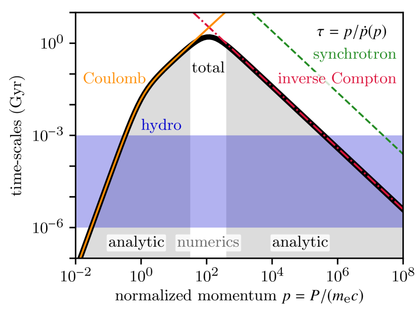
Figure 1: Characteristic time-scales for electron cooling ($n_{\mathrm{gas}}=${10}^{-3}\text{\,}{\mathrm{cm}}^{-3}$$, $B=$5\text{\,}\mathrm{\SIUnitSymbolMicro G}$$, $\varepsilon_{\mathrm{ph}}=6\varepsilon_{\mathrm{cmb}}$, $z=0$) and typical hydrodynamical time steps adopted in simulations of the ISM and galaxy formation (blue band). The grey area shows the ranges where either Coulomb or inverse Compton plus synchrotron cooling dominate and where analytical solutions can be used. Transition momenta of numerical and analytical solutions are $p_{\mathrm{low}}=$3\text{\times}{10}^{1}$$ and $p_{\mathrm{high}}=$4\text{\times}{10}^{2}$$.

The time-scale of all electron cooling processes decreases for low and for high momenta as can be seen in Figure 1, where we show the cooling times as a function of momentum. Hence, for very low momenta and very high the cooling time-scales become smaller than the typical time step of an MHD simulation. In order to have an efficient calculation of the CR electron spectrum, which advances on time steps similar to the MHD time step, we use analytical solutions for low and high momenta together with the fully numerical treatment for intermediate momenta. We call the combination of both treatments semi-analytical solution.

2.3.1 General solutions

We follow the derivations described by Sarazin (1999) which we summarise here. The starting point for the analytical solution of the cooling term in equation (1) is the momentum loss of an individual electron. Its momentum is shifted from the initial momentum $p_{\mathrm{ini}}$ to the momentum $p$ during a time interval of $\Delta t$

$$\int_{p_{\mathrm{ini}}}^{p}\frac{1}{\dot{p}(p^{\prime})}\differential{p^{\prime}}=\Delta t.$$ (34)

Equation (34) is solved for the initial momentum $p_{\mathrm{ini}}(p,\Delta t)$, which is used in the analytical solution of the cooled spectrum

$$f(p,t_{0}+\Delta t)=f(p_{\mathrm{ini}}(p,\Delta t),t_{0})\frac{\dot{p}(p_{\mathrm{ini}}(p,\Delta t),t_{0}+\Delta t)}{\dot{p}(p,t_{0})}.$$ (35)

The cooled spectrum can be interpreted as a momentum shift of the initial spectrum at time $t_{0}$ multiplied with a momentum-dependent cooling factor. If there is no initial spectrum at $t_{0}$ and if the source function $Q(p,t)$ is constant and continuous in time, the spectrum after time $t$ is self-similar:

$$f_{\mathrm{self}}(p,t)=f_{\mathrm{steady}}(p)-f_{\mathrm{steady}}(p_{\mathrm{ini}}(p,t))\frac{\dot{p}(p_{\mathrm{ini}}(p,t))}{\dot{p}(p)},$$ (36)

where we use the steady-state solution

$$f_{\mathrm{steady}}(p)=\frac{1}{|\dot{p}(p)|}\int_{p}^{\infty}Q(p)\differential{p}.$$ (37)

This means that the self-similar solution is derived by subtracting the cooled steady-state solution from the original steady-state solution. The self-similar spectrum consists of three characteristic momentum ranges, i.e. low, intermediate, and high momenta. For low and high momenta, where the cooling times are smaller than the current time step, the spectrum is already in steady state. In the intermediate momentum range, the spectrum is dominated by the source spectrum as we show later.

The analytical solutions of the cooled spectrum in equation (35) and of the self-similar spectrum in equation (36) need a functional representation of the spectrum at time $t_{0}$ for the entire momentum range. As the spectrum is calculated on a discrete momentum grid with piecewise constant values, we calculate an interpolation function at every time with the Steffen’s method (Steffen, 1990), which is cubic and monotonic between neighbouring discrete momenta. This interpolation function is used to calculate the analytic solution after a time step $\Delta t$.

In the following, we present the analytical solutions for both low and high momenta. We use a source function $Q(p)=\dot{C}_{\mathrm{acc}}\,p^{-\alpha_{\mathrm{acc}}}$ for the self-similar solution of acceleration and cooling. We note that we have $\dot{C}_{\mathrm{acc}}=C_{\mathrm{acc}}/\Delta t$ for our discretisation and that a source function for injection by hadronic processes with $Q(p)=\dot{C}_{\mathrm{inj}}\,p^{-\alpha_{\mathrm{inj}}}$ gives similar results for the self-similar solution. Note that the self-similar solution is not used in our code (see also section 2.3.5) but in order to compare simulation results to their analytic solutions.

2.3.2 Solution for low momenta

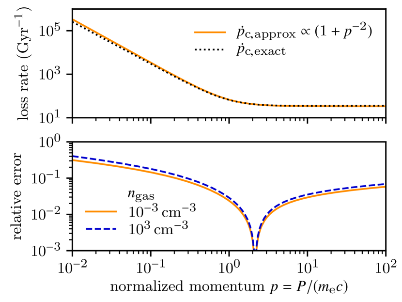
Figure 2: Comparison between exact and approximate formulae for Coulomb losses (equations (2) and (38)). The top panel shows the loss rates for a gas of density $1\text{\times}{10}^{-3}\text{\,}{\mathrm{cm}}^{-3}$ and the bottom panel shows the relative error of the approximate formula for two different gas densities.

Coulomb losses are dominating at small momenta. The analytical solution requires calculating the integral in equation (34) and solving for the initial momentum $p_{\mathrm{ini}}(p,\Delta t)$. In general, this cannot be done in closed analytic form for the exact Coulomb loss rate given in equation (2). We therefore use an approximation (Pinzke et al., 2013)

$$\dot{p}_{\mathrm{c}}(p)=b_{\mathrm{c}}\left(1+p^{-2}\right)\mbox{ with }b_{\mathrm{c}}=\frac{-3\sigma_{\mathrm{T}}n_{\mathrm{e}}c}{2}\ln(\frac{m_{\mathrm{e}}c^{2}}{\hbar\omega_{\mathrm{pl}}}),$$ (38)

which is accurate to $<30\%$ for momenta $10^{-2}\leq p\leq 10^{2}$ as can be seen in Figure 2. The integral for the momentum shift in equation (34) evaluated with the approximate form of the Coulomb loss rate is

$$\int\frac{1}{\dot{p}_{\mathrm{c}}(p)}\differential{p}=\frac{1}{-b_{\mathrm{c}}}\left[p-\arctan(p)\right]\approx\frac{1}{-b_{\mathrm{c}}}\left(\frac{p^{3}}{3+p^{2}}\right),$$ (39)

where we used a Padé approximation (Brezinski, 1996) in the last step. The momentum shift due to Coulomb cooling is then given by

$$p_{\mathrm{ini}}(p,\Delta t)=\frac{1}{3}\begin{aligned} &\left[a+\left(a^{3}+\frac{9}{2}\sqrt{4a^{4}+81a^{2}}+\frac{81a}{2}\right)^{1/3}\right.\\ &\left.~{}+a^{2}\left(a^{3}+\frac{9}{2}\sqrt{4a^{4}+81a^{2}}+\frac{81a}{2}\right)^{-1/3}\right],\end{aligned}$$ (40)

with $a=p^{3}\Big{/}\left(3+p^{2}\right)-b_{\mathrm{c}}\Delta t$. The analytical solution for the cooled spectrum (see equation (35)) is given by

$$f(p,\Delta t)=f[p_{\mathrm{ini}}(p,\Delta t),0]\frac{1+\left[p_{\mathrm{ini}}(p,\Delta t)\right]^{-2}}{1+p^{-2}}.$$ (41)

The self-similar spectrum is given by

$$\begin{aligned} &f_{\mathrm{self}}(p,\Delta t)\\ &=\frac{\dot{C}_{\mathrm{acc}}}{(1-\alpha_{\mathrm{acc}})}\begin{aligned} &\left\{\frac{p^{-\alpha_{\mathrm{acc}}+1}}{\dot{p}_{\mathrm{c}}^{\phantom{2}}(p)}\right.\\ &\left.\phantom{\Bigg{\{}}-\frac{\left[p_{\mathrm{ini}}(p,\Delta t)\right]^{-\alpha_{\mathrm{acc}}+1}}{\dot{p}_{\mathrm{c}}[p_{\mathrm{ini}}(p,\Delta t)]}\frac{1+\left[p_{\mathrm{ini}}(p,\Delta t)\right]^{-2}}{1+p^{-2}}\right\}\end{aligned}\end{aligned}$$ (42)

where we use the exact Coulomb loss rate for the first term in the bracket in order to satisfy $f_{\mathrm{self}}\rightarrow f_{\mathrm{steady}}$ for $\Delta t\rightarrow\infty$.

2.3.3 Solution for high momenta

For large momenta, inverse Compton and synchrotron cooling are dominating and both loss rates have the same momentum scaling. We define for convenience the sum of both as

$$\dot{p}_{\mathrm{ic+s}}(p)=\dot{p}_{\mathrm{ic}}(p)+\dot{p}_{\mathrm{s}}(p)=p^{2}b_{\mathrm{ic+s}}$$ (43)

where $b_{\mathrm{ic+s}}=-4\sigma_{\mathrm{T}}\left(B^{2}/8\pi+\varepsilon_{\mathrm{ph}}\right)/(3m_{\mathrm{e}}c\beta)$ denotes the momentum independent factor of both loss rates. The momentum shift during a time interval $\Delta t$ according to equation (34) is

$$p_{\mathrm{ini}}(p,\Delta t)=\frac{p}{1-p/p_{\mathrm{cool}}(\Delta t)}$$ (44)

where $p_{\mathrm{cool}}(\Delta t)=\left(-b_{\mathrm{ic+s}}\Delta t\right)^{-1}$ is the cooling cutoff of IC and synchrotron losses. In the following, we omit the explicit time dependence of $p_{\mathrm{cool}}(\Delta t)$. The analytical solution of the cooled spectrum (see equation (35)) is given by

$$f(p,\Delta t)=\left\{\begin{aligned} &f\mathopen{}\left(\frac{p}{1-p/p_{\mathrm{cool}}},0\right)\left(1-\frac{p}{p_{\mathrm{cool}}}\right)^{-2},&&p<p_{\mathrm{cool}}\\ &0,&&p\geq p_{\mathrm{cool}}\end{aligned}\right.$$ (45)

and the solution of the self-similar spectrum (see equation (36)) is

$$f_{\mathrm{self}}(p,\Delta t)=\frac{\dot{C}_{\mathrm{acc}}p^{-(\alpha_{\mathrm{acc}}+1)}}{b_{\mathrm{ic+s}}(1-\alpha_{\mathrm{acc}})}\left\{\begin{aligned} &\left(1-\frac{p}{p_{\mathrm{cool}}}\right)^{\alpha_{\mathrm{acc}}-1},&&p<p_{\mathrm{cool}},\\ &1,&&p\geq p_{\mathrm{cool}}.\end{aligned}\right.$$ (46)

2.3.4 Adiabatic changes and cooling

Pure adiabatic changes due to expansion or compression of the background gas leave the phase space density of the CR electrons invariant (Enßlin et al., 2007). An initial spectrum of the form

$$f_{\mathrm{ini}}(p)=Cp^{-\alpha}\Theta(p-q)$$ (47)

with normalisation $C$, slope $\alpha$ and low-momentum cutoff $q$ transforms into

$$f(p)=C{}^{(\alpha+2)/3}p^{-\alpha} \Theta\Bigl{(}p-{}^{1/3}q\Bigr{)}$$ (48)

due to an adiabatic change of the background density from $n_{\mathrm{ini}}$ to $n$ and $\ratio=n/n_{\mathrm{ini}}$ denotes the the ratio of final-to-initial density. Similar to the analytical description for cooling processes, this evolution can be interpreted as a shift in momentum space from an initial momentum $p_{\mathrm{ini}}$ to momentum $p$ by $p_{\mathrm{ini}}(p,x)=p{}^{-1/3}$ and an overall scaling with the factor ^2/3

$$f(p,\ratio)={}^{2/3}f_{\mathrm{ini}}\Bigl{(}p{}^{-1/3}\Bigr{)}.$$ (49)

Our code adopts this equation in combination with the analytical description of radiation and Coulomb cooling processes. The evolution of the CR electron spectrum during small time intervals $\Delta t$ and for small density ratios $\ratio=n(t+\Delta t)/n(t)$ is described by

$$f(p,t+\Delta t)={}^{2/3}f\mathopen{}\left[p_{\mathrm{ini}}\mathopen{}\left(\frac{p}{{}^{1/3}},\Delta t\right),t\right]\frac{\dot{p}\mathopen{}\left[p_{\mathrm{ini}}\mathopen{}\left(p{}^{-1/3},\Delta t\right)\right]}{\dot{p}\mathopen{}\left(p{}^{-1/3}\right)},$$ (50)

where $p_{\mathrm{ini}}(p,\Delta t)$ denotes the momentum shift due to cooling as given in equation (40) for low momenta and in equation (44) for high momenta.

2.3.5 Injection, Fermi-I (re)acceleration and cooling

The analytic solution for the case of cooling and CR electron injection, by hadronic interactions or by our subgrid model of Fermi-I acceleration and reacceleration, is in principle given by the self-similar solution in equation (36) at time $t$. However, we cannot use the self-similar solution because (i) injection and (re)acceleration source function and cooling rates are generally time-dependent, (ii) we need to evolve the previously existing spectrum, and (iii) we evolve the spectrum on differential time steps $\Delta t$ from time $t_{n}$ to $t_{n+1}$. For large momenta with $p/\dot{p}_{\mathrm{ic+s}}(p)<\Delta t$, we use the analytic steady-state solution. For the remaining momentum range, we use an operator-split method. First, we calculate injection and Fermi-I (re)acceleration during a half time step

$$f\mathopen{}\left(p,t_{n}+\frac{\Delta t}{2}\right)=f(p,t_{n})+\frac{\Delta t}{2}Q(p).$$ (51)

We then calculate the effect of cooling and adiabatic changes on $f(p,t_{n}+{\Delta t}/2)$ during a full time step. Finally, we account for injection and (re)acceleration during another half time step to obtain the spectrum at time $t_{n+1}$,

$$f(p,t_{n+1})=\begin{aligned} &f\mathopen{}\left[p_{\mathrm{ini}}\mathopen{}\left(\frac{p}{{}^{1/3}},\Delta t\right),t+\frac{\Delta t}{2}\right]\frac{\dot{p}\mathopen{}\left[p_{\mathrm{ini}}\mathopen{}\left(p{}^{-1/3},\Delta t\right)\right]}{{}^{-2/3}\dot{p}\mathopen{}\left(p{}^{-1/3}\right)}\\ &+\frac{\Delta t}{2}Q(p).\end{aligned}$$ (52)

2.3.6 Combining analytical and numerical solutions

In general, the momentum loss rate $\dot{p}(p)$ is the sum of all loss processes which complicates the integral in equation (34) and the analytical solution for $p_{\mathrm{ini}}(p,\Delta t)$. As we have seen in the preceding subsections, analytical solutions are possible for both low momenta where Coulomb losses are dominating and for high momenta where inverse Compton and synchrotron losses are dominating. Our code determines the transition momenta of the numerical and analytical solutions,

$$p_{\mathrm{low}}=\max\mathopen{}\left(\{p:\tau_{\mathrm{c}}(p)<\epsilon\tau_{\mathrm{b+ic+s}}(p)\ \land\ \tau_{\mathrm{c}}(p)\leq\tau_{\mathrm{hyd}}\}\right)\mbox{ and}$$ (53)

$$p_{\mathrm{high}}=\min\mathopen{}\left(\{p:\tau_{\mathrm{ic+s}}(p)<\epsilon\tau_{\mathrm{b+c}}(p)\ \land\ \tau_{\mathrm{ic+s}}(p)\leq\tau_{\mathrm{hyd}}\}\right)$$ (54)

for low and high momenta, respectively. We also take the constraints due to the hydrodynamical time-scale $\tau_{\mathrm{hyd}}$ into account. The characteristic cooling time-scales are $\tau_{\mathrm{c}}=p/\dot{p}_{\mathrm{c}}(p)$ for Coulomb losses, $\tau_{\mathrm{b}}=p/\dot{p}_{\mathrm{b}}(p)$ for bremsstrahlung, and $\tau_{\mathrm{ic+s}}=p/\dot{p}_{\mathrm{ic+s}}(p)$ for IC and synchrotron cooling. The transition momentum is determined by a free parameter, which we set to $\epsilon=0.1$. The characteristic cooling time-scales and the transition momenta are displayed in Figure 1.

We determine corresponding indices of the transition momentum bins as

$$i_{\mathrm{low}}=\max\mathopen{}\left[0,\max\mathopen{}\left(\{i:p_{i}<p_{\mathrm{low}}\}\right)-2\right]\mbox{ and}$$ (55)

$$i_{\mathrm{high}}=\min\mathopen{}\left[N,\min\mathopen{}\left(\{i:p_{i}>p_{\mathrm{high}}\}\right)+3\right].$$ (56)

between which the numerical solution is applied, i.e. for the momentum bins $p_{i}$ with $i\in\left[i_{\mathrm{low}},\,i_{\mathrm{high}}\right]$. Analytical solutions are calculated for low-momentum bins $p_{i}$ with $i\in\left[0,\,i_{\mathrm{low}}{+}2\right]$ and high-momentum bins with $i\in\left[i_{\mathrm{high}}{-}3,\,N{-}1\right]$. At the indices $i_{\mathrm{low}}{+}2$ and $i_{\mathrm{high}}{-}3$, we calculate the ratio of numerical to analytical solution in the low- and high-momentum regime

$$C_{\mathrm{low}}=\frac{\mathcal{A}_{\mathrm{adv}}^{\mathrm{num}}(\Delta t)f(p_{i_{\mathrm{low}}+2},t)}{\mathcal{A}_{\mathrm{adv}}^{\mathrm{ana}}(\Delta t)f(p_{i_{\mathrm{low}}+2},t)}\mbox{ and}$$ (57)

$$C_{\mathrm{high}}=\frac{\mathcal{A}_{\mathrm{adv}}^{\mathrm{num}}(\Delta t)f(p_{i_{\mathrm{high}}-3},t)}{\mathcal{A}_{\mathrm{adv}}^{\mathrm{ana}}(\Delta t)f(p_{i_{\mathrm{high}}-3},t)},$$ (58)

respectively, where $\mathcal{A}_{\mathrm{adv}}^{\mathrm{num}}$ is the numerical advection operator and $\mathcal{A}_{\mathrm{adv}}^{\mathrm{ana}}$ the analytical advection operator for low and high momenta.

The analytical solutions in the low- and high-momentum regime are multiplied with these ratios in order to guarantee a continuous spectrum. Hence, the evolved spectrum at momentum bin $p_{i}$ is given by

$$f(p_{i},t+\Delta t)=\left\{\begin{aligned} &C_{\mathrm{low}}\mathcal{A}_{\mathrm{adv}}^{\mathrm{ana}}(\Delta t)f(p_{i},t)&&\mbox{for }i\in\left[0,\,i_{\mathrm{low}}{+}1\right]\\ &\mathcal{A}_{\mathrm{adv}}^{\mathrm{num}}(\Delta t)f(p_{i},t)&&\mbox{for }i\in\left[i_{\mathrm{low}}{+}2,\,i_{\mathrm{high}}{-}3\right]\\ &C_{\mathrm{high}}\mathcal{A}_{\mathrm{adv}}^{\mathrm{ana}}(\Delta t)f(p_{i},t)&&\mbox{for }i\in\left[i_{\mathrm{high}}{-}2,\,N{-}1\right].\\ \end{aligned}\right.$$ (59)

3 Idealised one-zone tests

In order to demonstrate the validity of crest, we first conduct idealised one-zone tests. These setups evolve the CR electron spectrum without an MHD simulation, hence necessary parameters for the spectral evolution are defined by hand. These tests demonstrate that our code is able to accurately and correctly simulate adiabatic processes, non-adiabatic cooling, acceleration and diffusion in momentum space.

3.1 Adiabatic changes

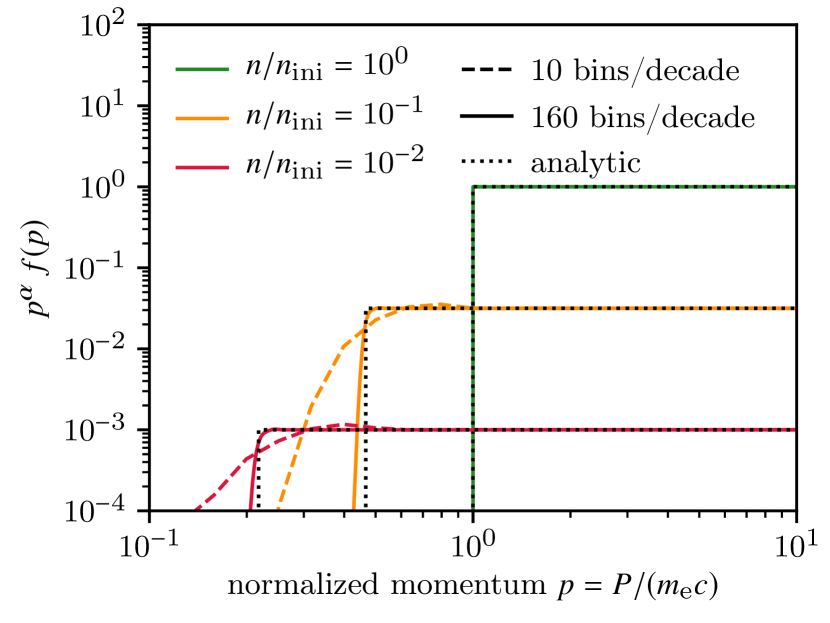
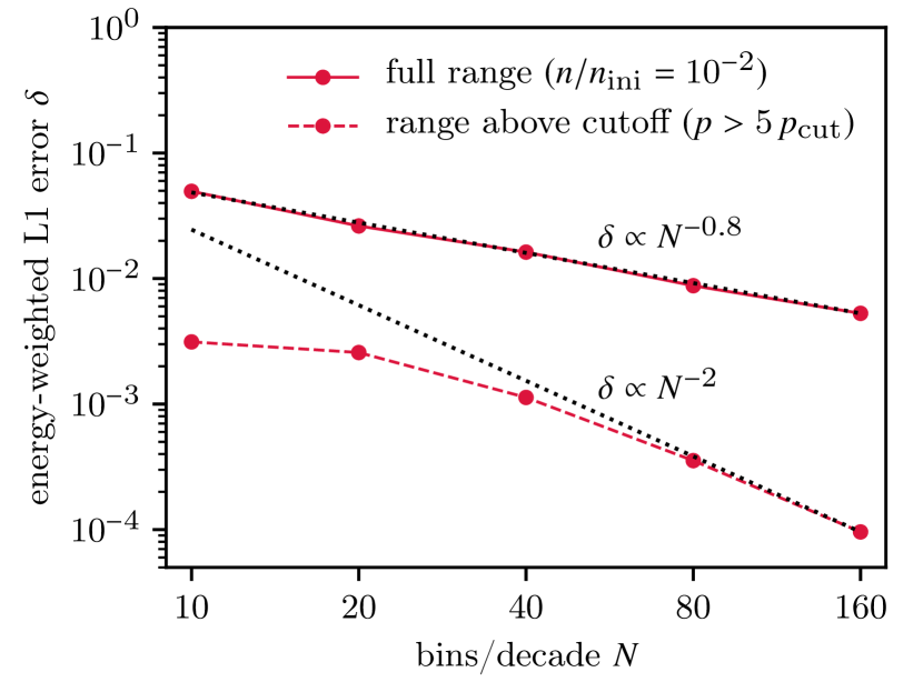
Figure 3: Adiabatic expansion of an initial power-law spectrum with $\alpha={2.5}$. Top: coloured dashed and solid lines represent the simulations with 10 and 160 bins per decade, respectively. The analytical solutions are shown as black dotted lines. Bottom: the energy-weighted relative L1 error for the entire momentum range and for momenta much larger than the cutoff of the analytical solution $p_{\mathrm{cut}}=10^{-2/3}$.

Adiabatic changes are mediated through the velocity divergence terms in equation (1). Due to phase space conservation upon adiabatic changes, a decreasing (increasing) gas density leads to decreasing (increasing) normalisation and a shift of the CR electron spectrum towards smaller (larger) momenta. In Figure 3, we follow the evolution of the spectrum during an adiabatic expansion over an expansion factor of $10^{-2}$. The energy-weighted L1 error between the simulated spectrum $f_{\mathrm{sim}}$ and the analytical spectrum $f_{\mathrm{ana}}$ is calculated according to the formula

$$\delta=\frac{\int\left|f_{\mathrm{sim}}(p)-f_{\mathrm{ana}}(p)\right|T(p)\differential{p}}{\int f_{\mathrm{ana}}(p)T(p)\differential{p}},$$ (60)

and decreases for increasing number of momentum bins $N$. The error scaling for the entire momentum range shows the effect of the slope limiter, which uses a second order accurate scheme for smooth parts of the spectrum and resorts to a first order scheme near jumps or strong gradients to prevent numerical oscillations. However, in the range above the cutoff the error scales as $\delta\propto N^{-2}$ as expected for a second-order accurate numerical scheme. We note that cooling and momentum diffusion normally lead to a smooth spectrum without sharp features. Hence, adiabatic changes are calculated with second-order accuracy.

3.2 Freely cooling spectrum

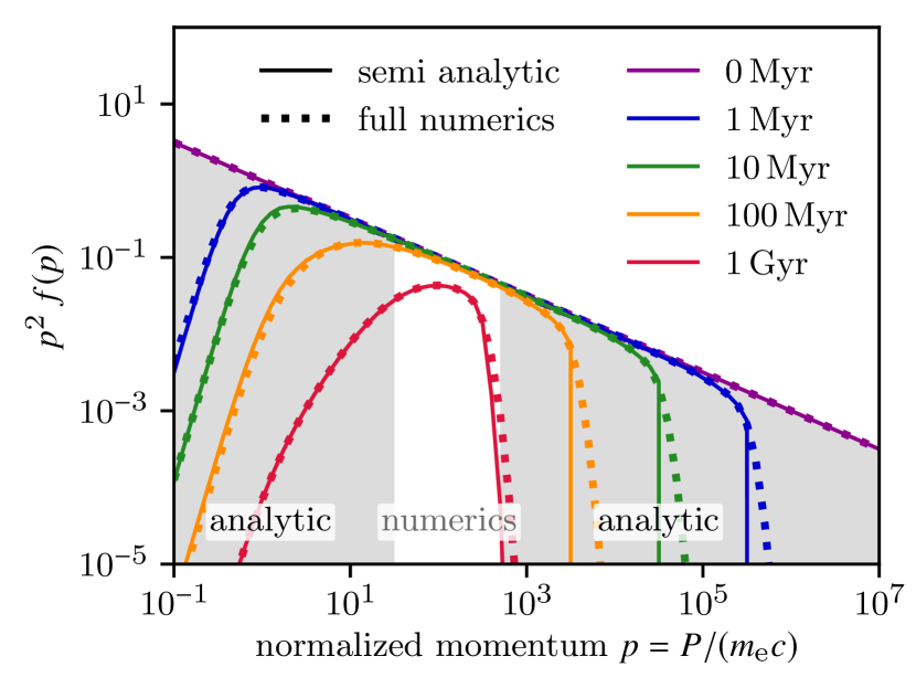
Figure 4: Freely cooling power-law spectrum with $\alpha=2.5$. We compare the fully numerical and semi-analytical solutions, for which we adopt analytical solutions in the shaded momentum range. The simulations use 10 bins per decade and the relevant parameters are ${n_{\mathrm{gas}}=10^{-3}\,\mathrm{cm}^{-3}}$, $B=$5\text{\,}\mathrm{\SIUnitSymbolMicro G}$$ and $\varepsilon_{\mathrm{ph}}=6\,\varepsilon_{\mathrm{cmb}}$.

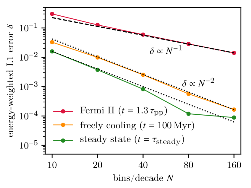
Figure 5: Energy-weighted relative L1 errors for cooling, steady-state and Fermi-II reacceleration tests.

A CR electron spectrum may experience cooling due to Coulomb, bremsstrahlung, inverse Compton and synchrotron losses. Figure 4 shows the cooling of an initial power-law spectrum with spectral index of $\alpha=2.5$ for a setup with 10 bins per decade. We compare the fully numerical solution to the semi-analytical solution, which uses the analytical solution in the shaded momentum ranges and the fully numerical solution in the range in between, where all cooling processes modify the initial power law. The fully numerical solution matches the semi-analytical solution except for the high-momentum cutoff which displays a larger diffusivity for the fully numerical scheme. The error of the fully numerical solution with $N$ bins is calculated according to equation (60) where we take the simulation with double resolution as $f_{\mathrm{ana}}\approx f_{2N}$. The error scaling is shown in Figure 5 and is second-order accurate, i.e. $\delta\propto N^{-2}$.

3.3 Steady-state spectrum

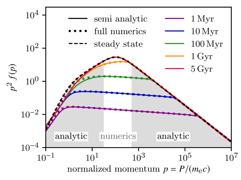
Figure 6: Build up of a steady-state spectrum due to continuous injection and cooling. The solid line and the dotted lines show the semi-analytical and the fully numerical simulations, respectively. The analytical steady-state solution is shown with a dashed line. The simulations use 10 bins per decade and a power-law source function with $\alpha=2.1$. The relevant parameters are $n_{\mathrm{gas}}=${10}^{-3}\text{\,}{\mathrm{cm}}^{-3}$$, $B=$5\text{\,}\mathrm{\SIUnitSymbolMicro G}$$ and $\varepsilon_{\mathrm{ph}}=6\,\varepsilon_{\mathrm{cmb}}$.

The combination of cooling and continuous source function $Q(p,t)$, e.g. acceleration or injection, in equation (1) leads to the build up of a self-similar spectrum. The self-similar spectrum agrees with the steady-state spectrum for momenta that have smaller cooling time-scales in comparison to the simulation time. Hence, the self-similar spectrum completely approaches the steady-state spectrum for very long times. We show this evolution in Figure 6 where we compare the results of the fully numerical and the semi-analytical simulations as well. Both simulations agree relatively well and approach the steady-state solution. However, there is a small deviation of the semi-analytical simulation visible in the Coulomb regime at around $p=1$. This is a consequence of the approximations adopted that enable an analytical solution for Coulomb cooling. Nevertheless, we prefer the semi-analytical simulation as it generally outperforms in efficiency in comparison to the fully numerical simulation (it is faster by a factor of $\sim 10^{4}$ for this specific setup). The error of the fully numerical solution compared to the analytical steady-state solution (see equations (37) and (60)) is shown in Figure 5 and scales with $\delta\propto N^{-2}$.

3.4 Fermi-II reacceleration

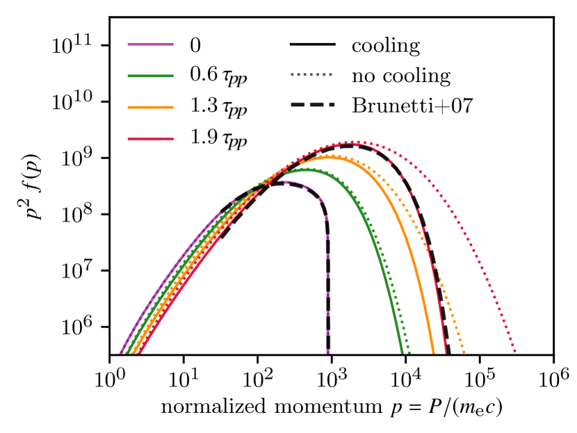
Figure 7: Fermi-II reacceleration with and without cooling of a relic spectrum in comparison to a reference study (Brunetti & Lazarian, 2007). The semi-analytical and fully numerical simulations that include cooling are indistinguishable. The relevant parameters are $n_{\mathrm{gas}}=${10}^{-3}\text{\,}{\mathrm{cm}}^{-3}$$, $B=$1\text{\,}\mathrm{\SIUnitSymbolMicro G}$$, $\varepsilon_{\mathrm{ph}}=\varepsilon_{\mathrm{cmb}}$ and $\tau_{\!p\!p}=$0.2\text{\,}\mathrm{G}\mathrm{y}\mathrm{r}$$. The time steps given in multiples of $\tau_{\!p\!p}$ are $0127254381\text{\,}\mathrm{M}\mathrm{y}\mathrm{r}$.

In addition to adiabatic changes, cooling, Fermi-I (re)acceleration, and injection, the CR electron spectrum may experience Fermi-II reacceleration, which is described by the momentum diffusion terms in equation (1) and which increases the energy of the spectrum. We adopt a typical value for the diffusion time of $\tau_{\!p\!p}=$0.2\text{\,}\mathrm{G}\mathrm{y}\mathrm{r}$$ in our tests. In Figure 7, we show two simulations with and without cooling for a high resolution of 160 bins per decade for Fermi-II reacceleration. Both simulations start with the same initial spectrum, which we have taken from a study on Fermi-II reacceleration of CR electrons by Brunetti & Lazarian (2007). The simulation with cooling approaches a limit for high momenta where cooling dominates over the reacceleration by the Fermi-II process. The result of the simulation with cooling matches the reference simulation by Brunetti & Lazarian (2007) very well. The simulation without cooling shows the main effect of Fermi-II reacceleration, i.e. diffusion in momentum space and a shift towards higher particle energies.

Figure 5 shows the error scaling of the different simulations with number of bins per momentum decade. The error is calculated with equation (60). However, for the simulations of freely cooling and momentum diffusion, we compare the result at given resolution $f_{N}$ to the double resolution, i.e. $f_{\mathrm{ana}}\approx f_{2N}$. The implemented Crank–Nicolson scheme is only accurate to first order in momentum space as can be seen by the $\delta\propto N^{-1}$ scaling. We consider this result for the Fermi-II reacceleration as a proof of concept. The improvement of the diffusion operator is straightforward but beyond the scope of this paper. The simulation of freely cooling and steady state show an error scaling of $\delta\propto N^{-2}$ which reflects our second-order accurate scheme for advection with a slope limiter.

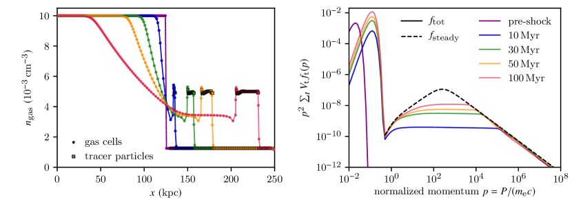
Figure 8: 1D shock-tube test of a strong shock ($\mathcal{M}=8.43,\alpha_{\mathrm{acc}}=2.0$) with 200 cells and 100 tracer particles. The left-hand panel shows the gas density profiles together with the tracer particles on which we evolve the CR electron spectra at different times. The right-hand panel shows the different total volume integrated thermal and CR electron spectra and the theoretically expected steady-state spectrum (dashed), for which we adopt $\alpha_{\mathrm{acc}}=2.02$ instead of the theoretical value $2.0$ to account for the numerical scatter of the shock compression ratio (see Figure 9). We adopt the parameters $B=$1\text{\,}\mathrm{\SIUnitSymbolMicro G}$$ and $\varepsilon_{\mathrm{ph}}=6\,\varepsilon_{\mathrm{cmb}}$.

4 Hydrodynamical simulations

In addition to idealised one-zone tests, we demonstrate that crest works in tandem with a hydrodynamical code. To this end, we use the second-order accurate, adaptive moving-mesh code arepo (Springel, 2010; Pakmor et al., 2016a) for simulations with ideal MHD (Pakmor & Springel, 2013). CR protons are modelled as a relativistic fluid with a constant adiabatic index of $\gamma_{\mathrm{crp}}=\ 4/3$ in a two-fluid approximation (Pfrommer et al., 2017a). We include Lagrangian tracer particles, which are velocity field tracers (Genel et al., 2013) and are passively advected with the gas and on which we solve the CR electron transport equation in post processing on every MHD time step.

To assess the validity of our setup, we investigate two different hydrodynamical scenarios, shock-tube simulations and 3D Sedov–Taylor blast-wave simulations. This enables us to probe Fermi-I acceleration and reacceleration, cooling and adiabatic processes in more realistic setups. The CR electron spectrum is calculated in post-processing separately for every tracer particle and the relevant parameters for the spectral evolution are taken from the gas cells which contain the tracer particles.

4.1 Shock tubes

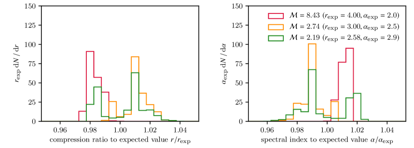
Figure 9: Histograms of the compression ratio (left-hand panel) and spectral index (right-hand panel), which are both normalised to their expected values for three different 1D shock-tube tests, which use the parameters given in table 1. The histograms account for all tracer particles at all time steps provided they experience an acceleration event.

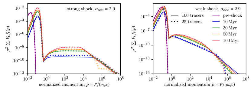
Figure 10: Tracer particle resolution study for 1D shock tubes of a strong shock (left-hand panel) and a weak shock (right-hand panel). The solid lines display the simulation with 100 tracer particles, which is for the strong shock identical to the right-hand panel in Figure 8, and the dotted line displays the simulation with 25 tracer particles. Low-resolution runs show temporary dips, but generally match the high-resolution runs well.

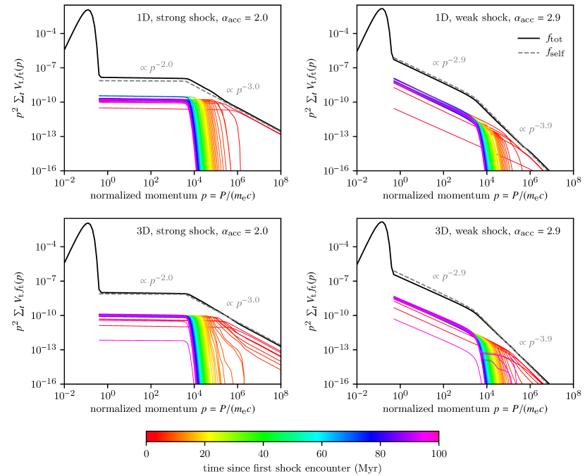
Figure 11: Total thermal and CR electron spectra at $100\text{\,}\mathrm{M}\mathrm{y}\mathrm{r}$ (black solid lines) and partial spectra of 100 time intervals since first shock encounter (coloured thin solid lines) for 1D and 3D shock-tube simulations (top and bottom, respectively) of strong and weak shocks (left- and right-hand panels, respectively). The theoretically expected steady-state spectrum (dashed) matches the total spectrum very well. Inverse Compton and synchrotron cooling lead to steeper spectra for large momenta. Note that Coulomb and bremsstrahlung cooling is neglected here.

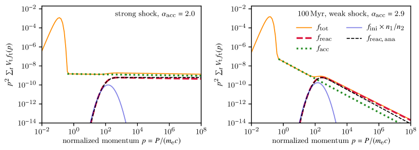
Figure 12: Comparison of direct acceleration (green dotted) and reacceleration (red dashed) without cooling in 1D shock-tube simulations for a strong and a weak shock (left- and right-hand panels, respectively). We show the initial relic spectrum (blue) and the total spectrum after the acceleration event (orange). The theoretically expected reacceleration spectrum matches the simulation very well.

Table 1: Initial values of our shock-tube setups. The parameters $n_{\mathrm{L}}=$1\text{\times}{10}^{-2}\text{\,}{\mathrm{cm}}^{-3}$$, $P_{\mathrm{th,L}}=$2.62\text{\times}{10}^{-11}\text{\,}\mathrm{erg}\text{\,}{\mathrm{cm}}^{-3}$$ and $P_{\mathrm{crp,L}}/P_{\mathrm{th,L}}=2$ for the left initial state and $n_{\mathrm{R}}=$0.125\text{\times}{10}^{-2}\text{\,}{\mathrm{cm}}^{-3}$$ and $P_{\mathrm{crp,R}}/P_{\mathrm{th,R}}=1$ for the right initial state are the same for all simulations.

$P_{\mathrm{th,R}}\ ($\mathrm{erg}\text{\,}{\mathrm{cm}}^{-3}$)$	$P_{\mathrm{th,L}}/P_{\mathrm{th,R}}$	$\mathcal{M}$	$r$	$\alpha_{\mathrm{acc}}$
$1.06\text{\times}{10}^{-13}$	247.0	$8.43$	$4.0$	$2.0$
$3.14\text{\times}{10}^{-13}$	23.4	$2.74$	$3.0$	$2.5$
$1.89\text{\times}{10}^{-12}$	13.9	$2.19$	$2.58$	$2.9$

First, we perform a series of shock-tube tests (Sod, 1978) in arepo with various shock strengths. The fluid is composed of gas and CR protons and we take CR acceleration at the shock in account (Pfrommer et al., 2017a) with CR proton shock acceleration efficiency of $\zeta_{\mathrm{crp}}=0.1$. In our 1D setups, we use a box with $250\text{\,}\mathrm{kpc}$ side length and 200 cells. In addition 100 tracer particles are located in the initial state on the right-hand side. For the 3D simulations, we use a box of dimension $250\times 25\times 25\,$\mathrm{kpc}$$ with $200\times 20\times 20$ cells and $100\times 10\times 10$ tracer particles in the initial state on the right-hand side. The tracer particles initially only contain a thermal electron spectrum. The initial states of the Sod shock-tube problem are laid down in table 1. We vary the thermal pressure $P_{\mathrm{th,R}}$ in order to obtain a desired Mach number $\mathcal{M}$ and 1D acceleration spectral index $\alpha_{\mathrm{acc}}$, which is a function of the shock compression ratio $r$, i.e. $\alpha_{\mathrm{acc}}=(r+2)/(r-1)$.

Figure 8 shows a 1D shock-tube test of a strong shock ($\mathcal{M}=8.43,\alpha_{\mathrm{acc}}=2.0$). The left-hand panel shows the gas density together with the tracer particles for different snapshots. The right-hand panel shows the thermal and CR electron spectra as a volume integrated sum of the tracer particle spectra, which have thermal spectra in the initial state. Except for the initial state at $t=0$, we sum up only spectra from those particles that have already encountered the shock front. Due to the initial inhomogeneity, a shock develops and propagates into the state on the right-hand side where the first tracer particle crosses the shock after $\sim 5\,\mathrm{Myr}$. As soon as a tracer particle encounters the shock front, CR electron acceleration is triggered, i.e. we use a source term of the form $Q_{\mathrm{e}}(p)\propto p^{-\alpha_{\mathrm{acc}}}$ in the transport equation (see equations (1) and (9)). The CR electron spectra experience losses due to Coulomb, bremsstrahlung, inverse Compton, and synchrotron interactions at the same time. Hence, the total spectrum has the form of a self-similar spectrum (see equation (36)).

The spectrum in Figure 8 approaches a steady state in the momentum regime, which has a shorter cooling time in comparison to the time since the first shock encounter. The total spectrum is similar to our idealised one-zone test, which simulates only one spectrum that experiences continuous cooling and injection. However, the simulation with arepo uses many tracer particles which experience acceleration only for limited amount of time when the particle resides in a shock surface or post shock cell of the hydrodynamical simulation. This clearly demonstrates that the combination of numerical and analytical solutions produces an effective, stable and accurate algorithm.

As pointed out before, the spectral index $\alpha_{\mathrm{acc}}$ of the accelerated spectrum depends on the shock compression ratio which is subject to numerical inaccuracies. In Figure 9, we show histograms for ratios of the numerically obtained value of shock compression to its expected value $r/r_{\mathrm{exp}}$ and ratios of the numerically obtained value of spectral index to its expected value $\alpha/\alpha_{\mathrm{exp}}$ for three different shock strengths (or equivalently Mach numbers). Here, we calculate the shock compression ratio with equation (29), which depends on the Mach number and which is formally only accurate for a single polytropic fluid. However, this calculation yields better results in comparison to the shock compression ratio directly calculated by the arepo shock finder. The resulting numerical error for the Mach number is typically better than one per cent (and deteriorates up to two per cent for weak shocks).

A resolution test of the number of tracer particles is shown in Figure 10, which displays the total spectra for 25 and 100 tracer particles for strong and weak shocks. The low-resolution spectra can show temporary dips due to poor sampling of the tracer particles in space, in particular at high momenta. However, low-resolution runs are stable and reproduce the general result of high-resolution runs. This demonstrates that our code produces stable and accurate results (only limited by the sampling rate) with respect to a coarser sampling of the tracer particles than the gas cells.

The total spectrum is a sum of all tracer particle spectra as we show in Figure 11. There, we plot the results of 1D and 3D simulations for strong and weak shocks. Note that we only consider inverse Compton and synchrotron cooling for clarity. Each panel shows the total spectrum, the theoretically expected self-similar spectrum, and partial sums of spectra of 100 equally spaced time intervals since the first shock encounter. Those particles that have most recently crossed the shock (red lines) experience simultaneously acceleration and cooling and show a self-similar spectrum. The spectra of those particles that have encountered the shock some time ago (orange to purple lines) show an exponential high-momentum cutoff resulting from the freely cooling CR electron population. The total spectrum has the slope of the acceleration spectrum for those momenta which have cooling times longer than $100\text{\,}\mathrm{M}\mathrm{y}\mathrm{r}$, i.e. $p\lesssim 10^{4}$ for these setups. At larger momenta, $p\gtrsim 10^{4}$ , the slope of the total spectrum steepens to $\alpha_{\mathrm{acc}}+1$ as expected from equation (46). The total spectra for all setups match the theoretically expected self-similar spectra very well, although slight deviations are visible. These follow from the numerical scatter of the shock compression ratio in arepo. We note that the computation of the CR electron spectrum with crest is faster than the hydrodynamical simulation by a factor of about 20 in the 3D shock-tube simulations.

In addition to direct acceleration of primary CR electrons at the shock, a previously existing non-thermal CR electron population can be reaccelerated at the shock. We show the resulting spectra for a strong and a weak shock after $100\text{\,}\mathrm{M}\mathrm{y}\mathrm{r}$ in Figure 12. The setups are similar to the simulations presented above except for the previously existing non-thermal relic spectrum and except for the fact that we deactivated CR electron cooling for clarity here. As soon as a tracer particle encounters the shock, it experiences both, reacceleration of the initial relic spectrum and direct acceleration of a primary power-law spectrum. Each panel shows the initial relic spectrum (blue), the total spectrum after the acceleration event (orange), the directly accelerated spectrum (green dashed line), and the reaccelerated spectrum (red dashed line). The theoretically expected reaccelerated spectrum is also shown (black dashed line) and matches the simulated reacceleration spectrum. The slope of the reaccelerated spectrum in the weak-shock case deviates slightly from its theoretical expectation because of numerical scatter of the shock compression ratio (see Figure 9).

In the case of a strong shock, the primary accelerated spectrum dominates over the reaccelerated spectrum, hence the total spectrum is only weakly modified by reacceleration (see Figure 12). In contrast, the reaccelerated spectrum dominates the total spectrum for large momenta at weak shocks. This is important for observable signatures such as, e.g. the flux of radio emission. We note that the relative strength between direct acceleration and reacceleration depends on the details of shock acceleration, which we do not resolve with our hydrodynamical simulations. In our setup, we convert a fixed fraction of the accelerated CR proton energy into CR electrons at the shock which leads to a larger normalisation for steeper spectra. Other shock acceleration models, e.g. thermal leakage models (Kang & Ryu, 2011), predict different relative strengths of reacceleration to direct acceleration.

4.2 Sedov–Taylor blast wave

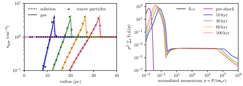
Figure 13: 3D Sedov–Taylor blast-wave simulation with $200^{3}$ gas cells and $\sim 30^{3}$ tracer particles. The left-hand panel shows the radial gas density profile (solid), the theoretical solution (dashed) and the spherically-averaged density of the tracer particles within concentric shells (points) for different times. The right-hand panel shows the total initial thermal spectrum (purple) and the total spectrum of particles, which have crossed the shock, at four characteristic times.

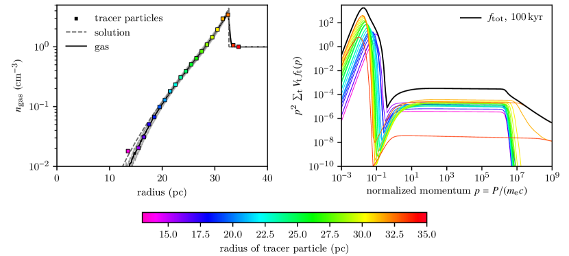
Figure 14: Spherically-averaged tracer particle density (left-hand panel) and the contribution of tracer particles to the total spectrum (right-hand panel) for the 3D Sedov–Taylor blast-wave simulation at $100\text{\,}\mathrm{k}\mathrm{y}\mathrm{r}$. The colour indicates the different radii of tracer particles, which correspond to different times since shock crossing. The radial bins for the tracer particles have a width of $1\text{\,}\mathrm{p}\mathrm{c}$ and the grey band denotes the density scatter of the simulation.

In addition to the shock-tube tests we perform simulations of spherical shocks in order to test acceleration and cooling in tandem with adiabatic CR electron expansion. We setup a 3D Sedov–Taylor problem with an energy-driven spherical shock which expands into a medium with negligible pressure. We use a symmetric 3D box with $200^{3}$ cells, $100\text{\,}\mathrm{pc}$ side length and the following parameters for the initial conditions: The gas number density of the ambient medium is $n_{\mathrm{gas}}=$1\text{\,}{\mathrm{cm}}^{-3}$$, has a temperature of $T=${10}^{4}\text{\,}\mathrm{K}$$ and a thermal adiabatic index of $\gamma_{\mathrm{th}}=5/3$. We inject an initial thermal energy of $E_{0}=${10}^{51}\text{\,}\mathrm{e}\mathrm{r}\mathrm{g}$$ into the central cell. The tracer particles are initially located on a regular Cartesian mesh with $30^{3}$ grid points of which we excise a small spherical region around the centre. The tracer particles initially only contain a thermal electron spectrum.

The left-hand panel of Figure 13 shows the simulated gas density profile for different snapshots together with the theoretical solution and the spherically-averaged density of the tracer particles within concentric shells. As expected for a single polytropic fluid, the shock radius of the 3D explosion evolves as

$$r_{\mathrm{shock}}(t)=\left(\frac{E_{0}}{\alpha\rho_{0}}\right)^{1/5}t^{2/5},$$ (61)

where $\rho_{0}$ is the ambient mass density and $\alpha$ the self-similarity parameter of the Sedov (1959) solution. In our simulation, we adopt a CR shock acceleration efficiency of $\zeta_{\mathrm{CR}}=0.1$, which yields an effective adiabatic index $\gamma_{\mathrm{eff}}=1.58$ and a self-similarity parameter $\alpha=0.57$ (Pais et al., 2018). We note that the tracer particles experience a slightly smaller density jump of $r\approx 4$ in comparison to the theoretically expected value of $r=4.45$ in this setup due to the narrow density jump of the theoretical solution and the limited spatial resolution of the hydrodynamical simulation.

The right-hand panel of Figure 13 shows the total electron spectrum, where we only take the spectrum of those particles into account which have already crossed the shock front except for the initial spectrum with all tracer particles. It is apparent that the total spectrum is approximately constant for all snapshots at momenta $10^{1}\lesssim p\lesssim 10^{6}$ where the time-scales of Coulomb, inverse Compton, and synchrotron cooling are longer than our simulation time. This is a consequence of constant kinetic and total energy of the shock of a Sedov–Taylor blast wave. In the thin-shell approximation, all mass is contained in a shell of radius $r_{\mathrm{shock}}$ that expands with velocity $\varv_{\mathrm{post}}=2\varv_{\mathrm{shock}}/(\gamma_{\mathrm{eff}}+1)$, which yields a constant kinetic energy of $E_{\mathrm{kin}}=32\pi E_{0}/\left[75\alpha(\gamma_{\mathrm{eff}}+1)^{2}\right]\approx 0.35E_{0}$. A fraction of this energy goes into CR electrons, and particles that have recently crossed the shock dominate the spectrum. We note that we obtain robust results for the CR electron spectrum although the tracer particles are more coarsely sampled than the gas cells by a factor of $\sim 6^{3}$.

The contribution to the total spectrum of tracer particles at different radii is shown in Figure 14. Red lines represent the radial bin at which only a fraction of tracer particles experience shock acceleration. Hence, their spectra are subdominant to the total spectrum. The total spectrum is dominated by particles whose distance to the centre is close the maximum of the radial gas density profile as they all experience shock acceleration and have not yet lost energy due to adiabatic expansion. Yellow to purple lines represent particles which are located towards inner radii and which are effected by cooling due to adiabatic expansion and non-adiabatic processes. These tests demonstrate that our code also handles adiabatic expansion together with acceleration and cooling of CR electrons. We note that the CR electron spectrum is efficiently calculated with crest, which is faster than the hydrodynamical simulation by a factor of about 460.

5 Conclusions

We have presented our stand-alone post-processing code crest that evolves the spectra of CR electrons on Lagrangian trajectories spatially and temporally resolved. So far, we model the spatial CR electron transport as advection with the gas and defer modelling CR electron streaming and (spatial) diffusion to future work. All important physical cooling processes of CR electrons are included, i.e. adiabatic expansion, Coulomb cooling, and radiative processes such as inverse Compton, synchrotron and bremsstrahlung cooling. In addition to adiabatic compression, we account for non-adiabatic energy gain processes such as diffusive shock acceleration and reacceleration as well as Fermi-II reacceleration via particle interactions with compressible turbulence.

The CR electron cooling times at very low and very high momenta are much smaller than typical time steps in simulations of galaxy formation or the ISM. Hence, we develop a hybrid algorithm that combines numerical and analytical solutions to the Fokker–Planck equations such that the resulting code works efficiently and accurately on the MHD time step. We demonstrate in a number of code validation simulations that the result of our hybrid algorithm is as good as the fully numerical solution, which is however computationally considerably more expensive. This hybrid treatment decreases the computational cost of evolving the CR electron spectrum and renders cosmological simulations with CR electrons feasible.

crest has been extensively tested in idealized one-zone models and alongside hydrodynamical simulations of the arepo code. Idealized one-zone tests demonstrate that isolated terms of the Fokker–Planck equation are accurately captured with our code. The arepo simulations show (i) that crest works very well and efficiently together with a hydrodynamical code at almost negligibly additional computational cost, (ii) that the total spectrum, which is the sum of singular spectra on tracer particles, evolves as expected, and (iii) that the spatial sampling of the tracer particles quickly converges with increasing number of tracer particles. In particular, our results are robust to a coarser sampling of the tracer particles in comparison to the resolution of our unstructured mesh. Future studies will show how the spectral properties depend on the spatial sampling rate in more complex simulations of realistic environments. We note that our algorithm (and code) can in principle be combined with every (magneto)hydrodynamical code that has Lagrangian tracer particles on which the comoving Fokker–Planck equations for the CR electron spectrum is solved.

The presented method allows studying the evolution of the CR electron spectrum in the ISM, in galaxies and galaxy clusters as well as for AGN jets in great detail. It enables to link the non-thermal physics to observables such as $\gamma$-ray and radio measurements and to distinguish leptonic and hadronic emission scenarios. These include SNRs where we can gain insight which environmental parameter (mean density, density fluctuations, magnetic field strength) determines the dominating emission scenario. It will further allow us to perform self-consistent studies on the evolution of the Fermi bubbles or galactic outflows in MHD simulations and to test models that rely on star formation or on AGN activity. This insight will be key for a more profound understanding of the most important feedback processes during the formation of galaxies. Finally, our code crest will enable us to self-consistently follow the CR electron spectrum during the evolution of galaxy clusters, it can possibly help to understand the enigmatic formation scenarios of radio relics and radio haloes and how they relate to the dynamical state of clusters.

Appendix A Numerical solution to the Fokker–Planck equation

Here, we present details of the advection and diffusion operator. In the following, $f_{i}^{n}=f(p_{i},t_{n})$ denotes the value of the spectrum at momentum $p_{i}$ and time $t_{n}$.

A.1 Advection operator

Our advection operator accounts for cooling (i.e. Coulomb, bremsstrahlung, inverse Compton, and synchrotron cooling), adiabatic changes, and particle acceleration. In our code, we treat Fermi-I acceleration and reacceleration as continuous injection via the term $Q(p,t)$ in equation (1) as long as the tracer particle resides in shock surface and post-shock cells, i.e. we treat CR electron acceleration identically to the model for CR proton acceleration described by Pfrommer et al. (2017a). The advection problem obeys the reduced equation

$$\left.\derivative{f(p,t)}{t}\right|_{\mathrm{adv}} -\partialderivative{p}\left\{f(p,t)\left[\frac{p}{3}\left(\divergence{{\bf\it\varv}}\right)-\dot{p}(p,t)\right]\right\}=$$

$$-\left(\divergence{{\bf\it\varv}}\right)f(p,t)+Q(p,t),$$ (62)

where $\derivative*{t}=\partial/\partial t+\boldsymbol{\varv\cdot\nabla}$ is the Lagrangian time derivative.

We discretise this equation with a flux-conserving finite volume scheme using a second-order piecewise linear reconstruction of the spectrum (LeVeque et al., 1998). In addition, we use the non-linear van Leer flux limiter (van Leer, 1977) and treat the terms on the right-hand side as an inhomogeneity.

All following equations have in principle to be carried out for all $N$ momentum bins, i.e. $i\in\left[0,\,N{-}1\right]$. The spectrum significantly decreases due to rapidly cooling at low and high momenta. We thus cut the spectrum at $f_{\mathrm{cut}}$ below which we treat numerical values of the spectrum as zero. The related indices $i_{\mathrm{lcut}}$ and $i_{\mathrm{hcut}}$ are defined in equations (22) and (23), respectively. The indices $i_{\mathrm{low}}$ and $i_{\mathrm{high}}$ of the transition momenta between the analytical and numerical solutions are defined in equations (55) and (56). This further limits the momentum range of the advection solver. We define two limiting indices of the advection operator

$$i_{\mathrm{ladv}}=\max\mathopen{}\left(i_{\mathrm{lcut}},i_{\mathrm{low}}\right)\mbox{ and}$$ (63)

$$i_{\mathrm{hadv}}=\min\mathopen{}\left(i_{\mathrm{hcut}},i_{\mathrm{high}}\right)$$ (64)

for which $0\leq i_{\mathrm{ladv}}$ and $i_{\mathrm{hadv}}\leq N$ hold. In the case of a fully numerical simulation, the limiting indices of the advection operator are $i_{\mathrm{ladv}}=i_{\mathrm{lcut}}$ and $i_{\mathrm{hadv}}=i_{\mathrm{hcut}}$.

Because the total cooling time-scale $[\dot{p}(p)/p]^{-1}$ is a convex function of momentum, the shortest cooling time-scale is determined by the smallest or largest momentum of the momentum range which is treated by the advection operator. As the numerical scheme calculates fluxes between bins, we evaluate the maximum function over the cooling rates in equation (18) on the outermost bin edges and use

$$\max\mathopen{}\left(\frac{\absolutevalue{\dot{p}(p)}}{\Delta p}\right)=\max\mathopen{}\left(\frac{\dot{p}\mathopen{}\left(p_{i_{\mathrm{ladv}}+3/2}\right)}{p_{i_{\mathrm{ladv}}+2}-p_{i_{\mathrm{ladv}}+1}},\frac{\dot{p}\mathopen{}\left(p_{i_{\mathrm{hadv}}-5/2}\right)}{p_{i_{\mathrm{hadv}}-1}-p_{i_{\mathrm{hadv}}-2}}\right).$$ (65)

The advection operator has a symmetric stencil of five bins which makes in total four ghost bins, with indices $i_{\mathrm{ladv}}$, $i_{\mathrm{ladv}}{+}1$, $i_{\mathrm{hadv}}{-}2$, and $i_{\mathrm{hadv}}{-}1$, necessary. The function values on these bins are determined by power-law extrapolation.

The advection operator works as follows. First, we explicitly evolve the spectrum under the influence of (re)acceleration and injection by a half time step

$$f_{i}^{n+1/2}=f_{i}^{n}+\frac{\Delta t}{2}Q_{i}^{n}$$ (66)

where $Q_{i}^{n}=Q(p_{i},t_{n})$ denotes the discretised (re)acceleration and injection rate at momentum $p_{i}$ and time $t_{n}$ (see equations (27) and (28)). We define the advection velocity of momentum bin $p_{i}$ at time $t_{n}$ due to adiabatic and cooling processes by

$$u_{i}^{n}=\frac{p_{i}}{3}\left(\divergence{{\bf\it\varv}}\right)-\dot{p}(p_{i})\mbox{ at time }t_{n}.$$ (67)

The advection velocity of the bin edges $u_{i-1/2}$ is similarly defined. We use the advection velocities and the partly evolved function values $f_{i}^{n+1/2}$ from equation (66) to calculate fluxes $F$ through the bin edges at intermediate time $t_{n+1/2}$. Depending on the sign of the advection velocity $u_{i-1/2}$ at the bin edge, the flux is given by

$$F_{i-1/2}^{n+1/2}=\begin{aligned} &u_{i-1}f_{i-1}^{n+1/2}\\ &+\phi(r_{i-1})\sigma_{i-1/2}\left(p_{i-1/2}-p_{i-1}+u_{i-1/2}\frac{\Delta t}{2}\right)\end{aligned}$$ (68)

for negative advection velocities $u_{i-1/2}<0$ and by

$$F_{i-1/2}^{n+1/2}=\begin{aligned} &u_{i}f_{i}^{n+1/2}\\ &-\phi(r_{i})\sigma_{i-1/2}\left(p_{i}-p_{i-1/2}-u_{i-1/2}\frac{\Delta t}{2}\right)\end{aligned}$$ (69)

for positive advection velocities $u_{i-1/2}\geq 0$. The variable $\sigma_{i}$ is the slope of the function values between two bins weighted with their advection velocities

$$\sigma_{i-1/2}=\frac{u_{i}f_{i}^{n+1/2}-u_{i-1}f_{i-1}^{n+1/2}}{p_{i}-p_{i-1}}.$$ (70)

The function $\phi(r)$ is the slope limiter function, for which we use the van-Leer slope limiter

$$\phi(r_{i})=\frac{r_{i}+\absolutevalue{r_{i}}}{1+\absolutevalue{r_{i}}}.$$ (71)

The variable $r_{i}$ is ratio of slope at the left bin edge to the slope at the right bin edge, whose definition depends on the sign of the advection velocity. For negative advection velocities $u_{i-{1/2}}<0$, we use

$$r_{i-1}=\frac{u_{i-1}f_{i-1}^{n+{1/2}}-u_{i-2}f_{i-2}^{n+{1/2}}}{p_{i-1}-p_{i-2}}\frac{p_{i}-p_{i-1}}{u_{i}f_{i}^{n+{1/2}}-u_{i-1}f_{i-1}^{n+{1/2}}}$$ (72)

and for positive advection velocities $u_{i-{1/2}}\geq 0$, we adopt

$$r_{i}=\frac{u_{i+1}f_{i+1}^{n+{1/2}}-u_{i}f_{i}^{n+{1/2}}}{p_{i-1}-p_{i-2}}\frac{p_{i}-p_{i-1}}{u_{i}f_{i}^{n+{1/2}}-u_{i-1}f_{i-1}^{n+{1/2}}}.$$ (73)

We use the fluxes $F^{n+1/2}$ at intermediate time step $t_{n+1/2}$ with the half time step estimate of the spectrum $f^{n+1/2}$ to calculate the spectrum at time $t_{n+1}$

$$f_{i}^{n+1}=\begin{aligned} &f_{i}^{n+{1/2}}\left(1-\Delta t\left(\divergence{{\bf\it\varv}}\right)\right)+\frac{\Delta t}{2}Q_{i}\\ &+\Delta t\frac{F_{i+{1/2}}-F_{i-{1/2}}}{p_{i+{1/2}}-p_{i-{1/2}}}\left(1-\frac{\Delta t}{2}\left(\divergence{{\bf\it\varv}}\right)\right),\end{aligned}$$ (74)

where we included an additional factor $\left(1-\Delta t/2\left(\divergence{{\bf\it\varv}}\right)\right)$ that results from the influence of adiabatic changes on the fluxes.

A.2 Diffusion operator

The diffusion operator is based on the Crank–Nicolson method and solves the diffusive part of the CR electron Fokker–Planck equation (1),

$$\left.\derivative{f(p,t)}{t}\right|_{\mathrm{diff}}+\partialderivative{p}\left[\frac{f(p,t)}{p^{2}}\partialderivative{p}(p^{2}D_{\!p\!p})\right]-\partialderivative[2]{p}\left[D_{\!p\!p}f(p,t)\right]=0.$$ (75)

The combination of an explicit solution

$$f_{i}^{n+1}=\alpha_{i}f_{i-1}^{n\phantom{+1}}+(1-\beta_{i})f_{i}^{n\phantom{+1}}+\gamma_{i}f_{i+1}^{n\phantom{+1}}$$ (76)

and an implicit solution

$$f_{i}^{n\phantom{+1}}=-\alpha_{i}f_{i-1}^{n+1}+(1+\beta_{i})f_{i}^{n+1}-\gamma_{i}f_{i+1}^{n+1}$$ (77)

yields the semi-implicit Crank–Nicolson scheme

$$\begin{aligned} &-\frac{\alpha_{i}}{2}f_{i-1}^{n+1}+\left(1+\frac{\beta_{i}}{2}\right)f_{i}^{n+1}-\frac{\gamma_{i}}{2}f_{i+1}^{n+1}\\ &\qquad=\frac{\alpha_{i}}{2}f_{i-1}^{n}+\left(1-\frac{\beta_{i}}{2}\right)f_{i}^{n}+\frac{\gamma_{i}}{2}f_{i+1}^{n}.\end{aligned}$$ (78)

The coefficients $\alpha_{i},\beta_{i}$, and $\gamma_{i}$ are derived by discretising the momentum diffusion term,

$$\begin{aligned} \alpha_{i}&=\left[\frac{D_{i}}{p_{i+1/2}-p_{i-1/2}}+\frac{2D_{i-1}}{p_{i-1}}\right]\frac{\Delta t}{p_{i}-p_{i-1}},\\ \beta_{i}&=\bigg{[}\begin{aligned} &\frac{D_{i}}{p_{i}(p_{i}-p_{i-1})}+\frac{D_{i+1}-D_{i}}{(p_{i+1}-p_{i})^{2}}\\ &+\frac{D_{i}}{p_{i+1/2}-p_{i-1/2}}\left(\frac{1}{p_{i+1}-p_{i}}+\frac{1}{p_{i}-p_{i-1}}\right)\bigg{]}\Delta t,\end{aligned}\\ \gamma_{i}&=\left[\frac{D_{i}}{(p_{i+1}-p_{i})(p_{i+1/2}-p_{i-1/2})}+\frac{D_{i+1}-D_{i}}{(p_{i+1}-p_{i})^{2}}\right]\Delta t,\end{aligned}$$ (79)

where we have used the abbreviation $D_{i}=D_{\!p\!p}(p_{i})$ and the time step $\Delta t$. The diffusion time step is defined in equation (19) which is

$$\Delta t=\frac{C_{\mathrm{CFL}}}{D_{0}}$$ (80)

with $D_{\!p\!p}=D_{0}p^{2}$ (see equation (13)). Equation (78) can be written as matrix equation

$$\textbf{{A}}\boldsymbol{\cdot}\textbf{{f}}^{n+1}=\textbf{{B}}\boldsymbol{\cdot}\textbf{{f}}^{n},$$ (81)

where $\textbf{{A}},~{}\textbf{{B}}$ are $(N\times N)$ matrices

$$\begin{aligned} &\textbf{{A}}=\begin{pmatrix}b_{0}&0&&&&\\ a_{1}&b_{1}&c_{1}&&&\\ &a_{2}&b_{2}&c_{2}&&\\ &&\ddots&\ddots&\ddots&\\ &&&a_{N-2}&b_{N-2}&c_{N-2}\\ 0&&&&0&b_{N-1}\end{pmatrix}\\ &\textbf{{B}}=\begin{pmatrix}1&0&&&&\\ \tilde{a}_{1}&\tilde{b}_{1}&\tilde{c}_{1}&&&\\ &\tilde{a}_{2}&\tilde{b}_{2}&\tilde{c}_{2}&&\\ &&\ddots&\ddots&\ddots&\\ &&&\tilde{a}_{N-2}&\tilde{b}_{N-2}&\tilde{c}_{N-2}\\ &&&&0&1\end{pmatrix}\end{aligned}$$ (82)

and $\textbf{{f}}^{n}$ and $\textbf{{f}}^{n+1}$ are $N$-dimensional vectors containing the values of the CR electron spectrum in every momentum bin at time $t_{n}$ and $t_{n+1}$ respectively, i.e. $\textbf{{f}}^{n}=(f_{i}^{n})$ and $\textbf{{f}}^{n+1}=(f_{i}^{n+1})$. The coefficients of the matrices A and B are

$$\ \begin{matrix}a_{i}=-\frac{\alpha_{i}}{2},&b_{i}=1+\frac{\beta_{i}}{2},&c_{i}=-\frac{\gamma_{i}}{2},\\ \tilde{a}_{i}=\frac{\alpha_{i}}{2},&\tilde{b}_{i}=1-\frac{\beta_{i}}{2},&\tilde{c}_{i}=\frac{\gamma_{i}}{2},\end{matrix}$$ (83)

for $i\in\left[1,\,N{-}2\right]$, whereas the coefficients $b_{0}=f_{0}^{n}/f_{0}^{n+1}$ and $b_{N-1}=f_{N-1}^{n}/f_{N-1}^{n+1}$ are chosen in order to fulfill the boundary conditions. In order to solve equation (81), the tridiagonal matrix A is inverted with the Thomas algorithm, also known as tridiagonal matrix algorithm. If we write $\textbf{{d}}=\textbf{{B}}\boldsymbol{\cdot}\textbf{{f}}^{n}$, the matrix equation (81) takes the from

$$\begin{pmatrix}b_{0}&0&&&&\\ a_{1}&b_{1}&c_{1}&&&\\ &a_{2}&b_{2}&c_{2}&&\\ &&\ddots&\ddots&\ddots&\\ &&&a_{N-2}&b_{N-2}&c_{N-2}\\ &&&&0&b_{N-1}\end{pmatrix}\begin{pmatrix}f_{0}^{n+1}\\ f_{1}^{n+1}\\ f_{2}^{n+1}\\ \vdots\\ f_{N-2}^{n+1}\\ f_{N-1}^{n+1}\end{pmatrix}=\begin{pmatrix}d_{0}\\ d_{1}\\ d_{2}\\ \vdots\\ d_{N-2}\\ d_{N-1}\end{pmatrix}$$ (84)

and its solution is numerically obtained by the application of the forward calculations

$$c_{i}^{\prime}=\left\{\begin{array}[]{ll}\frac{c_{i}}{b_{i}}&\mbox{for }i=0,\\ \frac{c_{i}}{b_{i}-a_{i}c_{i-1}^{\prime}}&\mbox{for }i=1,\,\ldots,\,N{-}1,\end{array}\right.$$ (87)

$$d_{i}^{\prime}=\left\{\begin{array}[]{ll}\frac{d_{i}}{b_{i}}&\mbox{for }i=0,\\ \frac{d_{i}-a_{i}d_{i-1}^{\prime}}{b_{i}-a_{i}c_{i-1}^{\prime}}&\mbox{for }i=1,\,\ldots,\,N{-}1,\end{array}\right.$$ (90)

and of the backward calculation

$$f_{i}^{n+1}=\left\{\begin{array}[]{ll}d_{i}^{\prime}&\mbox{for }i=N{-}1,\\ d_{i}^{\prime}-c_{i}^{\prime}f_{i+1}^{n+1}&\mbox{for }i=N{-}2,\,\ldots,\,0.\end{array}\right.$$ (93)

We note that the amount of calculations can be reduced if we take only bins into account where the spectrum is larger than a given low cut $f_{\mathrm{cut}}$. In this case, equation (81) reduces to an $M$-dimensional matrix equation with $M=i_{\mathrm{hcut}}-i_{\mathrm{lcut}}$ and the matrix inversion has to be applied for a submatrix, which is characterised by the indices $i_{\mathrm{lcut}},\,i_{\mathrm{lcut}}{+}1,\,i_{\mathrm{lcut}}{+}2,\,\ldots,\,i_{\mathrm{hcut}}{-}2,\,i_{\mathrm{hcut}}{-}1$.

References

- Battaglia et al. (2009) Battaglia N., Pfrommer C., Sievers J. L., Bond J. R., Enßlin T. A., 2009, MNRAS, 393, 1073
- Bell (1978) Bell A. R., 1978, MNRAS, 182, 443
- Bell (2004) Bell A. R., 2004, MNRAS, 353, 550
- Benaglia et al. (2010) Benaglia P., Romero G. E., Martí J., Peri C. S., Araudo A. T., 2010, A&A, 517, L10
- Blandford & Eichler (1987) Blandford R., Eichler D., 1987, Phys. Rep., 154, 1
- Blasi (2013) Blasi P., 2013, A&ARv, 21, 70
- Booth et al. (2013) Booth C. M., Agertz O., Kravtsov A. V., Gnedin N. Y., 2013, ApJ, 777, L16
- Boulares & Cox (1990) Boulares A., Cox D. P., 1990, ApJ, 365, 544
- Breitschwerdt et al. (1991) Breitschwerdt D., McKenzie J. F., Voelk H. J., 1991, A&A, 245, 79
- Brezinski (1996) Brezinski C., 1996, Appl. Numer. Math., 20, 299
- Brunetti & Lazarian (2007) Brunetti G., Lazarian A., 2007, MNRAS, 378, 245
- Brunetti & Lazarian (2011) Brunetti G., Lazarian A., 2011, MNRAS, 412, 817
- Bykov et al. (2018) Bykov A. M., Ellison D. C., Marcowith A., Osipov S. M., 2018, Space Science Reviews, 214, 41
- Bykov et al. (2019) Bykov A. M., Vazza F., Kropotina J. A., Levenfish K. P., Paerels F. B. S., 2019, Space Sci. Rev., 215, 14
- Carretti et al. (2013) Carretti E., et al., 2013, Nature, 493, 66
- Celli et al. (2019) Celli S., Morlino G., Gabici S., Aharonian F. A., 2019, MNRAS, 487, 3199
- Dobler et al. (2010) Dobler G., Finkbeiner D. P., Cholis I., Slatyer T., Weiner N., 2010, ApJ, 717, 825
- Donnert & Brunetti (2014) Donnert J., Brunetti G., 2014, MNRAS, 443, 3564
- Donnert et al. (2013) Donnert J., Dolag K., Brunetti G., Cassano R., 2013, MNRAS, 429, 3564
- Drury (1983) Drury L. O., 1983, Reports on Progress in Physics, 46, 973
- Dubois & Commerçon (2016) Dubois Y., Commerçon B., 2016, A&A, 585, A138
- Ehlert et al. (2018) Ehlert K., Weinberger R., Pfrommer C., Pakmor R., Springel V., 2018, MNRAS, 481, 2878
- Ellison et al. (2012) Ellison D. C., Slane P., Patnaude D. J., Bykov A. M., 2012, ApJ, 744, 39
- Enßlin et al. (1998) Enßlin T. A., Biermann P. L., Klein U., Kohle S., 1998, A&A, 332, 395
- Enßlin et al. (2007) Enßlin T. A., Pfrommer C., Springel V., Jubelgas M., 2007, A&A, 473, 41
- Enßlin et al. (2011) Enßlin T., Pfrommer C., Miniati F., Subramanian K., 2011, A&A, 527, A99
- Everett et al. (2008) Everett J. E., Zweibel E. G., Benjamin R. A., McCammon D., Rocks L., Gallagher III J. S., 2008, ApJ, 674, 258
- Fermi (1949) Fermi E., 1949, Physical Review, 75, 1169
- Fujita & Ohira (2012) Fujita Y., Ohira Y., 2012, ApJ, 746, 53
- Genel et al. (2013) Genel S., Vogelsberger M., Nelson D., Sijacki D., Springel V., Hernquist L., 2013, MNRAS, 435, 1426
- Girichidis et al. (2016) Girichidis P., et al., 2016, ApJ, 816, L19
- Girichidis et al. (2018) Girichidis P., Naab T., Hanasz M., Walch S., 2018, MNRAS, 479, 3042
- Gould (1972) Gould R. J., 1972, Physica, 60, 145
- Guo & Oh (2008) Guo F., Oh S. P., 2008, MNRAS, 384, 251
- Guo et al. (2014a) Guo X., Sironi L., Narayan R., 2014a, ApJ, 794, 153
- Guo et al. (2014b) Guo X., Sironi L., Narayan R., 2014b, ApJ, 797, 47
- Hanasz & Lesch (2003) Hanasz M., Lesch H., 2003, A&A, 412, 331
- Hanasz et al. (2010) Hanasz M., Kowalik K., Wóltański D., Pawłaszek R., 2010, in Gożdziewski K., Niedzielski A., Schneider J., eds, EAS Publications Series Vol. 42, EAS Publications Series. pp 275–280 (arXiv:0812.2161), doi:10.1051/eas/1042029, http://adsabs.harvard.edu/abs/2010EAS....42..275H
- Heesen et al. (2016) Heesen V., Dettmar R.-J., Krause M., Beck R., Stein Y., 2016, MNRAS, 458, 332
- Helder et al. (2012) Helder E. A., Vink J., Bykov A. M., Ohira Y., Raymond J. C., Terrier R., 2012, Space Sci. Rev., 173, 369
- Jacob & Pfrommer (2017a) Jacob S., Pfrommer C., 2017a, MNRAS, 467, 1449
- Jacob & Pfrommer (2017b) Jacob S., Pfrommer C., 2017b, MNRAS, 467, 1478
- Jacob et al. (2018) Jacob S., Pakmor R., Simpson C. M., Springel V., Pfrommer C., 2018, MNRAS, 475, 570
- Jaffe (1977) Jaffe W. J., 1977, ApJ, 212, 1
- Jubelgas et al. (2008) Jubelgas M., Springel V., Enßlin T., Pfrommer C., 2008, A&A, 481, 33
- Kang & Ryu (2011) Kang H., Ryu D., 2011, The Astrophysical Journal, 734, 18
- Kang et al. (2019) Kang H., Ryu D., Ha J.-H., 2019, arXiv e-prints
- Koch & Motz (1959) Koch H. W., Motz J. W., 1959, Reviews of Modern Physics, 31, 920
- Kulsrud & Pearce (1969) Kulsrud R., Pearce W. P., 1969, ApJ, 156, 445
- LeVeque et al. (1998) LeVeque R. J., Mihalas D., Dorfi E., Müller E., 1998, in Steiner O., Gautschy A., eds, Computational methods for astrophysical fluid flow. Lecture notes / Swiss Society for Astrophysics and Astronomy. Springer-Verlag Berlin Heidelberg, doi:10.1007/3-540-31632-9
- Loewenstein et al. (1991) Loewenstein M., Zweibel E. G., Begelman M. C., 1991, ApJ, 377, 392
- Mannheim & Schlickeiser (1994) Mannheim K., Schlickeiser R., 1994, A&A, 286, 983
- McNamara & Nulsen (2007) McNamara B. R., Nulsen P. E. J., 2007, ARA&A, 45, 117
- Mertsch & Petrosian (2019) Mertsch P., Petrosian V., 2019, A&A, 622, A203
- Mignone et al. (2018) Mignone A., Bodo G., Vaidya B., Mattia G., 2018, ApJ, 859, 13
- Miniati (2001) Miniati F., 2001, Computer Physics Communications, 141, 17
- Miniati (2003) Miniati F., 2003, MNRAS, 342, 1009
- Miniati et al. (2001) Miniati F., Jones T. W., Kang H., Ryu D., 2001, ApJ, 562, 233
- Pais et al. (2018) Pais M., Pfrommer C., Ehlert K., Pakmor R., 2018, MNRAS, 478, 5278
- Pakmor & Springel (2013) Pakmor R., Springel V., 2013, MNRAS, 432, 176
- Pakmor et al. (2016a) Pakmor R., Springel V., Bauer A., Mocz P., Munoz D. J., Ohlmann S. T., Schaal K., Zhu C., 2016a, MNRAS, 455, 1134
- Pakmor et al. (2016b) Pakmor R., Pfrommer C., Simpson C. M., Kannan R., Springel V., 2016b, MNRAS, 462, 2603
- Pakmor et al. (2016c) Pakmor R., Pfrommer C., Simpson C. M., Springel V., 2016c, ApJ, 824, L30
- Park et al. (2015) Park J., Caprioli D., Spitkovsky A., 2015, Physical Review Letters, 114, 085003
- Petrosian (2001) Petrosian V., 2001, ApJ, 557, 560
- Petrosian (2012) Petrosian V., 2012, Space Sci. Rev., 173, 535
- Pfrommer (2013) Pfrommer C., 2013, ApJ, 779, 10
- Pfrommer et al. (2006) Pfrommer C., Springel V., Enßlin T. A., Jubelgas M., 2006, MNRAS, 367, 113
- Pfrommer et al. (2008) Pfrommer C., Enßlin T. A., Springel V., 2008, MNRAS, 385, 1211
- Pfrommer et al. (2017a) Pfrommer C., Pakmor R., Schaal K., Simpson C. M., Springel V., 2017a, MNRAS, 465, 4500
- Pfrommer et al. (2017b) Pfrommer C., Pakmor R., Simpson C. M., Springel V., 2017b, ApJ, 847, L13
- Pinzke & Pfrommer (2010) Pinzke A., Pfrommer C., 2010, Mon. Not. Roy. Astron. Soc., 409, 449
- Pinzke et al. (2013) Pinzke A., Oh S. P., Pfrommer C., 2013, Mon. Not. Roy. Astron. Soc., 435, 1061
- Pinzke et al. (2017) Pinzke A., Oh S. P., Pfrommer C., 2017, MNRAS, 465, 4800
- Ptuskin (1988) Ptuskin V. S., 1988, Soviet Astronomy Letters, 14, 255
- Ptuskin et al. (1997) Ptuskin V. S., Voelk H. J., Zirakashvili V. N., Breitschwerdt D., 1997, A&A, 321, 434
- Ruszkowski et al. (2017a) Ruszkowski M., Yang H.-Y. K., Zweibel E., 2017a, ApJ, 834, 208
- Ruszkowski et al. (2017b) Ruszkowski M., Yang H.-Y. K., Reynolds C. S., 2017b, ApJ, 844, 13
- Rybicki & Lightman (1986) Rybicki G. B., Lightman A. P., 1986, Radiative Processes in Astrophysics. Wiley-VCH
- Ryu et al. (2003) Ryu D., Kang H., Hallman E., Jones T. W., 2003, ApJ, 593, 599
- Salem & Bryan (2014) Salem M., Bryan G. L., 2014, MNRAS, 437, 3312
- Samui et al. (2018) Samui S., Subramanian K., Srianand R., 2018, MNRAS, 476, 1680
- Sarazin (1999) Sarazin C. L., 1999, ApJ, 520, 529
- Schaal & Springel (2015) Schaal K., Springel V., 2015, MNRAS, 446, 3992
- Schlickeiser (1989a) Schlickeiser R., 1989a, ApJ, 336, 243
- Schlickeiser (1989b) Schlickeiser R., 1989b, ApJ, 336, 264
- Schlickeiser et al. (1987) Schlickeiser R., Sievers A., Thiemann H., 1987, A&A, 182, 21
- Sedov (1959) Sedov L. I., 1959, Similarity and Dimensional Methods in Mechanics. Academic Press, http://adsabs.harvard.edu/abs/1959sdmm.book.....S
- Simpson et al. (2016) Simpson C. M., Pakmor R., Marinacci F., Pfrommer C., Springel V., Glover S. C. O., Clark P. C., Smith R. J., 2016, ApJ, 827, L29
- Sod (1978) Sod G. A., 1978, Journal of Computational Physics, 27, 1
- Springel (2010) Springel V., 2010, Mon. Not. Roy. Astron. Soc., 401, 791
- Steffen (1990) Steffen M., 1990, A&A, 239, 443
- Su et al. (2010) Su M., Slatyer T. R., Finkbeiner D. P., 2010, ApJ, 724, 1044
- Uhlig et al. (2012) Uhlig M., Pfrommer C., Sharma M., Nath B. B., Enßlin T. A., Springel V., 2012, MNRAS, 423, 2374
- Vaidya et al. (2018) Vaidya B., Mignone A., Bodo G., Rossi P., Massaglia S., 2018, ApJ, 865, 144
- Vazza et al. (2012) Vazza F., Brüggen M., van Weeren R., Bonafede A., Dolag K., Brunetti G., 2012, MNRAS, 421, 1868
- Yang & Ruszkowski (2017) Yang H.-Y. K., Ruszkowski M., 2017, ApJ, 850, 2
- Zank (2014) Zank G. P., 2014, Transport Processes in Space Physics and Astrophysics. Lecture Notes in Physics ; 877, Springer, New York, NY
- Zirakashvili & Aharonian (2007) Zirakashvili V. N., Aharonian F., 2007, A&A, 465, 695
- Zirakashvili et al. (1996) Zirakashvili V. N., Breitschwerdt D., Ptuskin V. S., Voelk H. J., 1996, A&A, 311, 113
- Zweibel (2013) Zweibel E. G., 2013, Physics of Plasmas, 20
- van Leer (1977) van Leer B., 1977, Journal of Computational Physics, 23, 276