Lightweight merging of compressed indices based on BWT variants

Abstract.

In this paper we propose a flexible and lightweight technique for merging compressed indices based on variants of Burrows-Wheeler transform (BWT), thus addressing the need for algorithms that compute compressed indices over large collections using a limited amount of working memory. Merge procedures make it possible to use an incremental strategy for building large indices based on merging indices for progressively larger subcollections.

Starting with a known lightweight algorithm for merging BWTs [Holt and McMillan, Bionformatics 2014], we show how to modify it in order to merge, or compute from scratch, also the Longest Common Prefix (LCP) array. We then expand our technique for merging compressed tries and circular/permuterm compressed indices, two compressed data structures for which there were hitherto no known merging algorithms.

1. Introduction

The Burrows Wheeler transform (BWT), originally introduced as a tool for data compression [4], has found application in the compact representation of many different data structures. After the seminal works [31] showing that the BWT can be used as a compressed full text index for a single string, many researchers have proposed variants of this transformation for string collections [5, 24], trees [9, 10], graphs [3, 27, 35], and alignments [30, 29]. See [13] for an attempt to provide a unified view of these variants.

In this paper we consider the problem of constructing compressed indices for string collections based on BWT variants. A compressed index is obviously most useful when working with very large amounts of data. Therefore, a fundamental requirement for construction algorithms, in order to be of practical use, is that they are lightweight in the sense that they use a limited amount of working space, i.e. space in addition to the space used for the input and the output. Indeed, the construction of compressed indices in linear time and small working space is an active and promising area of research, see [1, 12, 28] and references therein.

A natural approach when working with string collections is to build the indexing data structure incrementally, that is, for progressively larger subcollections. For example, when additional data should be added to an already large index, the incremental construction appears much more reasonable, and often works better in practice, than rebuilding the complete index from scratch, even when the from-scratch option has better theoretical bounds. Indeed, in [33] and [26] the authors were able to build the largest indices in their respective fields using the incremental approach.

Along this path, Holt and McMillan [16, 15] proposed a simple and elegant algorithm, that we call the H&M algorithm from now on, for merging BWTs of collections of sequences. For collections of total size $n$, their fastest version takes $\mathcal{O}(n\,\mathsf{aveLcp}_{01})$ time where $\mathsf{aveLcp}_{01}$ is the average length of the longest common prefix between suffixes in the collection. The average length of the longest common prefix is $\mathcal{O}(n)$ in the worst case but $\mathcal{O}(\log n)$ for random strings and for many real world datasets [22]. However, even when $\mathsf{aveLcp}_{01}=\mathcal{O}(\log n)$ the H&M algorithm is not theoretically optimal since computing the BWT from scratch takes $\mathcal{O}(n)$ time. Despite its theoretical shortcomings, because of its simplicity and small space usage, the H&M algorithm is competitive in practice for collections with relatively small average LCP. In addition, since the H&M algorithm accesses all data by sequential scans, it has been adapted to work on very large collections in external memory [16].

In this paper we revisit the H&M algorithm and we show that its main technique can be adapted to solve the merging problem for three different compressed indices based on the BWT.

First, in Section 4 we describe a procedure to merge, in addition to the BWTs, the Longest Common Prefix (LCP) arrays of string collections. The LCP array is often used to provide additional functionalities to indices based on the BWT [31], and the issue of efficiently computing and storing LCP values has recently received much attention [14, 20]. Our algorithm has the same $\mathcal{O}(n\,\mathsf{aveLcp})$ complexity as the H&M algorithm.

Next, in Section 5 we describe a procedure for merging compressed labelled trees (tries) as produced by the eXtended BWT transform (XBWT) [9, 10]. This result is particularly interesting since at the moment there are no time and space optimal algorithms for the computation from scratch of the XBWT. Our algorithm takes time proportional to the number of nodes in the output tree times the average node height.

Finally, in Section 6 we describe algorithms for merging compressed indices for circular patterns [17], and compressed permuterm indices [11]. The time complexity of these algorithms is proportional to the total collection size times the average circular LCP, a notion that naturally extends the LCP to the modified lexicographic order used for circular strings.

Our algorithms are based on the H&M technique specialized to the particular features of the different compressed indices given as input. They all make use of techniques to recognize blocks of the input that become irrelevant for the computation and skip them in successive iterations. Because of the skipping of irrelevant blocks we call our merging procedures Gap algorithms. Our algorithms are all lightweight in the sense that, in addition to the input and the output, they use only a few bitarrays of working space and the space for handling the irrelevant blocks. The latter amount of space can be significant for pathological inputs, but in practice we found it takes between 2% and 9% of the overall space, depending on the alphabet size.

The Gap algorithms share with the H&M algorithm the feature of accessing all data by sequential scans and are therefore suitable for implementation in external memory. In [7] an external memory version of the Gap algorithm for merging BWT and LCP arrays is engineered, analyzed, and extensively tested on collections of DNA sequences. The results reported there show that the external memory version of Gap outperforms the known external memory algorithms for BWT/LCP computation when the avergae LCP of the collection is relatively small or when the strings of the input collection have widely different lengths.

To the best of our knowledge, the problem of incrementally building compressed indices via merging has been previously addressed only in [34] and [26]. Sirén presents in [34] an algorithm that maintains a BWT-based compressed index in RAM and incrementally merges new collections to it. The algorithm is the first that makes it possible to build indices for Terabytes of data without using a specialized machine with a lot of RAM. However, Sirén’s algorithm is specific for a particular compressed index (which doesn’t use the LCP array), while ours can be more easily adapted to build different flavors of compressed indices as shown in this paper. In [26] the authors present a merge algorithm for colored de Bruijn graphs. Their algorithm is also inspired by the H&M algorithm and the authors report a threefold reduction in working space compared to the state of the art methods for from scratch de Bruijn graphs. Inspired by the techniques introduced in this paper, we are currently working on an improved de Bruijn graph merging algorithm [6] that also supports the construction of succinct Variable Order de Bruijn graph representations [2].

2. Background

Let $\mathsf{t}[1,n]$ denote a string of length $n$ over an alphabet $\Sigma$ of constant size $\sigma$. We write $\mathsf{t}[i,j]$ to denote the substring $\mathsf{t}[i]\mathsf{t}[i+1]\cdots\mathsf{t}[j]$. If $j\geq n$ we assume $\mathsf{t}[i,j]=\mathsf{t}[i,n]$. If $i>j$ or $i>n$ then $\mathsf{t}[i,j]$ is the empty string. Given two strings $\mathsf{t}$ and $\mathsf{s}$ we write $\mathsf{t}\preceq\mathsf{s}$ ($\mathsf{t}\prec\mathsf{s}$) to denote that $\mathsf{t}$ is lexicographically (strictly) smaller than $\mathsf{s}$. We denote by $\mathsf{LCP}(\mathsf{t},\mathsf{s}{})$ the length of the longest common prefix between $\mathsf{t}$ and $\mathsf{s}$.

The suffix array $\mathsf{sa}[1,n]$ associated to $\mathsf{t}$ is the permutation of $[1,n]$ giving the lexicographic order of $\mathsf{t}$’s suffixes, that is, for $i=1,\ldots,n-1$, $\mathsf{t}[\mathsf{sa}[i],n]\prec\mathsf{t}[\mathsf{sa}[i+1],n]$. The longest common prefix array $\mathsf{lcp}[1,n+1]$ is defined for $i=2,\ldots,n$ by

$$\mathsf{lcp}[i]=\mathsf{LCP}(\mathsf{t}[\mathsf{sa}[i-1],n],\mathsf{t}[\mathsf{sa}[i],n]);$$ (1)

the $\mathsf{lcp}$ array stores the length of the longest common prefix between lexicographically consecutive suffixes. For convenience we define $\mathsf{lcp}[1]=\mathsf{lcp}[n+1]=-1$. We also define the maximum and average LCP as:

$$\mathsf{maxLcp}=\max\nolimits_{1<i\leq n}\mathsf{lcp}[i],\qquad\mathsf{aveLcp}=\biggl{(}\sum\nolimits_{1<i\leq n}\mathsf{lcp}[i]\biggr{)}/n.$$ (2)

The Burrows-Wheeler transform $\mathsf{bwt}[1,n]$ of $\mathsf{t}$ is defined by

$$\mathsf{bwt}[i]=\begin{cases}\mathsf{t}[n]&\mbox{if }\mathsf{sa}[i]=1\\ \mathsf{t}[\mathsf{sa}[i]-1]&\mbox{if }\mathsf{sa}[i]>1.\end{cases}$$

$\mathsf{bwt}$ is best seen as the permutation of $\mathsf{t}$ in which the position of $\mathsf{t}[j]$ coincides with the lexicographic rank of $\mathsf{t}[j+1,n]$ (or of $\mathsf{t}[1,n]$ if $j=n$) in the suffix array. We call the string $\mathsf{t}[j+1,n]$ context of $\mathsf{t}[j]$. See Figure 1 for an example.

lcp bwt context -1 b $\$_{0}$ 0 c ab$\$_{0}$ 2 $\$_{0}$ abcab$\$_{0}$ 0 a b$\$_{0}$ 1 a bcab$\$_{0}$ 0 b cab$\$_{0}$ -1

lcp bwt context -1 c $\$_{1}$ 0 $\$_{1}$ aabcabc$\$_{1}$ 1 c abc$\$_{1}$ 3 a abcabc$\$_{1}$ 0 a bc$\$_{1}$ 2 a bcabc$\$_{1}$ 0 b c$\$_{1}$ 1 b cabc$\$_{1}$ -1

id $\mathsf{lcp}_{01}$ $\mathsf{bwt}_{01}$ context 0 -1 b $\$_{0}$ 1 0 c $\$_{1}$ 1 0 $\$_{1}$ aabcabc$\$_{1}$ 0 1 c ab$\$_{0}$ 1 2 c abc$\$_{1}$ 0 3 $\$_{0}$ abcab$\$_{0}$ 1 5 a abcabc$\$_{1}$ 0 0 a b$\$_{0}$ 1 1 a bc$\$_{1}$ 0 2 a bcab$\$_{0}$ 1 4 a bcabc$\$_{1}$ 1 0 b c$\$_{1}$ 0 1 b cab$\$_{0}$ 1 3 b cabc$\$_{1}$ -1

Figure 1. LCP array and BWT for $\mathsf{t}_{0}=\mbox{\sf abcab$\$_{0}$}$ and $\mathsf{t}_{1}=\mbox{\sf aabcabc$\$_{1}$}$, and multi-string BWT and corresponding LCP array for the same strings. Column id shows, for each entry of $\mathsf{bwt}_{01}=\mbox{\sf bc$\$_{1}$cc$\$_{0}$aaaabbb}$ whether it comes from $\mathsf{t}_{0}$ or $\mathsf{t}_{1}$.

The longest common prefix (LCP) array, and Burrows-Wheeler transform (BWT) can be generalized to the case of multiple strings. Historically, the first of such generalizations is the circular BWT [24] considered in Section 6. Here we consider the generalization proposed in [5] which is the one most used in applications. Let $\mathsf{t}_{0}[1,{n_{0}}]$ and $\mathsf{t}_{1}[1,{n_{1}}]$ be such that $\mathsf{t}_{0}[{n_{0}}]=\$_{0}$ and $\mathsf{t}_{1}[{n_{1}}]=\$_{1}$ where $\$_{0}<\$_{1}$ are two symbols not appearing elsewhere in $\mathsf{t}_{0}$ and $\mathsf{t}_{1}$ and smaller than any other symbol. Let $\mathsf{sa}_{01}[1,{n_{0}}+{n_{1}}]$ denote the suffix array of the concatenation $\mathsf{t}_{0}\mathsf{t}_{1}$. The multi-string BWT of $\mathsf{t}_{0}$ and $\mathsf{t}_{1}$, denoted by $\mathsf{bwt}_{01}[1,{n_{0}}+{n_{1}}]$, is defined by

$$\mathsf{bwt}_{01}[i]=\begin{cases}\mathsf{t}_{0}[{n_{0}}]&\mbox{if }\mathsf{sa}_{01}[i]=1\\ \mathsf{t}_{0}[\mathsf{sa}_{01}[i]-1]&\mbox{if }1<\mathsf{sa}_{01}[i]\leq{n_{0}}\\ \mathsf{t}_{1}[{n_{1}}]&\mbox{if }\mathsf{sa}_{01}[i]={n_{0}}+1\\ \mathsf{t}_{1}[\mathsf{sa}_{01}[i]-{n_{0}}-1]&\mbox{if }{n_{0}}+1<\mathsf{sa}_{01}[i].\end{cases}$$

In other words, $\mathsf{bwt}_{01}[i]$ is the symbol preceding the $i$-th lexicographically larger suffix, with the exception that if $\mathsf{sa}_{01}[i]=1$ then $\mathsf{bwt}_{01}[i]=\$_{0}$ and if $\mathsf{sa}_{01}[i]={n_{0}}+1$ then $\mathsf{bwt}_{01}[i]=\$_{1}$. Hence, $\mathsf{bwt}_{01}[i]$ is always a character of the string ($\mathsf{t}_{0}$ or $\mathsf{t}_{1}$) containing the $i$-th largest suffix (see again Fig. 1). The above notion of multi-string BWT can be immediately generalized to define $\mathsf{bwt}_{1\cdots k}$ for a family of distinct strings $\mathsf{t}_{1},\mathsf{t}_{2},\ldots,\mathsf{t}_{k}$. Essentially $\mathsf{bwt}_{1\cdots k}$ is a permutation of the symbols in $\mathsf{t}_{1},\ldots,\mathsf{t}_{k}$ such that the position in $\mathsf{bwt}_{1\cdots k}$ of $\mathsf{t}_{i}[j]$ is given by the lexicographic rank of its context $\mathsf{t}_{i}[j+1,n_{i}]$ (or $\mathsf{t}_{i}[1,n_{i}]$ if $j=n_{i}$).

Given the concatenation $\mathsf{t}_{0}\mathsf{t}_{1}$ and its suffix array $\mathsf{sa}_{01}[1,{n_{0}}+{n_{1}}]$, we consider the corresponding LCP array $\mathsf{lcp}_{01}[1,{n_{0}}+{n_{1}}+1]$ defined as in (1) (see again Fig. 1). Note that, for $i=2,\ldots,{n_{0}}+{n_{1}}$, $\mathsf{lcp}_{01}[i]$ gives the length of the longest common prefix between the contexts of $\mathsf{bwt}_{01}[i]$ and $\mathsf{bwt}_{01}[i-1]$. This definition can be immediately generalized to a family of $k$ strings to define the LCP array $\mathsf{lcp}_{12\cdots k}$ associated to the multi-string BWT $\mathsf{bwt}_{12\cdots k}$.

2.1. The H&M Algorithm

In [16] Holt and McMillan introduced a simple and elegant algorithm, we call it the H&M algorithm, to merge multi-string BWTs. Because it is the starting point for our results, we now briefly recall its main properties.

Given $\mathsf{bwt}_{1\cdots k}$ and $\mathsf{bwt}_{k+1\,k+2\,\cdots h}$ the H&M algorithm computes $\mathsf{bwt}_{1\cdots h}$. The computation does not explicitly need $\mathsf{t}_{1},\ldots,\mathsf{t}_{h}$ but only the (multi-string) BWTs to be merged. For simplicity of notation we describe the algorithm assuming we are merging two single-string BWTs $\mathsf{bwt}_{0}=\mathsf{bwt}(\mathsf{t}_{0})$ and $\mathsf{bwt}_{1}=\mathsf{bwt}(\mathsf{t}_{1})$; the same algorithm works in the general case with multi-string BWTs in input. Note also that the algorithm can be easily adapted to merge more than two (multi-string) BWTs at the same time.

Computing $\mathsf{bwt}_{01}$ amounts to sorting the symbols of $\mathsf{bwt}_{0}$ and $\mathsf{bwt}_{1}$ according to the lexicographic order of their contexts, where the context of symbol $\mathsf{bwt}_{0}[i]$ (resp. $\mathsf{bwt}_{1}[i]$) is $\mathsf{t}_{0}[\mathsf{sa}_{0}[i],n_{0}]$ (resp. $\mathsf{t}_{1}[\mathsf{sa}_{1}[i],n_{1}]$). By construction, the symbols in $\mathsf{bwt}_{0}$ and $\mathsf{bwt}_{1}$ are already sorted by context, hence to compute $\mathsf{bwt}_{01}$ we only need to merge $\mathsf{bwt}_{0}$ and $\mathsf{bwt}_{1}$ without changing the relative order of the symbols within the two input sequences.

The H&M algorithm works in successive iterations. After the $h$-th iteration the entries of $\mathsf{bwt}_{0}$ and $\mathsf{bwt}_{1}$ are sorted on the basis of the first $h$ symbols of their context. More formally, the output of the $h$-th iteration is a binary vector $Z^{(h)}$ containing $n_{0}=|\mathsf{t}_{0}|$ 0’s and $n_{1}=|\mathsf{t}_{1}|$ 1’s and such that the following property holds.

Property .

For $i=1,\ldots,n_{0}$ and $j=1,\ldots n_{1}$ the $i$-th 0 precedes the $j$-th 1 in $Z^{(h)}$ if and only if

$$\mathsf{t}_{0}[\mathsf{sa}_{0}[i],\mathsf{sa}_{0}[i]+h-1]\;\preceq\;\mathsf{t}_{1}[\mathsf{sa}_{1}[j],\mathsf{sa}_{1}[j]+h-1]$$ (3)

(recall that according to our notation if $\mathsf{sa}_{0}[i]+h-1>n_{0}$ then $\mathsf{t}_{0}[\mathsf{sa}_{0}[i],\mathsf{sa}_{0}[i]+h-1]$ coincides with $\mathsf{t}_{0}[\mathsf{sa}_{0}[i],n_{0}]$, and similarly for $\mathsf{t}_{1}$).∎

Following Property 2.1 we identify the $i$-th 0 in $Z^{(h)}$ with $\mathsf{bwt}_{0}[i]$ and the $j$-th 1 in $Z^{(h)}$ with $\mathsf{bwt}_{1}[j]$ so that $Z^{(h)}$ encodes a permutation of $\mathsf{bwt}_{01}$. Property 2.1 is equivalent to stating that we can logically partition $Z^{(h)}$ into ${b(h)}+1$ blocks

$$Z^{(h)}[1,\ell_{1}],\;Z^{(h)}[\ell_{1}+1,\ell_{2}],\;\ldots,\;Z^{(h)}[\ell_{b(h)}+1,n_{0}+n_{1}]$$ (4)

such that each block corresponds to a set of $\mathsf{bwt}_{01}$ symbols whose contexts are prefixed by the same length-$h$ string (the symbols with a context shorter than $h$ are contained in singleton blocks). Within each block the symbols of $\mathsf{bwt}_{0}$ precede those of $\mathsf{bwt}_{1}$, and the context of any symbol in block $Z^{(h)}[\ell_{j}+1,\ell_{j+1}]$ is lexicographically smaller than the context of any symbol in block $Z^{(h)}[\ell_{k}+1,\ell_{k+1}]$ with $k>j$.

The H&M algorithm initially sets $Z^{(0)}=\mathbf{0}^{{n_{0}}}\mathbf{1}^{{n_{1}}}$: since the context of every $\mathsf{bwt}_{01}$ symbol is prefixed by the same length-0 string (the empty string), there is a single block containing all $\mathsf{bwt}_{01}$ symbols. At iteration $h$ the algorithm computes $Z^{(h+1)}$ from $Z^{(h)}$ using the procedure in Figure 2. The following lemma is a restatement of Lemma 3.2 in [16] using our notation (see [8] for a proof in our notation).

 

1:Initialize array $F[1,\sigma]$

2:$k_{0}\leftarrow 1$; $k_{1}\leftarrow 1$ $\triangleright$ Init counters for $\mathsf{bwt}_{0}$ and $\mathsf{bwt}_{1}$

3:for $k\leftarrow 1$ to $n_{0}+n_{1}$ do

4:     $b\leftarrow Z^{(h-1)}[k]$$\triangleright$ Read bit $b$ from $Z^{(h-1)}$

5:     $c\leftarrow\mathsf{bwt}_{b}[k_{b}{\mathsf{+}+}]$ $\triangleright$ Get symbol from $\mathsf{bwt}_{0}$ or $\mathsf{bwt}_{1}$ according to $b$

6:     if $c\neq\$$ then

7:         $j\leftarrow F[c]{\mathsf{+}+}$ $\triangleright$ Get destination for $b$ according to symbol $c$

8:     else

9:         $j\leftarrow b$ $\triangleright$ Symbol $\$_{b}$ goes to position $b$

10:     end if

11:     $Z^{(h)}[j]\leftarrow b$ $\triangleright$ Copy bit $b$ to $Z^{(h)}$

12:end for

 

Figure 2. Main loop of algorithm H&M for computing $Z^{(h)}$ given $Z^{(h-1)}$. Array $F$ is initialized so that $F[c]$ contains the number of occurrences of symbols smaller than $c$ in $\mathsf{bwt}_{0}$ and $\mathsf{bwt}_{1}$ plus one. Note that the bits stored in $Z^{(h)}$ immediately after reading symbol $c\neq\$$ are stored in positions from $F[c]$ to $F[c+1]-1$ of $Z^{(h)}$.

Lemma 2.1.

For $h=0,1,2,\ldots$ the bit vector $Z^{(h)}$ satisfies Property 2.1.∎

 

1:Initialize arrays $F[1,\sigma]$ and $\mathsf{Block\_id}[1,\sigma]$

2:$k_{0}\leftarrow 1$; $k_{1}\leftarrow 1$ $\triangleright$ Init counters for $\mathsf{bwt}_{0}$ and $\mathsf{bwt}_{1}$

3:for $k\leftarrow 1$ to $n_{0}+n_{1}$ do

4:     if $B[k]\neq 0$ and $B[k]\neq h$ then

5:         $\mathsf{id}\leftarrow k$$\triangleright$ A new block of $Z^{(h-1)}$ is starting

6:     end if

7:     $b\leftarrow Z^{(h-1)}[k]$$\triangleright$ Read bit $b$ from $Z^{(h-1)}$

8:     $c\leftarrow\mathsf{bwt}_{b}[k_{b}{\mathsf{+}+}]$ $\triangleright$ Get symbol from $\mathsf{bwt}_{0}$ or $\mathsf{bwt}_{1}$ according to $b$

9:     if $c\neq\$$ then

10:         $j\leftarrow F[c]{\mathsf{+}+}$ $\triangleright$ Get destination for $b$ according to symbol $c$

11:     else

12:         $j\leftarrow b$ $\triangleright$ Symbol $\$_{b}$ goes to position $b$

13:     end if

14:     $Z^{(h)}[j]\leftarrow b$ $\triangleright$ Copy bit $b$ to $Z^{(h)}$

15:     if $\mathsf{Block\_id}[c]\neq\mathsf{id}$ then

16:         $\mathsf{Block\_id}[c]\leftarrow\mathsf{id}$$\triangleright$ Update block id for symbol $c$

17:         if $B[j]=0$ then $\triangleright$ Check if already marked

18:              $B[j]=h$$\triangleright$ A new block of $Z^{(h)}$ will start here

19:         end if

20:     end if

21:end for

 

Figure 3. Main loop of the H&M algorithm modified for the computation of the $\mathsf{lcp}$ values. At Line 1 for each symbol $c$ we set $\mathsf{Block\_id}[c]=-1$ and $F[c]$ as in Figure 2. At the beginning of the algorithm we initialize the array $B[1,{n_{0}}+{n_{1}}+1]$ as $B=1\>0^{{n_{0}}+{n_{1}}-1}\>1$.

3. Computing LCP values with the H&M algorithm

Our first result is to show that with a simple modification to the H&M algorithm it is possible to compute the LCP array $\mathsf{lcp}_{01}$, in addition to merging $\mathsf{bwt}_{0}$ and $\mathsf{bwt}_{1}$. Our strategy consists in keeping explicit track of the logical blocks we have defined for $Z^{(h)}$ and represented in (4). We maintain an integer array $B[1,n_{0}+n_{1}+1]$ such that at the end of iteration $h$ it is $B[i]\neq 0$ if and only if a block of $Z^{(h)}$ starts at position $i$. The use of such integer array is shown in Figure 3. Note that: $(i)$ initially we set $B=1\>0^{{n_{0}}+{n_{1}}-1}\>1$ and once an entry in $B$ becomes nonzero it is never changed, $(ii)$ during iteration $h$ we only write to $B$ the value $h$, $(iii)$ because of the test at Line 4 the values written during iteration $h$ influence the algorithm only in subsequent iterations. In order to identify new blocks, we maintain an array $\mathsf{Block\_id}[1,\sigma]$ such that $\mathsf{Block\_id}[c]$ is the $\mathsf{id}$ of the block of $Z^{(h-1)}$ to which the last seen occurrence of symbol $c$ belonged.

The following lemma shows that the nonzero values of $B$ at the end of iteration $h$ mark the boundaries of $Z^{(h)}$’s logical blocks.

Lemma 3.1.

For any $h\geq 0$, let $\ell$, $m$ be such that $1\leq\ell\leq m\leq{n_{0}}+{n_{1}}$ and

$$\mathsf{lcp}_{01}[\ell]<h,\quad\min(\mathsf{lcp}_{01}[\ell+1],\ldots,\mathsf{lcp}_{01}[m])\geq h,\quad\mathsf{lcp}_{01}[m+1]<h.$$ (5)

Then, at the end of iteration $h$ the array $B$ is such that

$$B[\ell]\neq 0,\quad B[\ell+1]=\cdots=B[m]=0,\quad B[m+1]\neq 0$$ (6)

and $Z^{(h)}[\ell,m]$ is one of the blocks in (4).

Proof 3.2.

We prove the result by induction on $h$. For $h=0$, hence before the execution of the first iteration, (5) is only valid for $\ell=1$ and $m={n_{0}}+{n_{1}}$ (recall that we defined $\mathsf{lcp}_{01}[1]=\mathsf{lcp}_{01}[{n_{0}}+{n_{1}}+1]=-1$). Since initially $B=1\>0^{{n_{0}}+{n_{1}}-1}\>1$ our claim holds.

Suppose now that (5) holds for some $h>0$. Let $s=\mathsf{t}_{01}[\mathsf{sa}_{01}[\ell],\mathsf{sa}_{01}[\ell]+h-1]$; by (5) $s$ is a common prefix of the suffixes starting at positions $\mathsf{sa}_{01}[\ell]$, $\mathsf{sa}_{01}[\ell+1]$, …, $\mathsf{sa}_{01}[m]$, and no other suffix of $\mathsf{t}_{01}$ is prefixed by $s$. By Property 2.1 the 0s and 1s in $Z^{(h)}[\ell,m]$ corresponds to the same set of suffixes That is, if $\ell\leq v\leq m$ and $Z^{(h)}[v]$ is the $i$th 0 (resp. $j$th 1) of $Z^{(h)}$ then the suffix starting at $\mathsf{t}_{0}[\mathsf{sa}_{0}[i]]$ (resp. $\mathsf{t}_{1}[\mathsf{sa}_{1}[j]]$) is prefixed by $s$.

To prove (6) we start by showing that, if $\ell<m$, then at the end of iteration $h-1$ it is $B[\ell+1]=\cdots=B[m]=0$. To see this observe that the range $\mathsf{sa}_{01}[\ell,m]$ is part of a (possibly) larger range $\mathsf{sa}_{01}[\ell^{\prime},m^{\prime}]$ containing all suffixes prefixed by the length $h-1$ prefix of $s$. By inductive hypothesis, at the end of iteration $h-1$ it is $B[\ell^{\prime}+1]=\cdots=B[m^{\prime}]=0$ which proves our claim since $\ell^{\prime}\leq\ell$ and $m\leq m^{\prime}$.

To complete the proof, we need to show that during iteration $h$: $(i)$ we do not modify $B[\ell+1,m]$ and $(ii)$ we write a nonzero to $B[\ell]$ and $B[m+1]$ if they do not already contain a nonzero. Let $c=s[0]$ and $s^{\prime}=s[1,h-1]$ so that $s=cs^{\prime}$. Consider now the range $\mathsf{sa}_{01}[e,f]$ containing the suffixes prefixed by $s^{\prime}$. By inductive hypothesis at the end of iteration $h-1$ it is

$$B[e]\neq 0,\quad B[e+1]=\cdots=B[f]=0,\quad B[f+1]\neq 0.$$ (7)

During iteration $h$, the bits in $Z^{(h)}[\ell,m]$ are possibly changed only when we are scanning the region $Z^{(h-1)}[e,f]$ and we find an entry $b=Z^{(h-1)}[k]$, $e\leq k\leq f$, such that the corresponding value in $\mathsf{bwt}_{b}$ is $c$. Note that by (7) as soon as $k$ reaches $e$ the variable $\mathsf{id}$ changes and becomes different from all values stored in $\mathsf{Block\_id}$. Hence, at the first occurrence of symbol $c$ the value $h$ will be stored in $B[\ell]$ (Line 18) unless a nonzero is already there. Again, because of (7), during the scanning of $Z^{(h-1)}[e,f]$ the variable $\mathsf{id}$ does not change so subsequent occurrences of $c$ will not cause a nonzero value to be written to $B[\ell+1,m]$. Finally, as soon as we leave region $Z^{(h-1)}[e,f]$ and $k$ reaches $f+1$, the variable $\mathsf{id}$ changes again and at the next occurrence of $c$ a nonzero value will be stored in $B[m+1]$. If there are no more occurrences of $c$ after we leave region $Z^{(h-1)}[e,f]$ then either $\mathsf{sa}_{01}[m+1]$ is the first suffix array entry prefixed by symbol $c+1$ or $m+1={n_{0}}+{n_{1}}+1$. In the former case $B[m+1]$ gets a nonzero value at iteration 1, in the latter case $B[m+1]$ gets a nonzero value when we initialize array $B$. ∎

Corollary 3.3.

For $i=2,\ldots,{n_{0}}+{n_{1}}$, if $\mathsf{lcp}_{01}[i]=\ell$, then starting from the end of iteration $\ell+1$ it is $B[i]=\ell+1$.

Proof 3.4.

By Lemma 3.1 we know that $B[i]$ becomes nonzero only after iteration $\ell+1$. Since at the end of iteration $\ell$ it is still $B[i]=0$ during iteration $\ell+1$ $B[i]$ gets the value $\ell+1$ which is never changed in successive iterations.∎

The above corollary suggests the following algorithm to compute $\mathsf{bwt}_{01}$ and $\mathsf{lcp}_{01}$: repeat the procedure of Figure 3 until the iteration $h$ in which all entries in $B$ become nonzero. At that point $Z^{(h)}$ describes how $\mathsf{bwt}_{0}$ and $\mathsf{bwt}_{1}$ should be merged to get $\mathsf{bwt}_{01}$ and for $i=2,\ldots,{n_{0}}+{n_{1}}$ $\mathsf{lcp}_{01}[i]=B[i]-1$. The above strategy requires a number of iterations, each one taking $\mathcal{O}({n_{0}}+{n_{1}})$ time, equal to the maximum of the $\mathsf{lcp}$ values, for an overall complexity of $\mathcal{O}(({n_{0}}+{n_{1}})\,\mathsf{maxlcp}_{01})$, where $\mathsf{maxlcp}_{01}=\max_{i}\mathsf{lcp}_{01}[i]$. Note that in addition to the space for the input and the output the algorithm only uses two bit arrays (one for the current and the next $Z^{(\cdot)}$) and a constant number of counters (the arrays $F$ and $\mathsf{Block\_id}$). Summing up we have the following result.

Lemma 3.5.

Given $\mathsf{bwt}_{0}$ and $\mathsf{bwt}_{1}$, the algorithm in Figure 3 computes $\mathsf{bwt}_{01}$ and $\mathsf{lcp}_{01}$ in $\mathcal{O}(n\,\mathsf{maxLcp})$ time and $2n+\mathcal{O}(\log n)$ bits of working space, where $n=|\mathsf{t}_{01}|$ and $\mathsf{maxLcp}=\max_{i}\mathsf{lcp}_{01}[i]$ is the maximum LCP of $\mathsf{t}_{01}$.∎

4. The Gap BWT/LCP merging Algorithm

The Gap algorithm, as well as its variants described in the following sections, are based on the notion of monochrome blocks.

Definition 4.1.

If $B[\ell]\neq 0$, $B[m+1]\neq 0$ and $B[\ell+1]=\cdots=B[m]=0$, we say that block $Z^{(h)}[\ell,m]$ is monochrome if it contains only 0’s or only 1’s.∎

Since a monochrome block only contains suffixes from either $\mathsf{t}_{0}$ or $\mathsf{t}_{1}$, whose relative order is known, it does not need to be further modified. If in addition, the LCP arrays of $\mathsf{t}_{0}$ and $\mathsf{t}_{1}$ are given in input, then also LCP values inside monochrome blocks are known without further processing. This intuition is formalized by the following lemmas.

Lemma 4.2.

If at the end of iteration $h$ bit vector $Z^{(h)}$ contains only monochrome blocks we can compute $\mathsf{bwt}_{01}$ and $\mathsf{lcp}_{01}$ in $\mathcal{O}({n_{0}}+{n_{1}})$ time from $\mathsf{bwt}_{0}$, $\mathsf{bwt}_{1}$, $\mathsf{lcp}_{0}$ and $\mathsf{lcp}_{1}$.

Proof 4.3.

By Property 2.1, if we identify the $i$-th 0 in $Z^{(h)}$ with $\mathsf{bwt}_{0}[i]$ and the $j$-th 1 with $\mathsf{bwt}_{1}[j]$ the only elements which could be not correctly sorted by context are those within the same block. However, if the blocks are monochrome all elements belong to either $\mathsf{bwt}_{0}$ or $\mathsf{bwt}_{1}$ so their relative order is correct.

To compute $\mathsf{lcp}_{01}$ we observe that if $B[i]\neq 0$ then by (the proof of) Corollary 3.3 it is $\mathsf{lcp}_{01}[i]=B[i]-1$. If instead $B[i]=0$ we are inside a block hence $\mathsf{sa}_{01}[i-1]$ and $\mathsf{sa}_{01}[i]$ belong to the same string $\mathsf{t}_{0}$ or $\mathsf{t}_{1}$ and their LCP is directly available in $\mathsf{lcp}_{0}$ or $\mathsf{lcp}_{1}$.∎

Notice that a lazy strategy of not completely processing monochrome blocks, makes it impossible to compute LCP values from scratch. In this case, in order to compute $\mathsf{lcp}_{01}$ it is necessary that the algorithm also takes $\mathsf{lcp}_{1}$ and $\mathsf{lcp}_{0}$ in input.

Lemma 4.4.

Suppose that, at the end of iteration $h$, $Z^{(h)}[\ell,m]$ is a monochrome block. Then $(i)$ for $g>h$, $Z^{(g)}[\ell,m]=Z^{(h)}[\ell,m]$, and $(ii)$ processing $Z^{(h)}[\ell,m]$ during iteration $h+1$ creates a set of monochrome blocks in $Z^{(h+1)}$.

Proof 4.5.

The first part of the Lemma follows from the observation that subsequent iterations of the algorithm will only reorder the values within a block (and possibly create new sub-blocks); but if a block is monochrome the reordering will not change its actual content.

For the second part, we observe that during iteration $h+1$ as $k$ goes from $\ell$ to $m$ the algorithm writes to $Z^{(h+1)}$ the same value which is in $Z^{(h)}[\ell,m]$. Hence, a new monochrome block will be created for each distinct symbol encountered (in $\mathsf{bwt}_{0}$ or $\mathsf{bwt}_{1}$) as $k$ goes through the range $[\ell,m]$.∎

The lemma implies that, if block $Z^{(h)}[\ell,m]$ is monochrome at the end of iteration $h$, starting from iteration $g=h+2$ processing the range $[\ell,m]$ will not change $Z^{(g)}$ with respect to $Z^{(g-1)}$. Indeed, by the lemma the monochrome blocks created in iteration $h+1$ do not change in subsequent iterations (in a subsequent iteration a monochrome block can be split in sub-blocks, but the actual content of the bit vector does not change). The above observation suggests that, after we have processed block $Z^{(h+1)}[\ell,m]$ in iteration $h+1$, we can mark it as irrelevant and avoid to process it again. As the computation goes on, more and more blocks become irrelevant. Hence, at the generic iteration $h$ instead of processing the whole $Z^{(h-1)}$ we process only the blocks which are still “active” and skip irrelevant blocks. Adjacent irrelevant blocks are merged so that among two active blocks there is at most one irrelevant block (the gap after which the algorithm is named). The overall structure of a single iteration is shown in Figure 4. The algorithm terminates when there are no more active blocks since this implies that all blocks have become monochrome and by Lemma 4.2 we are able to compute $\mathsf{bwt}_{01}$ and $\mathsf{lcp}_{01}$.

 

1:if (next block is irrelevant) then

2:     skip it

3:else

4:     process block

5:     if (processed block is monochrome) then

6:         mark it irrelevant

7:     end if

8:end if

9:if (last two blocks are irrelevant) then

10:     merge them

11:end if

 

Figure 4. Main loop of the Gap algorithm. The processing of active blocks at Line 4 is done as in Lines 7–20 of Figure 3.

We point out that at Line 2 of the Gap algorithm we cannot simply skip an irrelevant block ignoring its content. To keep the algorithm consistent we must correctly update the global variables of the main loop, i.e. the array $F$ and the pointers $k_{0}$ and $k_{1}$ in Figure 3. To this end a simple approach is to store for each irrelevant block the number of occurrences $o_{c}$ of each symbol $c\in\Sigma$ in it and the pair $(r_{0},r_{1})$ providing the number of 0’s and 1’s in the block (recall that an irrelevant block may consist of adjacent monochrome blocks coming from different strings). When the algorithm reaches an irrelevant block, $F$, $k_{0}$, $k_{1}$ are updated setting $k_{0}\leftarrow k_{0}+r_{0}$, $k_{1}\leftarrow k_{1}+r_{1}$ and $\forall c$ $F[c]\leftarrow F[c]+o_{c}$. The above scheme for handling irrelevant blocks is simple and effective for most applications. However, for a large non-constant alphabet it would imply a multiplicative $\mathcal{O}(\sigma)$ slowdown. In [8, Sect. 4] we present a different scheme for large alphabets with a slowdown reduced to $\mathcal{O}(\log\sigma)$.

We point out that our Gap algorithm is related to the H&M variant with $\mathcal{O}(n\,\mathsf{aveLcp})$ time complexity described in [15, Sect. 2.1]: Indeed, the sorting operations are essentially the same in the two algorithms. The main difference is that Gap keeps explicit track of the irrelevant blocks while H&M keeps explicit track of the active blocks (called buckets in [15]): this difference makes the non-sorting operations completely different. An advantage of working with irrelevant blocks is that they can be easily merged, while this is not the case for the active blocks in H&M. Of course, the main difference is that Gap merges simultaneously BWT and LCP values.

Theorem 4.6.

Given $\mathsf{bwt}_{0},\mathsf{lcp}_{0}$ and $\mathsf{bwt}_{1},\mathsf{lcp}_{1}$ let $n=|\mathsf{bwt}_{0}|+\mathsf{bwt}_{1}|$. The Gap algorithm computes $\mathsf{bwt}_{01}$ and $\mathsf{lcp}_{01}$ in $\mathcal{O}(n\,\mathsf{aveLcp}_{01})$ time, where $\mathsf{aveLcp}_{01}=(\sum_{i}\mathsf{lcp}_{01}[i])/n$ is the average LCP of the string $\mathsf{t}_{01}$. The working space is $2n+\mathcal{O}(\log n)$ bits, plus the space used for handling irrelevant blocks.

Proof 4.7.

For the running time we reason as in [15] and observe that the sum, over all iterations, of the length of all active blocks is bounded by $\mathcal{O}(\sum_{i}\mathsf{lcp}_{01}[i])=\mathcal{O}(n\,\mathsf{aveLcp}_{01})$. The time bound follows observing that at any iteration the cost of processing an active block of length $\ell$ is bounded by $\mathcal{O}(\ell)$ time.

For the analysis of the working space we observe for the array $B$ we can use the space for the output LCP, hence the working space consists only in $2n$ bits for two instances of the arrays $Z^{(\cdot)}$ and a constant number of counters (the arrays $F$ and $\mathsf{Block\_id}$).∎

It is unfortunately impossible to give a clean bound for the space needed for keeping track of irrelevant blocks. Our scheme uses $\mathcal{O}(1)$ words per block, but in the worst case we can have $\Theta(n)$ blocks. Although such worst case is rather unlikely, it is important to have some form of control on this additional space. We use the following simple heuristic: we choose a threshold $\tau$ and we keep track of an irrelevant block only if its size is at least $\tau$. This strategy introduces a $\mathcal{O}(\tau)$ time slowdown but ensures that there are at most $n/(\tau+1)$ irrelevant blocks simultaneously. The experiments in the next section show that in practice the space used to keep track of irrelevant blocks is less than 10% of the total.

Note that also in [15] the authors faced the problem of limiting the memory used to keep track of the active blocks. They suggested the heuristic of keeping track of active blocks only after the $h$-th iteration ($h=20$ for their dataset).

Name	Size GB	$\sigma$	Max Len	Ave Len	Max LCP	Ave LCP
Pacbio	6.24	5	40212	9567.43	1055	17.99
Illumina	7.60	6	103	102.00	102	27.53
Wiki-it	4.01	210	553975	4302.84	93537	61.02
Proteins	6.11	26	35991	410.22	25065	100.60

Table 1. Collections used in our experiments sorted by average LCP. Columns 4 and 5 refer to the lengths of the single documents. Pacbio are NGS reads from a D.melanogaster dataset. Illumina are NGS reads from Human ERA015743 dataset. Wiki-it are pages from Italian Wikipedia. Proteins are protein sequences from Uniprot. Collections and source files are available on https://people.unipmn.it/manzini/gap.

Name	$k$	gSACA-K	$\tau=50$		$\tau=100$		$\tau=200$
		+$\Phi$	time	space	time	space	time	space
Pacbio	7	0.46	0.41	4.35	0.46	4.18	0.51	4.09
Illumina	4	0.48	0.93	3.31	1.02	3.16	1.09	3.08
Wiki-it	5	0.41	—	—	—	—	3.07	6.55
Proteins	4	0.59	3.90	4.55	5.18	4.29	7.05	4.15

Table 2. For each collection we report the number $k$ of subcollections, the average running time of gSACA-K+$\Phi$ in $\mu$secs per symbol, and the running time ($\mu$secs) and space usage (bytes) per symbol for Gap for different values of the $\tau$ parameter. All tests were executed on a desktop with 32GB RAM and eight Intel-I7 3.40GHz CPUs, using a single CPU in each experiment.

4.1. Experimental Results

We have implemented the Gap algorithm in C and tested it on the collections shown in Table 2 which have documents of different size, LCP, and alphabet size. We represented LCP values with the minimum possible number of bytes for each collection: 1 byte for Illumina, 2 bytes for Pacbio and Proteins, and 4 bytes for Wiki-it. We always used 1 byte for each BWT value and $n$ bytes to represent a pair of $Z^{(h)}$ arrays using 4 bits for each entry so that the tested implementation can merge simultaneously up to $16$ BWTs.

Referring to Table 2, we split each collection into $k$ subcollections of size less than 2GB and we computed the multi-string SA of each subcollection using gSACA-K [23]. From the SA we computed the multi-string BWT and LCP arrays using the $\Phi$ algorithm [19] (implemented in gSACA-K). This computation used 13 bytes per input symbol. Then, we merged the subcollections BWTs and LCPs using Gap with different values of the parameter $\tau$ which determines the size of the smallest irrelevant block we keep track of. Since skipping a block takes time proportional to $\sigma+k$, regardeless of $\tau$ Gap never keeps track of blocks smaller than that threshold; therefore for Wiki-it we performed a single experiment where the smallest irrelevant block size was $\sigma+k=215$.

From the results in Table 2 we see that Gap’s running time is indeed roughly proportional to the average LCP. For example, Pacbio and Illumina collections both consist of DNA reads but, despite Pacbio reads being longer and having a larger maximum LCP, Gap is twice as fast on them because of the smaller average LCP. Similarly, Gap is faster on Wiki-it than on Proteins despite the latter collection having a smaller alphabet and shorter documents.

As expected, the parameter $\tau$ offers a time-space tradeoff for the Gap algorithm. In the space reported in Table 2, the fractional part is the peak space usage for irrelevant blocks, while the integral value is the space used by the arrays $\mathsf{bwt}_{i}$, $B$ and $Z^{(h)}$. For example, for Wiki-it we use $n$ bytes for the BWTs, $4n$ bytes for the LCP values (the $B$ array), $n$ bytes for $Z^{(h)}$, and the remaining $0.55n$ bytes are mainly used for keeping track of irrelevant blocks. This is a relatively high value, about 9% of the total space, since in our current implementation the storage of a block grows linearly with the alphabet size. For DNA sequences and $\tau=200$ the cost of storing blocks is less than 3% of the total without a significant slowdown in the running time.

For completeness, we tested the H&M implementation from [15] on the Pacbio collection. The running time was 14.57 $\mu$secs per symbol and the space usage $2.28$ bytes per symbol. These values are only partially significant for several reasons: $(i)$ H&M computes the BWT from scratch, hence doing also the work of gSACA-K, $(ii)$ H&M doesn’t compute the LCP array, hence the lower space usage, $(iii)$ the algorithm is implemented in Cython which makes it easier to use in a Python environment but is not as fast and space efficient as C.

4.2. Merging only BWTs

If we are not interested in LCP values but we only need to merge BWTs, we can still use Gap instead of H&M to do the computation in $\mathcal{O}(n\,\mathsf{aveLcp})$ time. In that case however, the use of the integer array $B$ recording LCP values is wasteful. We can save space replacing it with an array $B_{2}[1,{n_{0}}+{n_{1}}+1]$ containing two bits per entry representing four possible states called $\{\mathit{0},\mathit{1},\mathit{2},\mathit{3}\}$. The rationale for this is that, if we are not interested in LCP values, the entries of $B$ are only used in Line 4 of Fig. 3 where it is tested whether they are different from 0 or $h$.

During iteration $h$, the values in $B_{2}$ are used instead of the ones in $B$ as follows: An entry $B_{2}[i]=\mathit{0}$ corresponds to $B[i]=0$, an entry $B_{2}[i]=\mathit{3}$ corresponds to $0<B[i]<h-1$. If $h$ is even, an entry $B_{2}[i]=\mathit{2}$ corresponds to $B[i]=h$ and an entry $B_{2}[i]=\mathit{1}$ corresponds to $B[i]=h-1$; while if $h$ is odd the correspondence is $\mathit{2}\rightarrow h-1$, $\mathit{1}\rightarrow h$. The array $B_{2}$ is initialized as $\mathit{3}(\mathit{0})^{{n_{0}}+{n_{1}}-1}(\mathit{3})$, and it is updated appropriately in lines 13–14. The reason for this apparently involved scheme is that during iteration $h$, an entry in $B_{2}$ can be modified either before or after we read it at Line 4. The resulting code is shown in Fig. 5. Using the array $B_{2}$ we can still define (and skip) monochrome blocks and therefore achieve the $\mathcal{O}(n\,\mathsf{aveLcp})$ complexity.

 

4:if $B_{2}[k]\neq\mathit{0}$ and $B_{2}[k]\neq\mathit{2}$ then

5:     $\mathsf{id}\leftarrow k$$\triangleright$ A new block of $Z^{(h-1)}$ is starting

6:end if

7:if $B_{2}[k]=\mathit{1}$ then

8:     $B_{2}\leftarrow\mathit{3}$ $\triangleright$ Mark the block as old

9:end if

10:$\vdots$

13:if $B_{2}[j]=\mathit{0}$ then $\triangleright$ Check if already marked

14:     $B_{2}[j]\leftarrow\mathit{2}$$\triangleright$ A new block of $Z^{(h)}$ will start here

15:end if

 

Figure 5. Modification of the H&M algorithm to use a two-bit array $B_{2}$ instead of the integer array $B$. The code shows the case for $h$ even; if $h$ is odd, the value $\mathit{2}$ is replaced by $\mathit{1}$ and viceversa.

Notice that, by Corollary 3.3, the value in $B_{2}[i]$ changes from $\mathit{0}$ to $\mathit{2}$ or $\mathit{1}$ during iteration $h=\mathsf{lcp}_{01}[i]+1$. Hence, if every time we do such change we write to an external file the pair $\langle i,h-1\rangle$, when the merging is complete the file contains all the information required to compute the LCP array $\mathsf{lcp}_{01}$ even if we do not know $\mathsf{lcp}_{0}$ and $\mathsf{lcp}_{1}$. This idea has been introduced and investigated in [7].

5. Merging compressed tries

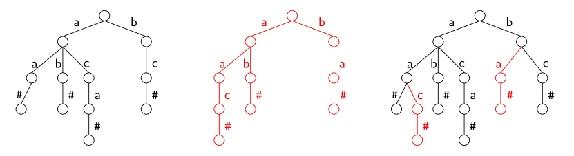
$\mathsf{Last}_{0}$  $\mathsf{L}_{0}$ $\Pi_{0}$ 0 a $\epsilon$ 1 b 0 a a 0 b 1 c 1 # aa 1 # aca 1 c b 1 # ba 1 a ca 1 # cb

$\mathsf{Last}_{1}$  $\mathsf{L}_{1}$ $\Pi_{1}$ 0 a $\epsilon$ 1 b 0 a a 1 b 1 c aa 1 # ab 1 a b 1 # ba 1 # caa

$\mathsf{Last}_{01}$  $\mathsf{L}_{01}$ $\Pi_{01}$ 0 a $\epsilon$ 1 b 0 a a 0 b 1 c 0 # aa 1 c 1 # ab 1 # aca 0 a b 1 c 1 # ba 1 a ca 1 # caa 1 # cb

Figure 6. The trie ${T_{0}}$ containing the strings aa#, ab#, aca#, bc# (left), the trie ${T_{1}}$ containing aac#, ab#, ba# (center) and the trie ${T_{01}}$ containing the union of the two set of strings (right). Below each trie we show the corresponding XBWT representation.

Tries [21] are a fundamental data structure for representing a collection of $k$ distinct strings. A trie consists of a rooted tree in which each edge is labeled with a symbol in the input alphabet, and each string is represented by a path from the root to one of the leaves. To simplify the algorithms, and ensure that no string is the prefix of another one, it is customary to add a special symbol $\mbox{{\#}}\not\in\Sigma$ at the end of each string. Tries for different sets of strings are shown in Figure 6. For any trie node $u$ we write $\mathsf{hgt}(u)$ to denote its height, that is the length of the path from the root to $u$. We define the height of the trie $T$ as the maximum node height $\mathsf{hgt}(T)=\max_{u}\mathsf{hgt}(u)$, and the average height $\mathsf{avehgt}(T)=(\sum_{u}\mathsf{hgt}(u))/|T|$, where $|T|$ denotes the number of trie nodes.

The eXtended Burrows-Wheeler Transform [10, 25, 32] is a generalization of the BWT designed to compactly represent any labeled tree $T$. To define $\mathsf{xbwt}(T)$, to each internal node $w$ we associate the string $\lambda_{w}$ obtained by concatenating the symbols in the edges in the upward path from $w$ to the root of $T$. If $T$ has $n$ internal nodes we have $n$ strings overall; let $\Pi[1,n]$ denote the array containing such strings sorted lexicographically. Note that $\Pi[1]$ is always the empty string corresponding to the root of $T$. For $i=1,\ldots,n$ let $L(i)$ denote the set of symbols labeling the edges exiting from the node corresponding to $\Pi[i]$. We define the array $\mathsf{L}$ as the concatenation of the arrays $L(1),\ldots,L(n)$. If $T$ has $m$ edges (and therefore $m+1$ nodes), it is $|\mathsf{L}|=m$ and $\mathsf{L}$ contains $n-1$ symbols from $\Sigma$ and $m+1-n$ occurrences of #. To keep an explicit representation of the intervals $L(1),\ldots,L(n)$ within $\mathsf{L}$, we define a binary array $\mathsf{Last}[1,m]$ such that $\mathsf{Last}[i]=\mathbf{1}$ iff $\mathsf{L}[i]$ is the last symbol of some interval $L(j)$. See Figure 6 for a complete example.

In [9] it is shown that the two arrays $\mathsf{xbwt}(T)=\langle\mathsf{Last},\mathsf{L}\rangle$ are sufficient to represent $T$, and that if they are enriched with data structures supporting constant time rank and select operations, $\mathsf{xbwt}(T)$ can be used for efficient upward and downward navigation and for substring search in $T$. The fundamental property for efficient navigation and search is that there is an one-to-one correspondence between the symbols in $\mathsf{L}$ different from # and the strings in $\Pi$ different from the empty string. The correspondence is order preserving in the sense that the $i$-th occurrence of symbol $c$ corresponds to the $i$-th string in $\Pi$ starting with $c$. For example, in Figure 6 (right) the third a in $\mathsf{Last}_{01}$ corresponds to the third string in $\Pi_{01}$ starting with a, namely ab. Note that ab is the string associated to the node reached by following the edge associated to the third a in $\mathsf{L}_{01}$.

In this section, we consider the problem of merging two distinct XBWTs. More formally, let ${T_{0}}$ (resp. ${T_{1}}$) denote the trie containing the set of strings $\mathsf{t}_{1},\ldots,\mathsf{t}_{k}$ (resp. $\mathsf{s}_{1},\ldots,\mathsf{s}_{h}$), and let ${T_{01}}$ denote the trie containing the strings in the union $\mathsf{t}_{1}$,…, $\mathsf{t}_{k}$, $\mathsf{s}_{1}$, …, $\mathsf{s}_{h}$ (see Figure 6). Note that ${T_{01}}$ might contain less than $h+k$ strings: if the same string appears in both ${T_{0}}$ and ${T_{1}}$ it will be represented in ${T_{01}}$ only once. Given $\mathsf{xbwt}({T_{0}})=\langle\mathsf{Last}_{0},\mathsf{L}_{0}\rangle$ and $\mathsf{xbwt}({T_{1}})=\langle\mathsf{Last}_{1},\mathsf{L}_{1}\rangle$ we want to compute the XBWT representation of the trie ${T_{01}}$.

We observe that if we had at our disposal the sorted string arrays $\Pi_{0}$ and $\Pi_{1}$, then the construction of $\mathsf{xbwt}({T_{01}})$ could be done as follows: First, we merge lexicographically the strings in $\Pi_{0}$ and $\Pi_{1}$, then we scan the resulting sorted array of strings. During the scan

• if we find a string appearing only once then it corresponds to an internal node belonging to either ${T_{0}}$ or ${T_{1}}$; the labels on the outgoing edges can be simply copied from the appropriate range of $\mathsf{L}_{0}$ or $\mathsf{L}_{1}$.

• if we find two consecutive equal strings they correspond respectively to an internal node in ${T_{0}}$ and to one in ${T_{1}}$. The corresponding node in ${T_{01}}$ has a set of outgoing edges equal to the union of the edges of those nodes in ${T_{0}}$ and ${T_{1}}$: thus, the labels in the outgoing edges are the union of the symbols in the appropriate ranges of $\mathsf{L}_{0}$ and $\mathsf{L}_{1}$.

Although the arrays $\Pi_{0}$ and $\Pi_{1}$ are not available, by properly modifying the H&M algorithm we can compute how their elements would be interleaved by the merge operation. Let ${m_{0}}=|\mathsf{L}_{0}|=|\mathsf{Last}_{0}|$, ${n_{0}}=|\Pi_{0}|$, and similarly ${m_{1}}=|L_{1}|=|\mathsf{Last}_{1}|$, ${n_{1}}=|\Pi_{1}|$. Fig. 7 shows the code for the generic $h$-th iteration of the H&M algorithm adapted for the XBWT. Iteration $h$ computes a binary vector $Z^{(h)}$ containing $n_{0}=|\mathsf{t}_{0}|$ 0’s and $n_{1}=|\mathsf{t}_{1}|$ 1’s and such that the following property holds (compare with Property 2.1)

 

1:Initialize array $F[1,\sigma]$

2:$k_{0}\leftarrow 1$; $k_{1}\leftarrow 1$ $\triangleright$ Init counters for $\mathsf{L}_{0}$ and $\mathsf{L}_{1}$

3:$Z^{(h)}\leftarrow{\bf 0}{\bf 1}$ $\triangleright$ First two entries correspond to $\Pi_{0}[1]=\Pi_{1}[1]=\epsilon$

4:for $k\leftarrow 1$ to $n_{0}+n_{1}$ do

5:     $b\leftarrow Z^{(h-1)}[k]$$\triangleright$ Read bit $b$ from $Z^{(h-1)}$

6:     repeat

7:         $c\leftarrow\mathsf{L}_{b}[k_{b}]$ $\triangleright$ Get symbol from $\mathsf{L}_{0}$ or $\mathsf{L}_{1}$ according to $b$

8:         if $c\neq\mbox{{\#}}$ then $\triangleright$ # is ignored: it is not in $\Pi_{0}$ or $\Pi_{1}$

9:              $j\leftarrow F[c]{\mathsf{+}+}$ $\triangleright$ Get destination for $b$ according to symbol $c$

10:              $Z^{(h)}[j]\leftarrow b$ $\triangleright$ Copy bit $b$ to $Z^{(h)}$

11:         end if

12:         $\ell\leftarrow\mathsf{Last}_{b}[k_{b}{\mathsf{+}+}]$ $\triangleright$ Check if $c$ labels last outgoing edge

13:     until $\ell\neq 1$

14:end for

 

Figure 7. Main loop of algorithm H&M modified to merge XBWTs. Array $F$ is initialized so that $F[c]$ contains the number of occurrences of symbols smaller than $c$ in $\mathsf{L}_{0}$ and $\mathsf{L}_{1}$ plus three, to account for $\Pi_{0}[1]=\Pi_{1}[1]=\epsilon$ which are smaller than any other string.

Property 5.1.

At the end of iteration $h$, for $i=2,\ldots,{n_{0}}$ and $j=2,\ldots{n_{1}}$ the $i$-th 0 precedes the $j$-th 1 in $Z^{(h)}$ if and only if

$$\Pi_{0}[i][1,h]\;\preceq\;\Pi_{1}[j][1,h].$$ (8)

∎

In (8) $\Pi_{0}[i][1,h]$ denotes the length-$h$ prefix of $\Pi_{0}[i]$. If $\Pi_{0}[i]$ has length smaller than $h$ then $\Pi_{0}[i][1,h]=\Pi_{0}[i]$ (and similarly for $\Pi_{1}[j]$). Note that Property 5.1 does not mention the first ${\bf 0}$ and the first ${\bf 1}$ in $Z^{(h)}$: By construction it is $\Pi_{0}[1]=\Pi_{1}[1]=\epsilon$ so we know their lexicographic rank is the smallest possible. Note also that because of Step 3 in Fig. 7, the first ${\bf 0}$ and the first ${\bf 1}$ in $Z^{(h)}$ are always the first two elements of $Z^{(h)}$.

Apart from the first two entries, during iteration $h$ the array $Z^{(h)}$ is logically partitioned into $\sigma$ subarrays, one for each alphabet symbol different from #. If $Occ(c)$ denotes the number of occurrences in $\mathsf{L}_{0}$ and $\mathsf{L}_{1}$ of the symbols smaller than $c$, then the subarray corresponding to $c$ starts at position $Occ(c)+3$. Hence, if $c<c^{\prime}$ the subarray corresponding to $c$ precedes the one corresponding to $c^{\prime}$. Because of how the array $F$ is initialized and updated, we see that every time we read a symbol $c$ from $\mathsf{L}_{0}$ and $\mathsf{L}_{1}$ we write a value in the portion of $Z^{(h)}$ corresponding to $c$, and that each portion is filled sequentially. Armed with these observations, we are ready to establish the correctness of the algorithm in Figure. 7.

Lemma 5.2.

Let $Z^{(0)}={\bf 0}{\bf 1}{\bf 0}^{n_{0}-1}{\bf 1}^{n_{1}-1}$, and let $Z^{(h)}$ be obtained from $Z^{(h-1)}$ by the algorithm in Fig. 7. Then, for $h=0,1,2,\ldots$, the array $Z^{(h)}$ satisfies Property 5.1.

Proof 5.3.

We prove the result by induction. For $h=0$, $\Pi_{0}[i][1,0]=\Pi_{1}[j][1,0]=\epsilon$ so (8) is always true and $Z^{(0)}$ satisfies Property 5.1.

Suppose now $h>0$. To prove the “if” part, let $3\leq v<w\leq{n_{0}}+{n_{1}}$ denote two indexes such that $Z^{(h)}[v]$ is the $i$-th 0 and $Z^{(h)}[w]$ is the $j$-th 1 in $Z^{(h)}$ for some $2\leq i\leq{n_{0}}$ and $2\leq j\leq{n_{1}}$ (it is $v\geq 3$ since $i\geq 2$ and $Z^{(h)}[1,2]={\bf 0}{\bf 1}$). We need to show that (8) holds.

Assume first $\Pi_{0}[i][1]\neq\Pi_{1}[j][1]$. The hypothesis $v<w$ implies $\Pi_{0}[i][1]<\Pi_{1}[j][1]$ hence (3) certainly holds. Assume now $\Pi_{0}[i][1]=\Pi_{1}[j][1]=c$. Let $v^{\prime}$, $w^{\prime}$ denote respectively the values of the main loop variable $k$ in the procedure of Figure 7 when the entries $Z^{(h)}[v]$ and $Z^{(h)}[w]$ are written (hence, during the scanning of $Z^{(h-1)}$). The hypotheses $v<w$ and $\Pi_{0}[i][1]=\Pi_{1}[j][1]$ imply ${v}^{\prime}<{w}^{\prime}$. By construction $Z^{(h-1)}[{v}^{\prime}]=\mathbf{0}$ and $Z^{(h-1)}[{w}^{\prime}]=\mathbf{1}$. Say ${v}^{\prime}$ is the $i^{\prime}$-th 0 in $Z^{(h-1)}$ and ${w}^{\prime}$ is the $j^{\prime}$-th 1 in $Z^{(h-1)}$. By the inductive hypothesis on $Z^{(h-1)}$ we have

$$\Pi_{0}[i^{\prime}][1,h-1]\;\preceq\;\Pi_{1}[j^{\prime}][1,h-1]$$ (9)

(we could have $v^{\prime}=1$ that would imply $i^{\prime}=1$; in that case we cannot apply the inductive hypothesis, but (9) still holds). By the properties of the XBWT we have

$$\Pi_{0}[i][1,h]=c\,\Pi_{0}[i^{\prime}][1,h-1]\qquad\mbox{and}\qquad\Pi_{1}[j][1,h]=c\,\Pi_{1}[j^{\prime}][1,h-1]$$

which combined with (9) gives us (8).

For the “only if” part assume (8) holds for some $i\geq 2$ and $j\geq 2$. We need to prove that in $Z^{(h)}$ the $i$-th 0 precedes the $j$-th 1. If $\Pi_{0}[i][1]\neq\Pi_{1}[j][1]$ the proof is immediate. If $c=\Pi_{0}[i][1]=\Pi_{1}[j][1]$ then

$$\Pi_{0}[i][2,h]\preceq\Pi_{1}[j][2,h].$$

Let $i^{\prime}$ and $j^{\prime}$ be such that $\Pi_{0}[i^{\prime}][1,h-1]=\Pi_{0}[i][2,h]$ and $\Pi_{1}[j^{\prime}][1,h-1]=\Pi_{1}[j][2,h]$. By induction, in $Z^{(h-1)}$ the $i^{\prime}$-th 0 precedes the $j^{\prime}$-th 1 (again we could have $i^{\prime}=1$ and in that case we cannot apply the inductive hypothesis, but the claim still holds).

During iteration $h$, the $i$-th 0 in $Z^{(h)}$ is written to position $v$ when processing the $i^{\prime}$-th 0 of $Z^{(h-1)}$, and the $j$-th 1 in $Z^{(h)}$ is written to position $w$ when processing the $j^{\prime}$-th 1 of $Z^{(h-1)}$. Since in $Z^{(h-1)}$ the $i^{\prime}$-th 0 precedes the $j^{\prime}$-th 1 and since $v$ and $w$ both belongs to the subarray of $Z^{(h)}$ corresponding to the symbol $c$, their relative order does not change and the $i$-th 0 precedes the $j$-th 1 as claimed.∎

As in the original H&M algorithm we stop the merge phase after the first iteration $h$ such that $Z^{(h)}=Z^{(h-1)}$. Since in subsequent iterations we would have $Z^{(g)}=Z^{(h)}$ for any $g>h$, we get that by Property 5.1, $Z^{(h)}$ gives the correct lexicographic merge of $\Pi_{0}$ and $\Pi_{1}$. Note however that the lexicographic order is not sufficient to establish whether two consecutive nodes, say $\Pi_{0}[i]$ and $\Pi_{1}[j]$ have the same upward path and therefore should be merged in a single node of ${T_{01}}$. To this end, we consider the integer array $B$ used in Section 2.1 to mark the starting point of each block. We have shown in Corollary 3.3 that at the end of the original H&M algorithm $B$ contains the LCP values plus one. Indeed, at iteration $h$ the algorithm sets $B[k]=h$ since it “discovers” that the suffixes in $\mathsf{sa}_{01}[k-1]$ and $\mathsf{sa}_{01}[k]$ differ in the $h$-th symbol (hence $\mathsf{lcp}_{01}[k]=h-1$). If we maintain the array $B$ in the XBWT merging algorithm, we get that at the end of the computation if the strings associated to $\Pi_{0}[i]$ and $\Pi_{1}[j]$ are identical then the entry in $B$ corresponding to $\Pi_{1}[j]$ would be zero, since the two strings do not differ in any position. Hence, at the end of the modified H&M algorithm the array $Z^{(h)}$ provides the lexicographic order of the nodes, and the array $B$ the position of the nodes of ${T_{0}}$ and ${T_{1}}$ with the same upward path. We conclude that with a single scan of $Z^{(h)}$ and $B$ we can merge all paths and compute $\mathsf{xbwt}({T_{0}})$. Finally, we observe that instead of $B$ we can use a two-bit array $B_{2}$ as in Sect. 4.2, since we are only interested in determining whether a certain entry is zero, and not in its exact value.

Lemma 5.4.

The modified H&M algorithm computes $\mathsf{xbwt}({T_{01}})$ given $\mathsf{xbwt}({T_{0}})$ and $\mathsf{xbwt}({T_{1}})$ in $\mathcal{O}(|{T_{01}}|\mathsf{hgt}({T_{01}}))$ time and $4n+\mathcal{O}(\log n)$ bits of working space, where $n={n_{0}}+{n_{1}}$.

Proof 5.5.

Each iteration of the merging algorithm takes $\mathcal{O}({m_{0}}+{m_{1}})$ time since it consists of a scan of the arrays $Z^{(h-1)}$, $\mathsf{L}_{0}$, $\mathsf{L}_{1}$, $\mathsf{Last}_{0}$ and $\mathsf{Last}_{1}$. After at most $\mathsf{hgt}({T_{01}})$ iterations the strings in $\Pi_{0}$ and $\Pi_{1}$ are lexicographically sorted and $Z^{(h)}$ no longer changes. The final scan of $Z^{(h)}$ and $B_{2}$ to compute $\mathsf{xbwt}({T_{0}})$ takes $\mathcal{O}({m_{0}}+{m_{1}})$ time. Since $|{T_{01}}|\geq\max({m_{0}},{m_{1}})$ the overall cost is $\mathcal{O}(|{T_{01}}|\mathsf{hgt}({T_{01}}))$ time. The working space of the algorithm, consists of $B_{2}$ and of two instances of the $Z^{(h)}$ array (for the current and the previous iteration), in addition to $\mathcal{O}(\sigma)$ counters (recall that $\sigma$ is assumed to be constant).∎

As for BWT/LCP merging, we now show how to reduce the running time by skipping the portions of $Z^{(h)}$ that no longer change from one iteration to the next. Note that we cannot use monochrome blocks to early terminate XBWT merging. Indeed, from the previous discussion we know that if two strings $\Pi_{0}[i]$ and $\Pi_{1}[j]$ are equal, they will form a non-monochrome block that will never be split.

For this reason we introduce an array $C[1,{n_{0}}+{n_{1}}]$ that, at the beginning of iteration $h$, keeps track of all the strings in $\Pi_{0}$ and $\Pi_{1}$ that have length less than $h$. More precisely, for $i=1,\ldots,{n_{0}}$ (resp. $j=1,\ldots,{n_{1}}$) if the $i$-th 0 (resp. the $j$-th 1) is in position $k$ of $Z^{(h)}$, then $C[k]=\ell>0$ iff the length $|\Pi_{0}[i]|$ (resp. $|\Pi_{1}[j]|$) is equal to $\ell-1$ with $\ell-1<h$. As a consequence, if $C[k]=0$ then the string corresponding to $C[k]$ has length $h$ or more. Note that by Property 5.1 at the beginning of iteration $h$ the algorithm has already determined the lexicographic rank of all the strings in $\Pi_{0}$ and $\Pi_{1}$ of length smaller than $h$. Hence, the entry in $Z^{(h)}[k]$ will not change in successive iterations and will remain associated to the same string from $\Pi_{0}$ or $\Pi_{1}$.

The array $C$ is initialized as $110^{{n_{0}}+{n_{1}}-2}$ since at the beginning of iteration 1 it is $Z^{(h)}={\bf 0}{\bf 1}{\bf 0}^{{n_{0}}-1}{\bf 1}^{{n_{1}}-1}$ and indeed the only strings of length 0 are $\Pi_{0}[0]=\Pi_{1}[0]=\epsilon$. During iteration $h$, we update $C$ adding, immediately after Line 10 in Fig. 7, the line

$$\mathbf{if\ }C[k]=h\mathbf{\ then\ }C[j]\leftarrow h+1\qquad$$

The rationale is that if, during iteration $h-1$ we found out that the string $\alpha$ corresponding to $Z^{(h-1)}[k]$ has length $h-1$ (so we set $C[k]=h$), then the string corresponding to $Z^{(h)}[j]$ is $c\alpha$ and has therefore length $h$.

By the above discussion we see that if at iteration $h$ we write $h+1$ to position $C[j]$, then at iteration $h+1$ we can possibly use $C[j]$ to write $h+2$ in some other position in $C$, but starting from iteration $h+2$ it is no longer necessary to process neither $C[j]$ nor $Z^{(h+2)}[j]$ since they will not affect neither $C$ nor $Z^{(h+3)}$. In other words, during iteration $h$ we can skip all ranges $Z^{(h)}[\ell,m]$ such that $C[\ell,m]$ contains only positive values smaller than $h$. These ranges grown larger and larger as the algorithm proceeds and are handled in the same way as the irrelevant blocks in Gap. Finally, we observe that, using the same techniques as in Section 4.2, we can replace the integer array $C$ with an array $C_{2}$ containing only two bits per entry.

Theorem 5.6.

The modified Gap algorithm computes $\mathsf{xbwt}({T_{01}})$ given $\mathsf{xbwt}({T_{0}})$ and $\mathsf{xbwt}({T_{1}})$ in $\mathcal{O}(|{T_{01}}|\mathsf{avehgt}({T_{01}}))$ time. The working space is $6n+\mathcal{O}(\log n)$ bits, where $n={n_{0}}+{n_{1}}$, plus the space required for handling irrelevant blocks.

Proof 5.7.

The analysis is similar to the one in Theorem 4.6. Here the algorithm executes $\mathsf{hgt}({T_{01}})$ iterations; however, because of irrelevant blocks, iterations have decreasing costs. To bound the overall running time, observe that the cost of each iteration is dominated by the cost of processing the entries in $\mathsf{L}_{0}$ and $\mathsf{L}_{1}$. The generic entry $\mathsf{L}_{0}[i]$ corresponds to a trie node $u_{i}$ with upward path of length $\mathsf{hgt}(u_{i})$. Entry $\mathsf{L}_{0}[i]$ is processed when the Gap algorithm reaches the entry in $Z^{(h)}$ corresponding to the string $\Pi_{1}[i^{\prime}]$ associated to $u_{i}$’s parent. We know that $Z^{(h)}$’s entry corresponding to $\Pi_{1}[i^{\prime}]$ becomes irrelevant after iteration $|\Pi_{1}[i^{\prime}]|+1=\mathsf{hgt}(u_{i})$. Hence, the overall cost of processing $u_{i}$ is $\mathcal{O}(\mathsf{hgt}(u_{i}))$. Summing over all entries in $\mathsf{L}_{0}$ and $\mathsf{L}_{1}$ the total cost is $\mathcal{O}(|{T_{0}}|\mathsf{avehgt}({T_{0}})+|{T_{1}}|\mathsf{avehgt}({T_{1}}))$. The thesis follows observing that $|{T_{01}}|\mathsf{avehgt}({T_{01}})\geq\max\bigl{(}|{T_{0}}|\mathsf{avehgt}({T_{0}}),|{T_{1}}|\mathsf{avehgt}({T_{1}})\bigr{)}$.∎

6. Merging indices for circular patterns

Another well known variant of the BWT is the multistring circular BWT which is defined by sorting the cyclic rotations of the input strings instead of their suffixes. However, to make the transformation reversible, the cyclic rotations have to be sorted according to an order relation, different from the lexicographic order, that we now quickly review.

For any string $\mathsf{t}$, we define the infinite form $\mathsf{t}^{\infty}$ of $\mathsf{t}$ as the infinite length string obtained concatenating $\mathsf{t}$ to itself infinitely many times. Given two strings $\mathsf{t}$ and $\mathsf{s}$ we write $\mathsf{t}\preceq^{\infty}\mathsf{s}$ to denote that $\mathsf{t}^{\infty}\preceq\mathsf{s}^{\infty}$. For example, for $\mathsf{t}=\mathsf{abaa}$ and $\mathsf{s}=\mathsf{aba}$, it is $\mathsf{t}^{\infty}=\mathsf{abaaabaa\cdots}$ and $\mathsf{s}^{\infty}=\mathsf{abaabaaba}\cdots$ so $\mathsf{t}\preceq^{\infty}\mathsf{s}$. Notice that $\mathsf{t}^{\infty}=\mathsf{s}^{\infty}$ does not necessarily imply that $\mathsf{t}=\mathsf{s}{}$. For example, for $\mathsf{t}=\mathsf{ababab}$ and $\mathsf{s}{}=\mathsf{abab}$ it is $\mathsf{t}^{\infty}=\mathsf{s}^{\infty}$. The following lemma, which is a consequence of Fine and Wilf Theorem [36] and a restatement of Proposition 5 in [24], provides an upper bound to the number of comparisons required to establish whether $\mathsf{t}^{\infty}=\mathsf{s}^{\infty}$.

Lemma 6.1.

If $\mathsf{t}^{\infty}\neq\mathsf{s}^{\infty}$ then there exists an index $i\leq|\mathsf{t}|+|\mathsf{s}{}|-\gcd(|\mathsf{t}|,|\mathsf{s}{}|)$ such that $\mathsf{t}^{\infty}[i]\neq\mathsf{s}{}^{\infty}[i]$.∎

A string is primitive if all its cyclic rotations are distinct. The following Lemma is another well known consequence of the Fine and Wilf Theorem.

Lemma 6.2.

If $\mathsf{t}$ and $\mathsf{s}{}$ are primitive, $\mathsf{t}^{\infty}=\mathsf{s}{}^{\infty}$ implies $\mathsf{t}=\mathsf{s}{}$.∎

Let $\mathsf{t}_{0}[1,{n_{0}}],\mathsf{t}_{1}[1,{n_{1}}]$ be two primitive strings and $\mathsf{t}_{01}[1,n]$ their concatenation of length $n={n_{0}}+{n_{1}}$. For $i=1,\ldots,n$, let $\mathsf{rot}_{01}(i)$ define the rotation of substrings $\mathsf{t}_{0}$ and $\mathsf{t}_{1}$ within $\mathsf{t}_{01}$ as follows:

$$\mathsf{rot}_{01}(i)=\begin{cases}\mathsf{t}_{0}[i,{n_{0}}]\mathsf{t}_{0}[1,i-1]&\mbox{if }0<i\leq{n_{0}}\\ \mathsf{t}_{1}[i-{n_{0}},{n_{1}}]\mathsf{t}_{1}[1,i-{n_{0}}-1]&\mbox{if }{n_{0}}<i\leq{n_{0}}+{n_{1}}.\end{cases}$$

For example, if $\mathsf{t}_{0}=\mathsf{abc}$ and $\mathsf{t}_{1}=\mathsf{abbb}$, it is $\mathsf{rot}_{01}(2)=\mathsf{bca}$ and $\mathsf{rot}_{01}(7)=\mathsf{babb}$. The above definition of rotations of substrings can be obviously generalized to a collection of $k$ strings.

In addition to assuming that $\mathsf{t}_{0}$ and $\mathsf{t}_{1}$ are primitive, we assume that $\mathsf{t}_{0}$ is not a rotation of $\mathsf{t}_{1}$. We define the circular Suffix Array of $\mathsf{t}_{0}$ and $\mathsf{t}_{1}$, $\mathsf{csa}_{01}$ as the permutation of $[1,n]$ such that:

$$\mathsf{rot}_{01}(\mathsf{csa}_{01}[i])\;\preceq^{\infty}\;\mathsf{rot}_{01}(\mathsf{csa}_{01}[i+1]).$$ (10)

Note that because of our assumptions and Lemma 6.2, the inequality in (10) is always strict. Finally, the multistring circular Burrows-Wheeler Transform (cBWT) is defined as

$$\mathsf{cbwt}_{01}[i]=\begin{cases}\mathsf{t}_{0}[{n_{0}}]&\mbox{if }\mathsf{csa}_{01}[i]=1\\ \mathsf{t}_{0}[\mathsf{csa}_{01}[i]-1]&\mbox{if }1<\mathsf{csa}_{01}[i]\leq{n_{0}}\\ \mathsf{t}_{1}[{n_{1}}]&\mbox{if }\mathsf{csa}_{01}[i]={n_{0}}+1\\ \mathsf{t}_{1}[\mathsf{csa}_{01}[i]-{n_{0}}-1]&\mbox{if }\mathsf{csa}_{01}[i]>{n_{0}}+1.\end{cases}$$

The above definition given for $\mathsf{t}_{0}$ and $\mathsf{t}_{1}$ can be generalized to any number of strings. The $\preceq^{\infty}$ order and the above multistring circular BWT has been introduced in [24]. In [11] the authors uses a data structure equivalent to a circular BWT to design a compressed permuterm index for prefix/suffix queries. The crucial observation is that if we add a unique symbol # at the end of each string, the same symbol for every string, then searching $\beta\mbox{{\#}}\alpha$ in a circular BWT returns all the strings prefixed by $\alpha$ and suffixed by $\beta$. In [17] Hon et al. use the circular BWT to design a succinct index for circular patterns. Note that Hon et al. in addition to $\mathsf{cbwt}_{01}$ use an additional data structure $\mathsf{length}_{01}$ such that $\mathsf{length}_{01}(i)$ provides the length of the string $\mathsf{t}_{j}$ to which the symbol $\mathsf{cbwt}_{01}[i]$ belongs. Finally, a lightweight algorithm for the construction of the circular BWT has been described in [18]: for a string of length $n$ the proposed algorithm takes $\mathcal{O}(n)$ time and uses $\mathcal{O}(n\log\sigma)$ bits of space.

To simplify our analysis, we preliminary extend the concept of longest common prefix to the $\preceq^{\infty}$ order. For any pair of strings $\mathsf{t},\mathsf{s}{}$ we define

$$\mathsf{cLCP}(\mathsf{t},\mathsf{s}{})=\begin{cases}\mathsf{LCP}(\mathsf{t}^{\infty},\mathsf{s}{}^{\infty})&\mbox{if }\mathsf{t}^{\infty}\neq\mathsf{s}{}^{\infty}\\ |\mathsf{t}|+|\mathsf{s}{}|-\gcd(|\mathsf{t}|,|\mathsf{s}{}|)&\mbox{otherwise}.\end{cases}$$ (11)

Because of Lemma 6.1, $\mathsf{cLCP}(\mathsf{t},\mathsf{s}{})$ generalizes the standard LCP in that it provides the number of comparisons that are necessary in order to establish the $\preceq^{\infty}$ ordering between $\mathsf{t}$, $\mathsf{s}{}$. It is then natural to define for $i=2,\ldots,n$

$$\mathsf{clcp}_{01}[i]=\mathsf{cLCP}(\mathsf{rot}_{01}(\mathsf{csa}_{01}[i-1]),\mathsf{rot}_{01}(\mathsf{csa}_{01}[i]))$$ (12)

and the values

$$\mathsf{maxcLcp}=\max\nolimits_{i}\mathsf{clcp}_{01}[i],\qquad\mathsf{avecLcp}=\bigl{(}\sum\nolimits_{i}\mathsf{clcp}_{01}[i]\bigr{)}/n.$$ (13)

that generalize the standard notions of maximum LCP and average LCP.

Let $\mathsf{cbwt}_{0}$ (resp. $\mathsf{cbwt}_{1}$) denote the circular BWT for the collection of strings $\mathsf{t}_{1},\ldots,\mathsf{t}_{k}$ (resp. $\mathsf{s}_{1},\ldots,\mathsf{s}_{h}$). In this section we consider the problem of computing the circular BWT $\mathsf{cbwt}_{01}$ for the union collection $\mathsf{t}_{1}$,…, $\mathsf{t}_{k}$, $\mathsf{s}_{1}$, …, $\mathsf{s}_{h}$. As we previously observed, we assume that all strings are primitive and that within each input collection no string is the rotation of another. However, we cannot rule out the possibility that some $\mathsf{t}_{i}$ is the rotation of some $\mathsf{s}_{j}$. The merging algorithm should therefore recognize this occurrence and eliminate from the union one of the two strings, say $\mathsf{s}_{j}$. In practice, this means that all symbols of $\mathsf{cbwt}_{1}$ coming from $\mathsf{s}_{j}$ must not be included in $\mathsf{cbwt}_{01}$.

To merge $\mathsf{cbwt}_{0}$ and $\mathsf{cbwt}_{1}$ we need to merge their symbols according to their context. By construction, the context of $\mathsf{cbwt}_{0}[i]$ (resp. $\mathsf{cbwt}_{1}[j]$) is $\mathsf{rot}_{0}(\mathsf{csa}_{0}[i])$ (resp. $\mathsf{rot}_{1}(\mathsf{csa}_{1}[j])$), where $\mathsf{rot}_{0}(\mathsf{csa}_{0}[i])$ is a cyclic rotation of the string $\mathsf{t}_{k}$ to which the symbol $\mathsf{cbwt}_{0}[i]$ belongs (and similarly for $\mathsf{rot}_{1}(\mathsf{csa}_{1}[j])$). Note however, that context must be sorted according to the $\prec^{\infty}$ order; hence $\mathsf{cbwt}_{0}[i]$ should precede $\mathsf{cbwt}_{1}[j]$ in $\mathsf{cbwt}_{01}$ iff $\mathsf{rot}_{0}(\mathsf{csa}_{0}[i])\preceq^{\infty}\mathsf{rot}_{1}(\mathsf{csa}_{1}[j])$. The good news is that the H&M algorithm, as described in Figure 2, when applied to $\mathsf{cbwt}_{0}$ and $\mathsf{cbwt}_{1}$ will sort each symbol according to the $\preceq^{\infty}$ order of its context. Notice that the $\preceq^{\infty}$ order induces a significant difference with respect to the merging of BWTs: indeed, since there are no $’s in $\mathsf{cbwt}_{0}$ and $\mathsf{cbwt}_{1}$ Line 9 is never executed and the destination of each symbol is always determined by its predecessor in the cyclic rotation. More formally, reasoning as in Lemma 2.1, it is possible to prove the following property.

Property 6.3.

For $i=1,\ldots,n_{0}$ and $j=1,\ldots n_{1}$ the $i$-th 0 precedes the $j$-th 1 in $Z^{(h)}$ if and only if

$$\mathsf{rot}_{0}(\mathsf{csa}_{0}[i])^{\infty}[1,h]\;\preceq\;\mathsf{rot}_{1}(\mathsf{csa}_{1}[j])^{\infty}[1,h].$$ (14)

∎

Property 6.3 states that after iteration $h$ the infinite strings $\mathsf{rot}_{0}(\mathsf{csa}_{0}[i])^{\infty}$ and $\mathsf{rot}_{1}(\mathsf{csa}_{1}[j])$ have been sorted according to their length $h$ prefix. As for the original H&M algorithm, as soon as $Z^{(h+1)}=Z^{(h)}$ the $Z^{(\cdot)}$ array will not change in any successive iteration and the merging is complete. By Lemma 6.1 it is $Z^{(h+1)}=Z^{(h)}$ for some $h\leq\mathsf{maxcLcp}$.

Since we do not simply need to sort the context, but also recognize if some string $\mathsf{t}_{i}$ is a rotation of some $\mathsf{s}_{j}$, we make use of the algorithm in Figure 3 which, in addition to $Z^{(h)}$, also computes the integer array $B$ that marks the boundaries of the groups of all rotations whose infinite form have a common prefix of length $h$. We can prove a result analogous to Lemma 3.1 replacing the LCP between suffixes ($\mathsf{lcp}_{01}$) with the LCP between the infinite strings $\mathsf{rot}_{b}(\mathsf{csa}_{b}[i])^{\infty}$ (that is $\mathsf{clcp}_{01}$). After iteration $h=\mathsf{maxcLcp}$ all distinct rotations have been sorted according to the $\preceq^{\infty}$ order; thus an entry $B[k]=0$ denotes two rotations $\mathsf{rot}_{0}(\mathsf{csa}_{0}[i])^{\infty}$ and $\mathsf{rot}_{1}(\mathsf{csa}_{1}[j])^{\infty}$ which have a common prefix of length $\mathsf{maxcLcp}$. By Lemma 6.1 it is $\mathsf{rot}_{0}(\mathsf{csa}_{0}[i])^{\infty}=\mathsf{rot}_{1}(\mathsf{csa}_{1}[j])^{\infty}$ and by Lemma 6.2 $\mathsf{rot}_{0}(\mathsf{csa}_{0}[i])=\mathsf{rot}_{1}(\mathsf{csa}_{1}[j])$. The two rotations are therefore identical and the symbol $\mathsf{cbwt}_{1}[j]$ should not be included in $\mathsf{cbwt}_{01}$.

Summing up, to merge $\mathsf{cbwt}_{0}$ and $\mathsf{cbwt}_{1}$ we execute the procedure of Figure 3 until both $Z^{(h)}$ and $B$ do not change. Then, we compute $\mathsf{cbwt}_{01}$ by merging $\mathsf{cbwt}_{0}$ and $\mathsf{cbwt}_{1}$ according to $Z^{(h)}$, discarding those symbols corresponding to zero entries in $B$. The number of iterations will be at most $\mathsf{maxcLcp}$. In addition, since we are only interested in zero/nonzero entries, instead of $B$ we can use a 2-bit array $B_{2}$ as in Section 4.2. Reasoning as for Lemma 3.5, setting $n={n_{0}}+{n_{1}}$ we get the following result.

Lemma 6.4.

The modified H&M algorithm computes $\mathsf{cbwt}_{01}$ given $\mathsf{cbwt}_{0}$ and $\mathsf{cbwt}_{1}$ in $\mathcal{O}(n\,\mathsf{maxcLcp})$ time and $4n+\mathcal{O}(\log n)$ bits of working space.∎

As we have done in the previous sections, we now show how to reduce the running time of the merging algorithm by avoiding to re-process the blocks of $Z^{(h-1)}$ that have become irrelevant for the computation of the new bitarray $Z^{(h)}$. Reasoning as in Section 4 we observe that monochrome blocks, i.e. blocks containing entries only from $\mathsf{cbwt}_{0}$ or $\mathsf{cbwt}_{1}$, after having been processed once, become irrelevant and can be skipped in successive iterations. Note however, that whenever $\mathsf{rot}_{0}(\mathsf{csa}_{0}[i])^{\infty}=\mathsf{rot}_{1}(\mathsf{csa}_{1}[j])^{\infty}$ these two entries will always belong to the same block. To handle this case we first assume $\mathsf{cbwt}_{01}$ is to be used as a compressed index for circular patterns [17] and we later consider the case in which $\mathsf{cbwt}_{01}$ is to be used for a compressed permuterm index.

6.1. Compressed indices of circular patterns

In this setting, $\mathsf{cbwt}_{01}$ is to be used as a compressed index for circular patterns and therefore we have access to the $\mathsf{length}_{0}$ and $\mathsf{length}_{1}$ data structures providing the length of each rotation. Under this assumption we modify the Gap algorithm described in Section 4 as follows: in addition to skipping monotone blocks, every time there is a size-2 non monochrome block containing, say $\mathsf{cbwt}_{0}[i]$ and $\mathsf{cbwt}_{1}[j]$, we mark it as quasi-irrelevant and compute $\ell_{ij}=|\mathsf{length}_{0}(i)|+|\mathsf{length}_{1}(j)|-\gcd(|\mathsf{length}_{0}(i)|,|\mathsf{length}_{1}(j)|)$. As soon as this block is split or we reach iteration $\ell_{ij}$ the block becomes irrelevant and is skipped in successive iterations. As in the original Gap algorithm, the computation stops when all blocks have become irrelevant.

For simplicity, in the next theorem we assume that the access to the data structures $\mathsf{length}_{0}$ and $\mathsf{length}_{1}$ takes constant time. If not, and random access to the individual lengths takes $\mathcal{O}(\rho)$ time, the overall cost of the algorithm is increased by $\mathcal{O}(({n_{0}}+{n_{1}})\rho)$ since each length is computed at most once.

Theorem 6.5.

The modified Gap algorithm computes $\langle\mathsf{cbwt}_{01},\mathsf{length}_{01}\rangle$ given $\langle\mathsf{cbwt}_{0},\mathsf{length}_{0}\rangle$ and $\langle\mathsf{cbwt}_{1},\mathsf{length}_{1}\rangle$ in $\mathcal{O}(n\;\mathsf{avecLcp})$ time, where $n={n_{0}}+{n_{1}}$. The working space is $2n+\mathcal{O}(\log n)$ bits plus the space required for handling (quasi-)irrelevant blocks.

Proof 6.6.

If $\mathsf{rot}_{01}(\mathsf{csa}_{01}[k])$ is different from any other rotation, by definitions (11) and (12) after at most $\max(\mathsf{clcp}_{01}[k],\mathsf{clcp}_{01}[k+1])$ iterations it will be in a monochrome (possibly singleton) block. If instead $\mathsf{rot}_{01}(\mathsf{csa}_{01}[k])$ is identical to another rotation, which can only be either $\mathsf{rot}_{01}(\mathsf{csa}_{01}[k-1])$ or $\mathsf{rot}_{01}(\mathsf{csa}_{01}[k+1])$, then after at most

$$\max(\mathsf{clcp}_{01}[k-1],\mathsf{clcp}_{01}[k],\mathsf{clcp}_{01}[k+1],\mathsf{clcp}_{01}[k+2])$$ (15)

iterations it will be in a size-2 non-monochrome block together with its identical rotation. In either case, the block containing $\mathsf{rot}_{01}(\mathsf{csa}_{01}[k])$ will become irrelevant and it will be no longer processed in successive iterations. Hence, the overall cost of handling $\mathsf{rot}_{01}(\mathsf{csa}_{01}[k])$ over all iterations is proportional to (15), and the overall cost of handling all rotations is bounded by $\mathcal{O}(n\;\mathsf{avecLcp})$ as claimed. Note that the final bitarray $Z^{(h)}$ describes also how $\mathsf{length}_{0}$ and $\mathsf{length}_{1}$ must be interleaved to get $\mathsf{length}_{01}$.∎

6.2. Compressed permuterm indices

Finally, we consider the case in which $\mathsf{cbwt}_{01}$ is to be used as the core of a compressed permuterm index [11]. In this case we do not have the $\mathsf{length}_{0}$ and $\mathsf{length}_{1}$ data structures, but each string in the collection is terminated by a unique # symbol. In this case, to recognize whether a size-2 non-monochrome block contains two identical rotations, we make use of the following lemma.

Lemma 6.7.

Let $\mathsf{t}$ and $\mathsf{s}{}$ denote two strings each one containing a single occurrence of the symbol #. If for some $h>0$ it is  ${\mathsf{t}}^{\infty}[1,h]={\mathsf{s}{}}^{\infty}[1,h]$  and ${\mathsf{t}}^{\infty}[1,h]$ contains two occurrences of #, then $\mathsf{t}=\mathsf{s}{}$.

Proof 6.8.

Let $\delta$ denote the distance between the two occurrences of # in ${\mathsf{t}}^{\infty}[1,h]$. Since $\mathsf{t}$ contains a single #, we have $\mathsf{t}={\mathsf{t}}^{\infty}[1,\delta]={\mathsf{s}{}}^{\infty}[1,\delta]=\mathsf{s}{}$.∎

The above lemma suggests to design a #Gap algorithm to merge compressed permuterm indices in which the arrays $Z^{(\cdot)}$ are arrays of pairs so that they keep track also of the number of # in each prefix. In the following $Z^{(h)}[k]=\langle b,m\rangle$ means that the $k$-th rotation belongs to $\mathsf{csa}_{b}$, and among the first $h$ symbols of the infinite form of that rotation there are exactly $m$ occurrences of #. Formally, for $h=0,1,2,\ldots$ the array $Z^{(h)}$ satisfies the following property.

Property 6.9.

At the end of iteration $h$ of #Gap Property 6.3 holds and if $Z^{(h)}[k]=\langle b,m\rangle$ is the $i$-th $b$ in $Z^{(h)}$ then $\mathsf{rot}_{b}(\mathsf{csa}_{b}[i])^{\infty}[1,h]$ contains exactly $m$ copies of symbol #.∎

Initially we set $Z^{(0)}=\langle\mathbf{0},0\rangle^{n_{0}}\langle\mathbf{1},0\rangle^{n_{1}}$ which clearly satisfies Property 6.9. At each iteration #Gap reads $Z^{(h-1)}$ and updates $Z^{(h)}$ using Lines 7–15 below instead of Lines 7–14 of Figure 3:

7:$\langle b,m\rangle\leftarrow Z^{(h-1)}[k]$

8:$c\leftarrow\mathsf{bwt}_{b}[k_{b}{\mathsf{+}+}]$ $\triangleright$ Get $c$ according to $b$

9:$\vdots$

14:$\mathbf{if\ }c=\mbox{{\#}}\mathbf{\ then\ }m\leftarrow m+1$$\triangleright$ Update number of #

15:$Z^{(h)}[j]\leftarrow\langle b,m\rangle$

Reasoning as in the previous sections, one can prove by induction that with this modification the array $Z^{(h)}$ computed by #Gap satisfies Property 6.9. In the #Gap algorithm a block becomes irrelevant when it is monochrome or it is a size-2 non-monochrome block $Z^{(h)}[k,k+1]$ such that $Z^{(h)}[k]=\langle\mathbf{0},2\rangle$ and $Z^{(h)}[k+1]=\langle\mathbf{1},2\rangle$. By Lemma 6.7 such block corresponds to two identical rotations $\mathsf{rot}_{0}(\mathsf{csa}_{0}[i])=\mathsf{rot}_{1}(\mathsf{csa}_{1}[j])$ and after being processed a final time it can be ignored in successive iterations.

In the practical implementation of the #Gap algorithm, instead of maintaining the pairs $\langle b,m\rangle$, we maintain two bit arrays $Z^{(h-1)}$, $Z^{(h)}$ as in Gap, and an additional 2-bit array $C$ containing the second component of the pairs. For such array $C$ two bits per entry are sufficient since the values stored in each entry $C[k]$ never decrease and they are no longer updated when they reach the value 2.

Theorem 6.10.

The #Gap algorithm merges two compressed permuterm indices $\mathsf{cbwt}_{0}$ and $\mathsf{cbwt}_{1}$ in $\mathcal{O}(n\;\mathsf{avecLcp})$ time, where $n={n_{0}}+{n_{1}}$. The working space is $6n+\mathcal{O}(\log n)$ bits plus the space required for handling irrelevant blocks.

Proof 6.11.

We reason as in the proof of Theorem 6.5 except that if $\mathsf{rot}_{01}(\mathsf{csa}_{01}[k])=\mathsf{rot}_{01}(\mathsf{csa}_{01}[k+1])$ we are guaranteed that the corresponding size-2 block will become irrelevant only after iteration $h=2\,|\mathsf{rot}_{01}(\mathsf{csa}_{01}[k])|=2\,\mathsf{clcp}_{01}[k+1]$. Hence, the cost of handling $\mathsf{rot}_{01}(\mathsf{csa}_{01}[k])$ is still proportional to (15) and the overall cost of the algorithm is $\mathcal{O}(n\;\mathsf{avecLcp})$ time. The space usage is the same as in Theorem 6.5, except for the $2n$ additional bits for the $C$ array.∎

References

- [1] Djamal Belazzougui. Linear time construction of compressed text indices in compact space. In STOC, pages 148–193. ACM, 2014.
- [2] Christina Boucher, Alexander Bowe, Travis Gagie, Simon J. Puglisi, and Kunihiko Sadakane. Variable-order de Bruijn graphs. In DCC, pages 383–392. IEEE, 2015.
- [3] Alexander Bowe, Taku Onodera, Kunihiko Sadakane, and Tetsuo Shibuya. Succinct de Bruijn graphs. In WABI, volume 7534 of Lecture Notes in Computer Science, pages 225–235. Springer, 2012.
- [4] M. Burrows and D. Wheeler. A block-sorting lossless data compression algorithm. Technical Report 124, Digital Equipment Corporation, 1994.
- [5] Anthony J. Cox, Fabio Garofalo, Giovanna Rosone, and Marinella Sciortino. Lightweight LCP construction for very large collections of strings. J. Discrete Algorithms, 37:17–33, 2016.
- [6] Lavinia Egidi, Felipe Alves Louza, and Giovanni Manzini. Space-efficient merging of succinct de Bruijn graphs. CoRR, 2019. URL: https://arxiv.org/abs/1902.02889.
- [7] Lavinia Egidi, Felipe Alves Louza, Giovanni Manzini, and Guilherme P. Telles. External memory BWT and LCP computation for sequence collections with applications. In WABI, volume 113 of LIPIcs, pages 10:1–10:14. Schloss Dagstuhl - Leibniz-Zentrum fuer Informatik, 2018.
- [8] Lavinia Egidi and Giovanni Manzini. Lightweight BWT and LCP merging via the gap algorithm. In SPIRE, volume 10508 of Lecture Notes in Computer Science, pages 176–190. Springer, 2017.
- [9] P. Ferragina, F. Luccio, G. Manzini, and S. Muthukrishnan. Structuring labeled trees for optimal succinctness, and beyond. In Proc. 46th IEEE Symposium on Foundations of Computer Science (FOCS), pages 184–193, 2005.
- [10] Paolo Ferragina, Fabrizio Luccio, Giovanni Manzini, and S. Muthukrishnan. Compressing and indexing labeled trees, with applications. J. ACM, 57(1):4:1–4:33, 2009.
- [11] Paolo Ferragina and Rossano Venturini. The compressed permuterm index. ACM Trans. Algorithms, 7(1):10:1–10:21, 2010.
- [12] J. Fuentes-Sepúlveda, G. Navarro, and Y. Nekrich. Space-efficient computation of the Burrows-Wheeler Transform. In Proc. 29th Data Compression Conference (DCC), 2019. To appear.
- [13] Travis Gagie, Giovanni Manzini, and Jouni Sirén. Wheeler graphs: A framework for bwt-based data structures. Theor. Comput. Sci., 698:67–78, 2017.
- [14] Simon Gog and Enno Ohlebusch. Compressed suffix trees: Efficient computation and storage of LCP-values. ACM Journal of Experimental Algorithmics, 18, 2013. doi:10.1145/2444016.2461327.
- [15] James Holt and Leonard McMillan. Constructing Burrows-Wheeler transforms of large string collections via merging. In BCB, pages 464–471. ACM, 2014.
- [16] James Holt and Leonard McMillan. Merging of multi-string BWTs with applications. Bioinformatics, 30(24):3524–3531, 2014.
- [17] W.-K. Hon, C.-H. Lu, R. Shah, and S.V. Thankachan. Succinct indexes for circular patterns. In Algorithms and Computation - 22nd International Symposium, ISAAC 2011, Yokohama, Japan, December 5-8, 2011. Proceedings, pages 673–682, 2011. doi:10.1007/978-3-642-25591-5_69.
- [18] Wing-Kai Hon, Tsung-Han Ku, Chen-Hua Lu, Rahul Shah, and Sharma V. Thankachan. Efficient algorithm for circular burrows-wheeler transform. In CPM, volume 7354 of Lecture Notes in Computer Science, pages 257–268. Springer, 2012.
- [19] J. Kärkkäinen, G. Manzini, and S. Puglisi. Permuted longest-common-prefix array. In Proc. 20th Symposium on Combinatorial Pattern Matching (CPM), pages 181–192. Springer-Verlag, LNCS n. 5577, 2009.
- [20] Juha Kärkkäinen and Dominik Kempa. LCP array construction in external memory. ACM Journal of Experimental Algorithmics, 21(1):1.7:1–1.7:22, 2016.
- [21] D. E. Knuth. Sorting and Searching, volume 3 of The Art of Computer Programming. Addison-Wesley, Reading, MA, USA, second edition, 1998.
- [22] Martine Léonard, Laurent Mouchard, and Mikaël Salson. On the number of elements to reorder when updating a suffix array. J. Discrete Algorithms, 11:87–99, 2012. doi:10.1016/j.jda.2011.01.002.
- [23] Felipe Alves Louza, Simon Gog, and Guilherme P. Telles. Induced suffix sorting for string collections. In DCC, pages 43–52. IEEE, 2016.
- [24] Sabrina Mantaci, Antonio Restivo, Giovanna Rosone, and Marinella Sciortino. An extension of the Burrows-Wheeler transform. Theor. Comput. Sci., 387(3):298–312, 2007.
- [25] Giovanni Manzini. XBWT tricks. In SPIRE, volume 9954 of Lecture Notes in Computer Science, pages 80–92, 2016.
- [26] Martin D. Muggli and Christina Boucher. Succinct de Bruijn graph construction for massive populations through space-efficient merging. bioRxiv, 2017. doi:10.1101/229641.
- [27] Martin D. Muggli, Alexander Bowe, Noelle R. Noyes, Paul S. Morley, Keith E. Belk, Robert Raymond, Travis Gagie, Simon J. Puglisi, and Christina Boucher. Succinct colored de Bruijn graphs. Bioinformatics, 33(20):3181–3187, 2017.
- [28] J. Ian Munro, Gonzalo Navarro, and Yakov Nekrich. Space-efficient construction of compressed indexes in deterministic linear time. In SODA, pages 408–424. SIAM, 2017.
- [29] Joong Chae Na, Hyunjoon Kim, Seunghwan Min, Heejin Park, Thierry Lecroq, Martine Léonard, Laurent Mouchard, and Kunsoo Park. FM-index of alignment with gaps. Theoretical Computer Science, 710:148–157, feb 2018. doi:10.1016/j.tcs.2017.02.020.
- [30] Joong Chae Na, Hyunjoon Kim, Heejin Park, Thierry Lecroq, Martine Léonard, Laurent Mouchard, and Kunsoo Park. FM-index of alignment: A compressed index for similar strings. Theoretical Computer Science, 638:159–170, 2016.
- [31] G. Navarro and V. Mäkinen. Compressed full-text indexes. ACM Computing Surveys, 39(1), 2007.
- [32] Enno Ohlebusch, Stefan Stauß, and Uwe Baier. Trickier XBWT tricks. In SPIRE, volume 11147 of Lecture Notes in Computer Science, pages 325–333. Springer, 2018.
- [33] Jouni Sirén. Compressed suffix arrays for massive data. In Proc. 16th Int. Symp. on String Processing and Information Retrieval (SPIRE ’09), pages 63–74. Springer Verlag LNCS n. 5721, 2009.
- [34] Jouni Sirén. Burrows-Wheeler transform for Terabases. In IEEE Data Compression Conference (DCC), pages 211–220, 2016.
- [35] Jouni Sirén. Indexing variation graphs. In Proc. 19th Meeting on Algorithm Engineering and Experiments (ALENEX ’17), pages 13–27. SIAM, 2017.
- [36] H.S. Wilf and N.J. Fine. Uniqueness theorem for periodic functions. Proc. Amer. Math. Soc., 16:109–114, 1965.