Cheung, Simchi-Levi, and Zhu

Hedging the Drift: Learning to Optimize under Non-Stationarity

Hedging the Drift: Learning to Optimize under Non-Stationarity

Wang Chi Cheung Department of Industrial Systems Engineering and Management, National University of Singapore isecwc@nus.edu.sg David Simchi-Levi Institute for Data, Systems, and Society, Massachusetts Institute of Technology, Cambridge, MA 02139, dslevi@mit.edu Ruihao Zhu Institute for Data, Systems, and Society, Massachusetts Institute of Technology, Cambridge, MA 02139, rzhu@mit.edu

We introduce data-driven decision-making algorithms that achieve state-of-the-art dynamic regret bounds for a collection of non-stationary stochastic bandit settings. These settings capture applications such as advertisement allocation, dynamic pricing, and traffic network routing in changing environments. We show how the difficulty posed by the (unknown a priori and possibly adversarial) non-stationarity can be overcome by an unconventional marriage between stochastic and adversarial bandit learning algorithms. Beginning with the linear bandit setting, we design and analyze a sliding window-upper confidence bound algorithm that achieves the optimal dynamic regret bound when the underlying variation budget is known. This budget quantifies the total amount of temporal variation of the latent environments. Boosted by the novel Bandit-over-Bandit framework that adapts to the latent changes, our algorithm can further enjoy nearly optimal dynamic regret bounds in a (surprisingly) parameter-free manner. We extend our results to other related bandit problems, namely the multi-armed bandit, generalized linear bandit, and combinatorial semi-bandit settings, which model a variety of operations research applications. In addition to the classical exploration-exploitation trade-off, our algorithms leverage the power of the “forgetting principle” in the learning processes, which is vital in changing environments. Extensive numerical experiments with synthetic datasets and a dataset of an online auto-loan company demonstrate that our proposed algorithms achieve superior performance compared to existing algorithms.

data-driven decision-making, non-stationary bandit optimization, parameter-free algorithm

1 Introduction

Consider the following general decision-making framework: a decision-maker (DM) interacts with a multi-armed bandit (MAB) system by picking actions one at a time sequentially. Upon selecting an action, she instantly receives a reward drawn randomly from a probability distribution tied to this action. The goal of the DM is to maximize her cumulative rewards. However, she faces the following challenges:

• Uncertainty: the reward distribution of each action is initially not known to the DM. She has to estimate the underlying reward distributions via interacting with the environment.

• Non-Stationarity: the reward distributions can evolve over time.

• Partial/Bandit Feedback: the DM can only observe the random reward of the selected action each time, while the rewards of the unchosen actions are not observed.

Many applications naturally fall into this non-stationary MAB framework. For instance, with a linear reward model, which will also be the main focus of this paper, we can cast the problems of dynamic pricing (Keskin and Zeevi 2014, 2016), advertisement allocation (Li et al. 2010, Chu et al. 2011) in dynamic and evolving environments into the above decision-making framework. This framework also finds applications in traffic network routing (Gai et al. 2012, Kveton et al. 2015).

Example 1.1 (Dynamic Pricing)

In the classical setup of dynamic pricing (Keskin and Zeevi 2014, 2016), a seller decides dynamically the prices of a product for a sequence of incoming customers with the hope to maximize the cumulative revenue. Beginning with an unknown demand function that represents the customers’ sensitivity towards price changes, the DM only observes the purchase decision (e.g., buy/not buy or purchase quantities) of each customer under the corresponding posted price. Moreover, the demand function can evolve over time due to unexpected events. For example, after the announcement of the COVID-19 pandemic on 11 March 2020 (World Health Organization (2020) WHO), the demand for daily essentials and shelf-stable foods increased suddenly (Becdach et al. 2020).

Example 1.2 (Advertisement Allocation)

An online platform allocates advertisements (ads) to a sequence of users. For each arriving user, the platform has to deliver an ad to her, and only observes the response to her displayed ad. The platform has full access to the features of the ads and the users. Following (Li et al. 2010, Chu et al. 2011), we could assume that a user’s click behavior towards an ad, or simply the click through rate (CTR) of this ad by a particular user, follows a probability distribution governed by a common, but initially unknown, response function of the features. The platform’s goal is to maximize the total number of clicks. However, the unknown response function can change over time. For instance, if it is around the time when Apple releases a new iPhone model, one can expect that the popularity of an Apple’s ad grows.

Example 1.3 (Traffic Network Routing)

A navigation service provider has to iteratively offer route planning services to drivers from an origin to a destination through a traffic network with initially unknown random delay on each road. For each driver, the provider could only see the delays of the roads traversed by this driver, but not the other roads’. Moreover, the delay distributions could change over time as the roads are also shared by other traffics (i.e., those not using this navigation service). The provider wants to minimize the cumulative delays throughout the course of vehicle routing.

Evidently, the DM faces a trilemma among exploration, exploitation as well as adaptation to changes. On one hand, the DM wishes to exploit, and to select the action with the best historical performances to earn as much reward as possible. On the other hand, she wants to explore other actions to get a more accurate estimation of the reward distributions. The changing environment makes the exploration-exploitation trade-off even more delicate. Indeed, past observations could become obsolete due to the changes in the environment, and the DM needs to explore for changes and refrain from exploiting possibly outdated observations.

We focus on resolving this trilemma in various MAB problems. Traditionally, most MAB problems are studied in the stochastic (Auer et al. 2002b) and adversarial (Auer et al. 2002a) environments. In the former, the uncertain model is static, and each feedback is corrupted by a mean zero random noise. The DM aims at estimating the latent static environment using historical data and converging to the optimum, which is achieved by a static strategy that selects a single action throughout. In the latter, the model is not only uncertain, but also dynamically changed by an adversary. While the DM strives to hedge against the changes, it is generally impossible to achieve the optimum. Hence, existing research also focuses on competing favorably in comparison to a static strategy.

Unfortunately, strategies for the stochastic environments can quickly deteriorate under non-stationarity as historical data might “expire”, while the permission of a confronting adversary in the adversarial settings could be too pessimistic. Starting from (Besbes et al. 2014, 2015), a stream of research works (see Section 2) focuses on MAB problems in a drifting environment, which is a hybrid of a stochastic and an adversarial environment. Although the environment can be dynamically and adversarially changed, the total changes (quantified by a suitable metric) in a $T$-round problem is upper bounded by $B_{T}~{}(=\Theta(T^{\rho})\text{ for some }\rho\in(0,1))$, the variation budget (Besbes et al. 2014, 2015), and the feedback is corrupted by an additive mean zero random noise. The aim is to minimize the dynamic regret (Besbes et al. 2014), which is the optimality gap compared to the sequence of (possibly dynamically changing) optimal decisions, by simultaneously estimating the current environment and hedging against future changes every round. The framework of (Besbes et al. 2014, 2015) enable us to compete against the so-called dynamic comparator. Most of the existing works for non-stationary bandits have focused on the the relatively ideal case in which $B_{T}$ is known. In practice, however, $B_{T}$ is often not available ahead as it is a quantity that requires knowledge of future information. Though some efforts have been made towards this direction (Karnin and Anava 2016, Luo et al. 2018), the design of algorithms with low dynamic regret when $B_{T}$ is unknown remains largely a challenging problem.

In this paper, we design and analyze a novel algorithmic framework for bandit problems in drifting environments. We begin by demonstrating our results via the lens of the linear bandit model, and then we demonstrate the generality of our framework on related MAB models. Our main contributions can be summarized as follows.

• When the variation budget $B_{T}$ is known, we provide a lower bound on the dynamic regret incurred by any non-anticipatory policy. In complement, we develop a tuned Sliding Window Upper-Confidence-Bound (SW-UCB) algorithm with a matching dynamic regret upper bound, up to multiplicative logarithmic factors.

• When $B_{T}$ is unknown, we propose a novel Bandit-over-Bandit (BOB) framework that tunes the window size of the SW-UCB algorithm adaptively. When the amount of non-stationarity is above a certain threshold (that depends on $B_{T},T$), the BOB algorithm achieves the optimal dynamic regret bound. Otherwise, it still obtains a dynamic regret bound sublinear in $T$. While the optimal dynamic regret bound is not achieved in the latter case, the resulting dynamic regret bound is better than the state-of-the-art in prior literature.

• Our algorithm design and analysis shed light on the fine balance among exploration, exploitation and adaptation to changes in dynamic learning environments. We rigorously incorporate the “forgetting principle” (Garivier and Moulines 2011) into the Optimism-in-Face-of-Uncertainty principle (Auer et al. 2002b, Abbasi-Yadkori et al. 2011), by demonstrating that the DM can enjoy an optimal dynamic regret bound if she keeps disposing of sufficiently old observations. We also provide a rate of disposal that leads to the optimality.

• Finally, we point out that a preliminary version of this paper appears in the $22^{\text{nd}}$ International Conference on Artificial Intelligence and Statistics (AISTATS 2019) (Cheung et al. 2019), and the current paper provides significant additional contributions in three directions. First, when $B_{T}$ is unknown, the current version provides a substantially refined design and analysis of the BOB algorithm for the linear bandit model, resulting in an improved dynamic regret bound (i.e., Theorem 7.3 of Section 7) compared to Theorem 4 of (Cheung et al. 2019). Second, unlike (Cheung et al. 2019), which only focuses on the linear bandit model, in the current paper we extend our approach, in Section 8, to several related bandit settings, including multi-armed bandits, generalized linear bandits, and combinatorial semi-bandits. These extensions capture many important operations research applications, such as the three examples highlighted in the introduction. Third, we conduct numerical experiments using a new synthetic dataset to evaluate our algorithms in piecewise-linear environments for both 2-armed bandit and linear bandit settings. We also study the performances of our algorithms in a case of dynamic pricing under the SARS epidemic with a real world auto-loan dataset. Both of these experiments extend significantly beyond the simple drifting 2-armed bandit experiments in the AISTATS version.

The rest of the paper is organized as follows. In Section 2, we review existing MAB works in stationary and non-stationary environments. In Section 3, we formulate the non-stationary linear bandit model. In Section 4, we establish a minimax lower bound on the dynamic regret. In Section 5, we describe the sliding window estimator for parameter estimation under non-stationarity. In Section 6, we develop the sliding window-upper confidence bound algorithm with optimal dynamic regret (when the amount of non-stationarity is known ahead). In Section 7, we introduce the novel Bandit-over-Bandit framework with nearly optimal dynamic regret. In Section 8, we demonstrate the generality of the established results by applying them to related bandit settings, namely the multi-armed bandit, generalized linear bandit, and combinatorial semi-bandit settings. In Section 9, we conduct extensive numerical experiments with both synthetic and CPRM-12-001: on-line auto lending datasets to show the superior empirical performances of our algorithms. In Section 10, we conclude our paper.

2 Related Works

2.1 Stationary and Adversarial Bandits

MAB problems with stochastic and adversarial environments are extensively studied, as surveyed in (Bubeck and Cesa-Bianchi 2012, Lattimore and Szepesvári 2018). To model inter-dependence among different arms, models for linear bandits in stochastic environments have been studied. In (Auer 2002, Dani et al. 2008, Rusmevichientong and Tsitsiklis 2010, Chu et al. 2011, Abbasi-Yadkori et al. 2011), UCB type algorithms for stochastic linear bandits were studied, and the authors of (Abbasi-Yadkori et al. 2011) provided the tightest regret analysis for algorithms of this kind. The authors of (Russo and Van Roy 2014, Agrawal and Goyal 2013, Abeille and Lazaric 2017) proposed Thompson sampling algorithms for this setting to bypass the high computational complexity of the UCB type algorithms.

2.2 Bandits in Drifting Environments

Departing from purely stochastic or adversarial settings, Besbes et al. (Besbes et al. 2014, 2015) laid down the foundation of bandit in drifting environments, and considered the $K$-armed bandit setting. They achieved the tight dynamic regret bound $\tilde{O}((KB_{T})^{1/3}T^{2/3})$ by restarting the EXP3 algorithm (Auer et al. 2002a) periodically when $B_{T}$ is known. Wei et al. (2016) provided refined regret bounds based on empirical variance estimation, assuming the knowledge of $B_{T}$. Wei and Srivastava (2018) analyzed the sliding window upper confidence bound algorithm for the $K$-armed MAB with known $B_{T}$ setting. Subsequently, Karnin and Anava (2016) considered the setting without knowing $B_{T}$ and $K=2$, and achieved a dynamic regret bound of $\widetilde{O}(B_{T}^{9/50}T^{41/50}+T^{77/100})$ with a change point detection type technique. In a recent work, Luo et al. (2018) generalized this change point detection type technique to the $K$-armed contextual bandits in drifting environments, and in particular demonstrated an improved bound $\widetilde{O}(KB_{T}^{1/5}T^{4/5})$ for the $K$-armed bandit problem in drifting environments when $B_{T}$ is not known. Keskin and Zeevi (2016) considered a dynamic pricing problem in a drifting environment with 2-dimensional linear demands. Assuming a known variation budget $B_{T},$ they proved an $\Omega(B_{T}^{1/3}T^{2/3})$ dynamic regret lower bound and proposed a matching algorithm by properly discounting historical observations (this includes sliding-window estimation as a special case). When $B_{T}$ is not known, their algorithm achieves $\tilde{O}(B_{T}T^{2/3})$ dynamic regret bound. Finally, various online problems with full feedback in drifting environments were studied in (Chiang et al. 2012, Besbes et al. 2015, Jadbabaie et al. 2015).

	Known $B_{T}$	Unknown $B_{T}$
(Besbes et al. 2015)	$\widetilde{O}\left(B_{T}^{{1}/{3}}T^{{2}/{3}}\right)$	$\widetilde{O}\left(B_{T}T^{{2}/{3}}\right)$
(Karnin and Anava 2016)	$\widetilde{O}\left(B_{T}^{9/50}T^{41/50}+T^{77/100}\right)$	$\widetilde{O}\left(B_{T}^{9/50}T^{41/50}+T^{77/100}\right)$
(Luo et al. 2018)	$\widetilde{O}\left(B_{T}^{{1}/{3}}T^{{2}/{3}}\right)$	$\widetilde{O}\left(B_{T}^{1/5}T^{4/5}\right)$
The current work	$\widetilde{O}\left(B_{T}^{{1}/{3}}T^{{2}/{3}}\right)$	$\widetilde{O}\left(B_{T}^{{1}/{3}}T^{{2}/{3}}+T^{{3}/{4}}\right)$

Table 1: Comparisons between our results and prior works. Here, the dynamic regret bounds only show dependence on $B_{T}$ and $T.$ $\widetilde{O}(\cdot)$ denotes the function growth, and omits the logarithmic factors.

2.3 Bandits in Piecewise Stationary/Switching Environments

Apart from drifting environments, numerous research works consider the piecewise stationary/switching environment, where the time horizon is partitioned into at most $S$ intervals. The expected reward for each arm remains constant in each interval, but it can vary across different intervals. The partition is not known to the DM. Algorithms were designed for various bandit settings, with knowledge of $S$ (Auer et al. 2002a, Garivier and Moulines 2011, Liu et al. 2018, Luo et al. 2018, Cao et al. 2019), or without knowing $S$ (Karnin and Anava 2016, Luo et al. 2018). Notably, the Sliding Window-UCB and the “forgetting principle” was first proposed by Garivier and Moulines (Garivier and Moulines 2011). The algorithm was only analyzed under $K$-armed switching environments. But we also have to emphasize that the $S$ is a looser measure of non-stationarity in the sense that every tiny change in the environment could be counted towards the total number of switches. In other words, even if there are a total of $T$ switches, the total variation budget $B_{T}$ could still be far less than $T.$ Hence, the drifting environment serves as a better proxy for non-stationarity.

2.4 Further Contrasts to Existing Works

The main idea underpinning our Bandit-over-Bandit framework is to use a learning algorithm to tune the underlying base learning algorithm’s parameters. While this shares similar spirit to several existing works, such as the heuristic envelop policy (Besbes et al. 2018) and algorithms for bandit corralling (see Agarwal et al. (2017), Luo et al. (2018) and references therein), our design is different in the sense that rather than simultaneously maintaining multiple copies of the base learning algorithm (as in Agarwal et al. (2017), Luo et al. (2018), Besbes et al. (2018)), we treat the problem of selecting window size for the SW-UCB algorithm as another independent adversarial bandit learning instance. To achieve this, we divide the time horizon into epochs, and force the SW-UCB algorithm to restart at the beginning of each epoch. This critical difference allows us to establish an improved and nearly optimal parameter-free dynamic regret bound of the BOB algorithm when compared to prior research.

2.5 Follow-Up Works and Other Related Works

The results presented in Luo et al. (2018) were further improved to the optimal $\widetilde{O}(K^{1/3}B_{T}^{1/3}T^{2/3})$ dynamic regret bound in Chen et al. (2019), but it is unclear how to generalize the techniques in Chen et al. (2019) beyond the $K$-armed bandit setting. In Besson and Kaufmann (2019), Auer et al. (2019), the authors presented optimal learning algorithms for the switching setting without knowing the number of switches. In Zhou et al. (2020), the authors considered an environment where the non-stationarity is governed by a finite-state Markov chain. In Chen et al. (2020), a periodically changing environment was also studied. The design of parameter-free online learning algorithms were also considered in other online learning settings, such as bandit convex optimization (Zhao et al. 2019) and reinforcement learning (Cheung et al. 2020a, b). Another related but different line of research is bandit learning with corrupted data, interested readers can refer to Lykouris et al. (2018), Golrezaei et al. (2020) for more details.

3 Problem Formulation for Drifting Linear Bandits

We start by introducing the notations to be used and the model formulation. From the current section to the end of Section 7, we focus on the drifting linear bandit problem, which serves to illustrate our algorithmic framework. After that, we provide generalizations to other bandit problems in drifting environments in Section 8.

3.1 Notation

Throughout the paper, all vectors are column vectors, unless specified otherwise. We define $[n]$ to be the set $\{1,2,\ldots,n\}$ for any positive integer $n.$ We denote $\langle x,y\rangle=x^{\top}y$ as the inner product between $x,y\in\mathbb{R}^{d}$. For $p\in[1,\infty]$, we use $\|\bm{x}\|_{p}$ to denote the $p$-norm of a vector $\bm{x}\in\mathbb{R}^{d}.$ For a positive definite matrix $A\in\mathbb{R}^{d\times d}$, we use $\|\bm{x}\|_{A}$ to denote $\sqrt{\bm{x}^{\top}A\bm{x}}$ of a vector $\bm{x}\in\mathbb{R}^{d}.$ We denote $x\vee y$ and $x\wedge y$ as the maximum and minimum between $x,y\in\mathbb{R},$ respectively. We adopt the asymptotic notations $O(\cdot),\Omega(\cdot),$ and $\Theta(\cdot)$ (Cormen et al. 2009). When logarithmic factors are omitted, we use $\widetilde{O}(\cdot),\widetilde{\Omega}(\cdot),$ $\widetilde{\Theta}(\cdot),$ respectively. With some abuse, these notations are used when we try to avoid the clutter of writing out constants explicitly.

3.2 Learning Protocol

In each round $t\in[T]$, a decision set $D_{t}\subseteq\mathbb{R}^{d}$ is presented to the DM. Then, the DM chooses an action $X_{t}\in D_{t}.$ Afterwards, the reward $Y_{t}=\langle X_{t},\theta_{t}\rangle+\eta_{t}$ is revealed to the DM as a whole. We allow $D_{t}$ to be chosen by an oblivious adversary, who chooses the decision sets $\{D_{t}\}^{T}_{t=1}$ before the protocol starts (Cesa-Bianchi and Lugosi 2006). The parameter vector $\theta_{t}\in\mathbb{R}^{d}$ is an unknown $d$-dimensional vector, and $\eta_{t}$ is a random noise drawn i.i.d. from an unknown sub-Gaussian distribution (Rigollet and Hütter 2018) with variance proxy $R$. By definition, this means $\mathbf{E}\left[\eta_{t}\right]=0$, and $\forall\lambda\in\mathbb{R}$ we have $\mathbf{E}\left[\exp\left(\lambda\eta_{t}\right)\right]\leq\exp(\lambda^{2}R^{2}/2).$ Following the convention of the existing linear bandit literature (Abbasi-Yadkori et al. 2011, Agrawal and Goyal 2013), we assume there are positive constants $L$ and $S,$ such that $\|X\|_{2}\leq L$ for all $X\in D_{t}$ and all $t\in[T]$, and $\|\theta_{t}\|_{2}\leq S$ holds for all $t\in[T]$. In addition, the instance is normalized so that $|\langle X,\theta_{t}\rangle|\leq 1$ for all $X\in D_{t}$ and $t\in[T].$ The constants $L,S$ are known to the DM.

We consider the drifting environment (Besbes et al. 2014), where $\theta_{t}$ can change over different $t,$ with the constraint that the sum of the Euclidean distances between consecutive $\theta_{t}$’s is bounded from above by the variation budget $B_{T}=\Theta(T^{\rho})\text{ for some }\rho\in(0,1)$, i.e.,

$$\sum_{t=1}^{T-1}\left\|\theta_{t+1}-\theta_{t}\right\|_{2}\leq B_{T}.$$ (1)

We allow $\theta_{t}$’s to be chosen by an oblivious adversary. It is worth pointing out that the concepts of a drift environment and variation budget were originally introduced in (Besbes et al. 2015) and (Besbes et al. 2014, 2018) for the full information setting and the partial/bandit feedback setting, respectively.

We define $\mathcal{H}_{t}=\{D_{s},X_{s},Y_{s}\}_{s=1}^{t-1}\cup\{D_{t}\}$ as the available history information at round $t\in[T]$. The DM’s goal is to design a non-anticipatory policy $\pi,$ which only uses the information $\mathcal{H}_{t}$ in each round $t,$ to maximize the cumulative reward. Equivalently, the goal is to minimize the dynamic regret, which is the worst case cumulative regret against the optimal policy $\pi^{*}$, that has full knowledge of $\theta_{t}$’s. Denoting $x_{t}^{*}=\argmax_{x\in D_{t}}\langle x,\theta_{t}\rangle,$ the dynamic regret of a non-anticipatory policy $\pi$ is mathematically expressed as $\mathcal{R}_{T}(\pi)=\mathbf{E}\left[\text{Regret}_{T}(\pi)\right]=\mathbf{E}\left[\sum_{t=1}^{T}\langle x_{t}^{*}-X_{t},\theta_{t}\rangle\right],$ where the expectation is taken with respect to the randomness of $X_{t}$ and $\mathcal{H}_{t}$ as well as the (possible) randomness of the policy.

Remark 3.1 (Comparison to Piecewise Stationary Environment)

A related non-stationary environment is the piecewise stationary environment (Garivier and Moulines 2011), which allows $\theta_{t}$’s to change at most $S$ times throughout the time horizon. However, as discussed in Section 2, this can be a looser measure of non-stationarity as a very tiny change in the environment is still counted towards the total number of switches. That is to say, even if there are a total of $T$ switches, the total variation could grow in a sublinear rate in $T.$

4 Lower Bound

We first provide a lower bound on the the dynamic regret for the linear model.

Theorem 4.1

In the drifting linear bandit setting, for any $T\geq d$ and $B_{T}\in[dT^{-1/2},8d^{-2}T],$ there exists decision sets $\{D_{t}\}_{t=1}^{T}$ and reward vectors $\{\theta_{t}\}_{t=1}^{T},$ such that for all $t\in[T]$ and all $x\in D_{t},$ we have $\|x\|\leq 1$, $\|\theta_{t}\|\leq 1,$ and $\|\langle x,\theta_{t}\rangle\|\leq 1,$ and the dynamic regret for any non-anticipatory policy $\pi$ satisfies $\mathcal{R}_{T}(\pi)=\Omega\left(d^{2/3}B_{T}^{1/3}T^{2/3}\right).$

Proof 4.2

Poof Sketch. The complete proof is presented in Section 11 of the appendix. The construction of the lower bound instance is similar to the approach by (Besbes et al. 2014). The nature divides the whole time horizon into $\lceil T/H\rceil$ blocks of equal length $H=\lceil{(dT)^{{2}/{3}}B_{T}^{-{2}/{3}}}\rceil~{}(\leq T)$ rounds, and the last block can possibly have less than $H$ rounds. In each block, the nature initiates a new stationary linear bandit instance with parameter vectors from the set $\{\pm\sqrt{d/4H}\}^{d}$. We set up the instance so that the parameter vector of a block cannot be learned using the observations from the previous blocks. Consequently, every online policy must incur a regret of $\Omega(d\sqrt{H})$ in each block, by applying the regret lower bound for stationary linear bandits (for example, see Lattimore and Szepesvári (2018)) on each block. Since there are at least $\lfloor T/H\rfloor$ blocks, the total dynamic regret is $\Omega(dT/\sqrt{H})=\Omega(d^{2/3}B_{T}^{1/3}T^{2/3}).\Halmos$

5 Sliding Window Regularized Least Squares Estimator

As a preliminary, we introduce the sliding window regularized least squares estimator (SW-RLSE), which is the key tool in estimating the unknown parameters $\{\theta_{t}\}^{T}_{t=1}$ online. The SW-RLSE generalizes the sliding window sample estimator proposed by (Garivier and Moulines 2011) for the $K$-armed bandits in piecewise stationary environments. In addition, our SW-RLSE can be constructed for any sequence of arm pulls, which is different from (Keskin and Zeevi 2016), who require each arm (in their setting a posted price) to be pulled equally often. Despite the underlying non-stationarity in our model, we show that the estimation error of our SW-RLSE scales gracefully with the variation of $\theta_{t}$’s across time.

To motivate SW-RLSE, consider a round $t$, where the DM aims to estimate $\theta_{t}$ based on the historical observations $\{(X_{s},Y_{s})\}^{t-1}_{s=1}$. The design of SW-RLSE is based on the forgetting principle (Garivier and Moulines 2011), which argues the following: the DM could estimate $\theta_{t}$ using only $\{(X_{s},Y_{s})\}^{t-1}_{s=1\vee(t-w)}$, the observation history during the time window $(1\vee(t-w))$ to $(t-1)$, instead of all prior observations. Here, $w$ is the window size. The rationale is that, under non-stationarity, the observations far in the past are obsolete, and they are not as informative for regressing $\theta_{t}$. The principle crucially hinges on $w$, which is a positive integer called the window size. Intuitively, when the variation across $\theta_{1},\ldots,\theta_{T}$ increases, the window size $w$ should be smaller, since the past observations become obsolete at a faster rate. We treat $w$ as a fixed parameter in this section, and then shine lights on choosing $w$ in subsequent sections.

The SW-RLSE $\hat{\theta}_{t}$ is the optimal solution to the following ridge regression problem with regularization parameter $\lambda>0$:

$$\min_{\theta:\theta\in\mathbb{R}^{d}}\lambda\left\|\theta\right\|^{2}_{2}+\sum^{t-1}_{s=1\vee(t-w)}(X_{s}^{\top}\theta-Y_{s})^{2}.$$

Define matrix $V_{t-1}:=\lambda I+\sum^{t-1}_{s=1\vee(t-w)}X_{s}X_{s}^{\top}$. The SW-RLSE $\hat{\theta}_{t}$ can be explicitly expressed as

$$\hat{\theta}_{t}=V_{t-1}^{-1}\left(\sum^{t-1}_{s=1\vee(t-w)}X_{s}Y_{s}\right)=V_{t-1}^{-1}\sum_{s=1\vee(t-w)}^{t-1}X_{s}X_{s}^{\top}\theta_{s}+V_{t-1}^{-1}\sum_{s=1\vee(t-w)}^{t-1}\eta_{s}X_{s}.$$ (2)

Next, we demonstrate the accuracy of the SW-RLSE. Denoting

$$\beta:=R\sqrt{d\ln\left(\frac{1+wL^{2}/\lambda}{\delta}\right)}+\sqrt{\lambda}S,$$ (3)

we provide an error bound on estimating the latent reward, i.e., the confidence radius, of any action $x\in D_{t}$ in a round $t$, under the following regularity assumption made in Faury et al. (2021) over the decision sets $D_{t}$’s. There exists an orthonormal basis $\Psi=(\psi_{1},\ldots,\psi_{d})$ such that for any $t\in[T]$ and any $X\in D_{t},$ there exists a number $z\in\mathbb{R}$ and an $i\in[d]$ such that $X=z\cdot\psi_{i}.$

Remark 5.1

One can easily verify that this assumption holds in the multi-armed bandits case. Of course, this assumption allows for more general models than the multi-armed bandits setting as it still allows each of the time-varying $D_{t}$’s to have arbitrarily large number of actions.

In what follows, we analyze the linear bandit setting under Assumption 5. We also discuss how to remove this assumption in Remark 7.5 of the forthcoming Section 7.

Theorem 5.2

For any $t\in[T]$ and any $\delta\in[0,1]$, we have with probability at least $1-\delta,$ $\left|x^{\top}(\hat{\theta}_{t}-\theta_{t})\right|\leq L\sum^{t-1}_{s=1\vee(t-w)}\left\|\theta_{s}-\theta_{s+1}\right\|_{2}+\beta\left\|x\right\|_{V^{-1}_{t-1}}$ holds for all $x\in D_{t}.$

Proof 5.3

Proof Sketch. The complete proof is in Section 12 of the appendix. Note that $\hat{\theta}_{t}-\theta_{t}=V_{t-1}^{-1}\sum_{s=1\vee(t-w)}^{t-1}X_{s}X_{s}^{\top}\left(\theta_{s}-\theta_{t}\right)+V_{t-1}^{-1}\left(\sum_{s=1\vee(t-w)}^{t-1}\eta_{s}X_{s}-\lambda\theta_{t}\right),$ we first upper bound the first term as $\left\|V_{t-1}^{-1}\sum_{s=1\vee(t-w)}^{t-1}X_{s}X_{s}^{\top}\left(\theta_{s}-\theta_{t}\right)\right\|_{2}\leq\sum^{t-1}_{s=1\vee(t-w)}\left\|\theta_{s}-\theta_{s+1}\right\|_{2},$ and then adopts Theorem 2 from (Abbasi-Yadkori et al. 2011) for the second term, i.e., with probability at least $1-\delta,$ $\left\|\sum_{s=1\vee(t-w)}^{t-1}\eta_{s}X_{s}-\lambda\theta_{t}\right\|_{V_{t-1}^{-1}}\leq\beta.$ Therefore, fixed any $\delta\in[0,1],$ we have that for any $t\in[T]$ and any $x\in D_{t},$

$$\left|x^{\top}(\hat{\theta}_{t}-\theta_{t})\right|= \left|x^{\top}\left(V_{t-1}^{-1}\sum_{s=1\vee(t-w)}^{t-1}X_{s}X_{s}^{\top}\left(\theta_{s}-\theta_{t}\right)\right)+x^{\top}V_{t-1}^{-1}\left(\sum_{s=1\vee(t-w)}^{t-1}\eta_{s}X_{s}-\lambda\theta_{t}\right)\right|$$

$$\leq \left\|x\right\|_{2}\cdot\left\|V_{t-1}^{-1}\sum_{s=1\vee(t-w)}^{t-1}X_{s}X_{s}^{\top}\left(\theta_{s}-\theta_{t}\right)\right\|_{2}+\left\|x\right\|_{V^{-1}_{t-1}}\left\|\sum_{s=1\vee(t-w)}^{t-1}\eta_{s}X_{s}-\lambda\theta_{t}\right\|_{V_{t-1}^{-1}}$$ (4)

$$\leq L\sum^{t-1}_{s=1\vee(t-w)}\left\|\theta_{s}-\theta_{s+1}\right\|_{2}+\beta\left\|x\right\|_{V^{-1}_{t-1}},$$

where we have applied the triangle inequality and the Cauchy-Schwarz inequality successively in inequality (4).

6 Sliding Window-Upper Confidence Bound (SW-UCB) Algorithm: An Optimal Strategy with Known Variation Budgets

In this section, we describe the Sliding Window Upper Confidence Bound (SW-UCB) algorithm for the linear model. When the variation budget $B_{T}$ is known, we show that SW-UCB algorithm with a tuned window size achieves a dynamic regret bound which is optimal up to a multiplicative logarithmic factor. When the variation budget $B_{T}$ is unknown, we show that SW-UCB algorithm can still be implemented with a suitably chosen window size so that the regret dependency on $T$ is optimal, akin to that of (Keskin and Zeevi 2016).

6.1 Design Intuition and Design Details

In the stochastic environment where the reward function is stationary, the well known UCB algorithm follows the principle of optimism in face of uncertainty (Auer et al. 2002b, Abbasi-Yadkori et al. 2011). Under this principle, the DM selects an action that maximizes the UCB, which is the value of “mean plus confidence radius” (Auer et al. 2002b) in each round. Following this principle, in each round $t,$ the SW-UCB algorithm first computes the estimate $\hat{\theta}_{t}$ for $\theta_{t}$ according to eq. (2) (one can set $\lambda=1$), and then constructs an UCB on the latent mean reward $\langle x,\theta_{t}\rangle$ for each action $x\in D_{t}.$ By Theorem 5.2, the UCB of $x\in D_{t}$ in each round $t\in[T]$ is $\langle x,\hat{\theta}_{t}\rangle+L\sum^{t-1}_{s=1\vee(t-w)}\left\|\theta_{s}-\theta_{s+1}\right\|+\beta\left\|x\right\|_{V^{-1}_{t-1}}.$ The SW-UCB algorithm then choose the action $X_{t}$ with the highest UCB, i.e.,

$$X_{t}= \argmax_{x\in D_{t}}\left\{\langle x,\hat{\theta}_{t}\rangle+L\sum^{t-1}_{s=1\vee(t-w)}\left\|\theta_{s}-\theta_{s+1}\right\|+\beta\left\|x\right\|_{V^{-1}_{t-1}}\right\}=\argmax_{x\in D_{t}}\left\{\langle x,\hat{\theta}_{t}\rangle+\beta\left\|x\right\|_{V^{-1}_{t-1}}\right\}.$$ (5)

Finally, the corresponding reward $Y_{t}$ is observed. The pseudo-code of the SW-UCB algorithm is shown in Algorithm 1.

Algorithm 1 SW-UCB algorithm for drifting linear bandits

1:Input: Sliding window size $w$, dimension $d,$ variance proxy of the noise terms $R,$ upper bound of all the actions’ Euclidean norms $L,$ upper bound of all the $\theta_{t}$’s Euclidean norms $S,$ and regularization constant $\lambda.$

2:Initialization: $V_{0}\leftarrow\lambda I.$

3:for $t=1,\ldots,T$ do

4:     Update $\hat{\theta}_{t}\leftarrow V_{t-1}^{-1}\left(\sum_{s=1\vee(t-w)}^{t-1}X_{s}Y_{s}\right).$

5:     $X_{t}\leftarrow\argmax_{x\in D_{t}}\left\{x^{\top}\hat{\theta}_{t}+\beta\left\|x\right\|_{V^{-1}_{t-1}}\right\},$ where $\beta$ is defined in (3).

6:     Observe $Y_{t}=\langle X_{t},\theta_{t}\rangle+\eta_{t}.$

7:     Update $V_{t}\leftarrow\lambda I+\sum_{s=1\vee(t-w+1)}^{t}X_{s}X_{s}^{\top}.$

8:end for

6.2 Dynamic Regret Analysis

We are now ready to formally state a dynamic regret upper bound of the SW-UCB algorithm for drifting linear bandits.

Theorem 6.1

For the drifting linear bandit setting, the dynamic regret of the SW-UCB algorithm is upper bounded as $\mathcal{R}_{T}\left(\texttt{SW-UCB}\text{ algorithm}\right)=\widetilde{O}\left(wB_{T}+dT/\sqrt{w}\right).$ When $B_{T}$ is known, by taking $w=\Theta\left((dT)^{2/3}B_{T}^{-2/3}\right),$ the dynamic regret of the SW-UCB algorithm is $\mathcal{R}_{T}\left(\texttt{SW-UCB}\text{ algorithm}\right)=\widetilde{O}\left(d^{{2}/{3}}B_{T}^{{1}/{3}}T^{{2}/{3}}\right).$ When $B_{T}$ is unknown, by taking $w=\Theta\left((dT)^{2/3}\right),$ the dynamic regret of the SW-UCB algorithm is $\mathcal{R}_{T}\left(\texttt{SW-UCB}\text{ algorithm}\right)=\widetilde{O}\left(d^{{2}/{3}}B_{T}T^{{2}/{3}}\right).$

Proof 6.2

Poof Sketch. The complete proof is in Section 13 of the appendix. Upon selecting $X_{t},$ we have

$$\langle x^{*}_{t},\hat{\theta}_{t}\rangle+L\sum^{t-1}_{s=1\vee(t-w)}\left\|\theta_{s}-\theta_{s+1}\right\|_{2}+\beta\left\|x^{*}_{t}\right\|_{V^{-1}_{t-1}}\leq \langle X_{t},\hat{\theta}_{t}\rangle+L\sum^{t-1}_{s=1\vee(t-w)}\left\|\theta_{s}-\theta_{s+1}\right\|_{2}+\beta\left\|X_{t}\right\|_{V^{-1}_{t-1}}$$ (6)

by virtue of the UCB action selection rule. From Theorem 5.2, we further have with probability at least $1-\delta,$

$$\langle x^{*}_{t},\theta_{t}\rangle\leq\langle x^{*}_{t},\hat{\theta}_{t}\rangle+L\sum^{t-1}_{s=1\vee(t-w)}\left\|\theta_{s}-\theta_{s+1}\right\|_{2}+\beta\left\|x^{*}_{t}\right\|_{V^{-1}_{t-1}}$$ (7)

and

$$\langle X_{t},\hat{\theta}_{t}\rangle+L\sum^{t-1}_{s=1\vee(t-w)}\left\|\theta_{s}-\theta_{s+1}\right\|_{2}+\beta\left\|X_{t}\right\|_{V^{-1}_{t-1}}\leq\langle X_{t},\theta_{t}\rangle+2L\sum^{t-1}_{s=1\vee(t-w)}\left\|\theta_{s}-\theta_{s+1}\right\|_{2}+2\beta\left\|X_{t}\right\|_{V^{-1}_{t-1}}.$$ (8)

Combining inequalities (6), (7), and (8), we establish the following high probability upper bound for the expected per round regret, i.e., with probability $1-\delta,$

$$\langle x^{*}_{t}-X_{t},\theta_{t}\rangle\leq 2L\sum^{t-1}_{s=1\vee(t-w)}\left\|\theta_{s}-\theta_{s+1}\right\|_{2}+2\beta\left\|X_{t}\right\|_{V^{-1}_{t-1}}.$$ (9)

The regret upper bound of the SW-UCB algorithm is thus

$$2 \sum_{t\in[T]}L\sum^{t-1}_{s=1\vee(t-w)}\left\|\theta_{s}-\theta_{s+1}\right\|_{2}+\beta\left\|X_{t}\right\|_{V^{-1}_{t-1}}=\widetilde{O}\left(wB_{T}+\frac{dT}{\sqrt{w}}\right).$$ (10)

If $B_{T}$ is known, the DM can set $w=\lfloor d^{2/3}T^{2/3}B_{T}^{-2/3}\rfloor$ and achieve a regret upper bound $\widetilde{O}(d^{2/3}B_{T}^{1/3}T^{2/3}).$ If $B_{T}$ is not known, which is often the case in practice, the DM can set $w=\lfloor(dT)^{2/3}\rfloor$ to obtain a regret upper bound $\widetilde{O}(d^{2/3}(B_{T}+1)T^{2/3}).$

Remark 6.3

When the variation budget $B_{T}$ is known, Theorem 6.1 recommends choosing the size $w$ of the sliding window to be decreasing with $B_{T}$. The recommendation is in agreement with the intuition that, when the learning environment becomes more volatile, the DM should focus on more recent observations. Indeed, if the underlying learning environment is changing at a higher rate, then the DM’s past observations become obsolete faster. Theorem 6.1 pins down the intuition of forgetting past observation in face of drifting environments, by providing the mathematical definition of the sliding window size $w$ that yields the optimal dynamic regret bound.

7 Bandit-over-Bandit (BOB) Algorithm: Adapting to the Unknown Variation Budget

When $B_{T}$ is not known, the DM can achieve the dynamic regret bound $\widetilde{O}\left(d^{2/3}(B_{T}+1)T^{2/3}\right)$ for the drifting linear bandit problem, by setting $w=\Theta((dT)^{2/3})$ (see Section 6). While the bound is optimal in terms of $T$ by Theorem 4.1, the bound becomes trivial when $B_{T}=\Omega(T^{1/3})$, since then the resulting dynamic regret bound is linear in $T$.

To mitigate this issue, we make use of the SW-UCB algorithm as a sub-routine, and “hedge” (Auer et al. 2002a, Audibert and Bubeck 2009) against the (possibly adversarial) changes of $\theta_{t}$’s to identify a reasonable fixed window size. Inspired by the heuristic envelop policy (Besbes et al. 2018) and the bandit corralling technique (Agarwal et al. 2017, Luo et al. 2018), we develop a novel Bandit-over-Bandit (BOB) algorithm that achieves a nearly optimal dynamic regret bound without knowing $B_{T}$. Specifically, we show that the BOB algorithm has a dynamic regret sub-linear in $T$ even when $B_{T}=o(T)$ is not known, unlike the SW-UCB algorithm. Similar to the style of previous sections, the discussion in this section focuses on linear model. Nevertheless, we emphasize that the proposed framework applies to a variety of bandit models (see the forthcoming Section 8).

7.1 Design Intuition and Design Details

As illustrated in Fig. 1, the BOB algorithm divides the whole time horizon into $\lceil T/H\rceil$ blocks of equal length $H$ rounds (the last block can possibly have less than $H$ rounds). In addition, the algorithm specifies a set of candidate window sizes $J$. For each block $i\in\left[\lceil T/H\rceil\right]$, the BOB algorithm first selects a window size $w_{i}\in J$. Then, the BOB algorithm restarts the SW-UCB algorithm from scratch (see Remark 7.8 for a discussion on the design of restarting) with the selected window size $w_{i}$ for $H$ rounds. On top of this, the BOB algorithm also maintains a separate bandit algorithm to determine each window size $w_{i}$ based on the observed history in the previous $i-1$ blocks, and thus the name Bandit-over-Bandit. The choice of $w_{i}$ is based on the EXP3 algorithm (Auer et al. 2002a), which allows us to compete with the best window size in $J$ (in the sense of minimizing dynamic regret), even when the $\theta_{t}$’s variation does not follow any pattern. The EXP3 algorithm is designed for adversarial multi-armed bandits, where the underlying reward function is designed by an oblivious adversary (Auer et al. 2002a, Audibert and Bubeck 2009). Finally, to properly apply the EXP3 algorithm, we note that the total reward during each block is normalized so that the normalized reward lies in $[0,1]$ with high probability.

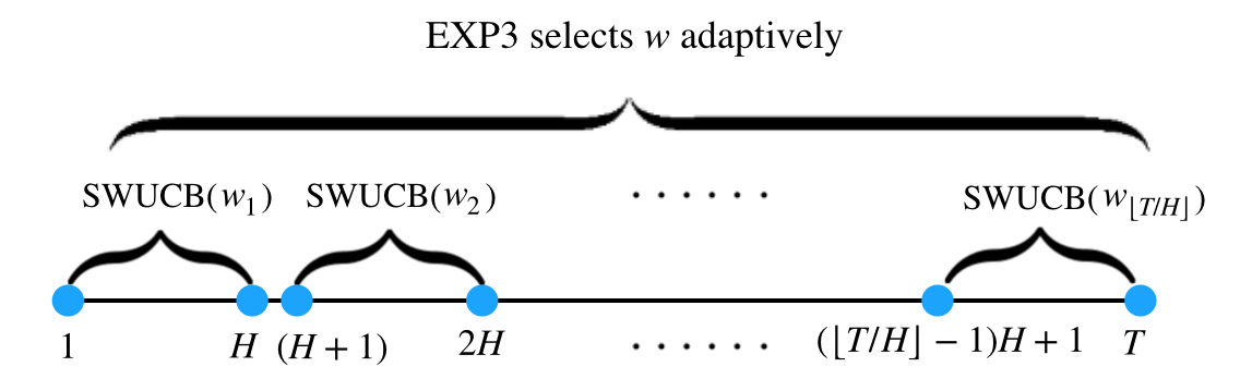
Figure 1: Structure of the BOB algorithm

Algorithm 2 BOB algorithm for drifting linear bandits

1:Input: Time horizon $T$, the SW-UCB algorithm, parameters $H,\Delta,J,Q$ (as defined in 11).

2:Initialize parameters $\gamma,\{s_{j,1}\}^{\Delta}_{j=0}$ by eq. (12).

3:for $i=1,2,\ldots,\lceil T/H\rceil$ do

4:     Define distribution $(p_{j,i})^{\Delta}_{j=0}$ by eq. (13), and set $j_{t}\leftarrow j$ with probability $p_{j,i}$.

5:     Set the window size $w_{i}\leftarrow\left\lfloor H^{j_{t}/\Delta}\right\rfloor$.

6:     Restart the SW-UCB algorithm for $H$ rounds with window size $w_{i}$.

7:     Update $s_{j_{i},i+1}$ according to eq. (14), and $s_{u,i+1}\leftarrow s_{u,i}~{}\forall u\neq j_{i}$

8:end for

To this end, we describe the details of the BOB algorithm, displayed in Algorithm 2, for the linear bandit model. Define the parameters (we justify these choices in Section 7.3)

$$H=\left\lfloor dT^{\frac{1}{2}}\right\rfloor,\Delta=\lceil\ln H\rceil,J=\left\{H^{0},\left\lfloor H^{\frac{1}{\Delta}}\right\rfloor,\ldots,H\right\},Q=2H+4R\sqrt{H\ln(T/\sqrt{H})}.$$ (11)

The BOB algorithm first divides the time horizon $T$ into $\lceil T/H\rceil$ blocks of length $H$ rounds (except for the last block, which can be less than $H$ rounds), and then initiates the parameters

$$\gamma=\min\left\{1,\sqrt{\frac{(\Delta+1)\ln(\Delta+1)}{(e-1)\lceil T/H\rceil}}\right\},s_{j,1}=1\quad\forall j=0,1,\ldots,\Delta.$$ (12)

for the EXP3 algorithm (Auer et al. 2002a). At the beginning of each block $i\in\left[\lceil T/H\rceil\right],$ the BOB algorithm first sets

$$p_{j,i}=(1-\gamma)\frac{s_{j,i}}{\sum_{u=0}^{\Delta}s_{u,i}}+\frac{\gamma}{\Delta+1}\quad\forall j=0,1,\ldots,\Delta,$$ (13)

and then sets $j_{i}=j$ with probability $p_{j,i}$ for each $j=0,1,\ldots,\Delta.$ The selected window size is then $w_{i}=\left\lfloor H^{j_{i}/\Delta}\right\rfloor.$ Afterwards, the BOB algorithm selects actions $X_{t}$ by running the SW-UCB algorithm with window size $w_{i}$ for each round $t$ in block $i,$ and the total collected reward is

$$\sum_{t=(i-1)H+1}^{i\cdot H\wedge T}Y_{t}=\sum_{t=(i-1)H+1}^{i\cdot H\wedge T}\langle X_{t},\theta_{t}\rangle+\eta_{t}.$$

Finally, the total rewards is normalized by first dividing $Q,$ and then added by $1/2$ so that it lies within $[0,1]$ with high probability. The parameter $s_{j_{i},i+1}$ is set to

$$s_{j_{i},i}\cdot\exp\left(\frac{\gamma}{(\Delta+1)p_{j_{i},i}}\left(\frac{1}{2}+\frac{\sum_{t=(i-1)H+1}^{i\cdot H\wedge T}Y_{t}}{Q}\right)\right);$$ (14)

while $s_{u,i+1}$ is the same as $s_{u,i}$ for all $u\neq j_{i}.$

7.2 Dynamic Regret Analysis

We are now ready to present the dynamic regret bound for the BOB algorithm.

Proposition 7.1

For the drifting linear bandit setting, the dynamic regret of the BOB algorithm is

$$\mathcal{R}_{T}(\texttt{BOB}\text{ algorithm})=\widetilde{O}\left(w^{{\dagger}}B_{T}+\frac{dT}{\sqrt{w^{{\dagger}}}}+Q\sqrt{\frac{|J|T}{H}}\right).$$ (15)

Proof 7.2

Proof Sketch. The complete proof is presented in Section 15 of the appendix. The dynamic regret bound (15) can be decomposed as

$$\underbrace{\widetilde{O}\left(w^{{\dagger}}B_{T}+\frac{dT}{\sqrt{w^{{\dagger}}}}\right)}_{\mathcal{R}_{T}\left(\texttt{SW-UCB}\text{ algorithm}\right)\text{ with $w^{{\dagger}}$}}+\underbrace{\widetilde{O}\left(Q\sqrt{\frac{|J|T}{H}}\right)}_{\text{Loss in learning $w^{{\dagger}}$}}.$$ (16)

The first term in (16) is due to the dynamic regret of the underlying SW-UCB algorithm under the optimally tuned window size $w^{\dagger}$. More precisely, we can view each block as a new non-stationary linear bandit instance, and the dynamic regret is due to the application of SW-UCB algorithm with window size $w^{{\dagger}}$ on each block. The second term in (16) is due to the loss by the EXP3 algorithm, which essentially treat each of the window size in $J$ as an expert, and compete with the best expert. Here, we point out due to the design of restarting, any instance of the SW-UCB algorithm cannot last for more than $H$ rounds. As a consequence, even if the EXP3 algorithm selects a window size $w_{i}>H$ for some block $i,$ the effective window size is $H.$ In other words, $w^{*}$ is not necessarily attainable, i.e., by definition, $w^{*}=\left\lfloor(dT)^{2/3}B_{T}^{-2/3}\right\rfloor$ might be larger than $H$ when $B_{T}$ is small. We thus have to denote the optimally (over $J$) tuned window size as $w^{{\dagger}}.$

Theorem 7.3

With the parameters specified in Section 7.1, the dynamic regret of the BOB algorithm for drifting linear bandit is $\mathcal{R}_{T}\left(\texttt{BOB}\text{ algorithm}\right)=\widetilde{O}\left(d^{{2}/{3}}B_{T}^{{1}/{3}}T^{{2}/{3}}+d^{{1}/{2}}T^{{3}/{4}}\right).$

The proof of Theorem 7.3 can be found in Section 16 of the appendix. In the next section, we discuss the choice of parameters in (11) and discuss its relationship

7.3 Choices of Parameters and Justifications

We first justify the choice of $Q$ in (11). Note that $Q$ is used to perform normalization, we thus prove high probability upper and lower bounds for the total rewards of each block (here, we prove a slightly more general result by allowing $\max_{t\in[T],x\in D_{t}}|\langle x,\theta_{t}\rangle|$ to be in $[-\nu,\nu]$ for some $\nu>0$).

Lemma 7.4

Suppose $\max_{t\in[T],x\in D_{t}}|\langle x,\theta_{t}\rangle|\in[-\nu,\nu]$ for some $\nu>0$ and denote $M_{i}$ as the absolute value of cumulative rewards for block $i$, then with probability at least $1-2/T,$ $M_{i}$ does not exceed $H\nu+2R\sqrt{H\ln(T/\sqrt{H})}$ for all $i,$ i.e., $\Pr\left(\forall i\in\lceil T/H\rceil\quad M_{i}\leq H\nu+2R\sqrt{H\ln\frac{T}{\sqrt{H}}}\right)\geq 1-\frac{2}{T}.$

The complete proof of Lemma 7.4 is in Section 14 of the appendix. With Lemma 7.4 and the choice of $Q=2H+4R\sqrt{H\ln(T/\sqrt{H})}$ (note that $\nu=1$ by our model assumption in Section 3), it is evident that ${\sum_{t=(i-1)H+1}^{i\cdot H\wedge T}Y_{t}}/{Q}$ in eq. (14) lies in $[-1/2,1/2]$ with probability at least $1-2/T.$ Adding this by $1/2,$ we normalize the total rewards of each block to $[0,1]$ with probability at least $1-2/T$ for all the blocks.

To determine $H,\Delta,$ and $J$, we consider the dynamic regret bound of the BOB algorithm as stated in Proposition 7.1. Eq. (15) in Proposition 7.1 exhibits a similar structure to the regret of the SW-UCB algorithm as stated in Theorem 6.1, and this immediately indicates a clear trade-off in the design of the block length $H:$

• On one hand, $H$ should be small to control the regret incurred by the EXP3 algorithm in identifying $w^{{\dagger}},$ i.e., the third term in eq. (15).

• On the others, $H$ should also be large enough to allow $w^{{\dagger}}$ to get close to $w^{*}=\lfloor(dT)^{2/3}B_{T}^{-2/3}\rfloor$ so that the sum of the first two terms in eq. (15) is minimized.

A more careful inspection also reveals the tension in the design of $J.$ Obviously, we hope that $|J|$ is small to minimize the third term in eq. (15), but we also wish $J$ to be dense enough so that it forms a cover to the set $[H].$ Otherwise, even if $H$ is large enough that $w^{{\dagger}}$ can approach $w^{*},$ approximating $w^{*}$ with any element in $J$ can cause a major loss.

These observations suggest the following choice of $J.$

$$J=\left\{H^{0},\left\lfloor H^{\frac{1}{\Delta}}\right\rfloor,\ldots,H\right\}$$ (17)

for some positive integer $\Delta,$ and since the choice of $H$ should not depend on $B_{T},$ we can set $H=\left\lfloor d^{\epsilon}T^{\alpha}\right\rfloor$ with some $\alpha\in[0,1]$ and $\epsilon>0$ to be determined. We then distinguish two cases depending on whether $w^{*}$ is smaller than $H$ or not (or alternatively, whether $B_{T}$ is larger than $d^{(2-3\epsilon)/2}T^{(2-3\alpha)/2}$ or not).

Case 1: $w^{*}\leq H$ or $B_{T}\geq d^{(2-3\epsilon)/2}T^{(2-3\alpha)/2}.$

Under this situation, $w^{{\dagger}}$ can automatically adapt to the nearly optimal window size $\text{clip}_{J}\left(w^{*}\right)$ , where $\text{clip}_{J}(x)$ finds the largest element in $J$ that does not exceed $x.$ Notice that $|J|=\Delta+1,$ the dynamic regret of the BOB algorithm then becomes

$$\mathcal{R}_{T}(\texttt{BOB}\text{ algorithm})= \widetilde{O}\left(w^{{\dagger}}B_{T}+\frac{dT}{\sqrt{w^{{\dagger}}}}+\sqrt{H|J|T}\right)$$

$$= \widetilde{O}\left(w^{*}H^{\frac{1}{\Delta}}B_{T}+\frac{dT}{\sqrt{w^{*}H^{-1/\Delta}}}+\sqrt{d^{\epsilon}T^{{\alpha+1}}\Delta}\right)$$

$$= \widetilde{O}\left(d^{\frac{2}{3}}\left(B_{T}+1\right)^{\frac{1}{3}}T^{\frac{2}{3}}H^{\frac{1}{\Delta}}+d^{\frac{\epsilon}{2}}T^{\frac{\alpha+1}{2}}\Delta^{\frac{1}{2}}\right).$$ (18)

Case 2: $w^{*}>H$ or $B_{T}<d^{(2-3\epsilon)/2}T^{(2-3\alpha)/2}.$

Under this situation, $w^{{\dagger}}$ equals to $H,$ which is the window size closest to $w^{*},$ the regret of the BOB algorithm then becomes

$$\mathcal{R}_{T}(\texttt{BOB}\text{ algorithm})= \widetilde{O}\left(w^{{\dagger}}B_{T}+\frac{dT}{\sqrt{w^{{\dagger}}}}+\sqrt{H|J|T}\right)$$

$$= \widetilde{O}\left(HB_{T}+\frac{dT}{\sqrt{H}}+\sqrt{H|J|T}\right)$$

$$= \widetilde{O}\left(d^{\epsilon}\left(B_{T}+1\right)T^{\alpha}+d^{1-\frac{\epsilon}{2}}T^{\frac{2-\alpha}{2}}++d^{\frac{\epsilon}{2}}T^{\frac{\alpha+1}{2}}\Delta^{\frac{1}{2}}\right)$$

$$= \widetilde{O}\left(d^{1-\frac{\epsilon}{2}}T^{\frac{2-\alpha}{2}}+d^{\frac{\epsilon}{2}}T^{\frac{\alpha+1}{2}}\Delta^{\frac{1}{2}}\right),$$ (19)

where we have make use of the fact that $B_{T}<d^{(2-3\epsilon)/2}T^{(2-3\alpha)/2}$ in the last step.

Now both eq. (18) and eq. (19) suggests that we should set $\Delta=\lceil\ln H\rceil,$ and eq. (19) further reveals that we should take $\alpha=1/2$ and $\epsilon=1.$ These then lead to the choice of parameters presented in eq. (11), i.e., $H=\left\lfloor dT^{\frac{1}{2}}\right\rfloor,\Delta=\lceil\ln H\rceil,J=\left\{H^{0},\left\lfloor H^{\frac{1}{\Delta}}\right\rfloor,\ldots,H\right\}.$ Here we have to emphasize that $w^{{\dagger}},\alpha,$ and $\epsilon$ are used only in the analysis, while the only parameters that we need to decide are $H,\Delta,J,$ and $Q,$ which clearly do not depend on $B_{T}.$

7.4 Further Remarks Regarding the BOB algorithm

Remark 7.5 (Removing Assumption 5)

To remove Assumption 5, one can apply a restarting strategy (Besbes et al. 2018) together with an algorithm for adversarial linear bandit, e.g., Algorithm 15 of Lattimore and Szepesvári (2018). When $B_{T}$ is known and $D_{t}$’s are fixed, by an argument similar to Theorem 2 of Besbes et al. (2018), one can show that this restarting strategy can achieve the minimax-optimal dynamic regret bound $\widetilde{O}(d^{2/3}B_{T}^{1/3}T^{2/3});$ when $B_{T}$ is unknown, we can apply the BOB algorithm to adaptively tune the restarting rate to achieve the dynamic regret bound $\widetilde{O}(d^{2/3}B_{T}^{1/3}T^{2/3}+d^{1/2}T^{3/4}).$

Remark 7.6 (Algorithm’s Optimality)

Compared with the lower bound of Theorem 4.1, the dynamic regret bound presented in Theorem 7.3 is optimal when $B_{T}\geq d^{-1/2}T^{1/4};$ while it also leaves a small $O(T^{1/12})$ gap in the worst case i.e., when $B_{T}=\Theta(1).$ This is because for the BOB algorithm, the smaller the amount of non-stationarity (as quantified in the left hand side of (1)), the harder it is for the EXP3 algorithm to detect the amount of non-stationarity, resulting in a worse dynamic regret bound. Indeed, the worst possible case for our analysis is when $B_{T}=dT^{-1/2}$ according to Theorem 4.1.

Remark 7.7 (Failure of Naive Learning of $B_{T}$)

Theorem 6.1 shows that running the SW-UCB algorithm for $T$ with window size $w^{*}=\left\lfloor(dT)^{2/3}B_{T}^{-2/3}\right\rfloor$ leads to an optimal dynamic regret. However, the choice of the window size $w^{*}$ requires the crucial knowledge of $B_{T}$, which is not available to the DM. A natural attempt would be to “learn” the unknown $B_{T}$ in order to properly tune the window size $w$. In a more restrictive setting in which the differences between consecutive $\theta_{t}$’s follow some underlying stochastic process, one possible approach is to apply a suitable machine learning technique to learn the underlying stochastic process and tune the parameter $w$ accordingly. However, under the general setting of drifting environments (1), the differences between consecutive $\theta_{t}$’s need not follow any pattern, which challenges the use of statistical machine learning algorithms for identifying the patterns on the underlying changes.

Remark 7.8 (Restarting Structure of the BOB algorithm)

The block structure and restarting the SW-UCB algorithm with a single window size for each block are essential for the correctness of the BOB algorithm. Otherwise, suppose the DM utilizes the EXP3 algorithm to select the window size $w_{t}$ for each round $t,$ and implements the SW-UCB algorithm with the selected window size without ever restarting it. Instead of eq. (15), the regret of the BOB algorithm is then decomposed as

$$\sum_{t=1}^{T}\left(\text{Reward of }\texttt{SW-UCB}\left(\left\{w^{{\dagger}}\right\}_{\tau=1}^{t}\right)\text{ in round $t$}-\text{Reward of }\texttt{SW-UCB}\left(\left\{w_{\tau}\right\}_{\tau=1}^{t}\right)\text{ in round $t$}\right)$$

$$+\sum_{t=1}^{T}\left(\text{Optimal reward in round }t-\text{Reward of }\texttt{SW-UCB}\left(\left\{w^{{\dagger}}\right\}_{\tau=1}^{t}\right)\text{ in round $t$}\right)$$ (20)

Here, with some abuse of notations, $\texttt{SW-UCB}(\{w^{{\dagger}}\}_{\tau=1}^{t})$ (respectively $(\texttt{SW-UCB}(\{w_{\tau}\}_{\tau=1}^{t})$) refers to in round $t,$ the DM runs the SW-UCB algorithm with window size $w^{{\dagger}}$ (respectively $w_{t}$) and historical data, e.g., (action, reward) pairs, generated by running the SW-UCB algorithm with window size $w^{{\dagger}}$ (respectively $w_{\tau}$) for rounds $\tau=1,\ldots,t-1.$ Same as before, the second term of eq. (7.8) can be upper bounded as a result of Theorem 6.1. It is also tempting to apply results from the EXP3 algorithm to upper bound the first term. Unfortunately, this is incorrect as it is required by the adversarial bandits protocol (Auer et al. 2002a) that the DM and its competitor should receive the same reward if they select the same action, i.e., the reward of $\texttt{SW-UCB}\left(\left\{w^{{\dagger}}\right\}_{\tau=1}^{t-1},w_{t}=w\right)$ in round $t$ and the reward of $\texttt{SW-UCB}\left(\left\{w_{\tau}\right\}_{\tau=1}^{t-1},w_{t}=w^{{\dagger}}\right)$ in round $t$ should be the same for every $w.$ Nevertheless, this is violated as running the SW-UCB algorithm with different window sizes for previous rounds can generate different (action,reward) pairs, and this results in possibly different estimated $\hat{\theta}_{t}$’s for the two SW-UCB algorithms even if both of them use the same window size in round $t.$ Hence, the selected actions and the corresponding reward by these two instances might also be different. By the careful design of blocks as well as the restarting scheme, the BOB algorithm decouples the SW-UCB algorithm for a block from previous blocks, and thus fixes the above mentioned problem, i.e., the regret of the BOB algorithm is decomposed as eq. (15).

Remark 7.9 (Applications)

The Bandit-over-Bandit framework can go beyond the problem of non-stationary bandit optimization. In a high level, it provides us a viable approach to automatically optimize the performances of data-driven sequential decision-making algorithms. Although not always optimal, it can be applied to bandit model selection (Foster et al. 2019) as well as online meta-learning (Bastani et al. 2019), in which the DM is trying to optimize the performances of her algorithms by selecting a correct model class or a set of proper parameters. Both of these are of great importance in the operations of data-driven decision-making algorithms.

8 Extensions to Other Bandit Models

In this section, we demonstrate the generality of our established results. As illustrative examples, we apply our technique to several bandit settings, including multi-armed bandits (Auer et al. 2002b), the generalized linear bandits (Filippi et al. 2010, Li et al. 2017), and the combinatorial semi-bandits (Gai et al. 2012, Kveton et al. 2015). A preview of the results is shown in Table 2. Note that for generalized linear bandits, we need to impose Assumption 5. On the other hand, for multi-armed bandits, this assumption is always valid while for combinatorial semi-bandits, this assumption is not required.

	Known $B_{T}$	Unknown $B_{T}$
$d$-armed bandit	$\widetilde{O}\left(d^{{1}/{3}}B_{T}^{{1}/{3}}T^{{2}/{3}}\right)$	$\widetilde{O}\left(d^{{1}/{3}}B_{T}^{{1}/{3}}T^{{2}/{3}}+d^{{1}/{4}}T^{{3}/{4}}\right)$
Generalized linear bandit	$\widetilde{O}\left(d^{{2}/{3}}B_{T}^{{1}/{3}}T^{{2}/{3}}\right)$	$\widetilde{O}\left(d^{{2}/{3}}B_{T}^{{1}/{3}}T^{{2}/{3}}+d^{{1}/{2}}T^{{3}/{4}}\right)$
Combinatorial semi-bandit	$\widetilde{O}\left(d^{{1}/{3}}m^{2/3}B_{T}^{{1}/{3}}T^{{2}/{3}}\right)$	$\widetilde{O}\left(d^{1/3}m^{2/3}B_{T}^{1/3}T^{2/3}+d^{1/4}m^{3/4}T^{3/4}\right)$

Table 2: Dynamic regret bounds of the SW-UCB algorithm and the BOB algorithm for different settings. Here $m$ is an upper bound for the 1-norm of all the actions in the combinatorial semi-bandit problem.

8.1 An Algorithmic Template

The SW-UCB algorithm and the BOB algorithm developed in the previous sections can be viewed as an algorithmic template that allows us to extend the results from linear bandits to other bandit settings. Given a bandit setting A, we leverage the forgetting principle (similar to Section 5), and first modify the reward estimator used in the stationary setting to a sliding-window estimator. We then incorporate it into the UCB algorithm to arrive at the corresponding SW-UCB algorithm for the drifting environments. When the variation budget is known, we could optimally tune the window size to enjoy an optimal dynamic regret bound. To achieve low dynamic regret when the variation budget is unknown, we can proceed by plugging the SW-UCB algorithm for A into the BOB algorithm, i.e., line 6 of Algorithm 2, and custom-tailor the parameters (as those listed in eq. (11)) to accommodate the need of $\texttt{A}.$

We note that the power of this algorithmic template is indeed entailed by a salient property, i.e., the dynamic regret of the SW-UCB algorithm can be decomposed as “dynamic regret of drift” + “dynamic regret of uncertainty” (or eq. (10)), that actually holds for a variety of bandit learning models in addition to linear models. In what follows, we shall derive the SW-UCB algorithm as well as the parameters required by the BOB algorithm, i.e., similar to those defined in eq. (11), for each of the above mentioned settings.

8.2 $d$-Armed Bandits

The $d$-armed bandit problem in drifting environments was first studied by (Besbes et al. 2015), who proposed Rexp3, an innovative and interesting variant of the EXP3 algorithm (Auer et al. 2003). When the underlying variation budget is known, their algorithm achieves the optimal dynamic regret bound. In this subsection, we provide an alternative derivation of the dynamic regret bound by our framework.

In the $d$-armed bandits setting, every action set $D_{t}$ is comprised of $d$ actions $e_{1},\ldots,e_{d}.$ The $i^{\text{th}}$ action $e_{i}$ has coordinate $i$ equals to 1 and all other coordinates equal to $0.$ Therefore, the reward of choosing action $X_{t}=e_{I_{t}}$ in round $t$ is $Y_{t}=\langle X_{t},\theta_{t}\rangle+\eta_{t}=\theta_{t}(I_{t})+\eta_{t},$ where $\theta_{t}(I_{t})$ is the $I_{t}^{\text{th}}$ coordinate of $\theta_{t}.$ We again assume $|\langle x,\theta_{t}\rangle|\in[-1,1]$ for all $x\in D_{t}$ and all $t\in[T].$ Different than the linear bandit setting, we follow (Besbes et al. 2015, 2018) to define the variation budget with the infinity norm, i.e., $\sum_{t=1}^{T-1}\left\|\theta_{t+1}-\theta_{t}\right\|_{\infty}\leq B_{T}.$ For a window size $w,$ we also define $N_{t-1}(i)$ as the number of times that action $i$ is chosen within rounds $(t-w),\ldots,(t-1),$ i.e., for all $i\in[d],$ $N_{t-1}(i)=\sum_{s=1\wedge(t-w)}^{t-1}\bm{1}[X_{t}=e_{i}].$ Here $\bm{1}[\cdot]$ is the indicator function. Similar to the procedure in Section 5, we set the regularization parameter $\lambda=0,$ and compute the sliding window least squares estimate $\hat{\theta}_{t}$ for $\theta_{t}$ in each round, i.e.,

$$\hat{\theta}_{t}=V_{t-1}^{*}\left(\sum^{t-1}_{s=1\vee(t-w)}X_{s}Y_{s}\right),$$ (21)

where $V_{t-1}^{*}$ is Moore-Penrose pseudo-inverse of $V_{t-1}.$ We can also derive the error bound for the latent expected reward of every action $x\in D_{t}$ in any round $t.$

Theorem 8.1

For any $t\in[T]$ and any $i\in[d],$ we have with probability at least $1-{1}/{T},$ $\left|e_{i}^{\top}(\hat{\theta}_{t}-\theta_{t})\right|\leq\sum^{t-1}_{s=1\vee(t-w)}\left\|\theta_{s}-\theta_{s+1}\right\|_{\infty}+R\sqrt{{2\ln\left({2dT^{2}}\right)}}\left\|e_{i}\right\|_{V^{*}_{t-1}}.$ holds for all $x\in D_{t}.$

The complete proof is provided in Section 17 of the appendix. We can now follow the same principle in Section 6 by choosing in each round the action $X_{t}$ with the highest UCB, i.e.,

$$X_{t}= \argmax_{x\in D_{t}}\left\{\langle x,\hat{\theta}_{t}\rangle+R\sqrt{{2\ln\left({2dT^{2}}\right)}}\left\|x\right\|_{V^{*}_{t-1}}\right\},$$ (22)

and arrive at the following regret upper bound for the SW-UCB algorithm.

Theorem 8.2

For the $d$-armed bandit setting, the dynamic regret of the SW-UCB algorithm is upper bounded as $\mathcal{R}_{T}\left(\texttt{SW-UCB}\text{ algorithm}\right)=\widetilde{O}\left(wB_{T}+\sqrt{d}T/\sqrt{w}\right).$ When $B_{T}~{}(>0)$ is known, by taking $w=\Theta\left(d^{1/3}T^{2/3}B_{T}^{-2/3}\right),$ the dynamic regret of the SW-UCB algorithm is $\mathcal{R}_{T}\left(\texttt{SW-UCB}\text{ algorithm}\right)=\widetilde{O}\left(d^{1/3}B_{T}^{1/3}T^{2/3}\right).$ When $B_{T}$ is unknown, by taking $w=\Theta\left(d^{1/3}T^{2/3}\right),$ the dynamic regret of the SW-UCB algorithm is $\mathcal{R}_{T}\left(\texttt{SW-UCB}\text{ algorithm}\right)=\widetilde{O}\left(d^{1/3}B_{T}T^{2/3}\right).$

Proof 8.3

Proof Sketch. The proof of this theorem is very similar to that of Theorem 6.1, and is thus omitted. The key difference is that $\beta$ (defined in eq. (3) for the linear bandit setting) is now set to $R\sqrt{2\ln\left(2dT^{2}\right)},$ and this saves the extra $\sqrt{d}$ factor presented in eq. (56). Hence the dynamic regret bound can be obtained accordingly.

Comparing the results obtained in Theorem 8.2 to the lower bound presented in (Besbes et al. 2015), we can easily see that the dynamic regret bound is optimal when $B_{T}$ is known. When $B_{T}$ is unknown, we can implement the BOB algorithm with the following parameters:

$$H=\left\lfloor\left(dT\right)^{\frac{1}{2}}\right\rfloor,\Delta=\lceil\ln H\rceil,J=\left\{H^{0},\left\lfloor H^{\frac{1}{\Delta}}\right\rfloor,\ldots,H\right\},Q=2H+4R\sqrt{H\ln(T/\sqrt{H})}.$$ (23)

The regret of the BOB algorithm for the MAB setting is characterized as follows.

Theorem 8.4

The dynamic regret of the BOB algorithm for the $d$-armed bandit setting is $\mathcal{R}_{T}\left(\texttt{BOB}\text{ algorithm}\right)=\widetilde{O}\left(d^{1/3}B_{T}^{1/3}T^{2/3}+d^{1/4}T^{3/4}\right).$

The proof of the theorem is very similar to Theorem 7.3’s, and it is thus omitted.

8.3 Generalized Linear Bandits

For the generalized linear bandits model, we adopt the setup in (Filippi et al. 2010, Li et al. 2017): it is essentially the same as the linear bandit setting except that the decision set is time invariant, i.e., $D_{t}=D$ for all $t\in[T],$ and the reward of choosing action $X_{t}\in D$ is $Y_{t}=\mu\left(\langle X_{t},\theta_{t}\rangle\right)+\eta_{t}.$

Let $\dot{\mu}(\cdot)$ and $\ddot{\mu}(\cdot)$ denote the first derivative and second derivative of $\mu(\cdot)$, respectively, we follow (Filippi et al. 2010) to make the following assumption. i) There exists a set of $d$ actions $a_{1},\ldots,a_{d}\in D$ such that the minimal eigenvalue of $\sum_{i=1}^{d}a_{i}a_{i}^{\top}$ is $\lambda_{0}~{}(>0).$ ii) The link function $\mu(\cdot):\mathbb{R}\to\mathbb{R}$ is strictly increasing, continuously differentiable, Lipschitz with constant $k_{\mu},$ and we define $c_{\mu}=\inf_{x\in D,\theta\in\mathbb{R}^{d}:\|\theta\|\leq S}\dot{\mu}\left(\langle x,\theta\rangle\right).$ iii) There exists $Y_{\max}>0$ such that for any $t\in[T],$ $Y_{t}\in\left[0,Y_{\max}\right].$ Similar to the procedure in Section 5, we compute the maximum quasi-likelihood estimate $\hat{\theta}_{t}$ for $\theta_{t}$ in each round $t\in[T]$ by solving the equation

$$\sum^{t-1}_{s=1\vee(t-w)}\left(Y_{s}-\mu\left(\left\langle X_{s},\hat{\theta}_{t}\right\rangle\right)\right)X_{s}=0.$$ (24)

Defining $\beta=2k_{\mu}Y_{\max}\sqrt{2d\ln(w)\ln(2dT^{2})\left(3+2\ln\left(1+2{L^{2}}/{\lambda_{0}}\right)\right)}/c_{\mu},$ we can also derive the deviation inequality type bound for the latent expected reward of every action $x\in D_{t}$ in any round $t.$ Here, as pointed out in Faury et al. (2021), we need to assume that $\|\hat{\theta}_{t}\|\leq S$ holds for every $t\in[T]$. Otherwise, we need to perform a projection step similar to Filippi et al. (2010), Faury et al. (2021).

Theorem 8.5

For any $t\in[T],$ we have with probability at least $1-1/T,$ $\left|\mu\left(x^{\top}\hat{\theta}_{t}\right)-\mu\left(x^{\top}\theta_{t}\right)\right|\leq\frac{k^{2}_{\mu}L}{c_{\mu}}\sum^{t-1}_{s=1\vee(t-w)}\left\|\theta_{s}-\theta_{s+1}\right\|_{2}+\beta\left\|x\right\|_{V^{-1}_{t-1}}$ holds for all $x\in D_{t}.$

Proof 8.6

Proof Sketch. The proof is a consequence of Proposition 1 of (Filippi et al. 2010) and Theorem 5.2. Please refer to Section 18 of the appendix for the complete proof.

We can now follow the same principle in Section 6 to design the SW-UCB algorithm. Note that in order for $V_{t-1}$ to be invertible for all $t,$ our algorithm should select the actions $a_{1},\ldots,a_{d}$ every $w$ rounds for some window size $w.$ For each of the remaining round $t,$ it chooses the action $X_{t}$ with the highest UCB, i.e.,

$$X_{t}= \argmax_{x\in D_{t}}\left\{\langle x,\hat{\theta}_{t}\rangle+\beta\left\|x\right\|_{V^{*}_{t-1}}\right\},$$ (25)

and arrive at the following regret upper bound.

Theorem 8.7

For the drifting generalized linear bandit setting, the dynamic regret of the SW-UCB algorithm is upper bounded as $\mathcal{R}_{T}\left(\texttt{SW-UCB}\text{ algorithm}\right)=\widetilde{O}\left(wB_{T}+dT/\sqrt{w}\right).$ When $B_{T}~{}(>0)$ is known, by taking $w=\Theta\left((dT)^{2/3}B_{T}^{-2/3}\right),$ the dynamic regret of the SW-UCB algorithm is $\mathcal{R}_{T}\left(\texttt{SW-UCB}\text{ algorithm}\right)=\widetilde{O}\left(d^{2/3}B_{T}^{1/3}T^{2/3}\right).$ When $B_{T}$ is unknown, by taking $w=\Theta\left((dT)^{2/3}\right),$ the dynamic regret of the SW-UCB algorithm is $\mathcal{R}_{T}\left(\texttt{SW-UCB}\text{ algorithm}\right)=\widetilde{O}\left(d^{2/3}B_{T}T^{2/3}\right).$

Proof 8.8

Proof Sketch. The proof of this theorem is similar to that of Theorem 6.1, and is thus omitted. The only difference is that we need to include the regret contributed by selecting actions $a_{1},\ldots,a_{d}$ every $w$ rounds. But these sums to $\widetilde{O}\left(dT/w\right),$ which is dominated by the term $\widetilde{O}\left(dT/\sqrt{w}\right).$ Hence the dynamic regret bounds can be obtained similarly as the linear bandit setting.

We can now implement the BOB algorithm with the same set of parameters as eq. (11), except that $Q$ is set to $H\cdot Y_{\max},$ i.e.,

$$H=\left\lfloor\left(dT\right)^{\frac{1}{2}}\right\rfloor,\Delta=\lceil\ln H\rceil,J=\left\{H^{0},\left\lfloor H^{\frac{1}{\Delta}}\right\rfloor,\ldots,H\right\},Q=2H\cdot Y_{\max}.$$ (26)

This is because the total rewards of each block is deterministically bounded by $[-H\cdot Y_{\max},H\cdot Y_{\max}].$ The dynamic regret bound when $B_{T}$ is unknown thus follows.

Theorem 8.9

The dynamic regret bound of the BOB algorithm for the drifting generalized linear bandit setting is $\mathcal{R}_{T}\left(\texttt{BOB}\text{ algorithm}\right)=\widetilde{O}\left(d^{2/3}B_{T}^{1/3}T^{2/3}+d^{1/2}T^{3/4}\right).$

The proof of the theorem is similar to Theorem 7.3’s, and it is thus omitted.

8.4 Combinatorial Semi-Bandits

Finally, we consider the drifting combinatorial semi-bandit problem. For ease of presentation, we use $X(i)$ to denote the $i^{\text{th}}$ coordinate of a vector $X.$ Following the setup in Kveton et al. (Kveton et al. 2015), an instance of combinatorial semi-bandit is represented by the tuple $(E,\mathcal{E},\{P_{t}\}^{T}_{t=1}),$ where the ground set $E$ consist of $d$ items, and ${\cal E}$ is a family of indicator vectors of subsets of $E$. Each $P_{t}$ is a latent distribution on the reward vector $W_{t}=(W_{t}(1),\ldots W_{t}(d))$ on each and every item $i\in E$ in round $t\in[T].$ The DM only knows that $W_{t}(i)$ belongs to $[0,1]$ for each $i\in[d]$ and $t\in[T]$, but she does not know $\theta_{t}(i)=\mathbb{E}[W_{t}(i)]$ for any $i\in[d]$ and $t\in[T].$ We can thus know from Lemma 1.8 of Rigollet and Hütter (Rigollet and Hütter 2018) that $W_{t}(i)-\theta_{t}(i)$ is $R=1/2$ sub-Gaussian for all $t\in[T]$ and $i\in[d]$. The sequence $\{P_{t}\}^{T}_{t=1}$ are generated by an oblivious adversary before the online process begins.

In each round $t,$ a reward vector $W_{t}$ is sampled according to the latent distribution $P_{t}$. Then, the DM pulls an action $X_{t}\in{\cal E}_{t}$, and earns a reward $Y_{t}=\langle X_{t},W_{t}\rangle=\sum_{i\in E}X_{t}(i)W_{t}(i)$ that corresponds to the items indicated by $X_{t}$. Under the semi-bandit feedback model, the DM observes the realized rewards $\{W_{t}(i):X_{t}(i)=1\}$ for the indicated items, but she does not observe $W_{t}(i)$ for $X_{t}(i)=0$. The DM desires to minimize the dynamic regret $\mathbb{E}\left[\sum^{T}_{t=1}\max_{x_{t}^{*}\in\mathcal{E}}\langle x_{t}^{*}-X_{t},\theta_{t}\rangle\right].$ Similar to the $d$-armed bandit setting, we define the variation budget $B_{T}$ with the infinity norm: $\sum^{T-1}_{t=1}\|\theta_{t+1}-\theta_{t}\|_{\infty}\leq B_{T}.$ For the subsequent discussion, we denote $m=\max_{X\in{\cal E}}\sum_{i\in E}X(i)$ as the maximum arm size of the underlying instance.

We first show a lower bound for this setting.

Theorem 8.10

Let $(d,m,T,B_{T})$ be a tuple that satisfies inequalities $d\geq 2m\geq 2$, $T\geq 1$, $m/d\leq B_{T}\leq Tm/d$. For any non-anticipatory policy, there exists a drifting combinatorial bandit instance $(E,\mathcal{E},\{P_{t}\}^{T}_{t=1}),$ with $d$ items, maximum arm size $m$, and variation budget $B_{T}$ such that the dynamic regret in $T$ rounds is $\Omega(d^{1/3}m^{2/3}B_{T}^{1/3}T^{2/3}).$

The complete proof is presented in Section 19 of the appendix. For a window size $w,$ we define $N_{t-1}(i)$ as the number of times that coordinate $i$ of the chosen action is set to $1$ within rounds $(t-w),\ldots,(t-1),$ i.e., for all $i\in[d],$ $N_{t-1}(i)=\sum^{t-1}_{s=1\vee(t-w)}\mathbf{1}[X_{s}(i)=1].$ Here $\bm{1}[\cdot]$ is the indicator function. In each round $t$, the DM also maintains the sliding-window estimates for each coordinate $i\in[d]$ of $\theta_{t}$:

$$\hat{\theta}_{t}(i)=\frac{\sum^{t-1}_{s=1\vee(t-w)}W_{s}(i)\cdot\mathbf{1}[X_{s}(i)=1]}{\max\{N_{i,t-1},1\}}.$$

Thanks to the semi-bandit feedback, the outcome $W_{s}(i)$ is observed when $X_{s}(i)=1$, so $\hat{\theta}_{t,i}$ can be constructed from the observations in the previous $w$ rounds. We can thus reuse the Theorem 8.1 derived for the $d$-armed bandit case:

Theorem 8.11

For all $t\in[T]$ and all $i\in[d],$ we have with probability at least $1-{1}/{T},$ $\left|\hat{\theta}_{t}(i)-\theta_{t}(i)\right|\leq\sum^{t-1}_{s=1\vee(t-w)}\left\|\theta_{s}-\theta_{s+1}\right\|_{\infty}+4R\sqrt{\frac{\ln(2dT^{2})}{N_{t-1}(i)+1}},$ holds for all $x\in D_{t}.$

The complete proof is presented in Section 20. Following the rationale of UCB algorithm for stochastic combinatorial semi-bandit (Kveton et al. 2015) as well as that of Section 6, we consider the SW-UCB algorithm which selects a combinatorial action $X_{t}$ with highest UCB in each round $t$, i.e.,

$$\max_{X\in{\cal E}_{t}}\left\{\sum_{i\in E}X(i)\cdot\left[\hat{\theta}_{t,i}+4R\sqrt{\frac{\ln(2dT^{2})}{N_{t-1}(i)+1}}\right]\right\}.$$

Denoting $m:=\max_{t\in[T],X\in\mathcal{E}_{t}}\|X\|_{1}$, we can now arrive at the following regret upper bound.

Theorem 8.12

For any window size $w\geq d/m,$ the dynamic regret of the SW-UCB algorithm for the drifting combinatorial semi-bandit setting is upper bounded as $\mathcal{R}_{T}\left(\texttt{SW-UCB}\text{ algorithm}\right)=\widetilde{O}\left(wmB_{T}+{\sqrt{dm}T}/{\sqrt{w}}\right).$ When $B_{T}<mT/d,$ is known, by taking $w=\Theta\left(d^{1/3}m^{-1/3}T^{2/3}B_{T}^{-2/3}\right),$ the dynamic regret of the SW-UCB algorithm is $\mathcal{R}_{T}\left(\texttt{SW-UCB}\text{ algorithm}\right)=\widetilde{O}\left(d^{1/3}m^{2/3}B_{T}^{1/3}T^{2/3}\right).$ When $B_{T}$ is unknown, by taking $w=\Theta\left(d^{1/3}m^{-1/3}T^{2/3}\right),$ the dynamic regret of the SW-UCB algorithm is $\mathcal{R}_{T}\left(\texttt{SW-UCB}\text{ algorithm}\right)=\widetilde{O}\left(d^{1/3}m^{2/3}B_{T}T^{2/3}\right).$

The complete proof is presented in Section 21 of the appendix. When $B_{T}$ is unknown, we can implement the BOB algorithm with the following parameters:

$$H=\left\lfloor\left(dT\right)^{\frac{1}{2}}m^{-\frac{1}{2}}\right\rfloor,\Delta=\lceil\ln H\rceil,J=\left\{H^{0},\left\lfloor H^{\frac{1}{\Delta}}\right\rfloor,\ldots,H\right\},Q=2H\cdot m$$ (27)

This is because the total rewards of each block is deterministically bounded by $[-H\cdot m,H\cdot m].$ The dynamic regret bound of the BOB algorithm for the combinatorial semi-bandit setting is characterized as follows.

Theorem 8.13

The dynamic regret of the BOB algorithm for the drifting combinatorial semi-bandit setting is $\mathcal{R}_{T}\left(\texttt{BOB}\text{ algorithm}\right)=\widetilde{O}\left(d^{1/3}m^{2/3}B_{T}^{1/3}T^{2/3}+d^{1/4}m^{3/4}T^{3/4}\right).$

The complete proof is presented in Section 22.

9 Numerical Experiments

As a complement to our theoretical results, we conduct numerical experiments on synthetic datasets and the CPRM-12-001: On-Line Auto Lending dataset provided by the Center for Pricing and Revenue Management at Columbia University to compare the dynamic regret performances of the SW-UCB algorithm and the BOB algorithm with several existing non-stationary bandit algorithms.

9.1 Experiments on Synthetic Dataset

For synthetic dataset, in Section 9.1.1, we first evaluate the growth of dynamic regret when $T$ increases. We follow the setup of (Besbes et al. 2018) for fair comparisons. Then, in Section 9.1.2, we fix $T=10^{5}$, and evaluate the behavior of the algorithms across rounds.

9.1.1 The Trend of Dynamic Regret with Varying $T$

We consider a 2-armed bandit setting, and we vary $T$ from $3\times 10^{4}$ to $2.4\times 10^{5}$ with a step size of $3\times 10^{4}.$ We set $\theta_{t}$ to be the following sinusoidal process, i.e., $\forall t\in[T],$ $\theta_{t}=\begin{pmatrix}0.5+0.3\sin\left({5B_{T}\pi t}/{T}\right),0.5+0.3\sin\left(\pi+{5B_{T}\pi t}/{T}\right)\end{pmatrix}^{\top}.$ The total variation of the $\theta_{t}$’s across the whole time horizon is upper bounded by $\sqrt{2}B_{T}.$ We also use i.i.d. normal distribution with $R=0.1$ for the noise terms.

Known Constant Variation Budget.

We start from the known constant variation budget case, i.e., $B_{T}=1,$ to measure the regret growth of the two optimal algorithms, i.e., the optimally tuned (i.e., knowing $B_{T}$) SW-UCB algorithm and the modified EXP3.S algorithm (Besbes et al. 2015), with respect to the total number of rounds. The log-log plot is shown in Fig. 2(a). From the plot, we can see that the regret of SW-UCB algorithm is only about $20\%$ of the regret of EXP3.S algorithm.

Unknown Time-Dependent Variation Budget.

We then turn to the more realistic time-dependent variation budget case, i.e., $B_{T}=T^{1/3}.$ As the modified EXP3.S algorithm does not apply to this setting, we compare the performances of the obliviously tuned (i.e., not knowing $B_{T}$) SW-UCB algorithm and the BOB algorithm. The log-log plot is shown in Fig. 2(b). From the results, we verify that the slope of the regret growth of both algorithms roughly match the established results, and the regret of BOB algorithm’s is much smaller than that of the SW-UCB algorithm’s.

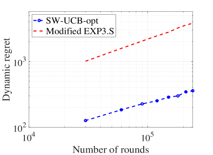
(a) Log-log plot for known $B_{T}=O(1).$

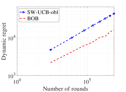
(b) Log-log plot for unknown $B_{T}=O(T^{1/3}).$

Figure 2: Results for gradually change environment with 2 arms

9.1.2 A Further Study on the Algorithms’ Behavior

We provide additional numerical evaluation, by considering piecewise linear instances, where the reward vector $\theta_{t}\in\mathbb{R}^{d}$ is a randomly generated piecewise linear function of $t$. To generate such an instance, we first set $T=10^{5}$, and then we randomly sample 30 time points in $\tau_{1},\tau_{2},\ldots,\tau_{30}\in\{2,\ldots,T-1\}$ without replacement. We further denote $\tau_{0}=1,\tau_{31}=T$. After that, we randomly sample 32 random unit length vectors $v_{0},\ldots,v_{31}\in\mathbb{R}^{d}$. Finally, for each $t\in[T]$, we define $\theta_{t}$ as the linear interpolation between $v_{s},v_{s+1}$, where $\tau_{s}\leq t\tau_{s+1}$. More precisely, we have $\theta_{t}=((\tau_{s+1}-t)v_{s}+(t-\tau_{s})v_{s+1})/(\tau_{s+1}-\tau_{s})$. Note that the random reward in each period can be negative.

In what follows, we first evaluate the performance of the algorithms by (Besbes et al. 2018) as well as our algorithms in a 2-armed bandit piece-wise linear instance. Then, we evaluate the performance of our algorithms in a linear bandit piece-wise linear instance, where $d=5$, and each $D_{t}$ is a random subset of 40 unit length vectors in $\mathbb{R}^{d}$. We do not evaluate the algorithms by (Besbes et al. 2018) in the second instance, since the algorithms by (Besbes et al. 2018) are only designed for the non-stationary $K$-armed bandit setting. For each instance, each algorithm is evaluated 50 times.

Two armed bandits.

We first evaluate the performance of the modified EXP.3S in (Besbes et al. 2018) as well as the performance of the SW-UCB algorithm, BOB algorithmin a randomly generated 2-armed bandit instance. Fig 3(a) illustrates the average cumulative reward earned by each algorithm in the 50 trials, and Fig 3(b) depicts the average dynamic regret incurred by each algorithm in the 50 trials. In Figs 3(a), 3(b), shorthand SW-UCB-opt is the SW-UCB algorithm, where $B_{T}$ is known and $w=w^{\text{opt}}$ is set to further optimized the log factors of the dynamic regret bound (see Appendix 23 for the expression of $w^{\text{opt}}$). Shorthand EXP3.S stands for the modified EXP3.S algorithm by (Besbes et al. 2018), where $B_{T}$ is known and the window size is set to optimized the dynamic regret bound. Shorthand BOB stands for the BOB algorithm. Shorthand SW-UCB-obl is the SW-UCB algorithm, where $B_{T}$ is not known, and $w=w^{\text{obl}}$ is obliviously set (see Appendix 23 for the expression of $w^{\text{obl}}$). Finally, shorthand UCB stands for the UCB algorithm by (Abbasi-Yadkori et al. 2011), which is applicable to the stationary $K$-armed bandit problem. Note that $B_{T}$ is known to SW-UCB-opt, EXP3.S, but not to BOB, SW-UCB-obl, UCB.

Overall, we observe that SW-UCB-opt is the better performing algorithm when $B_{T}$ is known, and BOB is the best performing when $B_{T}$ is not known. It is evident from Fig 3(a) that SW-UCB-opt, EXP3.S and BOB are able to adapt to the change in the reward vector $\theta_{t}$ across time $t$. We remark that BOB, which does not know $B_{T}$, achieves a comparable amount of cumulative reward to EXP3.S, which does know $B_{T}$, across time. It is also interesting to note that UCB, which is designed for the stationary setting, fails to converge (or even to achieve a non-negative total reward) in the long run, signifying the need of an adaptive UCB algorithm in a non-stationary setting.

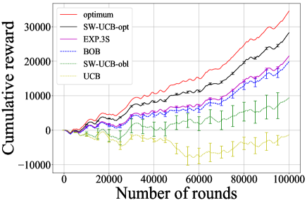
(a) Cumulative reward

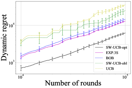
(b) Dynamic regret

Figure 3: Results for piecewise linear environment with 2 arms

Linear bandits.

Next, we move to the linear bandit case, and we consider the performance of SW-UCB-opt, SW-UCB-obl, BOB and UCB, as illustrated in Figs 4(a), 4(b). While the performance of the algorithms ranks similarly to the previous 2-armed bandit case, we witness that UCB, which is designed for the stationary setting, has a much better performance in the current case than the 2-armed case. We surmise that the relatively larger size of the action space $D_{t}$ here allows UCB to choose an action that performs well even when the reward vector is changing.

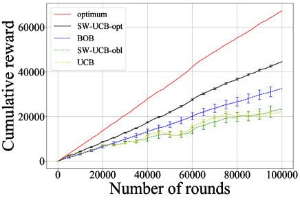
(a) Cumulative reward

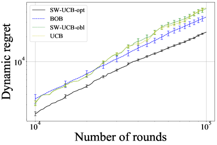
(b) Dynamic Regret

Figure 4: Results for piecewise linear environment with linear action set.

9.2 Experiments on Online Auto-Lending Dataset

We now conduct experiments on the on-line auto lending dataset, which was first studied by (Phillips et al. 2015), and subsequently used to evaluate dynamic pricing algorithms by (Ban and Keskin 2018). The dataset records all auto loan applications received by a major online lender in the United States from July 2002 through November 2004. Note that this was the time amid the severe acute respiratory syndrome (SARS) epidemic period (World Health Organization (2003) WHO), and one could thus expect high volatility in demand similar to the COVID-19 pandemic period. Each datum consists of the borrower’s feature (e.g., date of an application, the term and amount of loan requested, and some personal information), the lender’s decision (e.g., the monthly payment for the borrower), and whether or not this offer is accepted by the borrower. Please refer to Columbia University Center for Pricing and Revenue Management (Columbia 2015) for a detailed description of the dataset.

Similar to Ban and Keskin (2018), we use the first $T=5\times 10^{4}$ arrivals that span 276 days for this experiment. We adopt the commonly used (Li et al. 2010, Besbes and Zeevi 2015) linear regression model to interpolate the response of each customer: for the $t^{\text{th}}$ customer with feature $x_{t},$ if price $p_{t}$ is offered, she accepts the offer with “probability” $\langle\theta_{t},[x_{t};p_{t}x_{t}]\rangle.$ Although the customers’ responses are binary, i.e., whether or not she accepts the loan, (Besbes and Zeevi 2015) theoretically justified that the revenue loss caused by using this misspecified model is negligible. For the changing environment, we consider a piecewise stationary environment. In particular, we assume that the $\theta_{t}$’s remain stationary in a single day period, but can change across days. We also use the feature selection results in (Ban and Keskin 2018) to pick the FICO score, the term of contract, the loan amount approved, prime rate, the type of car, and the competitor’s rate as the feature vector for each customer.

Firstly, we recover the latent parameters $\theta_{t}$’s from the dataset with linear regression method. Since the lender’s decisions, i.e., the price for each customer, is not presented in the dataset, we impute the price of a loan as the net present value of future payments (a function of the monthly payment, customer rate, and term approved, please refer to (Columbia 2015, Ban and Keskin 2018) for more details). The resulted $B_{T}$ is $1.9\times 10^{2}~{}\left(\approx T^{0.48}\right),$ which means we are in the moderately non-stationary environment. Since the maximum of the imputed prices is $\approx 400,$ the range of price in our experiment is thus set to $[0,500]$ with a step size of 10.

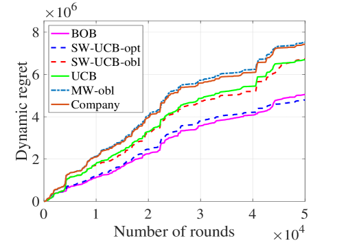
Figure 5: Results for the on-line auto lending dataset.

We then run the experiment with the recovered parameters, and measure the dynamic regrets of the SW-UCB algorithm (known $B_{T}$ and unknown $B_{T}$), the BOB algorithm, the UCB algorithm, the Moving Window (MW) algorithm (Keskin and Zeevi 2016) without knowing $B_{T}$, as well as the company’s original decisions. Here, we note that the MW algorithm does not permit customer features, and hence its dynamic regret should scale linearly in $T$. The results are shown in Fig. 5. The plot shows that the SW-UCB algorithm with known $B_{T}$ (SW-UCB-opt) and the BOB algorithm have the lowest dynamic regrets. Besides, the dynamic regret of the parameter-free BOB algorithm is $\geq 24\%$ less than those of the obliviously tuned SW-UCB algorithm (SW-UCB-obl) and the UCB algorithm. It also saves $\geq 32\%$ dynamic regret when compared to the MW algorithm and the company’s original decisions. The results clearly indicate that the SW-UCB algorithm and the BOB algorithm can deal with the drift while the UCB algorithm fails to keep track of the dynamic environment. More importantly, the results validate our theoretical findings regarding the parameter-free adaptation of the BOB algorithm.

10 Conclusion

In this paper, we develop general data-driven decision-making algorithms with state-of-the-art dynamic regret bounds in various non-stationary bandit settings. We characterize a minimax dynamic regret lower bound, and present a tuned Sliding Window Upper-Confidence-Bound algorithm with matching dynamic regret bounds. We further propose the parameter-free Bandit-over-Bandit framework that automatically adapts to the unknown non-stationarity. Finally, we conduct extensive numerical experiments on both synthetic and real-world datasets to validate our theoretical results. The authors thank the department editor J.George Shanthikumar, the anonymous associate editor, and three anonymous referees whose comments improved the manuscript. The previous version of the current paper contains an error in the proof of Theorem 5.2. Fixing this requires Assumption 5, which was first introduced by Faury et al. (2021). The authors would like to express sincere gratitude to Omar Besbes, Xi Chen, Dylan Foster, Yonatan Gur, Yujia Jin, Akshay Krishnamurthy, Haipeng Luo, Sasha Rakhlin, Vincent Tan, Kuang Xu, Assaf Zeevi, as well as various seminar attendees for helpful discussions and comments. The authors also gratefully acknowledge Columbia University Center for Pricing and Revenue Management for providing us the dataset on auto loans. This research is supported by the Ministry of Education, Singapore, under its 2019 Academic Research Fund Tier 3 grant call (Award ref: MOE-2019-T3-1-010). The research is also supported by the MIT Data Science Lab, a lab focused on the development of analytic techniques and tools for improving decision making in environments that involve uncertainty and require statistical learning.

Proofs

11 Proof of Theorem 4.1

First, let’s review the lower bound of the linear bandit setting, which is related to ours except that the $\theta_{t}$’s do not vary across rounds, and are equal to the same (unknown) $\theta,$ i.e., $\forall t\in[T]~{}\theta_{t}=\theta.$

Lemma 11.1 ((Lattimore and Szepesvári 2018))

For any $T_{0}\geq\sqrt{d}/2$ and let $D=\left\{x\in\mathbb{R}^{d}:\|x\|\leq 1\right\},$ then there exists a $\theta\in\left\{\pm\sqrt{d/4T_{0}}\right\}^{d},$ such that the worst case regret of any algorithm for linear bandits with unknown parameter $\theta$ is $\Omega(d\sqrt{T_{0}}).$

Going back to the non-stationary environment, suppose nature divides the whole time horizon into $\lceil T/H\rceil$ blocks of equal length $H$ rounds (the last block can possibly have less than $H$ rounds), and each block is a decoupled linear bandit instance so that the knowledge of previous blocks cannot help the decision within the current block. Following Lemma 11.1, we restrict the sequence of $\theta_{t}$’s are drawn from the set $\left\{\pm\sqrt{d/4H}\right\}^{d}.$ Moreover, $\theta_{t}$’s remain fixed within a block, and can vary across different blocks, i.e.,

$$\forall i\in\left[\left\lceil\frac{T}{H}\right\rceil\right]\forall t_{1},t_{2}\in[(i-1)H+1,i\cdot H\wedge T]\quad\theta_{t_{1}}=\theta_{t_{2}}.$$ (28)

We argue that even if the DM knows this additional information, it still incur a regret $\Omega(d^{2/3}B_{T}^{1/3}T^{2/3}).$ Note that different blocks are completely decoupled, and information is thus not passed across blocks. Therefore, the regret of each block is $\Omega\left(d\sqrt{H}\right),$ and the total regret is at least

$$\left(\left\lceil\frac{T}{H}\right\rceil-1\right)\Omega\left(d\sqrt{H}\right)=\Omega\left(dTH^{-\frac{1}{2}}\right).$$ (29)

Intuitively, if $H,$ the number of length of each block, is smaller, the worst case regret lower bound becomes larger. But too small a block length can result in a violation of the variation budget. So we work on the total variation of $\theta_{t}$’s to see how small can $H$ be. The total variation of the $\theta_{t}$’s can be seen as the total variation across consecutive blocks as $\theta_{t}$ remains unchanged within a single block. Observe that for any pair of $\theta,\theta^{\prime}\in\left\{\pm\sqrt{d/4H}\right\}^{d},$ the $\ell_{2}$ difference between $\theta$ and $\theta^{\prime}$ is upper bounded as

$$\sqrt{\sum_{i=1}^{d}\frac{4d}{4H}}=\frac{d}{\sqrt{H}}$$ (30)

and there are at most $\lfloor T/H\rfloor$ changes across the whole time horizon, the total variation is at most

$$B=\frac{T}{H}\cdot\frac{d}{\sqrt{H}}={dTH^{-\frac{3}{2}}}.$$ (31)

By definition, we require that $B\leq B_{T},$ and this indicates that

$$H\geq(dT)^{\frac{2}{3}}B_{T}^{-\frac{2}{3}}.$$ (32)

Taking $H=\left\lceil{(dT)^{\frac{2}{3}}B_{T}^{-\frac{2}{3}}}\right\rceil,$ the worst case regret is

$$\Omega\left(dT\left((dT)^{\frac{2}{3}}B_{T}^{-\frac{2}{3}}\right)^{-\frac{1}{2}}\right)=\Omega\left(d^{\frac{2}{3}}B_{T}^{\frac{1}{3}}T^{\frac{2}{3}}\right).$$ (33)

Note that in order for $H\leq T,$ we require $B_{T}\geq dT^{-1/2}.$ Also, to make $|\langle x,\theta_{t}\rangle|\leq 1$ for all $t\in[T]$ and $x\in D_{t},$ we need $\|\theta_{t}\|\leq 1,$ which means $\sqrt{d^{2}/4H}\leq 1$ or $B_{T}\leq 8d^{-2}T.$

12 Proof of Theorem 5.2

The difference $\hat{\theta}_{t}-\theta_{t}$ has the following expression:

$$V_{t-1}^{-1}\left(\sum_{s=1\vee(t-w)}^{t-1}X_{s}X_{s}^{\top}\theta_{s}+\sum_{s=1\vee(t-w)}^{t-1}\eta_{s}X_{s}\right)-\theta_{t}$$

$$= V_{t-1}^{-1}\sum_{s=1\vee(t-w)}^{t-1}X_{s}X_{s}^{\top}\left(\theta_{s}-\theta_{t}\right)+V_{t-1}^{-1}\left(\sum_{s=1\vee(t-w)}^{t-1}\eta_{s}X_{s}-\lambda\theta_{t}\right),$$ (34)

The first term on the right hand side of eq. (34) is the estimation inaccuracy due to the non-stationarity; while the second term is the estimation error due to random noise. We now upper bound the two terms separately. We upper bound the first term under the Euclidean norm.

Lemma 12.1

For any $t\in[T],$ we have

$$\left\|V_{t-1}^{-1}\sum_{s=1\vee(t-w)}^{t-1}X_{s}X_{s}^{\top}\left(\theta_{s}-\theta_{t}\right)\right\|_{2}\leq\sum^{t-1}_{s=1\vee(t-w)}\left\|\theta_{s}-\theta_{s+1}\right\|_{2}.$$

Proof 12.2

Poof. In the proof, we denote $B(1)$ as the unit Euclidean ball, and $\lambda_{\text{max}}(M)$ as the maximum eigenvalue of a square matrix $M$. In addition, recall the definition that $V_{t-1}=\lambda I+\sum^{t-1}_{s=1\vee(t-w)}X_{s}X_{s}^{\top}$ We prove the Lemma as follows:

$$\left\|V_{t-1}^{-1}\sum_{s=1\vee(t-w)}^{t-1}X_{s}X_{s}^{\top}\left(\theta_{s}-\theta_{t}\right)\right\|_{2}$$

$$= \left\|V_{t-1}^{-1}\sum_{s=1\vee(t-w)}^{t-1}X_{s}X_{s}^{\top}\left[\sum^{t-1}_{p=s}\left(\theta_{p}-\theta_{p+1}\right)\right]\right\|_{2}$$

$$= \left\|V_{t-1}^{-1}\sum^{t-1}_{p=1\vee(t-w)}\sum_{s=1\vee(t-w)}^{p}X_{s}X_{s}^{\top}\left(\theta_{p}-\theta_{p+1}\right)\right\|_{2}$$ (35)

$$\leq \sum^{t-1}_{p=1\vee(t-w)}\left\|V_{t-1}^{-1}\left(\sum_{s=1\vee(t-w)}^{p}X_{s}X_{s}^{\top}\right)\left(\theta_{p}-\theta_{p+1}\right)\right\|_{2}$$ (36)

$$\leq \sum^{t-1}_{p=1\vee(t-w)}\sqrt{\lambda_{\text{max}}\left(\left(\sum_{s=1\vee(t-w)}^{p}X_{s}X_{s}^{\top}\right)V_{t-1}^{-2}\left(\sum_{s=1\vee(t-w)}^{p}X_{s}X_{s}^{\top}\right)\right)}\left\|\theta_{p}-\theta_{p+1}\right\|_{2}$$ (37)

$$\leq \sum^{t-1}_{p=1\vee(t-w)}\left\|\theta_{p}-\theta_{p+1}\right\|_{2}.$$ (38)

Equality (35) is by the observation that both sides of the equation is summing over the terms $X_{s}X^{\top}_{s}(\theta_{p}-\theta_{p+1})$ with indexes $(s,p)$ ranging over $\{(s,p):1\vee(t-w)\leq s\leq p\leq t-1\}$. Inequality (36) is by the triangle inequality.

Inequality (37) is by the fact that, for any matrix $M\in\mathbb{R}^{d\times d}$ with $\lambda_{\text{max}}(M)\geq 0$ and any vector $y\in\mathbb{R}^{d}$, we have $\left\|My\right\|_{2}\leq\sqrt{\lambda_{\text{max}}(M^{2})}\left\|y\right\|_{2}$. Applying the above claim with $M=V_{t-1}^{-1}\left(\sum_{s=1\vee(t-w)}^{p}X_{s}X_{s}^{\top}\right)$ and $y=\theta_{p}-\theta_{p+1}$ demonstrates inequality (37).

Finally, for inequality (38), we denote the corresponding basis for each $X_{s}$ as $\psi_{i(s)},$ i.e., $X_{s}=z_{s}\psi_{i(s)}=z_{s}\Psi e_{i(s)},$ where $e_{i}$ is the $i^{\text{th}}$ standard orthonormal basis. Let $A_{1}=\sum_{s=1\vee(t-w)}^{t-1}e_{i(s)}e_{i(s)}^{\top}+\lambda I$ and $A_{2}=\sum_{s=1\vee(t-w)}^{p}e_{i(s)}e_{i(s)}^{\top},$ it is evident that $V_{t-1}=\Psi A_{1}\Psi^{\top}$ and $\sum_{s=1\vee(t-w)}^{p}X_{s}X_{s}^{\top}=\Psi A_{2}\Psi^{\top}.$ Therefore, we have

$$\lambda_{\text{max}} \left(\left(\sum_{s=1\vee(t-w)}^{p}X_{s}X_{s}^{\top}\right)V_{t-1}^{-2}\left(\sum_{s=1\vee(t-w)}^{p}X_{s}X_{s}^{\top}\right)\right)=\lambda_{\text{max}}\left(\Psi A_{2}\Psi^{\top}(\Psi A_{1}\Psi^{\top})^{-2}\Psi A_{2}\Psi^{\top}\right)$$

$$=\lambda_{\text{max}}\left(\Psi A_{2}A^{-2}_{1}A_{2}\Psi^{\top}\right)=\lambda_{\text{max}}\left(A_{2}A^{-2}_{1}A_{2}\right)\leq 1,$$ (39)

where we have used the fact that both $A_{1}$ and $A_{2}$ are diagonal matrix in the last step. Altogether, the Lemma is proved.

Applying Theorem 2 of (Abbasi-Yadkori et al. 2011), we have the following upper bound for the second term in eq. (2).

Lemma 12.3 ((Abbasi-Yadkori et al. 2011))

For any $t\in[T]$ and any $\delta\in[0,1],$ we have

$$\left\|\sum_{s=1\vee(t-w)}^{t-1}\eta_{s}X_{s}-\lambda\theta_{t}\right\|_{V_{t-1}^{-1}}\leq R\sqrt{d\ln\left(\frac{1+wL^{2}/\lambda}{\delta}\right)}+\sqrt{\lambda}S$$

holds with probability at least $1-\delta.$

Combining the above two lemmas: fixed any $\delta\in[0,1],$ we have that for any $t\in[T]$ and any $x\in D_{t},$

$$\left|x^{\top}(\hat{\theta}_{t}-\theta_{t})\right|= \left|x^{\top}\left(V_{t-1}^{-1}\sum_{s=1\vee(t-w)}^{t-1}X_{s}X_{s}^{\top}\left(\theta_{s}-\theta_{t}\right)\right)+x^{\top}V_{t-1}^{-1}\left(\sum_{s=1\vee(t-w)}^{t-1}\eta_{s}X_{s}-\lambda\theta_{t}\right)\right|$$

$$\leq \left|x^{\top}\left(V_{t-1}^{-1}\sum_{s=1\vee(t-w)}^{t-1}X_{s}X_{s}^{\top}\left(\theta_{s}-\theta_{t}\right)\right)\right|+\left|x^{\top}V_{t-1}^{-1}\left(\sum_{s=1\vee(t-w)}^{t-1}\eta_{s}X_{s}-\lambda\theta_{t}\right)\right|$$ (40)

$$\leq \left\|x\right\|_{2}\cdot\left\|V_{t-1}^{-1}\sum_{s=1\vee(t-w)}^{t-1}X_{s}X_{s}^{\top}\left(\theta_{s}-\theta_{t}\right)\right\|_{2}+\left\|x\right\|_{V^{-1}_{t-1}}\left\|\sum_{s=1\vee(t-w)}^{t-1}\eta_{s}X_{s}-\lambda\theta_{t}\right\|_{V_{t-1}^{-1}}$$ (41)

$$\leq L\sum^{t-1}_{s=1\vee(t-w)}\left\|\theta_{s}-\theta_{s+1}\right\|_{2}+\beta\left\|x\right\|_{V^{-1}_{t-1}},$$ (42)

where inequality (40) uses triangle inequality, inequality (41) follows from Cauchy-Schwarz inequality, and inequality (42) are consequences of Lemmas 12.1, 12.3.

13 Proof of Theorem 6.1

In the proof, we choose $\lambda$ so that $\beta\geq 1$, for example by choosing $\lambda\geq 1/S^{2}$. By virtue of UCB, the regret in any round $t\in[T]$ is

$$\langle x^{*}_{t}-X_{t},\theta_{t}\rangle \leq L\sum^{t-1}_{s=1\vee(t-w)}\left\|\theta_{s}-\theta_{s+1}\right\|_{2}+\langle X_{t},\hat{\theta}_{t}\rangle+\beta\left\|X_{t}\right\|_{V^{-1}_{t-1}}-\langle X_{t},\theta_{t}\rangle$$ (43)

$$\leq 2L\sum^{t-1}_{s=1\vee(t-w)}\left\|\theta_{s}-\theta_{s+1}\right\|_{2}+2\beta\left\|X_{t}\right\|_{V^{-1}_{t-1}}.$$ (44)

Inequality (43) is by an application of our SW-UCB algorithm established in equation (9). Inequality (44) is by an application of inequality (42), which bounds the difference $|\langle X_{t},\hat{\theta}_{t}-\theta_{t}\rangle|$ from above. By the assumption $|\langle X,\theta_{t}\rangle|\leq 1$ in Section 3, it is evident that $\langle X_{t},\hat{\theta}_{t}-\theta_{t}\rangle\leq|\langle X_{t},\hat{\theta}_{t}\rangle|+|\langle X_{t},-\theta_{t}\rangle|\leq 2$, and we have

$$\langle x^{*}_{t}-X_{t},\theta_{t}\rangle\leq 2L\sum^{t-1}_{s=1\vee(t-w)}\left\|\theta_{s}-\theta_{s+1}\right\|_{2}+2\beta\left(\left\|X_{t}\right\|_{V^{-1}_{t-1}}\wedge 1\right).$$ (45)

Summing equation (45) over $1\leq t\leq T$, the regret of the SW-UCB algorithm is upper bounded as

$$\mathbf{E}\left[\text{Regret}_{T}\left(\texttt{SW-UCB}\text{ algorithm}\right)\right]= \mathbf{E}\left[\sum_{t\in[T]}\langle x^{*}_{t}-X_{t},\theta_{t}\rangle\right]$$

$$\leq 2L\left[\sum^{T}_{t=1}\sum^{t-1}_{s=1\vee(t-w)}\left\|\theta_{s}-\theta_{s+1}\right\|_{2}\right]+2\beta\cdot\mathbf{E}\left[\sum^{T}_{t=1}\left(\left\|X_{t}\right\|_{V^{-1}_{t-1}}\wedge 1\right)\right]$$

$$= 2L\left[\sum^{T}_{s=1}\sum^{(s+w)\wedge T}_{t=s+1}\left\|\theta_{s}-\theta_{s+1}\right\|_{2}\right]+2\beta\cdot\mathbf{E}\left[\sum^{T}_{t=1}\left(\left\|X_{t}\right\|_{V^{-1}_{t-1}}\wedge 1\right)\right]$$

$$\leq 2LwB_{T}+2\beta\cdot\mathbf{E}\left[\sum^{T}_{t=1}\left(\left\|X_{t}\right\|_{V^{-1}_{t-1}}\wedge 1\right)\right].$$ (46)

What’s left is to upper bound the quantity $2\beta\cdot\mathbf{E}\left[\sum_{t\in[T]}\left(1\wedge\left\|X_{t}\right\|_{V^{-1}_{t-1}}\right)\right]$. Following the trick introduced by the authors of (Abbasi-Yadkori et al. 2011), we apply Cauchy-Schwarz inequality to the term $\sum_{t\in[T]}\left(1\wedge\left\|X_{t}\right\|_{V^{-1}_{t-1}}\right).$

$$\sum_{t\in[T]}\left(1\wedge\left\|X_{t}\right\|_{V^{-1}_{t-1}}\right)\leq\sqrt{T}\sqrt{\sum_{t\in[T]}1\wedge\left\|X_{t}\right\|^{2}_{V^{-1}_{t-1}}}.$$ (47)

By dividing the whole time horizon into consecutive pieces of length $w,$ we have

$$\sqrt{\sum_{t\in[T]}1\wedge\left\|X_{t}\right\|^{2}_{V^{-1}_{t-1}}}\leq\sqrt{\sum_{i=0}^{\lceil T/w\rceil-1}\sum_{t=i\cdot w+1}^{(i+1)w}1\wedge\left\|X_{t}\right\|^{2}_{V^{-1}_{t-1}}}.$$ (48)

While a similar quantity has been analyzed by Lemma 11 of (Abbasi-Yadkori et al. 2011), we note that due to the fact that $V_{t}$’s are accumulated according to the sliding window principle, the key eq. (6) in Lemma 11’s proof breaks, and thus the analysis of (Abbasi-Yadkori et al. 2011) cannot be applied here. To this end, we state a technical lemma based on the Sherman-Morrison formula.

Lemma 13.1

For any $i\leq\lceil T/w\rceil-1,$

$$\sum_{t=i\cdot w+1}^{(i+1)w}1\wedge\left\|X_{t}\right\|^{2}_{V^{-1}_{t-1}}\leq\sum_{t=i\cdot w+1}^{(i+1)w}1\wedge\left\|X_{t}\right\|^{2}_{\overline{V}_{t-1}^{-1}},$$

where

$$\overline{V}_{t-1}=\sum_{s=i\cdot w+1}^{t-1}X_{s}X_{s}^{\top}+\lambda I.$$ (49)

Proof 13.2

Proof of Lemma 13.1. For a fixed $i\leq\lceil T/w\rceil-1,$

$$\sum_{t=i\cdot w+1}^{(i+1)w}1\wedge\left\|X_{t}\right\|^{2}_{V^{-1}_{t-1}}= \sum_{t=i\cdot w+1}^{(i+1)w}1\wedge X_{t}^{\top}V_{t-1}^{-1}X_{t}$$

$$= \sum_{t=i\cdot w+1}^{(i+1)w}1\wedge X_{t}^{\top}\left(\sum_{s=1\vee(t-w)}^{t-1}X_{s}X_{s}^{\top}+\lambda I\right)^{-1}X_{t}.$$ (50)

Note that $i\cdot w+1\geq 1$ and $i\cdot w+1\geq t-w~{}\forall t\leq(i+1)w,$ we have

$$i\cdot w+1\geq 1\vee(t-w).$$ (51)

Consider any $d$-by-$d$ positive definite matrix $A$ and $d$-dimensional vector $y,$ then by the Sherman-Morrison formula, the matrix

$$B=A^{-1}-\left(A+yy^{\top}\right)^{-1}=A^{-1}-A^{-1}+\frac{A^{-1}yy^{\top}A^{-1}}{1+y^{\top}A^{-1}y}=\frac{A^{-1}yy^{\top}A^{-1}}{1+y^{\top}A^{-1}y}$$ (52)

is positive semi-definite. Therefore, for a given $t,$ we can iteratively apply this fact to obtain

$$X_{t}^{\top}\left(\sum_{s=i\cdot w+1}^{t-1}X_{s}X_{s}^{\top}+\lambda I\right)^{-1}X_{t}$$

$$= X_{t}^{\top}\left(\sum_{s=i\cdot w}^{t-1}X_{s}X_{s}^{\top}+\lambda I\right)^{-1}X_{t}+X_{t}^{\top}\left(\left(\sum_{s=i\cdot w+1}^{t-1}X_{s}X_{s}^{\top}+\lambda I\right)^{-1}-\left(\sum_{s=i\cdot w}^{t-1}X_{s}X_{s}^{\top}+\lambda I\right)^{-1}\right)X_{t}$$

$$= X_{t}^{\top}\left(\sum_{s=i\cdot w}^{t-1}X_{s}X_{s}^{\top}+\lambda I\right)^{-1}X_{t}+X_{t}^{\top}\left(\left(\sum_{s=i\cdot w+1}^{t-1}X_{s}X_{s}^{\top}+\lambda I\right)^{-1}-\left(X_{i\cdot w}X_{i\cdot w}^{\top}+\sum_{s=i\cdot w+1}^{t-1}X_{s}X_{s}^{\top}+\lambda I\right)^{-1}\right)X_{t}$$

$$\geq X_{t}^{\top}\left(\sum_{s=i\cdot w}^{t-1}X_{s}X_{s}^{\top}+\lambda I\right)^{-1}X_{t}$$

$$\vdots$$

$$\geq X_{t}^{\top}\left(\sum_{s=1\vee(t-w)}^{t-1}X_{s}X_{s}^{\top}+\lambda I\right)^{-1}X_{t}.$$ (53)

Plugging inequality (53) to (50), we have

$$\sum_{t=i\cdot w+1}^{(i+1)w}1\wedge\left\|X_{t}\right\|^{2}_{V^{-1}_{t-1}}\leq \sum_{t=i\cdot w+1}^{(i+1)w}1\wedge X_{t}^{\top}\left(\sum_{s=i\cdot w+1}^{t-1}X_{s}X_{s}^{\top}+\lambda I\right)^{-1}X_{t}$$

$$\leq \sum_{t=i\cdot w+1}^{(i+1)w}1\wedge\left\|X_{t}\right\|^{2}_{\overline{V}_{t-1}^{-1}},$$ (54)

which concludes the proof.

From Lemma 13.1 and eq. (48), we know that

$$2\beta\sum_{t\in[T]}\left(1\wedge\left\|X_{t}\right\|_{V^{-1}_{t-1}}\right)\leq 2\beta\sqrt{T}\cdot\sqrt{\sum_{i=0}^{\lceil T/w\rceil-1}\sum_{t=i\cdot w+1}^{(i+1)w}1\wedge\left\|X_{t}\right\|^{2}_{\overline{V}^{-1}_{t-1}}}$$

$$\leq 2\beta\sqrt{T}\cdot\sqrt{\sum_{i=0}^{\lceil T/w\rceil-1}2d\ln\left(\frac{d\lambda+wL^{2}}{d\lambda}\right)}$$ (55)

$$\leq 2\beta T\sqrt{\frac{2d}{w}\ln\left(\frac{d\lambda+wL^{2}}{d\lambda}\right)}.$$

Here, eq. (55) follows from Lemma 11 of (Abbasi-Yadkori et al. 2011).

Now putting these two parts to eq. (46), we have

$$\mathbf{E}\left[\text{Regret}_{T}\left(\texttt{SW-UCB}\text{ algorithm}\right)\right]$$

$$\leq 2LwB_{T}+2\beta T\sqrt{\frac{2d}{w}\ln\left(\frac{d\lambda+wL^{2}}{d\lambda}\right)}+2T\delta$$

$$= 2LwB_{T}+\frac{2T}{\sqrt{w}}\left(R\sqrt{d\ln\left(\frac{1+wL^{2}/\lambda}{\delta}\right)}+\sqrt{\lambda}S\right)\sqrt{2d\ln\left(\frac{d\lambda+wL^{2}}{d\lambda}\right)}+2T\delta.$$ (56)

Now if $B_{T}$ is known, we can take $w=\Theta\left((dT)^{2/3}B_{t}^{-2/3}\right)$ and $\delta=1/T,$ we have

$$\mathbf{E}\left[\text{Regret}_{T}\left(\texttt{SW-UCB}\text{ algorithm}\right)\right]=\widetilde{O}\left(d^{\frac{2}{3}}B_{T}^{\frac{1}{3}}T^{\frac{2}{3}}\right);$$

while if $B_{T}$ is not unknown, taking $w=\Theta\left((dT)^{2/3}\right)$ and $\delta=1/T,$ we have

$$\mathbf{E}\left[\text{Regret}_{T}\left(\texttt{SW-UCB}\text{ algorithm}\right)\right]=\widetilde{O}\left(d^{\frac{2}{3}}B_{T}T^{\frac{2}{3}}\right).$$

14 Proof of Lemma 7.4

For any block $i,$ the absolute sum of rewards can be written as

$$\left|\sum_{t=(i-1)H+1}^{i\cdot H\wedge T}\langle X_{t},\theta_{t}\rangle+\eta_{t}\right|\leq\sum_{t=(i-1)H+1}^{i\cdot H\wedge T}\left|\langle X_{t},\theta_{t}\rangle\right|+\left|\sum_{t=(i-1)H+1}^{i\cdot H\wedge T}\eta_{t}\right|\leq H\nu+\left|\sum_{t=(i-1)H+1}^{i\cdot H\wedge T}\eta_{t}\right|,$$

where we have iteratively applied the triangle inequality as well as the fact that $\left|\langle X_{t},\theta_{t}\rangle\right|\leq\nu$ for all $t.$

Now by property of the $R$-sub-Gaussian (Rigollet and Hütter 2018), we have the absolute value of the noise term $\eta_{t}$ exceeds $2R\sqrt{\ln T}$ for a fixed $t$ with probability at most $1/T^{2}$ i.e.,

$$\Pr\left(\left|\sum_{t=(i-1)H+1}^{i\cdot H\wedge T}\eta_{t}\right|\geq 2R\sqrt{H\ln\frac{T}{\sqrt{H}}}\right)\leq\frac{2H}{T^{2}}.$$ (57)

Applying a simple union bound, we have

$$\Pr\left(\exists i\in\left\lceil\frac{T}{H}\right\rceil:\left|\sum_{t=(i-1)H+1}^{i\cdot H\wedge T}\eta_{t}\right|\geq 2R\sqrt{H\ln\frac{T}{\sqrt{H}}}\right)\leq\sum_{i=1}^{\lceil T/H\rceil}\Pr\left(\left|\sum_{t=(i-1)H+1}^{i\cdot H\wedge T}\eta_{t}\right|\geq 2R\sqrt{H\ln\frac{T}{\sqrt{H}}}\right)\leq\frac{2}{T}.$$ (58)

Therefore, we have

$$\Pr\left(Q\geq H\nu+2R\sqrt{H\ln\frac{T}{\sqrt{H}}}\right)\leq\Pr\left(\exists i\in\left\lceil\frac{T}{H}\right\rceil:\left|\sum_{t=(i-1)H+1}^{i\cdot H\wedge T}\eta_{t}\right|\geq 2R\sqrt{H\ln\frac{T}{\sqrt{H}}}\right)\leq\frac{2}{T}.$$ (59)

The statement then follows.

15 Proof of Proposition 7.1

By design of the BOB algorithm, its dynamic regret can be decomposed as the regret of the SW-UCB algorithm with the optimally tuned window size $w_{i}=w^{{\dagger}}$ for each block $i$ plus the loss due to learning the value $w^{{\dagger}}$ with the EXP3 algorithm, i.e.,

$$\mathbf{E}\left[\text{Regret}_{T}(\texttt{BOB}\text{ algorithm})\right]= \mathbf{E}\left[\sum_{t=1}^{T}\langle x_{t}^{*},\theta_{t}\rangle-\sum_{t=1}^{T}\langle X_{t},\theta_{t}\rangle\right]$$

$$= \mathbf{E}\left[\sum_{t=1}^{T}\langle x_{t}^{*},\theta_{t}\rangle-\sum_{i=1}^{\lceil T/H\rceil}\sum_{t=(i-1)H+1}^{i\cdot H\wedge T}\left\langle X_{t}^{w^{{\dagger}}},\theta_{t}\right\rangle\right]$$

$$+\mathbf{E}\left[\sum_{i=1}^{\lceil T/H\rceil}\sum_{t=(i-1)H+1}^{i\cdot H\wedge T}\left\langle X_{t}^{w^{{\dagger}}},\theta_{t}\right\rangle\right.\left.-\sum_{i=1}^{\lceil T/H\rceil}\sum_{t=(i-1)H+1}^{i\cdot H\wedge T}\left\langle X_{t}^{w_{i}},\theta_{t}\right\rangle\right].$$ (60)

Here, eq. (15) holds as the BOB algorithm restarts the SW-UCB algorithm in each block, and for a round $t$ in block $i,$ $X_{t}^{w}$ refers to the action selected in round $t$ by the SW-UCB algorithm with window size $w\wedge(t-(i-1)H-1)$ initiated at the beginning of block $i.$

By Theorem 6.1, the first expectation in eq. (15) can be upper bounded as

$$\mathbf{E}\left[\sum_{t=1}^{T}\langle x_{t}^{*},\theta_{t}\rangle-\sum_{i=1}^{\lceil T/H\rceil}\sum_{t=(i-1)H+1}^{i\cdot H\wedge T}\left\langle X_{t}^{w^{{\dagger}}},\theta_{t}\right\rangle\right]= \mathbf{E}\left[\sum_{i=1}^{\lceil T/H\rceil}\sum_{t=(i-1)H+1}^{i\cdot H\wedge T}\left\langle x^{*}_{t}-X_{t}^{w^{{\dagger}}},\theta_{t}\right\rangle\right]$$

$$= \sum_{i=1}^{\lceil T/H\rceil}\widetilde{O}\left(w^{{\dagger}}B_{T}(i)+\frac{dH}{\sqrt{w^{{\dagger}}}}\right)$$

$$= \widetilde{O}\left(w^{{\dagger}}B_{T}+\frac{dT}{\sqrt{w^{{\dagger}}}}\right),$$ (61)

where

$$B_{T}(i)=\sum_{t=(i-1)H+1}^{(i\cdot H\wedge t)-1}\|\theta_{t}-\theta_{t+1}\|_{2}$$

is the total variation in block $i.$

We then turn to the second expectation in eq. (15). We can easily see that the number of rounds for the EXP3 algorithm is $\lceil T/H\rceil$ and the number of possible values of $w_{i}$’s is $|J|.$ If the maximum absolute sum of reward of any block does not exceed $Q,$ the authors of (Auer et al. 2002a) gives the following regret bound.

$$\mathbf{E}\left[\sum_{i=1}^{\lceil T/H\rceil}\sum_{t=(i-1)H+1}^{i\cdot H\wedge T}\left\langle X_{t}^{w^{{\dagger}}},\theta_{t}\right\rangle.-\sum_{i=1}^{\lceil T/H\rceil}\sum_{t=(i-1)H+1}^{i\cdot H\wedge T}\left\langle X_{t}^{w_{i}},\theta_{t}\right\rangle\middle|\forall i\in[\lceil T/H\rceil]\sum_{t=(i-1)H+1}^{i\cdot H\wedge T}Y_{t}\leq Q/2\right]$$

$$= \widetilde{O}\left(Q\sqrt{\frac{|J|T}{H}}\right).$$ (62)

Note that the regret of our problem is at most $T,$ eq. (62) can be further upper bounded as

$$\mathbf{E}\left[\sum_{i=1}^{\lceil T/H\rceil}\sum_{t=(i-1)H+1}^{i\cdot H\wedge T}\left\langle X_{t}^{w^{{\dagger}}},\theta_{t}\right\rangle-\sum_{i=1}^{\lceil T/H\rceil}\sum_{t=(i-1)H+1}^{i\cdot H\wedge T}\left\langle X_{t}^{w_{i}},\theta_{t}\right\rangle\right]$$

$$\leq \widetilde{O}\left(Q\sqrt{\frac{|J|T}{H}}\right)\times\Pr\left(\forall i\in[\lceil T/H\rceil]\sum_{t=(i-1)H+1}^{i\cdot H\wedge T}Y_{t}\leq Q/2\right)$$

$$+\mathbf{E}\left[\sum_{i=1}^{\lceil T/H\rceil}\sum_{t=(i-1)H+1}^{i\cdot H\wedge T}\left\langle X_{t}^{w^{{\dagger}}},\theta_{t}\right\rangle-\sum_{i=1}^{\lceil T/H\rceil}\sum_{t=(i-1)H+1}^{i\cdot H\wedge T}\left\langle X_{t}^{w_{i}},\theta_{t}\right\rangle\middle|\exists i\in[\lceil T/H\rceil]\sum_{t=(i-1)H+1}^{i\cdot H\wedge T}Y_{t}\geq Q/2\right]$$

$$\quad\times\Pr\left(\exists i\in[\lceil T/H\rceil]\sum_{t=(i-1)H+1}^{i\cdot H\wedge T}Y_{t}\geq Q/2\right)$$

$$\leq \widetilde{O}\left(\sqrt{H|J|T}\right)+T\cdot\frac{2}{T}$$

$$= \widetilde{O}\left(\sqrt{H|J|T}\right).$$ (63)

Combining eq. (15), (15), and (15), the statement follows.

16 Proof of Theorem 7.3

With Proposition 7.1 as well as the choices of $H$ and $J$ in eq. (11), the regret of the BOB algorithm is

$$\mathcal{R}_{T}(\texttt{BOB}\text{ algorithm})=\widetilde{O}\left(w^{{\dagger}}B_{T}+\frac{dT}{\sqrt{w^{{\dagger}}}}+\sqrt{H|J|T}\right)=\widetilde{O}\left(w^{{\dagger}}B_{T}+\frac{dT}{\sqrt{w^{{\dagger}}}}+d^{\frac{1}{2}}T^{\frac{3}{4}}\right).$$ (64)

Therefore, we have that when $B_{T}\geq d^{-1/2}T^{1/4},$ the BOB algorithm is able to converge to the optimal window size, i.e., $w^{{\dagger}}=w^{*}~{}(\leq H),$ and the dynamic regret of the BOB algorithm is upper bounded as

$$\mathcal{R}_{T}(\texttt{BOB}\text{ algorithm})= \widetilde{O}\left(d^{\frac{2}{3}}B_{T}^{\frac{1}{3}}T^{\frac{2}{3}}+d^{\frac{1}{2}}T^{\frac{3}{4}}\right);$$ (65)

while if $B_{T}<d^{-1/2}T^{1/4},$ the BOB algorithm converges to the window size $w^{{\dagger}}=H,$ and the dynamic regret is

$$\mathcal{R}_{T}(\texttt{BOB}\text{ algorithm})= \widetilde{O}\left(dB_{T}T^{\frac{1}{2}}+d^{\frac{1}{2}}T^{\frac{3}{4}}\right)=\widetilde{O}\left(d^{\frac{1}{2}}T^{\frac{3}{4}}\right).$$ (66)

Combining the above two cases, we conclude the desired dynamic regret bound.

17 Proof of Theorem 8.1

Similar to eq. (34), we can rewrite the difference $\hat{\theta}_{t}-\theta_{t}$ as

$$V_{t-1}^{*}\left(\sum_{s=1\vee(t-w)}^{t-1}X_{s}X_{s}^{\top}\theta_{s}+\sum_{s=1\vee(t-w)}^{t-1}\eta_{s}X_{s}\right)-\theta_{t}$$

$$= V_{t-1}^{*}\sum_{s=1\vee(t-w)}^{t-1}X_{s}X_{s}^{\top}\left(\theta_{s}-\theta_{t}\right)+V_{t-1}^{*}\left(\sum_{s=1\vee(t-w)}^{t-1}\eta_{s}X_{s}\right).$$ (67)

We then analyze the two terms in eq. (67) separately. For the first term,

$$\left\|V_{t-1}^{*}\sum_{s=1\vee(t-w)}^{t-1}X_{s}X_{s}^{\top}\left(\theta_{s}-\theta_{t}\right)\right\|_{\infty}= \left\|V_{t-1}^{*}\sum_{s=1\vee(t-w)}^{t-1}X_{s}X_{s}^{\top}\left[\sum_{p=s}^{t-1}\left(\theta_{p}-\theta_{p+1}\right)\right]\right\|_{\infty}$$

$$= \left\|\sum_{p=1\vee(t-w)}^{t-1}\left[V_{t-1}^{*}\sum_{s=1\vee(t-w)}^{p}X_{s}X_{s}^{\top}\left(\theta_{p}-\theta_{p+1}\right)\right]\right\|_{\infty}$$

$$\leq \sum_{p=1\vee(t-w)}^{t-1}\left\|V_{t-1}^{*}\sum_{s=1\vee(t-w)}^{p}X_{s}X_{s}^{\top}\left(\theta_{p}-\theta_{p+1}\right)\right\|_{\infty}$$

$$\leq \sum^{t-1}_{p=1\vee(t-w)}\left\|\theta_{s}-\theta_{s+1}\right\|_{\infty}.$$ (68)

Here, almost all the steps follow exactly the same arguments as those of eq. (35)-(38), except that in inequality (68), we make the direct observation that

$$V_{t-1}^{*}=\begin{pmatrix}\frac{\bm{1}[N_{t-1}(1)>0]}{N_{t-1}(1)}&0&\ldots&\ldots&\ldots&0\\ 0&\frac{\bm{1}[N_{t-1}(2)>0]}{N_{t-1}(2)}&0&\ldots&\ldots&0\\ 0&0&\ddots&0&\ldots&0\\ \vdots&\vdots&\vdots&\ddots&\ddots&\vdots\\ 0&0&0&\ldots&\frac{\bm{1}[N_{t-1}(d-1)>0]}{N_{t-1}(d-1)}&0\\ 0&0&0&\ldots&0&\frac{\bm{1}[N_{t-1}(d)>0]}{N_{t-1}(d)}\\ \end{pmatrix}$$ (69)

and

$$\sum_{s=1\vee(t-w)}^{p}X_{s}X_{s}^{\top}=\begin{pmatrix}N^{\prime}_{p}(1)&0&\ldots&\ldots&\ldots&0\\ 0&N^{\prime}_{p}(2)&0&\ldots&\ldots&0\\ 0&0&\ddots&0&\ldots&0\\ \vdots&\vdots&\vdots&\ddots&\ddots&\vdots\\ 0&0&0&\ldots&N^{\prime}_{p}(d-1)&0\\ 0&0&0&\ldots&0&N^{\prime}_{p}(d)\\ \end{pmatrix},$$ (70)

where $N^{\prime}_{p}(i)$ is the number of times that action $e_{i}$ is selected during rounds $1\vee(t-w),\ldots,p$ for all $i\in[d].$ As $p\leq t-1,$ we have $N^{\prime}_{p}(i)\leq N_{t-1}(i)$ for all $i\in[d].$ Now, $V_{t-1}^{*}\sum_{s=1\vee(t-w)}^{p}X_{s}X_{s}^{\top}$ is a diagonal matrix with all diagonal entries less than 1, and hence the argument.

For the second term of eq. (67), we consider for any fixed $i\in[d],$

$$\left|e^{\top}_{i}V_{t-1}^{*}\left(\sum_{s=1\vee(t-w)}^{t-1}\eta_{s}X_{s}\right)\right|= \frac{\bm{1}[N_{t-1}(i)>0]}{N_{t-1}(i)}\left|e^{\top}_{i}\left(\sum_{s=1\vee(t-w)}^{t-1}\eta_{s}X_{s}\right)\right|$$

$$= \frac{\bm{1}[N_{t-1}(i)>0]\left(\sum_{s=1\vee(t-w)}^{t-1}\bm{1}[I_{s}=i]\eta_{s}\right)}{N_{t-1}(i)},$$ (71)

where the first step again use the definition of $V_{t-1}^{*}$ in eq. (69). Now if $N_{t-1}(i)=0,$ eq. (71) equals to 0; while if $N_{t-1}(i)>0,$ we can apply the Corollary 1.7 of (Rigollet and Hütter 2018) to obtain that

$$\Pr\left(\left|\frac{\bm{1}[N_{t-1}(i)>0]\left(\sum_{s=1\vee(t-w)}^{t-1}\bm{1}[I_{s}=i]\eta_{s}\right)}{N_{t-1}(i)}\right|\leq R\sqrt{\frac{2\ln\left({2dT^{2}}\right)}{N_{t-1}(i)}}\right)\geq 1-\frac{1}{dT^{2}}.$$ (72)

Hence, with probability at least $1-1/dT^{2},$ for any fixed $t\in[T]$ and any fixed $i\in[d],$

$$\left|e_{i}^{\top}(\hat{\theta}_{t}-\theta_{t})\right|= \left|e_{i}^{\top}\left(V_{t-1}^{*}\sum_{s=1\vee(t-w)}^{t-1}X_{s}X_{s}^{\top}\left(\theta_{s}-\theta_{t}\right)\right)+e_{i}^{\top}V_{t-1}^{*}\left(\sum_{s=1\vee(t-w)}^{t-1}\eta_{s}X_{s}-\lambda\theta_{t}\right)\right|$$

$$\leq \left|e_{i}^{\top}\left(V_{t-1}^{*}\sum_{s=1\vee(t-w)}^{t-1}X_{s}X_{s}^{\top}\left(\theta_{s}-\theta_{t}\right)\right)\right|+\left|e_{i}^{\top}V_{t-1}^{*}\left(\sum_{s=1\vee(t-w)}^{t-1}\eta_{s}X_{s}-\lambda\theta_{t}\right)\right|$$ (73)

$$\leq \left\|e_{i}\right\|_{1}\cdot\left\|V_{t-1}^{*}\sum_{s=1\vee(t-w)}^{t-1}X_{s}X_{s}^{\top}\left(\theta_{s}-\theta_{t}\right)\right\|_{\infty}+R\sqrt{\frac{2\ln\left({2dT^{2}}\right)}{N_{t-1}(i)}}$$ (74)

$$\leq \sum^{t-1}_{s=1\vee(t-w)}\left\|\theta_{s}-\theta_{s+1}\right\|_{\infty}+R\sqrt{\frac{2\ln\left({2dT^{2}}\right)}{N_{t-1}(i)}},$$ (75)

where inequality (73) applies the triangle inequality, inequality (74) follows from the Holder’s inequality as well as inequality (71) and (72), and inequality (75) follows from inequality (68).

The statement of the theorem now follows immediately by applying union bound over the decision set and the time horizon as well as the simple observation $\|e_{i}\|_{V_{t-1}^{*}}=\sqrt{1/N_{t-1}(i)}.$

18 Proof of Theorem 8.5

From the proof of Proposition 1 in Filippi et al. (2010), we know that for all $x\in D$

$$\left|\mu\left(\left\langle x,\theta_{t}\right\rangle\right)-\mu\left(\left\langle x,\hat{\theta}_{t}\right\rangle\right)\right|\leq{k_{\mu}}\left|x^{\top}G_{t-1}^{-1}\left[\sum_{s=1\vee(t-w)}^{t-1}\left(\mu\left(\left\langle X_{s},\theta_{t}\right\rangle\right)-\mu\left(\left\langle X_{s},\hat{\theta}_{t}\right\rangle\right)\right)X_{s}\right]\right|,$$ (76)

where

$$G_{t-1}=\int_{0}^{1}\left[\sum_{s=1\vee(t-w)}^{t-1}X_{s}X_{s}^{\top}\mu\left(\left\langle X_{s},s_{0}\theta_{t}+(1-s_{0})\hat{\theta}_{t}\right\rangle\right)\right]ds_{0}$$

By virtue of the maximum quasi-likelihood estimation, i.e., eq. (24) we have

$$\sum_{s=1\vee(t-w)}^{t-1}\mu\left(\left\langle X_{s},\hat{\theta}_{t}\right\rangle\right)X_{s}=\sum_{s=1\vee(t-w)}^{t-1}Y_{s}X_{s}=\sum_{s=1\vee(t-w)}^{t-1}\left(\mu\left(\left\langle X_{s},\theta_{s}\right\rangle\right)+\eta_{s}\right)X_{s},$$ (77)

and (76) is

$$k_{\mu}\left|x^{\top}G_{t-1}^{-1}\sum_{s=1\vee(t-w)}^{t-1}\left(\mu\left(\left\langle X_{s},\theta_{t}\right\rangle\right)-\mu\left(\left\langle X_{s},\theta_{s}\right\rangle\right)-\eta_{s}\right)X_{s}\right|$$

$$= k_{\mu}\left|x^{\top}G_{t-1}^{-1}\sum_{s=1\vee(t-w)}^{t-1}\left(\mu\left(\left\langle X_{s},\theta_{t}\right\rangle\right)-\mu\left(\left\langle X_{s},\theta_{s}\right\rangle\right)\right)X_{s}-x^{\top}G_{t-1}^{-1}\sum_{s=1\vee(t-w)}^{t-1}\eta_{s}X_{s}\right|$$

$$\leq k_{\mu}\left|x^{\top}G_{t-1}^{-1}\sum_{s=1\vee(t-w)}^{t-1}\left(\mu\left(\left\langle X_{s},\theta_{t}\right\rangle\right)-\mu\left(\left\langle X_{s},\theta_{s}\right\rangle\right)\right)X_{s}\right|+k_{\mu}\left|x^{\top}G_{t-1}^{-1}\sum_{s=1\vee(t-w)}^{t-1}\eta_{s}X_{s}\right|$$ (78)

$$\leq k_{\mu}\left|x^{\top}G_{t-1}^{-1}\sum_{s=1\vee(t-w)}^{t-1}\left(\mu\left(\left\langle X_{s},\theta_{t}\right\rangle\right)-\mu\left(\left\langle X_{s},\theta_{s}\right\rangle\right)\right)X_{s}\right|+\beta\|x\|_{V^{-1}_{t-1}}$$ (79)

$$\leq k_{\mu}\left\|x\right\|_{2}\left\|G_{t-1}^{-1}\sum_{s=1\vee(t-w)}^{t-1}\left(\mu\left(\left\langle X_{s},\theta_{t}\right\rangle\right)-\mu\left(\left\langle X_{s},\theta_{s}\right\rangle\right)\right)X_{s}\right\|_{2}+\beta\|x\|_{V^{-1}_{t-1}}$$ (80)

$$\leq \frac{k_{\mu}L}{c_{\mu}}\left\|V_{t-1}^{-1}\sum_{s=1\vee(t-w)}^{t-1}\left(\mu\left(\left\langle X_{s},\theta_{t}\right\rangle\right)-\mu\left(\left\langle X_{s},\theta_{s}\right\rangle\right)\right)X_{s}\right\|_{2}+\beta\|x\|_{V^{-1}_{t-1}}.$$

Here, inequality (78) is a consequence of the triangle inequality, inequality (79) again follows from Proposition 1 of Filippi et al. (2010), inequality (80) is the Cauchy-Schwarz inequality, and the last step uses the fact that $G_{t-1}\succeq c_{\mu}V_{t-1}.$ For the firs quantity, we have

$$\left\|V_{t-1}^{-1}\sum_{s=1\vee(t-w)}^{t-1}\left(\mu\left(\left\langle X_{s},\theta_{t}\right\rangle\right)-\mu\left(\left\langle X_{s},\theta_{s}\right\rangle\right)\right)X_{s}\right\|_{2}$$

$$= \left\|V_{t-1}^{-1}\sum_{s=1\vee(t-w)}^{t-1}X_{s}\sum_{p=s}^{t-1}\left(\mu\left(\left\langle X_{s},\theta_{p+1}\right\rangle\right)-\mu\left(\left\langle X_{s},\theta_{p}\right\rangle\right)\right)\right\|_{2}$$

$$= \left\|V_{t-1}^{-1}\sum_{p=1\vee(t-w)}^{t-1}\sum_{s=1\vee(t-w)}^{p}X_{s}\left(\mu\left(\left\langle X_{s},\theta_{p+1}\right\rangle\right)-\mu\left(\left\langle X_{s},\theta_{p}\right\rangle\right)\right)\right\|_{2}$$

$$\leq \sum_{p=1\vee(t-w)}^{t-1}\left\|V_{t-1}^{-1}\sum_{s=1\vee(t-w)}^{p}X_{s}\left(\mu\left(\left\langle X_{s},\theta_{p+1}\right\rangle\right)-\mu\left(\left\langle X_{s},\theta_{p}\right\rangle\right)\right)\right\|_{2}$$ (81)

$$= \sum_{p=1\vee(t-w)}^{t-1}\left\|V_{t-1}^{-1}\sum_{s=1\vee(t-w)}^{p}X_{s}\dot{\mu}\left(\left\langle X_{s},\tilde{\theta}_{p}\right\rangle\right)X_{s}^{\top}\left(\theta_{p+1}-\theta_{p}\right)\right\|_{2}$$ (82)

$$= \sum_{p=1\vee(t-w)}^{t-1}\left\|V_{t-1}^{-1}\sum_{s=1\vee(t-w)}^{p}\dot{\mu}\left(\left\langle X_{s},\tilde{\theta}_{p}\right\rangle\right)X_{s}X_{s}^{\top}\left(\theta_{p+1}-\theta_{p}\right)\right\|_{2}$$

$$= \sum_{p=1\vee(t-w)}^{t-1}\lambda_{\max}\left(V_{t-1}^{-1}\sum_{s=1\vee(t-w)}^{p}\dot{\mu}\left(\left\langle X_{s},\tilde{\theta}_{p}\right\rangle\right)X_{s}X_{s}^{\top}\right)\left\|\left(\theta_{p+1}-\theta_{p}\right)\right\|_{2}$$ (83)

$$\leq k_{\mu}\sum_{p=1\vee(t-w)}^{t-1}\lambda_{\max}\left(\left(\sum_{s=1\vee(t-w)}^{p}X_{s}X_{s}^{\top}\right)V_{t-1}^{-2}\left(\sum_{s=1\vee(t-w)}^{p}X_{s}X_{s}^{\top}\right)\right)\left\|\left(\theta_{p+1}-\theta_{p}\right)\right\|_{2}$$

$$\leq k_{\mu}\sum_{p=1\vee(t-w)}^{t-1}\left\|\left(\theta_{p+1}-\theta_{p}\right)\right\|_{2},$$ (84)

where inequality (81) is an immediate consequence of the triangle inequality, eq. (82) utilizes the mean value theorem (with $\tilde{\theta}_{p}$ being some certain linear combination of $\theta_{p}$ and $\theta_{p+1}$ for all $p$), and inequalities (83) and (84) follow from the same steps as the proof of Lemma 12.1 in Section 12.

19 Proof of Theorem 8.10

We start with a regret lower bound result from (Besbes et al. 2018) on drifting $K$-armed bandits:

Theorem 19.1 (Besbes et al. (2018))

Consider the drifting $K$-armed bandit problem, where $K\geq 2$, with $T\geq 1$ rounds. For any $B_{T}\in[1/K,T/K]$, there exists a finite class of reward distributions $\tilde{\mathcal{P}}=\{\tilde{P}^{(\ell)}\}^{L}_{\ell=1}$, where $\tilde{P}^{(\ell)}=\{\tilde{P}^{(\ell)}_{t,k}\}_{t\in[T],k\in[K]}$, that satisfy the following:

• Each $\tilde{P}^{(\ell)}_{t,k}$ represents the reward distribution of arm $k$ in round $t$ under distribution $\tilde{P}^{(\ell)}$. For each $ell,t,k$, the distribution $\tilde{P}^{(\ell)}_{t,k}$ is a Bernoulli distribution, with the mean denoted $\tilde{\theta}^{(\ell)}_{t,k}$.

• For every $\ell\in[L]$, the following variational budget inequality holds:

  $$\sum^{T-1}_{t=1}\max_{k\in[K]}\left\{\left|\tilde{\theta}^{(\ell)}_{t+1}(k)-\tilde{\theta}^{(\ell)}_{t}(k)\right|\right\}\leq B_{T}.$$

• For any non-anticipatory policy $\tilde{\pi}$ , there exists $\ell\in[L]$ under which the dynamic regret is lower bounded:

  $$\sum^{T}_{t=1}\left\{\max_{k\in[K]}\tilde{\theta}^{(\ell)}_{t}(k)-\mathbb{E}[\tilde{\theta}^{(\ell)}_{t}(I_{t})]\right\}\geq\frac{1}{4\sqrt{2}}(KB_{T})^{1/3}T^{2/3}.$$

  We denote the choice of arm under policy $\tilde{\pi}$ in round $t$ as $I_{t}$, and the expectation is taken over the randomness in the choice of $I_{t}$, which is caused by the previous outcomes and the policy’s internal randomness.

We prove the Theorem by modifying the class of instances ${\cal P}$ to suit the setting of drifting combinatorial semi-bandits. The modification follows the style of Kveton et al. (Kveton et al. 2015). Let $d,m$ be two integers, where $d$ is divisible by $m$ W.L.O.G.. We define the ground set $E=[d]$. In addition, we define the action set ${\cal E}_{t}=\{a_{1},\ldots,a_{d/m}\}\subset\{0,1\}^{d}$, which contains $d/m$ combinatorial arms and does not vary with $t$. Each combinatorial arm $a_{i}$ belongs to $\{0,1\}^{d}$. For each $1\leq i\leq d/m$, we define $a_{i}(j)=1$ if $(i-1)m+1\leq j\leq i\cdot m$, and $a_{i}(j)=0$ for other $j$.

Consider Theorem 19.1 when $K=d/m\geq 2$, and let $\tilde{\cal P}=\{\tilde{P}^{(\ell)}\}^{L}_{\ell=1}$ be the class of reward distributions for the regret lower bound. For each $\tilde{P}_{\ell}=\{\tilde{P}^{(\ell)}_{t,k}\}_{t\in[T],k\in[K]}$ (which is on the $K=d/m$-armed bandit instance), we construct another reward distribution $P_{\ell}=\{P^{(\ell)}_{t,j}\}_{t\in[T],j\in[d]}$ that is defined on the combinatorial semi-bandit instance. For each $j\in[d]$, we identify the index $i\in[d/m]$ such that $(i-1)m+1\leq j\leq i\cdot m$, and define $P^{(\ell)}_{t,j}$ to be the same distribution as $\tilde{P}^{(\ell)}_{t,i}$. That is, $P^{(\ell)}_{t,j}$ is a Bernoulli distribution with mean $\theta_{t}(j)=\tilde{\theta}_{t}(i)$, where $i=\lceil j/m\rceil$. By the second property in Theorem 19.1, it is straightforward to check that $B_{T}$ is also a variation budget for $P^{(\ell)}$ for each $\ell$, that is,

$$\sum^{T-1}_{t=1}\max_{j\in[d]}\left\{\left|\theta^{(\ell)}_{t+1}(j)-\theta^{(\ell)}_{t}(j)\right|\right\}\leq B_{T}.$$

For each $1\leq i\leq d/m$, the random rewards $W_{t}((i-1)m+1),\ldots,W_{t}(i\cdot m)$ for the items in combinatorial arm $i$ are identical Bernoulli random variables. That is, they simultaneously realize as all ones or all zeros.

Finally, to complete the proof, we relate the dynamic regret of any non-anticipatory policy $\pi$ on the drifting combinatorial semi-bandit instance to that of some non-anticipatory policy $\tilde{\pi}$ on the drifting $K$-armed instance. For the combinatorial bandit instance, a non-anticipatory policy $\pi$ is in fact a sequence of mappings $\{\pi_{t}\}^{\infty}_{t=1}$, where $\pi_{t}$ maps the historical information $H_{t-1}=\{X_{s},\{W_{s}(i)\}_{i\in X_{s}}\}^{t-1}_{s=1}$ from time $1$ to $t-1$ and a random seed $U$ to the combinatorial arm $X_{t}$ to pull in time $t$, or more mathematically $\pi_{t}(H_{t-1},U)=X_{t}$. Likewise is true for any non-anticipatory policy $\tilde{\pi}$ for a $K$-armed instance.

Given a non-anticipatory policy $\pi$ for the combinatorial semi-bandit instance, we construct another non-anticipatory policy $\tilde{\pi}$ for the $K$-armed bandit instance that mimics the behaviour of $\pi$. Suppose that $\pi_{t}(H,U)=X_{j}$ for a realization of the history $H=\{X_{s},\{W_{s}(i)\}_{i\in X_{s}}\}^{t-1}_{s=1}$ and random seed $U$. To construct $\tilde{\pi}$, we map the $H$ to the historical information $\tilde{H}$ for the $K$-armed bandit instance, where $\tilde{H}=\{\tilde{X}_{s},\tilde{W}_{s}\}^{t-1}_{s=1}$ is defined as follows: $\tilde{X}_{s}=i$ iff $X_{s}=a_{i}$, and $\tilde{W}_{s}=\frac{1}{m}\sum_{i\in[d]}X_{s}(i)W_{s}(i)$. It is clear that $\tilde{W}_{s}\in\{0,1\}$ for each $s$, by our assumption on the correlations among $\{W_{t}(i)\}_{i\in[d]}$. Finally, we define $\tilde{\pi}_{t}(\tilde{H},U)=i$ if and only if $\pi_{t}(H,U)=a_{i}$. It is evident from our construction that $\pi_{t}$ is well-defined, in the sense that it maps to a unique arm for every possible realization of $\tilde{H},U$. Importantly, for any $1\leq\ell\leq L$, we know that

Expected reward of $$\pi P^{(\ell)} =m\times\text{Expected reward of $\tilde{\pi}$ under $\tilde{P}^{(\ell)}$},$$ under

Optimal expected reward under $$P^{(\ell)} =m\times\text{Optimal expected reward under $\tilde{P}^{(\ell)},$}$$

or more mathematically we have $\sum^{T}_{t=1}\max_{a_{i}\in{\cal E}_{t}}\sum_{j:a_{i}(j)=1}\theta^{(\ell)}_{t}(j)=m\times\sum^{T}_{t=1}\max_{k\in[K]}\tilde{\theta}^{(\ell)}_{t}(k).$ Consequently, by the third property of Theorem 19.1, we know that for any non-anticipatory policy $\pi$, there is an index $\ell$ such that the dynamic regret of $\pi$ under $P^{(\ell)}$ is at least $m\times(\frac{1}{4\sqrt{2}}(\frac{d}{m}B_{T})^{1/3}T^{2/3})$, which proves the theorem.

20 Proof of Theorem 8.11

Define

$$\bar{\theta}_{t,i}=\frac{\sum^{t-1}_{s=1\vee(t-w)}\theta_{s}(i)\cdot\mathbf{1}[X_{s}(i)=1]}{\max\{N_{t-1}(i),1\}}.$$

First, we claim that, with probability at least $1-\delta$, for all $i\in[d],t\in T$ it holds that

$$\left|\bar{\theta}_{t,i}-\hat{\theta}_{t,i}\right|\leq 2R\sqrt{\frac{\log(2dT/\delta)}{\max\{N_{t-1}(i),1\}}}\leq 4R\sqrt{\frac{\log(2dT/\delta)}{N_{t-1}(i)+1}}.$$ (85)

The Claim is proved by applying the following inequality for each item $i\in[d]$. Let $\Upsilon_{1},\ldots,\Upsilon_{T}$ be i.i.d $R$-sub-Gaussian random variables with mean zero. For any $\delta\in(0,1)$, we have

$$\Pr\left(\left|\frac{1}{t-q+1}\sum^{t}_{s=q}\Upsilon_{s}\right|\leq 2R\sqrt{\frac{\log(2dT/\delta)}{t-q+1}}\text{ for all $1\leq q\leq t\leq T$}\right)\geq 1-\frac{\delta}{d},$$ (86)

by Corollary 1.7 of Rigollet and Hütter (Rigollet and Hütter 2018) and a union bound over all $(q,t)$ with $1\leq q\leq t\leq T$ (We can alternatively use Lemma 6 in Abbasi-Yadkori et al. (Abbasi-Yadkori et al. 2011) for a slightly worse bound, but holds for more general $\eta_{t}$ ).

Next, observe that for each $i,t$, for certain we have

$$\left|\bar{\theta}_{t,i}-\theta_{t,i}\right| \leq\frac{1}{\max\{N_{t-1}(i),1\}}\sum^{t-1}_{s=1\vee(t-w)}\mathbf{1}[X_{s}(i)=1]\cdot\left|\theta_{s}(i)-\theta_{t}(i)\right|$$

$$\leq\frac{1}{\max\{N_{t-1}(i),1\}}\sum^{t-1}_{s=1\vee(t-w)}\mathbf{1}[X_{s}(i)=1]\cdot\left(\sum^{t-1}_{q=s}\left|\theta_{q}(i)-\theta_{q+1}(i)\right|\right)$$

$$\leq\sum^{t-1}_{s=1\vee(t-w)}\left|\theta_{s}(i)-\theta_{s+1}(i)\right|\leq\sum^{t-1}_{s=1\vee(t-w)}\left\|\theta_{s}-\theta_{s+1}\right\|_{\infty}.$$ (87)

21 Proof of Theorem 8.12

Recall our notations on $N_{t-1}(i)$ and $\hat{\theta}_{t,i}$ (Note that $\mathbf{1}[X_{s}(i)=1]=X_{s}(i)$):

$$N_{t-1}(i) =\sum^{t-1}_{s=1\vee(t-w)}\mathbf{1}[X_{s}(i)=1],$$

$$\hat{\theta}_{t,i} =\frac{\sum^{t-1}_{s=1\vee(t-w)}W_{s}(i)\cdot\mathbf{1}[X_{s}(i)=1]}{\max\{N_{t-1}(i),1\}}.$$ (88)

First, we claim that, with probability at least $1-\delta$, it holds that

$$\left|\hat{\theta}_{t,i}-\theta_{t,i}\right|\leq 4R\sqrt{\frac{\log(2dT/\delta)}{N_{t-1}(i)+1}}+\sum^{t-1}_{s=1\vee(t-w)}\left\|\theta_{s}-\theta_{s+1}\right\|_{\infty}.$$

Consequently, the following UCB holds for each $t$ with probability at least $1-\delta$:

$$\theta^{\top}_{t}X_{t} \leq\max_{x\in{\cal E}_{t}}\left\{\theta^{\top}_{t}x\right\}$$

$$\leq\max_{x\in{\cal E}_{t}}\left\{\sum_{i\in E}\left[\hat{\theta}_{t,i}+4R\sqrt{\frac{\log(2dT/\delta)}{N_{t-1}(i)+1}}+\sum^{t-1}_{s=1\vee(t-w)}\left\|\theta_{s}-\theta_{s+1}\right\|_{\infty}\right]x(i)\right\}$$

$$=\sum_{i\in E}\left[\hat{\theta}_{t,i}+4R\sqrt{\frac{\log(2dT/\delta)}{N_{t-1}(i)+1}}+\sum^{t-1}_{s=1\vee(t-w)}\left\|\theta_{s}-\theta_{s+1}\right\|_{\infty}\right]X_{t}(i).$$ (89)

By summing (89) across $t$, we can bound the dynamic regret with probability at least $1-\delta$ as

$$\mathcal{R}_{T}(\texttt{SW-UCB}\text{ algorithm}\text{ for combinatorial semi-bandits})$$

$$\leq \underbrace{\sum^{T}_{t=1}\sum_{i\in E}4R\sqrt{\frac{\log(2dT/\delta)}{N_{t-1}(i)+1}}\cdot\mathbf{1}[X_{t}(i)=1]}_{(\dagger_{\text{SCB}})}+\underbrace{m\sum^{T}_{t=1}\sum^{t-1}_{s=1\vee(t-w)}\left\|\theta_{s}-\theta_{s+1}\right\|_{\infty}}_{(\ddagger_{\text{SCB}})}.$$ (90)

To complete the proof on the regret bound, we bound each $(\dagger_{\text{SCB}},\ddagger_{\text{SCB}})$ from above.

Analysing $(\dagger_{\text{SCB}})$. Let’s first define the notation $\bar{N}_{i,t}=\sum^{t-1}_{s=1+\lfloor t/w\rfloor\cdot w}\mathbf{1}[X_{s}(i)=1]$. We can understand $\bar{N}_{i,t}$ as follows, similarly to the derivation in the proof of Lemma 12.3. On one hand, the parameter $N_{i,t}$ counts the occurrences of $X_{s}(i)=1$ in the $w$ previous rounds (or $t-1$ previous rounds if $t\leq w$). On the other hand, for the parameter $\bar{N}_{i,t}$, we first divide the horizon into consecutive blocks of $w$ rounds (with the last block having $T-\lfloor T/w\rfloor\cdot w$ rounds). Then, for a round $t$, we look at the block that $t$ belongs to, and the parameter $\bar{N}_{i,t}$ counts the occurrences of $X_{s}(i)=1$ for $s<t$ in that block. Certainly, we have $\bar{N}_{i,t}\leq N_{i,t}$.

We next use $\bar{N}_{i,t}$ to proceed with the bound:

$$\sum^{T}_{t=1}\sum_{i\in E}\sqrt{\frac{\mathbf{1}[X_{t}(i)=1]}{N_{i,t}+1}} \leq\sum^{T}_{t=1}\sum_{i\in E}\sqrt{\frac{\mathbf{1}[X_{t}(i)=1]}{\bar{N}_{i,t}+1}}$$

$$=\sum^{\lceil T/w\rceil}_{j=1}\sum_{i\in E}\sum^{j\cdot w\wedge T}_{t=(j-1)w+1}\sqrt{\frac{\mathbf{1}[X_{t}(i)=1]}{\bar{N}_{i,t}+1}}$$

$$\leq\sum^{\lceil T/w\rceil}_{j=1}\sum_{i\in E}\sum^{j\cdot w\wedge T}_{t=(j-1)w+1}\sqrt{\frac{\mathbf{1}[X_{t}(i)=1]}{\max\{\bar{N}_{i,t},1\}}}$$

$$\leq\sum^{\lceil T/w\rceil}_{j=1}\sum_{i\in E}\left\{1+2\sqrt{\bar{N}_{i,j\cdot w\wedge T}}\right\}$$ (91)

$$\leq\sum^{\lceil T/w\rceil}_{j=1}\left\{d+2\sqrt{dmw}\right\}$$ (92)

$$\leq\sum^{\lceil T/w\rceil}_{j=1}3\sqrt{dmw}\leq\frac{6\sqrt{dm}T}{\sqrt{w}}.$$ (93)

Step (91) is by the observation that, when we enumerate the non-zero summands $\sqrt{\frac{\mathbf{1}[X_{t}(i)=1]}{\max\{\bar{N}_{i,t},1\}}}$ from $t=(i-1)w+1$ to $t=i\cdot w\wedge T$, the enumerated terms are $1/\sqrt{1},1/\sqrt{1},1/\sqrt{2},1/\sqrt{3},\ldots,1/\sqrt{\max\{\bar{N}_{i,j\cdot w\wedge T},1\}}$. The sum of these terms is upper bounded as $1+2\sqrt{\bar{N}_{i,j\cdot w\wedge T}}$. Step (92) is by the following calculation:

$$\sum_{i\in E}\sqrt{\bar{N}_{i,j\cdot w\wedge T}}\leq\sqrt{d\cdot\sum_{i\in E}\bar{N}_{i,j\cdot w\wedge T}}=\sqrt{d\cdot\sum_{i\in E}\sum^{j\cdot w\wedge T}_{t=(j-1)w+1}\mathbf{1}[X_{t}(i)=1]}\leq\sqrt{dmw}.$$

Finally, step (93) is by the Theorem’s assumption that $(d/m)\leq w\leq T$.

Analysing $(\ddagger_{\text{SCB}})$. We note that

$$m\sum^{T}_{t=1}\sum^{t-1}_{s=1\vee(t-w)}\left\|\theta_{s}-\theta_{s+1}\right\|_{\infty}=m\sum_{s=1}^{T-1}\sum_{t=s+1}^{T\wedge(s+w)}\left\|\theta_{s}-\theta_{s+1}\right\|_{\infty}\leq mwB_{T}.$$ (94)

22 Proof of Theorem 8.13

Similar to the proof of Proposition 7.1, the dynamic regret of the BOB algorithm can be decomposed as the regret of the SW-UCB algorithm with the optimally tuned window size $w_{i}=w^{{\dagger}}~{}(\geq d/m)$ for each block $i$ plus the loss due to learning the value $w^{{\dagger}}$ with the EXP3 algorithm, i.e.,

$$\mathbf{E}\left[\text{Regret}_{T}(\texttt{BOB}\text{ algorithm})\right]= \mathbf{E}\left[\sum_{t=1}^{T}\langle x_{t}^{*},\theta_{t}\rangle-\sum_{i=1}^{\lceil T/H\rceil}\sum_{t=(i-1)H+1}^{i\cdot H\wedge T}\left\langle X_{t}^{w^{{\dagger}}},\theta_{t}\right\rangle\right]$$

$$+\mathbf{E}\left[\sum_{i=1}^{\lceil T/H\rceil}\sum_{t=(i-1)H+1}^{i\cdot H\wedge T}\left\langle X_{t}^{w^{{\dagger}}},\theta_{t}\right\rangle\right.\left.-\sum_{i=1}^{\lceil T/H\rceil}\sum_{t=(i-1)H+1}^{i\cdot H\wedge T}\left\langle X_{t}^{w_{i}},\theta_{t}\right\rangle\right].$$ (95)

Here, eq. (22) holds as the BOB algorithm restarts the SW-UCB algorithm in each block, and for a round $t$ in block $i,$ $X_{t}^{w}$ refers to the action selected in round $t$ by the SW-UCB algorithm with window size $w\wedge(t-(i-1)H-1)$ initiated at the beginning of block $i.$

By Theorem 8.12, the first expectation in eq. (22) can be upper bounded as

$$\mathbf{E}\left[\sum_{t=1}^{T}\langle x_{t}^{*},\theta_{t}\rangle-\sum_{i=1}^{\lceil T/H\rceil}\sum_{t=(i-1)H+1}^{i\cdot H\wedge T}\left\langle X_{t}^{w^{{\dagger}}},\theta_{t}\right\rangle\right]= \mathbf{E}\left[\sum_{i=1}^{\lceil T/H\rceil}\sum_{t=(i-1)H+1}^{i\cdot H\wedge T}\left\langle x^{*}_{t}-X_{t}^{w^{{\dagger}}},\theta_{t}\right\rangle\right]$$

$$= \sum_{i=1}^{\lceil T/H\rceil}\widetilde{O}\left(w^{{\dagger}}mB_{T}(i)+\frac{\sqrt{dm}H}{\sqrt{w^{{\dagger}}}}\right)$$

$$= \widetilde{O}\left(w^{{\dagger}}B_{T}+\frac{\sqrt{dm}T}{\sqrt{w^{{\dagger}}}}\right),$$ (96)

where

$$B_{T}(i)=\sum_{t=(i-1)H+1}^{(i\cdot H\wedge t)-1}\|\theta_{t}-\theta_{t+1}\|_{\infty}$$

is the total variation in block $i.$

We then turn to the second expectation in eq. (22). We can easily see that the number of rounds for the EXP3 algorithm is $\lceil T/H\rceil$ and the number of possible values of $w_{i}$’s is $|J|.$ If the maximum absolute sum of reward of any block does not exceed $Q,$ the authors of (Auer et al. 2002a) gives the following regret bound.

$$\mathbf{E}\left[\sum_{i=1}^{\lceil T/H\rceil}\sum_{t=(i-1)H+1}^{i\cdot H\wedge T}\left\langle X_{t}^{w^{{\dagger}}},\theta_{t}\right\rangle-\sum_{i=1}^{\lceil T/H\rceil}\sum_{t=(i-1)H+1}^{i\cdot H\wedge T}\left\langle X_{t}^{w_{i}},\theta_{t}\right\rangle\middle|\forall i\in[\lceil T/H\rceil]\sum_{t=(i-1)H+1}^{i\cdot H\wedge T}Y_{t}\leq Q/2\right]$$

$$= \widetilde{O}\left(Q\sqrt{\frac{|J|T}{H}}\right).$$ (97)

Note that the regret of our problem is at most $T,$ eq. (97) can be further upper bounded as

$$\mathbf{E}\left[\sum_{i=1}^{\lceil T/H\rceil}\sum_{t=(i-1)H+1}^{i\cdot H\wedge T}\left\langle X_{t}^{w^{{\dagger}}},\theta_{t}\right\rangle-\sum_{i=1}^{\lceil T/H\rceil}\sum_{t=(i-1)H+1}^{i\cdot H\wedge T}\left\langle X_{t}^{w_{i}},\theta_{t}\right\rangle\right]$$

$$\leq \widetilde{O}\left(Q\sqrt{\frac{|J|T}{H}}\right)\times\Pr\left(\forall i\in[\lceil T/H\rceil]\sum_{t=(i-1)H+1}^{i\cdot H\wedge T}Y_{t}\leq Q/2\right)$$

$$+\mathbf{E}\left[\sum_{i=1}^{\lceil T/H\rceil}\sum_{t=(i-1)H+1}^{i\cdot H\wedge T}\left\langle X_{t}^{w^{{\dagger}}},\theta_{t}\right\rangle-\sum_{i=1}^{\lceil T/H\rceil}\sum_{t=(i-1)H+1}^{i\cdot H\wedge T}\left\langle X_{t}\left(w_{i}\right),\theta_{t}\right\rangle\middle|\exists i\in[\lceil T/H\rceil]\sum_{t=(i-1)H+1}^{i\cdot H\wedge T}Y_{t}\geq Q/2\right]$$

$$\quad\times\Pr\left(\exists i\in[\lceil T/H\rceil]\sum_{t=(i-1)H+1}^{i\cdot H\wedge T}Y_{t}\geq Q/2\right)$$

$$\leq \widetilde{O}\left(m\sqrt{H|J|T}\right)+T\cdot\frac{2}{T}$$

$$= \widetilde{O}\left(m\sqrt{H|J|T}\right).$$ (98)

Combining eq. (22), (22), and (22), we have for any $w^{{\dagger}}\in J$ and $w^{{\dagger}}\geq d/m,$

$$\mathbf{E}\left[\text{Regret}_{T}(\texttt{BOB}\text{ algorithm})\right]=\widetilde{O}\left(w^{{\dagger}}mB_{T}(i)+\frac{\sqrt{dm}H}{\sqrt{w^{{\dagger}}}}+m\sqrt{H|J|T}\right)=\widetilde{O}\left(w^{{\dagger}}mB_{T}+\frac{\sqrt{dm}T}{\sqrt{w^{{\dagger}}}}+d^{\frac{1}{4}}m^{\frac{3}{4}}T^{\frac{3}{4}}\right).$$

where we have plugged in the choices of $H$ and $J$ in eq. (27). Therefore, we have that when $B_{T}\geq d^{-1/4}m^{1/4}T^{1/4},$ the BOB algorithm is able to converge to the optimal window size i.e., $w^{{\dagger}}=w^{*}~{}(\leq H),$ and the dynamic regret of the BOB algorithm is upper bounded as

$$\mathcal{R}_{T}(\texttt{BOB}\text{ algorithm})= \widetilde{O}\left(d^{\frac{1}{3}}m^{\frac{2}{3}}B_{T}^{\frac{1}{3}}T^{\frac{2}{3}}+d^{\frac{1}{4}}m^{\frac{3}{4}}T^{\frac{3}{4}}\right)=\widetilde{O}\left(d^{\frac{1}{3}}m^{\frac{2}{3}}B_{T}^{\frac{1}{3}}T^{\frac{2}{3}}\right);$$ (99)

while if $B_{T}<d^{-1/4}m^{1/4}T^{1/4},$ the BOB algorithm converges to the window size $w^{{\dagger}}=H,$ and the dynamic regret is

$$\mathcal{R}_{T}(\texttt{BOB}\text{ algorithm})= \widetilde{O}\left(d^{\frac{1}{2}}m^{\frac{1}{2}}B_{T}T^{\frac{1}{2}}+d^{\frac{1}{2}}T^{\frac{3}{4}}\right)=\widetilde{O}\left(d^{\frac{1}{4}}m^{\frac{3}{4}}T^{\frac{3}{4}}\right).$$ (100)

Combining the above two cases, we conclude the desired dynamic regret bound.

23 Supplementary Details for Section 9

When $B_{T}$ is known , we select $w^{\text{opt}}$ that minimizes the explicit regret bound in (56), resulting in

$$w^{\text{opt}}=\left\lceil\frac{\bar{w}}{B^{2/3}_{T}}\right\rceil,\text{ where }\bar{w}=\frac{d^{1/3}T^{2/3}}{2^{1/3}L^{2/3}}\left(R\sqrt{d\ln\left(T+T^{2}L^{2}/\lambda\right)}+\sqrt{\lambda}S\right)^{2/3}\log^{1/3}\left(1+\frac{TL^{2}}{d\lambda^{2}}\right).$$ (101)

When $B_{T}$ is not known, we select $w^{\text{obl}}=\lceil\bar{w}\rceil$, which is independent of $B_{T}$.

References

- Abbasi-Yadkori et al. (2011) Abbasi-Yadkori, Yasin, David Pál, Csaba. Szepesvári. 2011. Improved algorithms for linear stochastic bandits. NIPS.
- Abeille and Lazaric (2017) Abeille, Marc, Alessandro Lazaric. 2017. Linear thompson sampling revisited. Proceedings of International Conference on Artificial Intelligence and Statistics (AISTATS).
- Agarwal et al. (2017) Agarwal, Alekh, Haipeng Luo, Behnam Neyshabur, Robert E Schapire. 2017. Corralling a band of bandit algorithms. Proceedings of Annual Conference on Learning Theory (COLT).
- Agrawal and Goyal (2013) Agrawal, Shipra, Navin Goyal. 2013. Thompson sampling for contextual bandits with linear payoffs. Proceedings of the 30th International Conference on Machine Learning (ICML).
- Audibert and Bubeck (2009) Audibert, J.Y., S. Bubeck. 2009. Minimax policies for adversarial and stochastic bandits. Proceedings of Annual Conference on Learning Theory (COLT).
- Auer et al. (2002a) Auer, P., N. Cesa-Bianchi, Y. Freund, R. Schapire. 2002a. The nonstochastic multiarmed bandit problem. SIAM Journal on Computing, 2002, Vol. 32, No. 1 : pp. 48–77.
- Auer (2002) Auer, Peter. 2002. Using confidence bounds for exploitation-exploration trade-offs. Journal of Machine Learning Research, 3:397–422, 2002..
- Auer et al. (2002b) Auer, Peter, Nicolo Cesa-Bianchi, Paul Fischer. 2002b. Finite-time analysis of the multiarmed bandit problem. Machine learning, 47, 235–256 .
- Auer et al. ( 2003) Auer, Peter, Nicolo Cesa-Bianchi, Yoav Freund, Robert Schapire. 2003. The non-stochastic multi-armed bandit problem. SIAM Journal on Computing.
- Auer et al. (2019) Auer, Peter, Pratik Gajane, Ronald Ortner. 2019. Adaptively tracking the best bandit arm with an unknown number of distribution changes. Proceedings of the Thirty-Second Conference on Learning Theory (COLT).
- Ban and Keskin (2018) Ban, Gah-Yi, N. Bora Keskin. 2018. Personalized dynamic pricing with machine learning. Available at SSRN: https://ssrn.com/abstract=2972985 or http://dx.doi.org/10.2139/ssrn.2972985.
- Bastani et al. (2019) Bastani, Hamsa, David Simchi-Levi, Ruihao Zhu. 2019. Meta dynamic pricing: Learning across experiments. https://arxiv.org/abs/1902.10918.
- Becdach et al. (2020) Becdach, Camilo, Brandon Brown, Ford Halbardier, Brian Henstorf, Ryan Murphy. 2020. Rapidly forecasting demand and adapting commercial plans in a pandemic. URL https://www.mckinsey.com/industries/consumer-packaged-goods/our-insights/rapidly-forecasting-demand-and-adapting-commercial-plans-in-a-pandemic#.
- Besbes et al. (2014) Besbes, Omar, Yonatan Gur, Assaf Zeevi. 2014. Stochastic multi-armed bandit with non-stationary rewards. Proceedings of the 27th Annual Conference on Neural Information Processing Systems (NIPS).
- Besbes et al. (2015) Besbes, Omar, Yonatan Gur, Assaf Zeevi. 2015. Non-stationary stochastic optimization. Operations Research, 2015, 63 (5), 1227–1244.
- Besbes et al. (2018) Besbes, Omar, Yonatan Gur, Assaf Zeevi. 2018. Optimal exploration-exploitation in a multi-armed-bandit problem with non-stationary rewards. Forthcomming in Stochastic Systems.
- Besbes and Zeevi (2015) Besbes, Omar, Assaf Zeevi. 2015. On the (surprising) sufficiency of linear models for dynamic pricing with demand learning. Management Science 61(4):723–739.
- Besson and Kaufmann (2019) Besson, Lilian, Emilie Kaufmann. 2019. The generalized likelihood ratio test meets klucb: an improved algorithm for piece-wise non-stationary bandits. https://arxiv.org/abs/1902.01575.
- Bubeck and Cesa-Bianchi (2012) Bubeck, S., N. Cesa-Bianchi. 2012. Regret Analysis of Stochastic and Nonstochastic Multi-armed Bandit Problems. Foundations and Trends in Machine Learning, 2012, Vol. 5, No. 1: pp. 1–122.
- Cao et al. (2019) Cao, Yang, Zheng Wen, Branislav Kveton, Yao Xie. 2019. Nearly optimal adaptive procedure with change detection for piecewise-stationary bandit. Proceedings of the 22nd International Conference on Artificial Intelligence and Statistics (AISTATS).
- Cesa-Bianchi and Lugosi (2006) Cesa-Bianchi, Nicolò, Gábor Lugosi. 2006. Prediction, Learning, and Games. Cambridge University Press.
- Chen et al. (2020) Chen, Ningyuan, Chun Wang, Longlin Wang. 2020. Learning and optimization with seasonal patterns. arXiv:2001.09390.
- Chen et al. (2019) Chen, Yifang, Chung-Wei Lee, Haipeng Luo, Chen-Yu Wei. 2019. A new algorithm for non-stationary contextual bandits: Efficient, optimal, and parameter-free. Proceedings of Conference on Learning Theory (COLT).
- Cheung et al. (2019) Cheung, Wang Chi, David Simchi-Levi, Ruihao Zhu. 2019. Learning to optimize under non-stationarity. Proceedings of International Conference on Artificial Intelligence and Statistics (AISTATS).
- Cheung et al. (2020a) Cheung, Wang Chi, David Simchi-Levi, Ruihao Zhu. 2020a. Non-stationary reinforcement learning: The blessing of (more) optimism. https://arxiv.org/abs/1906.02922.
- Cheung et al. (2020b) Cheung, Wang Chi, David Simchi-Levi, Ruihao Zhu. 2020b. Reinforcement learning for non-stationary markov decision processes: The blessing of (more) optimism. Proceedings of the 37th International Conference on Machine Learning (ICML).
- Chiang et al. (2012) Chiang, C., T. Yang, C. Lee, M. Mahdavi, C. Lu, R. Jin, S. Zhu. 2012. Online optimization with gradual variations. Proceedings of Conference on Learning Theory (COLT).
- Chu et al. (2011) Chu, Wei, Lihong Li, Lev Reyzin, Robert Schapire. 2011. Contextual bandits with linear payoff functions. Proceedings of the the 14th International Conference on Artificial Intelligence and Statistics (AISTATS).
- Columbia (2015) Columbia. 2015. Center for pricing and revenue management datasets. URL https://www8.gsb.columbia.edu/cprm/sites/cprm/files/files/CPRM_AutoLoan_Data%20dictionary%283%29.pdf.
- Cormen et al. (2009) Cormen, Thomas H., Charles E. Leiserson, Ronald L. Rivest, Clifford Stein. 2009. Introduction to algorithms. MIT Press.
- Dani et al. (2008) Dani, Varsha, Thomas Hayes, Sham Kakade. 2008. Stochastic linear optimization under bandit feedback. Proceedings of the 21st Conference on Learning Theory (COLT).
- Faury et al. (2021) Faury, Louis, Yoan Russac, Marc Abeille, Clement Calauzenes. 2021. Regret bounds for generalized linear bandits under parameter drift. https://arxiv.org/abs/2103.05750.
- Filippi et al. (2010) Filippi, Sarah, Olivier Cappe, Aurelien Garivier, Csaba Szepesvari. 2010. Parametric bandits: The generalized linear case. Proceedings of Annual Conference on Neural Information Processing (NIPS).
- Foster et al. (2019) Foster, Dylan J., Akshay Krishnamurthy, Haipeng Luo. 2019. Model selection for contextual bandits. Proceedings of the 33rd Conference on Neural Information Processing Systems (NeurIPS).
- Gai et al. (2012) Gai, Yi, Bhaskar Krishnamachari, Rahul Jain. 2012. Combinatorial network optimization with unknown variables: Multi-armed bandits with linear rewards and individual observations. IEEE/ACM Transactions on Networking.
- Garivier and Moulines (2011) Garivier, A., E. Moulines. 2011. On upper-confidence bound policies for switching bandit problems. Proceedings of International Conferenc on Algorithmic Learning Theory (ALT).
- Golrezaei et al. (2020) Golrezaei, Negin, Vahideh Manshadi, Jon Schneider, Shreyas Sekar. 2020. Learning product rankings robust to fake users. ArXiv:2009.05138 [cs.LG].
- Jadbabaie et al. (2015) Jadbabaie, A., A. Rakhlin, S. Shahrampour, K. Sridharan. 2015. Online optimization : Competing with dynamic comparators. Proceedings of International Conference on Artificial Intelligence and Statistics (AISTATS).
- Karnin and Anava (2016) Karnin, Z., O. Anava. 2016. Multi-armed bandits: Competing with optimal sequences. Procedding of Annual Conference on Neural Information Processing Systems (NIPS).
- Keskin and Zeevi (2016) Keskin, N., A. Zeevi. 2016. Chasing demand: Learning and earning in a changing environments. Mathematics of Operations Research, 2016, 42(2), 277–307.
- Keskin and Zeevi (2014) Keskin, N. Bora, Assaf Zeevi. 2014. Dynamic pricing with an unknown demand model: Asymptotically optimal semi-myopic policies. Operations Research 62(5):1142–1167.
- Kveton et al. (2015) Kveton, Branislav, Zheng Wen, Azin Ashkan, Csaba Szepesvári. 2015. Tight regret bounds for stochastic combinatorial semi-bandits. AISTATS.
- Lattimore and Szepesvári (2018) Lattimore, T., C. Szepesvári. 2018. Bandit Algorithms. Cambridge University Press.
- Li et al. (2010) Li, Lihong, Wei Chu, John Langford, Robert Schapire. 2010. A contextual-bandit approach to personalized news article recommendation. Proceedings of International conference on World wide web (WWW).
- Li et al. (2017) Li, Lihong, Yu Lu, Dengyong Zhou. 2017. Provably optimal algorithms for generalized linear contextual bandits. Proceedings of International Conference on Machine Learning (ICML).
- Liu et al. (2018) Liu, Fang, Joohyun Lee, Ness Shroff. 2018. A change-detection based framework for piecewise-stationary multi-armed bandit problem. Proceedings of the Thirty-Second AAAI Conference on Artificial Intelligence (AAAI).
- Luo et al. (2018) Luo, H., C. Wei, A. Agarwal, J. Langford. 2018. Efficient contextual bandits in non-stationary worlds. Proceedings of Conference on Learning Theory (COLT).
- Lykouris et al. (2018) Lykouris, Thodoris, Vahab Mirrokni, Renato Paes Leme. 2018. Stochastic bandits robust to adversarial corruptions. Proceedings of the 50th Annual ACM SIGACT Symposium on Theory of Computing (STOC).
- Phillips et al. (2015) Phillips, Robert, A. Serdar Simsek, Garrett van Ryzin. 2015. The effectiveness of field price discretion: Empirical evidence from auto lending. Management Science 61(8):1741–1759.
- Rigollet and Hütter (2018) Rigollet, R., J. Hütter. 2018. High Dimensional Statistics. Lecture Notes.
- Rusmevichientong and Tsitsiklis (2010) Rusmevichientong, Paat, John N. Tsitsiklis. 2010. Linearly parameterized bandits. Mathematics of Operations Research 35(2):395–411..
- Russo and Van Roy (2014) Russo, Daniel, Benjamin Van Roy. 2014. Learning to optimize via posterior sampling. Mathematics of Operations Research 39(4):1221–1243. https://doi.org/10.1287/moor.2014.0650.
- Wei et al. (2016) Wei, Chen-Yu, Yi-Te Hong, Chi-Jen Lu. 2016. Tracking the best expert in non-stationary stochastic environments. Proceedings of Annual Conference on Neural Information Processing (NIPS).
- Wei and Srivastava (2018) Wei, Lai, Vaibhav Srivastava. 2018. On abruptly-changing and slowly-varying multiarmed bandit problems. Proceedings of Annual American Control Conference (ACC).
- World Health Organization (2003) (WHO) World Health Organization (WHO). 2003. Severe acute respiratory syndrome (sars). URL https://www.who.int/csr/sars/en/.
- World Health Organization (2020) (WHO) World Health Organization (WHO). 2020. Coronavirus disease (covid-19) pandemic. URL https://www.who.int/emergencies/diseases/novel-coronavirus-2019.
- Zhao et al. (2019) Zhao, Peng, Guanghui Wang, Lijun Zhang, Zhi-Hua Zhou. 2019. Bandit convex optimization in non-stationary environments. https://arxiv.org/abs/1907.12340.
- Zhou et al. (2020) Zhou, Xiang, Ningyuan Chen, Xuefeng Gao, Yi Xiong. 2020. Regime switching bandits. arXiv:2001.09390.