Two-phase protein folding optimization on a three-dimensional AB off-lattice model

Abstract

This paper presents a two-phase protein folding optimization on a three-dimen-sional AB off-lattice model. The first phase is responsible for forming conformations with a good hydrophobic core or a set of compact hydrophobic amino acid positions. These conformations are forwarded to the second phase, where an accurate search is performed with the aim of locating conformations with the best energy value. The optimization process switches between these two phases until the stopping condition is satisfied. An auxiliary fitness function was designed for the first phase, while the original fitness function is used in the second phase. The auxiliary fitness function includes an expression about the quality of the hydrophobic core. This expression is crucial for leading the search process to the promising solutions that have a good hydrophobic core and, consequently, improves the efficiency of the whole optimization process. Our differential evolution algorithm was used for demonstrating the efficiency of two-phase optimization. It was analyzed on well-known amino acid sequences that are used frequently in the literature. The obtained experimental results show that the employed two-phase optimization improves the efficiency of our algorithm significantly and that the proposed algorithm is superior to other state-of-the-art algorithms.

1 Introduction

Proteins are fundamental components of cells in all living organisms. They perform many tasks, such as catalyzing certain processes and chemical reactions, transporting molecules to and from the cell, delivering messages, sensing signals, and other things which are essential for the preservation of life Jana2018 . Proteins are formed from one or more amino acid chains joined together. The amino acid chain must fold into a specific three-dimensional native structure before it can perform its biological function(s) petsko2004 . An incorrectly folded structure may lead to many human diseases, such as Alzheimer’s disease, cancer, and cystic fibrosis. Therefore, the problem of how to predict the native structure of a protein from its amino acid sequence is one of the more important challenges of this century Kennedy05 and, because of its nature, it attracts scientists from different fields, such as Physics, Chemistry, Biology, Mathematics, and Computer Science.

Scientists are trying to solve the protein structure prediction problem with experimental and computational methods. The experimental methods, such as X-ray crystallography and nuclear magnetic resonance, are very time consuming and expensive. In order to mitigate these disadvantages of experimental methods, scientists are trying to develop computational methods. Template based methods use information about related or similar sequences. In contrast to these methods, ab-initio methods predict the native three-dimensional structure of an amino acid chain from its sequence, and, to do this, they do not require any additional information about related sequences. They predict the three-dimensional structure from scratch. These methods are not only important because they are an alternative to experimental methods, but also because they can help to understand the mechanism of how proteins fold in nature. Therefore, inside ab-initio methods, the Protein Folding Optimization (PFO) represents a computational problem of how to simulate the protein folding process and to find a native structure. Improving PFO will lead to the improvement of prediction methods and, consequently, this could reduce the gap between the number of known protein sequences and known protein structures.

Using ab-initio methods, it is possible to predict the native structure of relatively small proteins. The reasons for that are an expensive evaluation of conformation, and the huge and multimodal search space. In order to reduce the time complexity of evaluations and to reduce the spatial degrees of freedom, simplified protein models were designed, such as an HP model Hart2005 ; BoskovicHP16 within different lattices, and an AB off-lattice model Stillinger93 . The main goals of these models are development, testing, and comparison of different methods. Within this paper, the simplified three-dimensional AB off-lattice model was used to demonstrate the efficiency of two-phase optimization by using the Differential Evolution (DE) algorithm.

It has been shown that PFO has a highly rugged landscape structure, containing many local optima and needle-like funnels Jana17a . In order to explore this search space effectively, we have already proposed a DE algorithm BoskovicAB16 ; BoskovicAB18 that, in contrast to all previous methods, follows only one attractor. The DE algorithm was selected because of its simplicity and efficiency, and because it was used successfully in various optimization problems Karol19 ; Das16 ; Das11 ; DelSer19 , such as an animated trees reconstruction Zamuda14 , a post hoc analysis of sport performance Fister18 , and parametric design and optimization of magnetic gears Wang19 . The temporal locality Wong12 , self-adaptive mechanism Brest06 of the main control parameters, local search, and component reinitialization were used additionally to improve the efficiency of our algorithm. The DE algorithm, with all its listed mechanisms, was capable of obtaining significantly better results than other state-of-the-art algorithms, and it obtained a success ratio of 100% for sequences up to 18 monomers.

In this paper, we propose a new two-phase optimization DE algorithm. In contrast to bilevel optimization, where an optimization problem contains another optimization problem as a constraint Sinha18 ; Kumar19 , our approach uses two optimization phases. The auxiliary fitness function is designed for the first phase, and the original fitness function is used in the second phase. The auxiliary fitness function contains an expression that allows the algorithm to locate solutions with a good hydrophobic core easily. The hydrophobic core represents a set of positions of the hydrophobic amino acids. The motivation for this approach is taken from nature, where the hydrophobic amino acids hide from water and form the hydrophobic core, while hydrophilic amino acids move to the surface to be in contact with the water molecules. To simulate this process from nature, the first phase is responsible for locating solutions with a good hydrophobic core quickly, while the second phase is responsible for final optimization. The optimization process continues with reinitializations, and alternates between these two phases until the stopping condition is satisfied. Note that reinitializations are performed after the second phase. A component reinitialization was used to change only a few components in individuals, with the purpose to get out of the corresponding valley or funnel in the search space, and to locate better solutions, while a random reinitialization generates all components in individuals randomly, and guides the search process to unexplored search space regions. If we perform reinitializations after the first phase, the algorithm will locate fewer solutions with a good hydrophobic core, and, therefore, the algorithm may not be able to find the global optimum at all. We called the proposed algorithm DE${}_{\text{2P}}$ (Two-phases Differential Evolution), and it was tested on two sets of amino acid sequences that were used frequently in the literature. The first set includes 18 real peptide sequences, and the second set includes 5 well-known artificial Fibonacci sequences. Experimental results show that the proposed two-phase optimization improves the efficiency of the algorithm, and it is superior to other state-of-the-art algorithms. Our algorithm is now capable of reaching the best-known conformations with a success rate of 100% for sequences up to 25 monomers within the budget of $10^{11}$ solution evaluations. The new best-known solutions were reached by the algorithm for all sequences with a length of 29 or more monomers. Based on these observations, the main contributions of this paper are:

• The two-phase optimization.

• The auxiliary fitness function.

• The frontiers of finding the best-known solutions with a success rate of 100% are pushed to the sequences with up to 25 monomers.

• The new best-known conformations for all sequences with 29 or more monomers.

The remainder of the paper is organized as follows. Related work and the three-dimensional AB off-lattice model are described in Sections 2 and 3. The two-phase optimization DE algorithm and auxiliary fitness function are given in Section 4. The description of the experiments and obtained results are presented in Section 5. Section 6 concludes this paper.

2 Related work

Over the years, different types of metaheuristic optimization algorithms have been applied successfully to the PFO on the AB off-lattice model. A brief overview of the existing algorithms is provided within this Section. The information about hydrophobic cores was used within different approaches for protein structure prediction. A brief description of these approaches is also included in this Section.

2.1 Metaheuristic optimization algorithms

Evolutionary algorithms have been quite successful in solving PFO. An ecology inspired algorithm for PFO is presented in Parpinelli13 . A key concept of this algorithm is the definition of habitats. These habitats, or clusters, are determined by using a hierarchical clustering algorithm. For example, in a multimodal optimization problem, each peak can become a promising habitat for some populations. Two categories of ecological relationships can be defined, according to the defined habitats, intra-habitats’ relationships that occur between populations inside each habitat, and inter-habitats’ relationships that occur between habitats. The intra-habitats’ relationships are responsible for intensifying the search, and the inter-habitats’ relationships are responsible for diversifying the search.

Paper Kalegari13 presents the basic and adaptive versions of the DE algorithm with parallel architecture (master-slave). With this architecture, the computational load is divided and the overall performance is improved. An explosion and mirror mutation operators were also included into DE. The explosion is a mechanism that reinitializes the population when the stagnation has occurred, and, thus, it is responsible for preventing premature convergence. The second mechanism, the mirror mutation, was designed to perform a local search by using mirror angles within the sequence.

In paper Sar14 , the authors have analyzed six variants of Genetic Algorithms (GAs). Three variants were designed, and each of them includes one of the following selection mechanisms: Rank selection, elitist selection, and tournament selection. All of these variants are combined with single and double point crossover. The GA with the elitist selection and two-point crossover outperforms other variants.

A Biogeography-Based Optimization (BBO) is also applied to PFO Fan14 . This algorithm is based on the definition of habitats. Each habitat has its amount of species, and different habitats usually have different amounts of species. Within the algorithm, Habitat Suitability Index (HSI) is used to measure the quality of the habitat. Habitats with high HSI are suitable for survival. Thus, these habitats have low immigration rates and high emigration rates. On the contrary, habitats with low HSI have high immigration rates and low emigration rates. Additionally, BBO includes a mutation operator to avoid premature convergence, and elitism to avoid the degeneration phenomena. The improved BBO contains an improved migration process. In the migration process, a feature from a habitat is replaced by another feature from a different habitat. In the improved version, different features were selected from different habitats according to their emigration rates, and their values with weights determine the features of the habitat. This algorithm was compared with the standard BBO and DE. The results show that the improved BBO outperforms all competitors.

It has been shown that the PFO has a highly rugged landscape structure containing many local optima and needle-like funnels Jana17a , and, therefore, the algorithms that follow more attractors simultaneously are ineffective. In our previous work BoskovicAB16 , to overcome this weakness, we proposed the DE algorithm that uses the best/1/bin strategy. With this strategy, our algorithm follows only one attractor. The temporal locality mechanism Wong12 and self-adaptive mechanism Brest06 of the main control parameters were used additionally to speed up the convergence speed. Random reinitialization was used when the algorithm was trapped in a local optimum. This algorithm was improved in BoskovicAB18 with two new mechanisms. A local search is used to improve convergence speed, and to reduce the runtime complexity of the energy calculation. For this purpose, a local movement is introduced within the local search. The designed evolutionary algorithm has fast convergence speed and, therefore, when it is trapped into the local optimum or a relatively good solution is located, it is hard to locate a better similar solution. The similar solution may differ from the good solution in only a few components. A component reinitialization method is designed to mitigate this problem. It changes only a few components in individuals, with the purpose to get out of the corresponding valley in the search space and to locate better solutions. The obtained results of this algorithm show that it is superior to the algorithms from the literature, and significantly lower energy values were obtained for longer sequences.

Swarm Intelligence algorithms also showed good results for PFO. The authors in Parpinelli14 tested the standard versions of the following algorithms: Particle swarm optimization, artificial bee colony, gravitational search algorithm, and the bat algorithm. This test showed that the particle swarm optimization algorithm obtained the overall best balance between quality of solutions and the processing time.

To improve the Artificial Bee Colony (ABC) algorithm convergence performance, an internal feedback strategy based ABC is proposed in LI14 . In this strategy, internal states are used fully in each iteration, to guide the subsequent searching process. In Wang13 , a chaotic ABC algorithm was introduced. This algorithm combines the artificial bee colony and the chaotic search algorithm to avoid the premature convergence. If the algorithm was trapped into the local optimum, it uses a chaotic search algorithm to prevent stagnation. A balance-evolution artificial bee colony algorithm was presented in Li15f ; Li15 . During the optimization process, this algorithm uses convergence information to manipulate adaptively between the local and global searches. For a detailed description of the ABC algorithm, we refer readers to Rajasekhar17 .

Researches combined two or more algorithms in order to develop hybrid algorithms that can obtain better results in comparison with the original algorithms. In Lin14 , the authors combined simulated annealing and the tabu search algorithm. This algorithm was improved additionally with a local adjust strategy that improves the accuracy and speed of searching.

The algorithm that combines the particle swarm optimization, genetic algorithm, and tabu search was presented in Zhou14a . Within this algorithm, the particle swarm optimization is used to generate an initial solution that is not too random, and the factor of stochastic disturbance is adopted to improve the ability of the global search. The genetic algorithm was used to generate local optima in order to speed up the convergence of the algorithm, while the tabu search is used with a mutation operator to locate the global optimum.

An improved stochastic fractal search algorithm was applied to the AB off-lattice model in Zhou18 . In order to avoid the algorithm becoming trapped into the local optimum, Lévy flight and internal feedback information were incorporated into the algorithm. The algorithm consists of diffusion and an update process. The Lévy flight was used in the diffusion process to generate some new particles around each population particle. In the update process, the best particle generated from the diffusion process is used to generate new particles. To prevent stagnation within a local optimum, the internal feedback information is incorporated into the algorithm. This information is used to trigger the mechanism that generates new particles according to two randomly selected particles from the population.

The authors in Hribar18 have shown that the DE algorithm converges to better solutions when the initial population is created by using trained neural networks. The neural networks were trained successfully using the reinforcement learning method, by knowing only the fitness function of the class of optimization problems.

An improved harmony search algorithm was presented in Jana2018 ; Jana17b . In this algorithm, the basic harmony search algorithm was combined with the dimensional mean based perturbation strategy. This strategy allows the algorithm to avoid premature convergence, and enhance the capability of jumping out from the local optima.

A multi-agent simulated annealing algorithm with parallel adaptive multiple sampling was proposed in Lin18 . A parallel elitist sampling strategy was used to overcome the inherent serialization of the original simulated annealing algorithm. This strategy additionally provides benefit information, that is helpful for the convergence. An adaptive neighborhood search and a parallel multiple move mechanism were also used inside the algorithm to improve the algorithm’s efficiency. In this work, the following methods were analyzed for generating candidate solutions: Simulated annealing, a mutation from the DE algorithm, and the velocity and position update from the particle swarm optimization.

Although powerful optimization algorithms have been introduced for PFO, researchers are also focused on the time-consuming optimization problems. For solving such a problem for PFO, the authors in Rakhshani19 introduced a new version of DE which uses computationally cheap surrogate models and gene expression programming. The purpose of the incorporated gene expression programming is to generate a diversified set of configurations, while the purpose of the surrogate model is to help DE to find the best set of configurations. Additionally, a covariance matrix adaptation evolution strategy was also adopted, to explore the search space more efficiently. This algorithm is called SGDE, and it outperforms all state-of-the-art algorithms according to the number of function evaluations. Its efficiency was also demonstrated in terms of runtime on the adopted all-atom model which represents time-consuming PFO.

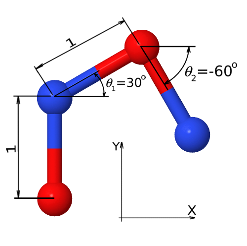
(a)

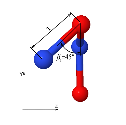
(b)

Figure 1: A schematic diagram of a sequence ABAB. (a) Projection of a structure with $\theta_{1}=30$, $\theta_{2}=-60$ and $\beta_{1}=0$ onto the XY-plane. (b) Projection of a structure with $\theta_{1}=30$, $\theta_{2}=-60$ and $\beta_{1}=45$ onto the ZY-plane.

2.2 Hydrophobic core

Information about a hydrophobic core, or a set of positions of the hydrophobic amino acids, is very useful for structure prediction in different methods. The authors in Backofen06 presented a constraint-based method. The key concept of this method is the ability to compute maximally compact hydrophobic cores. Information about hydrophobic cores was also used within stochastic algorithms for PFO. In Rashid16a ; Rashid16b ; Rashid13 a macro-mutation operator is incorporated into the genetic algorithm and applied to the three-dimensional face-centered cubic lattice. This operator compresses the conformation, and forms the hydrophobic-core quickly. The obtained results show that the macro-mutation operator improves the efficiency of the algorithm significantly.

3 Three-dimensional AB off-lattice model

A chain of amino acids can be represented with a unique amino acid sequence. From the amino acid sequence, it is possible to generate different conformations, which is also dependent on the model used. There are different models, such as a full atom, coarse-grained Kmiecik16 , AB off-lattice Stillinger93 and HP Hart2005 ; BoskovicHP16 . The full atom model is the most accurate and complex, and, as such, is computationally expensive. Although it is computationally expensive it was also used in the optimization process of the DE algorithm that was adapted for such a problem Rakhshani19 . Different coarse-grained models were designed to mitigate the computational complexity of the full atom model Kmiecik16 . The remaining two models, AB off-lattice and HP, are even more simplified and, as such, they are not very computationally expensive. The main purpose of these models is an analysis of different optimization algorithms. The three-dimensional AB off-lattice model is used in our paper, to demonstrate the efficiency of the proposed algorithm. Instead of 20 standard amino acids, this model uses only two different types of amino acids: $A$ – hydrophobic and $B$ – hydrophilic. Thus, an amino acid sequence is represented as a string $\vec{s}=\{s_{1},s_{2},...,s_{L}\}$, $s_{i}\in\{A,B\}$, where $A$ represents a hydrophobic, $B$ a hydrophilic amino acid, and $L$ the length of the sequence. The solution, or three-dimensional structure of an AB sequence, is defined by bond angles $\vec{\theta}=\{\theta_{1},\theta_{2},...,\theta_{L-2}\}$, torsional angles $\vec{\beta}=\{\beta_{1},\beta_{2},...,\beta_{L-3}\}$, and the unit-length chemical bond between two consecutive amino acids (see Fig. 1). The quality of the solution determines the energy value $E_{o}$, which is calculated using a simple trigonometric form of backbone bend potentials $E_{\text{bb}}(\vec{\theta})$ and a species-dependent Lennard-Jones 12,6 form of non-bonded interactions $E_{\text{lj}}(\vec{s},\vec{\theta},\vec{\beta})$, as shown in the following equation Stillinger93 :

$$\footnotesize E_{\text{o}}(\vec{s},\vec{\theta},\vec{\beta}) = E_{\text{bb}}(\vec{\theta})+E_{\text{lj}}(\vec{s},\vec{\theta},\vec{\beta})$$

$$E_{\text{\tiny bb}}(\vec{\theta}) = \frac{1}{4}\displaystyle\sum_{i=1}^{L-2}[1-cos(\theta_{i})]$$ (1)

$$E_{\text{\tiny lj}}(\vec{s},\vec{\theta},\vec{\beta}) = 4\displaystyle\sum_{i=1}^{L-2}\displaystyle\sum_{\text{{\it j}={\it i}+}2}^{L}[d(\vec{p}_{i},\vec{p}_{j})^{\text{--}12}\text{--}c(s_{i},s_{j})\cdot d(\vec{p}_{i},\vec{p}_{j})^{\text{--}6}]$$

where $\vec{p}_{i}$ and $\vec{p}_{j}$ represent the position of the amino acid within the three-dimensional space. These positions are determined, as shown in Fig. 1 and by the following equation:

$$\vec{p}_{i}=\begin{cases}\{0,0,0\}&\text{if}~{}i=1,\\ \{0,1,0\}&\text{if}~{}i=2,\\ \{cos(\theta_{1}),1+sin(\theta_{1}),0\}&\text{if}~{}i=3,\\ \{x_{i-1}+cos(\theta_{i-2})\cdot cos(\beta_{i-3}),\\ ~{}~{}y_{i-1}+sin(\theta_{i-2})\cdot cos(\beta_{i-3}),&\text{if 4}\leq i\leq L.\\ ~{}~{}z_{i-1}+sin(\beta_{i-3})\}\\ \end{cases}$$ (2)

In Eq. (3) $d(\vec{p}_{i},\vec{p}_{j})$ denotes the Euclidean distance between positions $\vec{p}_{i}$ and $\vec{p}_{j}$, while $c(s_{i},s_{j})$ determines the attractive, weak attractive or weak repulsive non-bonded interaction for the pair $s_{i}$ and $s_{j}$, as shown in the following equation:

$$c(s_{i},s_{j})=\begin{cases}1&\text{if }s_{i}=A\text{ and }s_{j}=A,\\ 0.5&\text{if }s_{i}=B\text{ and }s_{j}=B,\\ -0.5&\text{if }s_{i}\neq s_{j}.\\ \end{cases}$$

The objective of PFO within the context of an AB off-lattice model is to simulate the folding process, and to find the angles’ vector or conformation that minimizes the free-energy value: $\{\vec{\theta}^{*},\vec{\beta}^{*}\}=\operatorname*{\mathrm{arg\,min}}E_{o}(\vec{s},\vec{\theta},\vec{\beta})$. The described model takes into account the hydrophobic interactions which represent the main driving forces of a protein structure formation and, as such, still imitates its main features realistically Huang06 . Therefore, although this model is incomplete, it allows the development, testing, and comparison of various search algorithms.

4 Method

In order to include knowledge about the hydrophobic core to our algorithm, we have developed the two-phase optimization by using the DE algorithm. The optimization process is alternated between two phases until the stopping condition of the optimization process is satisfied, as shown in Fig. 2. The auxiliary fitness function is used in the first phase, which is responsible for forming conformations with a good hydrophobic core. When the stopping condition of the first phase is satisfied, the obtained population is forwarded to the second phase. The original fitness function is used in the second phase to locate solutions with the lowest energy value. When the second optimization phase is finished, the reinitialization is performed, and the optimization process continues with the first phase.

The main idea of the auxiliary fitness function is to allow the algorithm to form good hydrophobic-cores easily. For this purpose, it contains three expressions, as shown in Eq. (4).

$$E_{\text{x}}(\vec{s},\vec{\theta},\vec{\beta}) = E_{o}(\vec{s},\vec{\theta},\vec{\beta})+E_{\text{hc}}(\vec{s},\vec{\theta},\vec{\beta})+\lambda$$

$$E_{\text{hc}}(\vec{s},\vec{\theta},\vec{\beta}) = \sum_{i=1}^{L}d(\vec{p}_{i},\vec{c})\cdot h(s_{i})$$ (3)

$$h(s_{i}) = \begin{cases}1&\text{if }s_{i}=A,\\ 0&otherwise\end{cases}$$

$$\vec{c} = \frac{\sum_{i}^{N}{\vec{p}_{i}\cdot h(s_{i})}}{N_{A}};~{}~{}~{}N_{A}=\sum_{i}^{N}h(s_{i})$$

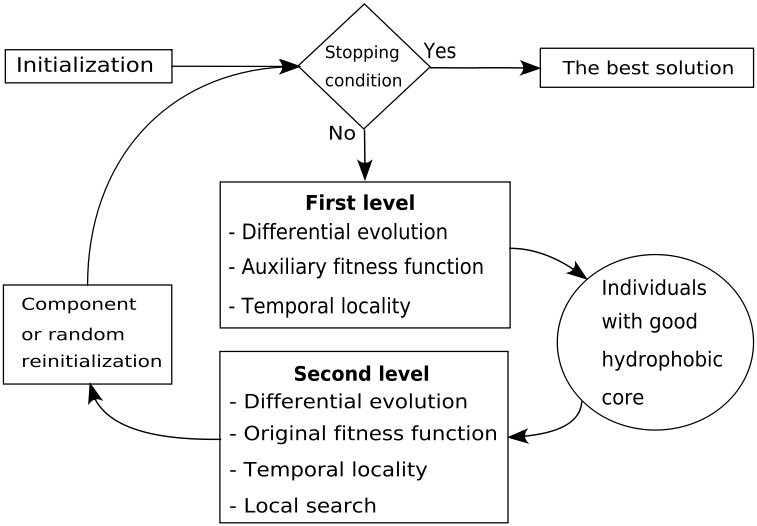
Figure 2: Two-phase optimization process of the proposed DE algorithm.

The first expression, $E_{o}$, represents the original fitness function, the second expression, $E_{hc}$, determines the quality of the hydrophobic core, while the third expression is a constant $\lambda$ that separates the fitness values between the first and second optimization phases. The quality of the hydrophobic core determines the sum of the Euclidean distances between all hydrophobic amino acids and their centroid $\vec{c}$. The value $\lambda$ ensures that the energy value $E_{x}$ in the first phase is always worse in comparison with the energy value $E_{o}$ in the second optimization phase. In this work, the value of $\lambda$ was set to 1,000. This value is large enough to make a gap between the fitness values of both optimization phases. This can be seen in the convergence graph (Fig. 5) where the red line represents the fitness values of the first phase, while the green line represents the fitness values of the second phase. The introduced gap between phase values allows the algorithm to update the global and local best vectors correctly without any additional mechanism.

4.1 Proposed algorithm

The proposed algorithm is based on our previous work BoskovicAB18 , and it was improved in such a way that the optimization process is divided into two phases. This algorithm is described in this Section, and it is shown in Figs. 3 and 4. The lines that include two-phase optimization into our algorithm are highlighted with a gray background.

1: procedure DE${}_{\text{2P}}$($\vec{s},\mathit{Np}$) 

2:    Initialize a population $P$ $\mathit{firstPhase}=\text{\bf true}$$\{\vec{x}_{i},F_{i}=0.5,\mathit{Cr}_{i}=0.9,e_{i}=$$E_{x}$($\vec{s},\vec{x_{i}}$)$\}\in P$ $x_{i,j}=-\pi+2\cdot\pi\cdot\mathit{rand}_{[0,1]}$ $i=1,2,...,\mathit{Np};j=1,2,...,D;D=2\cdot$ $\mathit{length}$($\vec{s}$) - 5$\{\vec{x}_{b},e_{b}\}=\{\vec{x}_{b}^{l},e_{b}^{l}\}=\{\vec{x}_{b}^{p},e_{b}^{p}\}=$ BEST($P$)

3:    while stopping criteria is not met do

4:       for $i=1$ to $\mathit{Np}$ do

5:          if $\mathit{rand}_{[0,1]}<0.1$ then $F=0.1+0.9\cdot\mathit{rand}_{[0,1]}$ else $F=F_{i}$ end if

6:          if $\mathit{rand}_{[0,1]}<0.1$ then $\mathit{Cr}=\mathit{rand}_{[0,1]}$ else $\mathit{Cr}=\mathit{Cr}_{i}$ end if

7:          do $r_{{}_{1}}\text{=}\mathit{rand}_{\{1,\mathit{Np}\}}$ while $r_{{}_{1}}\text{=}i$ end do

8:          do $r_{{}_{2}}\text{=}\mathit{rand}_{\{1,\mathit{Np}\}}$ while $r_{{}_{2}}\text{=}i~{}\text{\bf or}~{}r_{{}_{2}}\text{=}r_{{}_{1}}$ end do

9:          $j_{\mathit{rand}}=\mathit{rand}_{\{1,\mathit{D}\}}$

10:          for $j=1$ to $D$ do

11:             if $\mathit{rand}_{[0,1]}<\mathit{Cr}~{}\text{\bf or }~{}j=j_{\mathit{rand}}$ then

12:                $u_{j}=x_{b,j}+F\cdot(x_{r_{1},j}-x_{r_{2},j})$

13:                if $u_{j}\leq\text{-}\pi$ then $u_{j}\text{\,=\,}2\cdot\pi+u_{j}$ end if

14:                if $u_{j}>\pi$ then $u_{j}\text{\,=\,}2\cdot(\text{-}\pi)+u_{j}$ end if

15:             else

16:                $u_{j}=x_{i,j}$

17:             end if

18:          end for

19:          if $\mathit{firstPhase}$ then

20:             $e_{u}=$$E_{x}$($\vec{s},\vec{u}$) // Auxiliary fitness function

21:          else

22:             $e_{u}=$$E_{o}$($\vec{s},\vec{u}$) // Original fitness function

23:          end if

24:          if $e_{u}\leq e_{i}$ then

25:             // Temporal locality

26:             for $j=1$ to $D$ do

27:                $u^{*}_{j}=x_{b,j}+0.5\cdot(u_{j}-x_{i,j})$

28:                if $u^{*}_{j}\leq\text{-}\pi$ then $u^{*}_{j}\text{\,=\,}2\cdot\pi+u^{*}_{j}$ end if

29:                if $u^{*}_{j}>\pi$ then $u^{*}_{j}\text{\,=\,}2\cdot(\text{-}\pi)+u^{*}_{j}$ end if

30:             end for

31:             if $\mathit{firstPhase}$ then

32:                $e^{*}_{u}=$$E_{x}$($\vec{s},\vec{u}^{*}$) // Auxiliary fitness function

33:             else

34:                $e^{*}_{u}=$$E_{o}$($\vec{s},\vec{u}^{*}$) // Original fitness function

35:             end if

36:             if $e^{*}_{u}\leq e_{u}$ then

37:                $\{\vec{x_{i}},F_{i},\mathit{Cr_{i}},e_{i}\}=\{u^{*},F,\mathit{Cr},e^{*}_{u}\}$

38:             else

39:                $\{\vec{x_{i}},F_{i},\mathit{Cr_{i}},e_{i}\}=\{u,F,\mathit{Cr},e_{u}\}$

40:             end if

41:             if not $\mathit{firstPhase}$ then

42:                // Local Search

43:                for $n=2$ to $L-1$ do

44:                   $\theta_{n\text{-}1}=\mathit{rand}_{[0,1]}\cdot(x^{p}_{b,n\text{-}1}-x_{i,n\text{-}1})$

45:                   $\beta_{n\text{-}2}=\mathit{rand}_{[0,1]}\cdot(x^{p}_{b,n+(L\text{-}4)}-x_{i,n+(L\text{-}4)})$

46:                   {${\vec{v},e_{v}}\}=$ LOCAL_MOVEMENT($\vec{x}^{p}_{b},n,\theta_{n\text{-}1},\beta_{n\text{-}2}$)

47:                   if $e_{v}\leq e_{b}$ then $\{\vec{x}^{p}_{b},e^{p}_{i}\}=\{\vec{v},e_{v}\}$ end if

48:                end for

49:             end if

50:          end if

51:       end for

52:       $\{\vec{x}_{b}^{p},e_{b}^{p}\}=$ BEST($P$)

53:       if $e_{b}^{p}\leq e_{b}$ then $\{\vec{x}_{b},e_{b}\}=\{\vec{x}_{b}^{p},e_{b}^{p}\}$ end if

54:       REINITIALIZATION($\{\vec{x}_{b}^{p},e_{b}^{p}\}$,$\{\vec{x}_{b}^{l},e_{b}^{l}\}$,$P$,$\mathit{firstPhase}$ )

55:    end while

56:    return  $\{\vec{x}_{b},e_{b}\}$

57: end procedure

Figure 3: The proposed DE${}_{\text{2P}}$ algorithm.

The optimization begins with initialization (line 2 in Fig. 3). Each iteration of the $\mathit{while}$ loop (line 3) represents one generation of the evolutionary process. In one generation the DE/best/1/bin strategy is performed for each population’s vector {$\vec{x}_{1}$, $\vec{x}_{2}$, …, $\vec{x}_{Np}$} for creating a trial vector $\vec{u}$ (lines 5 – 18). The values of control parameters are set by using the jDE algorithm Brest06 . Each vector is a D-dimensional vector that contains real coded bond $\theta$ and torsional $\beta$ angles:

$$\vec{x}_{i}=\{\theta_{i,1},\theta_{i,2}\,...,\theta_{i,L-2},\beta_{i,1},\beta_{i,2},...,\beta_{i,L-3}\},$$

where $D=2\cdot L-5$ is the dimension of the problem, and $x_{i,j}\in[-\pi,\pi]$. The variable $\mathit{firstPhase}$ determines the current optimization phase. The trial vector $\vec{u}$ is evaluated according to the value of this variable, as shown in line 19. If the trial vector is better than the corresponding vector from the population $\vec{x}_{i}$, then yet another trial vector $\vec{u^{*}}$ is generated using temporal locality (lines 24 – 30), and evaluated according to the current optimization phase. The second trial vector $\vec{u^{*}}$ is generated by using the promising movement that is added to the best population vector. In lines 37 and 39, the corresponding population vector is replaced by the better trial vector. The main goal of the first phase is to form good hydrophobic cores, and it is not necessary to reach very accurate solutions. Therefore, the local search is not used in this phase, as shown in line 41. The local search includes a local movement mechanism that allows efficient evaluation of neighborhood vectors which have moved locally only two consecutive monomers, while all remaining monomers are unchanged. Thus, this mechanism is only used in the second optimization phase for performing an accurate search.

1: procedure REINITIALIZATION($\{\vec{x}_{b}^{p},e_{b}^{p}\},\{\vec{x}_{b}^{l},e_{b}^{l}\},P,\mathit{firstPhase}$) 

2:    if $e_{b}^{p}\leq e_{b}^{l}$ then $\{\vec{x}_{b}^{l},e_{b}^{l}\}=\{\vec{x}_{b}^{p},e_{b}^{p}\}$ end if

3:    if  $\mathit{firstPhase}$  then

4:       if $\vec{x}_{b}^{l}$ is unchanged for at least $H_{c}\cdot D$ evaluations within the first phase then

5:          $\mathit{firstPhase}={\bf false}$

6:       end if

7:    else

8:       if $\vec{x}_{b}^{l}$ is unchanged for at least $P_{b}\cdot D$ evaluations within the second phase then

9:          // Component reinitialization

10:          $\vec{x}_{i}=$ RANDOM($\vec{x}_{b}^{l},C$);    $i=1,2,...,\mathit{Np}$

11:          $\{\vec{x}_{b}^{p},e_{b}^{p}\}=$ BEST($P$)

12:          $\mathit{firstPhase}={\bf true}$

13:       end if

14:       if $\vec{x}_{b}^{l}$ is unchanged for $L_{b}\cdot D$ component reinitializations then

15:          // Random reinitialization

16:          $\vec{x}_{i}=$ RANDOM() ;    $i=1,2,...,\mathit{Np}$

17:          $\{\vec{x}_{b}^{l},e_{b}^{l}\}=\{\vec{x}_{b}^{p},e_{b}^{p}\}=$ BEST($P$)

18:          $\mathit{firstPhase}={\bf true}$

19:       end if

20:    end if

21: end procedure

Figure 4: The reinitialization mechanism.

The first generation belongs to the first optimization phase. The reinitialization method is performed at the end of each generation, and it is responsible for reinitializations and determining the optimization phase. We have defined three different best vectors BoskovicAB18 . The best population vector $\vec{x}_{b}^{p}$ is the best vector in the current population, the local best vector $\vec{x}_{b}^{l}$ is the best vector among all similar vectors, and the global best vector $\vec{x}_{b}^{g}$ is the best vector obtained within the evolutionary process. How long the local best vector stayed unchanged within the optimization process and the value of control parameters $H_{c},L_{b}$, and $P_{b}$, determine the reinitialization and optimization phase. The algorithm switches to the second optimization phase when $\vec{x}_{b}^{l}$ is unchanged for at least $H_{c}\cdot D$ evaluations within the first optimization phase. The component reinitialization is performed when $\vec{x}_{b}^{l}$ is unchanged for at least $P_{b}\cdot D$ evaluations within the second optimization phase, while the random reinitialization is performed when the $\vec{x}_{b}^{l}$ is unchanged for at least $L_{b}\cdot D$ component reinitializations. In this way, the component reinitialization increases the likelihood of finding a good similar solution that is different from the already found good solution in only a few components. The parameter $C$ determines the number of components that are different between $\vec{x}_{b}^{l}$ and vectors generated by component reinitialization (line 10). On the other hand, random reinitialization guides the search process to unexplored search space regions. For a detailed description of all mechanisms of our previous work and its influence to the algorithm’s efficiency, we refer readers to BoskovicAB16 and BoskovicAB18 .

5 Experiments

The DE${}_{\text{2P}}$ algorithm was implemented by using SPSE (Stochastic Problem Solving Environment), compiled with a GNU C++ compiler 5.4.0, and executed using an Intel Core i5 computer with 3.2 GHz CPU and 16 GB RAM under Linux Mint 18.3 Sylvia and a grid environment (Slovenian Initiative for National Grid). The grid environment was configured to use AMD Opteron 6272 processor with clock speed of 2.1 GHz, cache of 2 MB, and main memory of 128 GB assigned to 64 cores. The SPSE environment allows for rapid development and testing of stochastic algorithms for different problems in an efficient way. The console and web interface are available within this environment. By using the web interface, we developed a web application that is available at https://spse.feri.um.si, where the proposed algorithm can be tested and the optimization process is visualized. In order to evaluate the efficiency of the proposed algorithm, we used a set of amino acid sequences, as shown in Table 2. This set includes 18 real peptide sequences from the Protein Data Bank database, and 5 Fibonacci sequences. The K-D method Mount01 is used to transform the real peptide sequences to the AB sequences. In this method, the amino acids isoleucine, valine, proline, leucine, cysteine, methionine, alanine, and glycine, are transformed to hydrophobic ones (A), while aspartic acid, glutamic acid, histidine, phenylalanine, lysine, asparagine, glutamine, arginine, serine, threonine, tryptophan, and tyrosine to hydrophilic ones (B). The selected sequences have different lengths, which enabled us to analyze the algorithm with the three stopping conditions. The quality of the solution ($E_{t}$), or the target scenario, was used for short sequences, while the limited amount of solution evaluation ($\mathit{NSE_{\mathit{lmt}}}$) and runtime ($\mathit{t_{\mathit{lmt}}}$) were used for long sequences. The used sequences can also be found in many papers, and, therefore, allow us to compare the proposed algorithm with different algorithms.

Table 3 summarizes the expressions that were used in our experiments. Note that all energy values are multiplied by $\text{-}1$, which means that all reported energy values are positive, and higher values are better. $N_{r}=30$ independent runs were performed when the proposed algorithm was compared with the state-of-the-art algorithms. In all other experiments, $N_{r}=100$ independent runs were used. In the target scenario, experimental results of $\mathit{NSE}$ have near-exponential or near-geometric distribution. Under such distributions, and with $N_{r}=N_{succ}=100$ runs, a reliable rule-of-thumb estimates a 95% confidence interval as follows:

Table 1: Mean ranks for different settings of the following parameters: $P_{b}$, $L_{b}$, $C$, and $H_{c}$.

$\mathit{r_{mean}}$	$P_{b}$	$L_{b}$	$C$	$H_{c}$
3.11	20	20	10	35
3.11	20	25	10	35
3.22	15	20	10	35
4.11	20	20	10	40
4.44	20	15	10	35
5.33	25	20	10	35
5.78	20	20	10	30
7.11	20	20	15	35
8.67	20	20	5	35

Table 2: Details of amino acid sequences used in experiments.

label	$L$	$D$	sequence
1BXP	13	21	ABBBBBBABBBAB
1CB3	13	21	BABBBAABBAAAB
1BXL	16	27	ABAABBAAAAABBABB
1EDP	17	29	ABABBAABBBAABBABA
2ZNF	18	31	ABABBAABBABAABBABA
1EDN	21	37	ABABBAABBBAABBABABAAB
2H3S	25	45	AABBAABBBBBABBBABAABBBBBB
1ARE	29	53	BBBAABAABBABABBBAABBBBBBBBBBB
2KGU	34	63	ABAABBAABABBABAABAABABABABABAAABBB
1TZ4	37	69	BABBABBAABBAAABBAABBAABABBBABAABBBBBB
1TZ5	37	69	AAABAABAABBABABBAABBBBAABBBABAABBABBB
1AGT	38	71	AAAABABABABABAABAABBAAABBABAABBBABABAB
1CRN	46	87	BBAAABAAABBBBBAABAAABABAAAABBBAAAAAAAABAAABBAB
2KAP	60	115	BBAABBABABABABBABABBBBABAABABAABBBBBBABBBAABAAABBABBABBAAAAB
1HVV	75	145	BAABBABBBBBBAABABBBABBABBABABAAAAABBBABAABBABBBABBAABBABBAABBBBBAABBBBBABBB
1GK4	84	163	ABABAABABBBBABBBABBABBBBAABAABBBBBAABABBBABBABBBAABBABBBBBAABABAAABABAABBBBAABABBBBA
1PCH	88	171	ABBBAAABBBAAABABAABAAABBABBBBBABAAABBBBABABBAABAAAAAABBABBABABABABBABBAABAABBBAABBAAABA
2EWH	98	191	AABABAAAAAAABBBAAAAAABAABAABBAABABAAABBBAAAABABAAABABBAAABAAABAAABAABBAABAAAAABAAABABBBABBAAABAABA
F13	13	21	ABBABBABABBAB
F21	21	37	BABABBABABBABBABABBAB
F34	34	63	ABBABBABABBABBABABBABABBABBABABBAB
F55	55	105	BABABBABABBABBABABBABABBABBABABBABBABABBABABBABBABABBAB
F89	89	173	ABBABBABABBABBABABBABABBABBABABBABBABABBABABBABBABABBABABBABBABABBABBABABBABABBABBABABBAB

Table 3: Summary of expressions that were used in experiments.

Expression	Brief description
$N_{r}$	the number of runs
$E_{i}$	the energy value ($E_{o}$) of $i$-th run
$E_{\mathit{mean}}=\frac{\sum_{i=1}^{N_{r}}E_{i}}{N_{r}}$	the mean energy value
$E_{\mathit{best}}=\mathit{max}\{E_{1},E_{2},...,E_{N_{r}}\}$	the best energy value
$E_{\mathit{std}}=\sqrt{\frac{\sum_{i=1}^{N_{r}}(E_{i}-E_{\mathit{mean}})^{2}}{N_{r}-1}}$	the standard deviation of energy values
$E_{\mathit{t}}$	the energy or target value to be reached
$N_{\mathit{succ}}$	the number of runs where the target value $E_{t}$ is reached
$S_{r}=\frac{N_{succ}}{N_{r}}$	the success ratio
$\mathit{NSE}_{i}$	the number of solution evaluations for $i$-th run
$\mathit{NSE}_{\mathit{mean}}=\frac{\sum_{i=1}^{N_{\mathit{succ}}}\mathit{NSE}_{i}}{N_{\mathit{succ}}}$	the mean number of solution evaluation for all $N_{\mathit{succ}}$ runs

Expression	Brief description
$t_{i}$	the runtime of $i$-th run
$t_{\mathit{mean}}=\frac{\sum_{i=1}^{N_{r}}t_{i}}{N_{r}}$	the mean runtime for $N_{r}$ runs
$r_{i}$	the setting rank of $i$-th sequence
$N_{s}$	the number of sequences
$r_{\mathit{mean}}=\frac{\sum_{i=1}^{N_{s}}r_{i}}{N_{s}}$	the mean rank
$\mathit{NSE}_{\mathit{lmt}}$	the number of solution evaluations limit for one run
$\mathit{t}_{\mathit{lmt}}$	the runtime limit for one run
$\mathit{NSE}^{1},\mathit{NSE}^{2}$	the number of solution evaluations within the first and second optimization phase
$t^{1},t^{2}$	the runtime within the first and second optimization phase

$$\begin{split}\mathit{\mathit{NSE}}_{95}\approx~{}&[(1-\frac{1.96}{\sqrt{N_{r}}})\cdot\mathit{NSE}_{\mathit{mean}},\\ &(1+\frac{1.96}{\sqrt{N_{r}}})\cdot\mathit{NSE}_{\mathit{mean}}]\\ \approx~{}&[0.8\cdot\mathit{NSE}_{\mathit{mean}},1.2\cdot\mathit{NSE}_{\mathit{mean}}].\end{split}$$ (4)

Table 4: The ranked ($r_{i}$) control parameter settings ($P_{b},L_{b},C,H_{c}$). The population size $Np$ and the number of independent runs $N_{r}$ were set to 100. The stopping conditions were the target energy $E_{t}$ and limit of solution evaluations $\mathit{NSE}_{\mathit{lmt}}=2\cdot 10^{11}$.

$r_{1}$	$P_{b}$	$L_{b}$	$C$	$H_{c}$	$\mathit{NSE_{mean}}$
1	15	20	10	35	5.371e+06
2	20	25	10	35	5.443e+06
3	20	15	10	35	5.509e+06
4	20	20	10	35	5.653e+06
5	20	20	10	30	5.874e+06
6	25	20	10	35	6.076e+06
7	20	20	10	40	6.131e+06
8	20	20	15	35	6.386e+06
9	20	20	5	35	2.151e+07

(a) F13, $\mathit{E_{t}}=6.9961$

$r_{2}$	$P_{b}$	$L_{b}$	$C$	$H_{c}$	$\mathit{NSE_{mean}}$
1	20	20	10	30	5.930e+06
2	20	20	15	35	6.079e+06
3	20	20	10	35	6.563e+06
4	20	20	10	40	6.790e+06
5	20	25	10	35	6.810e+06
6	20	15	10	35	7.037e+06
7	25	20	10	35	7.055e+06
8	15	20	10	35	7.593e+06
9	20	20	5	35	2.498e+07

(b) 1CB3, $\mathit{E_{t}}=8.4589$

$r_{3}$	$P_{b}$	$L_{b}$	$C$	$H_{c}$	$\mathit{NSE_{mean}}$
1	15	20	10	35	1.935e+07
2	20	25	10	35	1.937e+07
3	20	20	10	35	2.001e+07
4	20	20	15	35	2.014e+07
5	20	20	10	40	2.043e+07
6	20	15	10	35	2.137e+07
7	25	20	10	35	2.288e+07
8	20	20	10	30	2.400e+07
9	20	20	5	35	9.956e+07

(c) 1BXP, $\mathit{E_{t}}=5.6104$

$r_{4}$	$P_{b}$	$L_{b}$	$C$	$H_{c}$	$\mathit{NSE_{mean}}$
1	15	20	10	35	5.759e+08
2	20	20	10	35	5.835e+08
3	20	25	10	35	6.129e+08
4	20	20	10	30	6.727e+08
5	20	20	10	40	6.840e+08
6	25	20	10	35	7.216e+08
7	20	15	10	35	8.349e+08
8	20	20	15	35	1.317e+09
9	20	20	5	35	5.748e+09

(d) 1BXL, $\mathit{E_{t}}=17.3962$

$r_{5}$	$P_{b}$	$L_{b}$	$C$	$H_{c}$	$\mathit{NSE_{mean}}$
1	20	25	10	35	2.579e+08
2	20	20	10	40	2.615e+08
3	20	20	10	35	2.687e+08
4	20	15	10	35	2.791e+08
5	15	20	10	35	2.806e+08
6	25	20	10	35	2.871e+08
7	20	20	10	30	2.932e+08
8	20	20	15	35	4.820e+08
9	20	20	5	35	1.012e+09

(e) 1EDP, $\mathit{E_{t}}=15.0092$

$r_{6}$	$P_{b}$	$L_{b}$	$C$	$H_{c}$	$\mathit{NSE_{mean}}$
1	15	20	10	35	4.788e+08
2	20	15	10	35	5.141e+08
3	25	20	10	35	5.793e+08
4	20	20	10	35	5.972e+08
5	20	25	10	35	5.969e+08
6	20	20	10	40	6.118e+08
7	20	20	10	30	6.230e+08
8	20	20	15	35	9.570e+08
9	20	20	5	35	2.531e+09

(f) 2ZNF, $\mathit{E_{t}}=18.3402$

$r_{7}$	$P_{b}$	$L_{b}$	$C$	$H_{c}$	$\mathit{NSE_{mean}}$
1	20	15	10	35	1.629e+09
2	20	25	10	35	1.649e+09
3	20	20	10	35	1.702e+09
4	25	20	10	35	1.833e+09
5	20	20	10	40	1.836e+09
6	20	20	10	30	1.898e+09
7	15	20	10	35	2.089e+09
8	20	20	5	35	4.776e+09
9	20	20	15	35	8.858e+09

(g) F21, $\mathit{E_{t}}=16.5544$

$r_{8}$	$P_{b}$	$L_{b}$	$C$	$H_{c}$	$\mathit{NSE_{mean}}$
1	20	20	10	40	5.658e+09
2	15	20	10	35	6.062e+09
3	25	20	10	35	6.458e+09
4	20	25	10	35	6.924e+09
5	20	20	10	35	7.366e+09
6	20	15	10	35	8.589e+09
7	20	20	10	30	8.693e+09
8	20	20	5	35	1.522e+10
9	20	20	15	35	3.296e+10

(h) 1EDN, $\mathit{E_{t}}=21.4703$

$r_{9}$	$P_{b}$	$L_{b}$	$C$	$H_{c}$	$\mathit{NSE_{mean}}$
1	20	20	10	35	1.971e+10
2	20	20	10	40	2.100e+10
3	15	20	10	35	2.145e+10
4	20	25	10	35	2.179e+10
5	20	15	10	35	2.352e+10
6	25	20	10	35	2.396e+10
7	20	20	10	30	2.454e+10
8	20	20	15	35	-
8	20	20	5	35	-

(i) 2H3S, $\mathit{E_{t}}=21.1519$

5.1 Parameter settings

Although the two-phase optimization introduces only one new parameter $H_{c}$, the algorithm works quite differently than the previous one. Therefore, in this Section, we will show the influence of the four control parameters $P_{b}$, $L_{b}$, $C$, and $H_{c}$ to the algorithm’s efficiency while the population size $N_{p}$ was set to 100 according to the experiment in BoskovicAB16 . In our analysis of four parameters, the target scenario ($E_{t}$) was used on short sequences. For each sequence, we used $N_{s}=9$ different settings and the obtained results are shown in Table 4. Entries that are shown as ’-’ imply that the algorithm could not reach the target value $E_{t}$ in all the runs within the budget of $2\cdot 10^{11}$ solution evaluations. The recommended settings and their results are shown in bold typeface. From the displayed results, we can see that each sequence has its optimal setting, but it is still possible to select a good setting for all sequences. For this purpose, settings were ranked in Table 4 and mean rank $r_{\mathit{mean}}$ was calculated for each setting, as shown in Table 1. Two settings obtained the best $r_{\mathit{mean}}=3.11$. We selected the following values $P_{b}=20,L_{b}=20,C=10$, $Hc=35$, and $N_{p}=100$ as a good setting, since this setting obtained the best result on the largest sequence 2H3S. Therefore, this setting is used in all the remaining experiments. From the displayed results, we can also see that parameter $C$ is the most sensitive parameter. The best rank was obtained for the setting with $C=10$, while the worst ranks were obtained for settings with $C=5$ and $C=15$. This can also be observed in Table 4(i), where the best result was obtained with $C=10$, while for settings with $C=5$ and $C=15$ the algorithm could not reach the target energy value $E_{t}$ in all runs. Similar relationships of these parameter values can be observed for most sequences in Table 4.

Table 5: Comparison of the DE${}_{\text{lscr}}$, DE${}_{\text{lscr}}$^∗, and DE${}_{\text{2P}}$ algorithms with $N_{r}=100$ and $\mathit{NSE}_{\mathit{lmt}}=10^{6}$.

Label	L	DE${}_{\text{lscr}}$				DE${}_{\text{lscr}}$*				DE${}_{\text{2P}}$
		$E_{\mathit{mean}}$	$E_{\mathit{std}}$	p-value		$E_{\mathit{mean}}$	$E_{\mathit{std}}$	p-value		$E_{\mathit{mean}}$	$E_{\mathit{std}}$
F13	13	4.5648	0.9986	6.8001e-27		6.2744	0.2525	5.7081e-19		6.6551	0.2330
1CB3	13	6.2329	2.0785	4.8569e-17		7.3615	0.3759	4.0492e-23		8.0308	0.3268
1BXP	13	4.4583	0.1995	5.9807e-33		4.9028	0.3131	8.9531e-11		5.1683	0.2028
1BXL	16	14.5008	2.0514	1.6152e-16		15.3518	0.4369	8.3531e-18		15.9518	0.4941
1EDP	17	11.2560	2.4148	2.7825e-17		13.1234	0.5382	1.9038e-11		13.6529	0.4100
2ZNF	18	12.5251	3.0289	6.1052e-27		15.8738	0.5498	8.7550e-14		16.4476	0.7285
F21	21	10.0228	1.7237	1.9620e-25		13.4101	0.9603	0.8517e-00		13.4152	1.3192
1EDN	21	14.0150	3.3468	1.8642e-23		18.0786	0.6656	1.1487e-05		18.4635	0.9433
2H3S	25	12.4696	2.5977	1.6222e-24		16.2500	1.1672	0.0065e-00		16.7300	1.2836

Table 6: Comparison of the following algorithms: DE${}_{\text{2P}}$ and DE${}_{\text{lscr}}$. The shown $\mathit{NSE_{coef}}=\frac{\mathit{NSE_{mean}}(\text{DE${}_{\text{lscr}}$})}{\mathit{NSE_{mean}}(\text{DE${}_{\text{2P}}$})}$ and $\mathit{t_{coef}}=\frac{\mathit{t_{mean}}(\text{DE${}_{\text{lscr}}$})}{\mathit{t_{mean}}(\text{DE${}_{\text{2P}}$})}$ represent the relationship between corresponding statistics.

Label	$L$	$D$	$E_{t}$	DE${}_{\text{lscr}}$ BoskovicAB18					DE${}_{\text{2P}}$				$\mathit{NSE_{coef}}$	$\mathit{t_{coef}}$	p-value
				$\mathit{NSE_{mean}}$	$\mathit{NSE_{std}}$	$\mathit{t_{mean}}$ [sec]			$\mathit{NSE_{mean}}$	$\mathit{NSE_{std}}$	$\mathit{t_{mean}}$ [sec]
F13	13	21	6.9961	8.92e+07	8.52e+07	110.54			5.65e+06	6.33e+06	6.35		15.8	17.4	1.14e-28
1CB3	13	21	8.4589	3.61e+07	4.26e+07	44.47			6.56e+06	6.40e+06	7.50		5.5	5.9	1.84e-14
1BXP	13	21	5.6104	1.56e+09	1.68e+09	1,965.08			2.00e+07	1.94e+07	22.00		78.0	89.3	3.22e-33
1BXL	16	27	17.3962	1.24e+10	1.24e+10	16,544.45	*		5.84e+08	6.06e+08	796.22		21.2	20.8	1.66e-30
1EDP	17	29	15.0092	4.58e+09	4.21e+09	7,272.60	*		2.69e+08	2.88e+08	394.28		17.0	18.4	1.05e-28
2ZNF	18	31	18.3402	2.10e+09	1.92e+09	3,098.81	*		5.97e+08	5.73e+08	948.52		3.5	3.3	2.36e-13
F21	21	37	16.5544	-	-	-			1.70e+09	1.74e+09	3,228.19		-	-	-
1EDN	21	37	21.4703	-	-	-			7.37e+09	6.65e+09	13,962.33	*	-	-	-
2H3S	25	45	21.1519	-	-	-			1.97e+10	1.98e+10	45,721.34	*	-	-	-

5.2 Auxiliary fitness function

An auxiliary fitness function includes knowledge about the quality of the hydrophobic core. This knowledge is crucial for the efficient optimization process. To demonstrate this advantage of the auxiliary fitness function, we compared DE${}_{\text{lscr}}$, DE${}_{\text{lscr}}$^∗, and DE${}_{\text{2P}}$. DE${}_{\text{lscr}}$ (Differential Evolution Extended with Local Search and Component Reinitialization) BoskovicAB18 is our algorithm, that does not have two-phase optimization while DE${}_{\text{lscr}}$^∗ is the same algorithm as DE${}_{\text{lscr}}$, but instead of the original fitness function, it uses auxiliary fitness function throughout the entire optimization process. Only the final population is evaluated with the original fitness function, and the best vector is returned as a result of optimization. In this experiment, 100 independent runs were performed for each algorithm, and the stopping condition was $\mathit{NSE}_{\mathit{lmt}}=10^{6}$. From the shown results in Table 5, we can observe that the DE${}_{\text{lscr}}$^∗ obtained better results in comparison with the DE${}_{\text{lscr}}$ for all sequences. This demonstrates that the auxiliary fitness function has a good influence on the algorithm’s efficiency. We can also observe that the best results (shown in boldface) are obtained with DE${}_{\text{2P}}$ which demonstrates that the two-phase optimization improves the algorithm’s efficiency additionally. This conclusion is also supported by the Mann-Whitney $U$ test. With this test, we verify the equality of the medians between the energy values of the two algorithms. The shown $p$-values in Table 5 represents comparison between of DE${}_{\text{lscr}}$ and DE${}_{\text{lscr}}$^∗ with DE${}_{\text{2P}}$. From these results, it is evident that the statistically significant difference was identified at the 0.05 level of significance ($p$-value $<$ 0.05) in almost all cases. Only for sequence F21, there was no significant difference between the results of the DE${}_{\text{2P}}$ and DE${}_{\text{lscr}}$^∗ algorithms.

5.3 Two-phase optimization

Two-phase optimization was designed to increase the quality of the hydrophobic cores and, consequently, improve the efficiency of the algorithm. In order to demonstrate these advantages, the algorithm with two-phase optimization DE${}_{\text{2P}}$ was compared with the algorithm DE${}_{\text{lscr}}$. Within this comparison, the algorithms were compared by using two scenarios. In the first scenario, the following stopping conditions were used on the small sequences: $E_{t}=$ best-known energy value and $\mathit{NSE}_{\mathit{lmt}}=10^{11}$. The results of this scenario are shown in Table 6, and entries that are shown as ’-’ imply that the algorithm could not reach the target value $E_{t}$ in all runs. Values marked with the * are obtained by using the grid environment, and in these cases $t_{\mathit{mean}}=\frac{\mathit{NSE}_{\mathit{mean}}}{v_{\mathit{mean}}}$. Here, $v_{\mathit{mean}}$ represents the obtained mean speed of three independent runs on our test computer with $t_{\mathit{lmt}}=3600$ seconds. All other results are obtained on our test computer. From these results, it is evident that DE${}_{\text{2P}}$ obtained significantly better results in comparison with DE${}_{\text{lscr}}$, the distribution of the $\mathit{NSE}$ is near-exponential or near-geometric, because $\mathit{NSE}_{\mathit{mean}}\approx\mathit{NSE}_{\mathit{std}}$, and DE${}_{\text{2P}}$ obtained $S_{r}=1$ for all sequences with up to 25 monomers, while DE${}_{\text{lscr}}$ only for sequences with up to 18 monomers. The $\mathit{NSE}_{\mathit{coef}}$ and $t_{\mathit{coef}}$ were calculated for sequences where $S_{r}=1$. These coefficients represent the relationship between the algorithm’s results for $\mathit{NSE}_{\mathit{mean}}$ and $t_{\mathit{mean}}$. We can see that these statistics of DE${}_{\text{2P}}$ are decreased from 3.5 to 78 times, and from 3.3 to 89.3 times in comparison with DE${}_{\text{lscr}}$. A statistically significant difference at the 0.05 level of significance for $NSE_{\mathit{mean}}$ can also be observed, because 95% confidence intervals (see Eq. 4) do not overlap. Additionally, by using the Mann-Whitney $U$ test we verify the equality of the medians between the $NSE$ of algorithms. The shown $p$-values in Table 6 indicate that significant difference was identified at the 0.05 level of significance in all the cases. From these results, we can conclude that the two-phase optimization improves the efficiency of the algorithm for small sequences significantly.

Table 7: The obtained results for DE${}_{\text{2P}}$ and DE${}_{\text{lscr}}$ within a runtime limit $t_{\mathit{lmt}}=4$ days for $N_{r}=100$ independent runs for each sequence.

Label	$L$	DE${}_{\text{2P}}$					DE${}_{\text{lscr}}$ BoskovicAB18				p-value
		$\mathit{E_{best}}$	$\mathit{E_{mean}}$	$\mathit{E_{std}}$	$\mathit{S_{r}}$		$\mathit{E_{best}}$	$\mathit{E_{mean}}$	$\mathit{E_{std}}$	$\mathit{S_{r}}$
1BXP	13	5.6104	5.6104	0.0000	1.00		5.6104	5.6104	0.0000	1.00	-
1CB3	13	8.4589	8.4589	0.0000	1.00		8.4589	8.4589	0.0000	1.00	-
1BXL	16	17.3962	17.3962	0.0000	1.00		17.3962	17.3962	0.0000	1.00	-
1EDP	17	15.0092	15.0092	0.0000	1.00		15.0092	15.0092	0.0000	1.00	-
2ZNF	18	18.3402	18.3402	0.0000	1.00		18.3402	18.3402	0.0000	1.00	-
1EDN	21	21.4703	21.4703	0.0000	1.00		21.4703	21.3669	0.0431	0.07	5.76e-36
2H3S	25	21.1519	21.1488	0.0167	0.96		21.1519	20.9956	0.0995	0.19	2.39e-27
1ARE	29	25.2883	24.9863	0.1455	0.03		25.2800	24.5444	0.1718	0.00	1.59e-31
2KGU	34	53.6756	52.9066	0.1957	0.01		52.7165	51.7233	0.3829	0.00	4.26e-34
1TZ4	37	43.1890	42.7879	0.2478	0.03		43.0229	41.8734	0.4285	0.00	1.28e-29
1TZ5	37	50.2703	49.7110	0.2238	0.02		49.3868	48.6399	0.3292	0.00	6.98e-34
1AGT	38	66.2973	65.5231	0.2948	0.01		65.1990	64.1285	0.4173	0.00	6.68e-34
1CRN	46	95.3159	93.7138	0.5536	0.01		92.9853	89.8223	0.6514	0.00	3.36e-34
2KAP	60	89.5013	87.6293	0.8335	0.01		85.5099	83.1503	1.0041	0.00	2.56e-34
1HVV	75	101.6018	98.0730	1.3038	0.01		95.4475	91.4531	1.9215	0.00	2.80e-34
1GK4	84	112.3674	108.2822	1.9783	0.01		106.4190	99.6704	3.0377	0.00	2.95e-33
1PCH	88	166.7194	161.4182	2.1279	0.01		156.5250	153.1003	2.7117	0.00	3.16e-34
2EWH	98	257.0741	250.2833	3.1839	0.01		245.5190	240.2247	2.1421	0.00	1.95e-33
F13	13	6.9961	6.9961	0.0000	1.00		6.9961	6.9961	0.0000	1.00	-
F21	21	16.5544	16.5544	0.0000	1.00		16.5544	16.5304	0.0329	0.65	8.29e-11
F34	34	31.3732	31.2906	0.1210	0.10		31.3455	30.4913	0.3458	0.00	7.21e-32
F55	55	54.9269	52.7767	0.8022	0.01		51.9030	49.5009	0.8817	0.00	5.93e-34
F89	89	86.4318	81.3966	2.5139	0.01		81.5297	76.4804	2.0603	0.00	1.63e-25

In the second scenario, the grid environment was used, algorithms were limited with $t_{lmt}=4$ days, and $N_{r}=100$ runs were performed for each sequence. The obtained results are shown in Table 7. Both algorithms obtained $S_{r}=1$ for all sequences up to 18 monomers, while for all other sequences, DE${}_{\text{2P}}$ obtained better $S_{r}$ and $E_{\mathit{mean}}$. From the shown results, we can observe that DE${}_{\text{2P}}$ obtained a significant improvement in energy values for longer sequences. For example, $E_{\mathit{best}}$ was improved by 10.1944, 4.9021, and 11.5551 for sequences 1PCH, F89, and 2EWH, respectively. Even more, values of $E_{\mathit{mean}}$ that belong to DE${}_{\text{2P}}$ are better than values of $E_{\mathit{best}}$ that belong to DE${}_{\text{lscr}}$ for the following sequences: 2EWH, 1PCH, 1GK4, 1HVV, 2KAP, F55, 1CRN, 1AGT and 2KGU. A statistically significant difference at the 0.05 level of significance for energy values can be also observed from the shown $p$-values that were calculated by using the Mann-Whitney $U$ test. Note that entries that are shown as ’-’ imply that both algorithms obtained the same energy values in all runs and therefore there is no statistically significant difference between the obtained energy values. From these results, we can conclude that the two-phase optimization improves the efficiency of the algorithm significantly for longer sequences too.

Table 8: The relationship between the first and the second optimization phase. The shown $\mathit{NSE}_{\mathit{coef}}=\frac{\mathit{NSE}^{1}}{\mathit{NSE}^{1}+\mathit{NSE}^{2}}$ and $t_{\mathit{c}oef}=\frac{t^{1}}{t^{1}+t^{2}}$ represent a part of $\mathit{NSE}$ and $t$ used by the first phase. Runtime is shown in seconds.

Label	$\mathit{NSE^{1}}$	$\mathit{NSE^{2}}$	$\mathit{t^{1}}$	$\mathit{t^{2}}$	$\mathit{NSE_{\mathit{coef}}}$	$\mathit{t_{\mathit{coef}}}$
1BXP	58,128	442,080	0.146	0.980	0.116	0.130
1AGT	857,295	9,142,706	9.581	46.366	0.086	0.171
2EWH	3,704,330	96,296,116	197.617	1269.220	0.037	0.135

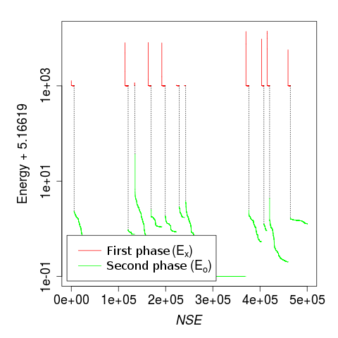
(a) 1BXP

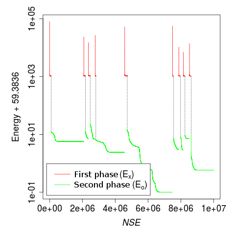
(b) 1AGT

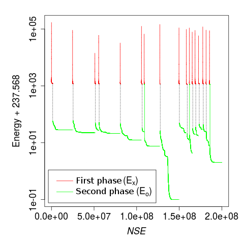
(c) 2EWH

Figure 5: The convergence graphs of the of the best population vector $\vec{x}_{b}^{p}$. Some value was added to the energy because of the logarithmic scale.

In the continuation of the section, we will analyze both optimization phases and the relationship between them. For this purpose, one run was performed for each of the following sequences 1BXP, 1AGT, and 2EWH, with the following stopping conditions $\mathit{NSE}_{\mathit{lmt}}=5\cdot 10^{5}$, $10^{7}$, and $10^{8}$. The convergence graphs of the best population vector $\vec{x}_{b}^{p}$ for all three runs are shown in Fig. 5. The first phase is shown with the red line, while the second phase is shown with the green line. The distance between these two lines is determined by the constant $\lambda$ (see Eq. 4). We can notice that the optimization process is alternated between two optimization phases, the energy value of the first phase is always higher in comparison with the energy value of the second phase, and the optimization process is employed mostly in the second optimization phase. This can also be seen in Table 8. The number of solution evaluations within the first phase $\mathit{NSE}^{1}$ is significantly smaller in comparison with the number of solution evaluations within the second phase $\mathit{NSE}^{2}$. A similar relationship can be observed for runtime. From the shown coefficients, we can see that the first phase used only 11.6% of $\mathit{NSE}$ and only 13% of $t$ for sequence 1BXP. For the longer sequences, these percentages are even smaller. A meticulous reader may notice that parameters $H_{c}$ and $P_{b}$ determine the relationship between optimization phases, and this relationship is contrary to the parameter values. The reason for this is in the local search, which is used only in the second phase. When a good solution is reached, the local search is a good mechanism to further improve it. Therefore, the population best vector has a greater likelihood of improvement and, consequently, the second optimization phase takes more time.

Table 9: Comparison of the DE${}_{\text{2P}}$ algorithm with state-of-the-art algorithms with $N_{r}=30$ and $\mathit{NSE}_{\mathit{lmt}}=M\cdot 10^{4}$. The displayed $L_{2}$ represents the percentage of runs where the second optimization phase is reached. The detailed results are shown in Table 11.

label	$M$	DE${}_{\text{2P}}$		DE${}_{\text{lscr}}$ BoskovicAB18	SGDE Rakhshani19	jDE Brest06 ; BoskovicAB18	L-SHADE Tanabe14 ; BoskovicAB18	BE-ABC Li15 ; Li15f
		$E_{\mathit{mean}}$	$L_{2}$	$E_{\mathit{mean}}$	$E_{\mathit{mean}}$	$E_{\mathit{mean}}$	$E_{\mathit{mean}}$	$E_{\mathit{mean}}$
1CB3	20	7.3586	100.0%	4.5108	6.0772	3.8988	2.7916	5.9417
1BXL	20	15.0934	100.0%	12.5045	14.6894	12.4047	10.5428	11.6942
1EDP	20	12.7113	100.0%	8.1986	9.9649	7.4667	4.5900	8.0500
2H3S	20	15.1167	100.0%	11.5310	12.6380	10.7931	10.3830	10.4618
2KGU	20	38.9910	100.0%	33.6539	38.7383	29.5511	26.6282	22.7195
1TZ4	20	29.8651	100.0%	21.6863	24.1430	16.9135	16.4693	14.9436
1TZ5	20	33.7524	100.0%	25.9996	29.7668	20.3655	20.6403	17.4859
1AGT	20	45.7362	93.3%	39.1897	41.4230	30.7770	29.3564	25.6024
1CRN	20	69.9021	66.7%	62.2668	64.2589	46.9030	46.9604	42.3083
1HVV	20	38.2981	0.0%	35.9335	38.4222	20.9541	25.4910	21.5386
1GK4	20	42.0417	0.0%	42.0261	46.9844	22.3218	32.9082	27.0410
1PCH	80	94.6396	46.7%	87.5748	-	51.7904	59.9509	51.6674
2EWH	80	152.3479	16.7%	162.3482	-	88.8341	104.9692	94.5785
F13	4	4.4955	100.0%	3.0907	-	3.2002	2.7742	2.8196
F21	4	9.4729	96.7%	6.5538	-	6.3647	5.9441	5.2674
F34	12	15.2387	96.7%	13.3057	-	11.5144	10.5170	8.3239
F55	20	25.6430	50.0%	22.4019	-	16.9941	17.1060	14.4556

5.4 Comparison with state-of-the-art algorithms

In this section, our algorithm is compared with state-of-the-art algorithms according to the number of function evaluations and the best obtained energy values.

5.4.1 Number of function evaluations

In the first comparison, the stopping condition was $\mathit{NSE}_{\mathit{lmt}}$, which was set according to the literature BoskovicAB18 ; Li15 . The obtained results are shown in Tables 9 and 11. The best-obtained energy values are marked in bold typeface. It can be observed that DE${}_{\text{2P}}$ obtained the second best $E_{\mathit{mean}}$ for longer sequences 1HVV, 1GK4, and 2EWH, while, for all the remaining sequences, it obtained the best $E_{\mathit{mean}}$. Table 9 additionally shows $L_{2}$, that represents the percentage of runs where the second optimization phase has been reached. From these results, we can see that, for some sequences, DE${}_{\text{2P}}$ cannot reach the second optimization phase in all the runs because the value of $\mathit{NSE}_{\mathit{lmt}}$ is relatively small. Some solvers from the literature cannot perform experiments with a larger value of $\mathit{NSE}_{\mathit{lmt}}$ in a reasonable time because of their runtime complexity. It is also interesting that, although DE${}_{\text{2P}}$ did not reach the second optimization phase in any run for sequences 1HVV and 1GK4, it obtained relatively good results. The SGDE algorithm obtained the best results for these two sequences. Although SGDE is based on the surrogate model, DE${}_{\text{2P}}$ outperformed it on all sequences where the second optimization phase had been reached in most of the runs. For sequence 2EWH, DE${}_{\text{2P}}$ obtained the second phase in only 5 out of 30 runs, and this can be the reason why it obtained the second best $E_{\mathit{mean}}$ and DE${}_{\text{lscr}}$ the best $E_{\mathit{mean}}$. When significantly larger number of solution evaluations was allowed with $t_{\mathit{lmt}}=4$ days, DE${}_{\text{2P}}$ outperformed DE${}_{\text{lscr}}$ significantly on all longer sequences, including sequence 2EWH (see Table 7).

Table 10: Comparisons of the best energy values reported in the literature and the best energy values obtained by DE${}_{\text{2P}}$.

label	L	DE${}_{\text{2P}}$	DE${}_{\text{lscr}}$	SGDE	BE-ABC
			BoskovicAB18	Rakhshani19	Li15 ; Li15f
1BXP	13	5.6104	5.6104	-	2.8930
1CB3	13	8.4589	8.4589	8.3690	8.4580
1BXL	16	17.3962	17.3962	16.4788	15.9261
1EDP	17	15.0092	15.0092	14.2928	13.9276
2ZNF	18	18.3402	18.3402	-	5.8150
1EDN	21	21.4703	21.4703	-	7.6890
2H3S	25	21.1519	21.1519	17.3037	18.3299
1ARE	29	25.2883	25.2800	-	10.2580
2KGU	34	53.6756	52.7165	46.0917	28.1423
1TZ4	37	43.1890	43.0229	31.5031	39.4901
1TZ5	37	50.2703	49.3868	39.0536	45.3233
1AGT	38	66.2973	65.1990	46.2295	51.8019
1CRN	46	95.3159	92.9853	78.2451	54.7253
2KAP	60	89.5013	85.5099	-	27.1400
1HVV	75	101.6018	95.4475	52.5588	47.4484
1GK4	84	112.3674	106.4193	57.9654	49.4871
1PCH	88	166.7194	156.5252	-	91.3508
2EWH	98	257.0741	245.5193	201.0500	146.8231
F13	13	6.9961	6.9961	-	6.9961
F21	21	16.5544	16.5544	-	15.6258
F34	34	31.3732	31.3459	-	28.0516
F55	55	54.9269	52.0558	-	42.5814
F89	89	86.4318	83.5761	-	-

5.4.2 The best energy values

Finally, to demonstrate the superiority of our algorithm in comparison with other algorithms, the best energy values are compared for all selected sequences. This comparison is shown in Table 10. Note that these results were obtained with different experiments. In the case of SGDE, the 30 independent runs were limited with 200,000 solution evaluations. The running environment was Matlab under Windows 7 operating system on an Intel(R) Core i7-6700HQ CPU with 8 GB of RAM. BE-ABC terminated the optimization process when there had been no evolution for up to 5,000,000 consecutive iterations. In this case, a Matlab environment was used on an Intel Core 2 Duo CPU with 2.53 GHz and 2 GB of RAM under Windows XP. DE${}_{\text{2P}}$ and DE${}_{\text{lscr}}$ generated the best solution with the 100 independent runs that were limited with runtime limit ($t_{lmt}$) = 4 days. In this case, the grid environment was used. It was configured to use AMD Opteron 6272 processor with a clock speed of 2.1 GHz, and main memory of 128 GB assigned to 64 cores. The program was implemented in the C++ programming language and the operating system was Linux. We can see that DE${}_{\text{2P}}$ confirms the best energy values for shorter sequences, and the new best-known solutions were obtained for all sequences with 29 or more monomers. The solution vectors obtained by DE${}_{\text{2P}}$ are shown in Tables 12 and 13, while their graphical representation is shown in Fig. 6.

6 Conclusions

In this paper, we presented two-phase optimization that was incorporated into our Differential Evolution algorithm for protein folding optimization. In order to improve the efficiency of the algorithm, the optimization process is divided into two phases. The first phase is responsible for forming solutions with a good hydrophobic core quickly, while the second phase is responsible for locating the best solutions. The hydrophobic core represents a set of positions of the hydrophobic amino acids. Therefore, in the first phase, the auxiliary fitness function is used, that includes expression about the quality of the hydrophobic core.

In our experiment, we used 23 sequences for analyzing the proposed mechanism and our algorithm for protein structure optimization. From the obtained results, we can conclude that the proposed two-phase optimization mechanism improves the efficiency of our algorithm. The required runtime for reaching the best-known energy values on small sequences was reduced from 3.3 to 89.3 times. In addition, two-phase optimization pushed the frontiers on finding the best-known solutions with a success rate of 100% for sequences from 18 to 25 monomers. The solutions of these sequences could be optimal. The success rate greater than one is obtained for sequences up to 37 monomers. For these sequences, solutions are close to optimal, or could be optimal. For other sequences, solutions are almost surely not optimal, and for these sequences, the proposed algorithm reached the new best-known solutions.

The proposed algorithm was also compared with state-of-the-art algorithms for protein folding optimization. Although the used stopping criteria that were taken from the literature did not allow our algorithm to reach the second optimization phase in all the runs, our algorithm outperformed all competitors on small sequences, and it is comparable on longer sequences. With the stopping condition of four days, when a significantly larger number of solution evaluations was allowed, it obtained significantly better energy values for all longer sequences.

In the future work, we will try to implement our algorithm by using full atom and coarse-grained Kmiecik16 representations of protein structure.

References

- (1) Backofen, R., Will, S.: A Constraint-Based Approach to Fast and Exact Structure Prediction in Three-Dimensional Protein Models. Constraints 11(1), 5–30 (2006). doi:10.1007/s10601-006-6848-8
- (2) Bošković, B., Brest, J.: Differential evolution for protein folding optimization based on a three-dimensional AB off-lattice model. Journal of Molecular Modeling 22, 1–15 (2016). doi:10.1007/s00894-016-3104-z
- (3) Bošković, B., Brest, J.: Genetic Algorithm with Advanced Mechanisms Applied to the Protein Structure Prediction in a Hydrophobic-Polar Model and Cubic Lattice. Applied Soft Computing 45, 61–70 (2016). doi:10.1016/j.asoc.2016.04.001
- (4) Bošković, B., Brest, J.: Protein folding optimization using differential evolution extended with local search and component reinitialization. Inf. Sci. 454-455, 178–199 (2018). doi:10.1016/j.ins.2018.04.072
- (5) Brest, J., Greiner, S., Bošković, B., Mernik, M., Žumer, V.: Self-Adapting Control Parameters in Differential Evolution: A Comparative Study on Numerical Benchmark Problems. IEEE Trans. Evol. Comput 10(6), 646–657 (2006). doi:10.1109/TEVC.2006.872133
- (6) Das, S., Mullick, S.S., Suganthan, P.: Recent advances in differential evolution – An updated survey. Swarm and Evolutionary Computation 27, 1–30 (2016). doi:10.1016/j.swevo.2016.01.004
- (7) Das, S., Suganthan, P.N.: Differential Evolution: A Survey of the State-of-the-Art. IEEE Trans. Evol. Comput 15(1), 4–31 (2011). doi:10.1109/TEVC.2010.2059031
- (8) Del Ser, J., Osaba, E., Molina, D., Yang, X.S., Salcedo-Sanz, S., Camacho, D., Das, S., Suganthan, P.N., Coello Coello, C.A., Herrera, F.: Bio-inspired computation: Where we stand and what’s next. Swarm and Evolutionary Computation 48, 220–250 (2019). doi:10.1016/j.swevo.2019.04.008
- (9) Fan, J., Duan, H., Xie, G., Shi, H.: Improved Biogeography-Based Optimization approach to secondary protein prediction. In: 2014 International Joint Conference on Neural Networks (IJCNN), pp. 4223–4228 (2014). doi:10.1109/IJCNN.2014.6889417
- (10) Fister, I., Fister, D., Deb, S., Mlakar, U., Brest, J., Fister, I.: Post hoc analysis of sport performance with differential evolution. Neural Computing and Applications (2018). doi:10.1007/s00521-018-3395-3
- (11) Hart, W.E., Newman, A.: Protein Structure Prediction with Lattice Models (2005)
- (12) Hribar, R., Šilc, J., Papa, G.: Construction of Heuristic for Protein Structure Optimization Using Deep Reinforcement Learning. In: P. Korošec, N. Melab, E.G. Talbi (eds.) Bioinspired Optimization Methods and Their Applications, pp. 151–162. Springer International Publishing (2018). doi:10.1007/978-3-319-91641-5_13
- (13) Huang, W., Liu, J.: Structure optimization in a three-dimensional off-lattice protein model. Biopolymers 82(2), 93–98 (2006). doi:10.1002/bip.20400
- (14) Jana, N.D., Das, S., Sil, J.: A Metaheuristic Approach to Protein Structure Prediction: Algorithms and Insights from Fitness Landscape Analysis. Emergence, Complexity and Computation. Springer International Publishing (2018)
- (15) Jana, N.D., Sil, J., Das, S.: An Improved Harmony Search Algorithm for Protein Structure Prediction Using 3D Off-Lattice Model, pp. 304–314. Springer Singapore, Singapore (2017). doi:10.1007/978-981-10-3728-3_30
- (16) Jana, N.D., Sil, J., Das, S.: Selection of appropriate metaheuristic algorithms for protein structure prediction in AB off-lattice model: a perspective from fitness landscape analysis. Inf. Sci. 391–392, 28–64 (2017). doi:10.1016/j.ins.2017.01.020
- (17) Kalegari, D.H., Lopes, H.S.: An improved parallel differential evolution approach for protein structure prediction using both 2D and 3D off-lattice models. In: 2013 IEEE Symposium on Differential Evolution (SDE), pp. 143–150 (2013). doi:10.1109/SDE.2013.6601454
- (18) Kennedy, D., Norman, C.: Editorial: So much more to know. Science 309, 78–102 (2005). doi:10.1126/science.309.5731.78b
- (19) Kmiecik, S., Gront, D., Kolinski, M., Wieteska, L., Dawid, A.E., Kolinski, A.: Coarse-Grained Protein Models and Their Applications. Chemical Reviews 116(14), 7898–7936 (2016). doi:10.1021/acs.chemrev.6b00163
- (20) Li, B., Chiong, R., Lin, M.: A balance-evolution artificial bee colony algorithm for protein structure optimization based on a three-dimensional AB off-lattice model. Computational Biology and Chemistry 54, 1–12 (2015). doi:10.1016/j.compbiolchem.2014.11.004
- (21) Li, B., Lin, M., Liu, Q., Li, Y., Zhou, C.: Protein folding optimization based on 3D off-lattice model via an improved artificial bee colony algorithm. Journal of Molecular Modeling 21(10), 261 (2015). doi:10.1007/s00894-015-2806-y
- (22) Li, Y., Zhou, C., Zheng, X.: The Application of Artificial Bee Colony Algorithm in Protein Structure Prediction. In: L. Pan, G. Păun, M. Pérez-Jiménez, T. Song (eds.) Bio-Inspired Computing - Theories and Applications, Communications in Computer and Information Science, vol. 472, pp. 255–258. Springer Berlin Heidelberg (2014). doi:10.1007/978-3-662-45049-9_42
- (23) Lin, J., Zhong, Y., Li, E., Lin, X., Zhang, H.: Multi-agent simulated annealing algorithm with parallel adaptive multiple sampling for protein structure prediction in AB off-lattice model. Applied Soft Computing 62, 491–503 (2018). doi:10.1016/j.asoc.2017.09.037
- (24) Lin, X., Zhang, X., Zhou, F.: Protein structure prediction with local adjust tabu search algorithm. BMC Bioinformatics 15(Suppl 15) (2014). doi:10.1186/1471-2105-15-S15-S1
- (25) Mount, D.W.: Bioinformatics: Sequence and Genome Analysis. New York: Cold Spring Harbor Laboratory Press (2001)
- (26) Opara, K.R., Arabas, J.: Differential Evolution: A survey of theoretical analyses. Swarm and Evolutionary Computation 44, 546–558 (2019). doi:10.1016/j.swevo.2018.06.010
- (27) Parpinelli, R.S., Benítez, C.M., Cordeiro, J., Lopes, H.S.: Performance Analysis of Swarm Intelligence Algorithms for the 3D-AB off-lattice Protein Folding Problem. Journal of Multiple-Valued Logic and Soft Computing 22, 267–287 (2014). doi:10.1016/j.engappai.2013.06.010
- (28) Parpinelli, R.S., Lopes, H.S.: An Ecology-Based Evolutionary Algorithm Applied to the 2D-AB Off-Lattice Protein Structure Prediction Problem. In: 2013 Brazilian Conference on Intelligent Systems, pp. 64–69 (2013). doi:10.1109/BRACIS.2013.19
- (29) Petsko, G., Ringe, D.: Protein Structure and Function. Primers in biology. New Science Press (2004)
- (30) Rajasekhar, A., Lynn, N., Das, S., Suganthan, P.: Computing with the collective intelligence of honey bees – A survey. Swarm and Evolutionary Computation 32, 25–48 (2017). doi:10.1016/j.swevo.2016.06.001
- (31) Rakhshani, H., Idoumghar, L., Lepagnot, J., Brévilliers, M.: Speed up differential evolution for computationally expensive protein structure prediction problems. Swarm and Evolutionary Computation (2019). doi:10.1016/j.swevo.2019.01.009
- (32) Rashid, M.A., Iqbal, S., Khatib, F., Hoque, M.T., Sattar, A.: Guided macro-mutation in a graded energy based genetic algorithm for protein structure prediction. Computational Biology and Chemistry 61, 162–177 (2016). doi:10.1016/j.compbiolchem.2016.01.008
- (33) Rashid, M.A., Khatib, F., Hoque, M.T., Sattar, A.: An Enhanced Genetic Algorithm for Ab InitioProtein Structure Prediction. IEEE Transactions on Evolutionary Computation 20(4), 627–644 (2016). doi:10.1109/TEVC.2015.2505317
- (34) Rashid, M.A., Newton, M.A.H., Hoque, M.T., Sattar, A.: Mixing energy models in genetic algorithms for on-lattice protein structure prediction. BioMed Research International 2013 (2013). doi:10.1155/2013/924137
- (35) Sar, E., Acharyya, S.: Genetic algorithm variants in Predicting Protein Structure. In: 2014 International Conference on Communication and Signal Processing, pp. 321–325 (2014). doi:10.1109/ICCSP.2014.6949854
- (36) Singh, H.K., Islam, M.M., Ray, T., Ryan, M.: Nested evolutionary algorithms for computationally expensive bilevel optimization problems: Variants and their systematic analysis. Swarm and Evolutionary Computation 48, 329 – 344 (2019). doi:j.swevo.2019.05.002
- (37) Sinha, A., Malo, P., Deb, K.: A Review on Bilevel Optimization: From Classical to Evolutionary Approaches and Applications. IEEE Transactions on Evolutionary Computation 22(2), 276–295 (2018). doi:10.1109/TEVC.2017.2712906
- (38) Stillinger, F.H., Head-Gordon, T., Hirshfeld, C.L.: Toy model for protein folding. Phys. Rev. E 48, 1469–1477 (1993). doi:10.1103/PhysRevE.48.1469
- (39) Tanabe, R., Fukunaga, A.: Improving the search performance of SHADE using linear population size reduction. In: 2014 IEEE Congress on Evolutionary Computation (CEC2014), pp. 1658–1665. IEEE (2014)
- (40) Wang, Y., Filippini, M., Bacco, G., Bianchi, N.: Parametric design and optimization of magnetic gears with differential evolution method. IEEE Transactions on Industry Applications pp. 1–1 (2019). doi:10.1109/TIA.2019.2901774
- (41) Wang, Y., Guo, G., Chen, L.: Chaotic Artificial Bee Colony algorithm: A new approach to the problem of minimization of energy of the 3D protein structure. Molecular Biology 47(6), 894–900 (2013). doi:10.1134/S0026893313060162
- (42) Wong, K.C., Wu, C.H., Mok, R.K.P., Peng, C., Zhang, Z.: Evolutionary Multimodal Optimization Using the Principle of Locality. Inf. Sci. 194, 138–170 (2012). doi:10.1016/j.ins.2011.12.016
- (43) Zamuda, A., Brest, J.: Vectorized Procedural Models for Animated Trees Reconstruction using Differential Evolution. Inf. Sci. 278, 1–21 (2014)
- (44) Zhou, C., Hou, C., Wei, X., Zhang, Q.: Improved hybrid optimization algorithm for 3D protein structure prediction. Journal of Molecular Modeling 20(7), 2289 (2014). doi:10.1007/s00894-014-2289-2
- (45) Zhou, C., Sun, C., Wang, B., Wang, X.: An improved stochastic fractal search algorithm for 3D protein structure prediction. Journal of Molecular Modeling 24(6), 125 (2018). doi:10.1007/s00894-018-3644-5