Doubly virtual $(\pi^{0},\eta,\eta^{\prime})\to\gamma^{*}\gamma^{*}$ transition form factors in the light-front quark model

Abstract

We report our investigation on the doubly virtual transition form factors (TFFs) $F_{{\rm P}\gamma^{*}}(Q^{2}_{1},Q^{2}_{2})$ for the ${\rm P}\to\gamma^{*}(q_{1})\gamma^{*}(q_{2})\;({\rm P}=\pi^{0},\eta,\eta^{\prime})$ transitions using the light-front quark model (LFQM). Performing a LF calculation in the exactly solvable manifestly covariant Bethe-Salpeter (BS) model as the first illustration, we use the $q^{+}_{1}=0$ frame and find that both LF and manifestly covariant calculations produce exactly the same results for $F_{{\rm P}\gamma^{*}}(Q^{2}_{1},Q^{2}_{2})$. This confirms the absence of the LF zero mode in the doubly virtual TFFs. We then map this covariant BS model to the standard LFQM using the more phenomenologically accessible Gaussian wave function provided by the LFQM analysis of meson mass spectra. For the numerical analyses of $F_{{\rm P}\gamma^{*}}(Q^{2}_{1},Q^{2}_{2})$, we compare our LFQM results with the available experimental data and the perturbative QCD (pQCD) and vector meson dominance (VMD) model predictions. As $(Q^{2}_{1},Q^{2}_{2})\to\infty$, our LFQM result for doubly virtual TFF is consistent with the pQCD prediction, i.e. $F_{{\rm P}\gamma^{*}}(Q^{2}_{1},Q^{2}_{2})\sim 1/(Q^{2}_{1}+Q^{2}_{2})$, while it differs greatly from the result of the VMD model, which behaves as $F^{\rm VMD}_{{\rm P}\gamma^{*}}(Q^{2}_{1},Q^{2}_{2})\sim 1/(Q^{2}_{1}Q^{2}_{2})$. Our LFQM prediction for $F_{\eta^{\prime}\gamma^{*}}(Q^{2}_{1},Q^{2}_{2})$ shows an agreement with the very recent experimental data obtained from the $BABAR$ Collaboration for the ranges of $2<(Q^{2}_{1},Q^{2}_{2})<60$ GeV².

I Introduction

The meson-photon transitions such as ${\rm P}\to\gamma^{(*)}\gamma^{(*)}({\rm P}=\pi^{0},\eta,\eta^{\prime})$ with one or two virtual photons have been of interest to both theoretical and experimental physics communities since they are the simplest possible bound state processes in quantum chromodynamics (QCD) and they play a significant role in allowing both the low- and high-energy precision tests of the standard model.

In particular, both singly virtual and doubly virtual transition form factors (TFFs) are required to estimate the hadronic light-by-light (HLbL) scattering contribution to the muon anomalous magnetic moment $(g-2)_{\mu}$. The HLbL contribution is in principle obtained by integrating some weighting functions times the product of a single-virtual and a double-virtual TFF for spacelike momentum JN ; Ny2016 ; Lattice16 . The single-virtual TFFs have been measured either from the spacelike $e^{+}e^{-}\to e^{+}e^{-}{\rm P}$ process in the single tag mode CELLO91 ; CLEO98 ; BES15_Pi or from the timelike Dalitz decays ${\rm P}\to\bar{\ell}\ell\gamma$ NA60 ; NA60-17 ; A22014 ; A22011 ; A2pi ; BES15 where $(2m_{\ell})^{2}\leq q^{2}\leq m^{2}_{\rm P}$. The timelike region beyond the single Dalitz decays may be accessed through the $e^{+}e^{-}\to{\rm P}\gamma$ annihilation processes, and the $BABAR$ Collaboration BABAR06 measured the timelike $F_{\eta^{(\prime)}\gamma}$ TFFs from the reaction $e^{+}e^{-}\to\eta^{(\prime)}\gamma$ at an average $e^{+}e^{-}$ center of mass energy of $\sqrt{s}=10.58$ GeV.

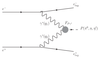
Figure 1: The diagram for the $e^{+}e^{-}\to e^{+}e^{-}{\rm P}$ process.

Very recently, the $BABAR$ Collaboration BABAR18 measured for the first time the double-virtual $\gamma^{*}(q_{1})\gamma^{*}(q_{2})\to\eta^{\prime}$ TFF $F_{\eta^{\prime}\gamma^{*}}(Q^{1}_{1},Q^{2}_{2})$ in the spacelike(i.e. $Q^{2}_{1(2)}=-q^{2}_{1(2)}>0$) kinematic region of $2<Q^{2}_{1},Q^{2}_{2}<60$ GeV² by using the $e^{+}e^{-}\to e^{+}e^{-}\eta^{\prime}$ process in the double-tag mode as shown in Fig. 1. It is very interesting to note that the measurement of $F_{{\rm P}\gamma^{*}}(Q^{1}_{1},Q^{2}_{2})$ at large $Q^{2}_{1}$ and $Q^{2}_{2}$ distinguishes the predictions of the model inspired by perturbative QCD(pQCD) BL80 ; Braaten83 , $F^{pQCD}_{{\rm P}\gamma^{*}}(Q^{2}_{1},Q^{2}_{2})\sim 1/(Q^{2}_{1}+Q^{2}_{2})$, from those of the vector meson dominance (VMD) model VDM1 ; VDM2 ; VDM3 , $F^{VDM}_{{\rm P}\gamma^{*}}(Q^{2}_{1},Q^{2}_{2})\sim 1/(Q^{2}_{1}Q^{2}_{2})$, while both models predict the same asymptotic dependence $F^{asy}_{{\rm P}\gamma}(Q^{2},0)\sim 1/Q^{2}$ as $Q^{2}\to\infty$.

The low-energy behavior of the TFF for the doubly virtual $\pi^{0}\to\gamma^{*}\gamma^{*}$ transition was recently investigated within a Dyson-Schwinger and Bethe-Salpeter (BS) framework Weil . In our previous analysis CRJ17 , we explored the TFF $F_{P\gamma}(Q^{2},0)$ for the single-virtual ${\rm P}\to\gamma^{*}\gamma~{}({\rm P}=\pi^{0},\eta,\eta^{\prime})$ transition both in the spacelike and timelike region using the light-front quark model (LFQM) CJ_99 ; CJ_DA ; PiGam16 ; CJ_PLB ; CJBc . In particular, we presented the new direct method to explore the timelike region without resorting to mere analytic continuation from a spacelike to a timelike region. Our direct calculation in the timelike region has shown the complete agreement with not only the analytic continuation result from the spacelike region but also the result from the dispersion relation between the real and imaginary parts of the form factor.

The purpose of this work is to extend our previous analysis CRJ17 to compute the TFF for the doubly virtual $\eta^{\prime}\to\gamma^{*}\gamma^{*}$ transition and compare with the recent $BABAR$ data for $F_{{\rm P}\gamma^{*}}(Q^{2}_{1},Q^{2}_{2})$ BABAR18 . We also present the TFFs for $(\eta,\pi^{0})\to\gamma^{*}\gamma^{*}$ as well to complete the analysis of doubly virtual photon-pseudoscalar meson transitions in our LFQM.

The paper is organized as follows. In Sec. II, we discuss the TFFs for the doubly virtual ${\rm P}\to\gamma^{*}\gamma^{*}$ transitions in an exactly solvable model first based on the covariant BS model of (3+1)-dimensional fermion field theory to check the existence (or absence) of the LF zero mode Zero1 ; Zero2 ; Zero3 ; Zero4 as one can pin down the zero mode exactly in the manifestly covariant BS model BCJ02 ; BCJ03 ; TWV ; TWPS ; TWPS17 . Performing both the manifestly covariant calculation and the LF calculation, we explicitly show the equivalence between the two results and the absence of the zero-mode contribution to the TFF. The $\eta-\eta^{\prime}$ mixing scheme for the calculations of the $(\eta,\eta^{\prime})\to\gamma^{*}\gamma^{*}$ TFFs is also introduced in this section. In Sec. III, we apply the self-consistent correspondence relations [see, e.g., Eq. (35) in TWPS  ] between the covariant BS model and the LFQM and we present the standard LFQM calculation with the more phenomenologically accessible model wave functions provided by the LFQM analysis of meson mass spectra CJ_PLB ; CJ_99 . In Sec. IV, we present our numerical results for the $(\pi^{0},\eta,\eta^{\prime})\to\gamma^{*}\gamma^{*}$ TFFs and compare them with the available experimental data. Summary and discussion follow in Sec. V.

II Manifestly Covariant Model

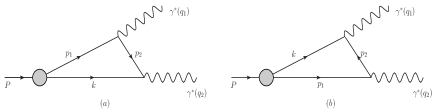
Figure 2: One-loop Feynman diagrams that contribute to ${\rm P}\to\gamma^{*}\gamma^{*}$. (a) and (b) represent the amplitudes of the virtual photon with momentum $q_{1}$ being attached to the quark and antiquark lines.

The TFF $F_{{\rm P}\gamma^{*}}$ for the doubly virtual ${\rm P}(P)\to\gamma^{*}(q_{1})\gamma^{*}(q_{2})$ (${\rm P}=\pi^{0},\eta,\eta^{\prime}$) transition is defined via the amplitude $T$ as follows:

$$T=ie^{2}F_{{\rm P}\gamma^{*}}(q^{2}_{1},q^{2}_{2})\epsilon^{\mu\nu\rho\sigma}\epsilon_{1\mu}\epsilon_{2\nu}q_{1\rho}q_{2\sigma},$$ (1)

where $P$ is the four-momenta of the pseudoscalar meson, $q_{1(2)}$ and $\varepsilon_{1(2)}$ are the momenta and polarization vectors of two virtual photons 1 and 2, respectively. This process is illustrated by the one-loop Feynman diagrams in Figs. 2(a) and 2(b), which represent the amplitudes of the virtual photon with momenta $q_{1}$ being attached to the quark and antiquark lines, respectively. While we shall only discuss the amplitude shown in Fig. 2(a), the total amplitude should of course include the contribution from the process in Fig. 2(b) as well.

In the exactly solvable manifestly covariant BS model, the covariant amplitude $T$ in Fig. 2 (a) is obtained with the following momentum integral:

$$T=ie_{Q}e_{\bar{Q}}N_{c}\int\frac{d^{4}k}{(2\pi)^{4}}\frac{H_{0}}{N_{p_{1}}N_{k}N_{p_{2}}}S,$$ (2)

where $N_{c}$ is the number of colors and $e_{Q}~{}(e_{\bar{Q}})$ is the quark (antiquark) electric charge. The denominators $N_{p_{j}}(=p_{j}^{2}-m_{Q}^{2}+i\epsilon)~{}(j=1,2)$ and $N_{k}(=k^{2}-m_{\bar{Q}}^{2}+i\epsilon)$ come from the intermediate quark and antiquark propagators of mass $m_{Q}=m_{\bar{Q}}$ carrying the internal four-momenta $p_{1}=P-k$, $p_{2}=P-q-k$, and $k$, respectively. The trace term $S$ in Eq. (2) is obtained as

$$S = {\rm Tr}\left[\gamma_{5}\left(/\!\!\!\!\!p_{1}+m_{Q}\right)/\!\!\!\!\!\epsilon_{1}\left(/\!\!\!\!\!p_{2}+m_{Q}\right)/\!\!\!\!\!\epsilon_{2}\left(-/\!\!\!\!k+m_{Q}\right)\right]$$ (3)

$$= 4im_{Q}\epsilon^{\mu\nu\rho\sigma}\epsilon_{1\mu}\epsilon_{2\nu}q_{1\rho}q_{2\sigma}.$$

For the ${\bar{q}}q$ bound-state vertex function $H_{0}=H_{0}(p^{2}_{1},k^{2})$ of the meson, we simply take the constant parameter $g$ in our model calculation. The covariant loop is regularized properly with this constant vertex.

Using the Feynman parametrization for the three propagators $1/(N_{p_{1}}N_{k}N_{p_{2}})$, we obtain the manifestly covariant result by defining the amplitude in Fig. 1(a) as $T_{(a)}=ie_{Q}e_{\bar{Q}}[I^{m_{Q}}_{(a)}]^{\rm Cov}(q^{2}_{1},q^{2}_{2})\epsilon^{\mu\nu\rho\sigma}\epsilon_{1\mu}\epsilon_{2\nu}q_{1\rho}q_{2\sigma}$, where

$$[I^{m_{Q}}_{(a)}]^{\rm Cov} = \frac{N_{c}g}{4\pi^{2}}\int^{1}_{0}dx\int^{1-x}_{0}dy$$ (4)

$$\times\frac{m_{Q}}{(x+y-1)(xM^{2}-yQ^{2}_{2})+xyQ^{2}_{1}+m^{2}_{Q}},$$

with the physical meson mass $M$.

For the LF calculation in parallel with the manifestly covariant one, we use the $q^{+}_{1}=0$ frame, where we take $P=(P^{+},M^{2}/P^{+},0)$; $q_{1}=(0,q^{-}_{1},{\bf q}_{1\perp})$; and $q_{2}=(P^{+},(q^{2}_{2}+{\bf q}^{2}_{1\perp})/P^{+},-{\bf q}_{1\perp})$ so that $q^{2}_{1}=-{\bf q}^{2}_{1\perp}\equiv-Q^{2}_{1}$ and $q^{2}_{2}=-Q^{2}_{2}$.

In this frame, the Cauchy integration of Eq. (2) over $k^{-}$ in Fig. 2(a) yields

$$[I^{m_{Q}}_{(a)}]^{\rm LF}=\frac{N_{c}}{4\pi^{3}}\int^{1}_{0}\frac{dx}{x(1-x)}\int d^{2}{\bf k}_{\perp}\frac{m_{Q}}{Q^{2}_{2}+M^{\prime 2}_{0}}\chi(x,{\bf k}_{\perp}),$$ (5)

where $x$ is the LF longitudinal momentum fraction defined by $k^{+}=(1-x)P^{+}$ and the LF $({\rm P}q\bar{q})$-vertex function

$$\chi(x,{\bf k}_{\perp})=\frac{g}{x(M^{2}-M^{2}_{0})}$$ (6)

is the ordinary LF valence wave function with $M^{2}_{0}=\frac{{\bf k}^{2}_{\perp}+m^{2}_{Q}}{x(1-x)}$ being the invariant mass. Note here that the pole of $N_{k}=0$ is taken for the Cauchy integration to get Eq.(6). The primed momentum variables are defined by $M^{\prime}_{0}=M_{0}({\bf k}_{\perp}\to{\bf k}^{\prime}_{\perp})$ with ${\bf k^{\prime}}_{\perp}={\bf k}_{\perp}+(1-x){\bf q}_{1\perp}$. We confirmed numerically that Eq. (5) exactly coincides with the manifestly covariant result given by Eq. (4). This verifies that the LF result obtained from the $q^{+}_{1}=0$ frame is immune to the LF zero-mode contribution, which could have been the additional contribution right at $p_{1}^{+}=p_{2}^{+}=0$ if it exists. The LF zero mode involves the nonvalence wave function vertex discussed in our previous works CRJ17 ; TWPS . The Lorentz invariance of the TFF is complete in this work without any issue from the LF zero mode.

Since the amplitude of Fig. 2(b) gives the same numerical values as that of Fig. 2(a), we obtain the total result as $I^{m_{Q}}_{\rm tot}=2[I^{m_{Q}}_{(a)}]^{\rm Cov}=2[I^{m_{Q}}_{(a)}]^{\rm LF}$.

III Application of the Light-Front Quark Model

In the standard LFQM CJ_PLB ; CJ_99 ; PiGam16 ; CJ_DA ; CJBc ; Jaus90 ; CCP ; Choi07 approach, the wave function of a ground state pseudoscalar meson as a $q\bar{q}$ bound state is given by

$$\Psi_{\lambda{\bar{\lambda}}}(x,{\bf k}_{\perp})={\phi_{R}(x,{\bf k}_{\perp})\cal R}_{\lambda{\bar{\lambda}}}(x,{\bf k}_{\perp}),$$ (7)

where $\phi_{R}$ is the radial wave function and ${\cal R}_{\lambda{\bar{\lambda}}}$ is the spin-orbit wave function with the helicity $\lambda~{}({\bar{\lambda}})$ of a quark (antiquark).

For the equal quark and antiquark mass $m_{Q}=m_{\bar{Q}}$, the Gaussian wave function $\phi_{R}$ is given by

$$\phi_{R}(x,{\bf k}_{\perp})=\frac{4\pi^{3/4}}{\beta^{3/2}}\sqrt{\frac{M_{0}}{4x(1-x)}}e^{m^{2}_{Q}/2\beta^{2}}e^{-M^{2}_{0}/8\beta^{2}},$$ (8)

where $\partial k_{z}/\partial x=M_{0}/4x(1-x)$ is the Jacobian of the variable transformation $\{x,{\bf k}_{\perp}\}\to{\vec{k}}=({\bf k}_{\perp},k_{z})$ and $\beta$ is the variational parameter fixed by our previous analysis of meson mass spectra CJ_PLB ; CJ_99 ; CJBc . The covariant form of the spin-orbit wave function ${\cal R}_{\lambda{\bar{\lambda}}}$ is given by

$${\cal R}_{\lambda{\bar{\lambda}}}=\frac{\bar{u}_{\lambda}(p_{Q})\gamma_{5}v_{{\bar{\lambda}}}(p_{\bar{Q}})}{\sqrt{2}M_{0}},$$ (9)

and it satisfies $\sum_{\lambda{\bar{\lambda}}}{\cal R}_{\lambda{\bar{\lambda}}}^{\dagger}{\cal R}_{\lambda{\bar{\lambda}}}=1$. Thus, the normalization of our wave function is given by

$$\int^{1}_{0}dx\int\frac{d^{2}{\bf k}_{\perp}}{16\pi^{3}}|\phi_{R}(x,{\bf k}_{\perp})|^{2}=1.$$ (10)

In our previous analysis of the twist-2 and twist-3 DAs of pseudoscalar and vector mesons TWV ; TWPS ; TWPS17 and the pion electromagnetic form factor TWPS , we have shown that standard LF (SLF) results of the LFQM are obtained by the replacement of the LF vertex function $\chi$ in the BS model with the Gaussian wave function $\phi_{R}$ as follows [see, e.g., Eq. (35) in TWPS ]

$$\sqrt{2N_{c}}\frac{\chi(x,{\bf k}_{\perp})}{1-x}\to\frac{\phi_{R}(x,{\bf k}_{\perp})}{\sqrt{{\bf k}^{2}_{\perp}+m_{Q}^{2}}},\;M\to M_{0},$$ (11)

where $M\to M_{0}$ implies that the physical mass $M$ included in the integrand of BS amplitude (except $M$ in the vertex function $\chi$) has to be replaced with the invariant mass $M_{0}$ since the SLF results of the LFQM are obtained from the requirement of all constituents being on their respective mass shell. The correspondence in Eq. (11) is valid again in this analysis of a ${\rm P}\to\gamma^{*}\gamma^{*}$ transition.

Applying the correspondence given by Eq. (11) to $[I^{m_{Q}}_{(a)}]^{\rm LF}$ in Eq. (5) and including the contribution from Fig. 2(b) as well, we obtain the full result of $[I^{m_{Q}}_{\rm tot}]^{\rm LFQM}\equiv I^{m_{Q}}_{\rm QM}$ in our LFQM as follows:

$$I^{m_{Q}}_{\rm QM}=\frac{\sqrt{2N_{c}}}{4\pi^{3}}\int^{1}_{0}\frac{dx}{x}\int d^{2}{\bf k}_{\perp}\frac{m_{Q}}{(Q^{2}_{2}+M^{\prime 2}_{0})}\frac{\phi_{R}(x,{\bf k}_{\perp})}{\sqrt{{\bf k}^{2}_{\perp}+m^{2}_{Q}}}.$$ (12)

For $(\eta,\eta^{\prime})\to\gamma^{*}\gamma^{*}$ transitions, making use of the $\eta-\eta^{\prime}$ mixing scheme, the flavor assignment of $\eta$ and $\eta^{\prime}$ mesons in the quark-flavor basis $\eta_{q}=(u\bar{u}+d\bar{d})/\sqrt{2}$ and $\eta_{s}=s\bar{s}$ is given by FKS

$$\left(\begin{array}[]{cc}\eta\\ \eta^{\prime}\end{array}\,\right)=\left(\begin{array}[]{cc}\cos\phi\;\;-\sin\phi\\ \sin\phi\;\;\;\;\;\cos\phi\end{array}\,\right)\left(\begin{array}[]{c}\eta_{q}\\ \eta_{s}\end{array}\,\right).$$ (13)

Using this mixing scheme and including the electric charge factors, we obtain the transition form factors $F_{{\rm P}\gamma^{*}}(Q^{2}_{1},Q^{2}_{2})$ for ${\rm P}\to\gamma^{*}\gamma^{*}~{}({\rm P}=\pi^{0},\eta,\eta^{\prime})$ transitions as follows

$$F_{\pi\gamma^{*}}(Q^{2}_{1},Q^{2}_{2}) = \frac{(e^{2}_{u}-e^{2}_{d})}{\sqrt{2}}I^{m_{u(d)}}_{\rm QM},$$

$$F_{\eta\gamma^{*}}(Q^{2}_{1},Q^{2}_{2}) = \cos\phi\;\frac{(e^{2}_{u}+e^{2}_{d})}{\sqrt{2}}I^{m_{u(d)}}_{\rm QM}-\sin\phi\;e^{2}_{s}I^{m_{s}}_{\rm QM},$$

$$F_{\eta^{\prime}\gamma^{*}}(Q^{2}_{1},Q^{2}_{2}) = \sin\phi\;\frac{(e^{2}_{u}+e^{2}_{d})}{\sqrt{2}}I^{m_{u(d)}}_{\rm QM}+\cos\phi\;e^{2}_{s}I^{m_{s}}_{\rm QM}.$$ (14)

While the quadratic (linear) Gell-Mann-Okubo mass formula prefers $\phi\simeq 44.7^{\circ}$ ($\phi\simeq 31.7^{\circ}$) PDG18 , the KLOE Collaboration KLOE extracted the pseudoscalar mixing angle $\phi$ by measuring the ratio ${\rm BR}(\phi\to\eta^{\prime}\gamma)/{\rm BR}(\phi\to\eta\gamma)$. The measured values are $\phi=(39.7\pm 0.7)^{\circ}$ and $(41.5\pm 0.3_{\rm stat}\pm 0.7_{\rm syst}\pm 0.6_{\rm th})^{\circ}$ with and without the gluonium content for $\eta^{\prime}$, respectively. In this work, however, we use $\phi=37^{\circ}\pm 5^{\circ}$ to check the sensitivity of our LFQM.

For a sufficiently high spacelike momentum transfer $(Q^{2}_{1},Q^{2}_{2})$ region, our LFQM result for $F_{\pi\gamma^{*}}(Q^{2}_{1},Q^{2}_{2})$ can be approximated in the leading order (LO) as follows:

$$F^{\rm LO}_{\pi\gamma^{*}}(Q^{2}_{1},Q^{2}_{2})\simeq C_{\pi}\int^{1}_{0}dx\;\frac{\phi_{2;\pi}(x)}{(1-x)Q^{2}_{1}+xQ^{2}_{2}},$$ (15)

where $C_{\pi}=(\sqrt{2}/3)f_{\pi}$, with $f_{\pi}$ the pseudoscalar meson decay constant and $\phi_{2;\pi}(x)$ is the twist-2 pion distribution amplitude (DA) in our LFQM given by TWV ; TWPS ; TWPS17

$$\phi_{2;\pi}(x) = \frac{\sqrt{2N_{c}}}{f_{\pi}8\pi^{3}}\int d^{2}{\bf k}_{\perp}\frac{\phi_{R}(x,{\bf k}_{\perp})}{\sqrt{{\bf k}^{2}_{\perp}+m_{Q}^{2}}}{m_{Q}}.$$ (16)

Our result for $\phi_{2;\pi}(x)$ can be found in Ref. CJ_DA . As one can see from Eq. (15), while the singly virtual TFF $F_{\pi\gamma^{*}}(Q^{2},0)$ above some intermediate values of momentum transfer is known to be quite sensitive to the shape of DA, the doubly virtual TFF is not sensitive to the shape of DA since the amplitude $T_{H}=1/((1-x)Q^{2}_{1}+xQ^{2}_{2})$ is finite at the end points of $x$, i.e. $x=0,1$.

We note that the pQCD LO result for $F_{\pi\gamma^{*}}(Q^{2}_{1},Q^{2}_{2})$ can be obtained from replacing $\phi_{2;\pi}(x)$ in Eq. (15) with the asymptotic form $\phi^{asy}_{2;\pi}(x)=6x(1-x)$ BL80 . Taking the same asymptotic form $6x(1-x)$ for the quark DAs, the pQCD LO results for $(\eta,\eta^{\prime})$ TFFs can also be obtained by replacing the factor $C_{\pi}$ in Eq. (15) with $C_{\eta}=(5\sqrt{2}/9)f_{\eta_{q}}\cos\phi-(2/9)f_{\eta_{s}}\sin\phi$ for $F_{\eta\gamma^{*}}(Q^{2}_{1},Q^{2}_{2})$ and with $C_{\eta^{\prime}}=(5\sqrt{2}/9)f_{\eta_{q}}\sin\phi+(2/9)f_{\eta_{s}}\cos\phi$ for $F_{\eta^{\prime}\gamma^{*}}(Q^{2}_{1},Q^{2}_{2})$, where $f_{\eta_{q}}$ and $f_{\eta_{s}}$ are the weak decay constants for the $|\eta_{q}\rangle$ and $|\eta_{s}\rangle$ states, respectively. For this transition to two highly off-shell photons, the pQCD expression for the next-to-leading order (NLO) component can be found in Ref. Braaten83 .

IV Numerical Results

Table 1: The constituent quark masses $m_{Q}(Q=u(d),s)$ (in GeV) and the Gaussian parameters $\beta_{Q{\bar{Q}}}$ (in GeV) for the linear confining potentials obtained from the variational principle in our LFQM CJ_PLB ; CJ_99 ; CJ_DA .

$m_{u(d)}$	$m_{s}$	$\beta_{Q{\bar{Q}}}$	$\beta_{s{\bar{s}}}$
0.22	0.45	0.3659	0.4128

In our numerical calculations within the standard LFQM, we use the model parameters (i.e. constituent quark masses $m_{Q}$ and Gaussian parameters $\beta_{Q{\bar{Q}}}$) for the linear confining potentials given in Table 1, which were obtained from the calculation of meson mass spectra using the variational principle in our LFQM CJ_PLB ; CJ_99 ; CJ_DA . The analysis for singly virtual TFFs $F_{{\rm P}\gamma}(Q^{2},0)$ can be found in our previous work CRJ17 .

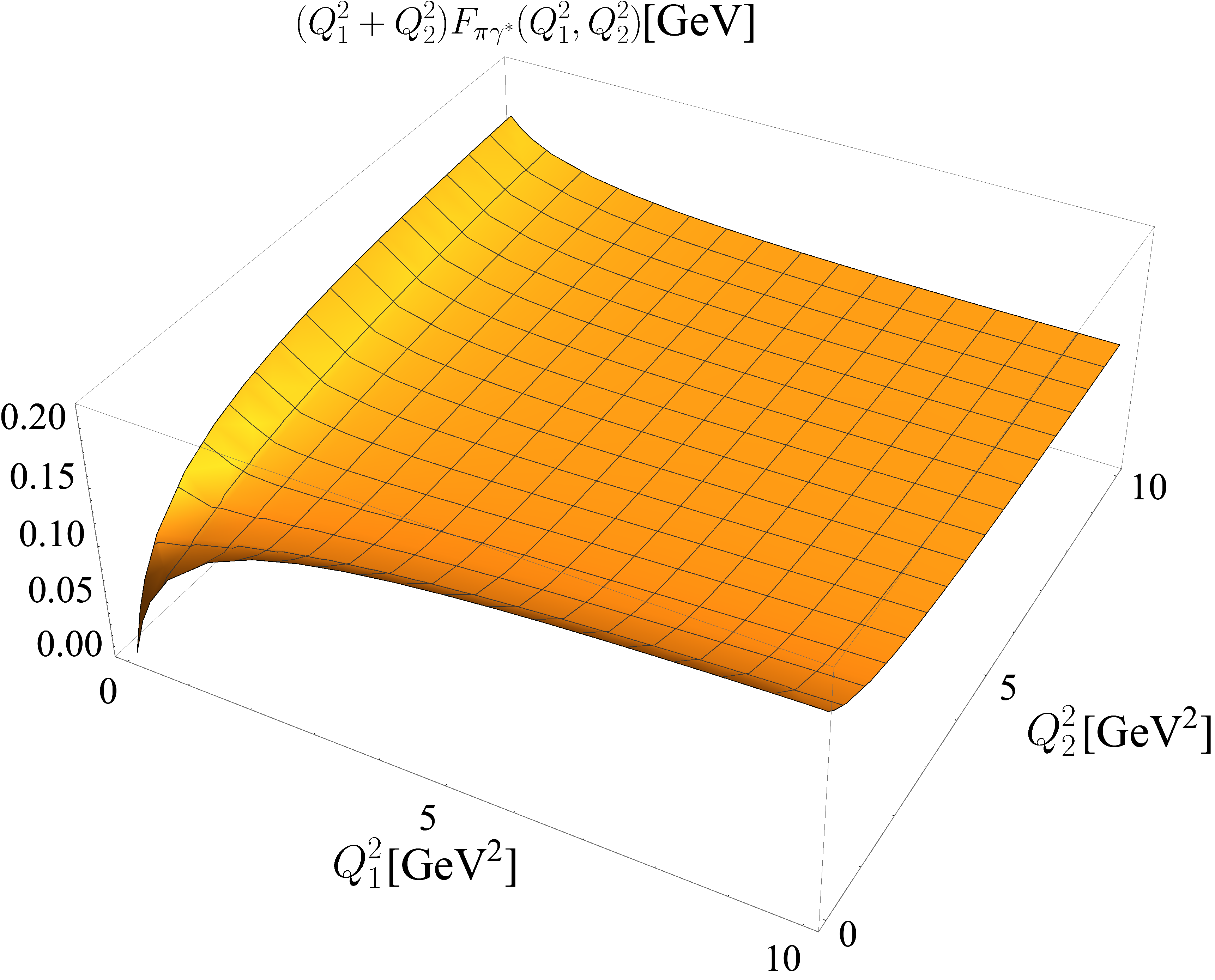
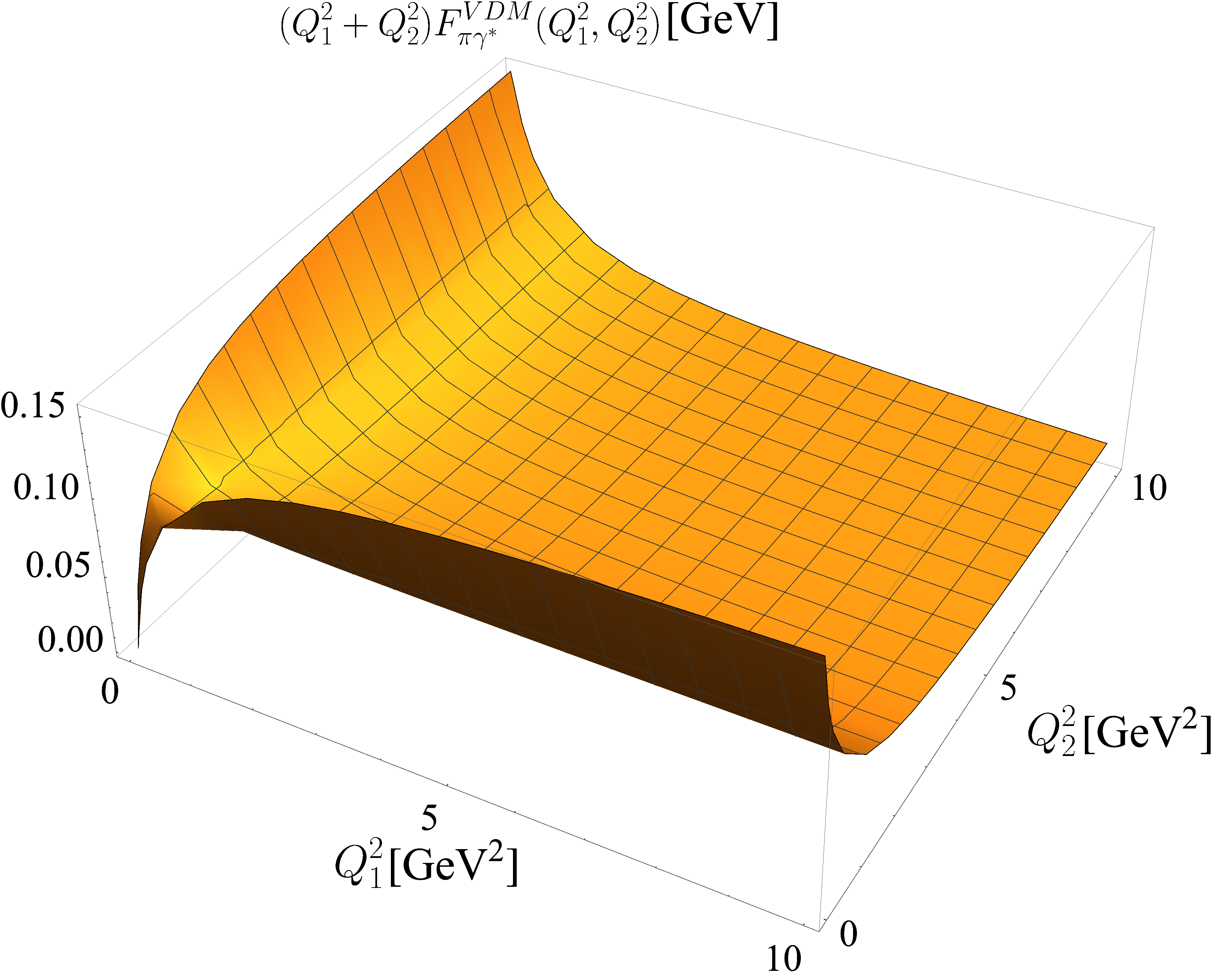
Figure 3: The three-dimensional plots for $(Q^{2}_{1}+Q^{2}_{2})F_{\pi\gamma^{*}}(Q^{2}_{1},Q^{2}_{2})$ obtained from Eq. (III) (upper panel) compared with the VMD result (lower panel) for the range of $0<(Q^{2}_{1},Q^{2}_{2})<10$ GeV².

In Fig. 3, we show the three-dimensional plots for $(Q^{2}_{1}+Q^{2}_{2})F_{\pi\gamma^{*}}(Q^{2}_{1},Q^{2}_{2})$ for the $0<(Q^{2}_{1},Q^{2}_{2})<10$ GeV² range obtained from Eq. (III) and compare our LFQM result (upper panel) with the result from the VMD model (lower panel), which is given by BABAR18

$$F^{\rm VMD}_{{\rm P}\gamma^{*}}(Q^{2}_{1},Q^{2}_{2})=\frac{F_{{\rm P}\gamma}(0,0)}{(1+Q^{2}_{1}/\Lambda^{2}_{\rm P})(1+Q^{2}_{2}/\Lambda^{2}_{\rm P})},$$ (17)

where we take $\Lambda_{\rm P}=775$ MeV corresponding to the $\rho$-pole and the central value of the experimental data PDG18 , $F^{\rm Exp.}_{\pi\gamma}(0,0)=0.272(3)$ GeV^-1 for $F_{\pi\gamma}(0,0)$. As we discussed before, while our LFQM result for doubly virtual TFF behaves as $F_{\pi\gamma^{*}}(Q^{2}_{1},Q^{2}_{2})\sim 1/(Q^{2}_{1}+Q^{2}_{2})$ as $(Q^{2}_{1},Q^{2}_{2})\to\infty$, which is consistent with the pQCD prediction, the result of the VMD model behaves as $F^{\rm VMD}_{\pi\gamma^{*}}(Q^{2}_{1},Q^{2}_{2})\sim 1/(Q^{2}_{1}Q^{2}_{2})$. On the other hand, for the singly virtual TFF such as $F_{\pi\gamma^{*}}(Q^{2}_{1}=Q^{2},0)$ or $F_{\pi\gamma^{*}}(0,Q^{2}_{2}=Q^{2})$, the two models show the same scaling behavior $Q^{2}F_{\pi\gamma^{*}}(Q^{2},0)\to{\rm constant}$. One can also see from Fig. 3 that our LFQM result for the TFF is in general larger in the asymmetric limit (e.g., $Q^{2}_{1}=Q^{2},Q^{2}_{2}=0$) than in the symmetric limit (i.e., $Q^{2}_{1}=Q^{2}_{2}$), which persists up to an asymptotically large momentum transfer region. The same observation was made in Ref. Weil .

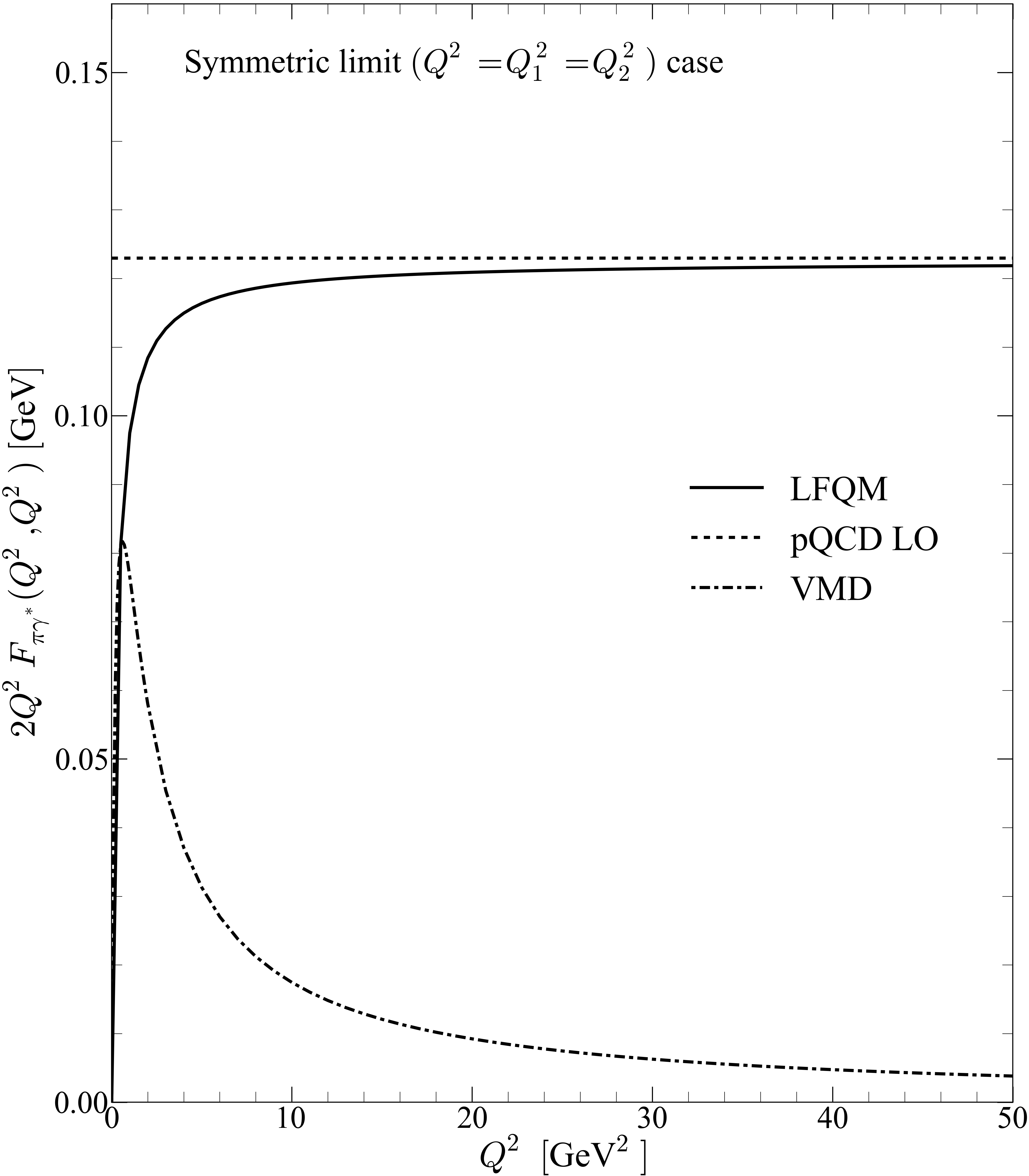
Figure 4: The two-dimensional plot for $2Q^{2}F_{\pi\gamma^{*}}(Q^{2},Q^{2})$ in the symmetric limit ($Q^{2}=Q^{2}_{1}=Q^{2}_{2})$ for the $0<Q^{2}<50$ GeV² region compared with the pQCD LO and the VMD model predictions.

In Fig. 4, we show the two-dimensional plot for $2Q^{2}F_{\pi\gamma^{*}}(Q^{2},Q^{2})$ in the symmetric limit ($Q^{2}=Q^{2}_{1}=Q^{2}_{2})$ for the $0<Q^{2}<50$ GeV² region compared with the pQCD LO and the VMD model predictions. In this symmetric limit case, the different behavior of $Q^{2}F_{\pi\gamma^{*}}(Q^{2},Q^{2})$ between our LFQM result (solid line) $Q^{2}F_{\pi\gamma^{*}}(Q^{2},Q^{2})\to{\rm constant}$ and the VMD result (dotted-dashed line) $Q^{2}F_{\pi\gamma^{*}}(Q^{2},Q^{2})\to 1/Q^{2}$ can be clearly seen as $Q^{2}\to\infty$. Comparing our LFQM result and the pQCD LO (dashed line) prediction, while the NLO contribution is still greater than 10$\%$ for the $Q^{2}\leq 2$ GeV² region, the NLO contribution becomes less than 5$\%$ for the $Q^{2}\geq 6$ GeV² region.

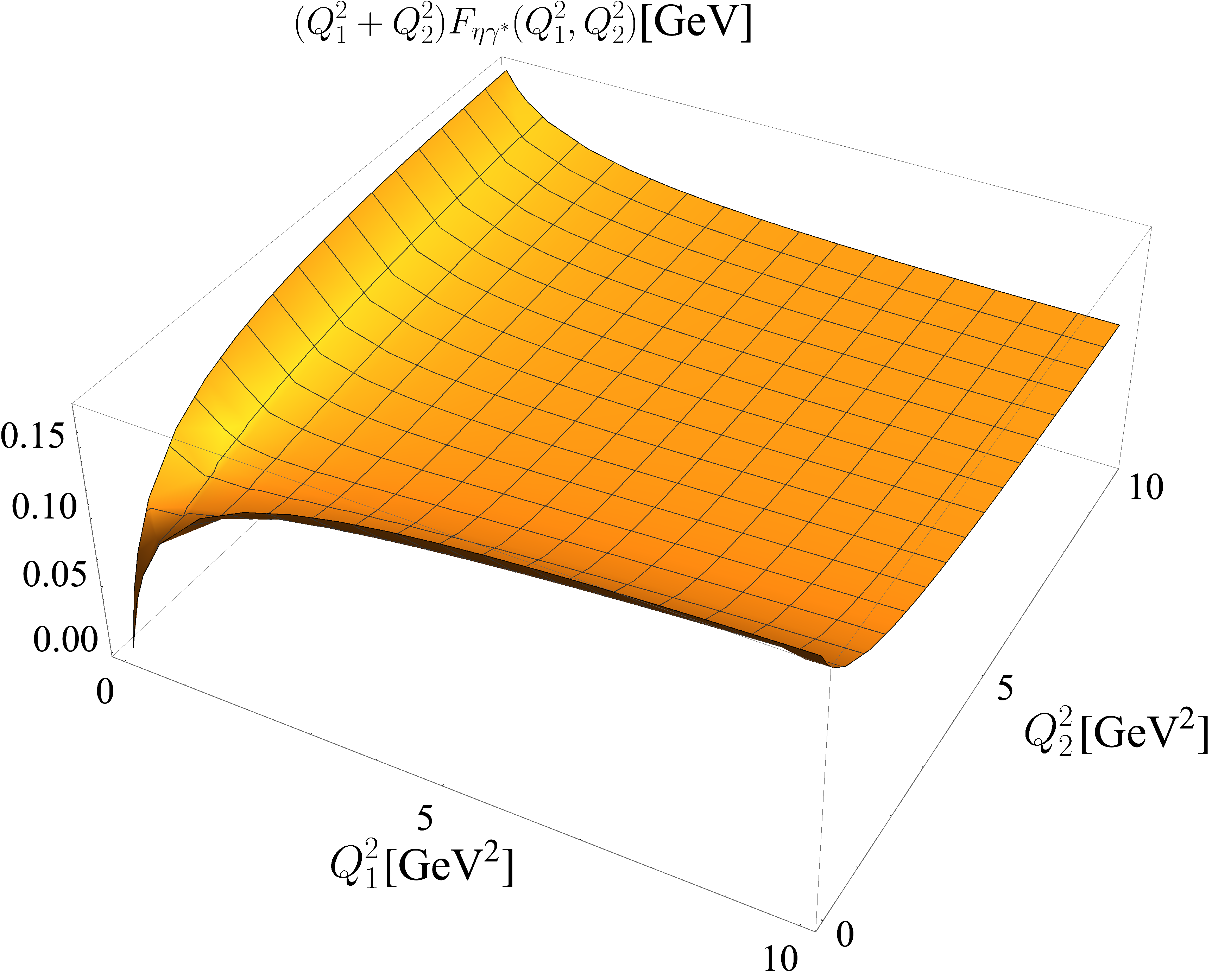
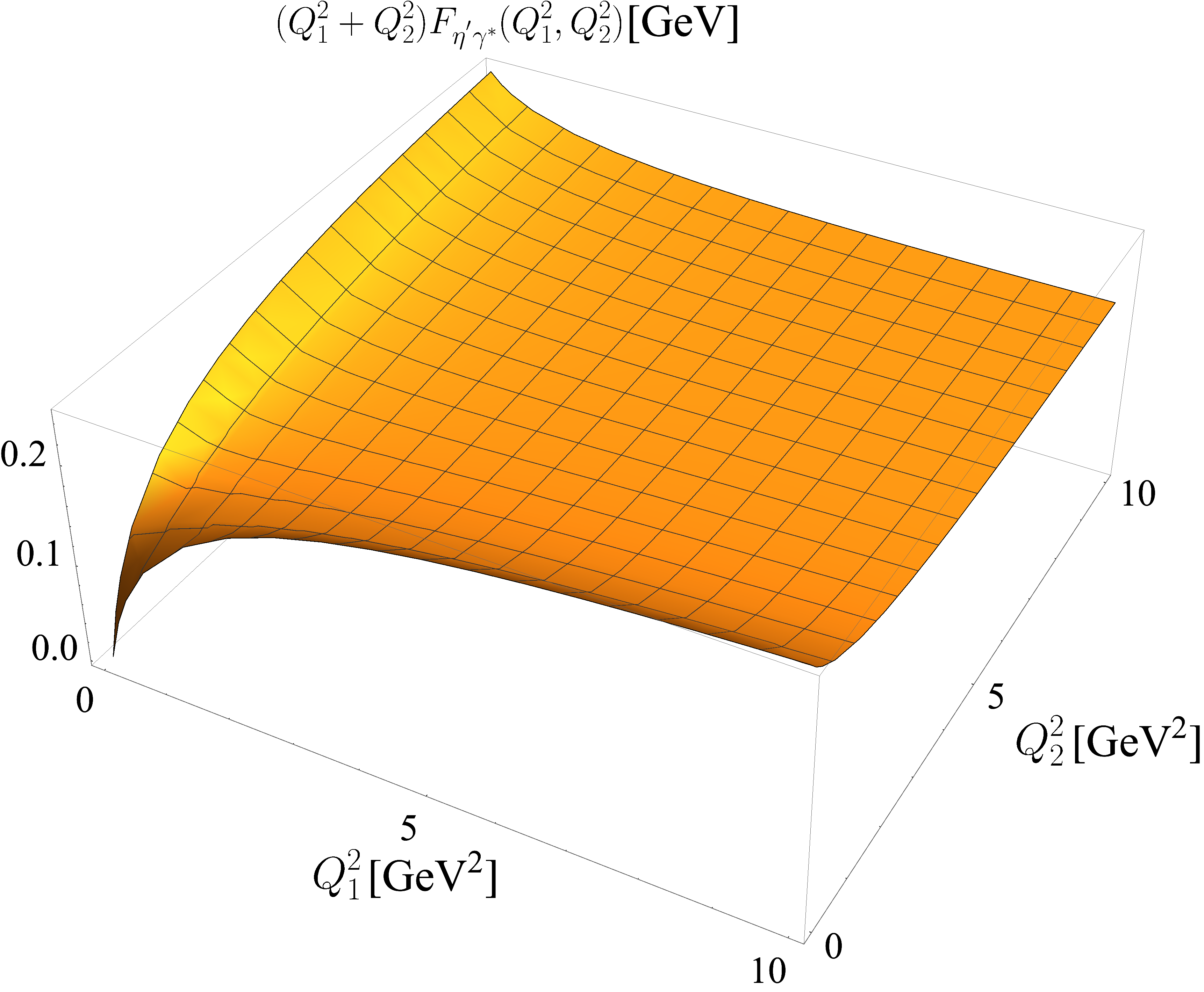
Figure 5: The three-dimensional plots for $(Q^{2}_{1}+Q^{2}_{2})F_{\eta\gamma^{*}}(Q^{2}_{1},Q^{2}_{2})$ (upper panel) and $(Q^{2}_{1}+Q^{2}_{2})F_{\eta^{\prime}\gamma^{*}}(Q^{2}_{1},Q^{2}_{2})$ (lower panel) obtained from Eq. (III) with $\phi=37^{\circ}$ for the range of $0<(Q^{2}_{1},Q^{2}_{2})<10$ GeV².

In Fig. 5, we show the three-dimensional plots for $(Q^{2}_{1}+Q^{2}_{2})F_{\eta\gamma^{*}}(Q^{2}_{1},Q^{2}_{2})$ (upper panel) and $(Q^{2}_{1}+Q^{2}_{2})F_{\eta^{\prime}\gamma^{*}}(Q^{2}_{1},Q^{2}_{2})$ (lower panel) obtained from Eq. (III) with $\phi=37^{\circ}$ for the range of $0<(Q^{2}_{1},Q^{2}_{2})<10$ GeV². As one can see from Figs. 3 and 4, all three TFFs $F_{(\pi,\eta,\eta^{\prime})\gamma^{*}}(Q^{2}_{1},Q^{2}_{2})$ obtained from our LFQM show the same scaling behavior as the pQCD predicted.

Table 2: The transition form factors $F_{(\pi,\eta,\eta^{\prime})\gamma^{*}}(Q^{2}_{1},Q^{2}_{2})$ (in units of $10^{3}$ GeV^-1) for some ($Q^{2}_{1},Q^{2}_{2}$) values (in units of GeV²) compared with the experimental data BABAR18 for $F^{\rm Exp.}_{\eta^{\prime}\gamma^{*}}$.

$(Q^{2}_{1},Q^{2}_{2})$	$F_{\pi\gamma^{*}}$	$F_{\eta\gamma^{*}}$	$F_{\eta^{\prime}\gamma^{*}}$	$F^{\rm Exp.}_{\eta^{\prime}\gamma^{*}}$
(6.48,6.48)	9.08	$8.48^{+1.18}_{-1.24}$	$13.91^{+0.69}_{-0.79}$	$14.32^{+1.95}_{-1.89}\pm 0.83\pm 0.14$
(16.85,16.85)	3.58	$3.29^{+0.47}_{-0.50}$	$5.55^{+0.27}_{-0.31}$	$5.35^{+1.71}_{-2.15}\pm 0.31\pm 0.42$
(14.83,4.27)	6.76	$6.33^{+0.87}_{-0.92}$	$10.32^{+0.51}_{-0.59}$	$8.24^{+1.16}_{-1.13}\pm 0.48\pm 0.65$
(38.11,14.95)	2.40	$2.21^{+0.32}_{-0.33}$	$3.71^{+0.18}_{-0.21}$	$6.07^{+1.09}_{-1.07}\pm 0.35\pm 1.21$
(45.63,45.63)	1.33	$1.22^{+0.18}_{-0.19}$	$2.08^{+0.10}_{-0.11}$	$8.71^{+3.96}_{-4.02}\pm 0.50\pm 1.04$

In Table 2, we summarize our LFQM results for the transition form factors $F_{(\pi,\eta,\eta^{\prime})\gamma^{*}}(Q^{2}_{1},Q^{2}_{2})$ (in units of $10^{3}$ GeV^-1) for some ($Q^{2}_{1},Q^{2}_{2}$) values (in units of GeV²) compared with the experimental data BABAR18 for $F^{\rm Exp.}_{\eta^{\prime}\gamma^{*}}$ with the statistical, systematic, and model uncertainties. We note that the error estimates for $F_{(\eta,\eta^{\prime})\gamma^{*}}(Q^{2}_{1},Q^{2}_{2})$ in our LFQM results come from the choice of $\eta-\eta^{\prime}$ mixing angle $\phi=(37\pm 5)^{\circ}$. We note for $F_{\eta^{\prime}\gamma^{*}}(Q^{2}_{1},Q^{2}_{2})$ that our LFQM result and the experimental data are compatible with each other and the agreement between the two appears fairly reasonable within a rather large uncertainty of data.

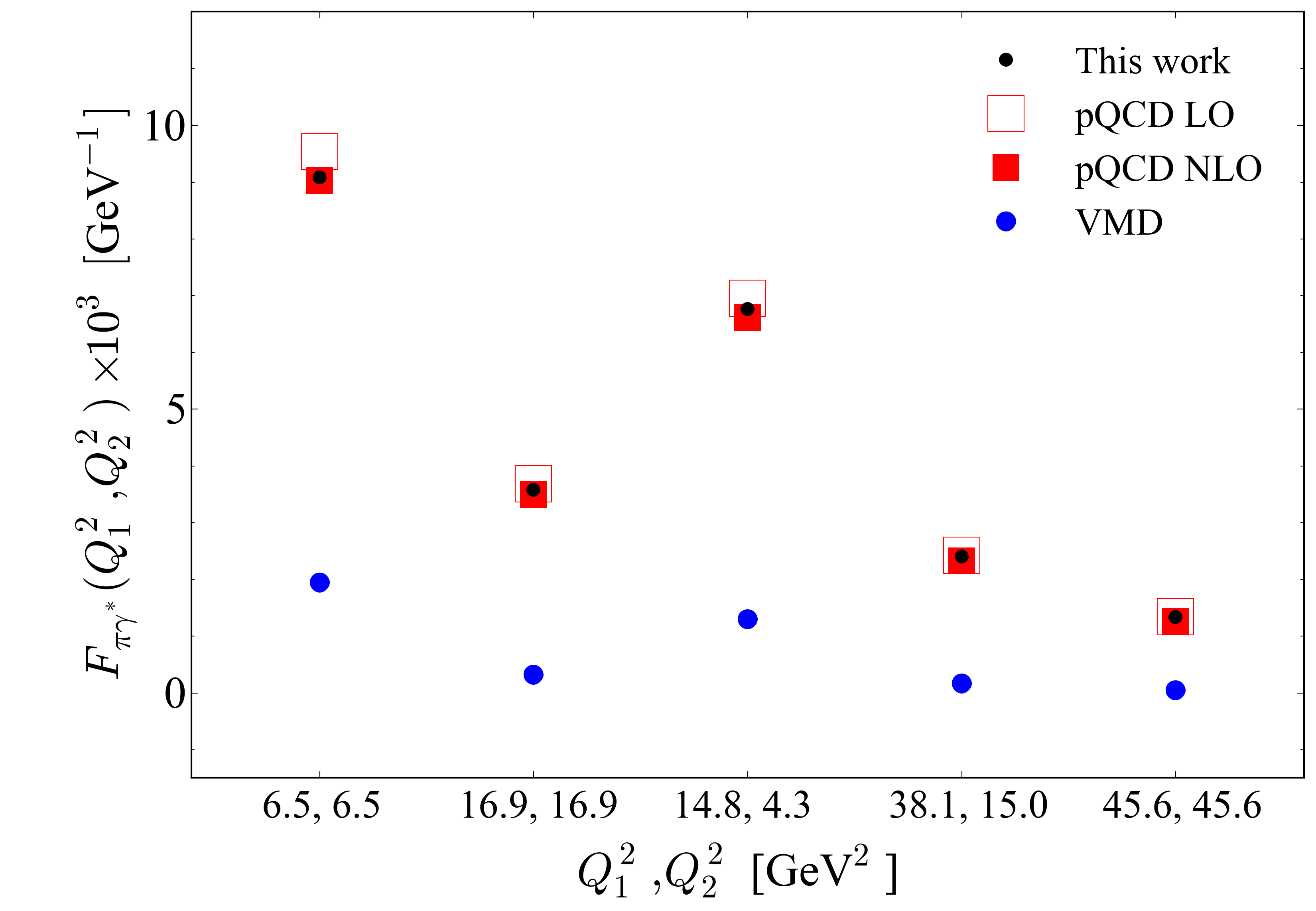
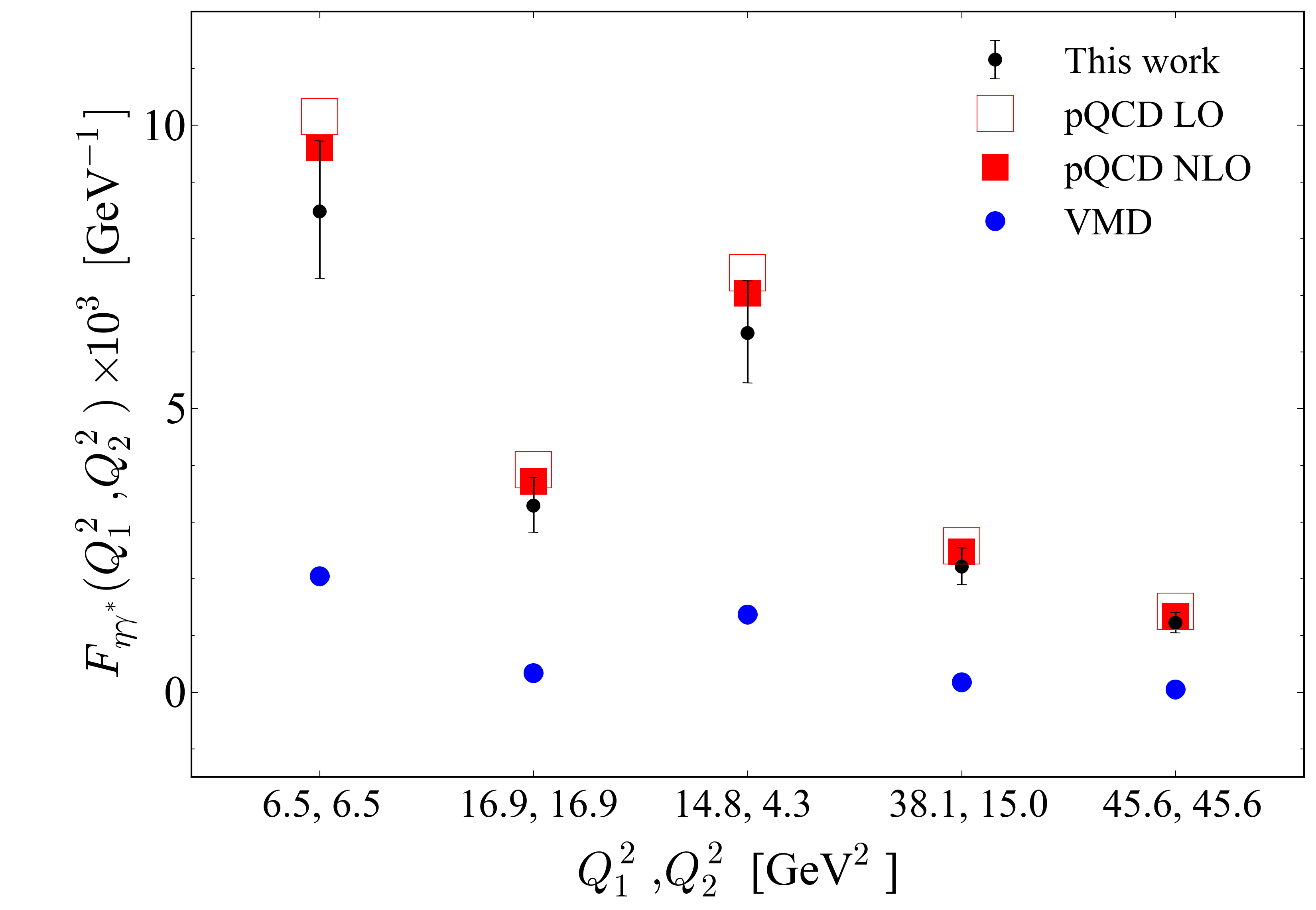
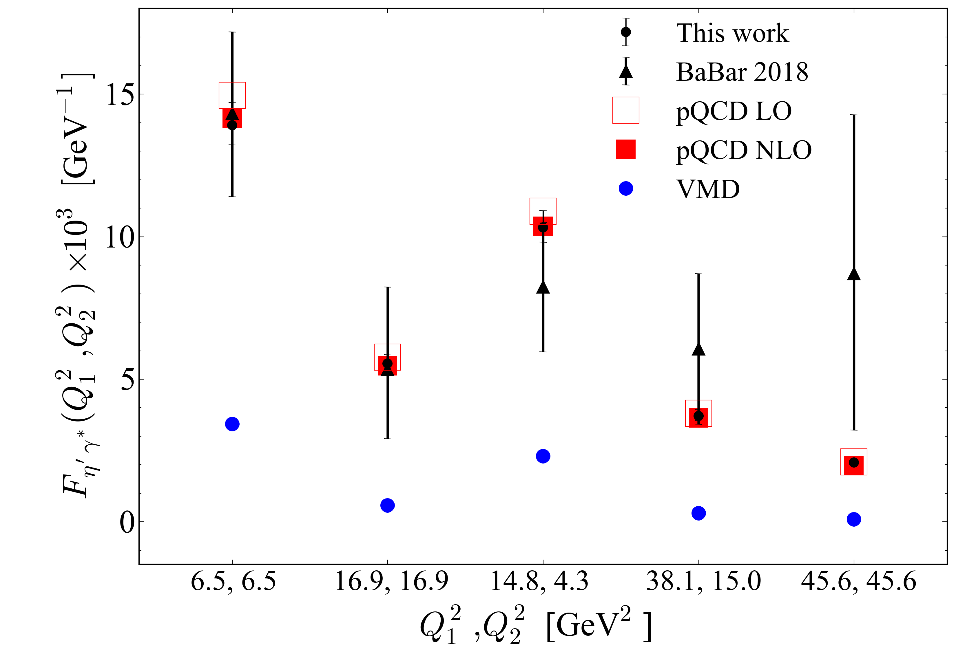
Figure 6: Our LFQM results for $F_{(\pi,\eta,\eta^{\prime})\gamma^{*}}(Q^{2}_{1},Q^{2}_{2})$ (black circles) compared with the pQCD LO (open squares) and NLO(filled squares) predictions; the VMD predictions (blue circles); and the experimental data BABAR18  (triangles, with error bars including the statistical, systematic, and model uncertainties).

In Fig. 6, we show our LFQM results for $F_{(\pi,\eta,\eta^{\prime})\gamma^{*}}(Q^{2}_{1},Q^{2}_{2})$ (black circles) compared with the pQCD LO (open squares) and NLO(filled squares) predictions Braaten83 , VMD predictions (blue circles), and the experimental data BABAR18 (triangles) for $F_{\eta^{\prime}\gamma^{*}}(Q^{2}_{1},Q^{2}_{2})$. We note that the error bars for $F^{\rm Exp.}_{\eta^{\prime}\gamma^{*}}(Q^{2}_{1},Q^{2}_{2})$ include the statistical, systematic, and model uncertainties. As one can see from Fig. 5, our LFQM results for $F_{(\pi,\eta,\eta^{\prime})\gamma^{*}}(Q^{2}_{1},Q^{2}_{2})$ show the same behavior as the pQCD predictions. However, our LFQM predictions are quite different from the VMD model predictions since the two models have different power behaviors of $(Q^{2}_{1},Q^{2}_{2})$ as we discussed before. While the data for $F_{\eta^{\prime}\gamma^{*}}(Q^{2}_{1},Q^{2}_{2})$ measured from $BABAR$ BABAR18 agree with the pQCD and our LFQM predictions, they show a clear disagreement with the VMD model predictions.

V Summary and Discussion

We presented the doubly virtual TFFs $F_{{\rm P}\gamma^{*}}(Q^{2}_{1},Q^{2}_{2})$ for the ${\rm P}\to\gamma^{*}\gamma^{*}\;({\rm P}=\pi^{0},\eta,\eta^{\prime})$ transitions in the standard LF (SLF) approach within the phenomenologically accessible realistic LFQM CJ_PLB ; CJ_99 ; PiGam16 ; CJ_DA ; CJBc . Performing a LF calculation in the covariant BS model as the first illustration, we used the $q^{+}_{1}=0$ frame with $q^{2}_{1}=-{\bf q}^{2}_{1\perp}=-Q^{2}_{1}$, and we found that both LF and manifestly covariant calculations produced exactly the same results for $F_{{\rm P}\gamma^{*}}(Q^{2}_{1},Q^{2}_{2})$. This assured the absence of the LF zero mode in the doubly virtual TFFs as expected CRJ17 .

We then mapped the exactly solvable manifestly covariant BS model to the standard LFQM following the same correspondence relation given by Eq. (11) between the two models that we found in our previous analysis of two-point and three-point functions for the pseudoscalar and vector mesons TWV ; TWPS . This allowed us to apply the more phenomenologically accessible Gaussian wave function provided by the LFQM analysis of meson mass spectra CJ_PLB ; CJ_99 ; PiGam16 ; CJ_DA ; CJBc to the analysis of the doubly virtual $F_{{\rm P}\gamma^{*}}(Q^{2}_{1},Q^{2}_{2})$. For the $(\eta,\eta^{\prime})\to\gamma^{*}\gamma^{*}$ transitions, we used the $\eta-\eta^{\prime}$ mixing angle $\phi$ in the quark-flavor basis varying the $\phi$ values in the range of $\phi=(37\pm 5)^{\circ}$ to check the sensitivity of our LFQM.

For the numerical analyses of $F_{{\rm P}\gamma^{*}}(Q^{2}_{1},Q^{2}_{2})$, we compared our LFQM results with the available experimental data and the other theoretical model predictions such as the pQCD Braaten83 and VMD results. While our LFQM result for the doubly virtual TFF behaves as $F_{{\rm P}\gamma^{*}}(Q^{2}_{1},Q^{2}_{2})\sim 1/(Q^{2}_{1}+Q^{2}_{2})$ as $(Q^{2}_{1},Q^{2}_{2})\to\infty$, which is consistent with the pQCD prediction, the result of the VMD model behaves as $F^{\rm VMD}_{{\rm P}\gamma^{*}}(Q^{2}_{1},Q^{2}_{2})\sim 1/(Q^{2}_{1}Q^{2}_{2})$. Our LFQM prediction for $F_{\eta^{\prime}\gamma^{*}}(Q^{2}_{1},Q^{2}_{2})$ showed a reasonable agreement with the very recent experimental data obtained from the $BABAR$ collaboration for the ranges of $2<(Q^{2}_{1},Q^{2}_{2})<60$ GeV².

References

(1) F. Jegerlehner and A. Nyffeler, Phys. Rep. 477, 1 (2009).
(2) A. Nyffeler, Phys. Rev. D 94, 053006 (2016).
(3) A. Gérardin, H. Meyer, and A. Nyffeler,
Phys. Rev. D 94, 074507 (2016).
(4) H.-J. Behrend et al. (CELLO Collaboration),
Z. Phys. C 49, 401 (1991).
(5) J. Gronberg et al. (CLEO Collaboration),
Phys. Rev. D 57, 33 (1998).
(6) A. Denig (BESIII Collaboration), Nucl. Part. Phys. Proc. 260, 79 (2015).
(7) R. Arnaldi et al. (NA60 Collaboration),
Phys. Lett. B 677, 260 (2009).
(8) C. Lazzeroni et al. (NA62 Collaboration),
Phys. Lett. B 768, 38 (2017).
(9) P. Aguar-Bartomomé et al. (A2 Collaboration),
Phys. Rev. C 89, 044608 (2014).
(10) H. Berghäuser et al. (A2 Collabortation),
Phys. Lett. B 701, 562 (2011).
(11) P. Adlarson et al. (A2 Collaboration), Phys. Rev. C 95, 025202 (2017).
(12) M. Ablikim et al. (BESIII Collaboration), Phys. Rev. D 92, 012001 (2015).
(13) B. Aubert et al. ( Collaboration), Phys. Rev. D 74, 012002 (2006).
(14) J. P. Lees et al. ( Collaboration), Phys. Rev. D 98, 112002 (2018).
(15) G.P. Lepage and S.J. Brodsky, Phys. Rev. D 22, 2157 (1980).
(16) E. Braaten, Phys. Rev. D 28, 524 (1983).
(17) B.-I. Young, Phys. Rev. 161, 1620 (1967).
(18) L. G. Landsberg, Phys. Rep. 128, 301 (1985).
(19) A. Dorokhov, M. Ivanov, and S. Kovalenko, Phys. Lett. B 677, 145 (2009).
(20) E. Weil, G. Eichmann, C. S. Fischer, and R. Williams, Phys. Rev. D 96, 014021 (2017).
(21) H.-M. Choi, H. -Y. Ryu, and C.-R. Ji, Phys. Rev. D 96, 056008 (2017).
(22) H.-M. Choi and C.-R. Ji, Phys. Rev. D 59, 074015 (1999).
(23) H.-M. Choi and C.-R. Ji, Phys. Rev. D 75, 034019 (2007).
(24) H.-M. Choi and C.-R. Ji, Few-Body Syst. 57, 497 (2016).
(25) H.-M. Choi and C.-R. Ji, Phys. Lett. B 460, 461 (1999).
(26) H.-M. Choi and C.-R. Ji, Phys. Rev. D 80, 054016 (2009).
(27) M. Burkardt, Phys. Rev. D 47, 4628 (1993).
(28) S. J. Brodsky and D. S. Hwang, Nucl. Phys. B 543, 239 (1999).
(29) J.P.B.C. de Melo, J.H.O. Sales, T. Frederico, and P.U. Sauer, Nucl. Phys. A 631, 574c (1998).
(30) H.-M. Choi and C.-R. Ji, Phys. Rev. D 58, 071901(R) (1998).
(31) B.L.G. Bakker, H.-M. Choi, and C.-R. Ji, Phys. Rev. D 65, 116001 (2002).
(32) B.L.G. Bakker, H.-M. Choi, and C.-R. Ji, Phys. Rev. D 67, 113007 (2003).
(33) H.-M. Choi and C.-R. Ji,
Phys. Rev. D 89, 033011 (2014).
(34) H.-M. Choi and C.-R. Ji,
Phys. Rev. D 91, 014018 (2015).
(35) H.-M. Choi and C.-R. Ji,
Phys. Rev. D 95, 056002 (2017); Few-Body Syst. 58, 31 (2017).
(36) T. Feldmann, P. Kroll, and B. Stech,
Phys. Rev. D 58, 114006 (1998).
(37) W. Jaus, Phys. Rev. D 41, 3394 (1990).
(38) P. L. Chung, F. Coester, and W. N. Polyzou,
Phys. Lett. B 205, 545 (1988).
(39) H.-M. Choi, Phys. Rev. D 75, 073016 (2007).
(40) M. Tanabashi et al. (Particle Data Group),
Phys. Rev. D 98, 030001 (2018).
(41) F. Ambrosino et al. (KLOE Collaboration),
Phys. Lett. B 648, 267 (2007).