Data Amplification: Instance-Optimal Property Estimation

The best-known and most commonly used distribution-property estimation technique uses a plug-in estimator, with empirical frequency replacing the underlying distribution. We present novel linear-time-computable estimators that significantly “amplify” the effective amount of data available. For a large variety of distribution properties including four of the most popular ones and for every underlying distribution, they achieve the accuracy that the empirical-frequency plug-in estimators would attain using a logarithmic-factor more samples.

Specifically, for Shannon entropy and a very broad class of properties including $\ell_{1}$-distance, the new estimators use $n$ samples to achieve the accuracy attained by the empirical estimators with $n\log n$ samples. For support-size and coverage, the new estimators use $n$ samples to achieve the performance of empirical frequency with sample size $n$ times the logarithm of the property value. Significantly strengthening the traditional min-max formulation, these results hold not only for the worst distributions, but for each and every underlying distribution. Furthermore, the logarithmic amplification factors are optimal. Experiments on a wide variety of distributions show that the new estimators outperform the previous state-of-the-art estimators designed for each specific property.

1 Introduction

Recent years have seen significant interest in estimating properties of discrete distributions over large domains [1, 2, 3, 4, 5, 6]. Chief among these properties are support size and coverage, Shannon entropy, and $\ell_{1}$-distance to a known distribution. The main achievement of these papers is essentially estimating several properties of distributions with alphabet size $k$ using just $k/\log k$ samples.

In practice however, the underlying distributions are often simple, and their properties can be accurately estimated with significantly fewer than $k/\log k$ samples. For example, if the distribution is concentrated on a small part of the domain, or is exponential, very few samples may suffice to estimate the property. To address this discrepancy,  [7] took the following competitive approach.

The best-known distribution property estimator is the empirical estimator that replaces the unknown underlying distribution by the observed empirical distribution. For example, with $n$ samples, it estimates entropy by $\sum_{i}(N_{i}/n)\log(n/N_{i})$ where $N_{i}$ is the number of times symbol $i$ appeared. Besides its simple and intuitive form, the empirical estimator is also consistent, stable, and universal. It is therefore the most commonly used property estimator for data-science applications.

The estimator derived in [7] uses $n$ samples and for any underlying distribution achieves the same performance that the empirical estimator would achieve with $n\sqrt{\log n}$ samples. It therefore provides an effective way to amplify the amount of data available by a factor of $\sqrt{\log n}$, regardless of the domain or structure of the underlying distribution.

In this paper we present novel estimators that increase the amplification factor for all sufficiently smooth properties including those mentioned above from $\sqrt{\log n}$ to the information-theoretic bound of $\log n$. Namely, for every distribution their expected estimation error with $n$ samples is that of the empirical estimator with $n\log n$ samples and no further uniform amplification is possible.

It can further be shown [1, 2, 3, 6] that the empirical estimator estimates all of the above four properties with linearly many samples, hence the sample size required by the new estimators is always at most the $k/\log k$ guaranteed by the state-of-the-art estimators.

The current formulation has several additional advantages over previous approaches.

Fewer assumptions

It eliminates the need for some commonly used assumptions. For example, support size cannot be estimated with any number of samples, as arbitrarily-many low-probabilities may be missed. Hence previous research [5, 3] unrealistically assumed prior knowledge of the alphabet size $k$, and additionally that all positive probabilities exceed $1/k$. By contrast, the current formulation does not need these assumptions. Intuitively, if a symbol’s probability is so small that it won’t be detected even with $n\log n$ samples, we do not need to worry about it.

Refined bounds

For some properties, our results are more refined than previously shown. For example, existing results estimate the support size to within $\pm\epsilon k$, rendering the estimates rather inaccurate when the true support size $S$ is much smaller than $k$. By contrast, the new estimation errors are bounded by $\pm\epsilon S$, and are therefore accurate regardless of the support size. A similar improvement holds for support coverage.

Graceful degradation

For the previous results to work, one needs at least $k/\log k$ samples. With fewer samples, the estimators have no guarantees. By contrast, the guarantees of the new estimators work for any sample size $n$. If $n<k/\log k$, the performance may degrade, but will still track that of the empirical estimators with a factor $\log n$ more samples.

Instance optimality

With the recent exception of [7], all modern property-estimation research took a min-max-related approach, evaluating the estimation improvement based on the worst possible distribution for the property. In reality, practical distributions are rarely the worst possible and often quite simple, rendering min-max approach overly pessimistic, and its estimators, typically suboptimal in practice. In fact, for this very reason, practical distribution estimators do not use min-max based approaches [8]. By contrast, our competitive, or instance-optimal, approach provably ensures amplification for every underlying distribution, regardless of its complexity.

In addition, the proposed estimators run in time linear in the sample size, and the constants involved are very small, properties shared by some, though not all existing estimators.

We formalize the foregoing discussion in the following definitions.

Let $\Delta_{k}$ denote the collection of discrete distributions over $[k]:=\{1,\ldots,k\}$. A distribution property is a mapping $F:\Delta_{k}\to\mathbb{R}$. It is additive if it can be written as

$$F(\vec{p}):=\sum_{i\in[k]}f_{i}(p_{i}),$$

where $f_{i}:[0,1]\to\mathbb{R}$ are real functions. Many important distribution properties are additive:

Shannon entropy

$H(\vec{p}):=\sum_{i\in[k]}-p_{i}\log p_{i}$, is the principal measure of information [9], and arises in a variety of machine-learning [10, 11, 12], neuroscience [13, 14, 15], and other applications.

$\boldsymbol{\ell_{1}}$-distance

$D_{\vec{q}}(\vec{p}):=\sum_{i\in[k]}|p_{i}-q_{i}|$, where $\vec{q}$ is a given distribution, is one of the most basic and well-studied properties in the field of distribution property testing [16, 17, 18, 19].

Support size

$S(\vec{p}):=\sum_{i\in[k]}\mathds{1}_{p_{i}>0}$, is a fundamental quantity for discrete distributions, and plays an important role in vocabulary size [20, 21, 22] and population estimation [23, 24].

Support coverage

$C(\vec{p}):=\sum_{i\in[k]}(1-(1-p_{i})^{m})$, for a given $m$, represents the number of distinct elements we would expect to see in $m$ independent samples, arises in many ecological [25, 26, 27, 28], biological [29, 30], genomic [31] as well as database [32] studies.

Given an additive property $F$ and sample access to an unknown distribution $\vec{p}$, we would like to estimate the value of $F(\vec{p})$ as accurately as possible. Let $[k]^{n}$ denote the collection of all length-$n$ sequences, an estimator is a function $\hat{F}:[k]^{n}\to\mathbb{R}$ that maps a sample sequence $X^{n}\sim\vec{p}$ to a property estimate $\hat{F}(X^{n})$. We evaluate the performance of $\hat{F}$ in estimating $F(\vec{p})$ via its mean absolute error (MAE),

$$L(\hat{F},\vec{p},n):=\operatorname*{\mathbb{E}}_{X^{n}\sim\vec{p}}\left|\hat{F}(X^{n})-F(\vec{p})\right|.$$

Since we do not know $\vec{p}$, the common approach is to consider the worst-case MAE of $\hat{F}$ over $\Delta_{k}$,

$$L(\hat{F},n):=\max_{\vec{p}\in\Delta_{k}}L(\hat{F},\vec{p},n).$$

The best-known and most commonly-used property estimator is the empirical plug-in estimator. Upon observing $X^{n}$, let $N_{i}$ denote the number of times symbol $i\in[k]$ appears in $X^{n}$. The empirical estimator estimates $F(\vec{p})$ by

$$\hat{F}^{E}(X^{n}):=\sum_{i\in[k]}f_{i}\left(\frac{N_{i}}{n}\right).$$

Starting with Shannon entropy, it has been shown [2] that for $n\geq k$, the worst-case MAE of the empirical estimator $\hat{H}^{E}$ is

$$L(\hat{H}^{E},n)=\Theta\left({\frac{k}{n}}+\frac{\log k}{\sqrt{n}}\right).$$ (1)

On the other hand, [1, 2, 3, 6] showed that for $n\geq k/{\log k}$, more sophisticated estimators achieve the best min-max performance of

$$L(n):=\min_{\hat{F}}\max_{\vec{p}\in\Delta_{k}}L(\hat{F},\vec{p},n)=\Theta\left(\frac{k}{n\log n}+\frac{\log k}{\sqrt{n}}\right).$$ (2)

Hence up to constant factors, for the “worst” distributions, the MAE of these estimators with $n$ samples equals that of the empirical estimator with $n\log n$ samples. A similar relation holds for the other three properties we consider.

However, the min-max formulation is pessimistic as it evaluates the estimator’s performance based on its MAE for the worst distributions. In many practical applications, the underlying distribution is fairly simple and does not attain this worst-case loss, rather, a much smaller MAE can be achieved. Several recent works have therefore gone beyond worst-case analysis and designed algorithms that perform well for all distributions, not just those with the worst performance [33, 34].

For property estimation, [7] designed an estimator $\hat{F}^{A}$ that for any underlying distribution uses $n$ samples to achieve the performance of the $n\sqrt{\log n}$-sample empirical estimator, hence effectively multiplying the data size by a $\sqrt{\log n}$ amplification factor.

Lemma 1.

[7] For every property $F$ in a large class that includes the four properties above, there is an absolute constant $c_{F}$ such that for all distribution $\vec{p}$ and all $\varepsilon\leq 1$,

$$L(\hat{F}^{A},\vec{p},n)\leq L\left(\hat{F}^{E},\vec{p},\varepsilon n\sqrt{\log n}\right)+c_{F}\cdot\varepsilon.$$

In this work, we fully strengthen the above result and establish the limits of data amplification for all sufficiently smooth additive properties including four of the most important ones. Using Shannon entropy as an example, we achieve a $\log n$ amplification factor. Equations (1) and (2) imply that the improvement over the empirical estimator cannot always exceed $\mathcal{O}(\log n)$, hence up to a constant, this amplification factor is information-theoretically optimal. Similar optimality arguments hold for our results on the other three properties.

Specifically, we derive linear-time-computable estimators $\hat{H}$, $\hat{D}$, $\hat{S}$, $\hat{C}$, and $\hat{F}$ for Shannon entropy, $\ell_{1}$-distance, support size, support coverage, and a broad class of additive properties which we refer to as “Lipschitz properties”. These estimators take a single parameter $\varepsilon$, and given samples $X^{n}$, amplify the data as described below.

Let $a\land b:=\min\{a,b\}$ and abbreviate the support size $S({\vec{p}})$ by $S_{\vec{p}}$. For some absolute constant $c$, the following five theorems hold for all $\varepsilon\leq 1$, all distributions $\vec{p}$, and all $n\geq 1$.

Theorem 1 (Shannon entropy).

$$L(\hat{H},\vec{p},n)\leq L\left(\hat{H}^{E},\vec{p},{\varepsilon n\log n}\right)+c\cdot\left(\varepsilon\land\left(\frac{S_{\vec{p}}}{n}+\frac{1}{n^{0.49}}\right)\right).$$

Note that the estimator does not need to know $S_{\vec{p}}$ or $k$. When $\varepsilon=1$, the estimator amplifies the data by a factor of $\log n$. As $\varepsilon$ decreases, the amplification factor decreases, and so does the extra additive inaccuracy. One can also set $\varepsilon$ to be a vanishing function of $n$, e.g., $\varepsilon=1/\log\log n$. This result may be interpreted as follows. For distributions with large support sizes such that the min-max estimators provide no or only very weak guarantees, our estimator with $n$ samples always tracks the performance of the $n\log n$-sample empirical estimator. On the other hand, for distributions with relatively small support sizes, our estimator achieves a near-optimal $\mathcal{O}(S_{\vec{p}}/n)$-error rate.

In addition, the above result together with Proposition 1 in [35] trivially implies that

Corollary 1.

In the large alphabet regime where $n=o(k/\log k)$, the min-max MAE of estimating Shannon entropy satisfies

$$L(n)\leq(1+o(1))\log\left(1+\frac{k-1}{n\log n}\right).$$

Similarly, for $\ell_{1}$-distance,

Theorem 2 ($\ell_{1}$-distance).

For any $\vec{q}$, we can construct an estimator $\hat{D}$ for $D_{\vec{q}}$ such that

$$L(\hat{D},\vec{p},n)\leq L\left(\hat{D}^{E},\vec{p},\varepsilon^{2}{n\log n}\right)+c\cdot\left(\varepsilon\land\left(\sqrt{\frac{S_{\vec{p}}}{n}}+\frac{1}{n^{0.49}}\right)\right).$$

Besides having an interpretation similar to Theorem 1, the above result shows that for each $\vec{q}$ and each $\vec{p}$, we can use just $n$ samples to achieve the performance of the $n\log n$-sample empirical estimator. More generally, for any additive property $F(\vec{p})=\sum_{i\in[k]}f_{i}(p_{i})$ that satisfies the simple condition: $f_{i}$ is $\mathcal{O}(1)$-Lipschitz, for all $i$,

Theorem 3 (General additive properties).

Given $F$, we can construct an estimator $\hat{F}$ such that

$$L(\hat{F},\vec{p},n)\leq L\left(\hat{F}^{E},\vec{p},\varepsilon^{2}{n\log n}\right)+\mathcal{O}\left(\varepsilon\land\left(\sqrt{\frac{S_{\vec{p}}}{n}}+\frac{1}{n^{0.49}}\right)\right).$$

We refer to the above general distribution property class as the class of “Lipschitz properties”. Note that the $\ell_{1}$-distance $D_{\vec{q}}$, for any $\vec{q}$, clearly belongs to this class.

Lipschitz properties are essentially bounded by absolute constants and Shannon entropy grows at most logarithmically in the support size, and we were able to approximate all with just an additive error. Support size and support coverage can grow linearly in $k$ and $m$, and can be approximated only multiplicatively. We therefore evaluate the estimator’s normalized performance.

Note that for both properties, the amplification factor is logarithmic in the property value, which can be arbitrarily larger than the sample size $n$. The following two theorems hold for $\epsilon\leq e^{-2}$,

Theorem 4 (Support size).

$$\frac{1}{S_{\vec{p}}}L(\hat{S},\vec{p},n)\leq\frac{1}{S_{\vec{p}}}L\left(\hat{S}^{E},\vec{p},|\log^{-2}{\varepsilon}|\cdot n\log S_{\vec{p}}\right)+{c}\left(S_{\vec{p}}^{|\log^{-1}{\varepsilon}|-\frac{1}{2}}+\varepsilon\right).$$

To make the slack term vanish, one can simply set $\varepsilon$ to be a vanishing function of $n$ (or $S_{\vec{p}}$), e.g., $\varepsilon=1/\log n$. Note that in this case, the slack term modifies the multiplicative error in estimating $S_{\vec{p}}$ by only $o(1)$, which is negligible in most applications. Similarly, for support coverage,

Theorem 5 (Support coverage).

Abbreviating $C({\vec{p}})$ by $C_{\vec{p}}$,

$$\frac{1}{C_{\vec{p}}}L(\hat{C},\vec{p},n)\leq\frac{1}{C_{\vec{p}}}L\left(\hat{C}^{E},\vec{p},|\log^{-2}{\varepsilon}|\cdot n\log C_{\vec{p}}\right)+c\left(C_{\vec{p}}^{|\log^{-1}{\varepsilon}|-\frac{1}{2}}+\varepsilon\right).$$

For notational convenience, let $h(p):=-p\log p$ for entropy, $\ell_{q}(p):=|p-q|-q$ for $\ell_{1}$-distance, $s(p):=\mathds{1}_{p>0}$ for support size, and $c(p):=1-(1-p)^{m}$ for support coverage. In the next section, we provide an outline of the remaining contents, and a high-level overview of our techniques.

2 Outline and technique overview

In the main paper, we focus on Shannon entropy and prove a weaker version of Theorem 1.

Theorem 6.

For all $\varepsilon\leq 1$ and all distributions $\vec{p}$, the estimator $\hat{H}$ described in Section 5 satisfies

$$L(\hat{H},\vec{p},n)\leq L(\hat{H}^{E},\vec{p},\varepsilon n\log n)+\left(1+c\cdot\varepsilon\right)\land\left(\frac{S_{\vec{p}}}{\varepsilon n}+\frac{1}{n^{0.49}}\right).$$

The proof of Theorem 6 in the rest of the paper is organized as follows. In Section 3, we present a few useful concentration inequalities for Poisson and binomial random variables. In Section 4, we relate the bias of the $n$-sample empirical estimator to the degree-$n$ Bernstein polynomial $B_{n}(h,x)$ by $B_{n}(h,p_{i})=\mathbb{E}[h(N_{i}/n)]$. In Section 4.1, we show that the absolute difference between the derivative of $B_{n}(h,x)$ and a simple function $h_{n}(x)$ is at most $1$, uniformly for all $x\leq 1-(n-1)^{-1}$.

Let $a:=\varepsilon\log n$ be the amplification parameter. In Section 4.2 we approximate $h_{na}(x)$ by a degree-$\Theta(\log n)$ polynomial $\tilde{h}_{na}(x)$, and bound the approximation error uniformly by $c\cdot\varepsilon$. Let $\tilde{H}_{na}(x):=\int_{0}^{x}\tilde{h}_{na}(t)dt$. By construction, $|B_{na}^{\prime}(h,x)-\tilde{h}_{na}(x)|\leq|B_{na}^{\prime}(h,x)-{h}_{na}(x)|+|{h}_{na}(x)-\tilde{h}_{na}(x)|\leq 1+c\cdot\varepsilon$, implying $|\tilde{H}_{na}(x)-B_{na}(h,x)|\leq x(1+c\cdot\varepsilon)$.

In Section 5, we construct our estimator $\hat{H}$ as follows. First, we divide the symbols into small- and large- probability symbols according to their counts in an independent $n$-element sample sequence. The concentration inequalities in Section 3 imply that this step can be performed with relatively high confidence. Then, we estimate the partial entropy of each small-probability symbol $i$ with a near-unbiased estimator of $\tilde{H}_{na}(p_{i})$, and the combined partial entropy of the large-probability symbols with a simple variant of the empirical estimator. The final estimator is the sum of these small- and large- probability estimators.

In Section 6, we bound the bias of $\hat{H}$. In Sections 6.1 and 6.2, we use properties of $\tilde{H}_{na}$ and the Bernstein polynomials to bound the partial biases of the small- and large-probability estimators in terms of $n$, respectively. The key observation is $|\sum_{i}\tilde{H}_{na}(p_{i})-B_{na}(h,p_{i})|\leq\sum_{i}p_{i}(1+c\cdot\varepsilon)=1+c\cdot\varepsilon$, implying that the small-probability estimator has a small bias. To bound the bias of the large-probability estimator, we essentially rely on the elegant inequality $|B_{n}(h,x)-h(x)|\leq 1/n$.

By the triangle inequality, it remains to bound the mean absolute deviation of $\hat{H}$. We bound this quantity by bounding the partial variances of the small- and large- probability estimators in Section 7.1 and Section 7.2, respectively. Intuitively speaking, the small-probability estimator has a small variance because it is constructed based on a low-degree polynomial; the large-probability estimator has a small variance because $h(x)$ is smoother for larger values of $x$.

To demonstrate the efficacy of our methods, in Section 8, we compare the experimental performance of our estimators with that of the state-of-the-art property estimators for Shannon entropy and support size over nine distributions. Our competitive estimators outperformed these existing algorithms on nearly all the experimented instances.

Replacing the simple function $h_{n}(x)$ by a much finer approximation of $B_{n}(h,x)$, we establish the full version of Theorem 1 in Appendix A. Applying similar techniques, we prove the other four results in Appendices B (Theorem 2 and 3), C (Theorem 4), and D (Theorem 5).

3 Concentration inequalities

The following lemma gives tight tail probability bounds for Poisson and binomial random variables.

Lemma 2.

[36] Let $X$ be a Poisson or binomial random variable with mean $\mu$, then for any $\delta>0$,

$$\mathbb{P}(X\geq{(1+\delta)\mu})\leq{{\left(\frac{e^{\delta}}{(1+\delta)^{(1+\delta)}}\right)}^{\mu}}\leq{e^{-(\delta^{2}\land\delta)\mu/3}},$$

and for any $\delta\in{(0,1)}$,

$$\mathbb{P}(X\leq{(1-\delta)\mu})\leq{{\left(\frac{e^{-\delta}}{(1-\delta)^{(1-\delta)}}\right)}^{\mu}}\leq{e^{-\delta^{2}\mu/2}}.$$

4 Approximating Bernstein polynomials

With $n$ samples, the bias of the empirical estimator in estimating $H(\vec{p})$ is

$$\text{Bias}(\hat{H}^{E},n):=\mathbb{E}[\hat{H}^{E}(X^{n})]-H(\vec{p}).$$

By the linearity of expectation, the right-hand side equals

$$\mathbb{E}[\hat{H}^{E}(X^{n})]-H(\vec{p}):=\sum_{i\in[k]}\left(\mathbb{E}\left[h\left(\frac{N_{i}}{n}\right)\right]-h(p_{i})\right).$$

Noting that the degree-$n$ Bernstein polynomial of $h$ is

$$B_{n}(h,x):=\sum_{j=0}^{n}h\left(\frac{j}{n}\right)\binom{n}{j}x^{j}(1-x)^{n-j},$$

we can express the bias of the empirical estimator as

$$\text{Bias}(\hat{H}^{E},n)=\sum_{i\in[k]}\left(B_{n}(h,p_{i})-h(p_{i})\right).$$

Given a sampling number $n$ and a parameter $\varepsilon\leq 1$, define the amplification factor $a:=\varepsilon\log n$. Let $c_{l}$ and $c_{s}$ be sufficiently large and small constants, respectively. In the following sections, we find a polynomial $\tilde{h}_{na}(x)$ of degree $d-1:=c_{s}\log n-1$, whose error in approximating $B_{na}^{\prime}(h,x)$ over $I_{n}:=[0,c_{l}\log n/n]$ satisfies

$$|B_{na}^{\prime}(h,x)-\tilde{h}_{na}(x)|\leq{1+\mathcal{O}\left(\varepsilon\right)}.$$

Through a simple argument, the degree-$d$ polynomial

$$\tilde{H}_{na}(x):=\int_{0}^{x}\tilde{h}_{na}(t)dt,$$

approximates $B_{na}(h,x)$ with the following pointwise error guarantee.

Lemma 3.

For any $x\in I_{n}$,

$$|B_{na}(h,x)-\tilde{H}_{na}(x)|\leq x\left(1+\mathcal{O}\left(\varepsilon\right)\right).$$

In Section 4.1, we relate $B_{n}^{\prime}(h,x)$ to a simple function $h_{n}(x)$, which can be expressed in terms of $h(x)$. In Section 4.2, we approximate $h_{n}(x)$ by a linear combination of degree-$d$ min-max polynomials of $h(x)$ over different intervals. The resulting polynomial is $\tilde{h}_{na}(x)$.

4.1 The derivative of a Bernstein polynomial

According to [37], the first-order derivative of the Bernstein polynomial $B_{n}(h,x)$ is

$$B_{n}^{\prime}(h,x):=\sum_{j=0}^{n-1}n\left(h\left(\frac{j+1}{n}\right)-h\left(\frac{j}{n}\right)\right)\binom{n-1}{j}x^{j}(1-x)^{(n-1)-j}.$$

Letting

$$h_{n}(x):=n\left(h\left(\left(\frac{n-1}{n}\right)x+\frac{1}{n}\right)-h\left(\left(\frac{n-1}{n}\right)x\right)\right),$$

we can write $B_{n}^{\prime}$ as

$$B_{n}^{\prime}(h,x)=\sum_{j=0}^{n-1}h_{n}\left(\frac{j}{n-1}\right)\binom{n-1}{j}x^{j}(1-x)^{(n-1)-j}=B_{n-1}(h_{n},x).$$

Recall that $h(x)=-x\log x$. After some algebra, we get

$$h_{n}(x)=-\log\frac{n-1}{n}+(n-1)\left(h\left(x+\frac{1}{n-1}\right)-h(x)\right).$$

Furthermore, using properties of $h(x)$ [38], we can bound the absolute difference between $h(x)$ and its Bernstein polynomial as follows.

Lemma 4.

For any $m>0$ and $x\in[0,1]$,

$$-\frac{1-x}{m}\leq B_{m}(h,x)-h(x)\leq 0.$$

As an immediate corollary,

Corollary 2.

For $x\in[0,1-(n-1)^{-1}]$,

$$|B_{n}^{\prime}(h,x)-h_{n}(x)|=|B_{n-1}(h_{n},x)-h_{n}(x)|\leq 1.$$

Proof.

By the equality $B_{n}^{\prime}(h,x)=B_{n-1}(h_{n},x)$ and Lemma 4, for $x\in[0,1-(n-1)^{-1}]$,

$$|B_{n-1}(h_{n},x)-h_{n}(x)| \leq(n-1)|(B_{n-1}(h,x+(n-1)^{-1})-h(x+(n-1)^{-1}))$$

$$-(B_{n-1}(h,x)-h(x))|$$

$$\leq(n-1)\left|\max\left\{\frac{1-x-(n-1)^{-1}}{n-1},\frac{1-x}{n-1}\right\}\right|$$

$$\leq 1.$$

∎

4.2 Approximating the derivative function

Denote the degree-$d$ min-max polynomial of $h$ over $[0,1]$ by

$$\tilde{h}(x):=\sum_{j=0}^{d}b_{j}x^{j}.$$

As shown in [2], the coefficients of $\tilde{h}(x)$ satisfy

$$|b_{j}|\leq\mathcal{O}(2^{3d}),$$

and the error of $\tilde{h}(x)$ in approximating $h(x)$ are bounded as

$$\max_{x\in[0,1]}|h(x)-\tilde{h}(x)|\leq\mathcal{O}\left(\frac{1}{\log^{2}n}\right).$$

By a change of variables, the degree-$d$ min-max polynomial of $h$ over $I_{n}:=[0,c_{l}\log n/n]$ is

$$\tilde{h}_{1}(x):=\sum_{j=0}^{d}b_{j}\left(\frac{n}{c_{l}\log n}\right)^{j-1}x^{j}+\left(\log\frac{n}{c_{l}\log n}\right)x.$$

Correspondingly, for any $x\in I_{n}$, we have

$$\max_{x\in I_{n}}|h(x)-\tilde{h}_{1}(x)|\leq\mathcal{O}\left(\frac{1}{n\log n}\right).$$

To approximate $h_{na}(x)$, we approximate $h(x)$ by $\tilde{h}_{1}(x)$, and ${h}(x+(na-1)^{-1})$ by $\tilde{h}_{1}(x+(na-1)^{-1})$. The resulting polynomial is

$$\tilde{h}_{na}(x) :=-\log\frac{na-1}{na}+(na-1)\left(\tilde{h}_{1}(x+(na-1)^{-1})-\tilde{h}_{1}(x)\right)$$

$$=-\log\frac{na-1}{c_{l}a\log n}+(na-1)\left(\sum_{j=0}^{d}b_{j}\left(\frac{n}{c_{l}\log n}\right)^{j-1}\left(\left(x+\frac{1}{na-1}\right)^{j}-x^{j}\right)\right).$$

By the above reasoning, the error of $\tilde{h}_{na}$ in approximating $h_{na}$ over $I_{n}$ satisfies

$$\max_{x\in I_{n}}|h_{na}(x)-\tilde{h}_{na}(x)|\leq\mathcal{O}\left(\frac{na}{n\log n}\right)\leq\mathcal{O}\left(\varepsilon\right).$$

Moreover, by Corollary 2,

$$\max_{x\in[0,1/2]}|B_{na}^{\prime}(h,x)-h_{na}(x)|=\max_{x\in[0,1/2]}|B_{na-1}(h_{na},x)-h_{na}(x)|\leq 1.$$

The triangle inequality combines the above two inequalities and yields

$$\max_{x\in I_{n}}|B_{na}^{\prime}(h,x)-\tilde{h}_{na}(x)|\leq 1+\mathcal{O}\left(\varepsilon\right).$$

Therefore, denoting

$$\tilde{H}_{na}(x):=\int_{0}^{x}\tilde{h}_{na}(t)dt,$$

and noting that $B_{na}(h,0)=0$, we have

Lemma 5.

For any $x\in I_{n}$,

$$|B_{na}(h,x)-\tilde{H}_{na}(x)|\leq\int_{0}^{x}|B_{na}^{\prime}(h,t)-\tilde{h}_{na}(t)|dt\leq x\left(1+\mathcal{O}\left(\varepsilon\right)\right).$$

5 A competitive entropy estimator

In this section, we design an explicit entropy estimator $\hat{H}$ based on $\tilde{H}_{na}$ and the empirical estimator. Note that $\tilde{H}_{na}(x)$ is a polynomial with zero constant term. For $t\geq 1$, denote

$$g_{t}:=\sum_{j=t}^{d}\frac{b_{j}}{j+1}\left(\frac{n}{c_{l}\log n}\right)^{j-1}\left(\frac{1}{na-1}\right)^{j-t}\binom{j+1}{j-t+1}.$$

Setting $b_{t}^{\prime}=g_{t}$ for $t\geq 2$ and $b_{1}^{\prime}={g_{1}}-{\log\frac{na-1}{c_{l}a\log n}}$, we have the following lemma.

Lemma 6.

The function $\tilde{H}_{na}(x)$ can be written as

$$\tilde{H}_{na}(x)=\sum_{t=1}^{d}b_{t}^{\prime}x^{t}.$$

In addition, its coefficients satisfy

$$|b_{t}^{\prime}|\leq\left(\frac{n}{c_{l}\log n}\right)^{t-1}\mathcal{O}(2^{4d}).$$

The proof of the above lemma is delayed to the end of this section.

To simplify our analysis and remove the dependency between the counts $N_{i}$, we use the conventional Poisson sampling technique [2, 3]. Specifically, instead of drawing exactly $n$ samples, we make the sample size an independent Poisson random variable $N$ with mean $n$. This does not change the statistical natural of the problem as $N\sim\mathrm{Poi}(n)$ highly concentrates around its mean (see Lemma 2). We still define $N_{i}$ as the counts of symbol $i$ in $X^{N}$. Due to Poisson sampling, these counts are now independent, and satisfy $N_{i}\sim\mathrm{Poi}(np_{i}),\ \forall i\in[k]$.

For each $i\in[k]$, let $N_{i}^{\underline{t}}:=\prod_{m=0}^{t-1}(N_{i}-m)$ be the order-$t$ falling factorial of $N_{i}$. The following identity is well-known:

$$\mathbb{E}[N_{i}^{\underline{t}}]=(np_{i})^{t},\ \forall t\leq n.$$

Note that for sufficiently small $c_{s}$, the degree parameter $d=c_{s}\log n\leq n,\forall n$. By the linearity of expectation, the unbiased estimator of $\tilde{H}_{na}(p_{i})$ is

$$\hat{H}_{na}(N_{i}):=\sum_{t=1}^{d}b_{t}^{\prime}\frac{N_{i}^{\underline{t}}}{n^{t}}.$$

Let $N^{\prime}$ be an independent Poisson random variable with mean $n$, and $X^{N^{\prime}}$ be an independent length-${N^{\prime}}$ sample sequence drawn from $\vec{p}$. Analogously, we denote by $N_{i}^{\prime}$ the number of times that symbol $i\in[k]$ appears. Depending on whether $N_{i}^{\prime}>\varepsilon^{-1}$ or not, we classify $p_{i},i\in[k]$ into two categories: small- and large- probabilities. For small probabilities, we apply a simple variant of $\hat{H}_{na}(N_{i})$; for large probabilities, we estimate $h(p_{i})$ by essentially the empirical estimator. Specifically, for each $i\in[k]$, we estimate $h(p_{i})$ by

$$\hat{h}(N_{i},N_{i}^{\prime}):=\hat{H}_{na}(N_{i})\cdot\mathds{1}_{N_{i}\leq c_{l}\log n}\cdot\mathds{1}_{N_{i}^{\prime}\leq\varepsilon^{-1}}+h\left(\frac{N_{i}}{n}\right)\cdot\mathds{1}_{N_{i}^{\prime}>\varepsilon^{-1}}.$$

Consequently, we approximate $H(\vec{p})$ by

$$\hat{H}(X^{N},X^{N^{\prime}}):=\sum_{i\in[k]}\hat{h}(N_{i},N_{i}^{\prime}).$$

For the simplicity of illustration, we will refer to

$$\hat{H}_{S}(X^{N},X^{N^{\prime}}):=\sum_{i\in[k]}\hat{H}_{na}(N_{i})\cdot\mathds{1}_{N_{i}\leq c_{l}\log n}\cdot\mathds{1}_{N_{i}^{\prime}\leq\varepsilon^{-1}}$$

as the small-probability estimator, and

$$\hat{H}_{L}(X^{N},X^{N^{\prime}}):=\sum_{i\in[k]}h\left(\frac{N_{i}}{n}\right)\cdot\mathds{1}_{N_{i}^{\prime}>\varepsilon^{-1}}$$

as the large-probability estimator. Clearly, $\hat{H}$ is the sum of these two estimators.

In the next two sections, we analyze the bias and mean absolute deviation of $\hat{H}$. In Section 6, we show that for any $\vec{p}$, the absolute bias of $\hat{H}$ satisfies

$$\left|\mathbb{E}[\hat{H}(X^{N},X^{N^{\prime}})]-H(\vec{p})\right|\leq\left|\text{Bias}(\hat{H}^{E},na)\right|+\left(1+\mathcal{O}\left(\varepsilon\right)\right)\left(1\land(\varepsilon^{-1}+1)\frac{S_{\vec{p}}}{n}\right).$$

In Section 7, we show that the mean absolute deviation of $\hat{H}$ satisfies

$$\mathbb{E}\left|\hat{H}(X^{N},X^{N^{\prime}})-\mathbb{E}[\hat{H}(X^{N},X^{N^{\prime}})]\right|\leq\mathcal{O}\left(\frac{1}{n^{1-\Theta(c_{s})}}\right).$$

For sufficiently small $c_{s}$, the triangle inequality combines the above inequalities and yields

$$\mathbb{E}\left|\hat{H}(X^{N},X^{N^{\prime}})-H(\vec{p})\right|\leq\left|\text{Bias}(\hat{H}^{E},na)\right|+\left(1+c\cdot\varepsilon\right)\land\left(\frac{S_{\vec{p}}}{\varepsilon n}+\frac{1}{n^{0.49}}\right).$$

This basically completes the proof of Theorem 6.

Proof of Lemma 6

We begin by proving the first claim:

$$\tilde{H}_{na}(x)=-\sum_{t=1}^{d}b_{t}^{\prime}x^{t}.$$

By definition, $\tilde{H}_{na}(x)$ satisfies

$$\tilde{H}_{na}(x)+\left(\log\frac{na-1}{c_{l}a\log n}\right)x$$

$$=(na-1)\left(\sum_{j=1}^{d}\frac{b_{j}}{j+1}\left(\frac{n}{c_{l}\log n}\right)^{j-1}\left(\left(x+\frac{1}{na-1}\right)^{j+1}-\left(\frac{1}{na-1}\right)^{j+1}-x^{j+1}\right)\right)$$

$$=\sum_{j=1}^{d}\frac{b_{j}}{j+1}\left(\frac{n}{c_{l}\log n}\right)^{j-1}\left(\sum_{m=0}^{j-1}\left(\frac{1}{na-1}\right)^{m}x^{j-m}\binom{j+1}{m+1}\right)$$

$$=\sum_{t=1}^{d}x^{t}\left(\sum_{j=t}^{d}\frac{b_{j}}{j+1}\left(\frac{n}{c_{l}\log n}\right)^{j-1}\left(\frac{1}{na-1}\right)^{j-t}\binom{j+1}{j-t+1}\right).$$

The last step follows by reorganizing the indices.

Next we prove the second claim. Recall that $d=c_{s}\log n$, thus

$$\log\frac{na-1}{c_{l}a\log n}\leq\mathcal{O}(2^{4d}).$$

Since $b_{t}^{\prime}=g_{t}$ for $t\geq 2$ and $b_{1}^{\prime}={g_{1}}-{\log\frac{na-1}{c_{l}a\log n}}$, it suffices to bound the magnitude of $g_{t}$:

$$\left|g_{t}\right| \leq\sum_{j=t}^{d}\frac{\left|b_{j}\right|}{j+1}\left(\frac{n}{c_{l}\log n}\right)^{j-1}\left(\frac{1}{na-1}\right)^{j-t}\binom{j+1}{j-t+1}$$

$$\leq\sum_{j=t}^{d}\left|b_{j}\right|\left(\frac{1}{c_{l}\log n}\right)^{j-1}n^{t-1}\binom{j}{t}$$

$$\leq\left(\frac{n}{c_{l}\log n}\right)^{t-1}\sum_{j=t}^{d}\left|b_{j}\right|\binom{j}{t}$$

$$\leq\left(\frac{n}{c_{l}\log n}\right)^{t-1}\sum_{j=t}^{d}\left|b_{j}\right|\binom{d}{j-t}$$

$$\leq\left(\frac{n}{c_{l}\log n}\right)^{t-1}\mathcal{O}(2^{4d}).$$

6 Bounding the bias of $\boldsymbol{\hat{H}}$

By the triangle inequality, the absolute bias of $\hat{H}$ in estimating $H(\vec{p})$ satisfies

$$\left|\sum_{i\in[k]}(\mathbb{E}[\hat{h}(N_{i},N_{i}^{\prime})]-h(p_{i}))\right| \leq\left|\sum_{i\in[k]}(B_{na}(h,p_{i})-h(p_{i}))\right|$$

$$+\left|\sum_{i\in[k]}(\mathbb{E}[\hat{h}(N_{i},N_{i}^{\prime})]-B_{na}(h,p_{i}))\right|.$$

Note that the first term on the right-hand side is the absolute bias of the empirical estimator with sample size $na=\varepsilon n\log n$, i.e.,

$$\left|\text{Bias}(\hat{H}^{E},na)\right|=\left|\sum_{i\in[k]}(B_{na}(h,p_{i})-h(p_{i}))\right|.$$

Hence, we only need to consider the second term on the right-hand side, which admits

$$\left|\sum_{i\in[k]}(\mathbb{E}[\hat{h}(N_{i},N_{i}^{\prime})]-B_{na}(h,p_{i}))\right|\leq\text{Bias}_{S}+\text{Bias}_{L},$$

where

$$\text{Bias}_{S}:=\left|\sum_{i\in[k]}\mathbb{E}\left[\left(\hat{H}_{na}(N_{i})\cdot\mathds{1}_{N_{i}\leq c_{l}\log n}-B_{na}(h,p_{i})\right)\cdot\mathds{1}_{N_{i}^{\prime}\leq\varepsilon^{-1}}\right]\right|$$

is the absolute bias of the small-probability estimator, and

$$\text{Bias}_{L}:=\left|\sum_{i\in[k]}\mathbb{E}\left[\left(h\left(\frac{N_{i}}{n}\right)-B_{na}(h,p_{i})\right)\cdot\mathds{1}_{N_{i}^{\prime}>\varepsilon^{-1}}\right]\right|$$

is the absolute bias of the large-probability estimator.

Assume that $c_{l}$ is sufficiently large. In Section 6.1, we bound the small-probability bias by

$$|\text{Bias}_{S}|\leq\left(1+\mathcal{O}\left(\varepsilon\right)\right)\left(1\land(\varepsilon^{-1}+1)\frac{S_{\vec{p}}}{n}\right).$$

In Section 6.2, we bound the large-probability bias by

$$|\text{Bias}_{L}|\leq 2\left(\varepsilon\land\frac{S_{\vec{p}}}{n}\right).$$

6.1 Bias of the small-probability estimator

We first consider the quantity $\text{Bias}_{S}$. By the triangle inequality,

$$\text{Bias}_{S} \leq\sum_{i:p_{i}\not\in I_{n}}\left|\mathbb{E}[\hat{H}_{na}(N_{i})\cdot\mathds{1}_{N_{i}\leq c_{l}\log n}]-B_{na}(h,p_{i})\right|\cdot\mathbb{E}[\mathds{1}_{N_{i}^{\prime}\leq\varepsilon^{-1}}]$$

$$+\sum_{i:p_{i}\in I_{n}}\left|\mathbb{E}\left[\hat{H}_{na}(N_{i})\right]-B_{na}(h,p_{i})\right|\cdot\mathbb{E}[\mathds{1}_{N_{i}^{\prime}\leq\varepsilon^{-1}}]$$

$$+\sum_{i:p_{i}\in I_{n}}\left|\mathbb{E}\left[\hat{H}_{na}(N_{i})\cdot\mathds{1}_{N_{i}>c_{l}\log n}\right]\cdot\mathbb{E}\left[\mathds{1}_{N_{i}^{\prime}\leq\varepsilon^{-1}}\right]\right|.$$

Assume $\varepsilon\log n\geq 1$ and consider the first sum on the right-hand side. By the general reasoning in the proof of Lemma 7, we have the following result:

$$\hat{H}_{na}(N_{i})\cdot\mathds{1}_{N_{i}\leq c_{l}\log n}\leq\mathcal{O}(2^{5d})\frac{\log^{2}n}{n}.$$

Further assume that $c_{s}$ and $c_{l}$ are sufficiently small and large, respectively. For large enough $n$, the above inequality bounds the first sum by

$$\sum_{i:p_{i}\not\in I_{n}}\left|{\hat{H}_{na}(N_{i})\cdot\mathds{1}_{N_{i}\leq c_{l}\log n}-B_{na}(h,p_{i})}\right|\cdot\mathbb{E}[\mathds{1}_{N_{i}^{\prime}\leq\varepsilon^{-1}}]\leq\sum_{i:p_{i}\not\in I_{n}}\mathbb{E}[\mathds{1}_{N_{i}^{\prime}\leq\varepsilon^{-1}}]\leq\frac{1}{n^{5}}\cdot\frac{n}{c_{l}\log n}\leq\frac{1}{n^{4}}.$$

For the second sum on the right-hand side, by Lemma 5,

$$\sum_{i:p_{i}\in I_{n}}\left|\mathbb{E}\left[\hat{H}_{na}(N_{i})\right]-B_{na}(h,p_{i})\right|\cdot\mathbb{E}[\mathds{1}_{N_{i}^{\prime}\leq\varepsilon^{-1}}] \leq\sum_{i:p_{i}\in I_{n}}\left|\mathbb{E}\left[\hat{H}_{na}(N_{i})\right]-B_{na}(h,p_{i})\right|\cdot\mathbb{E}[\mathds{1}_{N_{i}^{\prime}\leq\varepsilon^{-1}}]$$

$$=\sum_{i:p_{i}\in I_{n}}\left|\tilde{H}_{na}(p_{i})-B_{na}(h,p_{i})\right|\cdot\mathbb{E}[\mathds{1}_{N_{i}^{\prime}\leq\varepsilon^{-1}}]$$

$$\leq\sum_{i:p_{i}\in I_{n}}\left(1+\mathcal{O}\left(\varepsilon\right)\right)p_{i}\cdot\mathbb{E}[\mathds{1}_{N_{i}^{\prime}\leq\varepsilon^{-1}}]$$

$$\leq\left(1+\mathcal{O}\left(\varepsilon\right)\right)\left(1\land(\varepsilon^{-1}+1)\frac{S_{\vec{p}}}{n}\right).$$

The following lemma bounds the last sum and completes our argument.

Lemma 7.

For sufficiently large $c_{l}$,

$$\sum_{i\in[k]}\left|\mathbb{E}\left[\hat{H}_{na}(N_{i})\cdot\mathds{1}_{N_{i}>c_{l}\log n}\right]\cdot\mathbb{E}\left[\mathds{1}_{N_{i}^{\prime}\leq\varepsilon^{-1}}\right]\right|\leq\frac{1}{n^{5}}.$$

Proof.

For simplicity, we assume that $c_{l}\geq 4$ and $\varepsilon\log n\geq 1$. By the triangle inequality,

$$\left|\mathbb{E}\left[\hat{H}_{na}(N_{i})\cdot\mathds{1}_{N_{i}>c_{l}\log n}\right]\cdot\mathbb{E}\left[\mathds{1}_{N_{i}^{\prime}\leq\varepsilon^{-1}}\right]\right|$$

$$\leq\sum_{j=1}^{\infty}\left|\mathbb{E}\left[\hat{H}_{na}(N_{i})\cdot\mathds{1}_{c_{l}(j+1)\log n\geq N_{i}>c_{l}j\log n}\right]\cdot\mathbb{E}\left[\mathds{1}_{N_{i}^{\prime}\leq\varepsilon^{-1}}\right]\right|.$$

To bound the last term, we need the following result: for $j\geq 1$,

$$\left|\mathbb{E}\left[\mathds{1}_{c_{l}(j+1)\log n\geq N_{i}>c_{l}j\log n}\right]\cdot\mathbb{E}\left[\mathds{1}_{N_{i}^{\prime}\leq\varepsilon^{-1}}\right]\right|\leq\left(1+\varepsilon^{-1}\right)np_{i}\cdot e^{-\Theta(c_{l}j\log n)}.$$

To prove this inequality, we apply Lemma 2 and consider two cases:
Case 1: If $np_{i}<({3c_{l}}/{8})j\log n$, then

$$\mathbb{E}\left[\mathds{1}_{c_{l}(j+1)\log n\geq N_{i}>c_{l}j\log n}\right]\leq np_{i}\cdot e^{-\Theta(c_{l}j\log n)}.$$

Case 2: If $np_{i}\geq({3c_{l}}/{8})j\log n$, then

$$\mathbb{E}\left[\mathds{1}_{N_{i}^{\prime}\leq\varepsilon^{-1}}\right]\leq np_{i}\varepsilon^{-1}\cdot e^{-\Theta(c_{l}j\log n)}.$$

This essentially completes the proof. Next we bound $\hat{H}_{na}(N_{i})$ for $N_{i}\in[c_{l}j\log n,c_{l}(j+1)\log n]$:

$$|\hat{H}_{na}(N_{i})| =\left|\left(\log\frac{na-1}{c_{l}a\log n}\right)\frac{N_{i}}{n}+\sum_{t=1}^{d}b_{t}^{\prime}\frac{N_{i}^{\underline{t}}}{n^{t}}\right|$$

$$\leq\mathcal{O}(2^{4d})\sum_{t=1}^{c_{s}\log n}\left(\frac{n}{c_{l}\log n}\right)^{t-1}\frac{(c_{l}(j+1)\log n)^{t}}{n^{t}}$$

$$\leq\mathcal{O}(2^{5d})\frac{c_{l}j\log n}{n}\sum_{t=1}^{c_{s}\log n}j^{t-1}$$

$$\leq\mathcal{O}(2^{5d})\frac{c_{l}j\log n}{n}(j^{c_{s}\log n}+c_{s}\log n).$$

Hence, for sufficiently large $c_{l}$,

$$\left|\mathbb{E}\left[\hat{H}_{na}(N_{i})\cdot\mathds{1}_{N_{i}>c_{l}\log n}\right]\cdot\mathbb{E}\left[\mathds{1}_{N_{i}^{\prime}\leq\varepsilon^{-1}}\right]\right|$$

$$\leq\sum_{j=1}^{\infty}\left|\mathbb{E}\left[\hat{H}_{na}(N_{i})\cdot\mathds{1}_{c_{l}(j+1)\log n\geq N_{i}>c_{l}j\log n}\right]\cdot\mathbb{E}\left[\mathds{1}_{N_{i}^{\prime}\leq\varepsilon^{-1}}\right]\right|$$

$$\leq\sum_{j=1}^{\infty}\mathcal{O}(2^{5d})\cdot c_{l}j\log n(j^{c_{s}\log n}+c_{s}\log n)\cdot\mathbb{E}\left[\mathds{1}_{c_{l}(j+1)\log n\geq N_{i}>c_{l}j\log n}\right]\cdot\mathbb{E}\left[\mathds{1}_{N_{i}^{\prime}\leq\varepsilon^{-1}}\right]$$

$$\leq\mathcal{O}(2^{5d})\sum_{j=1}^{\infty}\left(1+\varepsilon^{-1}\right)p_{i}\cdot e^{-\Theta(c_{l}j\log n)}\cdot c_{l}j\log n(j^{c_{s}\log n}+c_{s}\log n)$$

$$\leq p_{i}\sum_{j=1}^{\infty}{\frac{1}{2n^{5j}}}$$

$$\leq{\frac{p_{i}}{n^{5}}}.$$

This yields the desired result. ∎

6.2 Bias of the large-probability estimator

In this section we prove the bound $|\text{Bias}_{L}|\leq 2\left(\varepsilon\land({S_{\vec{p}}}/{n}\right))$. By the triangle inequality,

$$\text{Bias}_{L} \leq\sum_{i\in[k]}\left|\mathbb{E}\left[h\left(\frac{N_{i}}{n}\right)-B_{na}(h,p_{i})\right]\right|\cdot\mathbb{E}\left[\mathds{1}_{N_{i}^{\prime}>\varepsilon^{-1}}\right]$$

$$\leq\sum_{i\in[k]}\left|h(p_{i})-B_{na}(h,p_{i})\right|\cdot\mathbb{E}\left[\mathds{1}_{N_{i}^{\prime}>\varepsilon^{-1}}\right]+\sum_{i\in[k]}\left|\mathbb{E}\left[h\left(\frac{N_{i}}{n}\right)-h(p_{i})\right]\right|\cdot\mathbb{E}\left[\mathds{1}_{N_{i}^{\prime}>\varepsilon^{-1}}\right].$$

We need the following inequality to bound the right-hand side.

$$0\leq x\log x-(x-1)\leq(x-1)^{2},\ \forall x\in[0,1].$$

For simplicity, denote $\hat{p}_{i}:=N_{i}/n$. Then,

$$\left|\mathbb{E}\left[h\left(\frac{N_{i}}{n}\right)-h(p_{i})\right]\right| =\left|\mathbb{E}[p_{i}\log p_{i}-\hat{p}_{i}\log\hat{p}_{i}]\right|$$

$$\leq\left|\mathbb{E}[p_{i}\log p_{i}-\hat{p}_{i}\log p_{i}]\right|+\left|\mathbb{E}[\hat{p}_{i}\log p_{i}-\hat{p}_{i}\log\hat{p}_{i}]\right|$$

$$=p_{i}\left|\mathbb{E}\left[\frac{\hat{p}_{i}}{p_{i}}\log\frac{\hat{p}_{i}}{p_{i}}\right]\right|$$

$$\leq p_{i}\left|\mathbb{E}\left[\left(\frac{\hat{p}_{i}}{p_{i}}-1\right)+\left(\frac{\hat{p}_{i}}{p_{i}}-1\right)^{2}\right]\right|$$

$$=\frac{1}{n}.$$

The above derivations also proved that

$$\left|h(p_{i})-B_{na}(h,p_{i})\right|\leq\frac{1}{na}.$$

Consider the first term on the right-hand side. By the above bounds and the Markov’s inequality,

$$\sum_{i\in[k]}\left|h(p_{i})-B_{na}(h,p_{i})\right|\cdot\mathbb{E}\left[\mathds{1}_{N_{i}^{\prime}>\varepsilon^{-1}}\right] \leq\frac{1}{na}\sum_{i\in[k]}\mathbb{E}\left[\mathds{1}_{N_{i}^{\prime}>\varepsilon^{-1}}\right]$$

$$\leq\frac{1}{na}\sum_{i\in[k]}\left(\mathds{1}_{p_{i}>0}\land\varepsilon np_{i}\right)$$

$$\leq{\varepsilon\land\frac{S_{\vec{p}}}{n}}.$$

For the second term, an analogous argument yields

$$\sum_{i\in[k]}\left|\mathbb{E}\left[h\left(\frac{N_{i}}{n}\right)-h(p_{i})\right]\right|\cdot\mathbb{E}\left[\mathds{1}_{N_{i}^{\prime}>\varepsilon}\right]\leq{\varepsilon\land\frac{S_{\vec{p}}}{n}}.$$

7 Bounding the mean absolute deviation of $\boldsymbol{\hat{H}}$

By the Jensen’s inequality,

$$\mathbb{E}[|\hat{H}(X^{N},X^{N^{\prime}})-\mathbb{E}[\hat{H}(X^{N},X^{N^{\prime}})]|]\leq\sqrt{\mathrm{Var}{(\hat{H}(X^{N},X^{N^{\prime}}))}}.$$

Hence, to bound the mean absolute deviation of $\hat{H}$, we only need to bound its variance. Note that the counts are mutually independent. The inequality $\mathrm{Var}(X+Y)\leq 2(\mathrm{Var}(X)+\mathrm{Var}(Y))$ implies

$$\mathrm{Var}{(\hat{H}(X^{N},X^{N^{\prime}}))}=\sum_{i\in[k]}\mathrm{Var}(\hat{h}(N_{i},N_{i}^{\prime}))\leq 2\mathrm{Var}_{S}+2\mathrm{Var}_{L},$$

where

$$\mathrm{Var}_{S}:=\sum_{i\in[k]}\mathrm{Var}\left(\hat{H}_{na}(N_{i})\cdot\mathds{1}_{N_{i}\leq c_{l}\log n}\cdot\mathds{1}_{N_{i}^{\prime}\leq\varepsilon^{-1}}\right)$$

is the variance of the small-probability estimator, and

$$\mathrm{Var}_{L}:=\sum_{i\in[k]}\mathrm{Var}\left(h\left(\frac{N_{i}}{n}\right)\cdot\mathds{1}_{N_{i}^{\prime}>\varepsilon^{-1}}\right)$$

is the variance of the large-probability estimator. Assume that $c_{l}$ and $c_{s}$ are sufficiently large and small constants, respectively. In Section 7.1, we prove

$$\mathrm{Var}_{S}\leq\mathcal{O}\left(\frac{1}{n^{1-\Theta(c_{s})}}\right),$$

and in Section 7.2, we show

$$\mathrm{Var}_{L}\leq\mathcal{O}\left(\frac{(\log n)^{3}}{n}\right).$$

7.1 Variance of the small-probability estimator

First we bound the quantity $\mathrm{Var}_{S}$. Our objective is to prove $\mathrm{Var}_{S}\leq\mathcal{O}\left({1}/{n^{1-\Theta(c_{s})}}\right)$. According to the previous derivations,

$$\mathrm{Var}_{S} \leq 2\sum_{i\in[k]}\mathrm{Var}\left(\hat{H}_{na}(N_{i})\cdot\mathds{1}_{N_{i}>c_{l}\log n}\cdot\mathds{1}_{N_{i}^{\prime}\leq\varepsilon^{-1}}\right)$$

$$+2\sum_{i\in[k]}\mathrm{Var}\left(\hat{H}_{na}(N_{i})\cdot\mathds{1}_{N_{i}^{\prime}\leq\varepsilon^{-1}}\right)$$

$$\leq 2\sum_{i\in[k]}\mathbb{E}[(\hat{H}_{na}(N_{i}))^{2}\cdot\mathds{1}_{N_{i}>c_{l}\log n}]\cdot\mathbb{E}[\mathds{1}_{N_{i}^{\prime}\leq\varepsilon^{-1}}]$$

$$+2\sum_{i\in[k]}\mathrm{Var}\left(\hat{H}_{na}(N_{i})\right)\cdot\mathbb{E}[\mathds{1}_{N_{i}^{\prime}\leq\varepsilon^{-1}}]+2\sum_{i\in[k]}(\mathbb{E}[\hat{H}_{na}(N_{i})])^{2}\cdot\mathrm{Var}(\mathds{1}_{N_{i}^{\prime}\leq\varepsilon^{-1}})$$

$$\leq 2\sum_{i\in[k]}\mathbb{E}[(\hat{H}_{na}(N_{i}))^{2}\cdot\mathds{1}_{N_{i}>c_{l}\log n}]\cdot\mathbb{E}[\mathds{1}_{N_{i}^{\prime}\leq\varepsilon^{-1}}]$$

$$+2\sum_{i\in[k]}\mathrm{Var}\left(\hat{H}_{na}(N_{i})\right)\cdot\mathbb{E}[\mathds{1}_{N_{i}^{\prime}\leq\varepsilon^{-1}}]+2\sum_{i\in[k]}(\tilde{H}_{na}(p_{i}))^{2}\cdot\mathrm{Var}(\mathds{1}_{N_{i}^{\prime}\leq\varepsilon^{-1}}),$$

where the first step follows from the inequality $\mathrm{Var}(X-Y)\leq 2(\mathrm{Var}(X)+\mathrm{Var}(Y))$, the second step follows from $\mathrm{Var}(A\cdot B)=\mathbb{E}[A^{2}]\mathrm{Var}(B)+\mathrm{Var}(A)(\mathbb{E}[B])^{2}$ for $A\perp B$, and the last step follows from $\mathbb{E}[\hat{H}_{na}(N_{i})]=\tilde{H}_{na}(p_{i})$.

For the first term on the right-hand side, similar to the proof of Lemma 7, we have

$$\sum_{i\in[k]}\left|\mathbb{E}\left[(\hat{H}_{na}(N_{i}))^{2}\cdot\mathds{1}_{N_{i}>c_{l}\log n}\right]\cdot\mathbb{E}\left[\mathds{1}_{N_{i}^{\prime}\leq\varepsilon^{-1}}\right]\right|\leq\sum_{i\in[k]}{\frac{p_{i}}{n^{3}}}p_{i}=\frac{1}{n^{3}},$$

for sufficiently large $c_{l}$.

For the second term on the right-hand side,

$$\sum_{i\in[k]}\mathrm{Var}\left(\hat{H}_{na}(N_{i})\right)\cdot\mathbb{E}[\mathds{1}_{N_{i}^{\prime}\leq\varepsilon^{-1}}]$$

$$\leq\mathcal{O}(2^{8d})\sum_{i\in[k]}d\sum_{t=1}^{d}\left(\frac{n}{c_{l}\log n}\right)^{2(t-1)}\frac{\mathrm{Var}(N_{i}^{\underline{t}})}{n^{2t}}\cdot\mathbb{E}[\mathds{1}_{N_{i}^{\prime}\leq\varepsilon^{-1}}]$$

$$=\mathcal{O}(2^{8d})\frac{d}{n^{2}}\sum_{i\in[k]}\sum_{t=1}^{d}\left(\frac{1}{c_{l}\log n}\right)^{2(t-1)}\mathrm{Var}(N_{i}^{\underline{t}})\cdot\mathbb{E}[\mathds{1}_{N_{i}^{\prime}\leq\varepsilon^{-1}}]$$

$$=\mathcal{O}(2^{8d})\frac{d}{n^{2}}\sum_{i\in[k]}\sum_{t=1}^{d}\left(\frac{1}{c_{l}\log n}\right)^{2(t-1)}(np_{i})^{t}\sum_{j=0}^{t-1}\binom{t}{j}(np_{i})^{j}\frac{t!}{j!}\cdot\mathbb{E}[\mathds{1}_{N_{i}^{\prime}\leq\varepsilon^{-1}}]$$

$$\leq\mathcal{O}(2^{8d})\frac{d}{n^{2}}\sum_{i\in[k]}\sum_{t=1}^{d}\left(\frac{1}{c_{l}\log n}\right)^{2(t-1)}(np_{i})^{t}(t+np_{i})^{t}\cdot\mathbb{E}[\mathds{1}_{N_{i}^{\prime}\leq\varepsilon^{-1}}]$$

$$\leq\mathcal{O}(2^{8d})\frac{d}{n^{2}}\sum_{i\in[k]}\sum_{t=1}^{d}\left(\frac{1}{c_{l}\log n}\right)^{2(t-1)}2^{t}((np_{i})^{2t}+(np_{i})^{t}t^{t})\cdot\Pr(N_{i}^{\prime}\leq\varepsilon^{-1})$$

$$\leq\mathcal{O}(2^{8d})\frac{d}{n}\sum_{i\in[k]}p_{i}\sum_{t=1}^{d}\left(\frac{1}{c_{l}\log n}\right)^{2(t-1)}2^{t}\left((\varepsilon^{-1}+2t)^{2t-1}\cdot\Pr(N_{i}^{\prime}\leq\varepsilon^{-1}+2t)\right.$$

$$+\left.(\varepsilon^{-1}+t)^{t-1}t^{t}\cdot\Pr(N_{i}^{\prime}\leq\varepsilon^{-1}+t)\right)$$

$$\leq\mathcal{O}(2^{9d})\frac{d}{n}.$$

It remains to bound the third term. Noting that $|\tilde{H}_{na}(p_{i})|\leq\mathcal{O}(2^{5d})p_{i}$, we have

$$\sum_{i\in[k]}(\tilde{H}_{na}(p_{i}))^{2}\cdot\mathrm{Var}(\mathds{1}_{N_{i}^{\prime}\leq\varepsilon^{-1}})$$

$$\leq\mathcal{O}(2^{8d})\sum_{i\in[k]}\sum_{t=1}^{d}\left(\frac{n}{c_{l}\log n}\right)^{2(t-1)}p_{i}^{2t}\cdot\mathrm{Var}(\mathds{1}_{N_{i}^{\prime}\leq\varepsilon^{-1}})$$

$$\leq\mathcal{O}(2^{8d})\sum_{i\in[k]}\sum_{t=1}^{d}\left(\frac{n}{c_{l}\log n}\right)^{2(t-1)}p_{i}^{2t}\cdot\Pr(N_{i}^{\prime}\leq\varepsilon^{-1})$$

$$=\mathcal{O}(2^{8d})\sum_{i\in[k]}p_{i}\sum_{t=1}^{d}\left(\frac{n}{c_{l}\log n}\right)^{2(t-1)}p_{i}^{2t-1}\cdot\sum_{m=0}^{\varepsilon^{-1}}e^{-np_{i}}\frac{(np_{i})^{m}}{m!}$$

$$\leq\mathcal{O}(2^{8d})\sum_{i\in[k]}p_{i}\sum_{t=1}^{d}\left(\frac{n}{c_{l}\log n}\right)^{2(t-1)}\left(\frac{2t-1+\varepsilon^{-1}}{n}\right)^{2t-1}\cdot\Pr(N_{i}\leq 2t-1+\varepsilon^{-1})$$

$$\leq\mathcal{O}(2^{8d})\sum_{i\in[k]}p_{i}\cdot c_{s}\log n\frac{c_{l}\log n}{n}$$

$$\leq\mathcal{O}\left(\frac{2^{9d}}{n}\right).$$

Consolidating all the three bounds above yields

$$\mathrm{Var}_{S}\leq\frac{2}{n^{3}}+\mathcal{O}(2^{9d})\frac{d}{n}+\mathcal{O}\left(\frac{2^{9d}}{n}\right)\leq\frac{1}{n^{1-\Theta(c_{s})}},$$

where the last step follows by $d=c_{s}\log n$.

7.2 Variance of the large-probability estimator

In this section we bound the quantity $\mathrm{Var}_{L}$. Our objective is to prove $\mathrm{Var}_{L}\leq\mathcal{O}((\log n)^{3}/n)$. Due to independence,

$$\mathrm{Var}_{L}= \sum_{i\in[k]}\mathrm{Var}\left(h\left(\frac{N_{i}}{n}\right)\cdot\mathds{1}_{N_{i}^{\prime}>\varepsilon^{-1}}\right).$$

The following lemma bounds the last sum.

Lemma 8.

For $s\geq{1}$,

$$\sum_{i\in[k]}\mathrm{Var}\left(h\left(\frac{N_{i}}{n}\right)\cdot\mathds{1}_{N_{i}^{\prime}>s}\right)\leq(\log n)^{2}\frac{4s}{n}.$$

Proof.

Decompose the variances,

$$\sum_{i\in[k]}\mathrm{Var}{\left(h\left(\frac{N_{i}}{n}\right)\mathds{1}_{N_{i}^{\prime}>s}\right)} =\mathrm{Var}(\mathds{1}_{N_{i}^{\prime}>s})\mathbb{E}\left[h^{2}\left(\frac{N_{i}}{n}\right)\right]+\sum_{i\in[k]}\left(\mathbb{E}[\mathds{1}_{N_{i}^{\prime}>s}]\right)^{2}\mathrm{Var}{\left(h\left(\frac{N_{i}}{n}\right)\right)}$$

$$\leq\mathrm{Var}(\mathds{1}_{N_{i}^{\prime}>s})\mathbb{E}\left[h^{2}\left(\frac{N_{i}}{n}\right)\right]+\sum_{i\in[k]}\mathrm{Var}{\left(h\left(\frac{N_{i}}{n}\right)\right)}.$$

To bound the first term on the right-hand side,

$$\mathrm{Var}(\mathds{1}_{N_{i}^{\prime}>s})\mathbb{E}\left[h^{2}\left(\frac{N_{i}}{n}\right)\right] \leq\mathrm{Var}(\mathds{1}_{N_{i}^{\prime}>s})\mathbb{E}\left[(\log n)^{2}\left(\frac{N_{i}}{n}\right)^{2}\right]$$

$$\leq(\log n)^{2}\frac{p_{i}}{n}\left(1+np_{i}\mathrm{Var}(\mathds{1}_{N_{i}^{\prime}>s})\right),$$

where we can further bound

$$p_{i}\mathrm{Var}(\mathds{1}_{N_{i}^{\prime}>s}) \leq p_{i}\mathbb{P}[N_{i}^{\prime}\leq s]$$

$$=e^{-np_{i}}\sum_{j=0}^{s}\frac{(np_{i})^{j+1}}{(j+1)!}\frac{j+1}{n}$$

$$\leq\frac{s+1}{n}e^{-np_{i}}\sum_{j=0}^{s}\frac{(np_{i})^{j+1}}{(j+1)!}$$

$$=\frac{s+1}{n}\mathbb{P}(1\leq N^{\prime}_{x}\leq{s+1})$$

$$\leq\frac{s+1}{n}.$$

To bound the second term, let $\hat{N}_{i}$ be an i.i.d. copy of $N_{i}$ for each $i$,

$$2\mathrm{Var}{\left(h\left(\frac{N_{i}}{n}\right)\right)} =\mathrm{Var}{\left(h\left(\frac{N_{i}}{n}\right)-h\left(\frac{\hat{N}_{i}}{n}\right)\right)}$$

$$=\mathbb{E}\left[\left(h\left(\frac{N_{i}}{n}\right)-h\left(\frac{\hat{N}_{i}}{n}\right)\right)^{2}\right]$$

$$\leq\mathbb{E}\left[(\log n)^{2}\left(\frac{N_{i}}{n}-\frac{\hat{N}_{i}}{n}\right)^{2}\right]$$

$$=2(\log n)^{2}\frac{p_{i}}{n}.$$

A simple combination of these bounds yields the lemma. ∎

Setting $s=\varepsilon^{-1}$ in the above lemma and assuming $\varepsilon\log n\geq 1$, we get

$$\mathrm{Var}_{L}=\sum_{i\in[k]}\mathrm{Var}\left(h\left(\frac{N_{i}}{n}\right)\cdot\mathds{1}_{N_{i}^{\prime}>\varepsilon^{-1}}\right)\leq\frac{4(\log n)^{3}}{n}.$$

8 Experiments

We demonstrate the efficacy of the proposed estimators by comparing their performance to several state-of-the-art estimators [3, 2, 5], and empirical estimators with larger sample sizes. Due to similarity of the methods, we present only the results for Shannon entropy and support size. For each property, we considered nine natural synthetic distributions: uniform, two-steps-, Zipf(1/2), Zipf(1), binomial, geometric, Poisson, Dirichlet(1)-drawn-, and Dirichlet(1/2)-drawn-. The plots are shown in Figures 1 and 2.

As Theorem 1 and 4 would imply and the experiments confirmed, for both properties, the proposed estimators with $n$ samples achieved the same accuracy as the empirical estimators with $n\log n$ samples for Shannon entropy and $n\log S_{\vec{p}}$ samples for support size. In particular, for Shannon entropy, the proposed estimator with $n$ samples performed significantly better than the $n\log n$-sample empirical estimator, for all tested distributions and all values of $n$. For both properties, the proposed estimators are essentially the best among all state-of-the-art estimators in terms of accuracy and stability.

Next, we describe the experimental settings.

Experimental settings

We experimented with nine distributions: uniform; a two-steps distribution with probability values $0.5k^{-1}$ and $1.5k^{-1}$; Zipf distribution with power $1/2$; Zipf distribution with power $1$; binomial distribution with success probability $0.3$; geometric distribution with success probability $0.9$; Poisson distribution with mean $0.3k$; a distribution randomly generated from Dirichlet prior with parameter 1; and a distribution randomly generated from Dirichlet prior with parameter 1/2.

All distributions have support size $k=1000$. The geometric, Poisson, and Zipf distributions were truncated at $k$ and re-normalized. The horizontal axis shows the number of samples, $n$, ranging from $5$ to $640$. Each experiment was repeated 100 times and the reported results, shown on the vertical axis, reflect their mean values and standard deviations. Specifically, the true property value is drawn as a dashed black line, and the other estimators are color coded, with the solid line displaying their mean estimate, and the shaded area corresponding to one standard deviation.

We compared the estimators’ performance with $n$ samples to that of four other recent estimators as well as the empirical estimator with $n$, $n\sqrt{\log A}$, and $n\log A$ samples, where for Shannon entropy, $A=n$ and for support size, $A=S_{\vec{p}}$. We chose the parameter $\varepsilon=1$. The graphs denote our proposed estimator by Proposed, $\hat{F}^{E}$ with $n$ samples by Empirical, $\hat{F}^{E}$ with $n\sqrt{\log{A}}$ samples by Empirical+, $\hat{F}^{E}$ with $n\log{A}$ samples by Empirical++, the profile maximum likelihood estimator (for entropy and support size) in [3] by PML, the support-size estimator in [5] and the entropy estimator in [2] by WY. Additional estimators for both properties were compared in [2, 5, 4, 6] and found to perform similarly to or worse than the estimators we tested, hence we exclude them here.

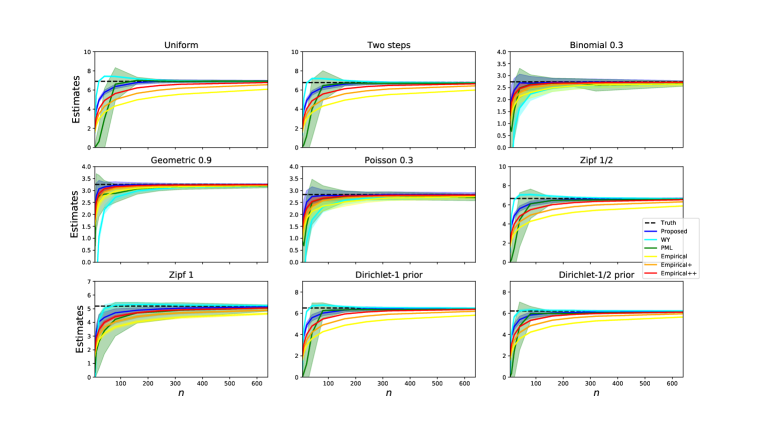
Figure 1: Shannon entropy

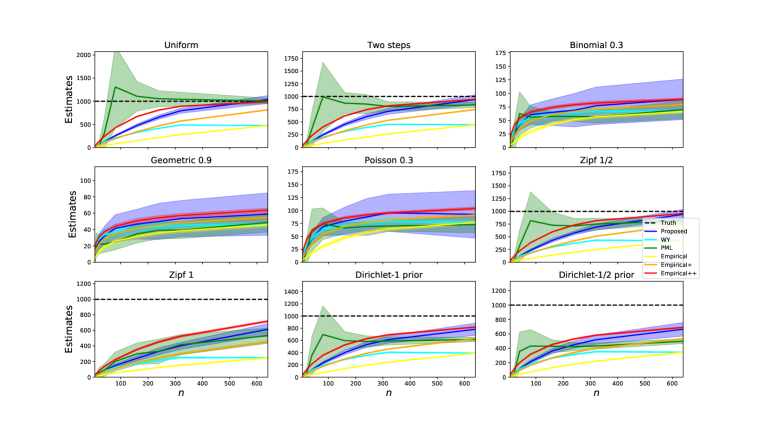
Figure 2: Support size

Appendix A A refined estimator for Shannon entropy

For $z\in[0,\infty]$, we define the following two $f$-functions:

$$f_{1}(z):=-e^{-z}\sum_{j=1}^{\infty}\frac{z^{j}}{j!}j\log j$$

and

$$f_{2}(z):=-e^{-z}\sum_{j=1}^{\infty}\frac{z^{j}}{j!}(j+1)\log(j+1).$$

A.1 Relating the $\boldsymbol{f}$-functions to Bernstein approximation errors

For $x\in[0,1]$, set $z=nx$. The following lemma relates ${f_{1}}(z)$ and ${f_{2}}(z)$ to $h_{n+1}(x)-B_{n}(h_{n+1},x)$.

Lemma 9.

For $x\in[0,{\log^{4}n}/{n}]$,

$$h_{n+1}(x)-B_{n}(h_{n+1},x)=(h(z+1)-{f_{2}}(z))-(h(z)-{f_{1}}(z))+\tilde{\mathcal{O}}\left(\frac{1}{n}\right).$$

Proof.

Let $h_{-1}(x):=h(x+n^{-1})$. By the linearity of expectation,

$$h_{n+1}(x)-B_{n}(h_{n+1},x) =n\left(h_{-1}(x)-h(x)-B_{n}(h_{-1},x)+B_{n}(h,x)\right)$$

$$=n\left(h_{-1}(x)-B_{n}(h_{-1},x)\right)-n\left(h(x)-B_{n}(h,x)\right).$$

Recall that $z=nx$, which implies $z\in[0,\log^{4}n]$. We have

$$n\left(h_{-1}(x)-B_{n}(h_{1},x)\right) =-(nx+1)\log\left(\frac{nx+1}{n}\right)+\sum_{j=0}^{n}(j+1)\log\left(\frac{j+1}{n}\right)\binom{n}{j}x^{j}(1-x)^{n-j}$$

$$=-(z+1)\log\left(\frac{z+1}{n}\right)+\sum_{j=0}^{n}(j+1)\log\left(\frac{j+1}{n}\right)\binom{n}{j}z^{j}\frac{(n-z)^{n-j}}{n^{n}}$$

$$=-(z+1)\log\left({z+1}\right)+\left(1-\frac{z}{n}\right)^{n}\sum_{j=0}^{n}(j+1)\log\left({j+1}\right)\binom{n}{j}z^{j}{(n-z)^{-j}}$$

$$=-(z+1)\log\left({z+1}\right)+\left(1-\frac{z}{n}\right)^{n}\sum_{j=0}^{n}(j+1)\log\left({j+1}\right)\frac{n^{\underline{j}}}{n^{j}}\frac{z^{j}}{j!}{\left(1-\frac{z}{n}\right)^{-j}}$$

$$=-(z+1)\log\left({z+1}\right)+e^{-z}\sum_{j=0}^{\infty}\frac{z^{j}}{j!}(j+1)\log(j+1)+\tilde{\mathcal{O}}\left(\frac{1}{n}\right)$$

$$=h(z+1)-{f_{2}}(z)+\tilde{\mathcal{O}}\left(\frac{1}{n}\right).$$

The second last equality is the most non-trivial step. To establish this equality, we need the following the three inequalities.

Inequality 1:

$$0\leq \left(1-\frac{z}{n}\right)^{n}\sum_{j=\log^{5}n+1}^{n}(j+1)\log\left({j+1}\right)\frac{n^{\underline{j}}}{n^{j}}\frac{z^{j}}{j!}{\left(1-\frac{z}{n}\right)^{-j}}$$

$$=\left(1-\frac{z}{n}\right)^{n}\sum_{j=\log^{5}n+1}^{n}(j+1)\log\left({j+1}\right)\frac{n^{\underline{j}}}{2^{j}(n-z)^{j}}\frac{(2z)^{j}}{j!}$$

$$\leq e^{-z}\sum_{j=\log^{5}n+1}^{n}(j+1)\log\left({j+1}\right)\frac{(2z)^{j}}{j!}$$

$$\leq e^{-z}\sum_{j=\log^{5}n+1}^{n}2j(j-1)\frac{(2z)^{j}}{j!}$$

$$\leq 8z^{2}e^{-z}\sum_{j=\log^{5}n-1}^{n}\frac{(2z)^{j}}{j!}$$

$$\leq 8(\log^{8}n)\Pr(\mathrm{Poi}(2z)\geq\log^{5}n-1)$$

$$\leq\frac{1}{n}.$$

Inequality 2:

$$0\leq e^{-z}\sum_{j=\log^{5}n+1}^{\infty}\frac{z^{j}}{j!}(j+1)\log(j+1)=2(\log^{8}n)\Pr(\mathrm{Poi}(2z)\geq\log^{5}n-1)\leq\frac{1}{n}.$$

Inequality 3:

For $j\leq\log^{5}n$,

$$\left|e^{-z}-\left(1-\frac{z}{n}\right)^{n}\frac{n^{\underline{j}}}{n^{j}}{\left(1-\frac{z}{n}\right)^{-j}}\right| =\left|e^{-z}-\left(1-\frac{z}{n}\right)^{n}\frac{n^{\underline{j}}}{(n-z)^{j}}\right|$$

$$\leq\left|e^{-z}-\left(1-\frac{z}{n}\right)^{n}\right|+\left(1-\frac{z}{n}\right)^{n}\left|1-\frac{n^{\underline{j}}}{(n-z)^{j}}\right|$$

$$\leq e^{-z}\frac{z^{2}}{n}+e^{-z}\left|1-\frac{n^{\underline{j}}}{(n-z)^{j}}\right|$$

$$\leq e^{-z}\frac{z^{2}}{n}+e^{-z}\left(\left|1-\frac{n^{j}}{(n-z)^{j}}\right|\lor\left|1-\frac{(n-\log^{5}n)^{j}}{(n-z)^{j}}\right|\right)$$

$$\leq e^{-z}\frac{z^{2}}{n}+e^{-z}\left(\left|\exp\left(\frac{zj}{n-z}\right)-1\right|\lor\left|\frac{(\log^{5}n-z){j}}{n-z}\right|\right)$$

$$\leq e^{-z}\frac{z^{2}}{n}+e^{-z}\left(\left|\frac{zj}{n-z(j+1)}\right|\lor\left|\frac{(\log^{5}n){j}}{n-z}\right|\right)$$

$$\leq e^{-z}\frac{2\log^{10}n}{n}.$$

Note that the last inequality implies

$$\left|e^{-z}\sum_{j=0}^{\log^{5}n}\frac{z^{j}}{j!}(j+1)\log(j+1)-\left(1-\frac{z}{n}\right)^{n}\sum_{j=0}^{\log^{5}n}(j+1)\log\left({j+1}\right)\frac{n^{\underline{j}}}{n^{j}}\frac{z^{j}}{j!}{\left(1-\frac{z}{n}\right)^{-j}}\right|$$

$$\leq\frac{2\log^{10}n}{n}\cdot e^{-z}\sum_{j=0}^{\log^{5}n}\frac{z^{j}}{j!}(2j(j-1))$$

$$\leq\frac{2\log^{10}n}{n}\cdot 2z^{2}$$

$$\leq\frac{4\log^{18}n}{n}.$$

This together with Inequality 1 and 2 proves the desired equality. Similarly, we have

$$n\left(h(x)-B_{n}(h,x)\right)=-z\log z+e^{-z}\sum_{j=1}^{\infty}\frac{z^{j}}{j!}j\log j+\tilde{\mathcal{O}}\left(\frac{1}{n}\right),$$

which completes the proof. ∎

For $x\in I_{n}$, let $z_{1}=(na-1)x$, then $z_{1}\in I_{n}^{\prime}:=[0,ac_{l}\log n]$. Hence by the above lemma,

$$h_{na}(x)-B_{na-1}(h_{na},x)=(h(z_{1}+1)-{f_{2}}(z_{1}))-(h(z_{1})-{f_{1}}(z_{1}))+\tilde{\mathcal{O}}\left(\frac{1}{n}\right).$$

In the next section, we approximate the function ${f_{1}}(z)$ with a degree-$d$ polynomial over $I_{n}^{\prime}$.

A.2 Approximating $\boldsymbol{{f_{1}}(z)}$

First consider the function

$${f_{1}}(z)=-e^{-z}\sum_{j=1}^{\infty}\frac{z^{j}}{j!}j\log j.$$

our objective is to approximate $f_{1}$ with a low-degree polynomial and bound the corresponding error. To do this, we first establish some basic properties of ${f_{1}}(z)$ in the next section.

A.2.1 Properties of $\boldsymbol{{f_{1}}(z)}$

Property 1:

The function ${f_{1}}(z)$ is a continuous function over $[0,\infty)$, and ${f_{1}}(0)=0$.

Property 2:

For all $z\geq 0$, the value of $f_{1}(z)$ is non-negative.

Property 3:

Denote

$$u(y):=(y+2)\log(y+2)+y\log y-2(y+1)\log(y+1).$$

Then, for $z\geq 0$,

$${f_{1}}^{\prime\prime}(z)=-e^{-z}\sum_{t=0}^{\infty}\frac{z^{t}}{t!}\cdot u(t).$$

Furthermore, we have

$$-\log 4\leq{f_{1}}^{\prime\prime}(z)<0.$$

Proof.

We prove the equality first.

$$-{f_{1}}^{\prime\prime}(z) =e^{-z}\sum_{t=1}^{\infty}\frac{(t-1)t^{2}z^{t-2}\log(t)}{t!}-2e^{-z}\sum_{t=1}^{\infty}\frac{t^{2}z^{t-1}\log(t)}{t!}+e^{-z}\sum_{t=1}^{\infty}\frac{tz^{t}\log(t)}{t!}$$

$$=e^{-z}\sum_{t=0}^{\infty}\frac{z^{t}(t+2)\log(t+2)}{t!}-2e^{-z}\sum_{t=0}^{\infty}\frac{z^{t}(t+1)\log(t+1)}{t!}+e^{-z}\sum_{t=0}^{\infty}\frac{tz^{t}\log(t)}{t!}$$

$$=e^{-z}\sum_{t=0}^{\infty}\frac{z^{t}}{t!}\cdot u(t).$$

To prove the inequality, we need the following lemma.

Lemma 10.

For $t\geq 0$,

$$\frac{\log 4}{t+1}\geq u(t)\geq\frac{1}{t+1}.$$

By Lemma 10, we have

$$0 <e^{-z}\sum_{t=0}^{\infty}\frac{z^{t}}{t!}\cdot\left(\frac{1}{t+1}\right)$$

$$\leq e^{-z}\sum_{t=0}^{\infty}\frac{z^{t}}{t!}\cdot u(t)$$

$$=-{f_{1}}^{\prime\prime}(z)$$

$$\leq e^{-z}\sum_{t=0}^{\infty}\frac{z^{t}}{t!}\cdot\frac{\log 4}{t+1}$$

$$=(\log 4)\frac{(1-e^{-z})}{z}$$

$$\leq\log 4.$$

∎

Property 4:

For $z>0$,

$$0\leq\frac{{f_{1}}^{\prime\prime}(z)}{h^{\prime\prime}(z)}\leq\log 4.$$

Proof.

Recall that $h(z)=-z\log z$,

$$h^{\prime\prime}(z)=-\frac{1}{z}$$

and thus

$$0 \leq\frac{{f_{1}}^{\prime\prime}(z)}{h^{\prime\prime}(z)}$$

$$=e^{-z}\sum_{t=0}^{\infty}\frac{z^{t+1}}{t!}\cdot u(t)$$

$$\leq e^{-z}\sum_{t=0}^{\infty}\frac{z^{t+1}}{t!}\cdot\frac{\log 4}{t+1}$$

$$\leq(\log 4)(1-e^{-z})$$

$$\leq\log 4,$$

where we have used Lemma 10 in the third step. ∎

A.2.2 Moduli of smoothness

In this section, we introduce some basic results in approximation theory [39]. For any function $f$ over $[0,1]$, let $\varphi(x)=\sqrt{x(1-x)}$, the first- and second- order Ditzian-Totik moduli of smoothness quantities of $f$ are

$$w^{1}_{\varphi}(f,t):=\sup\left\{|f(u)-f(v)|:0\leq u,v\leq 1,|u-v|\leq t\cdot\varphi\left(\frac{u+v}{2}\right)\right\},$$

and

$$w^{2}_{\varphi}(f,t):=\sup\left\{\left|f(u)+f(v)-2f\left(\frac{u+v}{2}\right)\right|:0\leq u,v\leq 1,|u-v|\leq 2t\cdot\varphi\left(\frac{u+v}{2}\right)\right\},$$

respectively. For any integer $m\geq 1$ and any function $f$ over $[0,1]$, let $P_{m}$ be the collection of degree-$m$ polynomials, and

$$E_{m}[f]:=\min_{g\in P_{m}}\max_{x\in[0,1]}|f(x)-g(x)|$$

be the maximum approximation error of the degree-$m$ min-max polynomial of $f$. The relation between the best polynomial-approximation error $E_{m}[f]$ of a continuous function $f$ and the smoothness quantity $w^{2}_{\varphi}(f,t)$ is established in the following lemma [39].

Lemma 11.

There are absolute constants $C_{1}$ and $C_{2}$ such that for any continuous function $f$ over $[0,1]$ and any $m>2$,

$$E_{m}[f]\leq C_{1}w^{2}_{\varphi}(f,m^{-1}),$$

and

$$\frac{1}{m^{2}}\sum_{t=0}^{m}(t+1)E_{t}[f]\geq C_{2}w^{2}_{\varphi}(f,m^{-1}).$$

The above lemma shows that $w^{2}_{\varphi}(f,\boldsymbol{\cdot})$ essentially characterizes $E_{\boldsymbol{\cdot}}[f]$.

A.2.3 Bounding the error in approximating $\boldsymbol{{f_{1}}(x)}$

For simplicity, we define $x^{\prime}:=(ac_{l}\log n)\cdot x$ and consider the following function.

$${f_{1^{\prime}}}(x):={f_{1}}((ac_{l}\log n)\cdot x).$$

Approximating ${f_{1}}(x^{\prime})$ over $I_{n}^{\prime}=[0,ac_{l}\log n]$ is equivalent to approximate ${f_{1^{\prime}}}(x)$ over the unit interval $[0,1]$. According to Lemma 11, to bound $E_{d}[{f_{1^{\prime}}}]$, it suffices to bound $w^{2}_{\varphi}({f_{1^{\prime}}},\boldsymbol{\cdot})$. Specifically, we know that

$$\min_{g\in P_{d}}\max_{x\in I_{n}^{\prime}}|{f_{1}}(x)-g(x)|=E_{d}[{f_{1^{\prime}}}]\leq C_{1}w^{2}_{\varphi}({f_{1^{\prime}}},d^{-1}).$$

Note that by definition, $w^{2}_{\varphi}({f_{1^{\prime}}},d^{-1})$ is the solution to the following optimization problem.

$$\sup_{u,v}\left|{f_{1^{\prime}}}(u)+{f_{1^{\prime}}}(v)-2{f_{1^{\prime}}}\left(\frac{u+v}{2}\right)\right|$$

subject to

$$0\leq u,v\leq 1,|u-v|\leq\frac{2}{d}\cdot\varphi\left(\frac{u+v}{2}\right).$$

Consider the optimization constraints first. Following [6], we denote $M:=(u+v)/2$ and $\delta:=d^{-1}\sqrt{1/M-1}$. The feasible region can be written as

$$[M-d^{-1}\sqrt{M(1-M)},M+d^{-1}\sqrt{M(1-M)}]\cap[0,1]=[M-\delta M,M+\delta M]\cap[0,1].$$

By Property 3 in Section A.2.1, ${f_{1}}(x^{\prime})$, or equivalently ${f_{1^{\prime}}}(x)$, is a strictly concave function. Therefore, the maximum of $\left|f(u)+f(v)-2f({u+v}/{2})\right|$ is attained at the boundary of the feasible region. Noting that

$$M-d^{-1}\sqrt{M(1-M)}\geq 0\iff M\geq\frac{1}{d^{2}+1}$$

and

$$M+d^{-1}\sqrt{M(1-M)}\leq 1\iff M\leq\frac{d^{2}}{d^{2}+1},$$

we only need to consider the following three cases:

Case 1:

$$u=0,v=2M,M\in[0,{1}/{(d^{2}+1)}].$$

Case 2:

$$u=2M-1,v=1,M\in[{d^{2}}/{(d^{2}+1)},1].$$

Case 3:

$$u=M-\delta M,v=M+\delta M,M\in[{1}/{(d^{2}+1)},{d^{2}}/{(d^{2}+1)}].$$

To facilitate our derivations, we need the following lemma.

Lemma 12.

Let $f\in C^{1}([a,b])$ have second order derivative in $(a,b)$. There exists $c\in(a,b)$ such that

$$f(a)+f(b)-2f\left(\frac{a+b}{2}\right)=\frac{1}{4}(b-a)^{2}\cdot f^{\prime\prime}(c).$$

First consider Case 1. By the above lemma, there exists $c\in(0,{2}/{(d^{2}+1)})$ such that

$$\left|{f_{1^{\prime}}}(0)+{f_{1^{\prime}}}\left(\frac{2}{d^{2}+1}\right)-2{f_{1^{\prime}}}\left(\frac{1}{d^{2}+1}\right)\right|\leq\frac{1}{4}\cdot\left(\frac{2}{d^{2}+1}\right)^{2}\left|{f_{1^{\prime}}}^{\prime\prime}(c)\right|=\left(\frac{1}{d^{2}+1}\right)^{2}\left|{f_{1^{\prime}}}^{\prime\prime}(c)\right|.$$

By definition,

$$|{f_{1^{\prime}}}^{\prime\prime}(x)|=|(ac_{l}\log n)^{2}g_{1}^{\prime\prime}((ac_{l}\log n)\cdot x)|\leq(\log 4)(ac_{l}\log n)^{2}.$$

Hence,

$$\left(\frac{1}{d^{2}+1}\right)^{2}\left|{f_{1^{\prime}}}^{\prime\prime}(c)\right|\leq\mathcal{O}\left(\varepsilon^{2}\right).$$

This, together with an analogous argument for Case 2, implies that the objective value is bounded by $\mathcal{O}\left(\varepsilon^{2}\right)$ in both cases. It remains to analyze Case 3. We consider two regimes:

Regime 1:

If $M\leq 4/(d^{2}+1)$, then $|u-v|=2d^{-1}\sqrt{M(1-M)}\leq 4/d^{2}$. The above derivations again give us

$$\left|{f_{1^{\prime}}}(u)+{f_{1^{\prime}}}(v)-2{f_{1^{\prime}}}\left(\frac{u+v}{2}\right)\right|\leq\mathcal{O}\left(\varepsilon^{2}\right).$$

Regime 2:

If $4/(d^{2}+1)\leq M\leq{d^{2}}/{(d^{2}+1)}$, then

$$M-\delta M=M\left(1-\frac{\sqrt{M^{-1}-1}}{d}\right)\geq M\left(1-\frac{\sqrt{(d^{2}+1)-4}}{2d}\right)\geq\frac{M}{2}.$$

By Lemma 12, there exists $c\in(M-\delta M,M+\delta M)\subseteq(M/2,3M/2)$ such that

$$\left|{f_{1^{\prime}}}(u)+{f_{1^{\prime}}}(v)-2{f_{1^{\prime}}}\left(\frac{u+v}{2}\right)\right|\leq\frac{1}{4}\cdot\left(2\frac{1}{d}\sqrt{M(1-M)}\right)^{2}\cdot\left|{f_{1^{\prime}}}^{\prime\prime}(c)\right|.$$

By Property 4 in Section A.2.1,

$$|{f_{1^{\prime}}}^{\prime\prime}(c)|=|(ac_{l}\log n)^{2}f_{1}^{\prime\prime}((ac_{l}\log n)\cdot c)|\leq(ac_{l}\log n)^{2}\cdot(\log 4)\cdot\frac{1}{(ac_{l}\log n)\cdot c}\leq(\log 8)\cdot\frac{ac_{l}\log n}{M}.$$

This immediately implies

$$\frac{1}{4}\cdot\left(2\frac{1}{d}\sqrt{M(1-M)}\right)^{2}\cdot\left|{f_{1^{\prime}}}^{\prime\prime}(c)\right|\leq\frac{1}{d^{2}}M(1-M)\cdot(\log 8)\cdot\frac{ac_{l}\log n}{M}\leq(\log 8)\cdot\frac{c_{l}\varepsilon}{c_{s}^{2}}.$$

Consolidating all the previous results, we get

$$\min_{g\in P_{d}}\max_{x\in I_{n}^{\prime}}|{f_{1}}(x)-g(x)|\leq\mathcal{O}\left(\varepsilon\right).$$

Similarly, for the function ${f_{2}}$, we also have

$$\min_{g\in P_{d}}\max_{x\in I_{n}^{\prime}}|{f_{2}}(x)-g(x)|\leq\mathcal{O}\left(\varepsilon\right).$$

In the next section, we use these two inequalities to analyze our refined entropy estimator.

A.3 Constructing the refined estimator

For our purpose, we need to approximate $B_{na-1}(h_{na},x)-h_{na}(x)$ over the interval $I_{n}=[0,c_{l}\log n/n]$ by a degree-$d$ polynomial. By Lemma 9, for $x\in I_{n}$ and $z_{1}:=(na-1)x\in I_{n}^{\prime}=[0,ac_{l}\log n]$,

$$h_{na}(x)-B_{na-1}(h_{na},x)=(h(z_{1}+1)-{f_{2}}(z_{1}))-(h(z_{1})-{f_{1}}(z_{1}))+\tilde{\mathcal{O}}\left(\frac{1}{n}\right).$$

By the results in [40],

$$\min_{g\in P_{d}}\max_{x\in I_{n}^{\prime}}|h(x)-g(x)| =(ac_{l}\log n)\min_{g\in P_{d}}\max_{x\in[0,1]}|h(x)-g(x)|$$

$$\leq\mathcal{O}\left(\frac{ac_{l}\log n}{(c_{s}\log n)^{2}}\right)$$

$$\leq\mathcal{O}\left(\varepsilon\right)$$

and

$$\min_{g\in P_{d}}\max_{x\in I_{n}^{\prime}}|h(x+1)-g(x)|\leq\mathcal{O}\left(\varepsilon\right).$$

Combining these bounds with the last two inequalities in the last section, we get

$$\min_{g\in P_{d-1}}\max_{x\in I_{n}}|(h_{na}(x)-B_{na-1}(h_{na},x))-g(x)|\leq\mathcal{O}\left(\varepsilon\right).$$

Let $\tilde{g}(x)$ be the min-max polynomial that achieves the above minimum. By the derivations in Section 4.2, the degree-$(d-1)$ polynomial $\tilde{h}_{na}(x)$ satisfies

$$\max_{x\in I_{n}}|h_{na}(x)-\tilde{h}_{na}(x)|\leq\mathcal{O}\left(\varepsilon\right).$$

Denote $\tilde{h}^{*}(x):=-\tilde{g}(x)+\tilde{h}_{na}(x)$, and note that by definition, $B_{na}^{\prime}(h,x)=B_{na-1}(h_{na},x)$. The triangle inequality implies

$$\max_{x\in I_{n}}|B_{na}^{\prime}(h,x)-\tilde{h}^{*}(x)|=\max_{x\in I_{n}}|B_{na-1}(h_{na},x)-\tilde{h}^{*}(x)|\leq\mathcal{O}\left(\varepsilon\right).$$

By a simple argument, the degree-$d$ polynomial

$$\tilde{H}^{*}(x):=\int_{0}^{x}\tilde{h}^{*}(t)dt,$$

approximates $B_{na}(h,x)$ with the following pointwise error guarantee.

Lemma 13.

For any $x\in I_{n}$,

$$|B_{na}(h,x)-\tilde{H}^{*}(x)|\leq\mathcal{O}\left(x\epsilon\right).$$

In other words, $\tilde{H}^{*}(x)$ is a degree-$d$ polynomial that well approximates $B_{na}(h,x)$ pointwisely.

Next we argue that the coefficients of $\tilde{H}^{*}(x)$ can not be too large. For notational convenience, let $\tilde{h}^{*}(x)=\sum_{v=0}^{d-1}a_{v}x^{v}$. By Corollary 2, for $x\in I_{n}$,

$$|h_{na}(x)-B_{na-1}(h_{na},x)|\leq 1.$$

Furthermore, for $x\in I_{n}$, $h_{na}(x)$ is an increasing function and thus

$$|h_{na}(x)|=\max\left\{|h_{na}(0)|,h_{na}\left(\frac{c_{l}(\log n)}{n}\right)\right\}\leq\mathcal{O}(\log n).$$

Hence, over $I_{n}$,

$$|\tilde{h}^{*}(x)|\leq\mathcal{O}(\log n).$$

Due to the boundedness of $\tilde{h}^{*}(x)$, its coefficients cannot be too large:

$$|a_{v}|\leq\mathcal{O}\left(2^{4.5d}\log n\right)\left(\frac{n}{c_{l}\log n}\right)^{v}.$$

Write $\tilde{H}^{*}(x)$ as $\tilde{H}^{*}(x)=\sum_{t=1}^{d}a_{t}^{\prime}x^{t}$. Then by $\tilde{H}^{*}(x):=\int_{0}^{x}\tilde{h}^{*}(t)dt$ and the above bound on $|a_{v}|$,

$$|a_{t}^{\prime}|\leq\left(\frac{n}{c_{l}\log n}\right)^{t-1}\mathcal{O}(2^{4.5d}).$$

The construction of the new entropy estimator follows by replacing $\tilde{H}_{na}(x)$ with $\tilde{H}^{*}(x)$ in Section 5. The rest of the proof is almost the same as that in the main paper and thus is omitted.

Appendix B Competitive estimators for general additive properties

Consider an arbitrary real function $f:[0,1]\to\mathbb{R}$. Without loss of generality, we assume that $f(0)=0$. According to the previous derivations, we can write $B_{n}^{\prime}(f,x)$ as

$$B_{n}^{\prime}(f,x):=\sum_{j=0}^{n-1}n\left(f\left(\frac{j+1}{n}\right)-f\left(\frac{j}{n}\right)\right)\binom{n-1}{j}x^{j}(1-x)^{(n-1)-j}.$$

Our objective is to approximate $B_{na}^{\prime}(f,x)$ with a low degree polynomial. For now, let us assume that $f$ is a $1$-Lipschitz function. For $x\in[0,1]$, set $z=nx$. Denote $g_{n+1}(j):=(n+1)f\left(\frac{j}{n+1}\right)$,

$$f_{1,n+1}(z):=e^{-z}\sum_{j=0}^{\infty}g_{n+1}(j+1)\frac{z^{j}}{j!},$$

and

$$f_{2,n+1}(z):=e^{-z}\sum_{j=0}^{\infty}g_{n+1}(j)\frac{z^{j}}{j!}$$

The following lemma relates $f_{1,n+1}(z)$ and $f_{2,n+1}(z)$ to $B_{n+1}^{\prime}(f,x)$.

Lemma 14.

For $x\in[0,{\log^{4}n}/{n}]$,

$$B_{n+1}^{\prime}(f,x)=f_{1,n+1}(z)-f_{2,n+1}(z)+\tilde{\mathcal{O}}\left(\frac{1}{n}\right).$$

Proof.

By definition $z=nx$, hence $z\in[0,\log^{4}n]$. We have

$$\sum_{j=0}^{n}(n+1)f\left(\frac{j+1}{n+1}\right)\binom{n}{j}x^{j}(1-x)^{n-j} =\sum_{j=0}^{n}g_{n+1}(j+1)\binom{n}{j}z^{j}\frac{(n-z)^{n-j}}{n^{n}}$$

$$=\left(1-\frac{z}{n}\right)^{n}\sum_{j=0}^{n}g_{n+1}(j+1)\binom{n}{j}z^{j}{(n-z)^{-j}}$$

$$=\left(1-\frac{z}{n}\right)^{n}\sum_{j=0}^{n}g_{n+1}(j+1)\frac{n^{\underline{j}}}{n^{j}}\frac{z^{j}}{j!}{\left(1-\frac{z}{n}\right)^{-j}}$$

$$=e^{-z}\sum_{j=0}^{\infty}g_{n+1}(j+1)\frac{z^{j}}{j!}+\tilde{\mathcal{O}}\left(\frac{1}{n}\right)$$

$$=f_{1,n+1}(z)+\tilde{\mathcal{O}}\left(\frac{1}{n}\right).$$

The second last equality is the most non-trivial step. To establish this equality, we need the following the three inequalities.

Inequality 1:

$$0\leq \left(1-\frac{z}{n}\right)^{n}\sum_{j=\log^{5}n+1}^{n}|g_{n+1}(j+1)|\frac{n^{\underline{j}}}{n^{j}}\frac{z^{j}}{j!}{\left(1-\frac{z}{n}\right)^{-j}}$$

$$=\left(1-\frac{z}{n}\right)^{n}\sum_{j=\log^{5}n+1}^{n}(j+1)\frac{n^{\underline{j}}}{2^{j}(n-z)^{j}}\frac{(2z)^{j}}{j!}$$

$$\leq e^{-z}\sum_{j=\log^{5}n+1}^{n}(j+1)\frac{(2z)^{j}}{j!}$$

$$\leq e^{-z}\sum_{j=\log^{5}n+1}^{n}2j(j-1)\frac{(2z)^{j}}{j!}$$

$$\leq 8z^{2}e^{-z}\sum_{j=\log^{5}n-1}^{n}\frac{(2z)^{j}}{j!}$$

$$\leq 8(\log^{8}n)\Pr(\mathrm{Poi}(2z)\geq\log^{5}n-1)$$

$$\leq\frac{1}{n}.$$

Inequality 2:

$$0\leq e^{-z}\sum_{j=\log^{5}n+1}^{\infty}|g_{n+1}(j+1)|\frac{z^{j}}{j!}\leq e^{-z}\sum_{j=\log^{5}n+1}^{\infty}(j+1)\frac{z^{j}}{j!}\leq\frac{1}{n}.$$

Inequality 3:

For $j\leq\log^{5}n$,

$$\left|e^{-z}-\left(1-\frac{z}{n}\right)^{n}\frac{n^{\underline{j}}}{n^{j}}{\left(1-\frac{z}{n}\right)^{-j}}\right| =\left|e^{-z}-\left(1-\frac{z}{n}\right)^{n}\frac{n^{\underline{j}}}{(n-z)^{j}}\right|$$

$$\leq\left|e^{-z}-\left(1-\frac{z}{n}\right)^{n}\right|+\left(1-\frac{z}{n}\right)^{n}\left|1-\frac{n^{\underline{j}}}{(n-z)^{j}}\right|$$

$$\leq e^{-z}\frac{z^{2}}{n}+e^{-z}\left|1-\frac{n^{\underline{j}}}{(n-z)^{j}}\right|$$

$$\leq e^{-z}\frac{z^{2}}{n}+e^{-z}\left(\left|1-\frac{n^{j}}{(n-z)^{j}}\right|\lor\left|1-\frac{(n-\log^{5}n)^{j}}{(n-z)^{j}}\right|\right)$$

$$\leq e^{-z}\frac{z^{2}}{n}+e^{-z}\left(\left|\exp\left(\frac{zj}{n-z}\right)-1\right|\lor\left|\frac{(\log^{5}n-z){j}}{n-z}\right|\right)$$

$$\leq e^{-z}\frac{z^{2}}{n}+e^{-z}\left(\left|\frac{zj}{n-z(j+1)}\right|\lor\left|\frac{(\log^{5}n){j}}{n-z}\right|\right)$$

$$\leq e^{-z}\frac{2\log^{10}n}{n}.$$

Note that the last inequality implies

$$\left|e^{-z}\sum_{j=0}^{\log^{5}n}\frac{z^{j}}{j!}g_{n+1}(j+1)-\left(1-\frac{z}{n}\right)^{n}\sum_{j=0}^{\log^{5}n}g_{n+1}(j+1)\frac{n^{\underline{j}}}{n^{j}}\frac{z^{j}}{j!}{\left(1-\frac{z}{n}\right)^{-j}}\right|$$

$$\leq\frac{2\log^{10}n}{n}\cdot e^{-z}\sum_{j=0}^{\log^{5}n}\frac{z^{j}}{j!}(j+1)$$

$$\leq\frac{2\log^{10}n}{n}\cdot(1+2z)$$

$$\leq\frac{5\log^{14}n}{n}.$$

This together with Inequality 1 and 2 proves the desired equality. Similarly, we have

$$\sum_{j=0}^{n}(n+1)f\left(\frac{j}{n+1}\right)\binom{n}{j}x^{j}(1-x)^{n-j}=f_{2,n+1}(z)+\tilde{\mathcal{O}}\left(\frac{1}{n}\right).$$

This completes the proof. ∎ Re-define $z:=(na-1)x$. Lemma 14 immediately implies that for $x\in I_{n}=[0,c_{l}(\log n)/n]\subseteq[0,{(\log^{4}(na-1))}/{(na-1)}]$,

$$B_{na}^{\prime}(f,x)=f_{1,na}(z)-f_{2,na}(z)+\tilde{\mathcal{O}}\left(\frac{1}{na}\right).$$

Note that in this case $z\in I_{n}^{\prime}=[0,ac_{l}\log n]$. Let $t_{na}(z):=f_{1,na}(z)-f_{2,na}(z)$ and $r_{na}(j):=g_{na}(j+2)+g_{na}(j)-2g_{na}(j+1)$. Then direct calculation yields,

$$t^{\prime\prime}_{na}(z) =e^{-z}\sum_{j=0}^{\infty}r_{na}(j+1)\frac{z^{j}}{j!}-e^{-z}\sum_{j=0}^{\infty}r_{na}(j)\frac{z^{j}}{j!}$$

$$=e^{-z}\sum_{j=0}^{\infty}r_{na}(j+1)\frac{z^{j}}{j!}-e^{-z}r_{na}(0)-\sum_{j=0}^{\infty}r_{na}(j+1)\frac{z^{j+1}}{(j+1)!}$$

$$=e^{-z}\sum_{j=0}^{\infty}r_{na}(j+1)\left(\frac{z^{j}}{j!}-\frac{z^{j+1}}{(j+1)!}\right)-e^{-z}r_{na}(0)$$

Since we assume that $f$ is $1$-Lipschitz, $|r_{na}(j)|\leq 2$. Therefore, for $z\in I_{n}^{\prime}$,

$$|t^{\prime\prime}_{na}(z)| \leq e^{-z}\sum_{j=0}^{\infty}|r_{na}(j+1)|\left(\frac{z^{j}}{j!}+\frac{z^{j+1}}{(j+1)!}\right)+e^{-z}|r_{na}(0)|\leq 6.$$

We can bound each individual term by the following lemma.

Lemma 15.

For $j\geq 1$ and $z\geq 0$, we have

$$\left|e^{-z}\left(\frac{z^{j}}{j!}-\frac{z^{j+1}}{(j+1)!}\right)\right|\leq\frac{1}{\sqrt{2\pi}((j+1)-\sqrt{j+1})}$$

and

$$\left|e^{-z}\left(\frac{z^{j}}{j!}-\frac{z^{j+1}}{(j+1)!}\right)\right|\leq\frac{5}{z}.$$

Proof.

Let us denote

$$q_{1}(z):=e^{-z}\left(\frac{z^{j}}{j!}-\frac{z^{j+1}}{(j+1)!}\right).$$

The derivative of $q_{1}(z)$ is

$$q^{\prime}_{1}(z) =-e^{-z}\frac{z^{j}}{j!}+e^{-z}\frac{z^{j-1}}{(j-1)!}+e^{-z}\frac{z^{j+1}}{(j+1)!}-e^{-z}\frac{z^{j}}{j!}$$

$$=e^{-z}\frac{z^{j-1}}{(j+1)!}\left(-2(j+1)z+j(j+1)+z^{2}\right).$$

Set $q^{\prime}_{1}(z)=0$ and note that $q_{1}(0)=\lim_{z\to\infty}q_{1}(z)=0$, the maximum of $|q_{1}(z)|$ is attained at $z_{1}:=(j+1)-\sqrt{j+1}$ or $z_{2}:=(j+1)+\sqrt{j+1}$. We consider $z_{1}$ first.

$$|q_{1}(z_{1})| =e^{-z_{1}}\frac{z_{1}^{j+1}}{(j+1)!}\left|\frac{j+1}{z_{1}}-1\right|$$

$$\leq e^{-(j+1)+\sqrt{j+1}}((j+1)-\sqrt{j+1})^{j+1}\frac{e^{j+1}}{\sqrt{2\pi}(j+1)^{j+1+1/2}}\frac{1}{\sqrt{j+1}-1}$$

$$\leq e^{\sqrt{j+1}}\left(1-\frac{1}{\sqrt{j+1}}\right)^{j+1}\frac{1}{\sqrt{2\pi}\sqrt{j+1}}\frac{1}{\sqrt{j+1}-1}$$

$$\leq\frac{1}{\sqrt{2\pi}((j+1)-\sqrt{j+1})}.$$

Similarly, for $z_{2}$, we also have $|q_{1}(z_{1})|\leq{1}/{(\sqrt{2\pi}((j+1)+\sqrt{j+1}))}$. Analogously, let us denote

$$q_{2}(z):=e^{-z}\left(\frac{z^{j+1}}{j!}-\frac{z^{j+2}}{(j+1)!}\right).$$

The derivative of $q_{2}(z)$ is

$$q^{\prime}_{2}(z) =e^{-z}\frac{z^{j}}{(j+1)!}\left(-(2j+3)z+(j+1)^{2}+z^{2}\right).$$

Set $q^{\prime}_{2}(z)=0$ and note that $q_{2}(0)=\lim_{z\to\infty}q_{2}(z)=0$, the maximum of $|q_{2}(z)|$ is attained at $z_{3}:=((2j+3)-\sqrt{4j+5})/2$ or $z_{4}:=((2j+3)+\sqrt{4j+5})/2$. Note that $|z_{3}|,|z_{4}|\leq 2(j+2)$. Therefore,

$$|q_{2}(z_{3})|=|z_{3}||q_{1}(z_{3})|\leq 2(j+2)\max_{z}|q_{1}(z)|\leq\frac{2(j+2)}{\sqrt{2\pi}((j+1)-\sqrt{j+1})}\leq 5,\forall j\geq 1.$$

The same proof also shows that $|q_{2}(z_{4})|\leq 5$. ∎

B.1 $\ell_{1}$-distance

Now let us focus on the problem of estimating the $\ell_{1}$-distance between the unknown distribution $\vec{p}\in\Delta_{k}$ and a given distribution $\vec{q}\in\Delta_{k}$. Since our estimator is constructed symbol by symbol, it is sufficient to consider the problem of approximating $\ell_{q}(x)=|x-q|-q$.

Set $g_{n+1}(j):=(n+1)\ell_{q}\left(\frac{j}{n+1}\right)$. We note that $r_{na}(j)$ equals $0$ for all but at most two different values of $j$. Therefore, by Lemma 15, for all $z\in I_{n}^{\prime}$, we have $|t^{\prime\prime}_{na}(z)|\leq\mathcal{O}(1)$, and $|t^{\prime\prime}_{na}(z)|\leq\mathcal{O}(1)z^{-1}$, where the first and second inequalities resemble Property 3 and 4 in Section A.2.1, respectively. Using arguments similar to those in Section A.2.3 and A.3, we can construct an estimator for $D_{\vec{q}}(\vec{p})$ that provides the guarantees stated in Theorem 2. Note that concavity/convexity is actually not crucial to establishing the final result in Section A.2.3. Also note that we need to replace our analysis in Section 6.2 and 7.2 for the corresponding large-probability estimator by that in [7].

B.2 General additive properties

More generally, the results on $\ell_{1}$-distance hold for any additive property $F(\vec{p})=\sum_{i\in[k]}f_{i}(p_{i})$ that satisfies the simple condition: $f_{i}$ is $\mathcal{O}(1)$-Lipschitz, for all $i$. Without loss of generality, assume that all $f_{i}$’s are $1$-Lipschitz and satisfy $f_{i}(0)=0$. By the previous derivations, we immediately have $|t^{\prime\prime}_{na}(z)|\leq 6$, which recovers Property 3 in Section A.2.3. Again, concavity/convexity is actually not necessary to establishing the final result in Section A.2.3. The proof will be complete if we also recover Property 4 in that section. In other words, we only need to show: $|t^{\prime\prime}_{na}(z)z|\leq\mathcal{O}(1)$, where

$$t^{\prime\prime}_{na}(z)z=e^{-z}\sum_{j=0}^{\infty}r_{na}(j+1)\left(\frac{z^{j+1}}{j!}-\frac{z^{j+2}}{(j+1)!}\right)-e^{-z}zr_{na}(0).$$

Fix $z\in I_{n}^{\prime}$ and treat it as a constant. Let $b_{j}:=r_{na}(j+1)$ and $a_{j}:=e^{-z}\left(\frac{z^{j+1}}{j!}-\frac{z^{j+2}}{(j+1)!}\right)$. By Lemma 15, we have $|a_{j}|\leq 5,\forall j\geq 1$. Note that there is need to worry about the slack term $e^{-z}zr_{na}(0)$ and the first term in the sum which corresponds to $j=0$, since the absolute values of both terms contribute at most $\mathcal{O}(1)$ to the expression for any $z\geq 0$. The key observation is that any consecutive partial sum of sequence $\{b_{j}\}_{j\geq 1}$ is also bounded by $\mathcal{O}(1)$ in magnitude. Specifically, for any $n_{1},n_{2}\in\mathbb{Z}^{+}$ satisfying $n_{1}+2\leq n_{2}$,

$$\left|\sum_{j=n_{1}}^{n_{2}}b_{j}\right| =\left|\sum_{j=n_{1}}^{n_{2}}r_{na}(j+1)\right|$$

$$=\left|\sum_{j=n_{1}}^{n_{2}}(g_{na}(j+3)+g_{na}(j+1)-2g_{na}(j+2))\right|$$

$$=\left|\sum_{j=n_{1}+3}^{n_{2}+3}g_{na}(j)+\sum_{j=n_{1}+1}^{n_{2}+1}g_{na}(j)-2\sum_{j=n_{1}+2}^{n_{2}+2}g_{na}(j)\right|$$

$$=\left|(g_{na}(n_{2}+3)-g_{na}(n_{2}+2))+(g_{na}(n_{1}+1)-g_{na}(n_{1}+2))\right|$$

$$\leq 2.$$

Furthermore, the sequence $\{a_{j}\}_{j\geq 1}$ can change its monotonicity at most two times. We can prove this claim by considering the sign of $a_{j}-a_{j-1}$. More concretely,

$$\operatorname{sign}\left(a_{j}-a_{j-1}\right) =\operatorname{sign}\left(e^{-z}\left(\frac{z^{j+1}}{j!}-\frac{z^{j+2}}{(j+1)!}\right)-e^{-z}\left(\frac{z^{j}}{(j-1)!}-\frac{z^{j+1}}{j!}\right)\right)$$

$$=\operatorname{sign}\left(2(j+1)z-z^{2}-(j+1)j\right)$$

$$=\operatorname{sign}\left(-j^{2}+j(2z-1)+(2z-z^{2})\right).$$

Since $z$ is fixed, the last expression can change its value at most two times as $j$ increases from $0$ to infinity. The last piece of the proof is the following corollary of the well-known Abel’s inequality.

Lemma 16.

Let $\{a^{\prime}_{j}\}_{j=1}^{m}$ be a sequence of real numbers that is either increasing or decreasing, and let $\{b^{\prime}_{j}\}_{j=1}^{m}$ be a sequence of real or complex numbers. Then,

$$|\sum_{j=1}^{m}a^{\prime}_{j}b^{\prime}_{j}|\leq\max_{t=1,\ldots,m}|B^{\prime}_{t}|(2|a^{\prime}_{n}|+|a^{\prime}_{1}|),$$

where $B^{\prime}_{t}:=\sum_{j=1}^{t}b^{\prime}_{t}$.

By the previous discussion, we can find two indices $j_{1}$ and $j_{2}$, such that $\{a_{j}\}_{j=1}^{j_{1}}$, $\{a_{j}\}_{j=j_{1}+1}^{j_{2}}$, and $\{a_{j}\}_{j\geq j_{2}+1}$ are all monotone subsequences. Then, we apply Lemma 16 to each of them and further bound the resulting quantities by the two inequalities proved above: $\left|\sum_{j=n_{1}}^{n_{2}}b_{j}\right|\leq\mathcal{O}(1)$ and $|a_{j}|\leq 6,\forall j\geq 1$. This concludes the proof. Finally, we would like to point out that the above argument actually applies to a much broader class of additive properties beyond the Lipschitz one, which we will not address here for the sake of clarity and simplicity.

Appendix C A competitive estimator for support size

C.1 Estimator construction

Recall that

$$s(x)=\mathds{1}_{x>0}.$$

Let $\vec{p}$ and $S_{\vec{p}}$ denote an unknown distribution and its support size. Re-define $a:=|\log^{-2}\epsilon|\cdot\log S_{\vec{p}}$. Let $X^{na}$ be a sample sequence drawn from $\vec{p}$, and $N_{i}^{\prime\prime}$ be the number of times symbol $i$ appears.

The $na$-sample empirical estimator estimates the support size by

$$\hat{S}^{E}(X^{na}):=\sum_{i\in[k]}\mathds{1}_{N_{i}^{\prime\prime}>0}.$$

Taking expectation, we have

$$\mathbb{E}[\hat{S}^{E}(X^{na})]:=\sum_{i\in[k]}\mathbb{E}[\mathds{1}_{N_{i}^{\prime\prime}>0}]=\sum_{i\in[k]}(1-(1-p_{i})^{na}).$$

Following [3, 4], having a length-$\mathrm{Poi}(n)$ sample $X^{N}$, we denote by $\phi_{j}$ the number of symbols that appear $j$ times and estimate $\mathbb{E}[\hat{S}^{E}(X^{na})]$ by

$$\hat{S}(X^{N}):=\sum_{j=1}^{\infty}\phi_{j}(1-(-(a-1))^{j}\Pr(Z\geq j)),$$

where $Z\sim\mathrm{Poi}(r)$ for some parameter $r$. In addition, we define $N_{i}$ as the number of times symbol $i$ appears. By the property of Poisson sampling, all the $N_{i}$’s are independent.

C.2 Bounding the bias

The following lemma bounds the bias of $\hat{S}(X^{N})$ in estimating $\mathbb{E}[\hat{S}^{E}(X^{na})]$.

Lemma 17.

For all $a\geq 1$,

$${|\mathbb{E}[\hat{S}(X^{N})]-\mathbb{E}[\hat{S}^{E}(X^{na})]|}\leq\min\left\{na,S_{\vec{p}}\right\}e^{-r}+2.$$

Proof.

Noting that for any $m\geq 0$ and $p\in[0,1]$,

$$0\leq e^{-mp}-(1-p)^{m}\leq 2p,$$

we have

$${|\mathbb{E}[\hat{S}(X^{N})]-\mathbb{E}[\hat{S}^{E}(X^{na})]|}$$

$$=\left|\mathbb{E}\left[\sum_{j}^{\infty}\phi_{j}\right]-\mathbb{E}\left[\sum_{j}^{\infty}\phi_{j}(-(a-1))^{j}\Pr(Z\geq j)\right]-\sum_{i\in[k]}(1-(1-p_{i})^{na})\right|$$

$$=\left|\sum_{i\in[k]}(1-e^{-np_{i}})-\mathbb{E}\left[\sum_{j}^{\infty}\phi_{j}(-(a-1))^{j}\Pr(Z\geq j)\right]-\sum_{i\in[k]}(1-(1-p_{i})^{na})\right|$$

$$\leq\left|\sum_{i\in[k]}(-e^{-np_{i}})-\mathbb{E}\left[\sum_{j}^{\infty}\phi_{j}(-(a-1))^{j}\Pr(Z\geq j)\right]-\sum_{i\in[k]}(-e^{-nap_{i}})\right|+2\sum_{i\in[k]}p_{i}$$

$$=\left|\sum_{i\in[k]}e^{-np_{i}}(e^{-n(a-1)p_{i}}-1)-\mathbb{E}\left[\sum_{j}^{\infty}\phi_{j}(-(a-1))^{j}\Pr(Z\geq j)\right]\right|+2$$

$$\leq\min\left\{na,S_{\vec{p}}\right\}e^{-r}+2,$$

where the last step follows by Lemma 7 and Corollary 2 in [4]. ∎

C.3 Bounding the mean absolute deviation

C.3.1 Bounds for $\boldsymbol{\hat{S}(X^{N})}$

In this section, we analyze the mean absolute deviation of $\hat{S}(X^{N})$. To do this, we need the following two lemmas. The first lemma bounds the coefficients of this estimator.

Lemma 18.

[3] For $j\geq 1$ and $a\geq 1$,

$$|1-(-(a-1))^{j}\Pr(Z\geq j)|\leq 1+e^{r(a-1)}.$$

The second lemma is the McDiarmid’s inequality.

Lemma 19.

Let ${Y_{1},\ldots,Y_{m}}$ be independent random variables taking values in ranges ${R_{1},\ldots,R_{m}}$, and let $F:R_{1}\times\ldots\times R_{m}\rightarrow C$ with the property that if one freezes all but the ${w^{th}}$ coordinate of ${F(y_{1},\ldots,y_{m})}$ for some ${1\leq w\leq m}$, then ${F}$ only fluctuates by most ${c_{w}>0}$, thus $|F(y_{1},\ldots,y_{w-1},y_{w},\\ y_{w+1},\ldots,y_{m})-F(y_{1},\ldots,y_{w-1},y_{w}^{\prime},y_{w+1},\ldots,y_{m})|\leq c_{w}$ for all ${y_{j}\in R_{j}}$ and ${y^{\prime}_{w}\in R_{w}}$ for ${1\leq j\leq m}$. Then for any ${\lambda>0}$, one has $\displaystyle\Pr(|F(Y)-\mathbb{E}[F(Y)]|\geq\lambda\sigma)\leq C\exp(-c\lambda^{2})$ for some absolute constants ${C,c>0}$, where ${\sigma^{2}:=\sum_{j=1}^{m}c_{j}^{2}}$.

Note that $\hat{S}(X^{N})$, when viewed as a function of $N_{i}$’s with indexes $i$ satisfying $p_{i}\not=0$, fullfills the property described in Lemma 19, with $m=S_{\vec{p}}$ and $c_{w}=2+2e^{r(a-1)}$ for all $1\leq w\leq m$. Therefore, for $\sigma^{2}:=4S_{\vec{p}}(1+e^{r(a-1)})^{2}$,

$$\Pr(|\hat{S}(X^{N})-\mathbb{E}[\hat{S}(X^{N})]|\geq\lambda\sigma)\leq C\exp(-c\lambda^{2}).$$

This further implies

$$\mathbb{E}\left|\hat{S}(X^{N})-\mathbb{E}[\hat{S}(X^{N})]\right| =\int_{0}^{\infty}\Pr(|\hat{S}(X^{N})-\mathbb{E}[\hat{S}(X^{N})]|\geq t)\ dt$$

$$=\sigma\int_{0}^{\infty}\Pr(|\hat{S}(X^{N})-\mathbb{E}[\hat{S}(X^{N})]|\geq\lambda\sigma)\ d\lambda$$

$$\leq C\sigma\int_{0}^{\infty}\exp(-c\lambda^{2})d\lambda$$

$$\leq\mathcal{O}(\sqrt{S_{\vec{p}}}(1+e^{r(a-1)})).$$

Analogously, viewing $\hat{S}(X^{N})$ as a function of $X_{i}$’s implies

$$\mathbb{E}\left|\hat{S}(X^{N})-\mathbb{E}[\hat{S}(X^{N})]\right|\leq\mathcal{O}(\sqrt{n}(1+e^{r(a-1)})).$$

Hence,

$$\mathbb{E}\left|\hat{S}(X^{N})-\mathbb{E}[\hat{S}(X^{N})]\right|\leq\mathcal{O}\left(\sqrt{\min\left\{S_{\vec{p}},n\right\}}(1+e^{r(a-1)})\right).$$

C.3.2 Bounds for $\boldsymbol{\hat{S}^{E}(X^{na})}$

The following lemma bounds the variance of $\hat{S}^{E}(X^{na})$ in terms of $S_{\vec{p}}$.

Lemma 20.

For $m\geq 1$ and $X^{m}\sim\vec{p}$,

$$\mathrm{Var}(\hat{S}^{E}(X^{m}))\leq\mathcal{O}(S_{\vec{p}}).$$

Proof.

Let $N_{i}$ denote the number of times symbol $i$ appears in $X^{m}$. By independence,

$$\mathrm{Var}(\hat{S}^{E}(X^{m})) =\mathrm{Var}\left(\sum_{i:p_{i}>0}\mathds{1}_{N_{i}>0}\right)$$

$$=\mathbb{E}\left[\left(\sum_{i:p_{i}>0}\mathds{1}_{N_{i}>0}\right)^{2}\right]-\left(\mathbb{E}\left[\sum_{i:p_{i}>0}\mathds{1}_{N_{i}>0}\right]\right)^{2}$$

Let $M\sim\mathrm{Poi}(m)$ and $X^{M}$ be an independent sample of length $M$. Let $N_{i}^{\prime}$ denote the number of times symbol $i$ appears in $X^{M}$. We have

$$\mathbb{E}\left[\left(\sum_{i:p_{i}>0}\mathds{1}_{N_{i}>0}\right)^{2}\right]$$

$$=\mathbb{E}\left[\sum_{i:p_{i}>0}\mathds{1}_{N_{i}>0}+\sum_{i\not=j:p_{i}>0,p_{j}>0}\mathds{1}_{N_{i}>0}\mathds{1}_{N_{j}>0}\right]$$

$$=\sum_{i:p_{i}>0}(1-\mathbb{E}[\mathds{1}_{N_{i}=0}])+\sum_{i\not=j:p_{i}>0,p_{j}>0}\mathbb{E}[(1-\mathds{1}_{N_{i}=0})(1-\mathds{1}_{N_{j}=0})]$$

$$=\sum_{i:p_{i}>0}(1-(1-p_{i})^{m})+\sum_{i\not=j:p_{i}>0,p_{j}>0}\left(1-(1-p_{i})^{m}-(1-p_{j})^{m}+(1-p_{i}-p_{j})^{m}\right)$$

Noting that for any $m\geq 0$ and $p\in[0,1]$,

$$0\leq e^{-mp}-(1-p)^{m}\leq 2p,$$

we have

$$|(1-(1-p_{i})^{m})-(1-e^{-mp_{i}})|\leq 2p_{i}$$

and

$$|(1-(1-p_{i})^{m}-(1-p_{j})^{m}+(1-p_{i}-p_{j})^{m})-(1-e^{-mp_{i}}-e^{-mp_{j}}+e^{-m(p_{i}+p_{j})})|\leq 4(p_{i}+p_{j}).$$

Therefore,

$$\left|\mathbb{E}\left[\left(\sum_{i:p_{i}>0}\mathds{1}_{N_{i}>0}\right)^{2}\right]-\mathbb{E}\left[\left(\sum_{i:p_{i}>0}\mathds{1}_{N_{i}^{\prime}>0}\right)^{2}\right]\right| \leq\sum_{i:p_{i}>0}2p_{i}+\sum_{i\not=j:p_{i}>0,p_{j}>0}4(p_{i}+p_{j})$$

$$\leq 4\sum_{i:p_{i}>0}\sum_{j:p_{j}>0}(p_{i}+p_{j})$$

$$\leq 8S_{\vec{p}}.$$

Similarly,

$$\left|\left(\mathbb{E}\left[\sum_{i:p_{i}>0}\mathds{1}_{N_{i}>0}\right]\right)^{2}-\left(\mathbb{E}\left[\sum_{i:p_{i}>0}\mathds{1}_{N_{i}^{\prime}>0}\right]\right)^{2}\right|$$

$$=\left|\mathbb{E}\left[\sum_{i:p_{i}>0}\mathds{1}_{N_{i}>0}\right]-\mathbb{E}\left[\sum_{i:p_{i}>0}\mathds{1}_{N_{i}^{\prime}>0}\right]\right|\left|\mathbb{E}\left[\sum_{i:p_{i}>0}\mathds{1}_{N_{i}>0}\right]+\mathbb{E}\left[\sum_{i:p_{i}>0}\mathds{1}_{N_{i}^{\prime}>0}\right]\right|$$

$$\leq\left|\sum_{i:p_{i}>0}\mathbb{E}\left[\mathds{1}_{N_{i}>0}\right]-\sum_{i:p_{i}>0}\mathbb{E}\left[\mathds{1}_{N_{i}^{\prime}>0}\right]\right|\cdot 2S_{\vec{p}}$$

$$\leq(\sum_{i:p_{i}>0}2p_{i})\cdot 2S_{\vec{p}}$$

$$\leq 4S_{\vec{p}}.$$

Note that changing the value of a particular $N_{i}^{\prime}$ changes the value of $\sum_{i:p_{i}>0}\mathds{1}_{N_{i}^{\prime}>0}$ by at most $1$. Again, by the McDiarmid’s inequality,

$$\mathrm{Var}\left(\sum_{i:p_{i}>0}\mathds{1}_{N_{i}^{\prime}>0}\right)\leq\mathcal{O}(S_{\vec{p}}).$$

The triangle inequality combines all the above results and yields

$$\mathrm{Var}\left(\sum_{i:p_{i}>0}\mathds{1}_{N_{i}>0}\right)\leq\mathcal{O}(S_{\vec{p}}).$$

∎

By Jensen’s inequality, the above lemma implies

$$\mathbb{E}\left|\hat{S}^{E}(X^{na})-\mathbb{E}[\hat{S}^{E}(X^{na})]\right|\leq\sqrt{\mathrm{Var}(\hat{S}^{E}(X^{na}))}\leq\mathcal{O}(\sqrt{S_{\vec{p}}}).$$

C.4 Proving Theorem 4

Setting $r=|\log\epsilon|$, we get

$$e^{r(a-1)}\leq{S_{\vec{p}}^{|\log^{-1}\epsilon|}}$$

and

$$e^{-r}=e^{-|\log\epsilon|}=\epsilon.$$

Hence, by the previous results,

$$\mathbb{E}\left|\hat{S}(X^{N})-\hat{S}^{E}(X^{na})\right| \leq\mathbb{E}\left|\hat{S}(X^{N})-\mathbb{E}[\hat{S}^{E}(X^{na})]\right|+\mathbb{E}\left|\mathbb{E}[\hat{S}^{E}(X^{na})]-\hat{S}^{E}(X^{na})\right|$$

$$\leq\mathcal{O}\left(S_{\vec{p}}^{|\log^{-1}\epsilon|+\frac{1}{2}}+S_{\vec{p}}\cdot\varepsilon\right).$$

Normalize both sides by $S_{\vec{p}}$. Then,

$$\mathbb{E}\left[\left|\frac{\hat{S}(X^{N})}{S_{\vec{p}}}-\frac{\hat{S}^{E}(X^{na})}{S_{\vec{p}}}\right|\right]\leq\mathcal{O}\left({S_{\vec{p}}^{|\log^{-1}\epsilon|-\frac{1}{2}}}+\varepsilon\right).$$

Appendix D A competitive estimator for support coverage

D.1 Estimator construction

Recall that

$$c(p):=1-(1-p_{i})^{m},$$

where $m$ is a given parameter. Re-define the amplification parameter as $a:=|\log^{-2}\epsilon|\cdot\log C_{\vec{p}}$. Similar to the last section, let $X^{na}$ be an independent length-$na$ sample sequence drawn from $\vec{p}$, and $N_{i}^{\prime\prime}$ be the number of times symbol $i$ appears.

The $na$-sample empirical estimator estimates $C_{\vec{p}}=\sum_{i\in[k]}c(p_{i})$ by the quantity

$$\hat{C}^{E}(X^{na}):=\sum_{i\in[k]}c(N_{i}^{\prime\prime}/(na))=\sum_{i\in[k]}\left(1-\left(1-\frac{N_{i}^{\prime\prime}}{na}\right)^{m}\right).$$

Taking expectation, we get

$$\mathbb{E}[\hat{C}^{E}(X^{na})]=\sum_{i\in[k]}\mathbb{E}\left[1-\left(1-\frac{N_{i}^{\prime\prime}}{na}\right)^{m}\right].$$

Let us denote

$$T(\vec{p}):=\sum_{i\in[k]}\mathbb{E}\left[1-e^{-m\frac{N_{i}^{\prime\prime}}{na}}\right].$$

Noting that for $t\geq 1$ and $p\in[0,1]$,

$$|e^{-tp}-(1-p)^{t}|\leq 2p,$$

we have

$$|\mathbb{E}[\hat{C}^{E}(X^{na})]-T(\vec{p})]\leq\sum_{i\in[k]}\mathbb{E}\left[2\cdot\frac{N_{i}^{\prime\prime}}{na}\right]=2.$$

Thus, it suffices to estimate $T(\vec{p})$, which satisfies

$$T(\vec{p}) =\sum_{i\in[k]}\left(1-\mathbb{E}\left[e^{-m\frac{N_{i}^{\prime\prime}}{na}}\right]\right)$$

$$=\sum_{i\in[k]}\left(1-\sum_{j=0}^{na}\binom{na}{j}p_{i}^{j}(1-p_{i})^{na-j}e^{-m\frac{j}{na}}\right)$$

$$=\sum_{i\in[k]}\left(1-\sum_{j=0}^{na}\binom{na}{j}\left(p_{i}\cdot e^{-\frac{m}{na}}\right)^{j}(1-p_{i})^{na-j}\right)$$

$$=\sum_{i\in[k]}\left(1-\left(1-p_{i}(1-e^{-\frac{m}{na}})\right)^{na}\right).$$

Let us denote

$$T_{1}(\vec{p}):=\sum_{i\in[k]}\left(1-\exp\left(-na(1-e^{-\frac{m}{na}})p_{i}\right)\right).$$

Since $(1-e^{-\frac{m}{na}})p_{i}\in[0,1]$, we have

$$|T(\vec{p})-T_{1}(\vec{p})|\leq\sum_{i\in[k]}2(1-e^{-\frac{m}{na}})p_{i}\leq 2.$$

Define a new amplification parameter $a^{\prime}:=a(1-e^{-\frac{m}{na}})$. We can write $T_{1}(\vec{p})$ as

$$T_{1}(\vec{p}):=\sum_{i\in[k]}\left(1-\exp\left(-na^{\prime}p_{i}\right)\right).$$

For simplicity, we assume that $m\geq 1.5n$ and $a>1.8$. Then

$$a^{\prime}=a(1-e^{-\frac{m}{na}})\geq a(1-e^{-\frac{1.5}{a}})>1.$$

Analogous to case of support size estimation, we can draw a length-$\mathrm{Poi}(n)$ sample sequence $X^{N}$ and estimate $\mathbb{E}[\hat{C}^{E}(X^{na})]$ by

$$\hat{C}(X^{N}):=\sum_{j=1}^{\infty}\phi_{j}(1-(-(a^{\prime}-1))^{j}\Pr(\mathrm{Poi}(r)\geq j)).$$

D.2 Bounding the bias

We bound the bias of $\hat{C}(X^{N})$ in estimating $\mathbb{E}[\hat{C}^{E}(X^{na})]$ as follows.

$$|\mathbb{E}[\hat{C}(X^{N})]-\mathbb{E}[\hat{C}^{E}(X^{na})]| \leq|\mathbb{E}[\hat{C}(X^{N})]-T_{1}(\vec{p})|+|T_{1}(\vec{p})-\mathbb{E}[\hat{C}^{E}(X^{na})]|$$

$$\leq|\mathbb{E}[\hat{C}(X^{N})]-T_{1}(\vec{p})|+4$$

$$=\left|\sum_{i\in[k]}e^{-np_{i}}(e^{-n(a^{\prime}-1)p_{i}}-1)\right.$$

$$\left.-\sum_{i\in[k]}e^{-np_{i}}\sum_{j=1}^{\infty}\frac{(-(a^{\prime}-1)np_{i})^{j}}{j!}\Pr(\mathrm{Poi}(r)\geq j)\right|+4$$

$$\leq\left|\sum_{i\in[k]}e^{-np_{i}}\left(\sum_{j=1}^{\infty}\frac{(-(a^{\prime}-1)np_{i})^{j}}{j!}\Pr(\mathrm{Poi}(r)<j)\right)\right|+4.$$

To bound the last sum, we need the following lemma.

Lemma 21.

For all $y,r\geq 0$,

$$\left|\sum_{j=1}^{\infty}\frac{(-y)^{j}}{j!}\Pr(\mathrm{Poi}(r)<j)\right|\leq e^{-r}(1-e^{-y}).$$

Proof.

By Lemma 6 of [4],

$$\left|\sum_{j=1}^{\infty}\frac{(-y)^{j}}{j!}\Pr(\mathrm{Poi}(r)<j)\right| \leq\max_{s\leq y}\left|\mathbb{E}_{L\sim\mathrm{Poi}(r)}\left[\frac{(-s)^{L}}{L!}\right]\right|(1-e^{-y})$$

$$=\max_{s\leq y}\left|J_{0}(2\sqrt{sr})\right|e^{-r}(1-e^{-y})$$

$$\leq e^{-r}(1-e^{-y}),$$

where $J_{0}$ is the Bessel function of the first kind and satisfies $|J_{0}(x)|\leq 1,\forall x\geq 0$ [41]. ∎

By the above lemma, we have

$$|\mathbb{E}[\hat{C}(X^{N})]-\mathbb{E}[\hat{C}^{E}(X^{na})]| \leq\left|\sum_{i\in[k]}e^{-np_{i}}\left(\sum_{j=1}^{\infty}\frac{(-(a^{\prime}-1)np_{i})^{j}}{j!}\Pr(\mathrm{Poi}(r)<j)\right)\right|+4$$

$$\leq e^{-r}\sum_{i\in[k]}e^{-np_{i}}(1-e^{-(a^{\prime}-1)np_{i}})+4$$

$$\leq e^{-r}\sum_{i\in[k]}(1-e^{-na^{\prime}p_{i}})+4.$$

Note that $na^{\prime}=na(1-e^{-\frac{m}{na}})\leq m$. Hence,

$${|\mathbb{E}[\hat{C}(X^{N})]-\mathbb{E}[\hat{C}^{E}(X^{na})]|}\leq e^{-r}\sum_{i\in[k]}(1-e^{-mp_{i}})+4=e^{-r}C_{\vec{p}}+4.$$

D.3 Bounding the mean absolute deviation

D.3.1 Bounds for $\boldsymbol{\hat{C}(X^{N})}$

Now we bound the mean absolute deviation of $\hat{C}(X^{N})$ in terms of $C_{\vec{p}}$. By the Jensen’s inequality,

$$\mathbb{E}\left|\hat{C}(X^{N})-\mathbb{E}[\hat{C}(X^{N})]\right| \leq\sqrt{\mathrm{Var}\left(\hat{C}(X^{N})\right)}$$

$$=\sqrt{\sum_{i\in k}\mathrm{Var}\left({\sum_{j=1}^{\infty}\mathds{1}_{N_{i}=j}(1-(-(a^{\prime}-1))^{j}\Pr(\mathrm{Poi}(r)\geq j))}\right)}$$

$$\leq\sqrt{\sum_{i\in k}\mathbb{E}\left[\left(\sum_{j=1}^{\infty}\mathds{1}_{N_{i}=j}(1-(-(a^{\prime}-1))^{j}\Pr(\mathrm{Poi}(r)\geq j))\right)^{2}\right]}$$

$$=\sqrt{\sum_{i\in k}\sum_{j=1}^{\infty}\mathbb{E}\left[\mathds{1}_{N_{i}=j}\right]\left(1-(-(a^{\prime}-1))^{j}\Pr(\mathrm{Poi}(r)\geq j)\right)^{2}}$$

$$\leq(1+e^{r(a^{\prime}-1)})\sqrt{\sum_{i\in k}(1-e^{-np_{i}})}$$

By our assumption that $m\geq 1.5n$,

$$\mathbb{E}[|\hat{C}(X^{N})-\mathbb{E}[\hat{C}(X^{N})]|] \leq(1+e^{r(a^{\prime}-1)})\sqrt{\sum_{i\in k}(1-e^{-np_{i}})}$$

$$\leq(1+e^{r(a^{\prime}-1)})\sqrt{\sum_{i\in k}(1-e^{-mp_{i}})}$$

$$\leq(1+e^{r(a^{\prime}-1)})\sqrt{\sum_{i\in k}(1-(1-p_{i})^{m})}$$

$$=(1+e^{r(a^{\prime}-1)})\sqrt{C_{\vec{p}}}.$$

D.3.2 Bounds for $\boldsymbol{\hat{C}^{E}(X^{na})}$

It remains to bound the mean absolute deviation of the $na$-sample empirical estimator. To deal with the dependence among the counts $N_{i}^{\prime\prime}$’s, we need the following definition and lemma [42].

Definition 1.

Random variables $X_{1},\ldots,X_{S}$ are said to be negatively associated if for any pair of disjoint subsets $A_{1},A_{2}$ of ${1,2,\ldots,S}$, and any component-wise increasing functions $f_{1},f_{2}$,

$$\text{Cov}(f_{1}(X_{i},i\in A_{1}),f_{2}(X_{j},j\in A_{2}))\leq 0.$$

Next lemma can be used to check whether random variables are negatively associated or not.

Lemma 22.

Let $X_{1},\ldots,X_{S}$ be $S$ independent random variables with log-concave densities. Then the joint conditional distribution of $X_{1},\ldots,X_{S}$ given $\sum_{i=1}^{S}X_{i}$ is negatively associated.

By Lemma 22, $N_{i}^{\prime\prime}$’s are negatively correlated. Furthermore, note that

$$c^{*}(x):=1-\left(1-\frac{x}{na}\right)^{m}$$

is an increasing function, and

$$\hat{C}^{E}(X^{na}):=\sum_{i\in[k]}c^{*}(N_{i}^{\prime\prime}).$$

Hence for any $i,j\in[k]$ such that $i\not=j$,

$$\text{Cov}(c^{*}(N_{i}^{\prime\prime}),c^{*}(N_{j}^{\prime\prime}))\leq 0.$$

Therefore,

$$\mathrm{Var}\left(\hat{C}^{E}(X^{na})\right) =\sum_{i\in[k]}\mathrm{Var}(c^{*}(N_{i}^{\prime\prime}))+2\sum_{i,j\in[k],i\not=j}\text{Cov}(c^{*}(N_{i}^{\prime\prime}),c^{*}(N_{j}^{\prime\prime}))$$

$$\leq\sum_{i\in[k]}\mathrm{Var}(c^{*}(N_{i}^{\prime\prime}))$$

$$\leq\sum_{i\in[k]}\mathbb{E}[(c^{*}(N_{i}^{\prime\prime}))^{2}]$$

$$=\sum_{i\in[k]}\mathbb{E}\left[\sum_{j=0}^{na}\mathds{1}_{N_{i}=j}(C^{*}(j))^{2}\right]$$

$$\leq\sum_{i\in[k]}\sum_{j=1}^{na}\mathbb{E}\left[\mathds{1}_{N_{i}=j}\right]$$

$$=\sum_{i\in[k]}(1-(1-p_{i})^{na}).$$

Without loss of generality, we can assume that $a$ is a positive integer. Then,

$$\sum_{i\in[k]}(1-(1-p_{i})^{na}) =\sum_{i\in[k]}(1-(1-p_{i})^{n})(\sum_{j=0}^{a-1}(1-p_{i})^{nj})$$

$$\leq a\sum_{i\in[k]}(1-(1-p_{i})^{n})$$

$$\leq a\sum_{i\in[k]}(1-(1-p_{i})^{m})$$

$$=aC_{\vec{p}}.$$

The Jensen’s inequality implies that

$$\mathbb{E}\left|\hat{C}^{E}(X^{na})-\mathbb{E}[\hat{C}^{E}(X^{na})]\right|\leq\sqrt{\mathrm{Var}(\hat{C}^{E}(X^{na}))}\leq\sqrt{aC_{\vec{p}}}.$$

D.4 Proving Theorem 5

The triangle inequality consolidates the major inequalities above and yields

$$\mathbb{E}\left|\hat{C}(X^{N})-\hat{C}^{E}(X^{na})\right|\leq\mathcal{O}\left(e^{-r}C_{\vec{p}}+4+\sqrt{aC_{\vec{p}}}+(1+e^{r(a^{\prime}-1)})\sqrt{C_{\vec{p}}}\right).$$

Using the fact that $a^{\prime}<a=|\log^{-2}\epsilon|\cdot\log C_{\vec{p}}$ and set $r=|\log\epsilon|$, we get

$$\mathbb{E}\left|\hat{C}(X^{N})-\hat{C}^{E}(X^{na})\right|\leq\mathcal{O}\left(\varepsilon C_{\vec{p}}+4+(1+C_{\vec{p}}^{{|\log^{-1}\epsilon|}}+\sqrt{\log C_{\vec{p}}})\sqrt{C_{\vec{p}}}\right).$$

Normalize both sides by $C_{\vec{p}}$. Then,

$$\mathbb{E}\left|\frac{\hat{C}(X^{N})}{C_{\vec{p}}}-\frac{\hat{C}^{E}(X^{na})}{C_{\vec{p}}}\right|\leq\mathcal{O}\left(C_{\vec{p}}^{|\log^{-1}\epsilon|-\frac{1}{2}}+\varepsilon\right).$$

References

• [1] P. Valiant and G. Valiant. Estimating the unseen: improved estimators for entropy and other properties. In Advances in Neural Information Processing Systems, pages 2157–2165, 2013.
• [2] Y. Wu and P. Yang. Minimax rates of entropy estimation on large alphabets via best polynomial approximation. IEEE Transactions on Information Theory, 62(6):3702–3720, 2016.
• [3] J. Acharya, H. Das, A. Orlitsky, and A. T. Suresh. A unified maximum likelihood approach for estimating symmetric properties of discrete distributions. In International Conference on Machine Learning, pages 11–21, 2017.
• [4] A. Orlitsky, A. T. Suresh, and Y. Wu. Optimal prediction of the number of unseen species. Proceedings of the National Academy of Sciences, 113(47):13283–13288, 2016.
• [5] Y. Wu and P. Yang. Chebyshev polynomials, moment matching, and optimal estimation of the unseen. The Annals of Statistics, 47(2), 2019.
• [6] J. Jiao, K. Venkat, Y. Han, and T. Weissman. Minimax estimation of functionals of discrete distributions. IEEE Transactions on Information Theory, 61(5):2835–2885, 2015.
• [7] Y. Hao, A. Orlitsky, A. T. Suresh, and Y. Wu. Data amplification: A unified and competitive approach to property estimation supplementary. In Advances in Neural Information Processing Systems, pages 8848–8857, 2018.
• [8] W. A. Gale and G. Sampson. Good-Turing frequency estimation without tears. Journal of Quantitative Linguistics, 3(2):217–237, 1995.
• [9] T. M. Cover and J. A. Thomas. Elements of information theory. John Wiley & Sons, 2012.
• [10] C. Chow and C. Liu. Approximating discrete probability distributions with dependence trees. IEEE Transactions on Information Theory, 14(3):462–467, 1968.
• [11] C. J. Quinn, N. Kiyavash, and T. P. Coleman. Efficient methods to compute optimal tree approximations of directed information graphs. IEEE Transactions on Signal Processing, 61(12):3173–3182, 2013.
• [12] G. Bresler. Efficiently learning Ising models on arbitrary graphs. In Proceedings of the 47th Annual ACM Symposium on Theory of Computing, pages 771–782. ACM, 2015.
• [13] W. Gerstner and W. M. Kistler. Spiking neuron models: Single neurons, populations, plasticity. Cambridge University Press, 2002.
• [14] Z. F. Mainen and T. J. Sejnowski. Reliability of spike timing in neocortical neurons. Science, 268(5216):1503–1506, 1995.
• [15] Van Steveninck, R. R. D. R., G. D. Lewen, S. P. Strong, R. Koberle, and W. Bialek. Reproducibility and variability in neural spike trains. Science, 275(5307):1805–1808, 1997.
• [16] T. Batu, L. Fortnow, R. Rubinfeld, W. D. Smith, and P. White. Testing that distributions are close. In Proceedings 41st Annual Symposium on Foundations of Computer Science, pages 259–269. IEEE, 2000.
• [17] T. Batu, E. Fischer, L. Fortnow, R. Kumar, R. Rubinfeld, and P. White. Testing random variables for independence and identity. In Proceedings of 42nd IEEE Symposium on Foundations of Computer Science, pages 442–451. IEEE, 2001.
• [18] D. Ron. Algorithmic and analysis techniques in property testing. Number 5 in 2. Foundations and Trends in Theoretical Computer Science, 2010.
• [19] C. L. Canonne. A survey on distribution testing: Your data is big. But is it blue? 2017.
• [20] D. R. McNeil. Estimating an author’s vocabulary. Journal of the American Statistical Association, 68(341):92–96, 1973.
• [21] R. Thisted and B. Efron. Did Shakespeare write a newly-discovered poem? Biometrika, 74(3):445–455, 1987.
• [22] B. Efron and R. Thisted. Estimating the number of unseen species: How many words did Shakespeare know? Biometrika, 63(3):435–447, 1976.
• [23] C. X. Mao and B. G. Lindsay. Estimating the number of classes. The Annals of Statistics, pages 917–930, 2007.
• [24] I. J. Good. The population frequencies of species and the estimation of population parameters. Biometrika, 40(3-4):237–264, 1953.
• [25] R. K. Colwell, A. Chao, N. J. Gotelli, S. Y. Lin, C. X. Mao, R. L. Chazdon, and J. T. Longino. Models and estimators linking individual-based and sample-based rarefaction, extrapolation and comparison of assemblages. Journal of Plant Ecology, 5(1):3–21, 2012.
• [26] A. Chao. Nonparametric estimation of the number of classes in a population. Scandinavian Journal of Statistics, pages 265–270, 1984.
• [27] A. Chao and S. M. Lee. Estimating the number of classes via sample coverage. Journal of the American Statistical Association, 87(417):210–217, 1992.
• [28] A. Chao and C. H. Chiu. Species richness: estimation and comparison. Wiley StatsRef: Statistics Reference Online, pages 1–26, 2014.
• [29] I. Kroes, P. W. Lepp, and D. A. Relman. Bacterial diversity within the human subgingival crevice. Proceedings of the National Academy of Sciences, 96(25):14547–14552, 1999.
• [30] A. Chao. Nonparametric estimation of the number of classes in a population. Scandinavian Journal of Statistics, pages 265–270, 1984.
• [31] I. Ionita-Laza, C. Lange, and N. M. Laird. Estimating the number of unseen variants in the human genome. Proceedings of the National Academy of Sciences, 106(13):5008–5013, 2009.
• [32] P. J. Haas, J. F. Naughton, S. Seshadri, and L. Stokes. Sampling-based estimation of the number of distinct values of an attribute. VLDB, 95:311–322, 1995.
• [33] A. Orlitsky and A. T. Suresh. Competitive distribution estimation: Why is Good-Turing good. In Advances in Neural Information Processing Systems, pages 2143–2151, 2015.
• [34] G. Valiant and P. Valiant. Instance optimal learning of discrete distributions. In Proceedings of the 48th Annual ACM Symposium on Theory of Computing, pages 142–155. ACM, 2016.
• [35] L. Paninski. Estimation of entropy and mutual information. Neural Computation, 15(6):1191–1253, 2003.
• [36] F. R. Chung and L. Lu. Complex graphs and networks, volume 107. American Mathematical Soc., 2017.
• [37] J. Bustamante. Bernstein operators and their properties. Chicago., 2017.
• [38] H. Berens, G. G. Lorentz, and R. E. MacKenzie. Inverse theorems for Bernstein polynomials. Indiana University Mathematics Journal, 21(8):693–708, 1972.
• [39] Z. Ditzian and V. Totik. Moduli of smoothness, volume 9. Springer Science & Business Media, 2012.
• [40] N. P Kornĕichuk. Exact constants in approximation theory, volume 38. Cambridge University Press, 1991.
• [41] M. Abramowitz and I. A. Stegun. Handbook of mathematical functions with formulas, graphs, and mathematical tables. Wiley-Interscience, New York, NY, 1964.
• [42] K. Joag-Dev and F. Proschan. Negative association of random variables with applications. The Annals of Statistics, 11(1):286–295, 1983.