Modules for Experiments in Stellar Astrophysics (MESA): Pulsating Variable Stars, Rotation, Convective Boundaries, and Energy Conservation

Abstract

We update the capabilities of the open-knowledge software instrument Modules for Experiments in Stellar Astrophysics (MESA). RSP is a new functionality in MESAstar that models the non-linear radial stellar pulsations that characterize RR Lyrae, Cepheids, and other classes of variable stars. We significantly enhance numerical energy conservation capabilities, including during mass changes. For example, this enables calculations through the He flash that conserve energy to better than 0.001%. To improve the modeling of rotating stars in MESA, we introduce a new approach to modifying the pressure and temperature equations of stellar structure, and a formulation of the projection effects of gravity darkening. A new scheme for tracking convective boundaries yields reliable values of the convective-core mass, and allows the natural emergence of adiabatic semiconvection regions during both core hydrogen- and helium-burning phases. We quantify the parallel performance of MESA on current generation multicore architectures and demonstrate improvements in the computational efficiency of radiative levitation. We report updates to the equation of state and nuclear reaction physics modules. We briefly discuss the current treatment of fallback in core-collapse supernova models and the thermodynamic evolution of supernova explosions. We close by discussing the new MESA Testhub software infrastructure to enhance source-code development.

1 Introduction

One of the foundations upon which modern astrophysics rests is the fundamental properties of stars throughout their evolution. The advent of transformative capabilities in space- and ground-based hardware instruments is providing an unprecedented volume of high-quality measurements of stars, significantly strengthening and extending the observational data upon which all of stellar astrophysics ultimately depends. For example, the Parker Solar Probe will provide new information on the flow of energy, structure, and dynamics of the closest star (Parker, 1958a; Feng et al., 2010; Cranmer & Winebarger, 2018; Gombosi et al., 2018) and the Daniel K. Inouye Solar Telescope will provide high temporal and spatial resolution with adaptive optics to reveal the nature of the the outer layers of the Sun (Parker, 1958b; Snow et al., 2018; McComas et al., 2018).

The exceptional precision of stellar brightness measurements achieved by the planet-hunting space telescopes Kepler/K2 (Borucki et al., 2010; Howell et al., 2014) and CoRoT (Auvergne et al., 2009) ushered in a new era in stellar photometric variability investigations. The Transiting Exoplanet Survey Satellite is building upon this legacy by surveying most of the sky in roughly month-long sectors covering four 24^∘ $\times$ 24^∘ areas from the ecliptic poles to near the ecliptic plane (Ricker et al., 2016). The mission will produce light curves for about 200,000 nearby late-type stars sampled at a 2 minute cadence to open a new era of stellar variability exploration (e.g., Dragomir et al., 2019; Huang et al., 2018; Ball et al., 2018; Shen et al., 2018; Wang et al., 2019). The Characterizing Exoplanets Satellite will complement these surveys by providing a unique, large sample of high precision photometric monitoring of selected bright target stars (Broeg et al., 2013; Gaidos et al., 2017).

The Gaia Data Release 2, containing about 1.7 billion stars, begins the process of converting the spectrophotometric measurements to distances, proper motions, luminosities, effective temperatures, surface gravities, and elemental compositions (Gaia Collaboration et al., 2018a; Bailer-Jones et al., 2018; Lindegren et al., 2018; Luri et al., 2018). This stellar census will revolutionize a range of questions related to the origin, structure, and evolutionary history of stars in the Milky Way (e.g., Gaia Collaboration et al., 2018b, c; Riess et al., 2018). The infrared instruments aboard the James Webb Space Telescope (Gardner et al., 2006; Beichman et al., 2012; Artigau et al., 2014; Rieke et al., 2015) will search for the first and second generation stars (Rydberg et al., 2013; Kelly et al., 2018; Windhorst et al., 2018), assess how galaxies evolved from their formation (Zackrisson et al., 2011), observe the formation of stars from the initial stages of collapse onwards (Senarath et al., 2018), and measure the physical and chemical properties of stellar-planetary systems (Deming et al., 2009). The Laser Interferometer Gravitational-Wave Observatory and Virgo interferometers have demonstrated the existence of binary stellar-mass black hole systems (Abbott et al., 2017a, b, c) and neutron star mergers (Abbott et al., 2017d, e, f), and will continue to monitor the sky with improved broadband detectors for gravitational waves from compact binary inspirals and asymmetrical exploding massive stars.

In partnership with this ongoing explosion of activity in stellar astrophysics, community-driven software instruments are transforming how stellar theory, modeling, and simulations interact with observations (e.g., Turk et al., 2011; Foreman-Mackey et al., 2013; Ness et al., 2015; Choi et al., 2016; Astropy Collaboration et al., 2018). Modules for Experiments in Stellar Astrophysics (MESA) was introduced in Paxton et al. 2011 (Paper I) and significantly expanded its range of capabilities in Paxton et al. 2013 (Paper II), Paxton et al. 2015 (Paper III), and Paxton et al. 2018 (Paper IV). These prior papers, as well as this one, are software instrument papers that describe the capabilities and limitations of MESA while also comparing to other available numerical or analytic results.

This instrument paper describes the major new advances to MESA for variable stars, numerical energy conservation, rotation, and convective boundaries. We do not fully explore the science results and their implications in this paper. The scientific potential of these new capabilities will be unlocked in future work via the efforts of the growing, 1,000-strong MESA research community.

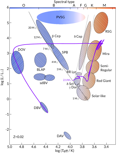
Figure 1: Classes of pulsating variable stars in the Hertzsprung-Russell (HR) diagram, including regions driven by the He II bump ($\delta$ Ceph, $\delta$ Sct, RR Lyrae) and Fe bump ($\beta$ Ceph, SPB) in the opacity. Backslash (\) fills represent pressure modes and slash (/) fills represent gravity modes. The zero age main-sequence (ZAMS, black dashed curve) is labeled with the locations of selected masses. The classical instability strip for radial pulsations is shown by the gray dashed curves. Evolution of a 2.1 $\mathrm{M}_{\odot}$ MESA model (at $Z=0.02$) from ZAMS to a white dwarf (WD) is shown by the purple curve. Figure design from Papics (2013).

Millions of variable stars have been discovered in the Milky Way and Magellanic Clouds, the Local Group (e.g., Optical Gravitational Lensing Experiment, OGLE, Udalski et al. 2015; MACHO Project, Alcock et al. 2003; Palomar Transient Factory, Soraisam et al. 2018) and beyond (e.g., Conroy et al., 2018). Figure 1 shows the broad classifications of these pulsating stars. Pulsating stars such as RR Lyrae and the brighter $\delta$ Cephei (the classical Cepheids) are common, and a strong direct relationship between their luminosities and pulsation periods established Cepheids (Leavitt, 1908; Freedman et al., 2001; Majaess et al., 2009; Riess et al., 2016, 2018) and RR Lyrae in infrared bands (Clementini et al., 2001; Benedict et al., 2002; Klein et al., 2014; Muraveva et al., 2018a, b) as key distance indicators. New classes of variable stars are still being discovered: Blue Large-Amplitude Pulsators (BLAPs) are a new family of pulsating variable stars (Pietrukowicz et al., 2017). BLAPs are rare; only 14 variable stars are attributed by OGLE to this class after examining $\simeq$ 10⁹ stars. They vary in brightness by $\simeq$ 20% on $\simeq$ 30 min timescales (Pietrukowicz et al., 2013). An important new addition to MESA is the capability to model radially-pulsating variable stars.

Numerical energy conservation is rarely discussed by stellar evolution software instrument papers, or shown in science papers as part of establishing robustness of the solutions obtained with the software instrument. Yet stellar evolution calculations generally use low-order, implicit time integration with potentially poorly conditioned matrices whose matrix elements contain limited-precision partial derivatives that can severely limit the quality of solutions. The cumulative effect of such errors can be substantial (Reiter et al., 1995). We implement a set of changes in MESA which, when applicable, can significantly improve the energy conservation properties of stellar evolution models at both global and local levels. This can reduce cumulative errors in energy conservation to 1% or less for applications such as the evolution of a 1 $\mathrm{M}_{\odot}$ model from the pre-main sequence to the end of core He-burning or a core-collapse supernova from soon after explosion to shock breakout.

Rotation modifies a star’s structure (von Zeipel, 1924a; Tassoul, 2000; Maeder & Meynet, 2000). We present a new approach in MESA for calculating the factors that modify the pressure and temperature equations of stellar structure within the shellular approximation. A rotating star is also oblate, with a larger radius at its equator than at its poles. As a result, the equator has a lower surface gravity and thus a lower effective temperature $T_{\rm eff}$ (von Zeipel, 1924b; Chandrasekhar, 1933). Hence, the equator is “gravity darkened”, the poles “gravity brightened”, and this effect can play an important role in the classification of stars. The new extensions to MESA open a pathway for correcting $T_{\rm eff}$ and $L$ for aspect-dependent effects.

Stars transport energy by convection, whether within a core, an envelope, or throughout the interior. These convection regions showcase the interplay between composition mixing, gradients, and diffusion, and the transport of energy through the radial exchange of matter. It is necessary to ensure that convective boundaries are properly positioned because their placement can strongly influence the evolution of the stellar model (Gabriel et al., 2014; Salaris & Cassisi, 2017, Paper IV). We implement an improved algorithm for correctly locating the convective boundaries and naturally allowing the emergence of adiabatic semiconvection regions during core H and He burning.

The paper is organized as follows. Section 2 introduces a new capability to model large-amplitude radially-pulsating variable stars. Section 3 highlights energy conservation in MESA. Section 4 describes new rotation and gravity darkening factors, Section 5 explores a new treatment of convective boundaries, and Section 6 examines the parallel performance of MESAstar. Appendix A reports updates to the equation of state (EOS) and nuclear reaction modules. Appendix B details properties of the rotation factors. Appendix C discusses the current treatment of fallback in core-collapse supernovae (SN), and the thermodynamic evolution from massive star explosions. Appendix D introduces the MESA Testhub for source code development.

Important symbols are defined in Table 1. Acronyms are defined in Table 2. Components of MESA, such as modules and routines, are in typewriter font e.g., eos.

Table 1: Important symbols. Single character symbols are listed first, symbols with modifiers are listed second, and symbols for the RSP convection model are listed third. Some symbols may be further subscripted, for example, by $\mathrm{c}$ (indicating a central quantity), by a cell index $k$, or by species index $i$.

Name	Description	Appears
$\mathcal{A}$	$4\pi r^{2}$   Area of face	2.1
$e$	Specific internal energy	2.1
$E$	Energy	3
$F$	Flux	2.1
$L$	Luminosity	1
$m$	Mass coordinate	2.1
$M$	Stellar mass	1
$\Phi$	Roche potential	4
$p$	Pressure	2.1
$P$	Period	2.1
$\rho$	Mass density	2.1
$r$	Radial coordinate	2.1
$s$	Specific entropy	A.1
$T$	Temperature	2.2
$u$	Velocity	2.1
$V$	1/$\rho$   Specific volume	2.1
$\Omega$	Rotation angular frequency	4
$X$	Hydrogen mass fraction	2.2
$Y$	Helium mass fraction	5
$Z$	Metal mass fraction	2.2
$c_{p}$	Specific heat at constant pressure	1
$c_{V}$	Specific heat at constant volume	A.1
$\delta t$	Numerical time step	3.3
$dm$	Mass of cell	3
$\nabla_{{\rm ad}}$	Adiabatic temperature gradient	3.3
$\nabla_{{\rm L}}$	Ledoux temperature gradient	5
$\nabla_{{\rm rad}}$	Radiative temperature gradient	5
$i_{\rm rot}$	Specific moment of inertia	4
$j_{\rm rot}$	Specific angular momentum	4
$T_{\rm eff}$	Effective temperature	1
$\alpha$	Mixing length parameter	2.1
$\alpha_{\rm c}$	Convective flux parameter	2.1
$\alpha_{\rm cut}$	Artificial viscosity parameter	2.1
$\alpha_{\rm d}$	Turbulent dissipation parameter	2.1
$\alpha_{\rm m}$	Eddy-viscous dissipation parameter	2.1
$\alpha_{\rm p}$	Turbulent pressure parameter	2.1
$\alpha_{\rm s}$	Turbulent source parameter	2.1
$\alpha_{\rm t}$	Turbulent flux parameter	2.1
$C$	$S-D-D_{\rm r}$  convective coupling	2.1
$C_{\rm q}$	Artificial viscosity parameter	2.1
$\Delta u$	Change in velocity across a cell	1
$D$	$\alpha_{\rm d}(e_{\rm t}^{3/2}/\alpha H_{\rm p})$  Turbulent dissipation	2.1
$D_{\rm r}$	($4\sigma\gamma_{\rm r}^{2}/\alpha^{2}$) ($T^{3}V^{2}/c_{p}\kappa H_{\rm p}^{2})e_{\rm t}$	2.1
	Radiative cooling
$\epsilon_{\rm q}$	$(4/3)(q/\rho)\left(\partial u/\partial r-u/r\right)^{2}$	2.1
	Viscous energy transfer rate
$e_{\rm t}$	Specific turbulent energy	2.1
$F_{\rm c}$	$\alpha\alpha_{\rm c}\rho Tc_{p}e_{\rm t}^{1/2}Y_{\rm sag}$  Convective flux	2.1
$F_{\rm r}$	$-$$(4acT^{3}/3\kappa\rho)\ \partial T/\partial r$  Radiative flux	2.1
$F_{\rm t}$	$-$$(\alpha\alpha_{\rm t}\rho H_{\rm p}e_{\rm t}^{1/2})\partial e_{\rm t}/\partial r$  Turbulent flux	2.1
$\gamma_{\rm r}$	Radiative cooling parameter	2.1
$H_{\rm p}$	Pressure scale height	1
$\kappa$	Opacity	1
$p_{\rm av}$	$C_{\rm q}p\left[{\rm min}\left(\Delta u/\sqrt{pV}+\alpha_{\rm cut},\,0\right)\right]^{2}$	2.1
	Artificial viscosity pressure
$p_{\rm t}$	$\alpha_{\rm p}\rho e_{\rm t}$  Turbulent pressure	2.1
$q$	$\alpha_{\rm m}\rho\alpha H_{\rm p}e_{\rm t}^{1/2}$  Kinetic  turbulent  viscosity	2.1
$Q$	($\partial V/\partial T)|_{p}$  Thermal expansion coefficient	1
$s$	Specifc entropy	1
$S$	$\alpha\alpha_{\rm s}e_{\rm t}^{1/2}(TpQ/H_{\rm p})Y_{\rm sag}$  Source function	2.1
$U_{\rm q}$	$(1/\rho r^{3})\ \partial/\partial r\left[\frac{4}{3}qr^{3}\left(\partial u/\partial r-u/r\right)\right]$	2.1
	Viscous momentum transfer rate
$Y_{\rm sag}$	$-H_{\rm p}/c_{\rm p}\ \partial s/\partial r$    superadiabatic gradient	1

Table 2: Acronyms used in this paper.

Acronym	Description	Appears
1O	First Overtone	2.2.2
2O	Second Overtone	2.2.2
BEP	Binary Evolution Pulsators	2.4.4
BLAP	Blue Large-Amplitude Pulsators	1
CHeB	Core Helium Burning	5
CPM	Convective Premixing	5
EOS	Equation of State	1
HADS	High Amplitude Delta Scuti	2.4.6
HR	Hertzsprung Russell	1
LNA	Linear Non-Adiabatic	2.2
MLT	Mixing Length Theory	5
MS	Main Sequence	2.4.6
RSP	Radial Stellar Pulsations	2.1
TAMS	Terminal Age Main Sequence	4.1
WD	White Dwarf	1
ZAMS	Zero Age Main Sequence	1

2 Radial Stellar Pulsations

Cepheids, RR Lyrae, and other classes of variable stars are observed to brighten and dim periodically. They can be modeled as radially symmetric, large amplitude, nonlinear oscillations of self-gravitating gas spheres. Software instruments for precision asteroseismology such as GYRE (Townsend & Teitler, 2013; Townsend et al., 2018) model the small amplitude, linear oscillations of stars. Software instruments such as RSP, described below, are necessary to model the time evolution of large amplitude, self-excited, nonlinear pulsations over many cycles to produce luminosity and radial velocity histories that can be compared to observations.

Early nonlinear radial pulsation models considered purely radiative envelopes (e.g., Christy, 1964; Stellingwerf, 1975; Castor et al., 1977; Aikawa & Simon, 1983). Later, radiation hydrodynamic treatments followed with implicit adaptive grids (Dorfi & Drury, 1987; Dorfi & Feuchtinger, 1991). While these purely radiative models qualitatively reproduced light and radial velocity curves, it was clear that convection driven by partial ionization of H and He carries most of the flux in the envelopes of RR Lyrae and Cepheids. Prescriptions for coupling convection with pulsations were developed (e.g., Stellingwerf, 1982; Kuhfuß, 1986) that reside, with modifications, in modern software instruments (Bono & Stellingwerf, 1994; Yecko et al., 1998; Kolláth et al., 2002; Smolec & Moskalik, 2008). Models from these software instruments can reproduce the overall morphology of light and radial velocity curves of classical pulsators (e.g., Feuchtinger et al., 2000; Marconi et al., 2015), features of specific objects (e.g., Keller & Wood, 2006; Marconi et al., 2013; Smolec et al., 2013), and dynamical phenomena such as the Hertzsprung progression (e.g., Hertzsprung, 1926a; Bono et al., 2000). Unsolved problems include double-mode pulsations (Kolláth et al., 2002; Smolec & Moskalik, 2010) and the cyclic modulations of RR Lyrae light curves (e.g., the Blazhko effect, Blažko, 1907; Szabó et al., 2010). For background material we refer the reader to Gautschy & Saio (1995, 1996), Buchler (2009), and Marconi (2017).

2.1 Radial Stellar Pulsations - RSP

RSP is a new functionality in MESAstar that models large amplitude, self-excited, nonlinear pulsations that stars develop when they cross instability domains in the HR diagram (see Figure 1). RSP is closely integrated with the MESA environment. Instead of calling the standard MESAstar routine to evaluate equations and solve for a new model using Newton-Raphson iterations (see Section 3), a separate routine does the same for RSP using a different set of equations and a different Newton-Raphson solver. The different equations include time-dependent convection in a form appropriate for modelling nonlinear pulsations, and the different solver uses a band diagonal matrix approach since the equations as currently implemented do not fit into a three-block stencil needed for the standard block tridiagonal solver. Moreover, instead of calling the usual MESAstar routine to get a starting model, a separate routine creates an RSP model envelope that is consistent with the RSP set of equations. RSP uses the same MESA opacity and equation of state (EOS) modules, inlist structure, profile and history output files, photo files for saving and restarting runs, run_star_extras extensions, and hooks for using externally supplied routines.

RSP follows Smolec & Moskalik (2008), where the momentum and specific internal energy equations are

$$\frac{\mathrm{D}u}{\mathrm{D}t}=-\mathcal{A}\frac{\partial}{\partial m}\left(p+p{\rm{}_{t}}+p_{\rm av}\right)+U_{\rm q}-\frac{Gm}{r^{2}}\,,$$ (1)

$$\frac{\mathrm{D}e}{\mathrm{D}t}+\left(p+p_{\rm av}\right)\frac{\mathrm{D}V}{\mathrm{D}t}=-\frac{\partial}{\partial m}\left[\mathcal{A}\left(F_{\rm r}+F_{\rm c}\right)\right]-C\,,$$ (2)

where $\mathrm{D}/\mathrm{D}t$ is the Lagrangian time derivative. The generation of a specific turbulent energy, $e_{\rm t}$, is described by the one-equation Kuhfuß (1986) model

$$\frac{\mathrm{D}e_{\rm t}}{\mathrm{D}t}+p_{\rm t}\frac{\mathrm{D}V}{\mathrm{D}t}=-\frac{\partial}{\partial m}\left(\mathcal{A}F_{\rm t}\right)+\epsilon_{\rm q}+C\,.$$ (3)

The latter two equations are added to give an equation for the specific internal and turbulent energies

$$\frac{\mathrm{D}}{\mathrm{D}t}\left(e+e_{\rm t}\right)+\left(p+p_{\rm t}+p_{\rm av}\right)\frac{\mathrm{D}V}{\mathrm{D}t}=\\ -\frac{\partial}{\partial m}\left[\mathcal{A}\left(F_{\rm r}+F_{\rm c}+F_{\rm t}\right)\right]+\epsilon_{\rm q}\,.$$ (4)

Definitions for all terms entering these equations are given in Table 1. RSP solves Equations (1), (3), and (4). The diffusion approximation is used for the radiative flux $F_{\rm r}$ and its numerical implementation follows Stellingwerf (1975). Numerical implementation of the superadiabtic gradient follows Stellingwerf (1982). All equations are discretized on a Lagrangian mesh.

Several quantities enter the convection model. For the momentum equation these are the turbulent pressure $p_{\rm t}$ (Table 1 lists the relationship with the specific turbulent energy $e_{\rm t}$) and viscous momentum transfer rate $U_{\rm q}$. For the turbulent energy equation these are the work done by turbulent pressure, the divergence of the turbulent flux $F_{\rm t}$, and the viscous energy transfer rate $\epsilon_{\rm q}$. The convective coupling term $C=S-D-D_{\rm r}$ appears with opposite sign in the internal and turbulent energy equations. Generation of the turbulent energy is driven by the source function $S$, while turbulent dissipation $D$ and radiative cooling $D_{\rm r}$ contribute to its decay. Radiative cooling of convective eddies follows Wuchterl & Feuchtinger (1998). Details of the turbulent convection model are discussed in Kuhfuß (1986), Wuchterl & Feuchtinger (1998) and Smolec & Moskalik (2008).

Table 3: Free parameters of the RSP convection model, their base values, and associated MESA controls that multiply the base values.

Parameter  $=$	Base Value  $\times$	Control Value
$\alpha$	$1$	RSP_alfa
$\alpha_{\rm m}$	$1$	RSP_alfam
$\alpha_{\rm s}$	$(1/2)\sqrt{2/3}$	RSP_alfas
$\alpha_{\rm c}$	$(1/2)\sqrt{2/3}$	RSP_alfac
$\alpha_{\rm d}$	$(8/3)\sqrt{2/3}$	RSP_alfad
$\alpha_{\rm p}$	$2/3$	RSP_alfap
$\alpha_{\rm t}$	$1$	RSP_alfat
$\gamma_{\rm r}$	$2\sqrt{3}$	RSP_gammar

These terms in the convection model depend on the free parameters listed in Table 3. If radiative cooling and turbulent pressure are neglected, the time-independent version of the Kuhfuß (1986) convection model reduces to standard mixing length theory provided base values are used for $\alpha_{\rm s}$, $\alpha_{\rm c}$ and $\alpha_{\rm d}$ (associated controls set to 1). Base values for $\alpha_{\rm p}$ and $\gamma_{\rm r}$ follow Yecko et al. (1998) and Wuchterl & Feuchtinger (1998), respectively. Experience suggests $\alpha_{\rm t}\simeq 0.01$, $\alpha_{\rm m}\lesssim 1$, and $\alpha\lesssim 2$ are useful starting choices.

Periods of pulsation modes depend weakly on the values of these free parameters. Pulsation growth rates and light and radial velocity curves are, however, sensitive to the free parameters. Calibration with multiple observational constraints is unlikely to yield a unique set of parameters that gives satisfactory results across the HR diagram for all pulsation modes. We stress that parameter surveys are an essential part of any science application of RSP.

In Equations (1) and (2), $p_{\rm av}$ is the artificial viscosity pressure (Richtmyer, 1957) for numerically handling shocks that may develop during pulsations. We adopt the Stellingwerf (1975) two-parameter formulation as the default. The Tscharnuter & Winkler (1979) artificial pressure-tensor form, which was implemented in Paper III, can also be used in RSP.

The numerical scheme to solve discrete versions of the equations is based on the intrinsically energy conserving method given by Fraley (1968). Details of the numerical implementation, along with RSP’s lineage (Stellingwerf, 1975; Kovacs & Buchler, 1988), are discussed in Smolec & Moskalik (2008). During the nonlinear integration, $u=0$, $L={\rm constant}$ and $e_{t}=0$ at the inner boundary (See Figure 2). The latter condition holds also for the outermost boundary, i.e., outermost cell is radiative. External pressure is fixed and zero by default.

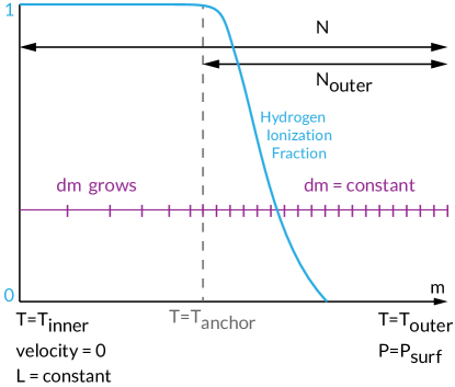
Figure 2: Grid structure in RSP. The inner boundary at the base of the static envelope is defined by a chosen temperature (RSP_T_inner). The model surface has a fixed temperature $T_{\rm outer}$, derived from $T_{\rm eff}$, and pressure (RSP_Psurf). The anchor temperature (RSP_T_anchor) is usually located where H ionizes, shown by the blue curve. The envelope is divided into $N$ Lagrangian mass cells (RSP_nz). Between the anchor and the surface are $N_{\rm outer}$ cells (RSP_nz_outer), each with a constant mass. Between the inner boundary and the anchor the mass of each cell increases.

2.2 RSP in Action

RSP performs three operations: building an initial model; conducting a linear non-adiabatic (LNA) stability analysis on that model; and integrating the time-dependent nonlinear equations.

2.2.1 Building an Initial Model

Since the energy density of radial pulsations drops rapidly going inward from a star’s surface, a full stellar model reaching to the center is frequently not necessary. The use of RSP is currently restricted to cases in which pulsations are determined by the structure of the envelope and are independent of the detailed structure of the core. RSP begins by building a chemically homogeneous envelope from given stellar parameters ($M$, $L$, $T_{\rm eff}$, $X$, and $Z$). These parameters can be freely chosen and need not originate from a MESAstar model. It is not yet possible to directly import an envelope from MESAstar into RSP  primarily because of the different treatments of convection (a version of mixing length theory in MESAstar versus detailed time evolution of turbulence in RSP). Tighter integration of MESAstar and RSP is a future project.

Specifications for the initial model include the number of cells and the temperature at the base (see Figure 2). This inner boundary temperature is defined by a chosen temperature (RSP_T_inner $\simeq$ 2$\times$10⁶ $\mathrm{K}$) that should be set hot enough so that the eigenvector amplitudes generated in the following stability analysis go to zero, and cool enough to exclude regions of nuclear burning and justify the assumption of chemical homogenity. The model is divided into inner and outer regions at a specified anchor temperature. In the outer region, cells have the same mass; in the inner region cell masses grow by a constant factor so that the innermost cells are significantly larger than the ones at the surface. The anchor temperature should be in the part of the model driving the pulsations. For example, for pulsations in the classical instability strip a value of $T_{\rm anchor}$=11,000 $\mathrm{K}$ is typical. In the case of $Z$-bump pulsations a higher temperature would be appropriate. Proper choice of the number of outer cells and placement of the anchor are necessary to ensure that the driving region is well resolved.

The initial model builder iteratively constructs an envelope in hydrostatic equilibrium that satisfies the RSP equations. Starting from the outer radius determined by $L$ and $T_{\rm eff}$ this process involves selection of a cell mass to be used in the outer part of the envelope and a scale factor that is used to progressively increase cell masses in the inner region. Those choices must match the desired number of cells, both $N$ and $N_{\rm outer}$, and also satisfy the surface boundary conditions and the required temperatures at the anchor location and at the inner boundary. The model builder is a complex multistage iterative procedure that works well for the range of cases presented in the following but may fail when applied outside of that range.

2.2.2 Stability Analysis

The LNA analysis is performed on the initial model using a full linearization of the RSP equations (for details see Smolec, 2009). These include time-dependent convection, moving beyond the frozen-in convection approximation made in software instruments like GYRE. This yields the eigenmodes, periods, and growth rates. The eigenvectors are used to perturb the initial model for the time evolution.

Figure 3 shows amplitudes of radial displacements and differential work for the first three eigenmodes of the classical Cepheid model in the MESA test_suite. A common resolution for exploratory model surveys, $N=150$ and $N_{\rm outer}=40$, is adopted. For $T\gtrsim 5\times 10^{5}\,\mathrm{K}$, the displacements and differential work of all three radial eigenmodes are negligible, indicating that the extent of the computational domain is sufficient.

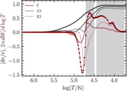
Figure 3: RSP LNA analysis of a classical Cepheid model. Shown are the displacement amplitudes (black) and the differential work (red) done by the lowest three radial eigenmodes. The thickest curves are for the fundamental (F) mode, medium thickness for the first overtone (1O) mode and the thinnest curves for the second overtone (2O) mode. The dots indicate the cell locations. The grey areas show the extent of the convection zones around H ionization, first He and second He ionization, respectively.

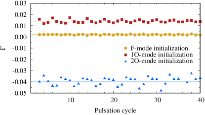
Figure 4: Comparison of the fractional growth rate $\Gamma$ during the initial cycles of the time integration. Horizontal lines show the LNA predictions. An RR Lyrae model ($M$ = 0.65 $\mathrm{M}_{\odot}$, $L$ = 45 $\mathrm{L}_{\odot}$, $T_{\rm eff}$ = 7,100 $\mathrm{K}$, $X$ = 0.75, $Z$ = 0.0014) was initialized with a 0.1 $\mathrm{km}\,\mathrm{s}^{-1}$ amplitude pure F-mode (circles), 1O-mode (squares), or 2O-mode (triangles) and evolved.

2.2.3 Evolution in the Linear Regime

The initial static model is perturbed with a linear combination of the velocity eigenvectors of the three lowest order radial modes. More specifically, the velocity eigenvectors are scaled to have a surface value of 1. RSP_fraction_1st_overtone and RSP_fraction_2nd_overtone multiply the 1O and 2O eigenvectors, respectively. The F-mode eigenvector is then multiplied by (1 - RSP_fraction_1st_overtone - RSP_fraction_2nd_overtone). The linear combination of these three scaled eigenvectors is then multiplied by the surface velocity RSP_kick_vsurf_km_per_sec.

The time integration commences with a constant time step (RSP_target_steps_per_cycle) and continues for a specified number of pulsation cycles (RSP_max_num_periods). A new cycle begins when the model passes through a maximum radius. Controls allow filtering out secondary maxima in the radial velocity curve.

Figure 4 shows $\Gamma$ the fractional growth of the kinetic energy per pulsation period near the start of a time integration, where

$$\Gamma=2(E_{\rm k,\,max}^{i+1}-E_{\rm k,\,max}^{i})/(E_{\rm k,\,max}^{i+1}+E_{\rm k,\,max}^{i}),$$ (5)

and $E_{\rm k,\,max}^{i}$ is the maximum kinetic energy of the envelope during pulsation cycle $i$. Agreement between these three time integrations and the corresponding LNA analyses is satisfactory. Similarly, the pulsation periods match the linear values during the low-amplitude phase of development. Consistency between the time integrations and LNA analyses form the basis for interpreting the nonlinear results.

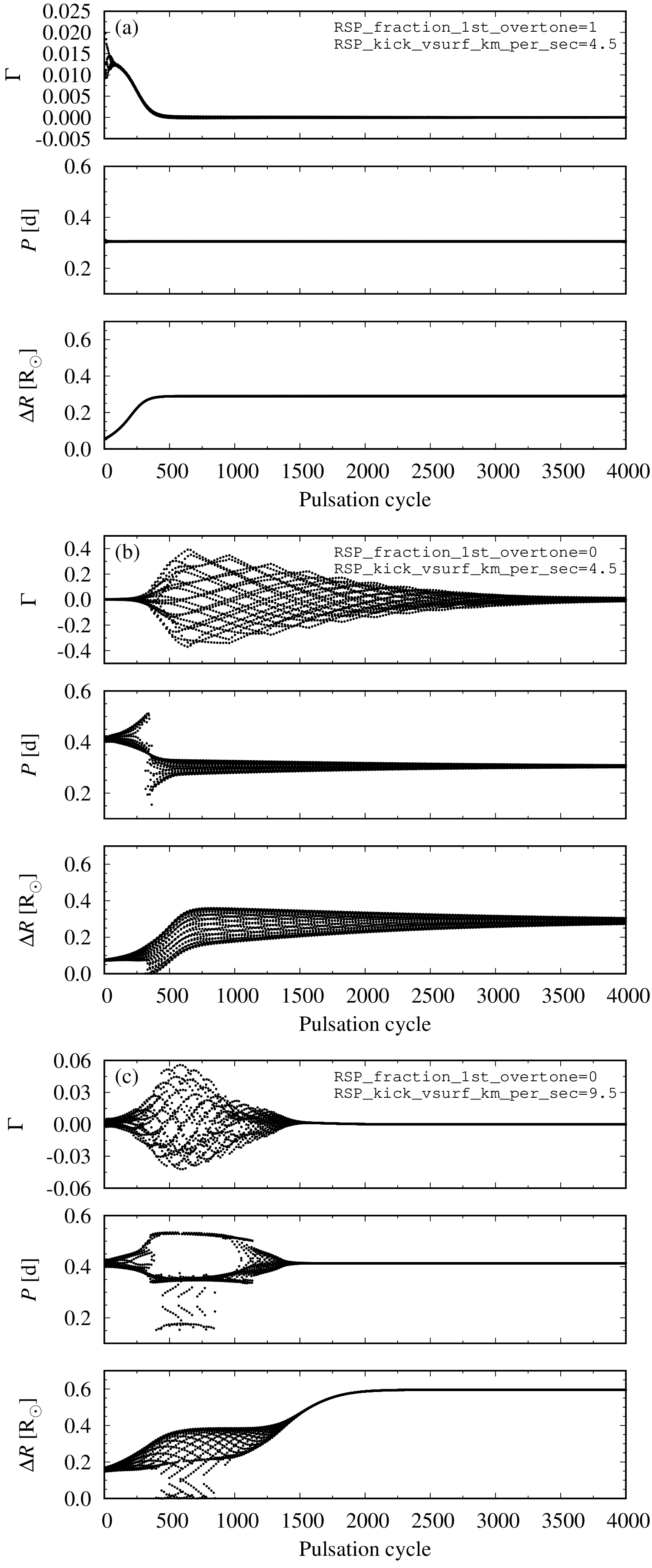
Figure 5: Fractional growth rate $\Gamma$, period $P$, and amplitude of radius variation $\Delta R$ during 4,000-cycle integrations of the same RR Lyrae model as in Figure 4 with three different initial conditions labelled (a), (b), and (c).

2.2.4 Different Perturbations, Different Periods

Which of the perturbed modes attains large-amplitude pulsations in the nonlinear regime may depend on the initial conditions (e.g., Smolec, 2014). Figure 5 shows the results of longer time integrations for the RR Lyrae model shown in Figure 4. The upper triplet of panels, case (a), is for a 1O-mode initialization with a 4.5 $\mathrm{km}\,\mathrm{s}^{-1}$ amplitude. The middle triplet panel, case (b), is for a F-mode initialization with 4.5 $\mathrm{km}\,\mathrm{s}^{-1}$ amplitude. The lower triplet, case (c), is for an F-mode initialization with a 9.5 $\mathrm{km}\,\mathrm{s}^{-1}$ amplitude.

For case (a), the pulsations converge towards a single, 1O-mode pulsation. After a $\simeq$ 500 cycle transient phase the pulsation period and radius amplitude barely change and $\Gamma\simeq 0$. For case (b), the model has not converged to a single-periodic mode after $4,000$ cycles. Despite the pure F-mode initialization, at $\simeq$ 300 cycles the pulsation switches toward the 1O mode. This does not prove the model cannot pulsate in the F-mode, as case (c) demonstrates. After a transient phase with beating F and 1O modes, the 1O mode decays and the single-periodic F-mode pulsation grows to saturation.

Figure 5 is an example of two different single-mode solutions whose selection depends on the initial conditions. Two stars can have the same physical parameters but pulsate in different modes depending on their evolutionary history.

Table 4: Convective parameter sets referred to in the text as A, B, C, or D. Note that the controls multiply base values (see Table 3).

Control	Set A	Set B	Set C	Set D
RSP_alfa	1.5	1.5	1.5	1.5
RSP_alfam	0.25	0.50	0.40	0.70
RSP_alfas	1.0	1.0	1.0	1.0
RSP_alfac	1.0	1.0	1.0	1.0
RSP_alfad	1.0	1.0	1.0	1.0
RSP_alfap	0.0	0.0	1.0	1.0
RSP_alfat	0.00	0.00	0.01	0.01
RSP_gammar	0.0	1.0	0.0	1.0

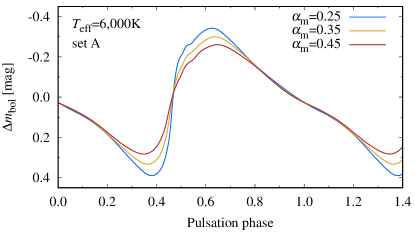
Figure 6: Bolometric light curve of the $T_{\rm eff}$=6,000 $\mathrm{K}$ Cepheid model of with convective parameters of set A but with varying eddy-viscous dissipation $\alpha_{\rm m}$.

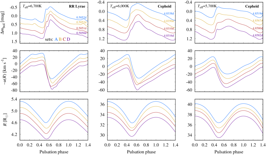
Figure 7: Bolometric light (upper panel), radial velocity (middle panel) and radius curves (lower panel) for an RR Lyrae F-mode model (left; $M$ = 0.65 $\mathrm{M}_{\odot}$, $L$ = 45 $\mathrm{L}_{\odot}$, $T_{\rm eff}$ = 6,700 $\mathrm{K}$, $X$ = 0.75, $Z$ = 0.0014) and two F-mode classical Cepheid models ($M$ = 4.15 $\mathrm{M}_{\odot}$, $L$ = 1,400 $\mathrm{L}_{\odot}$, $X$ = 0.73, $Z$ = 0.007) at $T_{\rm eff}$=6,000 $\mathrm{K}$ (middle panel) and $T_{\rm eff}$=5,700 $\mathrm{K}$ (right panel). The mass and luminosity for the Cepheid models are close to the values derived for OGLE-LMC-CEP-227 (Pilecki et al., 2018). Each curve corresponds to a set of convective parameter values listed in Table 4. The mean magnitude of the bolometric light curves is set to zero. Light curves are vertically offset by 0.3 mag, radial velocity curves by $10\,\mathrm{km}\,\mathrm{s}^{-1}$ and radius curves by $0.2\,\mathrm{R}_{\odot}$ (RR Lyrae) or $1\,\mathrm{R}_{\odot}$ (Cepheids).

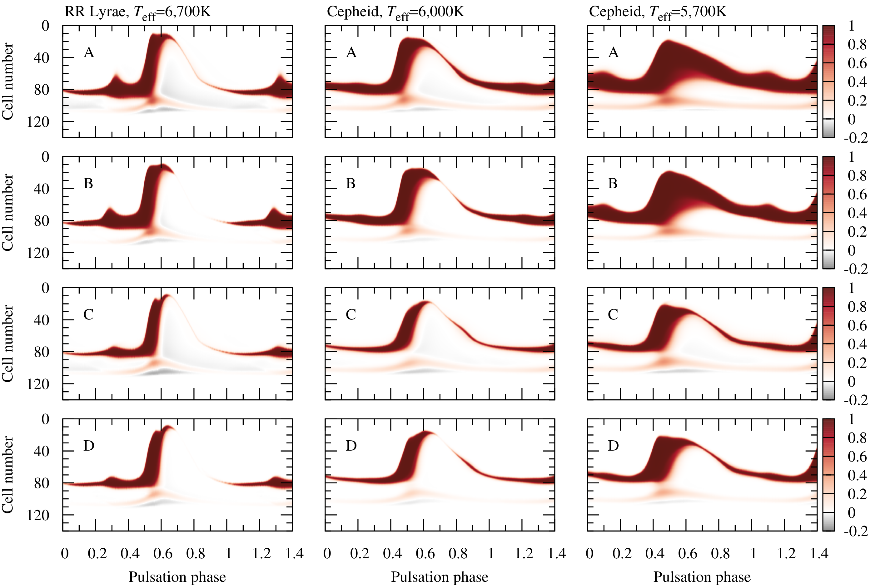
Figure 8: Evolution of convective luminosity $L_{\rm c}/L$ for the models shown in Figure 7. Cell number on the y-axis serves as a spatial coordinate, with cell 0 marking the stellar surface. The radiative interior of each model is not shown.

2.2.5 Convection Parameter Sensitivity

The final state in the nonlinear regime is usually a single-periodic oscillation. The shape of the light and radial velocity curves may depend on the values of the eight free parameters listed in Table 3. In Table 4 set A corresponds to the simplest convection model. Set B adds radiative cooling, set C adds turbulent pressure and turbulent flux, and set D includes these effects simultaneously. The parameter $\alpha_{\rm m}$ has little effect on the shape of the light curve but strongly affects its amplitude. Figure 6 shows the effect of varying $\alpha_{\rm m}$ on the $T_{\rm eff}$=6,000 $\mathrm{K}$ Cepheid model. The free parameter $\alpha_{\rm m}$ may thus be used to match the observed amplitude. For sets A-D, $\alpha_{\rm m}$ was adjusted so that models with different sets have similar amplitudes.

Figure 7 shows the effect of these parameter sets on the shapes of the bolometric light, photosphere radial velocity, and radius variation curves for a saturated F-mode RR Lyrae and two saturated F-mode classical Cepheid models. The pulsation periods, radial velocity curves, and radius variation curves show only small differences. For the RR Lyrae models, there are differences in the fine structure of the light curves. For example, the bump before minimum light is weaker when turbulent pressure and turbulent flux are included (sets C and D). The shape of the light curve near maximum light also differs for both the RR Lyrae and Cepheid models.

Figure 8 shows the convective luminosity profiles for the models of Figure 7. Depending on pulsation phase, one convective region (darker hues) extends from the surface cells down to cell $\simeq$ 90. This convective region is associated with partial ionization of H and He. Another convective region (lighter hues) lies deeper in the envelope, centered at cell $\simeq$ 110, and is associated with the second ionization of He. In most of the models these two convective regions merge at pulsation phase $\simeq\,$0.5 during maximum contraction when both convective regions are at their strongest and most extended. In the cooler models, the first convective region carries nearly all of the luminosity throughout a pulsation cycle. In the hotter models, this convective region becomes very weak at pulsation phase $\simeq$ 0.8 (before maximum expansion) and is barely resolved as it progresses deeper into the envelope. This behavior is pronounced in the RR Lyrae models with radiative cooling (sets B and D), as cooling contributes to damping the turbulent energy and hence the near disappearance of the convective region.

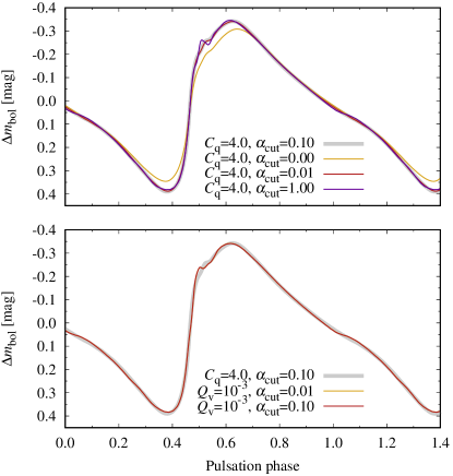
Figure 9: Sensitivity of the bolometric light curve shape of Cepheid model on artificial viscosity: $\alpha_{\rm cut}$ (upper panel) in the Stellingwerf (1975) formulation, and $\alpha_{\rm cut}$ in the Tscharnuter & Winkler (1979) formulation (lower panel). The light curve with $C_{\rm q}$=4.0 and $\alpha_{\rm cut}$=0.1 is shown as a gray curve.

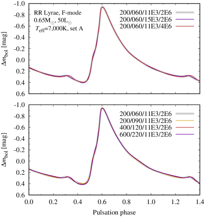
Figure 10: Sensitivity of the bolometric light curve of an F-mode RR Lyrae model to the grid, labeled as $N/N_{\rm outer}/T_{\rm anchor}/T_{\rm inner}$. The light curve for the default grid is shown by the gray curve. The upper panel shows the effects of different $T_{\rm anchor}$/$T_{\rm inner}$. The lower panel shows the effects of different $N/N_{\rm outer}$ combinations.

2.2.6 Artificial Viscosity Sensitivity

There are two parameters, $\alpha_{\rm cut}$ and $C_{\rm q}$, that control the Stellingwerf (1975) artificial viscosity, entering into the definition of $p_{\rm av}$ (see Table 1). Figure 9 shows the effect of these parameters on light curves for the $T_{\rm eff}$ = 6,000 $\mathrm{K}$ Cepheid model. The value of $C_{\rm q}$ plays a minor role. For $C_{\rm q}=4$, the upper panel shows a different light curve develops only if $\alpha_{\rm cut}$ = 0.0, corresponding to artificial viscosity acting for very small compressions, which leads to excessive dissipation that quenches the pulsation amplitude. For $\alpha_{\rm cut}$ $\geq$ 0.01, the light curves are similar and roughly have the same pulsation amplitude. When $\alpha_{\rm cut}$ = 0.1, artificial viscosity turns on only for strong shocks, seen as the wiggle on the ascending branch of the light curve. This choice ($\alpha_{\rm cut}$ = 0.1) numerically captures shocks without excessive dissipation, barely affecting the light curve shape and amplitude. While an artificial viscosity modifies the velocity structure in the envelope at each epoch, we find that these differences are smaller than the differences for the bolometric light curves. The lower panel shows that the Tscharnuter & Winkler (1979) form of artificial viscosity yields light curves with the same amplitude and qualitatively the same shape. Small differences are apparent at a shock-prone phase shortly before the maximum brightness.

2.2.7 Spatial and Temporal Sensitivity

Figure 10 shows the sensitivity of the bolometric light curve to the total number of cells $N$, number of cells above the anchor $N_{\rm outer}$, anchor location $T_{\rm anchor}$, and inner boundary location $T_{\rm inner}$ for an RR Lyrae model ($M$ = 0.65 $\mathrm{M}_{\odot}$, $L$ = 50 $\mathrm{L}_{\odot}$, $T_{\rm eff}$ = 7,000 $\mathrm{K}$, $X$ = 0.75, $Z$ = 0.0014) with convective parameter set A.

For classical pulsators, $T_{\rm inner}$ is typically placed at 2$\times$10⁶ $\mathrm{K}$, and common choices for $T_{\rm anchor}$ are 11,000 $\mathrm{K}$ or 15,000 $\mathrm{K}$. The upper panel shows that the light curves are weakly sensitive to the choice of $T_{\rm inner}$ and $T_{\rm anchor}$ for this RR Lyrae model. Light and radial velocity curves are usually the most sensitive to $N$ and $N_{\rm outer}$. The lower panel shows this effect is small for this RR Lyrae model. Section 2.4.4 shows a case with a much larger sensitivity.

The default value of 600 time steps per pulsation cycle works well for most cases, but smaller time steps are recommended for models that include radiative cooling, turbulent pressure, turbulent flux, or develop violent pulsations (e.g., the chaotic models of Section 2.4.3). We stress that there is no unique choice of grid or time step that will work for all applications or guarantees convergence. All nonlinear modeling of variable stars should be accompanied by sensitivity and convergence tests.

2.3 Current Limitations and Plans for the Future

RSP in its present form covers most of the classical instability strip including $\delta$ Cepheids, RR Lyrae, High Amplitude $\delta$ Scuti and SX Phoenicis stars (see Figure 1), where a single or just a few dominant radial modes are observed. RSP also has applications outside of the classical instability strip as we show below for BLAPs. For stars close to the main sequence, linear growth rates are very small and thus, as we show below, long time integrations are necessary to approach full-amplitude nonlinear pulsations.

RSP is currently of limited use for strongly non-adiabatic pulsations with large $L/M$ ratios, including Luminous Blue Variables, Mira-type variables, and type II Cepheids. For the latter, only the shortest-period BL Her class variables can be reliably modeled (see Section 2.4.3). For the longer-period classes of W Vir and RV Tau variables, either static envelopes cannot be constructed or nonlinear integrations break down at the onset due to violent relaxations of the outermost layers. In the extended envelopes of these variable stars the radiation-diffusion approximation is inadequate due to the low optical depth. The inclusion of pulsation-driven mass loss may also be necessary to study pulsations of these variable stars (Smolec, 2016).

Inclusion of turbulent pressure and flux may lead to convergence difficulties when constructing the static initial envelope. Cooler stellar envelopes with higher Mach number convection are also numerically more difficult than hotter envelope models. These difficulties are rooted in the static grid structure shown in Figure 2. Future developments of RSP should include a more versatile initial model builder, adaptive remeshing during the time integration, and a radiation-hydrodynamic treatment of the radiative energy and flux.

2.4 Applications of RSP

We now apply RSP to variable stars. Examples include the light curves of classical pulsators, modeling of specific objects, and models for the dynamics of modulated or chaotic pulsations.

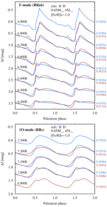
Figure 11: $I$-band light curves of F-mode (upper panel) and 1O-mode (lower panel) pulsators across the instability strip for $M$ = 0.65 $\mathrm{M}_{\odot}$, $L$ = 45 $\mathrm{L}_{\odot}$, [Fe/H] = $-$1.0, and convective sets B (blue) and D (red). Light curves are labelled with their $T_{\rm eff}$  and period, and offset vertically to facilitate comparisons (by 0.5 in the upper panel and 0.4 in the lower panel).

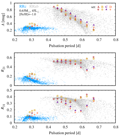
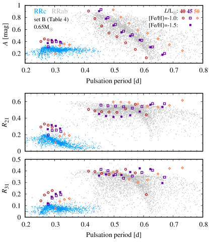
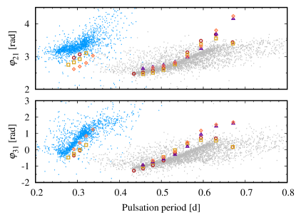
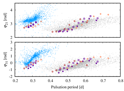
Figure 12: Comparison of the peak-to-peak amplitude and low-order Fourier decomposition parameters of $I$-band light curves of Galactic bulge RRab stars (gray dots) and RRc stars (blue dots) with synthetic light curves (symbols). In the left panels physical parameters are fixed, except for $T_{\rm eff}$ and different convective parameter sets. In the right panels, the convective model is fixed and physical parameters are varied. Observational data are from Soszyński et al. (2014).

2.4.1 RR Lyrae variables

We consider two sequences of RR Lyrae-type models. The first sequence has $M$ = 0.65 $\mathrm{M}_{\odot}$, $L$ = 45 $\mathrm{L}_{\odot}$ and [Fe/H] = $-$1.0 ($X$ = 0.75, $Z$ = 0.0014) with $T_{\rm eff}$ varying in 100 $\mathrm{K}$ steps for convective sets A–D. Figure 11 shows a gallery of $I$-band light curves from this sequence. The upper panel shows F-mode pulsators (commonly known as RRab stars) and the lower panel shows 1O-mode pulsators (known as RRc stars). The latter have smaller amplitudes and are less nonlinear in shape (i.e., more sinusoidal) than the F-mode light curves. Models with different convective settings differ the most near minimum and maximum light. For example, F-mode models with convective set B develop a bump preceding minimum light that is absent in the light curves with convective set D. On the other hand, F-mode models with cooler $T_{\rm eff}$ from convective set D develop broad, double-peaked light curve maxima that are absent in models from convective set B.

To compare the overall morphology of $I$-band light curves from these sequences with OGLE observations, we perform a Fourier decomposition of the synthetic light curves

$$I(t)=A_{0}+\sum_{k}A_{k}\sin(2\pi kft+\phi_{k})\,,$$ (6)

where $f$ is the pulsation frequency, and $A_{k}$ and $\phi_{k}$ are amplitudes and phases, respectively. We then construct the amplitude ratios $R_{k1}$ and epoch-independent phase differences $\varphi_{k1}$ (Simon & Lee, 1981):

$$R_{k1}=\frac{A_{k}}{A_{1}}\,,\quad\varphi_{k1}=\phi_{k}-k\phi_{1}\,.$$ (7)

Observationally derived values of $R_{k1}$ and $\varphi_{k1}$ are taken from the OGLE catalog (Soszyński et al., 2014) and shown in Figure 12 by gray dots for RRab (F-mode) stars and blue dots for RRc (1O-mode) stars. The observations show that the Fourier parameters follow progressions with pulsation period, traced by the highest density of data points, but with significant scatter. Fourier parameters from the model $I$-band light curves are shown with colored symbols. Left panels are for the first sequence of models. Right panels are for the second sequence, which has $M$ = 0.65 $\mathrm{M}_{\odot}$, convective set B, $T_{\rm eff}$ varying in $100\,\mathrm{K}$ steps, and either $L$ = (40, 45, 50)$\mathrm{L}_{\odot}$  at [Fe/H] = $-$1.0 or $L$ = 45 $\mathrm{L}_{\odot}$ at [Fe/H] = $-$1.5.

The left panels show that F-mode pulsators with convective sets A and B progress similarly. Models with convective sets C and D also progress similarly but are qualitatively different than those with convective sets A and B. These differences are more pronounced for cooler, longer period, models. The overall match of the F-mode decompositions with the OGLE RRab stars (gray points) is reasonable but shows some systematic differences. For example, the model values of $\varphi_{31}$ are larger than the observed values. However, the model physical parameters except $T_{\rm eff}$ are fixed, while this is not the case for the OGLE RRab stars.

The match between the 1O-mode models and the OGLE RRc stars (blue points) is worse. The amplitudes and the amplitude ratios are systematically too large. The Fourier phases are systematically too small. This may indicate different convective parameters are needed to reproduce the observed light curve shapes of F-mode and 1O-mode pulsators. Note the 1O-mode instability strip with convective set C is smaller than the F-mode instability strip at the luminosity considered. Models from set C, where the 1O-mode is linearly unstable and the integration is initialized with a 1O-mode velocity perturbation, all switch to an F-mode pulsation.

The right panels in Figure 12 show that the light curve shapes are sensitive to the physical parameters. By varying the luminosity and metallicity in a narrow range, the model sequences match the OGLE values. However, no sequence considered follows the OGLE progression, because RR Lyrae in the Galactic bulge are characterized by mass, luminosity and metallicity distributions that cannot be reproduced with a single sequence.

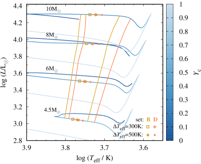
Figure 13: Evolutionary tracks in the HR diagram, shaded to show the core He mass fraction, $Y_{\rm c}$. Blue and red edges of the instability strip for convective sets B and D are shown, along with the locations where non-linear Cepheid models are computed (symbols).

2.4.2 Classical F-mode Cepheids

Cepheids display a feature known as the Hertzsprung progression (Hertzsprung, 1926b). A secondary bump in their light and radial velocity curves appears near minimum light on the descending branch when $P$ $\simeq$ 5 d. The bump moves towards earlier phases on the descending branch as the period increases and is coincident with maximum light when $P$ $\simeq$ 10 d. The bump then moves onto the ascending branch for longer periods and disappears at $P$ $\simeq$ 20 d. The bump is driven by a 2:1 resonance between the F-mode and a damped 2O-mode (e.g., Simon & Schmidt, 1976; Buchler et al., 1990). This behavior is reflected in Cepheids’ Fourier parameters, which follow more complex progressions with pulsation period than the RR Lyrae stars.

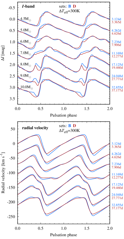
Figure 14: $I$-band light curves (upper panel) and radial velocity curves (lower panel) for the Cepheid models with a $\Delta$$T_{\rm eff}$ = 300 $\mathrm{K}$ offset from the blue edge and convective sets B and D. Light curves are labelled with their pulsation periods and offset vertically by 0.5 mag or 35 $\mathrm{km}\,\mathrm{s}^{-1}$ to facilitate comparison. Radial velocity curves follow the same order.

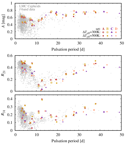
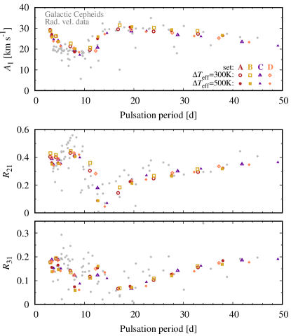
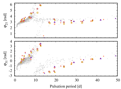
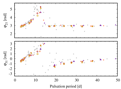
Figure 15: Amplitudes and Fourier parameters for $I$-band light curves (left panel) and radial velocity curves (right panel). Observations are marked with gray dots. Light curve data are from Soszyński et al. (2015) and Ulaczyk et al. (2013) and radial velocity curve data are from Storm et al. (2011). For the light curves the peak-to-peak amplitude is shown, while for radial velocity curves the Fourier amplitude is scaled with a $p$-factor of 1.3. Models are plotted with colored symbols.

We consider 4.5, 5.0, 6.0, 7.0, 8.0, 9.0, and 10.0 $\mathrm{M}_{\odot}$ models with $X$ = 0.736, $Z$ = 0.008 and convective parameter sets A–D. Further details are in the test suite example 5M_cepheid_blue_loop. Figure 13 shows the evolutionary tracks during the core He burning, blue-loop phase for a selection of masses. Blue and red edges of the instability strip computed with RSP for convective sets B and D are shown. Edges for convective sets A and C largely overlap those for convective sets B and D, respectively. Nonlinear pulsation models are computed with a $\Delta$$T_{\rm eff}$ = 300 $\mathrm{K}$ or 500 $\mathrm{K}$ offset from the blue edge.

Figure 14 shows $I$-band light curves and radial velocity curves for the $\Delta$$T_{\rm eff}$ = 300 $\mathrm{K}$ models. Due to the shift in the location of blue edge models, models from convective sets B and D have different $T_{\rm eff}$ and consequently different pulsation periods. Figure 15 compares Fourier parameters of the Cepheid models with those derived from LMC Cepheid light curves (left panel, Soszyński et al., 2015; Ulaczyk et al., 2013) and Galactic F-mode Cepheid radial velocity curves (right panel, Storm et al., 2011). The $I$-band light curves are more sensitive to the convective parameters than the radial velocity curves for both $\Delta$$T_{\rm eff}$ offsets. As with the RR Lyrae models, the Fourier parameters for convective sets A and B are similar to each other, as are those for sets C and D. The radial velocity Fourier parameters follow tighter progressions than the $I$-band light curves.

The Fourier phases in the left panels of Figure 15 are systematically larger than the observationally-inferred values for $P\lesssim 10$ d, with the difference being larger for the cooler $\Delta$$T_{\rm eff}$ = 500 $\mathrm{K}$ models. For $P\gtrsim 10$ d the model Fourier phases are systematically smaller. Large discrepancies for the radial velocity curves are absent in the right panels of Figure 15, except for the amplitudes and $R_{21}$ ratio at the shortest periods. The projection (or $p$) factor is the ratio of the pulsation velocity to the radial velocity deduced from spectral line-profile observations, dependent on at least rotation and gravity darkening (see Section 4), and plays a role in the amplitudes. We use $p$ = 1.3, close to the average value of determinations based on eclipsing binary Cepheid systems (Pilecki et al., 2018) and interferometric methods (e.g., Breitfelder et al., 2016).

This brief survey is not exhaustive as only a few masses and two model sequences are explored. The $M-L$ relation is also important for Cepheids as evolutionary tracks depend on overshooting, rotation, and metallicity.

2.4.3 Type II Cepheids

Type II Cepheids are more similar to RR Lyrae stars than to classical Cepheids due to their lower masses ($M$ $\simeq$ 0.5 $\mathrm{M}_{\odot}$), Pop II chemical composition, and evolutionary history. Their masses are similar to RR Lyrae but they cross the instability strip at larger luminosities and pulsate with longer periods ($P$ $>$ 1 d). Type II Cepheids are F-mode pulsators except for a few double-mode stars pulsating simultaneously in the F and 1O modes (Smolec et al., 2018; Udalski et al., 2018) and two recently discovered 1O-mode pulsators (Soszyński et al., 2019). BL Her variables are a subclass of Type II Cepheids with $P$ $\lesssim$ 4 d.

Nonlinear radiative models of Type II Cepheids revealed a variety of complex dynamics including period-doubled and deterministic chaos pulsations (e.g., Buchler & Kovacs, 1987; Kovacs & Buchler, 1988; Buchler & Moskalik, 1992). With convective pulsation models, modulated pulsations were also found (Smolec & Moskalik, 2012). Buchler & Moskalik (1992) discovered period-doubled pulsations in their survey of BL Her models and predicted that they should be observed in BL Her variables. The period-doubling is caused by a 3:2 resonance of the F and 1O modes and nonlinear phase synchronization (Moskalik & Buchler, 1990); pulsations repeat only after two cycles of the F-mode.

Soszyński et al. (2011) report a period-doubled BL Her star, OGLE-BLG-T2CEP-279. We adopt $M$ = 0.6 $\mathrm{M}_{\odot}$, $L$ = 184 $\mathrm{L}_{\odot}$, $T_{\rm eff}$ = 6050 $\mathrm{K}$, $X$ = 0.76, $Z$=0.01, and convective parameter set A. These are nearly the same physical parameters Smolec et al. (2012) chose for a T2CEP-279 model survey. The observed and model light curves are shown in Figure 16. The model amplitudes of the bump at minimum light of the period doubled cycle are larger and the shape of the light maximum is more pronounced relative to the observed features. The model period, $P_{\rm model}$ = 2.6976 d, is longer than the observed period, $P_{\rm obs}$ = 2.3993 d. Still, the light curves are qualitatively similar, devoid of fine-tuning, and demonstrate that RSP can be used to model specific stars.

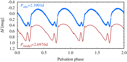
Figure 16: Comparison of the observed $I$-band light curve of OGLE-BLG-T2CEP-279 (blue dots) with the pulsation model (red curve). The period doubling effect is recognizable upon comparing consecutive maxima and minima. The model is vertically offset by 0.6.

Figure 17: Radius variation in two models differing only in their $T_{\rm eff}$ that show periodic modulation (upper panel) and deterministic chaos (lower panel).

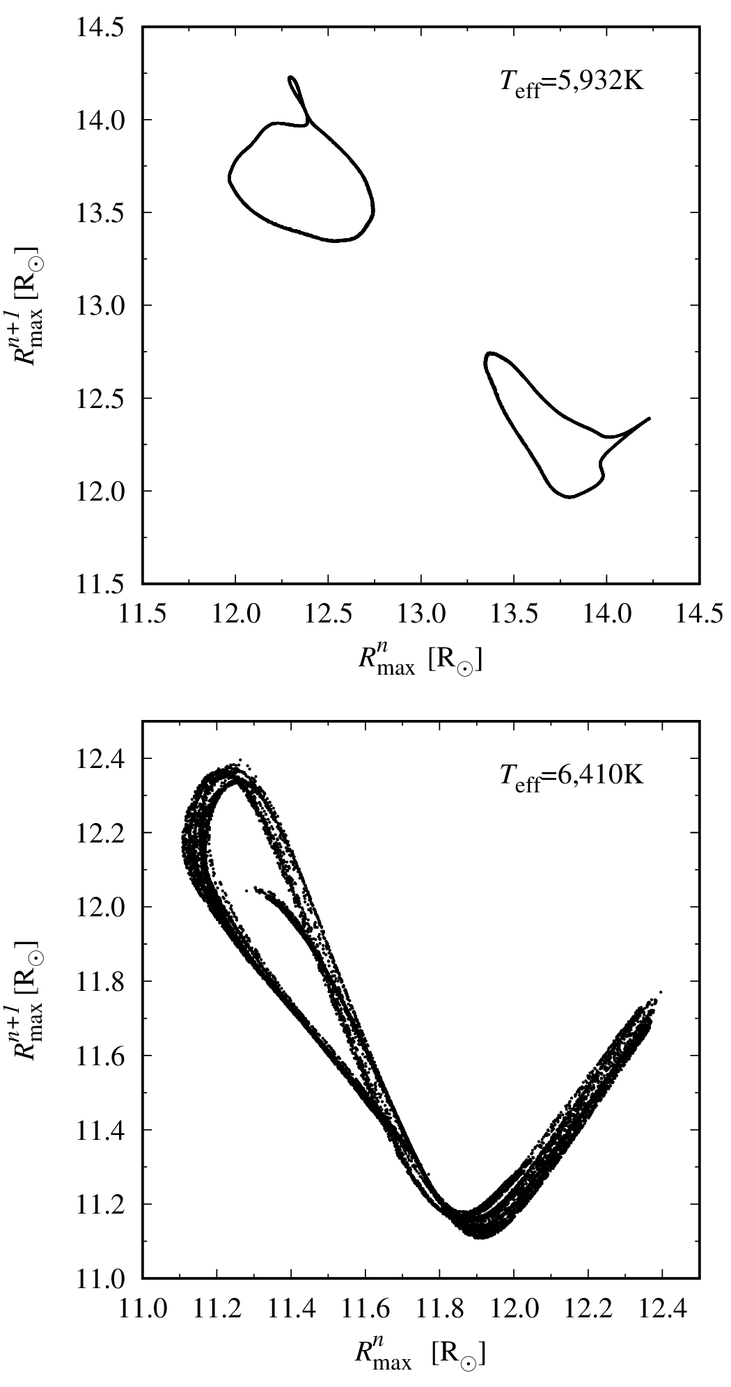
Figure 18: Maximum radius return maps for the models in Figure 17.

Figure 17 shows the radius variation for two models with $M$ = 0.55 $\mathrm{M}_{\odot}$, $L$ = 136 $\mathrm{L}_{\odot}$, $X$ = 0.76, $Z$ = 0.0001 and convective set A but with a reduced eddy-viscosity, $\alpha_{\rm m}$ = 0.05 (yielding unrealistic light curves). The two models differ only in $T_{\rm eff}$ = 5,932 $\mathrm{K}$ (upper panel) and $T_{\rm eff}$ = 6410 $\mathrm{K}$ (lower panel). Figure 18 shows the return map of maximum radii for these two models, plotting the maximum radii for each pulsation cycle $R_{\rm max}^{n}$ versus the preceding $R_{\rm max}^{n-1}$.

For the cooler $T_{\rm eff}$ = 5,932 $\mathrm{K}$ model, the upper panel of Figure 17 shows a cyclic modulation in the envelope of the period-doubled pulsation. The modulation period of $\simeq$ 57 d is longer than the pulsation period of $\simeq$ 2.3 d. The return map in the upper panel of Figure 18 is constructed from $\simeq$ 8,000 pulsation cycles and shows two loops, corresponding to alternating smaller and larger maximum radii. Since the modulation period is not commensurate with the pulsation period, the return maps develop a locus of points that form the closed lobes. Light curve modulation is common in RR Lyrae stars (Blazhko effect) and periodic pulsation modulation was recently discovered in BL Her variables (Smolec et al., 2018).

For the hotter $T_{\rm eff}$ = 6,410 $\mathrm{K}$ model, the radius variation appears irregular in the lower panel of Figure 17. The return map in the lower panel of Figure 18 reveals a strange attractor, an example of deterministic chaos in nonlinear models. Tracing time series from models is simple, but tracing chaotic dynamics in observations is difficult (e.g., Plachy et al., 2018). Chaotic dynamics is reported in a few type-II Cepheids with longer periods, in the RV Tau variable star range, and in semi-regular variable stars (e.g., Buchler et al., 1996; Kollath et al., 1998; Buchler et al., 2004; Plachy et al., 2018). While the $T_{\rm eff}$ = 6,410 $\mathrm{K}$  model has a shorter period, in the BL Her range, such models may provide insight into chaotic dynamics in pulsating stars (see Plachy et al., 2013; Smolec & Moskalik, 2014).

2.4.4 Binary Evolution Pulsators

Very-low-mass stars do not enter the classical instability strip within a Hubble time. However, mass loss from the more massive component in a close interacting binary can lead to a low-mass star that then evolves through the instability strip. The Binary Evolution Pulsator (BEP, OGLE-BLG-RRLYR-02792) is the prototype of this new class of pulsators (Pietrzynski et al., 2012; Smolec et al., 2013). The BEP’s variability is similar to an F-mode RR Lyrae pulsator but with a dynamical mass of $\simeq$ 0.26 $\mathrm{M}_{\odot}$.

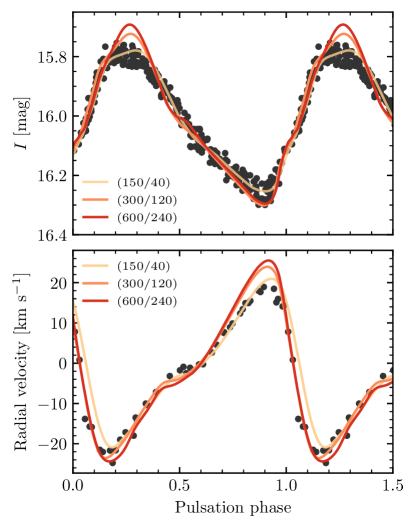
Figure 19: $I$-band light (upper panel) and radial velocity (lower panel) curves of the BEP OGLE-BLG-RRLYR-02792 as a function of pulsation phase. Observations are shown as circles (Pietrzynski et al., 2012) with the radial velocity multiplied by a projection factor of $p$ = 1.2. Model curves are shown at three resolutions labeled by ($N/N_{\rm outer}$).

Following Smolec et al. (2013), we adopt $M$ = 0.26 $\mathrm{M}_{\odot}$, $L$ = 33 $\mathrm{L}_{\odot}$, $T_{\rm eff}$ = 6,910 $\mathrm{K}$, $X$ = 0.7, $Z$=0.01, and convective set A. Figure 19 shows $I$-band light curves and radial velocity curves for the BEP models. Results for a coarse grid ($N/N_{\rm outer}$=150/40, gold curves) qualitatively match these observations and have a period of 0.6373 d close to the observed 0.6275 d period. We also show results for a medium grid (300/120, orange curves) and a fine grid (300/120, red curves). The differences are most pronounced around maximum and minimum light. The shape of the light and radial velocity curves approach convergence only on grids with $\gtrsim$  600 cells. The amplitude of the model curves are sensitive to convective parameters and can be fine-tuned for a better match with observations.

2.4.5 Blue Large Amplitude Pulsators

The origin of BLAPs, introduced in Section 1, is unknown. They have been modeled as $\simeq$ 0.3 $\mathrm{M}_{\odot}$ shell H-burning stars that are progenitors of low mass WDs and $\simeq$ 1.0 $\mathrm{M}_{\odot}$ stars undergoing core He-burning (Pietrukowicz et al., 2017; Romero et al., 2018; Wu & Li, 2018; Byrne & Jeffery, 2018). Though mass loss in a close interacting binary must be invoked for both hypotheses, none of the BLAPs are known to be in a binary. Figure 1 shows that BLAPs are located near sdBVs in the HR diagram. The latter have non-canonical abundance profiles that are strongly affected by radiative levitation (see Section 6.2). Following the linear study of Romero et al. (2018), we adopt $Z$ = 0.05, to account for the increased envelope metallicity caused by radiative levitation.

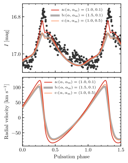
Figure 20: $I$-band light (upper panel) and radial velocity (lower panel) curves for OGLE-BLAP-011. Observations are shown as circles (Pietrukowicz et al., 2017). RSP models for three convective sets are shown under the $\simeq$ 1.0 $\mathrm{M}_{\odot}$ core He-burning hypothesis. Pulsation periods of the models range between 34.27 and 34.34 min and the observed period is 34.87 min.

We explored nonlinear models with $M$ = 1.0 $\mathrm{M}_{\odot}$, $T_{\rm eff}$ =30,000 $\mathrm{K}$, $L$ = 430 $\mathrm{L}_{\odot}$, and three convection parameter sets. These envelope models used $N$ = 280, $N_{\mathrm{outer}}$ = 140, $T_{\mathrm{anchor}}$ = 2$\times$10⁵ K, and $T_{\mathrm{inner}}$ = 6$\times$10⁶ K. The LNA analyses show the F and 1O modes are unstable. Figure 20 compares the OGLE-BLAP-011 and 1O-mode ($P\simeq 35$ min) model $I$-band light curves. The qualitative agreement is reasonable. Figure 20 shows the model radial velocity curves have amplitudes of $\simeq$ 200 km s^-1, a pronounced temporal asymmetry, and light maxima that are narrower than light minima.

These BLAP models lie far off the classical instability strip so that the initial model builder (see Section 2.2.1), which is optimized for classical pulsators, failed to relax the initial models to complete hydrostatic equilibrium. An option is to switch off the relaxation process and commence the time integration with a near-hydrostatic-equilibrium initial model. The price to pay is the LNA growth rates are only indicative, not accurate.

Figure 21 shows the evolution of $\Gamma$ for the $(\alpha$,$\alpha_{\rm m})$=(1.5,0.1) model in Figure 20. Before $\simeq$ 10 d, $\Gamma$ fluctuates around a mean $\simeq$ 7.5$\times$10^-3. The fluctuations diminish with time but $\Gamma$ remains above the LNA value of 6.25$\times$10^-3 up to $\simeq$ 30 d. Between 30-50 d $\Gamma$ diminishes and approaches zero, the sign that the nonlinear pulsation saturates at its terminal amplitude, yielding the results of Figure 20. In contrast to $\Gamma$, the period of the nonlinear pulsations remain close to the LNA period. In cases where the initial model cannot be relaxed, the initial $\Gamma$ should not be expected to match the LNA analysis.

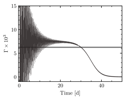
Figure 21: Evolution of the RSP growth rate $\Gamma$ starting from the unrelaxed initial model for convection set b in Figure 20. The horizontal line shows the LNA growth rate computed from the unrelaxed initial model.

2.4.6 High Amplitude Delta Scuti

High-amplitude $\delta$ Scuti (HADS) pulsators are defined to have $V$-band light curve amplitudes greater than 0.1 mag. HADS lie close to the main-sequence (MS; see Figure 1), where growth rates are usually much smaller than those for RR Lyrae stars or classical Cepheids. This implies long time integrations are needed to drive nonlinear pulsations to saturation.

We consider a stellar model with $M$ = 2 $\mathrm{M}_{\odot}$, $L$ = 30 $\mathrm{L}_{\odot}$, $T_{\rm eff}$ = 6,900 $\mathrm{K}$, $X$ = 0.7, $Z$=0.01, and convective set A. This represents a star evolving towards the Hertzsprung gap. The LNA analysis of the initial model reveals that the F and 1O modes are linearly unstable, with growth rates of 1$\times$10^-6 and 6$\times$10^-5, respectively.

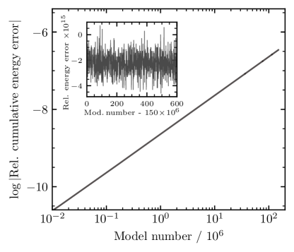
Figure 22: Evolution of the relative cumulative energy error from model 10,000 ($\simeq$ 15 cycles) to $\simeq$ 150 million (at $\simeq$ 250,000 cycles). The inset shows the per-step relative energy error over a cycle (600 steps).

Section 3 emphasizes the importance of numerical energy conservation. Figure 22 shows the evolution of the relative cumulative error in the energy for a 250,000 cycle integration ($\simeq$ 150 million time steps, at 600 steps per cycle). The relative cumulative error grows from $\simeq$ 3$\times$10^-11 after about 15 cycles to $\simeq$ 3$\times$10^-7 after 250,000 cycles. The inset figure shows that the per-step relative error in the energy scatters around $-$2.5$\times$10^-15 but is systematically different than zero.

Figure 23 shows that after 70,000 cycles the asymmetric $V$-band light curves have an amplitude of $\simeq$ 0.2 mag. The dominant pulsation period is 0.127 d, close to the LNA period of 0.1269 d for the 1O-mode. The amplitude, though, varies cyclically over about four pulsation cycles, reflecting the presence of the F-mode. Continuing the integration to 130,000 cycles leads to a more saturated light curve with an amplitude of $\simeq$ 0.3 mag and an unchanged dominant pulsation period. Extending the integration to 250,000 cycles does not lead to any significant changes.

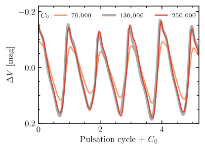
Figure 23: $V$-band light curves of the $\delta$ Sct model at three stages during a very-long ($\simeq$ 150 million time step) integration. For each stage, we plot the light curve for 5 pulsation cycles. The legend gives the cycle numbers when the snapshots were taken.

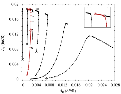
Figure 24: Evolution of fractional radius amplitude, $\delta R/R$, for the 1O mode, $A_{1}$ and F mode, $A_{0}$. Eight trajectories begin at locations marked with a cross. Circles mark 1,000 d intervals along trajectories. The red curve corresponds to the model in Figure 23 with the three open circles marking the amplitudes after 70,000, 130,000, and 250,000 cycles. The inset on the upper right zooms into the slowing amplitude evolution of the red curve late in the simulation.

The robustness in the light curves between 130,000 and 250,000 cycles might suggest that the long-term behavior is that of a double-mode HADS model. However, additional integrations with different initial perturbations, chosen to more adequately sample the neighboring amplitude phase space, are necessary to assess the possible mode selection. Figure 24 shows the evolution of these integrations in the amplitude-amplitude diagram using the analytical signal method (e.g., Kolláth et al., 2002). The amplitude behavior of the model integration shown in Figure 23 is traced out by the red line. After initially rapid evolution, all the amplitude trajectories develop an arc along which evolution slows markedly. The model in Figure 23 and neighboring trajectories bend to the left toward smaller F-mode amplitudes. Their likely final state is that of a single-periodic 1O pulsation. In contrast, the two right-most trajectories bend to the right towards larger, more dominant, F-mode amplitudes. Despite the limited sampling of phase space in Figure 24, we cautiously conclude that the most likely long-term outcome of this $\delta$ Sct model is a single-periodic 1O-mode or F-mode pulsator depending on the initial conditions (see Section 2.2.4).

3 Energy Conservation

For the following discussion we define the total energy $E$ of a model to be the sum of the internal, potential, and kinetic energies, ignoring rotational and turbulent energy which are currently not included in the energy accounting. To support improved numerical energy conservation, MESAstar provides an option to use what we call the dedt-form of the energy equation:

$$\frac{\mathrm{D}e}{\mathrm{D}t}=\epsilon-\frac{\partial}{\partial m}\left(L+p\mathcal{A}\,u\right)-\frac{\mathrm{D}}{\mathrm{D}t}\left(\frac{1}{2}u^{2}-\frac{Gm}{r}\right)~{}.$$ (8)

This form was introduced in Paper IV and provides an alternative to the dLdm-form of the energy equation (Equation (11) in Paper I). When the time derivative terms are combined, the result is more easily recognizable as an equation for the time evolution of local specific total energy (left hand side) due to local source terms ($\epsilon$) and local fluxes between cells (the $\partial/\partial m$ term):

$$\frac{\mathrm{D}}{\mathrm{D}t}\left(e+\frac{1}{2}u^{2}-\frac{Gm}{r}\right)=\epsilon-\frac{\partial}{\partial m}\left(L+p\mathcal{A}\,u\right)~{}.$$ (9)

The error in numerical energy conservation $E_{\rm error}$ is the extent to which the time- and mass-integrated Equation (9) is not satisfied when solved in a discretized, finite-mass form. This section discusses recent efforts to improve numerical energy conservation in MESAstar.

Recall (from Paper I, Section 6.3) the generalized Newton-Raphson scheme used by MESAstar to solve the stellar equations

$$0=\vec{F}(\vec{y})=\vec{F}(\vec{y}_{i}+\delta\vec{y}_{i})=\vec{F}(\vec{y}_{i})+\left[\frac{d\vec{F}}{d\vec{y}}\right]_{i}\delta\vec{y}_{i}+O(\delta\vec{y}_{i}^{\,2})\,,$$ (10)

where $\vec{y}_{i}$ is the trial solution for the $i$-th iteration, $\vec{F}(\vec{y}_{i})$ is the residual, $\delta\vec{y}_{i}$ is the correction, and $[d\vec{F}/d\vec{y}]_{i}$ is the Jacobian matrix. The residual is the left over difference between the left- and the right-hand sides of the equation we are trying to solve, while the correction is the change in the primary variable that is calculated by Newton’s rule. The solver generates a series of trial solutions until it produces one that is acceptable according to given convergence criteria. In MESAstar the trial solution is not accepted until the magnitudes of all corrections and residuals become smaller than specified tolerances. If no acceptable trial solution has been found in the allowed maximum number of iterations, the solver rejects the attempt and forces a retry with a smaller time step.

If the numerical accuracy of the partial derivatives forming the Jacobian matrix is not excellent, the reduction in magnitude of the residuals can stall after a few iterations. For this reason, MESAstar has provided a means to use a tight tolerance on residuals for an initial sequence of iterations and then switch to a much relaxed tolerance if no acceptable solution has been found. The benefit of this is that residuals will be driven down when possible, but if the residuals stall at a level above the initial tolerance, the system will still be able to take a step as long as the corrections can be adequately reduced. The cost of relaxing the tolerance for residuals of the total energy equation is the creation of numerical energy conservation errors. To obtain good numerical energy conservation we must be able to drive down residuals to low levels, and to do that we must have numerically accurate partial derivatives. This has motivated a major effort to improve partials, and we can now require the solver to keep iterating until it reduces the residuals to a low level that gives good numerical energy conservation. The most significant changes to improve the numerical accuracy of partials were in the eos module and are discussed in Appendix A.1.

3.1 Gold Tolerances

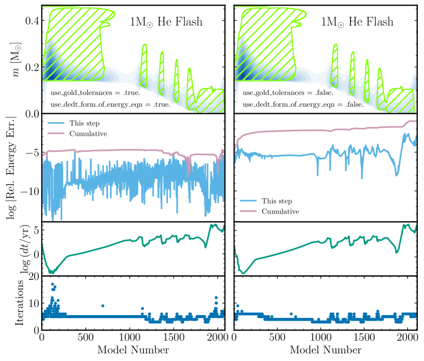
Figure 25: Evolution of a 1 $\mathrm{M}_{\odot}$ model during the He flash and core He burning using gold tolerances and the dedt-form of the energy equation (left panel), and without gold tolerances and using the dLdm-form of the energy equation (right panel). The first panel shows a Kippenhahn plot, where green hatched regions are convective and blue shading shows region of nuclear energy generation. The second panel shows the absolute error in energy conservation divided by the total stellar energy, both per step and cumulative. The third panel shows the time step, while in the fourth panel we report the number of iterations required by the Newton-Raphson solver. Gold tolerances keep the cumulative errors small during the He flash at the price of a larger number of iterations during the first $\approx$200 time steps.

To improve energy conservation, a new standard “gold tolerances” is now the default in MESAstar. This uses tight tolerances that apply even after an arbitrarily large number of iterations. As a result, steps with poor residuals will be rejected, thereby ensuring that if a run succeeds with gold tolerances enabled while using the total energy equation given above, it will have good energy conservation. To show example improvements from this new strategy, in Table 5 we report the results of calculations of a $1\,\mathrm{M}_{\odot}$ model during the main sequence and the He flash with gold tolerances and compare to the old approach. The $1\,\mathrm{M}_{\odot}$ models are evolved from the ZAMS until the core H mass fraction reaches a value of $10^{-6}$. The He flash models start at off-center He ignition and terminate when the core He mass fraction drops to $10^{-3}$. The cumulative energy error is the sum of the energy conservation errors at each of the steps. The relative cumulative energy error is the cumulative energy error divided by the final total energy. This is now much less than 1% during the He flash, a notoriously difficult evolutionary phase from the numerical perspective. The evolution of the errors in energy conservation, as well as the number of iterations required by the solver and the adopted time step, are shown in Figure 25 for the He flash runs. This figure clearly show the superiority of the model adopting gold tolerances and the dedt-form of the equation in terms of energy conservation.

Not all cases in the MESAstar test suite are currently able to use gold tolerances. This is primarily because of remaining problems with the numerical accuracy of certain partials, especially in the PC EOS (Potekhin & Chabrier, 2010) that is used by WD models (see Appendix A.1) and on the boundary between the OPAL EOS (Rogers & Nayfonov, 2002) and the SCVH EOS (Saumon et al., 1995). There are also problems with the numerical accuracy of some partials associated with nuclear reactions at the high temperatures encountered during late stages of evolution, such as Si burning. To address these situations, there are controls to allow gold tolerances to be turned off automatically for steps that either require use of the PC EOS or that have extremely high temperatures. To provide feedback, the value of the relative cumulative energy error is monitored and a warning message is written if it exceeds a specified value (2% is the default setting).

Table 5: Relative cumulative energy error for $1\,\mathrm{M}_{\odot}$ runs.

	Main Sequence	He Flash
dedt + Gold Tolerances	0.3%	0.0006%
dLdm	14%	12%

3.2 Definition of $\epsilon_{\mathrm{nuc}}$ Source Term

Previous MESA papers have not given a precise definition of $\epsilon_{\mathrm{nuc}}$. Motivated by numerical convenience, MESA formerly exploited the fact that the $\epsilon$ source term contained the sum of $\epsilon_{\mathrm{grav}}$ and $\epsilon_{\mathrm{nuc}}$ and included the response of the internal energy to composition changes due to nuclear reactions in $\epsilon_{\mathrm{nuc}}$ instead of in $\epsilon_{\mathrm{grav}}$. However, since the dedt-form does not include $\epsilon_{\mathrm{grav}}$, this is no longer an appropriate choice.

In the current approach, $\epsilon_{\mathrm{nuc}}$ is evaluated in the net module as a sum over reactions. Schematically,

$$\epsilon_{\mathrm{nuc}}=N_{\mathrm{\!A}}\sum_{\mathrm{reactions}}\left(Q_{i}-Q_{\nu,i}\right)R_{i}~{},$$ (11)

where $R_{i}$ is the molar rate of reaction $i$, $Q_{i}$ is the change in rest mass energy between the products and reactants, and $Q_{\nu,i}$ is the per-reaction average energy of the neutrino (if present). We note the equivalence

$$\sum_{\mathrm{reactions}}Q_{i}R_{i}\equiv-\sum_{\mathrm{isotopes}}M_{i}c^{2}\dot{Y_{i}}~{},$$ (12)

where $M_{i}$ is the rest mass of isotope $i$ and $\dot{Y}_{i}$ is the rate of change of the molar fraction. The approx family of MESA nuclear networks exploit this equivalence and do not strictly follow Equation (11). The right hand side of Equation (12) is a common nuclear physics definition of $\epsilon_{\mathrm{nuc}}$ (e.g., Equation 11 in Hix & Meyer, 2006). The MESA definition of $\epsilon_{\mathrm{nuc}}$ differs in subtracting off the nuclear neutrino losses, thus enforcing the assumption that they free-stream out of the star.

3.3 Mass Changes

The methods described above perform well for numerical energy conservation when the stellar mass is constant, but extensions are necessary for cases where the mass changes. For energy accounting, we must specify the amount of energy we expect the new mass to introduce and the amount we expect departing mass to remove. To that end we assume that mass being added has the same specific energy as the surface of the model at the start of the step. For mass being removed, we assume that it leaves with a specific energy between what it had at the start of the step and the value at the surface at the start of the step. The exact amount depends on the amount of energy that leaks out of the material as it approaches the surface during the time step. For low rates of mass loss there will be adequate time for the material to adjust so that it leaves with the initial surface value, but for high rates there may not be enough time for adjustment, so that it leaves with a specific energy closer to its starting value. The details of this are presented below.

In addition to providing accurate accounting for the total energy of the model, it is important to ensure that the energy changes from mass loss or gain are distributed properly within the model. As a guide for this we use the analytic calculations of Townsley & Bildsten (2004). Our new procedure improves upon these by also calculating the distribution of energy in systems with long thermal times, allowing MESA to handle the limit of rapid accretion. We confirm the numerical energy conservation of this method using the $>20$ cases in the MESAstar test suite that have mass changes and fully support gold tolerances and the dedt-form of the energy equation. Using the new scheme, each of these completes the test run with a cumulative error in total energy $<2$ %. In addition, test cases that depend on the internal distribution of accretion heating continue to yield the expected results.

3.3.1 Methodology

Because MESA works on a Lagrangian mesh, it handles accretion and mass loss in a two-stage process (Paper III, Section 7). In stage I the masses of certain cells are increased or decreased as needed to give the desired end-of-step total mass, but no attempt is made to ensure energy conservation at this stage. In stage II the model thus produced is evolved in time by an amount $\delta t$. This separation of stages means that the time step is only taken for a model of fixed mass. However, because the energy of the model changes in stage I, a correction must be added to stage II to make the overall step consistent with energy conservation. Thus, we introduce a new source term $\epsilon_{\dot{M}}$ that accounts for the heating associated with mass changes.

The change in the mass of cell $k$ during stage I results from the difference between the outward mass flux $F_{m}$ through each cell face. This flux obeys

$$dm_{{\rm mid},k}-dm_{{\rm start},k}=\delta t\left(F_{m,k+1}-F_{m,k}\right)$$ (13)

and

$$M_{{\rm mid}}-M_{{\rm start}}=-\delta tF_{m,1}=\delta t\dot{M}.$$ (14)

During stage I the temperature, density, and velocity of each cell are held fixed but the composition is updated to track the flow of material between cells. The subscript start is used for quantities at the start of stage I. The subscript mid is used for quantities at end of stage I, which is the start of stage II. No subscript is used for quantities evaluated at the end of the time step (after stage II). There is no mass change during stage II, so $dm_{k}=dm_{{\rm mid},k}$. In the following we write $dm_{k}$ rather than $dm_{{\rm mid},k}$.

The change in energy for cell $k$ during stage I is

$$E_{{\rm mid},k}-E_{{\rm start},k}= dm_{k}\mathcal{E}_{{\rm mid},k}-dm_{{\rm start},k}\mathcal{E}_{{\rm start},k}$$ (15)

$$= dm_{k}\left(\mathcal{E}_{{\rm mid},k}-\mathcal{E}_{{\rm start},k}\right)$$

$$+(dm_{k}-dm_{{\rm start},k})\mathcal{E}_{{\rm start},k},$$

where $\mathcal{E}_{k}$ is the total specific energy of cell $k$, given by the sum of specific potential, kinetic, and internal energies. Neglecting changes in specific energy owing to changes in composition, the difference in $\mathcal{E}_{k}$ across stage I is

$$\mathcal{E}_{{\rm mid},k}-\mathcal{E}_{{\rm start},k}=\left(\frac{Gm_{k,\rm C}}{r_{k,\rm C}}\right)_{{\rm start}}-\left(\frac{Gm_{k,\rm C}}{r_{k,\rm C}}\right)_{{\rm mid}}~{}.$$ (16)

where $m_{k,\rm C}$ and $r_{k,\rm C}$ are the mass coordinate and radius at the center of mass of the cell (Paper IV).

We now introduce $\epsilon_{k,{\rm I}}$, the effective source term in cell $k$ during stage I. This is defined by writing the change in energy in flux-conservative form as

$$E_{{\rm mid},k}-E_{{\rm start},k} =\delta t\left(dm_{k}\epsilon_{k,{\rm I}}+F_{e,k+1,{\rm I}}-F_{e,k,{\rm I}}\right),$$ (17)

where $F_{e,k,{\rm I}}$ is the outward flux of energy across face $k$ owing to work and material passing through face $k$. Inserting Equation (15) and rearranging we obtain

$$\epsilon_{k,{\rm I}}\equiv \frac{\mathcal{E}_{{\rm mid},k}-\mathcal{E}_{{\rm start},k}}{\delta t}+\frac{\mathcal{E}_{{\rm start},k}}{\delta t}\left(1-\frac{dm_{{\rm start},k}}{dm_{k}}\right)$$

$$-\frac{F_{e,k+1,{\rm I}}-F_{e,k,{\rm I}}}{dm_{k}}.$$ (18)

The energy flux is

$$F_{e,k,{\rm I}} =p_{{\rm face},k}\mathcal{A}_{k}\hat{v}_{k,{\rm I}}+\mathcal{E}_{{\rm face},k}F_{m,k}\,,$$ (19)

where

$$\hat{v}_{k,{\rm I}}\equiv\frac{r_{{\rm mid},k}-r_{{\rm start},k}}{\delta t}~{},$$ (20)

and the face values $\mathcal{E}_{\rm face}$ are interpolated from the cell values $\mathcal{E}_{{\rm start}}$. The radial coordinate after state I is calculated using the updated cell masses, holding cell densities fixed. The change in total energy of the model during stage I is

$$\sum_{k}\left(E_{{\rm mid},k}-E_{{\rm start},k}\right)= -\delta t\left(p_{{\rm face},1}\mathcal{A}_{1}\hat{v}_{1,{\rm I}}+\mathcal{E}_{{\rm face},1}F_{m,1}\right)$$

$$+\delta t\sum_{k}dm_{k}\epsilon_{k,{\rm I}}~{}.$$ (21)

The term in parentheses on the right-hand side accounts for the energy of new material entering or leaving the model and the work done in the process. The additional $\epsilon_{k,{\rm I}}$ term implies the need for a corrective source term $\epsilon_{\dot{M}}$ which must be added during stage II so that energy is properly accounted for.

To determine this new source we consider the ratio of the thermal time scale

$$\tau_{{\rm th},k}\equiv\left|\frac{x_{m}c_{{\rm p}}T(\nabla_{\rm rad}-\nabla_{\rm ad})}{L}\right|_{{\rm start},k},$$ (22)

to the mass-change time scale

$$\tau_{{\rm m},k}\equiv\left|\frac{x_{m}}{F_{m}}\right|_{{\rm start},k},$$ (23)

where $x_{m,k}$ is the mass above face $k$. When this ratio is small the thermodynamic state of material is a function primarily of depth (Sugimoto, 1970; Sugimoto & Nomoto, 1975). This means that as material moves from cell to cell it is a good approximation to the time evolution to suppose that it adopts the state of whichever cell it is in (Paper III). In the opposing limit ($\tau_{\rm th}\gg\tau_{\rm m}$) the entropy of material adjusts minimally as it moves from cell to cell.

We account for the effects of the thermal and mass-change time scales by tracking the heating of material as it moves from cell to cell in stage I and estimating what fraction of that heat is released as part of $L$ versus carried by the material. Consider the path taken by an infinitesimal fluid element as it moves from face $k$ to face $k+1$ due to accretion. Over the course of this adjustment the material changes state and releases some heat. We take this heat to be given by

$$dq_{k}=-\delta t\epsilon_{k,{\rm I}}\frac{dm_{k}}{dm_{\rm pass,k}},$$ (24)

where

$$dm_{\rm pass,k}=dm_{{\rm start},k}+\delta t\left(\max(0,F_{m,k+1})-\min(0,F_{m,k})\right)$$ (25)

is the total mass of material that at any point during stage I was inside cell $k$. This evenly distributes the heating which occurs in a cell over all material that starts in, ends in, or passes through the cell. When the thermal time is long, however, the fluid does not have a chance to release all of this heat before it has finished crossing the cell. We estimate the fraction of this heat it releases as the leak fraction

$$f_{{\rm leak},k} \equiv\min\left(1,\frac{\tau_{{\rm m},k}}{\tau_{{\rm th},k}}\right).$$ (26)

This parameterises the extent to which material flowing through a cell follows the implied energy gradient ($f_{{\rm leak},k}\approx 1$) versus evolving adiabatically ($f_{{\rm leak},k}\ll 1$).

We define $\delta E_{k,j}$ to be the amount of energy that the material which ends up in cell $j$ had not leaked by the time it reached face $k$. This is zero for $k=1$ and for $k>j$, and for all other faces is given by

$$\delta E_{k+1,j}=(1-f_{{\rm leak},k})\left(\delta E_{k,j}+dq_{k}\mathcal{M}_{k,j}\right),$$ (27)

where $\mathcal{M}_{k,j}$ is the amount of material which ends in cell $j$ which passes through cell $k$ during stage I. The heat which is actually released in cell $k$ is then given by

$$\epsilon_{\dot{M},k}=\frac{\delta E_{k,k}+\sum_{j\neq k}f_{{\rm leak},k}\left(\delta E_{k,j}+dq_{k}\mathcal{M}_{k,j}\right)}{\delta tdm_{k}}.$$ (28)

This is our new corrective source term. The same procedure may be used in the case of mass loss, but with $\delta E_{N+1,j}=0$ instead of $\delta E_{1,j}$ and $-1$ in the subscript on the left-hand side of Equation (27) rather than $+1$. In the limit of long thermal times most heat is retained and the resulting evolution is adiabatic. In the limit of short thermal times we recover the results of Paper III.

Along the lines of Equation (17), the energy change of cell $k$ during stage II may now be written in flux-conservative form as

$$E_{k}-E_{{\rm mid},k} =\delta t\left[dm_{k}(\epsilon_{\dot{M},k}+\epsilon)+F_{e,k+1,\mathrm{II}}-F_{e,k,\mathrm{II}}\right],$$ (29)

where

$$F_{e,k,{\rm II}}=L_{k}+p_{{\rm face},k}\mathcal{A}_{k}\hat{v}_{k,{\rm II}}$$ (30)

and

$$\hat{v}_{k,{\rm II}}\equiv\frac{r_{k}-r_{{\rm mid},k}}{\delta t}~{}.$$ (31)

MESA solves Equation (29) when using the dedt-form with mass changes. Because the time evolution is implicit all sources are evaluated at the end of stage II. Nuclear burning is evaluated as if material spends the whole step in the cell in which it ends stage I. While this is usually a good approximation it may break down when $\delta t\dot{M}$ is large relative to the masses of cells in burning regions.

When $\dot{M}\geq 0$ the above procedure for redistributing energy is conservative, so that

$$\sum_{k}\epsilon_{k,\mathrm{I}}\delta tdm_{k}+\sum_{k}\epsilon_{\dot{M},k}\delta tdm_{k}=0.$$ (32)

The first sum represents the effect of stage I; the second sum represents the effect of stage II. When $\dot{M}<0$ the equality is instead

$$\sum_{k}\epsilon_{k,\mathrm{I}}\delta tdm_{k}+\sum_{k}\epsilon_{\dot{M},k}\delta tdm_{k} =-\delta E_{1,0},$$ (33)

with the additional term $\delta E_{1,0}$ being the energy carried out of the star. This term is explicitly accounted for in the MESA energy budget, so in both cases energy is properly accounted for.

3.3.2 Results

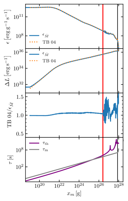
Figure 26: Comparison of $\epsilon_{\dot{M}}$ and the analytic accreting heating expression from Townsley & Bildsten (2004) (TB 04) for a $0.33\,\mathrm{M}_{\odot}$ He WD accreting He and N at a rate of $10^{-5}\mathrm{M}_{\odot}\,{\mathrm{yr}}^{-1}$. The first panel shows both as functions of depth $x_{m}$. The second panel shows the same but integrated inward with respect to mass. The third panel shows the ratio of the TB 04 expression to $\epsilon_{\dot{M}}$. The final panel shows the thermal time scale $\tau_{\rm th}$ and the mass-change time scale $\tau_{\rm m}$. All material to the left of the red vertical line is material which is new in this time step. To the right of the vertical black line MESA transitions to a Lagrangian mesh which continues over the remainder of the core.

To examine the behavior of $\epsilon_{\dot{M}}$ we modeled a $0.33\,\mathrm{M}_{\odot}$ WD accreting He and N at a rate of $10^{-5}\,\mathrm{M}_{\odot}\,{\mathrm{yr}}^{-1}$. The first panel of Figure 26 shows a profile of $\epsilon_{\dot{M}}$ along with the analytic accretion heating calculations of Townsley & Bildsten (2004). For the most part the two agree closely. The second panel shows the mass integral of the same inward from the surface while the third shows their ratio. Around $x_{m}\approx 10^{26}{\rm g}$, $\tau_{\rm th}$ becomes long relative to $\tau_{\rm m}$ and the two prescriptions differ because that of Townsley & Bildsten (2004) is only applicable where $\tau_{\rm th}\ll\tau_{\rm m}$. The $\epsilon_{\dot{M}}$ term handles both limits.

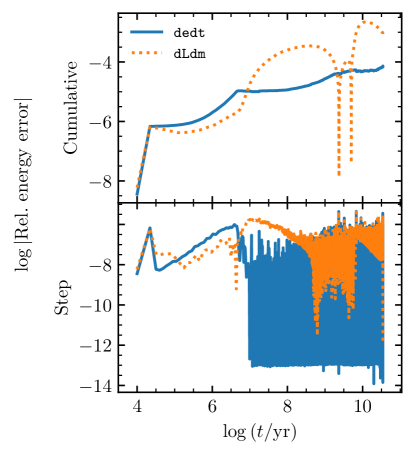
Figure 27: Comparison of energy conservation for a $0.3\,\mathrm{M}_{\odot}$ He WD model accreting an H/He mixture at a rate of $10^{-10}\,\mathrm{M}_{\odot}\,{\mathrm{yr}}^{-1}$. The upper panel shows the relative cumulative error and the lower shows the error in each step.

To demonstrate improved energy conservation during mass changes with the dedt-form we model accretion onto a $0.3\,\mathrm{M}_{\odot}$ He WD with an initial $\log(T_{\mathrm{c}}/\mathrm{K})=6.7$. The accretion rate is fixed at $10^{-10}\,\mathrm{M}_{\odot}\,{\mathrm{yr}}^{-1}$. Nuclear reactions are disabled throughout the run. This is repeated with the dLdm-form. The relative cumulative error in energy conservation is shown in the upper panel of Figure 27, and the relative error in each step is shown in the lower panel. Near the beginning of the run there is a period where the dLdm-form performs better, however at those early times both forms do a good job, conserving energy to one part in $\sim 10^{5}$. At later times the dedt-form produces less error, staying below one part in $10^{4}$ while the dLdm-form yields cumulative errors greater than one part in $10^{3}$.

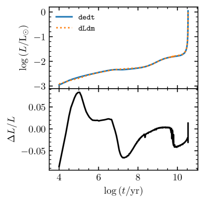
Figure 28: Comparison of the surface luminosity for a $0.3\,\mathrm{M}_{\odot}$ He WD model accreting a H/He mixture at $10^{-10}\,\mathrm{M}_{\odot}\,{\mathrm{yr}}^{-1}$ (same as Figure 27). The upper panel shows the surface luminosity and the lower shows the relative difference between the dLdm-form and the dedt-form, all as functions of time since the start of accretion.

We prefer using the dedt-form  because of its improved energy conservation and handling of long thermal times. We now explore the consequences for stellar evolution of these different prescriptions. The upper panel of Figure 28 shows the luminosity for the same case as Figure 27, again for both the dedt-form and the dLdm-form. The difference is shown in the lower panel. The largest differences are at early times as the models adjust to the accretion. After that, both yield results similar to a few percent, and the relative difference only improves as the luminosity increases. Figure 29 shows $T_{\mathrm{c}}$ for the same two runs as a function of time. The differences are small. This is because the core lies beneath the region where cell masses are adjusted significantly, so the precise handling of mass changes only matters for the core insofar as the core temperature is sensitive to the luminosity.

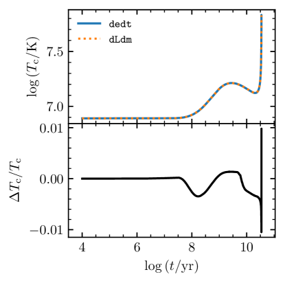
Figure 29: Comparison of the central temperature for a $0.3\,\mathrm{M}_{\odot}$ He WD model accreting a H/He mixture at $10^{-10}\,\mathrm{M}_{\odot}\,{\mathrm{yr}}^{-1}$ (same as Figure 27). The upper panel shows the central temperature and the lower shows the relative difference between the dLdm-form and the dedt-form, all as functions of time since the start of accretion.

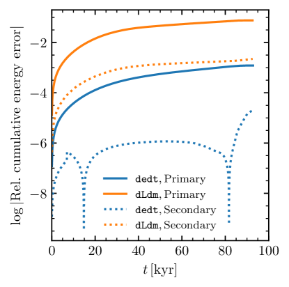
Figure 30: Comparison of energy conservation for the case of Figure 4 of Paper III: a binary system with mass transfer from the $8\,\mathrm{M}_{\odot}$ primary to the $6.5\,\mathrm{M}_{\odot}$ secondary and an initial orbital period of $3$ days. The relative cumulative energy error computed using both the dedt- and dLdm-forms is shown as a function of time after the start of accretion.

Mass changes are ubiquitous in binary stellar evolution. To demonstrate the effect of the dedt-form we model the evolution of a binary system with an $8\,\mathrm{M}_{\odot}$ primary and a $6.5\,\mathrm{M}_{\odot}$ secondary with an initial orbital period of $3$ days. This is the same example as in Figure 4 of Paper III. The relative cumulative error in energy conservation is shown in the upper panel of Figure 30. The model is also run with the dLdm-form. The errors are shown independently for the primary and the secondary. Figure 31 compares the mass transfer rate for this system computed using each energy equation. The differences are typically of order $1$ %.

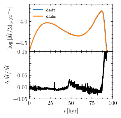
Figure 31: Comparison of mass transfer rates for the case of Figure 4 of Paper III: a binary system with mass transfer from the $8\,\mathrm{M}_{\odot}$ primary to the $6.5\,\mathrm{M}_{\odot}$ secondary and an initial orbital period of $3$ days. The upper panel shows the mass transfer rate computed using both the dedt- and dLdm-forms as a function of time after the start of accretion. Both are similar to the corresponding curves in Figure 4 of Paper III. The lower panel shows the relative difference between $\dot{M}$ computed with the dedt- and dLdm-forms. The spike at the end is due to mass transfer terminating at slightly different times.

4 Rotation

For a rigidly-rotating star in hydrostatic equilibrium, surfaces of constant pressure (isobars) coincide with the equipotential surfaces defined by the Roche potential $\Psi$,

$$\Psi(r,\theta)=\Phi(r,\theta)-\frac{r^{2}\Omega^{2}\sin^{2}\theta}{2},$$ (34)

where $\Phi$ is the standard Newtonian potential, $\theta$ is the polar angle, and $\Omega$ is the angular frequency of rotation. In one-dimensional stellar evolution calculations the effects of rotation on the stellar structure are usually captured by a simple modification of the stellar equations. These retain their regular form, but include two correction factors,

$$f_{P}=\frac{4\pi r_{\Psi}^{4}}{Gm_{\Psi}S_{\Psi}}\frac{1}{\langle g^{-1}\rangle},\quad f_{T}=\left(\frac{4\pi r_{\Psi}^{2}}{S_{\Psi}}\right)^{2}\frac{1}{\langle g\rangle\langle g^{-1}\rangle},$$ (35)

where $r_{\Psi}$ is the volume-equivalent radius of an isobar, and $m_{\Psi}$ and $S_{\Psi}$ are the mass inside that isobar and its surface area respectively (Kippenhahn & Thomas, 1970; Endal & Sofia, 1976). The effective gravity is $g=|\nabla\Psi|$, while $\langle g\rangle$ and $\langle g^{-1}\rangle$ are surface averages over the equipotential.

This approach is still applicable to the case of a differentially-rotating star under the assumption of shellular rotation, in which shells are rigidly-rotating, isobaric surfaces with rotation frequency $\Omega_{\Psi}$ (Endal & Sofia, 1976; Zahn, 1992). The averages in Equation (35) are performed over each isobar (Meynet & Maeder, 1997).

Until now, MESA used the method of Endal & Sofia (1976), which considers deviations of the Roche potential from spherical symmetry (Kopal, 1959), to compute the $f_{P}$ and $f_{T}$ factors. One issue is that to ensure numerical stability, this approach requires a floor on the correction factors ($f_{P}=0.75$ and $f_{T}=0.95$, Paper II), corresponding to a maximum rotation rate of 60% of critical rotation (the angular frequency at which the centrifugal force would match gravity at the stellar equator).

As stars are centrally condensed and rotational frequencies close to critical are typically reached only in the outermost layers, $\Psi$ is well approximated by the potential of a point mass in rapidly rotating layers (e.g., Maeder 2009). This justifies using the Newtonian potential as $\Phi=-Gm_{\Psi}/r$ for the calculation of $f_{P}$ and $f_{T}$, such that they are only functions of the fraction of critical rotation $\omega\equiv\Omega_{\Psi}/\Omega_{\rm crit,\Psi}=\Omega_{\Psi}/\sqrt{Gm_{\Psi}/r_{\rm e}^{3}}$. Here $r_{\rm e}$ is the equatorial radius of the isobar and $\Omega_{\rm crit,\Psi}$ is the rotational frequency at which the centrifugal force is equal to gravity at the equator of the isobar.

We describe a new implementation of centrifugal effects in MESA, which makes use of analytical fits to the Roche potential of a point mass, improving the calculation of rotating stars to $\omega\approx 0.9$.

4.1 The Roche Potential of a Rigidly-Rotating, Single Star

For a point mass $m_{\Psi}$, the dimensionless Roche potential $\Psi^{\prime}=\Psi/(Gm_{\Psi}\Omega)^{2/3}$ can be written in terms of the dimensionless radius $r^{\prime}=r/(Gm_{\Psi}/\Omega^{2})^{1/3}$ as

$$\Psi^{\prime}=-\frac{1}{r^{\prime}}-\frac{r^{\prime 2}\sin^{2}\theta}{2}.$$ (36)

Note that

$$r_{\rm e}^{\prime}=\frac{r_{\rm e}}{(Gm_{\Psi}/\Omega^{2})^{1/3}}=\omega^{2/3},$$ (37)

such that evaluating Equation (36) for $\theta=0$ ($r^{\prime}=r_{\rm p}^{\prime}$) and $\theta=\pi/2$ ($r^{\prime}=r_{\rm e}^{\prime}$) provides the ratio of the polar radius $r_{\rm p}$ to $r_{\rm e}$ as a function of $\omega$,

$$\frac{r_{\rm e}}{r_{\rm p}}=1+\frac{1}{2}\omega^{2}.$$ (38)

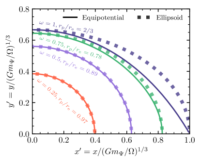
Figure 32: Equipotential lines of the dimensionless Roche potential $\Psi^{\prime}$ given by Equation (36). Solid lines show the equipotentials for which $\omega$ is equal to $0.25,0.5,0.75$ and $1$. Dashed lines show ellipses with the same polar and equatorial radii as the actual equipotentials.

Figure 32 shows how the equipotential surfaces change with increasing $\omega$. For $\omega\lesssim 0.5$ the equipotentials are approximately given by oblate spheroids, while for $\omega$ close to unity a cusp develops at the equator. For this critically rotating surface, the polar radius is $2/3$ of the equatorial one.

By determining the asymptotic behavior of the Roche potential in the limit $\omega\rightarrow 0$, and, when possible, also in the limit $\omega\rightarrow 1$, we have constructed analytic fits to properties of interest. These are described in Appendix B, and include fits for the equatorial radius $r_{\rm e}(r_{\Psi},\omega)$, the centrifugal corrections $f_{P}(\omega)$ and $f_{T}(\omega)$, and the volumes and surface areas of Roche equipotentials, $V_{\Psi}(r_{\rm e},\omega)$ and $S_{\Psi}(r_{\rm e},\omega)$. Previous versions of MESA approximated the specific moment of inertia of isobaric surfaces as that of a thin spherical shell with radius $r_{\Psi}$, $i_{\rm rot}=2r_{\Psi}^{2}/3$, but now default to a fit of the form $i_{\rm rot}(r_{\rm e},\omega)$. Figure 33 shows the resulting fits for $i_{\rm rot}$, $f_{P}$ and $f_{T}$. The new implementation results in values of the specific moment of inertia that are larger by a factor of two as $\omega\rightarrow 1$.

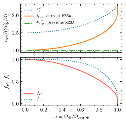
Figure 33: The upper panel shows the specific moment of inertia for a shell of material at different values of $\omega$, normalized by $2/3r_{\Psi}^{2}$. The model implemented previously in MESA is shown with a dot-dashed green line, and the new $\omega$-dependent model for $i_{\rm rot}$ is shown with a solid orange line. As $\omega\rightarrow 1$, the moment of inertia becomes that of a ring with radius $r_{\rm e}$. The lower panel shows the $f_{P}$ and $f_{T}$ factors as a function of $\omega=\Omega/\Omega_{\rm crit}$.

4.2 Implementation in Stellar Evolution Instruments

To include these fits into a stellar evolution calculation that uses the shellular approximation, a value of $\omega$ must be determined for a given specific angular momentum $j_{\rm rot}$, $m_{\Psi}$, and $r_{\Psi}$. From $\Omega_{\Psi}=\omega\Omega_{\rm crit,\Psi}=\omega\sqrt{Gm_{\Psi}/r_{\rm e}^{3}}$ and $j_{\rm rot}=i_{\rm rot}\Omega_{\Psi}$, we find

$$\frac{j_{\rm rot}}{\sqrt{Gm_{\Psi}r_{\Psi}}}=\omega\frac{i_{\rm rot}}{r_{\rm e}^{2}}\sqrt{\frac{r_{\rm e}}{r_{\Psi}}}.$$ (39)

For a given $j_{\rm rot}$, $m_{\Psi}$ and $r_{\Psi}$, the left-hand side can be directly evaluated, while the right-hand side is a monotonic function of $\omega$ for $0\leq\omega\leq 1$. We compute the solution to this equation for each cell in the stellar model using a bisection method. Given $\omega$, we then use the computed fits to determine the values required by the structure equations: $r_{\rm e}$, $r_{\rm p}$, $i_{\rm rot}$, $\Omega_{\Psi}$, $f_{P}$ and $f_{T}$. As in the previous implementation of rotation in MESA, we evaluate these quantities explicitly at the beginning and at the end of a step. The analytical nature of the fits allows the possibility of a fully-coupled and implicit implementation in the future.

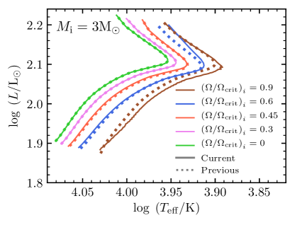
Figure 34: Stellar evolution calculations with initial mass $3\,\mathrm{M}_{\odot}$ and solar metallicity, from ZAMS up to terminal age main sequence (TAMS). Different colors indicate different initial rotation rates, defined in terms of the ratio of the rotational frequency to the critical value at the surface at ZAMS. Solid and dotted lines indicate calculations done with the current and the previous implementations of rotation in MESA, respectively.

Figure 34 shows a $3\,\mathrm{M}_{\odot}$ solar metallicity model with different initial rotational velocities, evolved using the current and previous implementations of rotation in MESA. Both methods agree for rotation rates $\omega<0.5$. Differences at higher rotation rates are due to the aforementioned floor on $f_{P}$ and $f_{T}$. In our current approach we also define a floor on $f_{P}$ and $f_{T}$ in terms of a maximum value $\omega_{\rm max}$, beyond which the effects are truncated to $f_{P}(\omega_{\rm max})$ and $f_{T}(\omega_{\rm max})$. We find that calculations using the new strategy are numerically stable near critical rotation, with the simulations shown in Figure 34 being performed with $\omega_{\rm max}=0.9$. This is in comparison to the previous method, that for rapidly-rotating models set a floor on $f_{P}$ and $f_{T}$ corresponding to their values at $\omega\approx 0.6$. Therefore, MESA can now consistently calculate shellular rotation models closer to critical rotation.

4.3 Gravity Darkening Corrections

Rotating stars are subject to gravity darkening (von Zeipel, 1924a, b). The variation of flux over the surface and the distorted stellar shape imply that the observed properties of the star vary with the angle between the rotation axis of the star and the line of sight (LOS). Here we describe our approach to calculating geometric factors that allow the intrinsic surface quantities $L$ and $T_{\rm eff}$ to be corrected for projection effects along a given LOS. By intrinsic we mean the total $L$ emitted by the star and the $T_{\rm eff}$ associated with this $L$ given the total surface area of the star and the Stefan-Boltzmann law. This is done in two steps. First, we solve the gravity darkening problem for an arbitrary surface element of a rotating star, and second, calculate the projection of the gravity-darkened surface along the LOS.

4.3.1 The Gravity Darkening Model

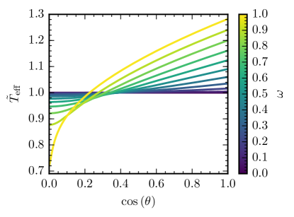
Figure 35: Solution of the ELR model for $0\leq\omega\leq 1$; each curve plots the variation of $\rm{\tilde{T}_{eff}}$ as a function of $\cos(\theta)$ for a different value of $\omega$. Recall that $\cos(\theta)=1$ corresponds to the pole and $\cos(\theta)=0$ to the equator.

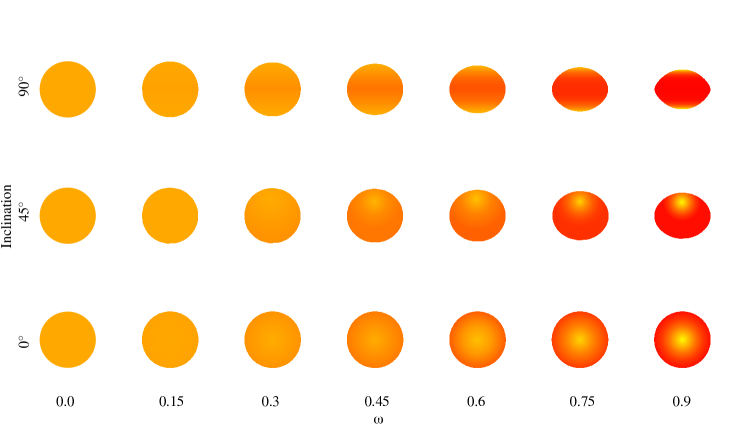
Figure 36: A grid of Roche equipotential surfaces for a range of rotation rates ($\omega$) and inclination angles ($i$). The color of the surface corresponds to the variation in $\tilde{T}_{\rm eff}$ with red corresponding to 0.87 and pale yellow to 1.25; the stars with $\omega=0$ have ${\tilde{T}_{\rm eff}}=1$.

We use the gravity darkening model of Espinosa Lara & Rieutord (2011, hereafter ELR), where it is assumed that the radiative flux is directed antiparallel to the effective surface gravity. At a point on the stellar surface with polar angle $\theta$, we find the value of the scaled photosphere radius $\tilde{r}=R/R_{\rm e}$ by solving

$$\frac{1}{\tilde{r}}+\frac{\omega^{2}}{2}\tilde{r}^{2}\sin^{2}\theta=1+\frac{\omega^{2}}{2}.$$ (40)

We then solve

$$\cos\vartheta+\ln\tan(\vartheta/2)=\frac{1}{3}\omega^{2}\tilde{r}^{3}\cos^{3}\theta+\cos\theta+\ln\tan(\theta/2),$$ (41)

for the modified angular variable $\vartheta$. Using ELR Equation (31), we use this value to obtain the local $T_{\rm eff}$.

Figure 35 shows the variation of $\tilde{T}_{\rm eff}=T_{\rm eff}[L/(4\pi\sigma R_{\rm e}^{2})]^{-1/4}$ over a range of $\theta$ for a series of curves with different values of $\omega$. When $\omega=0$, $\tilde{T}_{\rm eff}=1$ for all $\theta$. When $\omega=1$, $\tilde{T}_{\rm eff}$ varies by nearly a factor of 2 between the pole and the equator.

4.3.2 Projection Effects and Correction Factors

We are interested in the projected—the directional average over the surface along the LOS—$T_{\rm eff}$ and $L$. The two parameters governing the problem are $\omega$ and the inclination angle, $i$, of the LOS with respect to the rotation axis of the star: $i=90^{\circ}$ when the LOS is in the plane of the equator. We denote the LOS unit vector $\hat{l}(i)$ and the projected surface area $\Sigma_{\rm proj}$. Figure 36 shows a grid of Roche equipotential surfaces for different values of $\omega$ and $i$. The color describes the variation of $\tilde{T}_{\rm eff}$ over the surface.

To calculate the luminosity projected along the LOS, $L_{\rm proj}$, requires the surface integral

$$L_{\rm proj}=4\times\iint\limits_{d\vec{\Sigma}\cdot\hat{l}>0}Fd\vec{\Sigma}\cdot\hat{l},$$ (42)

where only the flux projected toward the observer, i.e., $d\vec{\Sigma}\cdot\hat{l}>0$, is kept. The emergent specific intensity from each surface element is assumed to be isotropic. Once $L_{\rm proj}$ and $\Sigma_{\rm proj}$ are known, the projected $T_{\rm eff}$ can be obtained from the Stefan-Boltzmann law

$$T_{\rm eff,proj}=\left(\frac{L_{\rm proj}}{\sigma\Sigma_{\rm proj}}\right)^{1/4}.$$ (43)

As noted by Georgy et al. (2014), the ratio of $L_{\rm proj}/L$, and likewise the ratio of $T_{\rm eff,proj}/T_{\rm eff}$, are geometric factors that depend only on $\omega$ and $i$. We define gravity darkening coefficients

$$C_{L}(\omega,i)\equiv L_{\rm proj}(\omega,i)/L$$ (44)

and

$$C_{T}(\omega,i)\equiv T_{\rm eff,proj}(\omega,i)/T_{\rm eff}.$$ (45)

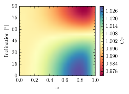
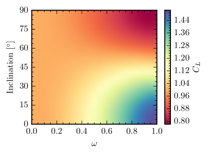
Figure 37: The variation of $C_{T}$ (left panel) and $C_{L}$ (right panel) in the ($\omega,i$)-plane. Note the color scale is different in the two panels.

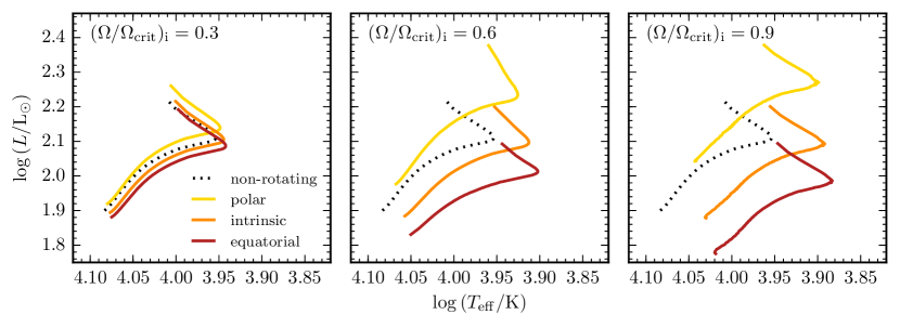
Figure 38: Three rotating tracks from Figure 34 showing the effect of gravity darkening in the HR diagram of a $3\,\mathrm{M}_{\odot}$ model from ZAMS to TAMS. The orange line plots the intrinsic values; the yellow line plots the polar projection; the red line plots the equatorial projection. The dotted line shows the evolution of the non-rotating track.

$C_{T}$ and $C_{L}$ are tabulated in MESA for the valid domain of $\omega$ and $i$; values are readily obtained via bicubic interpolation. The projected $L$ and $T_{\rm eff}$ as viewed from the pole and the equator can be output in the MESA history file; other inclination angles can be accessed via run_star_extras.

Figure 37 shows how $C_{T}$ and $C_{L}$ vary over the ($\omega$,$i$)-plane. These can be compared with the upper panels of Figure 2 in Georgy et al. (2014). The variation of $C_{L}$ is greater than that of $C_{T}$ due to the $\frac{1}{4}$-power relationship between $L$ and $T_{\rm eff}$. At $\omega=1$, where the geometric factors are the largest, $C_{L}$ varies from $-20\%$ to $+50\%$ while $C_{T}$ varies by only about $\pm 2.5\%$.

Figure 37 shows a slight, but noticeable, decrease in $C_{T}$ for $\omega\simeq 1$ whereas the comparable figures from Georgy et al. (2014) do not. When we calculate the coefficients using oblate spheroids instead of Roche equipotential surfaces, we see no such decrease in $C_{T}$ for near-critical rotation.

Figure 38 demonstrates the effect of gravity darkening on 3 of the $3\,\mathrm{M}_{\odot}$ tracks from Figure 34 in the HR diagram. In each panel of Figure 38 the non-rotating track is shown for reference as the dotted line. The magnitude of the gravity darkening effect increases with $\omega$ and is more substantial for $L$ than for $T_{\rm eff}$. Relative to the intrinsic track, the polar projection is brighter and hotter, and the equatorial projection is cooler and fainter.

5 Convective Boundaries and Semiconvection Regions

The correct treatment of convective boundaries continues to be a challenging problem. In this section, we discuss three approaches: the “sign-change” algorithm (Paper I, Paper II), an improved approach called “predictive mixing” (Paper IV), and a new “convective premixing” scheme that addresses several remaining issues.

Early versions of MESA located convective boundaries by searching for sign changes in the discriminant $y$ , defined by $y=y_{\rm S}\equiv\nabla_{{\rm rad}}-\nabla_{{\rm ad}}$ when the Schwarzschild criterion is used to assess convective stability, or by $y=y_{\rm L}\equiv\nabla_{{\rm rad}}-\nabla_{{\rm L}}$ when the Ledoux criterion is used; here $\nabla_{{\rm rad}}$, $\nabla_{{\rm ad}}$ and $\nabla_{{\rm L}}$ are the radiative, adiabatic and Ledoux temperature gradients, respectively. As demonstrated in Paper IV, this sign-change algorithm can fail at convective boundaries that exhibit composition discontinuities. Typically, the failing cases exhibit $\nabla_{{\rm rad}}$ appreciably larger than $\nabla_{{\rm ad}}$ on the convective side of the boundary. Instead, as argued by Gabriel et al. (2014), physical consistency within local mixing length theory (MLT) dictates that $\nabla_{{\rm rad}}=\nabla_{{\rm ad}}$ should hold on the convective side.

In Paper IV we introduced the predictive mixing scheme for treatment of convective boundaries. This scheme improves on the sign-change algorithm by allowing each convection region to expand during a time step until its boundaries satisfy $\nabla_{{\rm rad}}=\nabla_{{\rm ad}}$ on their convective side. The expansion is achieved by modifying convective diffusivities in the cells on the radiative side of a boundary. In Paper IV, we applied predictive mixing in five scenarios: a growing convective core in a $1.5\,\mathrm{M}_{\odot}$ star on the MS; a retreating convective core in a $16\,\mathrm{M}_{\odot}$ star on the MS; growing convective cores in $1\,\mathrm{M}_{\odot}$ and $3\,\mathrm{M}_{\odot}$ stars during the core Helium burning (CHeB) phase; and an evolving convective envelope in a $1\,\mathrm{M}_{\odot}$ star on the MS. Predictive mixing is able to achieve the desired $\nabla_{{\rm rad}}=\nabla_{{\rm ad}}$ outcome in most of these cases.

However, two cases shown in Paper IV continue to exhibit $\nabla_{{\rm rad}}>\nabla_{{\rm ad}}$ on the convective side of a boundary of a convection region, highlighting the need for further work and motivating us to develop a new scheme for treating convective boundaries. This scheme, which we dub “convective premixing”, draws inspiration from earlier work by Castellani et al. (1985) and Mowlavi & Forestini (1994). In the following, we first discuss why predictive mixing sometimes fails. Then, we describe the new convective premixing scheme in detail (Section 5.2), and demonstrate its application in various evolutionary scenarios (Sections 5.3–5.5).

5.1 The Failure of Predictive Mixing

The $16\,\mathrm{M}_{\odot}$ MS scenario presented in Figure 4 of Paper IV exhibits a convective shell above the abundance-gradient region with $\nabla_{{\rm rad}}>\nabla_{{\rm ad}}$ at its lower boundary. If predictive mixing is applied to the shell, the lower boundary advances downward to merge with the core while the upper boundary remains fixed in position. The end result is that the entire abundance-gradient region mixes into the core, delivering significant quantities of fresh H. Such behavior is unphysical, and in Paper IV we made the pragmatic choice to avoid this outcome by disabling predictive mixing for the convective shell.

Additionally, the $1\,\mathrm{M}_{\odot}$ CHeB scenario presented in Figure 6 of Paper IV exhibits $\nabla_{{\rm rad}}>\nabla_{{\rm ad}}$ at the upper boundary of its convective core. This issue cannot be resolved by predictive mixing, as discussed in Paper IV.

In both of these scenarios, the problem encountered is an unavoidable consequence of the design of the predictive mixing scheme, which manipulates the diffusion coefficients at cell faces and then relies on MESA’s abundance solver (Paper I, Section 6.2) to update the model. In contrast, the new convective premixing scheme directly updates the abundances, as we now describe.

5.2 The Convective Premixing Scheme

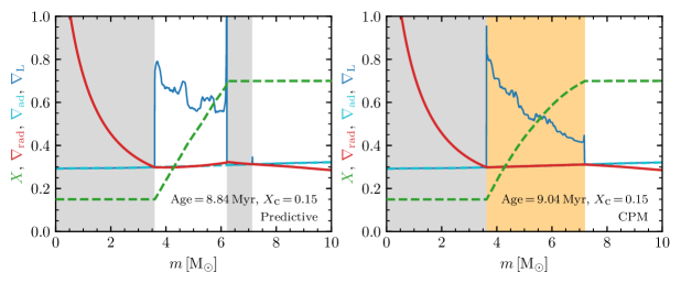
Figure 39: Profiles of $\nabla_{{\rm rad}}$, $\nabla_{{\rm ad}}$, $\nabla_{{\rm L}}$, and $X$ as a function of mass coordinate, in the inner part of the $16\,\mathrm{M}_{\odot}$ MS star at $X_{\rm c}=0.15$. The panels show the separate runs described in the text. Gray (gold) shading indicates convection (semiconvection) regions.

The convective premixing (CPM) scheme is applied at the start of each time step, before any structural or compositional changes that arise due to the evolution of the star. It proceeds by finding the cells where $y>0$ on one face (convective) and $y<0$ on the other face (radiative). For each of these initial boundary cells, the algorithm considers whether $y$ on the radiative face would change if the adjacent cell outside the convection region is mixed completely with the rest of the convection region. This putative mixing is performed at constant cell pressure and temperature, and involves recalculating abundances, densities, opacities and the various temperature gradients ($\nabla_{{\rm rad}}$, $\nabla_{{\rm ad}}$, $\nabla_{{\rm L}}$) throughout the convection region plus the adjacent cell.

If the radiative face of the boundary cell becomes convective during this putative mixing, then the mixing is committed to the model, overwriting the composition profile throughout the entire (newly extended) convection region. Then, the next adjacent cell outside the convection region is considered for incorporation. This process continues iteratively until the radiative face of the current convective boundary remains radiative during the putative mixing.

At a given point in its evolution, a star typically exhibits multiple convective boundaries (for instance, the left panel of Figure 39 shows three). The order in which CPM processes these boundaries is determined by evaluating a characteristic mixing timescale $dr/v_{\rm conv}$ for the initial boundary cells; here, $v_{\rm conv}$ is the convective velocity on the $y>0$ face of the boundary cell, and $dr$ is its radial extent. The boundary with the smallest time scale is processed first, then the boundary with the next-smallest time scale, and so on.

In CPM the mixing is treated as instantaneous. Given that the convective diffusivity $D_{\rm conv}$ is well in excess of $10^{10}\,{\rm cm^{2}s^{-1}}$ even near convective boundaries (see, e.g., Figures 11 and 29 of Paper II), the characteristic mixing timescale is $\tau\sim\Delta r^{2}/D_{\rm conv}\lesssim 10^{4}\,{\rm yr}$ for a typical region with extent $\Delta r\lesssim\mathrm{R}_{\odot}$. This is small compared to typical nuclear timescales, and so the assumption of instantaneous mixing seems warranted for all but the most rapid evolutionary phases.

During its iterations, CPM naturally handles the transition of cell faces inside the convection region from convective to radiative. This typically happens either at the boundary opposite to the advancing one (causing that boundary to retreat), or at a point inside the convection region (causing the region to split). Because mixing through a face ceases when it transitions from convective to radiative, newly-transitioned faces should be very close to convective neutrality. To improve how closely neutrality is achieved, our CPM implementation divides the cell outside the advancing boundary into a number of virtual sub-cells. Each of these sub-cells is mixed into the convective region in turn, until all have been incorporated. The number of sub-cells is automatically adjusted to ensure that, during each sub-cell mix, at most a single face within the current convective region transitions to radiative.

5.3 Evolution of a Retreating Convective Core on the Main Sequence

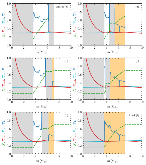
Figure 40: Profiles of $\nabla_{{\rm rad}}$, $\nabla_{{\rm ad}}$, $\nabla_{{\rm L}}$, and $X$ as a function of mass coordinate, in the inner part of the $16\,\mathrm{M}_{\odot}$ MS star at $X_{\rm c}=0.15$. The panels show the outcome of an artificial switch from the predictive mixing scheme to the CPM scheme. The initial state (a) is shown in the upper left panel, and the subsequent panels, running in alphabetical order (b),…,(f), show how this state evolves during the CPM iterations. Gray (gold) shading indicates convection (semiconvection) regions.

We evolve a $16\,\mathrm{M}_{\odot}$ star from the ZAMS to the TAMS. This is the scenario considered in Section 2.3 of Paper IV, and illustrates the behavior of MS stars with retreating convective cores. Here, and for the scenarios presented in the following sections, we assume an initial He mass fraction $Y=0.28$ and an initial metal mass fraction $Z=0.02$, and we ignore rotation and mass loss. Figure 39 plots the profiles of $\nabla_{{\rm rad}}$, $\nabla_{{\rm ad}}$, $\nabla_{{\rm L}}$, and $X$ in the inner parts of the star, at a point nearing the TAMS ($X_{\rm c}=0.15$). The left panel illustrates a run using the predictive mixing scheme applied at the boundary of the convective core, while the right panel shows a run using the CPM scheme; in both calculations, the Ledoux criterion is used to assess convective stability, so that $y=y_{\rm L}$.

In the left panel, the convective shell discussed in Section 5.1 can clearly be seen at the top of the abundance-gradient region, spanning mass coordinates $6.2\lesssim m/\mathrm{M}_{\odot}\lesssim 7.1$. In the right panel, the shell is absent and the abundance-gradient region is wider and shallower, extending all the way out to $m/\mathrm{M}_{\odot}\approx 7.2$. Moreover, the region is very close to adiabatic ($\nabla_{{\rm rad}}=\nabla_{{\rm ad}}$) , in contrast to the super-adiabatic stratification ($\nabla_{{\rm rad}}>\nabla_{{\rm ad}}$) seen in the left panel.

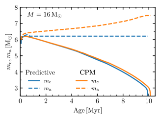
Figure 41: Mass coordinates of the convective core boundary ($m_{\rm c}$) and the top of the abundance-gradient region ($m_{\rm a}$) as a function of MS age, for the 16 $\mathrm{M}_{\odot}$ star. Different line colors show the separate runs discussed in the text.

Schwarzschild & Härm (1958) were the first to predict the appearance of adiabatically stratified abundance-gradient regions outside the convective cores of massive MS stars, labeling them ‘semiconvection regions’. The key feature of a semiconvection region is that the adiabatic stratification is continuously maintained by a gradual adjustment of opacity due to the changing abundance profile.

To illustrate how this adjustment naturally arises within the CPM scheme, we simulate a single evolutionary time step of the $16\,\mathrm{M}_{\odot}$ star where we artificially switch from the predictive scheme to CPM. The starting configuration is the profile shown in the left panel of Figure 39. This panel is reproduced as the upper-left panel of Figure 40; the subsequent panels then show the evolving profiles at selective intermediate stages during the CPM iterations. A clear narrative emerges from these panels: as the lower boundary of the convective shell advances inward, the cell faces near the upper boundary of the shell transition from convective to radiative, causing that boundary to retreat inward. Because there are no abundance gradients within the shell itself, the Ledoux and Schwarzschild criteria give the same condition for this transition to occur: $\nabla_{{\rm rad}}=\nabla_{{\rm ad}}$. The overall effect is that the shell propagates inward as a whole, leaving behind it a ‘wake’ with an adiabatic stratification. Eventually, the propagating shell merges with the core, leading to a final state (seen in the lower-right panel of Figure 40) that closely resembles the right panel of Figure 39 (the small differences are because the former has an evolutionary history determined by the predictive mixing scheme, while the latter has a history determined by CPM).

The seminal paper by Schwarzschild & Härm (1958) triggered significant interest in semiconvection regions, with a particular focus on their final stratification. Sakashita & Hayashi (1961) argued that $y_{\rm L}=0$ should apply in semiconvection regions, rather than $y_{\rm S}=0$ as originally proposed. However, Kato (1966) reasoned that because the former stratification is super-adiabatic ($\nabla_{{\rm rad}}>\nabla_{{\rm ad}}$), slow mixing by overstable g-mode oscillations will drive it toward the same $y_{\rm S}=0$ outcome. Subsequently, Gabriel (1970) suggested that Kato’s mechanism is superfluous, due to the appearance of propagating convective shells that continually adjust the abundance profile to achieve $y_{\rm S}=0$. Gabriel’s narrative closely mirrors the one we give above, and the correspondence between his Figure 1 and our Figure 40 is striking.

A possible source of confusion in this discussion is the relationship between the semiconvection region shown in the right panel of Figure 39, and the semiconvective mixing discussed in Section 4.1 of Paper II. The latter implements the mixing envisaged by Kato (1966); while it will ultimately yield a $y_{\rm S}=0$ stratification, it is a fundamentally different mechanism than the propagating convective shells shown in Figure 40. A critical distinction lies in the role played by the convective stability criterion. While our calculations adopt the Ledoux criterion ($y=y_{\rm L}$), repeating them with the Schwarzschild criterion ($y=y_{\rm S}$) leads to results very similar to the ones already shown (although the abundance profiles are rather more jagged). In contrast, Kato’s mechanism requires the Ledoux criterion to establish an initially super-adiabatic stratification, which the mechanism then drives toward adiabaticity. In hindsight, it seems prudent to reserve the label ‘semiconvection’ for the adiabatically stratified regions envisaged by Schwarzschild & Härm (1958), and avoid using it as in Paper II to describe a mechanism that can generate these regions (for additional examples of this conflation, see e.g., Silva Aguirre et al., 2010; Noels et al., 2010; Ding & Li, 2014; Moore & Garaud, 2016).

To summarize the core and near-core evolution of the $16\,\mathrm{M}_{\odot}$ star, Figure 41 plots the mass coordinate $m_{\rm c}$ of the convective core boundary as a function of MS age for the separate runs using the predictive mixing and CPM schemes. We also show the mass coordinate $m_{\rm a}$ of the top of the abundance-gradient region outside the core; this coincides with the maximal extent of the core in the predictive mixing case, and to the top of the semiconvection region in the CPM case. During the star’s evolution, the opacity change due to progressive H depletion at the center lowers $\nabla_{{\rm rad}}$ throughout the core, causing its boundary to retreat inward. In the CPM case, this retreat is mirrored by an outward growth of the semiconvection region, a behavior first noted by Schwarzschild & Härm (1958). The growth slowly feeds fresh H from the envelope down into the core, which causes the core to shrink slightly less rapidly than in the predictive mixing case, thereby marginally prolonging the star’s MS lifetime.

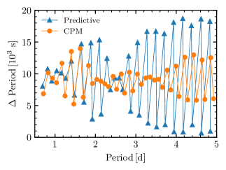
Figure 42: Period spacings $\Delta P$ plotted as a function of period $P$, for $\ell=2$ g-modes of the 16 $\mathrm{M}_{\odot}$ MS star at $X_{\rm c}=0.15$. Different symbols show the separate runs discussed in the text.

As the star nears the TAMS, the mass $m_{\rm a}-m_{\rm c}$ of the abundance-gradient region is $\approx$30% larger in the CPM case than with predictive mixing. This region plays a key role in determining the shape of the Brunt-Väisälä frequency near the core, and the two cases should therefore exhibit differences in their g-mode oscillation spectra. We explore this by using release 5.2 of GYRE (Townsend & Teitler, 2013; Townsend et al., 2018) to evaluate the star’s normal-mode frequencies at $X_{\rm c}=0.15$. Figure 42 plots the resulting period echelle diagram (period $P$ versus period-spacing $\Delta P$) for $\ell=2$ g modes in the period range 0.5–5 d. Both cases show significant departures from the uniform period spacing $\Delta P\approx 10^{4}\,{\rm s}$ predicted by asymptotic theory; these departures are caused by the abundance-gradient region, and therefore are an asteroseismic diagnostic of the star’s age (e.g., Miglio et al., 2008). As the figure shows, the CPM scheme yields significantly smaller non-uniformity in $\Delta P$ for $P\gtrsim 2\,{\rm d}$ than the predictive mixing scheme. These different outcomes are potentially testable by the TESS mission (Ricker et al., 2016), which will observe many massive stars, some with the long time baselines necessary to detect g-modes with multi-day periods. It will first be necessary to explore whether the differences persist when the additional effects of core overshoot and rotation are included.

5.4 Evolution of the Convective Core During Core He Burning

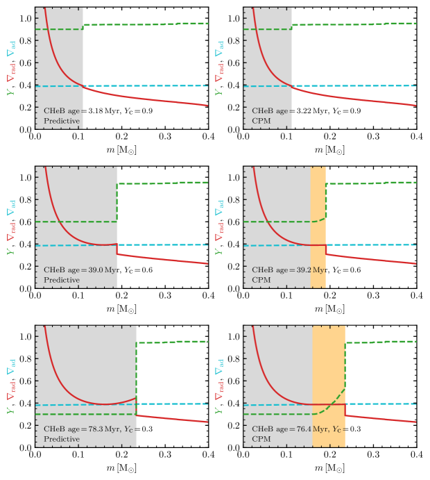
Figure 43: Profiles of $\nabla_{{\rm rad}}$, $\nabla_{{\rm ad}}$, and $Y$ as a function of mass coordinate, in the inner part of the $1\,\mathrm{M}_{\odot}$ star. The panels correspond to different stages during the CHeB phase: $Y_{\rm c}=0.9$ (upper panel), $Y_{\rm c}=0.6$ (middle panel), and $Y_{\rm c}=0.3$ (lower panel). The left panels show the run using the predictive mixing scheme, and the right panels the run using CPM. Gray (gold) shading indicates convection (semiconvection) regions.

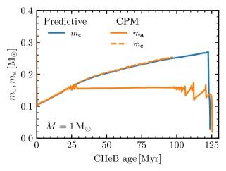
Figure 44: Mass coordinates of the convective core boundary ($m_{\rm c}$) and the top of the abundance-gradient region ($m_{\rm a}$) as a function of CHeB age, for the 1 $\mathrm{M}_{\odot}$ star. Different line colors show the separate runs discussed in the text.

We now evolve a $1\,\mathrm{M}_{\odot}$ star through the CHeB phase; this is the scenario considered in Section 2.4 of Paper IV, and illustrates the behavior of He-burning stars with growing convective cores. Figure 43 plots the profiles of $\nabla_{{\rm rad}}$, $\nabla_{{\rm ad}}$, and $Y$ in the inner parts of the star, at three points during its evolution corresponding to $Y_{\rm c}=0.9$, 0.6 and 0.3. The left panels show a run using the predictive mixing scheme, while the right panels show a run using the CPM scheme; in both calculations, the Ledoux criterion is used to assess convective stability.

The left panels, which reprise Figure 6 of Paper IV, show how a local minimum in $\nabla_{{\rm rad}}$ has developed by $Y_{\rm c}=0.6$. This minimum is held just above the $\nabla_{{\rm ad}}$ threshold using the predictive_superad_thresh control, with the result that the core continues to grow slowly without splitting. With the CPM scheme, a growing semiconvection region develops above a smaller convective core.

The emergence of semiconvection regions during the CHeB phase may have first been proposed by Schwarzschild & Härm (1969), but it was Castellani et al. (1971) and Eggleton (1972) who considered the possibility in detail. Later, Castellani et al. (1985) described a ‘concatenated convective mixings’ scheme for simulating the formation of the semiconvection region; their Figure 3, which can be regarded as a CHeB analog to our Figure 40, reveals how the core splits to form a convective shell, which then propagates outward leaving a wake with an adiabatic stratification. Mowlavi & Forestini (1994) demonstrated how the Castellani et al. (1985) scheme can be generalized to work in other evolutionary phases, and together these two papers provided the original inspiration for the CPM scheme.

To summarize the core and near-core evolution of the $1\,\mathrm{M}_{\odot}$ star, Figure 44 plots the mass coordinate $m_{\rm c}$ of the convective core boundary as a function of CHeB age, for the separate runs using the predictive mixing and CPM schemes. For the CPM run, we also show the mass coordinate $m_{\rm a}$ of the top of the abundance-gradient region outside the core; there is no abundance-gradient region in the predictive mixing run. The figure shows that the semiconvection region forms in the CPM run at an age $\approx 25\,\mathrm{M}\mathrm{yr}$. The top of the semiconvection region then closely tracks the outward growth of the core boundary from the predictive mixing run, through to an age $\approx 95\,\mathrm{M}\mathrm{yr}$. At this juncture, oscillations start to occur in $m_{\rm c}$ for the CPM run. These oscillations are due to breathing pulses, which disrupt the semiconvection region and introduce discontinuities in the abundance profile. Because $m_{\rm a}$ becomes ill-defined when the discontinuities appear, we do not plot it beyond this point. After two final, large-amplitude pulses, the star reaches the end of the CHeB at an age $\approx 125\,\mathrm{M}\mathrm{yr}$, slightly later than the final age for the predictive mixing run.

Debate continues as to whether core breathing pulses during the CHeB phase are physical or numerical (see, e.g., Salaris & Cassisi, 2017, and references therein). In the present context, we note that the instantaneous mixing assumed in the CPM scheme will tend to exacerbate the pulses, because it does not account for the finite time required for He ingested at the top of the semiconvection region to be transported down to the core. We are currently considering improvements that address this shortcoming, but in the meantime we recommend that the CPM scheme be used with caution in the late stages ($Y_{\rm c}\lesssim 0.15$) of the CHeB phase.

5.5 Evolution of a Growing Convective Core on the Main Sequence

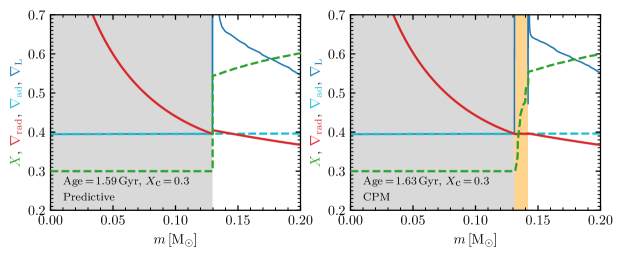
Figure 45: Profiles of $\nabla_{{\rm rad}}$, $\nabla_{{\rm ad}}$, $\nabla_{{\rm L}}$, and $X$ as a function of mass coordinate, in the inner part of the $1.5\,\mathrm{M}_{\odot}$ MS star at $X_{\rm c}=0.30$. The panels show the separate runs described in the text. Gray (gold) shading indicates convection (semiconvection) regions.

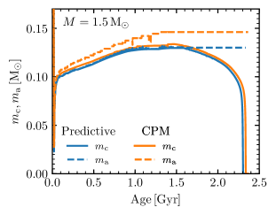
Figure 46: Mass coordinates of the convective core boundary ($m_{\rm c}$) and the top of the abundance-gradient region ($m_{\rm a}$) as a function of MS age, for the 1.5 $\mathrm{M}_{\odot}$ star. Different line colors show the separate runs discussed in the text.

We now evolve a $1.5\,\mathrm{M}_{\odot}$ star from the ZAMS to the TAMS; this is the scenario considered in Section 2.4 of Paper IV, and illustrates the behavior of MS stars with initially growing convective cores. Figure 45 plots the profiles of $\nabla_{{\rm rad}}$, $\nabla_{{\rm ad}}$, $\nabla_{{\rm L}}$ and $X$ in the inner parts of the star when $X_{\rm c}=0.30$. The left panel illustrates a run using the predictive mixing scheme, while the right panel shows a run using the CPM scheme; in both calculations, the Ledoux criterion is used to assess convective stability.

The left panel shows a small super-adiabatic region just outside the core that is stabilized against convection by the abundance gradient ($\nabla_{{\rm ad}}<\nabla_{{\rm rad}}<\nabla_{{\rm L}}$). If slow mixing via the Kato (1966) mechanism were allowed to proceed, this region would eventually transform into a semiconvection region. The right panel shows that the CPM scheme naturally reproduces this semiconvection region. Ledoux (1947) suggests the existence of this semiconvection region (though not labeled as such). The mean molecular weight profile $\mu\propto m\,p^{7/5}$ he obtains for the abundance-gradient region outside the core yields an adiabatic stratification ($\nabla_{{\rm rad}}=\nabla_{{\rm ad}}$).

To bring the present analysis to a close, Figure 46 plots the mass coordinate $m_{\rm c}$ of the convective core boundary as a function of MS age, for the separate $1.5\,\mathrm{M}_{\odot}$ runs using the predictive mixing and CPM schemes. We also show the mass coordinate $m_{\rm a}$ of the top of the abundance-gradient region outside the core. In the predictive mixing case, this region first appears at an age $\approx 1.5\,\mathrm{G}\mathrm{yr}$, when the core boundary reverses direction and begins to retreat inward. In the CPM case, the abundance-gradient region is present from the start, and coincides with the semiconvection region up until an age $\approx 1.75\,\mathrm{G}\mathrm{yr}$. At this point, $\nabla_{{\rm rad}}$ outside the core drops below $\nabla_{{\rm ad}}$, and the semiconvection region becomes radiative; then, without any further ingestion of H from the envelope, $m_{\rm a}$ remains fixed.

6 Parallel Performance

Here we provide updates on the parallel performance of MESAstar. For each test, simulations with different numbers of parallel threads were performed on the same computer with no other CPU-intensive tasks taking place. The tests were performed on one Intel Xeon E5-2699V4 processor with 22 physical cores. Although this processor allows hyperthreading (i.e., two threads running on one physical core), we restrict these tests to one thread per physical core because tests found that enabling hyperthreading results in a performance penalty rather than a benefit.

6.1 Parallel Scaling of MESAstar

MESA uses the OpenMP application programming interface to parallelize certain operations. Among these we distinguish three categories. The first category is operations that are parallel per cell in the stellar model, including the EOS, opacity, and nuclear network. The next category concerns parts of the problem that are a mixture of parallel and serial execution. These include matrix manipulations, the Newton-Raphson solver, and atomic diffusion calculations. The final category is those operations that are serial, such as the main evolve loop and the adjustment of the total mass of the star via mass loss or accretion.

Three MESA test_suite cases are considered: black_hole, 7M_prems_to_agb, and 1M_pre_ms_to_wd. The black_hole test uses 6 structure variables and a nuclear network with 22 isotopes. The 7M_prems_to_AGB test uses 4 structure variables and a nuclear network with 10 isotopes. The 1M_pre_ms_to_wd test uses 4 structure variables and a nuclear network with 8 isotopes and includes rotation.

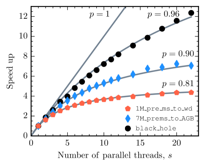
Figure 47: Speed up for the three test cases described in the text when run on different numbers of parallel threads from 1 to 22. Lines are illustrations of Equation (46) for different values of $p$.

As a metric, we define ‘speed up’ to be the ratio of the measured run-time on 1 thread to that on N threads. The theoretical speed up,

$$\frac{1}{(1-p)+(p/s)},$$ (46)

is predicted by Amdahl (1967), where, for our purposes, $s$ is the number of parallel threads and $p$ is the fraction of the code that will benefit from parallel execution for a given test case.

Figure 47 shows the speed up for each of the three cases. In general, we expect cases with more variables (both structure and network) to benefit more from parallel execution. Indeed, the black_hole case shows the best scalability with $p\approx 0.96$, followed by 7M_prems_to_AGB with $p\approx 0.90$, and 1M_pre_ms_to_wd with $p\approx 0.81$. These results are consistent with the numbers of variables included in the respective tests.

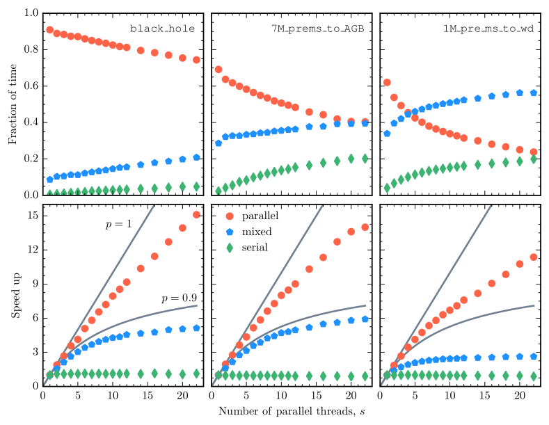
Figure 48: Breakdown of the fraction of the execution time (upper row) and the speed up (lower row) of three different categories listed in the text. Each column is a single test case. The line in the lower panels is Equation (46) for $p=0.9$ and $p=1$.

For each case, Figure 48 shows the relative fraction for the three categories described above and the speed up. The parts of MESAstar that are parallel-per-cell scale nearly linearly with the number of threads while the mixed category scales weakly and the serial component is essentially flat. The serial portion becomes an increasing fraction of the total runtime as the other categories decrease with an increasing number of parallel threads. This may become a greater issue with the move towards many-core processors in the future.

6.2 OP Mono Opacities and Radiative Levitation

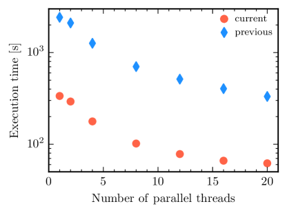
Figure 49: Execution time of the radiative_levitation test suite case. The same test was run using MESA versions before and after the changes described herein to demonstrate the difference in performance obtained by these improvements.

Paper III (Section 9) describes the inclusion of radiative levitation in MESA via the work of Hu et al. (2011). These capabilities were originally developed as part of STARS (Eggleton, 1971; Pols et al., 1995) and evaluate the opacity and radiative acceleration using the OP monochromatic opacity tables (Seaton, 2005). Due to the differing approaches of STARS and MESA, a number of derivatives were being calculated but not used in the MESA implementation of the opacity routines. By eliminating the evaluation of these unused quantities, and by pre-computing some frequently re-used stimulated emission factors, we achieved at least a factor of 5 reduction in the time required to evaluate opacities and radiative accelerations. These optimizations translate into an improvement in total runtime relative to previous versions of MESA when making use of the OP monochromatic opacities or radiative levitation capabilities without any compromise to the numerical results.

We demonstrate in Figure 49 the difference in execution time for runs of the radiative_levitation test suite case using MESA versions before and after the changes described herein. The computational expense of calculating the radiative accelerations continues to dominate the runtime of such models, accounting for more than 65% of run-time even when using 20 parallel threads, meaning these capabilities can benefit from progress toward many-core architectures.

7 Summary

We explain significant new capabilities and improvements implemented in MESA since the publication of Paper I, Paper II, Paper III and Paper IV. The addition of the RSP radial pulsation functionality in MESAstar (Section 2) provides a new capability to model radially-pulsating variable stars. Advances to MESA in numerical energy conservation (Section 3), rotation factors and gravity darkening (Section 4 and Appendix B), and convective boundaries (Section 5), will open opportunities for future investigations in stellar evolution. Improvements in the computational efficiency of MESA on current generation multicore x86 instruction set architectures (Section 6) will inform future development directions. Upgrades to the EOS and nuclear reaction physics (Appendix A) will increase the robustness of stellar evolution models. Discussion of the current treatment of fallback and comparisons of the thermodynamic evolution of supernova models from different software instruments (Appendix C) will enhance the study of massive star explosions. Introduction of the MESA Testhub software infrastructure (Appendix D) for web-based, automated, daily examination of the MESAstar and MESAbinary test suites will lead to more efficient source code development. Input files and related materials for all the figures are available at http://mesastar.org and https://doi.org/10.5281/zenodo.2582656.

Appendix A Updates To Physics Modules

A.1 Equation of State

The EOS is evaluated by the eos module. Figure 50 shows the default coverage in the $\rho-T$ plane. The new PTEH option extends the eos coverage to lower densities (to 10^-18 g cm^-3) and higher metallicities ($Z$ up to 1.0) than allowed by OPAL ($\rho\gtrsim 10^{-10}$ g cm^-3 and $Z$ $\leq$ 0.04 only). Previous versions of eos use HELM to provide approximate results for the low density or $Z>0.04$ cases now covered by PTEH. The PTEH tables are created using the approach of Pols et al. (1995) as implemented by Paxton (2004) in a program derived from Eggleton (1971). PTEH includes a solution to the Saha equations to obtain the dissociation and ionization stages H⁺, H, H₂, He, He⁺, and He⁺⁺ and assumes full ionization of C, N, O, Ne, Mg, Si, and Fe.

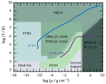
Figure 50: The $\rho-T$ coverage of the EOS used by the eos module. PTEH is from Pols et al. (1995), HELM is from Timmes & Swesty (2000), PC is from Potekhin & Chabrier (2010), OPAL is from Rogers & Nayfonov (2002), SCVH is from Saumon et al. (1995), and the low-density cold region in the lower left is treated as an ideal neutral gas. The region between SCVH and PC is currently problematic from input physics and numerical perspectives and treated as an ideal gas (see Chabrier et al. 2019 for a recent treatment that is not yet in MESA). The blue curve shows the profile of a 25 $\mathrm{M}_{\odot}$ star that has reached an iron core infall speed of 1,000 km s^-1 and the purple curve shows the profile of a 0.8 $\mathrm{M}_{\odot}$ WD.

In addition to PTEH, there are two other new eos options, DT2 and ELM. These are motivated by the need for more numerically accurate partials as discussed in Section 3. In this context, the desired numerical accuracy of the partials is achieved by evaluating analytic partials of the interpolating polynomials rather than by interpolating values of tabulated partials (as is done with OPAL and SCVH data in MESA). As a result, the partials correspond to how the interpolated eos values will actually change in response to small changes of the parameters, whereas interpolated values of partials will be less accurate predictors of the response to such variations. All three new options use bicubic spline interpolation in high resolution tables of $\log(p_{\rm gas}$/erg cm^-3), $\log(e$/erg g^-1), and $\log(s$/erg g${}^{-1}\,\mathrm{K}^{-1}$) to obtain first and second partial derivatives of these quantities with respect to $\log$($\rho$/g cm^-3) and $\log$($T$/$\mathrm{K}$). The options DT2 and ELM use tables holding values derived from OPAL/SCVH and HELM respectively. Figure 51 shows $\nabla_{{\rm ad}}$ in a region of the $\rho-T$ plane covered by DT2 and PTEH.

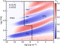
Figure 51: Adiabatic gradient in the $\rho-T$ plane for $X\,=\,0.70$ and $Z\,=\,0.02$. Regions undergoing H₂, H, He, or He⁺ dissociation/ionization are colored blue and labelled. Previous versions of eos truncated the H₂ dissociation region at $\log$($\rho$/g cm^-3)=$-$10, the limit of the SCVH data in eos. Other ionization bands occur at a high enough temperature to be mainly covered by OPAL.

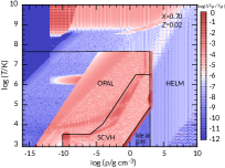
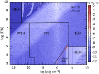
Figure 52: Relative difference in $\chi_{\rho,{\rm gas}}$ between the eos  derivative and a Richardson limit based numerical derivative across the $\rho-T$ plane. The left panel shows the results for the OPAL/SCVH and HELM options, and the right panel shows the results for the PTEH, DT2, and ELM options. Relative differences for the new eos options are $\simeq$ 10^-7, except for a region between SCVH and PC. Note the large difference in accuracy between the old OPAL/SCVH options using interpolated partials and the new DT2 option using partials of interpolating polynomials.

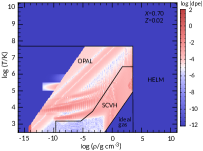
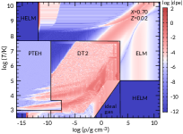
Figure 53: Thermodynamic consistency metric dpe; see Equation (A2) for the definition. The left panel shows the results for OPAL/SCVH and HELM, and the right panel shows the results for PTEH, DT2, and ELM. As expected, HELM gives machine precision consistency and so is superior in this to ELM. OPAL and SCVH have an advantage over DT2 because they use interpolated values of thermodynamically consistent partials $-$ which degrades their numerical accuracy as shown in Figure 52.

A.1.1 Blending

The control structure for blending the various EOS sources in Figure 50 considers a particular source EOS (PTEH, PC, HELM, etc.) to determine what fraction $f$ of the final result comes from that source. A recursive calling structure is used:

level 1

If $f_{\rm PTEH}$=0, then return result of level 2. If $f_{\rm PTEH}$=1, then evaluate PTEH and return. Otherwise, call level 2, blend result with that of PTEH, and return.

level 2

If $f_{\rm PC}$=0, then return result of level 3. If $f_{\rm PC}$=1, then evaluate PC and return result to level 1. Otherwise, call level 3, blend result with that of PC, and return the blended result to level 1.

level 3

If $f_{\rm PTEH,Z}=0$ (i.e., $Z\lesssim$ 0.04), then call level 4 with DT2 and return the result to level 2. If $f_{\rm PTEH,Z}=1$ (i.e., $Z\gtrsim$ 0.04), then call level 4 with PTEH and return the result to level 2. Otherwise (i.e., $Z$ near $0.04$), call level 4 with each of DT2 and PTEH, blend the result in Z and return the blended result to level 2.

level 4

If $f_{\rm PTEH/DT2}$=0, then return result of level 5. If $f_{\rm PTEH/DT2}$=1, then evaluate PTEH/DT2 and return result to level 3. Otherwise, call level 5, blend the result with that of PTEH/DT2 and return the blended result to level 3.

level 5

If $f_{\rm ELM}$=0, then return result of level 6. If $f_{\rm ELM}$=1, then evaluate ELM and return result to level 4. Otherwise, call level 6, blend the result with that of ELM, and return the blended result to level 4.

level 6

Evaluate HELM and return result to level 5.

The blends use a quintic polynomial with zero slope at boundaries. The partial derivatives of the blend polynomial are included in the calculation of the final result to maintain high numerical consistency in the blend region and across EOS region boundaries.

There remain challenges to providing a broad coverage EOS given the current need to combine multiple sources, some of which may not provide the necessary thermodynamic information. For example, when the $\log(\rho$/g cm^-3) blend region extended from 3.0 to 3.1, a negative $\chi_{\rho,{\rm gas}}$ resulted because $\log(p_{\rm gas}$/erg cm^-3) from DT2 were slightly greater than $\log(p_{\rm gas}$/erg cm^-3) from ELM. This could give a drop in $p_{\rm gas}$ as $\log(\rho$/g cm^-3) transitions from DT2 to ELM. Extending the blend region from 2.98 to 3.12 is enough to ensure $\chi_{\rho,{\rm gas}}$ $>$ 0 in the DT2 to ELM transition.

A.1.2 Numerical Accuracy of Partials

To check the numerical accuracy of partials using the new options, we have compared their results with iteratively acquired high precision numerical derivatives (Ridders, 1982; Press et al., 1992). For example, Figure 52 shows the relative difference between the eos  derivative and a Richardson iterative numerical derivative across the $\rho-T$ plane for $\chi_{\rho,{\rm gas}}$. The right panel shows that new options give relative errors of $\simeq$ 10^-7, while the left panel shows that the previous options have larger errors, particularly in the OPAL/SCVH regions. As mentioned in Section 3, those larger errors limit the ability of the MESAstar Newton-Raphson solver to reduce residuals and that in turn can lead to increased errors in numerical energy conservation.

A.1.3 Thermodynamic Consistency

The first law of thermodynamics is an exact differential, which implies

$$p=\rho^{2}\ {\frac{\partial{e}}{\partial{\rho}}}\Biggm{|}_{T,Y_{i}}+T\ {\frac{\partial{p}}{\partial{T}}}\Biggm{|}_{\rho,Y_{i}}\,,\hskip 43.36243pt{\frac{\partial{e}}{\partial{T}}}\Biggm{|}_{\rho,Y_{i}}=T\ {\frac{\partial{s}}{\partial{T}}}\Biggm{|}_{\rho,Y_{i}}\,,\hskip 43.36243pt-{\frac{\partial{s}}{\partial{\rho}}}\Biggm{|}_{T,Y_{i}}=\frac{1}{\rho^{2}}\ {\frac{\partial{p}}{\partial{T}}}\Biggm{|}_{\rho,Y_{i}}\,.$$ (A1)

An EOS is thermodynamically consistent if these relations are satisfied. Thermodynamic inconsistency may manifest itself as an artificial buildup or decay of the entropy during what should be an adiabatic flow. Models that are sensitive to the entropy may suffer inaccuracies if thermodynamic consistency is systematically violated over sufficiently long timescales. Equation (A1) may be recast in a form suitable for evaluating numerical inconsistencies

$$\texttt{dpe}=\frac{\rho^{2}}{p}{\frac{\partial{e}}{\partial{\rho}}}\Biggm{|}_{T,Y_{i}}+\frac{T}{p}{\frac{\partial{p}}{\partial{T}}}\Biggm{|}_{\rho,Y_{i}} -1\,,\qquad\qquad\qquad\qquad\qquad\texttt{dse}=T\left({\frac{\partial{s}}{\partial{T}}}\Biggm{|}_{\rho,Y_{i}}\Bigg{/}{\frac{\partial{e}}{\partial{T}}}\Biggm{|}_{\rho,Y_{i}}\right)-1\,,$$ (A2)

$$\texttt{dsp}=-\rho^{2}\left({\frac{\partial{s}}{\partial{\rho}}}\Biggm{|}_{T,Y_{i}}\Bigg{/}{\frac{\partial{p}}{\partial{T}}}\Biggm{|}_{\rho,Y_{i}}\right)-1\,.$$

Ideally, dpe, dse, and dsp are zero. Figure 53 shows the first thermodynamic consistency quantity, dpe, across the $\rho-T$ plane for an older (MESA r8845) and current version of eos. The other two thermodynamic consistency metrics, dse and dsp, show similar magnitudes. In general, the thermodynamic consistency with DT2 and ELM is reduced relative to the older options directly using OPAL/SCVH and HELM. This is because the thermodynamic consistency relations can only be approximated by bicubic splines. If possible, Hermite interpolation of the Helmholtz free energy would make use of partial derivatives from the EOS and guarantee thermodynamic consistency (e.g., Timmes & Swesty, 2000). However, a bicubic Hermite interpolation produces discontinuities in second derivative quantities (e.g., $\partial{p_{\rm gas}}/\partial{\rho}|_{T,Y_{i}}$) that are problematic for MESA’s Newton-Raphson solver and a biquintic Hermite interpolation requires partial derivatives that are unavailable from some constituents of the EOS patchwork. So for now, we compromise by providing the previous options that give better thermodynamic consistency and the new options that provide better numerical accuracy of partials. The impact of the thermodynamic inconsistencies of the new approach must be evaluated on a case-by-case basis.

A.2 Nuclear Physics

A.2.1 Nuclear Reaction Rates

The Joint Institute for Nuclear Astrophysics (JINA) REACLIB library, which provides the default nuclear reaction rates for MESA, has been updated from the jina_reaclib_results_v2.2 snapshot to the default snapshot. This update includes changes to the fitting formula for a few neutron capture rates that previously returned erroneous values at $T$ $\gtrsim$ 8$\times$10⁹ $\mathrm{K}$. We have modified the default snapshot to include a missing, temperature-independent ${}^{26}\rm{Al}\rightarrow\rm{{}^{26}Mg}$ weak reaction rate. Reaction rates between the ²⁶Al ground and meta-stable states now use Gupta & Meyer (2001). Nuclear partition functions use JINA winvne_v2.0.dat table and JINA masslib_library_5.data provides atomic masses.

A cell’s temperature may exceed $\log(T/\mathrm{K})$ = 10.0 in shocks and explosive burning, which is beyond the range of validity for the fits to the reaction rates and the partition functions. Previously, MESA extrapolated for $\log(T/\mathrm{K})$ $>$ 10.0, leading to erroneous reaction rates. Reaction rates are now set equal to their $\log(T/\mathrm{K})$ = 10.0 values when $\log(T/\mathrm{K})$ $>$ 10.0.

MESA now includes the option to use the electron-capture and $\beta$-decay rates from Suzuki et al. (2016), which cover sd-shell nuclei with $A=17-28$. The primary application for these tables is the evolution of high-density oxygen-neon cores (e.g., Miyaji et al., 1980; Miyaji & Nomoto, 1987; Jones et al., 2013). Compared to the on-the-fly weak rate approach described in Paper III, these tabulated rates are less computationally expensive and more accurate at high temperatures ($T\gtrsim 10^{9}\mathrm{K}$), but less accurate at low temperatures ($T\lesssim 10^{8}\mathrm{K}$) and do not allow explicit updating of nuclear physics.

A.2.2 Reaction Rate Screening

The plasma coupling parameter of two reactants $\Gamma_{i,j}$ and the ion sphere radius $a_{i}$ are

$$\Gamma_{i,j}=\frac{Z_{i}Z_{j}e^{2}}{0.5\left(a_{i}+a_{j}\right)k_{\mathrm{B}}T}\qquad,\qquad a_{i}=\left[\frac{3Z_{i}}{4\pi\left(Z_{i}n_{i}+Z_{j}n_{j}\right)}\right]^{1/3}\,,$$ (A3)

where $Z_{i}$ is the atomic charge of isotope $i$, $e$ is the electron charge, $k_{\mathrm{B}}$ is the Boltzmann constant, and $n_{i}$ is the ion number density of species $i$. MESA applies screening factors to correct nuclear reaction rates for plasma interactions (e.g., Salpeter, 1954). Previous versions defaulted to using one set of expressions for the weak screening regime ($\Gamma_{i,j}$ $\leq$ 0.3, Dewitt et al., 1973; Graboske et al., 1973) and another set of expressions for the strong screening regime ($\Gamma_{i,j}$ $\geq$ 0.8, Alastuey & Jancovici, 1978; Itoh et al., 1979). A linear blend of the weak and strong screening factors is used in the 0.3 $<$ $\Gamma_{i,j}$ $<$ 0.8 intermediate regime. Silicon burning reactions in the cores of massive stars often operate in this intermediate regime. The numerical blending provides a smooth and continuous function that equals the non-blended values and their derivatives at the edges. A new default for screening, based on Chugunov et al. (2007), includes a physical parametrization for the intermediate screening regime and reduces to the familiar weak and strong limits at small and large $\Gamma$ values. We extend the Chugunov et al. (2007) one-component plasma results to a multi-component plasma following Itoh et al. (1979), where the $Z_{i}$ are replaced with the average charge $\bar{Z}$.

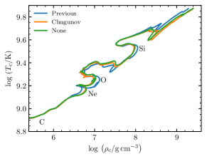
Figure 54: Evolution in the central ($\rho-T$) plane of a 25 $\mathrm{M}_{\odot}$ star until the onset of Fe core-collapse with three different nuclear reaction rate screening options. ‘Previous’ denotes the previous MESA default option, ‘Chugunov’ is the new default option, and ‘None’ applies no screening correction to any nuclear reaction rate. Locations when a fuel undergoes central ignition are labelled.

Figure 54 compares three MESA nuclear reaction rate screening options on the evolution of a 25 $\mathrm{M}_{\odot}$ model. The differences are small from H-burning to the onset of core collapse. However, the Chugunov et al. (2007) implementation takes $\approx 20\%$ fewer time steps, retries, and backups which indicates a numerically smoother solution.

Appendix B Analytical Approximations to the Roche Geometry of a Single Star

In this appendix we compute various properties of the Roche potential of a single star. These are used for the computation of centrifugal effects in stellar structure, as discussed in Section 4. Through these derivations we denote dimensionless properties using an apostrophe, with distances being normalized as $r^{\prime}=r/(Gm_{\Psi}/\Omega^{2})^{1/3}$ and the potential as $\Psi^{\prime}=\Psi/(Gm_{\Psi}\Omega)^{2/3}$.

B.1 Volume of Roche Equipotentials

Following the diagram in Figure 55, the dimensionless volume equivalent radius $r_{\Psi}^{\prime}$ can be computed in terms of $\omega$ as

$$\frac{4}{3}\pi r_{\Psi}^{\prime 3} \equiv V_{\Psi}^{\prime}=2\int_{0}^{\omega^{2/3}}\frac{dV^{\prime}}{dx^{\prime}}dx^{\prime},$$ (B1)

$$\frac{dV^{\prime}}{dx^{\prime}} = 2\pi x^{\prime}y^{\prime},\quad y^{\prime}=\sqrt{\left(\frac{1}{\omega^{2/3}}+\frac{\omega^{4/3}}{2}-\frac{x^{\prime 2}}{2}\right)^{-2}-x^{\prime 2}},$$

where the expression for $y^{\prime}(x^{\prime})$ can be derived directly from the Roche potential. The integral can be solved analytically for the case of $\omega=1$, providing the volume of a critically rotating star in terms of its equatorial radius (Kopal, 1959),

$$V_{\Psi}(\omega=1) = \frac{4\pi}{3}r_{\rm e}^{3}\left[3\sqrt{3}-4+3\ln\left(\frac{3(\sqrt{3}-1)}{\sqrt{3}+1}\right)\right]\simeq\frac{4\pi}{3}\left(0.8149r_{\rm e}\right)^{3}.$$ (B2)

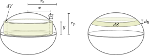
Figure 55: Quantities used for the integration of the $f_{P}$ and $f_{T}$ factors, which require the computation of volume and surface areas of equipotentials.

In the opposite case where $\omega\to 0$, the equipotential is well approximated by an ellipsoid of revolution with

$$r_{\rm p}(\omega)=r_{\rm e}\left(1-\frac{\omega^{2}}{2}+\mathcal{O}(\omega^{4})\right),$$ (B3)

such that its volume is

$$V_{\Psi}(\omega)=\frac{4\pi}{3}r_{\rm e}^{3}\left(1-\frac{\omega^{2}}{2}+\mathcal{O}(\omega^{4})\right).$$ (B4)

By numerically integrating Equation (B1), a simple polynomial approximation to the volume can then be constructed, which is consistent with the value at critical rotation given by Equation (B2) and the asymptotic behaviour at small $\omega$ given by Equation (B4):

$$V_{\Psi}(\omega)\simeq\frac{4\pi}{3}r_{\rm e}^{3}\left(1-\frac{\omega^{2}}{2}+0.1149\omega^{4}-0.07376\omega^{6}\right).$$ (B5)

This expression has an error $<0.25\%$ for $0\leq\omega\leq 1$. In all the asymptotic expressions considered in this work $\omega$ appears in series of even powers, so we do not include odd terms in any fit. Also, since the value for $\omega=1$ is fixed, Equation (B5) is a fit with only 1 free parameter.

Stellar evolution instruments typically use the radial coordinate $r_{\Psi}$, so it is useful to have polynomial fits for $r_{\Psi}(\omega)$ as well. In the limit of $\omega\rightarrow 0$,

$$r_{\Psi}=r_{\rm e}\left(1-\frac{\omega^{2}}{6}+\mathcal{O}(\omega^{4})\right).$$ (B6)

A polynomial fit that matches this and the value at critical rotation $0.8149r_{\rm e}$ from Equation (B2) is

$$r_{\Psi}=r_{\rm e}\left(1-\frac{\omega^{2}}{6}+0.01726\omega^{4}-0.03569\omega^{6}\right),$$ (B7)

which has an error $<0.15\%$ for $0\leq\omega\leq 1$. Similarly, the expression

$$r_{\rm e}=r_{\Psi}\left(1+\frac{\omega^{2}}{6}-0.0002507\omega^{4}+0.06075\omega^{6}\right)$$ (B8)

has an error $<0.2\%$ in the same range.

B.2 Surface Area of Roche Equipotentials

The computation of the dimensionless surface area $S_{\Psi}^{\prime}$ is given by

$$S_{\Psi}^{\prime}=2\int_{0}^{\omega^{2/3}}\frac{dS^{\prime}}{dx^{\prime}}dx^{\prime},\qquad\frac{dS^{\prime}}{dx^{\prime}}=2\pi x^{\prime}\sqrt{\left(\frac{dy^{\prime}}{dx^{\prime}}\right)^{2}+1}.$$ (B9)

In the limit $\omega\rightarrow 0$, $dS^{\prime}/dx^{\prime}$ can be approximated as

$$\frac{dS^{\prime}}{dx^{\prime}}(\omega)=\frac{2\pi x^{\prime}r_{\rm e}^{\prime}}{\sqrt{r_{\rm e}^{\prime 2}-x^{\prime 2}}}\left[1-\frac{1}{2}\left(\frac{x^{\prime}}{r_{\rm e}^{\prime}}\right)^{2}\omega^{2}+\mathcal{O}(\omega^{4})\right],$$ (B10)

which upon integration provides the approximate form of the surface area of a slowly rotating equipotential,

$$S_{\Psi}(\omega)=4\pi r_{e}^{2}\left(1-\frac{\omega^{2}}{3}+\mathcal{O}(\omega^{4})\right).$$ (B11)

This result is consistent with that for an oblate spheroid. Using Equation (B11) and the numerically computed value $S_{\Psi}(\omega=1)=8.832r_{\rm e}^{2}$, a fit to $S_{\Psi}$ that has an error $<0.01\%$ in the range $0<\omega<1$ is

$$S_{\Psi}(\omega)\simeq 4\pi r_{\rm e}^{2}\left(1-\frac{\omega^{2}}{3}+0.08525\omega^{4}-0.04908\omega^{6}\right).$$ (B12)

B.3 Surface Averages of Gravity

The surface average of the dimensionless gravity $\langle g^{\prime}\rangle$ is computed as

$$\langle g^{\prime}\rangle = \frac{2}{S_{\Psi}^{\prime}}\int_{0}^{\omega^{2/3}}g^{\prime}\frac{dS^{\prime}}{dx^{\prime}}dx^{\prime},$$ (B13)

with an equivalent expression for $\langle g^{\prime-1}\rangle$. For reference, the dimensionless gravity is given by ${g^{\prime}=g/(Gm_{\Psi}\Omega^{4})^{1/3}}$. In the limit of $\omega\to 0$, it can be shown that

$$g^{\prime}(\omega)=\frac{1}{r_{\rm e}^{\prime 2}}\left\{1+\left[1-2\left(\frac{x^{\prime}}{r_{\rm e}^{\prime}}\right)^{2}\right]\omega^{2}\right\},$$ (B14)

which combined with Equations (B10) and (B13) results in

$$S_{\Psi}\langle g\rangle=4\pi Gm_{\Psi}\left(1-\frac{2}{3}\omega^{2}+\mathcal{O}(\omega^{4})\right).$$ (B15)

By numerically computing this integral, a simple fit that matches the computed value at $\omega=1$ and has an error $<0.35\%$ for $0\leq\omega\leq 1$ is

$$S_{\Psi}\langle g\rangle=4\pi Gm_{\Psi}\left(1-\frac{2}{3}\omega^{2}+0.3045\omega^{4}+0.001382\omega^{6}\right).$$ (B16)

Similarly the average of the inverse gravity, in the limit of $\omega\to 0$, can be shown to be

$$S_{\Psi}\langle g^{-1}\rangle=\frac{4\pi r_{\rm e}^{4}}{Gm_{\Psi}}\left(1+\mathcal{O}(\omega^{4})\right).$$ (B17)

However, this integral diverges for $\omega=1$, as for a critically rotating star the effective gravity at its equator becomes zero. Although the expression for $S_{\Psi}\langle g^{\prime-1}\rangle$ cannot be integrated in the limit $\omega\rightarrow 1$, by comparing it to the numerical results we have verified that it is approximately given by $S_{\Psi}\langle g^{-1}\rangle\propto-\ln(1-\omega^{4})$. Combining this information with Equation (B17) we have found the following fit with an error $<0.85\%$ in the range $0\leq\omega\leq 0.9999$:

$$S_{\Psi}\langle g^{-1}\rangle=\frac{4\pi r_{\rm e}^{4}}{Gm_{\Psi}}A(\omega),\qquad A(\omega)=1-0.1076\omega^{4}-0.2336\omega^{6}-0.5583\ln(1-\omega^{4}).$$ (B18)

B.4 Moments of Inertia

The specific moment of inertia $i_{\rm rot}$ is needed to determine $\Omega_{\Psi}$ from the specific angular momentum $j_{\rm rot}$ and volume equivalent radius $r_{\Psi}$. To compute $i_{\rm rot}$, consider a shell of material extending from $\Psi$ to $\Psi+d\Psi$. At each point in its surface, its thickness is given by

$$ds=|\nabla\Psi|^{-1}d\Psi=g^{-1}d\Psi.$$ (B19)

Assuming a constant density $\rho$ in the shell (as in the shellular approximation),

$$dm^{\prime} = 2\rho^{\prime}d\Psi^{\prime}\int_{0}^{\omega^{2/3}}g^{\prime-1}\frac{dS^{\prime}}{dx^{\prime}}dx^{\prime}=\rho^{\prime}d\Psi S_{\Psi}^{\prime}\langle g^{\prime-1}\rangle,$$ (B20)

where $dm^{\prime}=dm/m_{\Psi}$ and $\rho^{\prime}=\rho/\left[m_{\Psi}(Gm_{\Psi}/\Omega^{2})^{-3/2}\right]$. From Equation (B20),

$$i_{\rm rot}^{\prime}=\frac{\displaystyle 2\int_{0}^{\omega^{2/3}}x^{2}g^{\prime-1}\frac{dS^{\prime}}{dx^{\prime}}dx^{\prime}}{S_{\Psi}^{\prime}\langle g^{\prime-1}\rangle},$$ (B21)

with the dimensionless specific moment of inertia defined as $i_{\rm rot}^{\prime}=i_{\rm rot}/(Gm_{\Psi}/\Omega^{2})$. Preserving the fit for $S_{\Psi}\langle g^{-1}\rangle$ given by Equation (B18) and using Equations (B10) and (B14), in the limit of $\omega\to 0$

$$i_{\rm rot}(\omega)=\frac{2}{3}r_{\rm e}^{2}\frac{1+\frac{1}{5}\omega^{2}+\mathcal{O}(\omega^{4})}{A(\omega)}.$$ (B22)

Equation (B19) implies that $i_{\rm rot}(\omega=1)=r_{\rm e}^{2}$, as in the extreme of critical rotation $g=0$ at the equator and almost all mass between two close equipotentials lies in a ring of radius $r_{\rm e}^{2}$. Using this information, we construct the following fit which has an error $<0.9\%$ for $0\leq\omega\leq 0.9999$:

$$i_{\rm rot}=\frac{2}{3}r_{\rm e}^{2}\times\frac{B(\omega)}{A(\omega)},\qquad B(\omega)=1+\frac{1}{5}\omega^{2}-0.2735\omega^{4}-0.4327\omega^{6}-\frac{3}{2}\times 0.5583\ln(1-\omega^{4}),$$ (B23)

where the $3/2$ factor in the last term ensures the desired result as $\omega\to 1$.

B.5 Computation of $f_{P}$ And $f_{T}$

Using all the fits constructed so far, $f_{P}$ and $f_{T}$ can be evaluated directly. However, to provide a more compact expression, we keep only the fit for $S_{\Psi}\langle g^{-1}\rangle$ and use Equations (35), (B7) and (B15) to determine the behavior of the remaining terms when $\omega\rightarrow 0$,

$$f_{P}(\omega)=\frac{1-\frac{2}{3}\omega^{2}+\mathcal{O}(\omega^{4})}{A(\omega)},\qquad f_{T}(\omega)=\frac{1+\mathcal{O}(\omega^{4})}{A(\omega)}.$$ (B24)

The following fits for $f_{P}$ and $f_{T}$ are derived, which have errors $<0.8\%$ and $<1.6\%$ in the range $0\leq\omega\leq 0.9999$ respectively:

$$f_{P}(\omega)=\frac{1-\frac{2}{3}\omega^{2}-0.06837\omega^{4}-0.2495\omega^{6}}{A(\omega)},\qquad f_{T}(\omega)=\frac{1+0.2185\omega^{4}-0.1109\omega^{6}}{A(\omega)}.$$ (B25)

B.6 Determination of $\omega$

For given values of $r_{\Psi}$, $m_{\Psi}$, and $j_{\rm rot}$, $\omega$ can be determined from the implicit equation

$$\frac{j_{\rm rot}}{\sqrt{Gm_{\Psi}r_{\Psi}}}=\omega\frac{i_{\rm rot}}{r_{\rm e}^{2}}\sqrt{\frac{r_{\rm e}}{r_{\Psi}}}.$$ (B26)

The left hand side can be directly evaluated, while the right hand side is a monotonic function of $\omega$ for $0\leq\omega\leq 1$.

We compute a fit to the right hand side of Equation (B26). Equations (B6) and (B22) can be used to determine the form of this term in the limit $\omega\rightarrow 0$. In the limit of $\omega\rightarrow 1$ all material is concentrated in a equatorial ring, such that ${j_{\rm rot}(\omega=1)=\sqrt{Gm_{\Psi}r_{\rm e}}}$. Using this information, we find the following fit which has an error $<0.8\%$ in the range $0\leq\omega\leq 0.9999$:

$$\frac{j_{\rm rot}}{\sqrt{Gm_{\Psi}r_{\Psi}}} = \frac{2}{3}\frac{\omega C(\omega)}{A(\omega)},\qquad C(\omega)=1+\frac{17}{60}\omega^{2}-0.3436\omega^{4}-0.4055\omega^{6}-0.9277\ln(1-\omega^{4}).$$ (B27)

This allows the computation of partial derivatives of $\omega$ with respect to $r_{\Psi}$ and $j_{\rm rot}$,

$$\frac{\partial\omega}{\partial r_{\Psi}}=-\frac{3}{4}\frac{j_{\rm rot}}{r^{3/2}\sqrt{Gm_{\Psi}}}\left[\frac{d}{d\omega}\left(\frac{\omega C(\omega)}{A(\omega)}\right)\right]^{-1},\qquad\frac{\partial\omega}{\partial j_{\rm rot}}=\frac{3}{2}\frac{1}{\sqrt{Gm_{\Psi}r_{\Psi}}}\left[\frac{d}{d\omega}\left(\frac{\omega C(\omega)}{A(\omega)}\right)\right]^{-1}.$$ (B28)

Appendix C Core Collapse Supernova Explosions

Paper IV described modeling the evolution of core-collapse supernova (SN) ejecta up to shock breakout with MESA, and with STELLA beyond shock breakout. Modifications since Paper IV have focused on fallback in weak explosions of red supergiant (RSG) stars. In these weak explosions, the total final explosion energy is positive, but insufficient to unbind all material. Thus, some material falls back onto the central object during the subsequent evolution. To quantify and remove this material, we introduce two new user controls. First, we implement a new criterion to select which material is excised from the model during the ejecta evolution. At each time step, MESA calculates the integrated total energy from the innermost cell to cell $j$ above it:

$$E_{j}=\sum_{i={\rm inner}}^{j}\left(e_{i}-\frac{Gm_{i}}{r_{i}}+\frac{1}{2}u_{i}^{2}\right)dm_{i}.$$ (C1)

If $E_{j}<0$, then there is a bound inner region, and MESA continues this sum outward until it reaches a cell $k$ with local positive total energy ($e_{k}-Gm_{k}/r_{k}+u_{k}^{2}/2>0$). MESA removes material inside this cell, making cell $k$ the new innermost cell. Second, to remove any slow-moving, nearly hydrostatic material left near the inner boundary, a minimum innermost velocity can be specified at handoff to STELLA. All material below the innermost cell that has a velocity above this specified velocity is not included in STELLA input files. A velocity cut between 100 - 500 km s^-1 has little effect on light curve properties and the photospheric evolution of Type IIP SNe, and can greatly reduce numerical artifacts that may arise from an inward-propagating shock hitting the inner boundary in STELLA. Such a cut can also lead to a factor of 10 or more reduction in the number of time steps required to produce a light curve. While this scheme is useful in quantifying and excising fallback material, it is not a satisfactory treatment of fallback. For a more complete description of these fallback criteria, see Appendix A of Goldberg et al. (2019).

Next, we look at the evolution of material deep within the ejecta of a Type IIP supernova, at such large optical depths that the outcome is not sensitive to any particular treatment of radiation transport in different software instruments. For this restricted regime, we compare results using MESA+STELLA to quantities derived from the open-source 1D gray radiation hydrodynamics code SNEC (Morozova et al., 2015), both using the same MESA Type IIP ejecta model at shock breakout. This should yield meaningful density and velocity comparisons nearly everywhere in the ejecta and meaningful temperature comparisons very deep within the ejecta.

We explode (with $E_{\rm exp}$ = 10⁵¹ erg) the 99em_19 RSG progenitor model from Paper IV, which has a ZAMS mass of 19 $\mathrm{M}_{\odot}$, and a mass of 17.8 $\mathrm{M}_{\odot}$ and a radius of 603 $\mathrm{R}_{\odot}$ at time of explosion. We excise the inner 1.5 $\mathrm{M}_{\odot}$ and explode the remaining 16.3 $\mathrm{M}_{\odot}$ of ejecta using a thermal bomb as described in Paper IV. The mass of radioactive ${}^{56}{\rm Ni}$ is set to $M_{\rm Ni}$ = 0.03 $\mathrm{M}_{\odot}$. The resulting ejecta is influenced by the inclusion of the Duffell (2016) prescription for mixing due to the Raleigh-Taylor instability in MESA. We then pass our MESA models at shock breakout to both STELLA and SNEC. To mimic the additional line opacities from metals, SNEC employs an opacity floor. We use SNEC’s default opacity floor recommended in Bersten et al. (2011), which is set to $\kappa_{\rm floor,\,core}$ = 0.24 cm² g^-1 for the metal-rich core material, $\kappa_{\rm floor,\,envelope}$ = 0.01 cm² g^-1 for the envelope, and proportional to metallicity for the intermediate region.

Figure 56 shows density and temperature profiles as a function of mass coordinate, with color corresponding to the number of days after shock breakout. Both instruments agree in the density evolution of the expanding ejecta. The temperature evolution is also in agreement in the very optically thick inner ejecta. Temperature differences at the surface reflect the differing treatments of opacity and radiation transfer between SNEC and STELLA.

Figure 57 focuses on the deep core during the first days of the evolution post shock-breakout at the location of the reverse shock generated at the H/He boundary of the initial model. Density, velocity, and temperature profiles over the first 20 days are plotted with the corresponding MESA profile at shock breakout, which serves as the common input in both STELLA and SNEC. By day 20 the reverse shock has reached the inner boundary in both models. Although there are slight differences within the first day, both instruments agree on global properties of the reverse shock and its effects on the temperature and density profiles out to day 20.

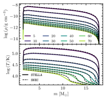
Figure 56: Density (upper panel) and temperature (lower panel) profiles in STELLA (solid colored lines) and SNEC (dashed lines) on the plateau of a Type IIP SN model with $M_{\rm Ni}=0.03\ \mathrm{M}_{\odot}$ at 5 to 70 days after shock breakout in MESA. Lighter colors indicate later days.

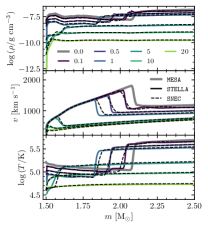
Figure 57: Density (upper panel), velocity (middle panel), and temperature (lower panel) profiles of the 99em_19 progenitor, exploded with $10^{51}$ erg, up to 20 days after shock breakout. The reverse shock originating at the H/He boundary makes its way back through the expanding ejecta. The MESA profile at shock breakout (thick gray line) is used as the input for subsequent evolution in STELLA (solid curves) and SNEC (dashed curves). Numbers in the legend correspond to the day post shock-breakout for each profile.

Appendix D MESA Testhub

Development of the MESA source code is a collaborative process with multiple commits each day from developers working on separate parts of the codebase. In addition to serving as starting templates for science projects, the test cases in MESAstar and MESAbinary exist to detect when changes to the codebase cause unintended deviations from expected behavior (i.e., bugs). The number of test cases grows with time and is currently more than 100, with a total runtime on the order of 10 hours on multicore workstations. Since MESA is committed to supporting reproducibility by giving bit-for-bit identical results on a variety of different hardware and software platforms (Paper III, Section 10), the test suite must be checked on a representative sample of host systems; just as it takes a team to create MESA, it takes a team to test it.

To prevent slowdowns in development that would be caused by running the test suite on multiple hosts before every commit, we have developed the MESA Testhub (testhub.mesastar.org). The Testhub is a web application that collects and organizes the results of test suite submissions via a companion Ruby gem called mesa_test. Every day, submissions from multiple computers and clusters with diverse hardware, operating systems, and compilers check out the most recent revision of MESA, run the test suite, and upload their results to the Testhub. Each day, a summary e-mail is sent to developers detailing which, if any, revisions had failing test cases submitted in the previous 24 hours. With a quick check of the daily email from the Testhub, developers are able to detect cases that fail to give the expected output with bit-for-bit identical results on different computers, or take more than the specified number of time steps, retries, or backups. With daily coverage, we can promptly diagnose issues as soon as they arise by looking at changes from a only handful of commits while maintaining a brisk development pace. The addition of the Testhub has yielded a significant improvement in the pace and quality of MESA development.

References

- Abbott et al. (2017a) Abbott, B. P., Abbott, R., Abbott, T. D., et al. 2017a, Phys. Rev. Lett., 118, 221101, doi: 10.1103/PhysRevLett.118.221101
- Abbott et al. (2017b) —. 2017b, ApJ, 851, L35, doi: 10.3847/2041-8213/aa9f0c
- Abbott et al. (2017c) —. 2017c, Phys. Rev. Lett., 119, 141101, doi: 10.1103/PhysRevLett.119.141101
- Abbott et al. (2017d) —. 2017d, ApJ, 848, L12, doi: 10.3847/2041-8213/aa91c9
- Abbott et al. (2017e) —. 2017e, ApJ, 851, L16, doi: 10.3847/2041-8213/aa9a35
- Abbott et al. (2017f) —. 2017f, ApJ, 850, L40, doi: 10.3847/2041-8213/aa93fc
- Aikawa & Simon (1983) Aikawa, T., & Simon, N. R. 1983, ApJ, 273, 346, doi: 10.1086/161373
- Alastuey & Jancovici (1978) Alastuey, A., & Jancovici, B. 1978, ApJ, 226, 1034, doi: 10.1086/156681
- Alcock et al. (2003) Alcock, C., Alves, D. R., Becker, A., et al. 2003, ApJ, 598, 597, doi: 10.1086/378689
- Amdahl (1967) Amdahl, G. M. 1967, in Proceedings of the April 18-20, 1967, Spring Joint Computer Conference, AFIPS ’67 (Spring) (New York, NY, USA: ACM), 483–485. http://doi.acm.org/10.1145/1465482.1465560
- Artigau et al. (2014) Artigau, É., Sivaramakrishnan, A., Greenbaum, A. Z., et al. 2014, in Society of Photo-Optical Instrumentation Engineers (SPIE) Conference Series, Vol. 9143, Space Telescopes and Instrumentation 2014: Optical, Infrared, and Millimeter Wave, 914340
- Astropy Collaboration et al. (2018) Astropy Collaboration, Price-Whelan, A. M., Sipócz, B. M., et al. 2018, AJ, 156, 123, doi: 10.3847/1538-3881/aabc4f
- Auvergne et al. (2009) Auvergne, M., Bodin, P., Boisnard, L., et al. 2009, A&A, 506, 411, doi: 10.1051/0004-6361/200810860
- Bailer-Jones et al. (2018) Bailer-Jones, C. A. L., Rybizki, J., Fouesneau, M., Mantelet, G., & Andrae, R. 2018, AJ, 156, 58, doi: 10.3847/1538-3881/aacb21
- Ball et al. (2018) Ball, W. H., Chaplin, W. J., Schofield, M., et al. 2018, The Astrophysical Journal Supplement Series, 239, 34, doi: 10.3847/1538-4365/aaedbc
- Beichman et al. (2012) Beichman, C. A., Rieke, M., Eisenstein, D., et al. 2012, in Society of Photo-Optical Instrumentation Engineers (SPIE) Conference Series, Vol. 8442, Space Telescopes and Instrumentation 2012: Optical, Infrared, and Millimeter Wave, 84422N
- Benedict et al. (2002) Benedict, G. F., McArthur, B. E., Fredrick, L. W., et al. 2002, AJ, 123, 473, doi: 10.1086/338087
- Bersten et al. (2011) Bersten, M. C., Benvenuto, O., & Hamuy, M. 2011, ApJ, 729, 61, doi: 10.1088/0004-637X/729/1/61
- Blažko (1907) Blažko, S. 1907, Astronomische Nachrichten, 175, 325, doi: 10.1002/asna.19071752002
- Bono et al. (2000) Bono, G., Marconi, M., & Stellingwerf, R. F. 2000, A&A, 360, 245. https://arxiv.org/abs/astro-ph/0006229
- Bono & Stellingwerf (1994) Bono, G., & Stellingwerf, R. F. 1994, ApJS, 93, 233, doi: 10.1086/192054
- Borucki et al. (2010) Borucki, W. J., Koch, D., Basri, G., et al. 2010, Science, 327, 977, doi: 10.1126/science.1185402
- Breitfelder et al. (2016) Breitfelder, J., Mérand, A., Kervella, P., et al. 2016, A&A, 587, A117, doi: 10.1051/0004-6361/201527030
- Broeg et al. (2013) Broeg, C., Fortier, A., Ehrenreich, D., et al. 2013, in European Physical Journal Web of Conferences, Vol. 47, European Physical Journal Web of Conferences, 03005
- Buchler (2009) Buchler, J. R. 2009, in American Institute of Physics Conference Series, Vol. 1170, American Institute of Physics Conference Series, ed. J. A. Guzik & P. A. Bradley, 51–58
- Buchler et al. (2004) Buchler, J. R., Kolláth, Z., & Cadmus, Jr., R. R. 2004, ApJ, 613, 532, doi: 10.1086/422903
- Buchler et al. (1996) Buchler, J. R., Kollath, Z., Serre, T., & Mattei, J. 1996, ApJ, 462, 489, doi: 10.1086/177167
- Buchler & Kovacs (1987) Buchler, J. R., & Kovacs, G. 1987, ApJ, 320, L57, doi: 10.1086/184976
- Buchler & Moskalik (1992) Buchler, J. R., & Moskalik, P. 1992, ApJ, 391, 736, doi: 10.1086/171384
- Buchler et al. (1990) Buchler, J. R., Moskalik, P., & Kovacs, G. 1990, ApJ, 351, 617, doi: 10.1086/168500
- Byrne & Jeffery (2018) Byrne, C. M., & Jeffery, C. S. 2018, MNRAS, 481, 3810, doi: 10.1093/mnras/sty2545
- Castellani et al. (1985) Castellani, V., Chieffi, A., Tornambe, A., & Pulone, L. 1985, ApJ, 296, 204, doi: 10.1086/163437
- Castellani et al. (1971) Castellani, V., Giannone, P., & Renzini, A. 1971, Ap&SS, 10, 355
- Castor et al. (1977) Castor, J., Davis, Jr., C. G., & Davison, D. K. 1977, , Tech. Rep. LA-6664, TRN: 77-008571, Los Alamos Scientific Lab., NM (USA)
- Chabrier et al. (2019) Chabrier, G., Mazevet, S., & Soubiran, F. 2019, ApJ, 872, 51, doi: 10.3847/1538-4357/aaf99f
- Chandrasekhar (1933) Chandrasekhar, S. 1933, MNRAS, 93, 462, doi: 10.1093/mnras/93.6.462
- Choi et al. (2016) Choi, J., Dotter, A., Conroy, C., et al. 2016, ApJ, 823, 102, doi: 10.3847/0004-637X/823/2/102
- Christensen-Dalsgaard (2008) Christensen-Dalsgaard, J. 2008, Ap&SS, 316, 13, doi: 10.1007/s10509-007-9675-5
- Christy (1964) Christy, R. F. 1964, Reviews of Modern Physics, 36, 555, doi: 10.1103/RevModPhys.36.555
- Chugunov et al. (2007) Chugunov, A. I., Dewitt, H. E., & Yakovlev, D. G. 2007, Phys. Rev. D, 76, 025028, doi: 10.1103/PhysRevD.76.025028
- Clementini et al. (2001) Clementini, G., Federici, L., Corsi, C., et al. 2001, ApJ, 559, L109, doi: 10.1086/323973
- Conroy et al. (2018) Conroy, C., Strader, J., van Dokkum, P., et al. 2018, ApJ, 864, 111, doi: 10.3847/1538-4357/aad460
- Cranmer & Winebarger (2018) Cranmer, S. R., & Winebarger, A. R. 2018, arXiv e-prints, arXiv:1811.00461. https://arxiv.org/abs/1811.00461
- Demarque et al. (2008) Demarque, P., Guenther, D. B., Li, L. H., Mazumdar, A., & Straka, C. W. 2008, Ap&SS, 316, 31, doi: 10.1007/s10509-007-9698-y
- Deming et al. (2009) Deming, D., Seager, S., Winn, J., et al. 2009, Publications of the Astronomical Society of the Pacific, 121, 952, doi: 10.1086/605913
- Dewitt et al. (1973) Dewitt, H. E., Graboske, H. C., & Cooper, M. S. 1973, ApJ, 181, 439, doi: 10.1086/152061
- Ding & Li (2014) Ding, C. Y., & Li, Y. 2014, MNRAS, 438, 1137
- Dorfi & Drury (1987) Dorfi, E. A., & Drury, L. O. 1987, Journal of Computational Physics, 69, 175, doi: 10.1016/0021-9991(87)90161-6
- Dorfi & Feuchtinger (1991) Dorfi, E. A., & Feuchtinger, M. U. 1991, A&A, 249, 417
- Dragomir et al. (2019) Dragomir, D., Teske, J., Günther, M. N., et al. 2019, ApJ, 875, L7, doi: 10.3847/2041-8213/ab12ed
- Duffell (2016) Duffell, P. C. 2016, ApJ, 821, 76, doi: 10.3847/0004-637X/821/2/76
- Eggleton (1971) Eggleton, P. P. 1971, MNRAS, 151, 351
- Eggleton (1972) —. 1972, MNRAS, 156, 361
- Endal & Sofia (1976) Endal, A. S., & Sofia, S. 1976, ApJ, 210, 184, doi: 10.1086/154817
- Espinosa Lara & Rieutord (2011) Espinosa Lara, F., & Rieutord, M. 2011, A&A, 533, A43, doi: 10.1051/0004-6361/201117252
- Faulkner (1968) Faulkner, D. J. 1968, MNRAS, 140, 223, doi: 10.1093/mnras/140.2.223
- Feng et al. (2010) Feng, X., Yang, L., Xiang, C., et al. 2010, ApJ, 723, 300, doi: 10.1088/0004-637X/723/1/300
- Feuchtinger et al. (2000) Feuchtinger, M., Buchler, J. R., & Kolláth, Z. 2000, ApJ, 544, 1056, doi: 10.1086/317260
- Foreman-Mackey et al. (2013) Foreman-Mackey, D., Hogg, D. W., Lang, D., & Goodman, J. 2013, Publications of the Astronomical Society of the Pacific, 125, 306, doi: 10.1086/670067
- Fraley (1968) Fraley, G. S. 1968, Ap&SS, 2, 96, doi: 10.1007/BF00651498
- Freedman et al. (2001) Freedman, W. L., Madore, B. F., Gibson, B. K., et al. 2001, ApJ, 553, 47, doi: 10.1086/320638
- Gabriel (1970) Gabriel, M. 1970, A&A, 6, 124
- Gabriel et al. (2014) Gabriel, M., Noels, A., Montalbán, J., & Miglio, A. 2014, A&A, 569, A63, doi: 10.1051/0004-6361/201423442
- Gaia Collaboration et al. (2018a) Gaia Collaboration, Brown, A. G. A., Vallenari, A., et al. 2018a, A&A, 616, A1, doi: 10.1051/0004-6361/201833051
- Gaia Collaboration et al. (2018b) Gaia Collaboration, Babusiaux, C., van Leeuwen, F., et al. 2018b, A&A, 616, A10, doi: 10.1051/0004-6361/201832843
- Gaia Collaboration et al. (2018c) Gaia Collaboration, Katz, D., Antoja, T., et al. 2018c, A&A, 616, A11, doi: 10.1051/0004-6361/201832865
- Gaidos et al. (2017) Gaidos, E., Kitzmann, D., & Heng, K. 2017, MNRAS, 468, 3418, doi: 10.1093/mnras/stx615
- Gardner et al. (2006) Gardner, J. P., Mather, J. C., Clampin, M., et al. 2006, Space Sci. Rev., 123, 485, doi: 10.1007/s11214-006-8315-7
- Gautschy & Saio (1995) Gautschy, A., & Saio, H. 1995, Annual Review of Astronomy and Astrophysics, 33, 75, doi: 10.1146/annurev.aa.33.090195.000451
- Gautschy & Saio (1996) —. 1996, Annual Review of Astronomy and Astrophysics, 34, 551, doi: 10.1146/annurev.astro.34.1.551
- Georgy et al. (2014) Georgy, C., Granada, A., Ekström, S., et al. 2014, A&A, 566, A21, doi: 10.1051/0004-6361/201423881
- Goldberg et al. (2019) Goldberg, J. A., Bildsten, L., & Paxton, B. 2019, arXiv e-prints, arXiv:1903.09114. https://arxiv.org/abs/1903.09114
- Gombosi et al. (2018) Gombosi, T. I., van der Holst, B., Manchester, W. B., & Sokolov, I. V. 2018, Living Reviews in Solar Physics, 15, 4, doi: 10.1007/s41116-018-0014-4
- Graboske et al. (1973) Graboske, H. C., Dewitt, H. E., Grossman, A. S., & Cooper, M. S. 1973, ApJ, 181, 457, doi: 10.1086/152062
- Gupta & Meyer (2001) Gupta, S. S., & Meyer, B. S. 2001, Phys. Rev. C, 64, 025805, doi: 10.1103/PhysRevC.64.025805
- Hertzsprung (1926a) Hertzsprung, E. 1926a, Bulletin of the Astronomical Institutes of the Netherlands, 3, 115
- Hertzsprung (1926b) —. 1926b, Bull. Astron. Inst. Netherlands, 3, 115
- Hix & Meyer (2006) Hix, W. R., & Meyer, B. S. 2006, Nuclear Physics A, 777, 188, doi: 10.1016/j.nuclphysa.2004.10.009
- Howell et al. (2014) Howell, S. B., Sobeck, C., Haas, M., et al. 2014, Publications of the Astronomical Society of the Pacific, 126, 398, doi: 10.1086/676406
- Hu et al. (2011) Hu, H., Tout, C. A., Glebbeek, E., & Dupret, M.-A. 2011, MNRAS, 418, 195, doi: 10.1111/j.1365-2966.2011.19482.x
- Huang et al. (2018) Huang, C. X., Burt, J., Vanderburg, A., et al. 2018, ApJ, 868, L39, doi: 10.3847/2041-8213/aaef91
- Hunter (2007) Hunter, J. D. 2007, Computing In Science & Engineering, 9, 90
- Itoh et al. (1979) Itoh, N., Totsuji, H., Ichimaru, S., & Dewitt, H. E. 1979, ApJ, 234, 1079, doi: 10.1086/157590
- Jones et al. (2013) Jones, S., Hirschi, R., Nomoto, K., et al. 2013, ApJ, 772, 150, doi: 10.1088/0004-637X/772/2/150
- Kato (1966) Kato, S. 1966, PASJ, 18, 374
- Keller & Wood (2006) Keller, S. C., & Wood, P. R. 2006, ApJ, 642, 834, doi: 10.1086/501115
- Kelly et al. (2018) Kelly, P. L., Diego, J. M., Rodney, S., et al. 2018, Nature Astronomy, 2, 334, doi: 10.1038/s41550-018-0430-3
- Kippenhahn & Thomas (1970) Kippenhahn, R., & Thomas, H.-C. 1970, in IAU Colloq. 4: Stellar Rotation, ed. A. Slettebak, 20
- Klein et al. (2014) Klein, C. R., Richards, J. W., Butler, N. R., & Bloom, J. S. 2014, MNRAS, 440, L96, doi: 10.1093/mnrasl/slu031
- Kluyver et al. (2016) Kluyver, T., Ragan-Kelley, B., Pérez, F., et al. 2016, in Positioning and Power in Academic Publishing: Players, Agents and Agendas: Proceedings of the 20th International Conference on Electronic Publishing, IOS Press, 87
- Kollath et al. (1998) Kollath, Z., Buchler, J. R., Serre, T., & Mattei, J. 1998, A&A, 329, 147
- Kolláth et al. (2002) Kolláth, Z., Buchler, J. R., Szabó, R., & Csubry, Z. 2002, A&A, 385, 932, doi: 10.1051/0004-6361:20020182
- Kopal (1959) Kopal, Z. 1959, Close binary systems (Springer US)
- Kovacs & Buchler (1988) Kovacs, G., & Buchler, J. R. 1988, ApJ, 334, 971, doi: 10.1086/166890
- Kuhfuß (1986) Kuhfuß, R. 1986, A&A, 160, 116
- Leavitt (1908) Leavitt, H. S. 1908, Annals of Harvard College Observatory, 60, 87
- Ledoux (1947) Ledoux, P. 1947, ApJ, 105, 305
- Lindegren et al. (2018) Lindegren, L., Hernández, J., Bombrun, A., et al. 2018, A&A, 616, A2, doi: 10.1051/0004-6361/201832727
- Luri et al. (2018) Luri, X., Brown, A. G. A., Sarro, L. M., et al. 2018, A&A, 616, A9, doi: 10.1051/0004-6361/201832964
- Maeder (2009) Maeder, A. 2009, Physics, Formation and Evolution of Rotating Stars (Springer Berlin Heidelberg), doi: 10.1007/978-3-540-76949-1
- Maeder & Meynet (2000) Maeder, A., & Meynet, G. 2000, Annual Review of Astronomy and Astrophysics, 38, 143, doi: 10.1146/annurev.astro.38.1.143
- Majaess et al. (2009) Majaess, D. J., Turner, D. G., & Lane, D. J. 2009, MNRAS, 398, 263, doi: 10.1111/j.1365-2966.2009.15096.x
- Marconi (2017) Marconi, M. 2017, in European Physical Journal Web of Conferences, Vol. 152, European Physical Journal Web of Conferences, 06001
- Marconi et al. (2013) Marconi, M., Molinaro, R., Bono, G., et al. 2013, ApJ, 768, L6, doi: 10.1088/2041-8205/768/1/L6
- Marconi et al. (2015) Marconi, M., Coppola, G., Bono, G., et al. 2015, ApJ, 808, 50, doi: 10.1088/0004-637X/808/1/50
- McComas et al. (2018) McComas, D. J., Christian, E. R., Schwadron, N. A., et al. 2018, Space Sci. Rev., 214, 116, doi: 10.1007/s11214-018-0550-1
- Meynet & Maeder (1997) Meynet, G., & Maeder, A. 1997, A&A, 321, 465
- Miglio et al. (2008) Miglio, A., Montalbán, J., Noels, A., & Eggenberger, P. 2008, MNRAS, 386, 1487
- Miyaji & Nomoto (1987) Miyaji, S., & Nomoto, K. 1987, ApJ, 318, 307, doi: 10.1086/165368
- Miyaji et al. (1980) Miyaji, S., Nomoto, K., Yokoi, K., & Sugimoto, D. 1980, PASJ, 32, 303
- Moore & Garaud (2016) Moore, K., & Garaud, P. 2016, ApJ, 817, 54
- Morozova et al. (2015) Morozova, V., Piro, A. L., Renzo, M., et al. 2015, ApJ, 814, 63, doi: 10.1088/0004-637X/814/1/63
- Moskalik & Buchler (1990) Moskalik, P., & Buchler, J. R. 1990, ApJ, 355, 590, doi: 10.1086/168792
- Mowlavi & Forestini (1994) Mowlavi, N., & Forestini, M. 1994, A&A, 282, 843
- Muraveva et al. (2018a) Muraveva, T., Delgado, H. E., Clementini, G., Sarro, L. M., & Garofalo, A. 2018a, MNRAS, 481, 1195, doi: 10.1093/mnras/sty2241
- Muraveva et al. (2018b) Muraveva, T., Garofalo, A., Scowcroft, V., et al. 2018b, MNRAS, 480, 4138, doi: 10.1093/mnras/sty1959
- Ness et al. (2015) Ness, M., Hogg, D. W., Rix, H.-W., Ho, A. Y. Q., & Zasowski, G. 2015, ApJ, 808, 16, doi: 10.1088/0004-637X/808/1/16
- Noels et al. (2010) Noels, A., Montalban, J., Miglio, A., Godart, M., & Ventura, P. 2010, Ap&SS, 328, 227
- Papics (2013) Papics, P. I. 2013, PhD thesis, Instituut voor Sterrenkunde, KU Leuven, Celestijnenlaan 200D, B-3001 Leuven, Belgium
- Parker (1958a) Parker, E. N. 1958a, ApJ, 128, 664, doi: 10.1086/146579
- Parker (1958b) —. 1958b, Physics of Fluids, 1, 171, doi: 10.1063/1.1724339
- Paxton (2004) Paxton, B. 2004, PASP, 116, 699, doi: 10.1086/422345
- Paxton et al. (2011) Paxton, B., Bildsten, L., Dotter, A., et al. 2011, ApJS, 192, 3, doi: 10.1088/0067-0049/192/1/3
- Paxton et al. (2013) Paxton, B., Cantiello, M., Arras, P., et al. 2013, ApJS, 208
- Paxton et al. (2015) Paxton, B., Marchant, P., Schwab, J., et al. 2015, ApJS, 220, 15, doi: 10.1088/0067-0049/220/1/15
- Paxton et al. (2018) Paxton, B., Schwab, J., Bauer, E. B., et al. 2018, ApJS, 234, 34, doi: 10.3847/1538-4365/aaa5a8
- Pérez & Granger (2007) Pérez, F., & Granger, B. E. 2007, Computing in Science & Engineering, 9, 21
- Pietrukowicz et al. (2013) Pietrukowicz, P., Dziembowski, W. A., Mróz, P., et al. 2013, Acta Astron., 63, 379. https://arxiv.org/abs/1311.5894
- Pietrukowicz et al. (2017) Pietrukowicz, P., Dziembowski, W. A., Latour, M., et al. 2017, Nature Astronomy, 1, 0166, doi: 10.1038/s41550-017-0166
- Pietrzynski et al. (2012) Pietrzynski, G., Thompson, I. B., Gieren, W., et al. 2012, Nature, 484, 75, doi: 10.1038/nature10966
- Pilecki et al. (2018) Pilecki, B., Gieren, W., Pietrzyński, G., et al. 2018, ApJ, 862, 43, doi: 10.3847/1538-4357/aacb32
- Plachy et al. (2018) Plachy, E., Bódi, A., & Kolláth, Z. 2018, MNRAS, 481, 2986, doi: 10.1093/mnras/sty2511
- Plachy et al. (2013) Plachy, E., Kolláth, Z., & Molnár, L. 2013, MNRAS, 433, 3590, doi: 10.1093/mnras/stt1000
- Pols et al. (1995) Pols, O. R., Tout, C. A., Eggleton, P. P., & Han, Z. 1995, MNRAS, 274, 964, doi: 10.1093/mnras/274.3.964
- Potekhin & Chabrier (2010) Potekhin, A. Y., & Chabrier, G. 2010, Contributions to Plasma Physics, 50, 82, doi: 10.1002/ctpp.201010017
- Press et al. (1992) Press, W. H., Teukolsky, S. A., Vetterling, W. T., & Flannery, B. P. 1992, Numerical recipes in FORTRAN. The art of scientific computing, Vol. 2nd ed. (Cambridge: University Press)
- Reiter et al. (1995) Reiter, J., Walsh, L., & Weiss, A. 1995, MNRAS, 274, 899, doi: 10.1093/mnras/274.3.899
- Richtmyer (1957) Richtmyer, R. 1957, Difference Methods for Initial Value Problems (New York: Interscience)
- Ricker et al. (2016) Ricker, G. R., Vanderspek, R., Winn, J., et al. 2016, in Proc. SPIE, Vol. 9904, Space Telescopes and Instrumentation 2016: Optical, Infrared, and Millimeter Wave, 99042B
- Ridders (1982) Ridders, C. 1982, Advances in Engineering Software (1978), 4, 75 , doi: https://doi.org/10.1016/S0141-1195(82)80057-0
- Rieke et al. (2015) Rieke, G. H., Wright, G. S., Böker, T., et al. 2015, Publications of the Astronomical Society of the Pacific, 127, 584, doi: 10.1086/682252
- Riess et al. (2016) Riess, A. G., Macri, L. M., Hoffmann, S. L., et al. 2016, ApJ, 826, 56, doi: 10.3847/0004-637X/826/1/56
- Riess et al. (2018) Riess, A. G., Casertano, S., Yuan, W., et al. 2018, ApJ, 861, 126, doi: 10.3847/1538-4357/aac82e
- Rogers & Nayfonov (2002) Rogers, F. J., & Nayfonov, A. 2002, ApJ, 576, 1064
- Romero et al. (2018) Romero, A. D., Córsico, A. H., Althaus, L. G., Pelisoli, I., & Kepler, S. O. 2018, MNRAS, 477, L30, doi: 10.1093/mnrasl/sly051
- Roxburgh (2008) Roxburgh, I. W. 2008, Ap&SS, 316, 75, doi: 10.1007/s10509-007-9673-7
- Rydberg et al. (2013) Rydberg, C.-E., Zackrisson, E., Lundqvist, P., & Scott, P. 2013, MNRAS, 429, 3658, doi: 10.1093/mnras/sts653
- Sakashita & Hayashi (1961) Sakashita, S., & Hayashi, C. 1961, Progress of Theoretical Physics, 26, 942
- Salaris & Cassisi (2017) Salaris, M., & Cassisi, S. 2017, Royal Society Open Science, 4, 170192, doi: 10.1098/rsos.170192
- Salpeter (1954) Salpeter, E. E. 1954, Australian Journal of Physics, 7, 373, doi: 10.1071/PH540373
- Saumon et al. (1995) Saumon, D., Chabrier, G., & van Horn, H. M. 1995, ApJS, 99, 713, doi: 10.1086/192204