Membrane stress and torque induced by Frank’s nematic textures: A geometric perspective using surface-based constraints.

Abstract

An elastic membrane with embedded nematic molecules is considered as a model of anisotropic fluid membrane with internal ordering. By considering the geometric coupling between director field and membrane curvature, the nematic texture is shown to induce anisotropic stresses additional to Canham-Helfrich elasticity. Building upon differential geometry, analytical expressions are found for the membrane stress and torque induced by splaying, twisting and bending of the nematic director as described by the Frank energy of liquid crystals. The forces induced by prototypical nematic textures are visualized on the sphere and on cylindrical surfaces.

I Introduction

Nematic textures are intrinsically ordered liquid-crystalline structures expected to induce non-trivial stresses on flexible membranes hel-prost ; kamien ; giomi ; santiago . Their most salient feature is geometric coupling between the nematic order and mechanical stress, which configures the equilibrium distribution of membrane forces. Whereas the curvature elasticity of fluid membranes has been classically approached from the Canham-Helfrich (CH) theory canham ; helfrich ; yang1 ; yang2 ; yang3 , the nematic texture can be modeled by the Frank’s energy considering the distortion modes of splaying, twisting and bending of the nematic director gennes . There is a considerable amount of published work on the structural features of liquid-crystalline membranes both in the theoretical side napoli ; santangelo ; kardar ; nguyen ; aharoni and in experimental setting New2 ; New3 ; New4 , including numerical simulations New4 . The present work adds up mechanical details that remain unexplored from a theoretical point of view, especially regarding extrinsic couplings. By adopting a pure geometric standpoint, we contribute an analytic theory for the anisotropic forces induced by the Frank’s energy of nematic membranes, which outgoes far beyond the well-known geometrical theory of fluid membranes stress ; capo ; fournier . Using the new framework for nematic membranes, the emergence of topological forces between defects could be further analyzed beyond classical approaches nelson ; shin ; santiago ; lopez-leon ; bates . The geometric couplings pointed out configure a counterbalance between membrane elasticity and underlying nematic ordering, which gives rise to the distributions of membrane stresses in dependence with the relative contribution of each material interaction napoli2010 ; vergori ; napoli2016 ; napoli2018 .

In our approach, the connections between membrane curvature and nematic ordering are introduced as geometric constraints to equilibrium forces. Technically, geometric coupling is implemented by exploiting the method of auxiliary variables previously developed in the general context of quadratic constraints to membrane geometry auxiliary ; jemal-book . Specifically, geometrical and compositional constraints accounted for here as Lagrange multipliers contributing to minimize the membrane energy. The curvature-congruent field of membrane stresses is obtained in terms of the Frank’s constants for nematic splay ($\kappa_{1}$), twist ($\kappa_{2}$) and bend ($\kappa_{3}$), which are defined about the global bending rigidity of the membrane ($\kappa$). The description of the resulting curvature-ordering stresses, hereinafter referred to as the Frank-Canham-Helfrich (FCH) field, should enable not only to detail the distribution of membrane forces but also to obtain evolution equations in membrane systems with intrinsic nematic ordering. The geometric interactions here explicited should become in competition with nematic forces, thus determining the particular shape of the flexible membrane, as previously suggested nguyen ; chen-kamien ; mac ; jiang ; seifert . We will focus on the effects imposed by the different Frank’s components on membrane stress and torque, which will be derived for typical nematic textures in the spherical and cylindrical curvature settings. To the best of our knowledge, the geometric theory here approached represent a novelty in the physical description of the mechanics of nematic membranes.

The paper is organized as follows: Section II briefly describes the fundamentals of differential geometry of surfaces that we will be need to later establish our theoretical framework. In Section III the Frank’s energy is presented in terms of the surface director field together with the geometrical constraints imposed on it, which determine the couplings that frame nematic membrane energetics. The specific expressions for stress and torque are presented in Section IV, after detailed calculations in Appendix A using auxiliary variables. In Section V, we introduce the total elastic-nematic stress tensor and the total torque tensor that configurate the core of the mechanical FCH-theory of nematic membranes. In order to visualize the general results in particular cases, we obtain the stress and torque induced by some nematic textures in typical geometric models; in Section VI for the sphere, and in Section VII for the cylinder. In Section VIII, the main results are discussed in the context of the state of the art. Finally, Section IX summarizes the main conclusions.

II Geometry of surfaces

Let us consider the membrane represented by a differentiable surface manifold embedded into the Euclidean space $R^{3}$; this surface is defined by the embedding functions ${\bf X}$, which is parametrized by two internal coordinates $\xi^{a}$, $a=\{1,2\}$ as

$${\bf x}={\bf X}(\xi^{a}),$$ (1)

where the bold denotes the position vector in Cartesian coordinates ${\bf x}=(x^{1},x^{2},x^{3})$ (see Fig. 1).

A local surface basis can be defined as two vector fields tangent to the surface ${\bf e}_{a}=\partial_{a}{\bf X}$, which define the induced metric $g_{ab}={\bf e}_{a}\cdot{\bf e}_{b}$. In addition, $g_{ab}$, and its inverse $g^{ab}$, respectively rises and lowers the tangential indices of surface tensors.

Surface distances. Figure 1 shows the current Riemannian manifold as a metric space where the metric tensor represents the differential distance function; in particular, the length of any tangent vector ${\bf A}=A^{a}{\bf e}_{a}$ is given as ${\bf A}\cdot{\bf A}=|A|^{2}=g_{ab}A^{a}A^{b}$, and the angle $\theta$ between two surface vectors ${\bf A}$ and ${\bf B}$ is determined as $\cos\theta=g_{ab}A^{a}B^{b}/|A||B|$. Because a metric is thus available, any derivative can be directly tied to the shape of the manifold spivak . The Christoffel symbols $\Gamma^{c}_{ab}=\partial_{a}{\bf e}_{b}\cdot{\bf e}^{c}$ provide a representation of the Riemannian connection in terms of surface coordinates. In words, the Christoffel symbols track how the basis changes from point to point; they specify intrinsic derivatives along the tangent vectors of the manifold. Interestingly, the curve connecting two points that has the smallest length is called a geodesic, which fulfills the equation $\ddot{\xi}^{c}+\Gamma_{ab}^{c}\dot{\xi}^{a}\dot{\xi}^{b}=0$ spivak . Other intrinsic concepts, such as intrinsic curvature, parallel transport, etc., can be expressed in terms of Christoffel symbols. In general, the covariant derivative is refereed to as $\nabla_{a}$, in terms of surface coordinates $\xi^{a}$. In addition, the unit normal vector to the surface is defined as ${\bf n}={\bf e}_{1}\times{\bf e}_{2}/\sqrt{g}$ (where $g=\det g_{ab}$), which complements the local basis at any point of the surface.

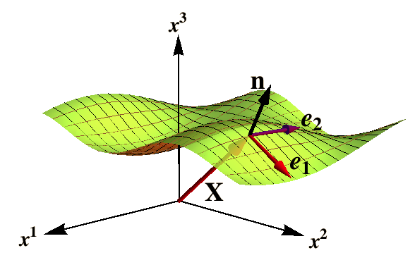
Figure 1: The surface ${\bf x}:=(x^{1},x^{2},x^{3})={\bf X}(\xi^{a})$ embedded into $R^{3}$, the tangent vector fields ${\bf e}_{a}=\partial_{a}{\bf X}$, and the unit normal to the surface ${\bf n}={\bf e}_{1}\times{\bf e}_{2}/\sqrt{g}$; notice that the tangent vector fields may not be orthonormal but ${\bf e}_{a}\cdot{\bf e}_{b}=g_{ab}$.

Surface curvatures. To complete the geometrical description of the surface, we need to define curvatures on the differentiable manifold. Similarly to the metric tensor needed to measure surface distances, a curvature tensor $K_{ab}=-\partial_{a}\partial_{b}{\bf X}\cdot{\bf n}$ is assigned to each point in the Riemannian manifold. Such $K_{ab}$ measures how much the metric tensor is not locally isometric to that of the Euclidean space where the surface is embedded. Consequently, the curvature tensor has to be constructed from second derivatives of the embedding ${\bf X}(\xi^{a})$; this is $K_{ab}=-\partial_{a}{\bf e}_{b}\cdot{\bf n}$. At a given point, second order derivatives are connected with the local curvatures through the Gauss equation:

$$\partial_{a}{\bf e}_{b}=-K_{ab}{\bf n}+\Gamma_{ab}^{c}{\bf e}_{c},$$ (2)

which involves the extrinsic curvature $K_{ab}$, and the Christoffel symbols $\Gamma_{ab}^{c}$, associated with the covariant derivative docarmo . Whereas the normal components in Eq. (2) are said to be extrinsic - as far they cannot be seen by an observer that lives in the surface, the tangential components given by Christoffel symbols are purely intrinsic - since they are only sensed by that internal observer. Notice that, using the covariant derivative, the Gauss equation (2) can be rewritten simply as $\nabla_{a}{\bf e}_{b}=-K_{ab}{\bf n}$.

To specify the geometric connection, let $U^{a}$ to be the tangential components of a surface vector; then, the intrinsic curvature is defined as the commutator of the covariant derivatives as:

$$(\nabla_{a}\nabla_{b}-\nabla_{b}\nabla_{a})U^{c}={\cal R}^{c}{}_{dab}U^{d},$$ (3)

where ${\cal R}_{abcd}=R_{G}(g_{ac}g_{bd}-g_{ad}g_{bc})$ is the Riemann tensor and ${\cal R}_{G}$ the Gaussian curvature of the surface docarmo .

In addition, integrability conditions relate intrinsic and extrinsic curvatures througth the Gauss-Codazzi equation

$$K_{ab}K^{b}{}_{c}=KK_{ac}-g_{ac}{\cal R}_{G},$$ (4)

where $K=g_{ab}K^{ab}$. Finally, the Codazzi-Mainardi equation is given by

$$\nabla_{a}K^{a}{}_{b}=\nabla_{b}K,$$ (5)

which establishes the structure of the Gaussian map that defines the surface.

Surface derivatives. With the covariant derivative $\nabla_{a}$ and the Gauss equation (2), we obtain the covariant derivative of any surface vector field ${\bf A}$, it can be projected in the local basis $\{{\bf e}_{a},{\bf n}\}$ as:

$${\bf A}=A^{a}{\bf e}_{a}+A_{n}{\bf n},$$ (6)

where $A^{a}={\bf A}\cdot{\bf e}^{a}$ and $A_{n}={\bf A}\cdot{\bf n}$. Thus the covariant derivative along the surface can be expressed as:

$$\nabla_{a}{\bf A}=(\nabla_{a}A^{b}+A_{n}K_{a}{}^{b}){\bf e}_{b}+(\nabla_{a}A_{n}-A^{b}K_{ab}){\bf n}.$$ (7)

Noticeably, even the tangential component contains the extrinsic curvature of the surface.

The surface gradient operator is defined as $\nabla={\bf e}^{a}\nabla_{a}$; when operating on a scalar function defined on the surface, we have $\nabla f={\bf e}^{a}\nabla_{a}f={\bf e}^{a}\partial_{a}f$, which is the surface gradient of the function. Using this operator and Eq. (7), the surface divergence $\nabla\cdot{\bf A}$ can be written as aris :

$$\nabla\cdot{\bf A} = {\bf e}^{a}\cdot\nabla_{a}{\bf A},$$ (8)

$$= \nabla_{a}A^{a}+KA_{n},$$

which contains the intrinsic divergence $\nabla_{a}A^{a}$, but also an extrinsic term given as $KA_{n}$. As a matter of fact, using the Gauss equation, the surface divergence of the unit normal is: $\nabla\cdot{\bf n}={\bf e}^{a}\cdot\nabla_{a}{\bf n}=K.$

Likewise, the surface curl operator, defined as $\nabla\times={\bf e}^{a}\nabla_{a}\times$, can be used to obtain

$$\nabla\times{\bf A} = {\bf e}^{a}\times\nabla_{a}{\bf A},$$ (9)

$$= (\nabla_{a}A^{b}+A_{n}K_{a}{}^{b}){\bf e}^{a}\times{\bf e}_{b}$$

$$+ (\nabla_{a}A_{n}-A^{b}K_{ab}){\bf e}^{a}\times{\bf n},$$

$$= \varepsilon^{ab}\nabla_{a}A_{b}\,{\bf n}+(\nabla_{a}A_{n}-A^{b}K_{ab})\varepsilon^{c}{}_{a}{\bf e}_{c},$$

where we have used Eq. (7) and the antisymmetric tensor $\varepsilon_{ab}=\sqrt{g}\epsilon_{ab}$ (with $\epsilon_{ab}$ being Levi-Civita symbols), which defines the normal vector ${\bf e}_{a}\times{\bf e}_{b}=\varepsilon_{ab}{\bf n}$. Note that covariant derivatives can be substituted by partial ones. As shown by Eq. (9), the normal component of the curl vector operation is a geometrically intrinsic term.

Surface nematic director. As shown in Figure 2, we can also define orthonormal vector fields $\boldsymbol{\epsilon}_{\mu}$, $(\mu=1,2)$, tangent to the surface with $\boldsymbol{\epsilon}_{\mu}\cdot\boldsymbol{\epsilon}_{\nu}=\delta_{\mu\nu}$ and ${\bf n}={\boldsymbol{\epsilon}}_{1}\times\boldsymbol{\epsilon}_{2}$. Given a surface vector field $\boldsymbol{\eta}$ we can write it as $\boldsymbol{\eta}=\eta^{a}{\bf e}_{a}$, or equivalently as $\boldsymbol{\eta}=\eta^{\mu}\boldsymbol{\epsilon}_{\mu}$. The director field of the nematic texture is parametrized as a unit vector field:

$$\boldsymbol{\eta}=\cos\Theta\boldsymbol{\epsilon}_{1}+\sin\Theta\boldsymbol{\epsilon}_{2},$$ (10)

where $\Theta$ defines its orientation (see Figure 2) david . Thus, $\eta^{a}=\cos\Theta\,\epsilon_{1}^{a}+\sin\Theta\,\epsilon_{2}^{a}$, for the components, where we used the coefficients $\epsilon_{\mu}^{a}$ that appear into the relationship between the basis; these are $\boldsymbol{\epsilon}_{\mu}=\epsilon_{\mu}^{a}{\bf e}_{a}.$

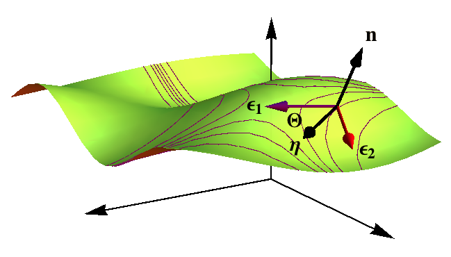
Figure 2: Nematic texture on a curved membrane with director tangent to the surface such that $\boldsymbol{\eta}=\eta^{\alpha}\boldsymbol{\epsilon}_{\alpha}$, where $\boldsymbol{\epsilon}_{\alpha}$ are two unit tangent vector fields such that the unit normal ${\bf n}=\boldsymbol{\epsilon}_{1}\times\boldsymbol{\epsilon}_{2}$. The vector field $\boldsymbol{\eta}_{\perp}$ is defined as $\boldsymbol{\eta}_{\perp}=\boldsymbol{\eta}\times{\bf n}.$

III Surface Frank energy AND GEOMETRIC CONSTRAINTS

For a given texture decorating the surface, the nematic distorsion energy is given by the free Frank’s energy chaikin ,

$$H_{\rm Frank} = \frac{\kappa_{1}}{2}\int dA\,(\nabla\cdot\boldsymbol{\eta})^{2}+\frac{\kappa_{2}}{2}\int dA\,[\boldsymbol{\eta}\cdot(\nabla\times\boldsymbol{\eta})]^{2}$$ (11)

$$+ \frac{\kappa_{3}}{2}\int dA\,[\boldsymbol{\eta}\cdot\nabla)\boldsymbol{\eta}]^{2},$$

where the splay, twist and bend terms are proportional to the respective rigidities ($\kappa_{1}$, $\kappa_{2}$ and $\kappa_{3}$). These components need to be made explicit in terms of the surface derivatives above described. Next, we will discuss separately the meaning of each component.

Splay. The splay energy density involves the surface divergence of the nematic director $\nabla\cdot\boldsymbol{\eta}$, which introduces an energy penalty upon losses of parallel alignment between the elongated molecules chaikin . Assuming that the surface director has no normal component, i.e. $\eta_{n}=0$, using Eq. (8) we can write $\nabla\cdot\boldsymbol{\eta}=\nabla_{a}\eta^{a}.$ Thus, the surface energy due to the splay mode of the nematics is purely intrinsic, i.e. it does not depend on how the surface is embedded in the Euclidean space.

Twist. The twist energy involves the curl operator as describes the energy penalty upon a shear distortion of the nematic alignment. Using the result in Eq. (9) for the surface curl and considering that $\eta_{n}=0$, we can write

$$\nabla\times\boldsymbol{\eta}=(\nabla_{a}\eta^{b})\varepsilon^{a}{}_{b}{\bf n}-\eta^{b}K_{ab}\varepsilon^{ca}{\bf e}_{c}.$$ (12)

Therefore, the term $\boldsymbol{\eta}\cdot\nabla\times\boldsymbol{\eta}=\eta^{b}K_{ab}\eta^{a}_{\perp}$ holds, where the vector field $\eta^{a}_{\perp}=\varepsilon^{ac}\eta_{c}$ has been defined as the tangential (in-plane) transverse component of the director field (see Fig. 2). Unlike the splay, the twist energy does depend on the extrinsic curvature.

Bend. The bend energy density contains the vector field

$$(\boldsymbol{\eta}\cdot\nabla)\boldsymbol{\eta} = \boldsymbol{\eta}\cdot{\bf e}^{a}\nabla_{a}{\eta}$$ (13)

$$= \eta^{a}\nabla_{a}\eta^{b}{\bf e}_{b}-K_{ab}\eta^{a}\eta^{b}{\bf n}.$$

The tangential term (intrinsic) measures the deviation of the nematic director with respect to geodesic curves. Conversely, the normal term is purely extrinsic.

Molecular director: Geometric constraints. Once the Frank energy has been completely explicited as the quadratic moduli of the distortion modes of the molecular director $\boldsymbol{\eta}$ (see Eq. (11)), two geometric constraints are specifically taken into account: i) the nematic field is completely tangent to the surface ($\boldsymbol{\eta}\cdot{\bf n}=0$) ; ii) the nematic director is unitary ($\boldsymbol{\eta}\cdot\boldsymbol{\eta}=1$). Consequently, the total nematic energy:

$$H_{N}=H_{\rm Frank}+\int dA\,\lambda\,\boldsymbol{\eta}\cdot{\bf n}+\frac{1}{2}\int dA\beta\,(\boldsymbol{\eta}\cdot\boldsymbol{\eta}-1),$$ (14)

where $\lambda$ and $\beta$ are Lagrange multipliers that enforce the constraints $\boldsymbol{\eta}\cdot{\bf n}=0$, and $\boldsymbol{\eta}\cdot\boldsymbol{\eta}=1$, respectively. Since both constraints are local in nature, the corresponding Lagrange multipliers are indeed scalar fields defined on the surface. This is because they appear under the integral sign, a formal generalization without practical consequence in the variational evaluation of the equilibrium conditions (see Appendix A). Although this method was originally introduced to examine generalized quadratic curvature constraints auxiliary , in the current context will be exploited to identify the conserved currents associated to the Euclidean invariance of the nematic energy.

IV Nematic Stress and Torque

The nematic stress tensor ${\bf f}^{a}_{\rm Frank}$, appears as a consequence of membrane shape deformations, ${\bf X}\to{\bf X}+\delta{\bf X}$, so that

$$\delta_{\bf X}H_{N}=-\int dA\,{\bf f}^{a}_{\rm Frank}\cdot\nabla_{a}\delta{\bf X}.$$ (15)

After integration by parts, we obtain the main property of the stress tensor as the equilibrium condition; namely, its covariant conservation, $\nabla_{a}{\bf f}^{a}_{\rm Frank}=0$. The explicit calculation of the stress tensor has been presented in the Appendix A, where we have found the expression for the Lagrange multiplier

$$-\lambda = {\kappa}_{1}\nabla_{a}\eta^{a}K+{\kappa}_{2}(2K_{\tau}\nabla_{a}\eta^{a}_{\perp}+\eta^{a}_{\perp}\nabla_{a}K_{\tau})$$ (16)

$$+\kappa_{3}[\nabla_{b}\eta^{b}K_{\eta}+\eta^{b}\nabla_{b}\eta^{a}K_{ad}\eta^{d}$$

$$+\eta^{b}\eta^{c}(\nabla_{c}\eta^{d}K_{bd}+\nabla_{b}K_{cd}\eta^{d}+K_{cd}\nabla_{b}\eta^{d})],$$

where $K_{\tau}=K_{ab}\eta^{a}_{\perp}\eta^{b}$. The multiplier $\lambda$ enforces the nematic director to be tangent to the surface. In fact, $\lambda$ contributes to the normal force per unit length on the membrane, as we will see below. Likewise, the multiplier $\beta$ does not play role in the stress tensor (see Appendix A).

Therefore, the splay stress tensor is found to be:

$$\frac{{\bf f}^{a}_{S}}{\kappa_{1}} = \nabla_{d}\eta^{d}\left(\nabla^{c}\eta^{a}-\frac{g^{ac}}{2}\nabla_{d}\eta^{d}\right){\bf e}_{c}$$ (17)

$$- \nabla_{c}\eta^{c}(K\eta^{a}-K^{a}{}_{c}\eta^{c}){\bf n},$$

where the tangential components contain intrinsic information of the surface through $g_{ab}$ and covariant derivatives of $\eta^{a}$; the normal component includes, instead, coupling with extrinsic curvature. Note that both components are proportional to the divergence of the nematic director, so that in the case of textures without sources and sinks, the splay stress vanishes.

The force per unit length, on a surface curve with unit tangent ${\bf T}=T^{a}{\bf e}_{a}$, and conormal ${\bf l}=l^{a}{\bf e}_{a}$ (see Fig.3), is calculated by projecting the stress tensor as deserno :

$${\bf f}^{a}_{S}l_{a}=F_{T}^{S}{\bf T}+F_{l}^{S}{\bf l}+F_{n}^{S}{\bf n},$$ (18)

where the projections are given by

$$F_{T}^{S} = \kappa_{1}\nabla_{d}\eta^{d}T^{c}l^{a}\nabla_{c}\eta_{a},$$

$$F_{l}^{S} = \kappa_{1}\nabla_{d}\eta^{d}\left(l^{a}l^{c}\nabla_{c}\eta_{a}-\frac{1}{2}\nabla_{b}\eta^{b}\right),$$

$$F_{n}^{S} = -\kappa_{1}\nabla_{d}\eta^{d}(K\eta_{a}l^{a}-K_{ab}l^{a}\eta^{b}).$$ (19)

When considering the twist term of the Frank’s energy, using the same method of auxiliary variables (see Appendix A), the calculated twist stress tensor is

$$\frac{{\bf f}_{W}^{a}}{\kappa_{2}} = K_{\tau}(K^{cb}\eta_{c}\eta_{\perp}^{a}-\frac{g^{ab}}{2}K_{\tau}){\bf e}_{b}$$ (20)

$$- [(2K_{\tau}\nabla_{c}\eta^{c}_{\perp}+\eta^{c}_{\perp}\nabla_{c}K_{\tau})\eta^{a}$$

$$+ K_{\tau}\eta_{\perp c}\nabla^{a}\eta^{c}]{\bf n},$$

where all the terms have coupling with extrinsic curvature. In this case, we found:

$$F_{T}^{W} = \kappa_{2}K_{\tau}K_{cb}\eta^{c}T^{b}\eta_{\perp}^{a}l_{a},$$

$$F_{l}^{W} = \kappa_{2}K_{\tau}\left(K_{cb}\eta^{c}l^{b}\eta_{\perp}^{a}l_{a}-\frac{K_{\tau}}{2}\right),$$

$$F_{n}^{W} = -\kappa_{2}[(2K_{\tau}\nabla_{c}\eta^{c}_{\perp}+\eta^{c}_{\perp}\nabla_{c}K_{\tau})\eta^{a}l_{a}$$ (21)

$$+ K_{\tau}\eta_{\perp c}l^{a}\nabla_{a}\eta^{c}].$$

Finally, the bend stress tensor obtained is:

$$\frac{{\bf f}_{B}^{a}}{\kappa_{3}} = \Big{[}K_{\eta}\eta^{c}\eta^{a}K^{b}{}_{c}+\eta^{a}\eta^{d}\nabla_{d}\eta^{c}\nabla^{b}\eta_{c}$$ (22)

$$- \frac{g^{ab}}{2}(\eta^{d}\eta^{e}\nabla_{d}\eta^{c}\nabla_{e}\eta_{c}+K_{\eta}^{2})\Big{]}{\bf e}_{b}$$

$$- \Big{[}\nabla_{b}\eta^{b}K_{\eta}+3\eta^{b}\nabla_{b}\eta^{c}K_{cd}\eta^{d}$$

$$+ \eta^{b}\eta^{c}\eta^{d}\nabla_{b}K_{cd}\Big{]}\eta^{a}{\bf n},$$

with the projections

$$F_{T}^{B} = \kappa_{3}[K_{\eta}K_{bc}T^{b}\eta^{c}+\eta^{d}\nabla_{d}\eta^{c}T^{b}\nabla_{b}\eta_{c}]\eta^{a}l_{a},$$

$$F_{l}^{B} = \kappa_{3}[K_{\eta}K_{bc}l^{b}\eta^{c}+\eta^{d}\nabla_{d}\eta^{c}l^{b}\nabla_{b}\eta_{c}]\eta^{a}l_{a}$$

$$- \frac{\kappa_{3}}{2}\left(\eta^{d}\eta^{e}\nabla_{d}\eta^{c}\nabla_{e}\eta_{c}+K_{\eta}^{2}\right),$$

$$F_{n}^{B} = -\kappa_{3}\Big{[}\nabla_{b}\eta^{b}K_{\eta}+3\eta^{b}\nabla_{b}\eta^{c}K_{cd}\eta^{d}$$ (23)

$$+ \eta^{b}\eta^{c}\eta^{d}\nabla_{b}K_{cd}\Big{]}\eta^{a}l_{a},$$

Total nematic force. Because the energy is additive, we get the total stress of the nematic membrane as:

$${\bf f}^{a}_{\rm Frank}={\bf f}^{a}_{S}+{\bf f}^{a}_{W}+{\bf f}^{a}_{B}.$$ (24)

The analytic outcome in Eqs. (17)-(23), is the most relevant result of this paper. As far as we know, this result had not been presented before; it establishes explicit relationships for the tensor components of the membrane stress due to the presence of the nematics.

Once we have described the stress tensor, let’s look at the consequences of translations and rotations in the energy. Let us notice that when the equilibrium condition is satisfied, the variation of the energy can be written as

$$\delta H_{N} = -\int dA\nabla_{a}({\bf f}^{a}_{\rm Frank}\cdot\delta{\bf X})-\int dA\nabla_{a}(\Lambda^{ab}{\bf e}_{a}\cdot\delta{\bf n})$$ (25)

$$+ \int dA\nabla_{a}({\cal H}^{a}\cdot\delta\boldsymbol{\eta}),$$

where we have defined

$${\cal H}^{a}=\kappa_{1}(\nabla_{b}\eta^{b}){\bf e}^{a}+\kappa_{2}K_{\tau}(\boldsymbol{\eta}\times{\bf e}^{a})+\kappa_{3}\eta^{a}(\eta^{b}\nabla_{b}\boldsymbol{\eta}),$$ (26)

and $\Lambda^{ab}=-\partial H_{\rm Frank}/\partial K_{ab}$ (see appendix A).

Translations. Let us consider first an infinitesimal translation of the surface element $\delta{\bf X}={\bf a}$. Deformation of the tangent vectors can be found, $\delta{\bf e}_{a}=\partial_{a}\delta{\bf X}=0$, thus $\delta{\bf n}=0$, and similarly $\delta\boldsymbol{\eta}=0$. Consequently,

$$\delta H_{N}=-{\bf a}\cdot\oint_{\cal C}ds\,{\bf f}^{a}_{\rm Frank}l_{a},$$ (27)

and as we mentioned above, ${\bf f}^{a}_{\rm Frank}l_{a}$ is identified as the force, per unit length, acting on the loop $\cal C$. The line integral in the right hand of Eq. (27) is the generalized force exerted by a surface element decorated with the nematics; otherwise said, it holds for the contribution to membrane tension arising from the nematic texture. This is how translation symmetry give rise to the membrane stress tensor, with the surface tension being the conserved quantity related to this continuos symmetry of the membrane.

Rotations. Let us consider now an infinitesimal rotation of the shape membrane, $\delta{\bf X}=\boldsymbol{\omega}\times{\bf X}$. The unit normal undergoes a rotation, $\delta{\bf n}=\boldsymbol{\omega}\times{\bf n}$, and the nematic director changes as $\delta\boldsymbol{\eta}=-(\boldsymbol{\eta}\cdot\delta{\bf n})\,{\bf n}$. Consequently, under an infinitesimal rotation, the energy deformation can be written as

$$\delta H_{N} = -\boldsymbol{\omega}\cdot\int dA\nabla_{a}{\bf M}^{a}_{\rm Frank},$$ (28)

$$= -\boldsymbol{\omega}\cdot\oint_{\cal C}ds\,{\bf M}^{a}_{\rm Frank}l_{a},$$

where the nematic torque is defined as

$${\bf M}^{a}_{\rm Frank}={\bf X}\times{\bf f}^{a}_{\rm Frank}+{\bf m}^{a}_{\rm Frank},$$ (29)

and

$${\bf m}^{a}_{\rm Frank}=(\kappa_{2}K_{\tau}\eta_{\perp}^{a}+\kappa_{3}K_{\eta}\eta^{a})\boldsymbol{\eta}_{\perp}.$$ (30)

The first term in Eq. (29) is the external nematic torque, induced by the Frank energy; the second one is identified as the intrinsic nematic torque, a vector field that points in direction $\boldsymbol{\eta}_{\perp}$, the rotational axis. We notice that the splay energy does not induce intrinsic torque, this is because under rotations, the nematic director deforms in a normal direction to the surface. The nematic torque here obtained is the second foremost result of this paper.

V Total elastic-nematic stress and torque

After calculating the nematic components to the stress tensor, contributions from surface elasticity must be properly casted to account for the total membrane stress; the complete free energy is given by

$$H = H_{N}+H_{\rm CH},$$ (31)

where the Canham-Helfrich (CH) energy holds

$$H_{\rm CH}=\frac{\kappa}{2}\int dA(K-K_{0})^{2}+\sigma\int dA.$$ (32)

This functional accounts for the flexural elasticity and the lateral tension of fluid membranes, which can be described in terms of surface geometry through the bending rigidity $\kappa$, the spontaneous curvature $K_{0}$, and the membrane tension $\sigma$ seifert . After minimization $\delta F_{\rm CH}=0$, the CH stress tensor, can be written as deserno :

$${\bf f}^{a}_{\rm CH} = \Big{\{}\kappa(K-K_{0})[K^{ab}-\frac{1}{2}(K-K_{0})g^{ab}]-\sigma g^{ab}\Big{\}}{\bf e}_{b}$$ (33)

$$- \kappa(\nabla^{a}K){\bf n}.$$

By taking this result into account, the total stress tensor of the nematic membrane energetically described by Eq. (31) is thus ${\bf f}^{a}={\bf f}^{a}_{\rm Frank}+{\bf f}^{a}_{\rm CH}$. For a closed membrane, namely, a vesicle, the pressure difference $P$ between the outer medium and the vesicle interior imposes that the stress tensor is not conserved but

$$\nabla_{a}{\bf f}^{a}=P{\bf n}.$$ (34)

When integrating Eq. (34) over the area of the patch ${\cal M}$ with boundary the loop ${\cal C}$, parametrized by arc length $s$, as showed in Figure 3, we have

$$\oint_{\cal C}ds\,{\bf f}^{a}l_{a} = P\int_{\cal M}\,dA\,{\bf n},$$ (35)

$$= \frac{P}{2}\oint_{\cal C}\,ds\,{\bf X}\times{\bf T}.$$

Let’s notice that this equation sets down a counterbalance between the compositional stress due to the nematics and the elastic stress due to bending stiffness, membrane tension and external pressure.

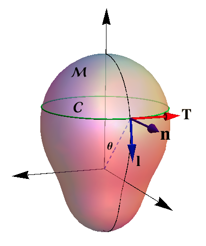
Figure 3: The Darboux frame adapted to the curve $\cal C$ docarmo : $\bf T$ the unit tangent, $\bf n$ the unit normal to the surface and the conormal ${\bf l}={\bf T}\times{\bf n}$. We can be expand along the tangent basis to the surface as ${\bf T}=T^{a}{\bf e}_{a}$, and ${\bf l}=l^{a}{\bf e}_{a}$, so that $T^{a}T_{a}=1=l^{a}l_{a}$ and $T^{a}l_{a}=0$. The induced metric can then be written as $g_{ab}=T_{a}T_{b}+l_{a}l_{b}$.

Because the force that the nematic contained in region $\cal M$ exerts on the loop $\cal C$ is given by

$${\bf F}_{\rm Frank}=\oint_{\cal C}ds\,{\bf f}^{a}_{\rm Frank}l_{a},$$ (36)

where the nematic force, per unit length, is

$${\bf f}^{a}_{\rm Frank}l_{a} = ({\bf f}^{a}_{S}+{\bf f}^{a}_{W}+{\bf f}^{a}_{B})l_{a},$$ (37)

$$= F_{T}^{\rm Frank}{\bf T}+F_{l}^{\rm Frank}{\bf l}+F_{n}^{\rm Frank}{\bf n},$$

and $F_{T}^{\rm Frank}=F_{T}^{S}+F_{T}^{W}+F_{T}^{B}$; similarly for $F_{l}^{\rm Frank}$ and $F_{n}^{\rm Frank}$.
In order to account for the equilibrium tradeoff between ordering interactions and membrane elasticity, the nematic force have to be completed with the elastic force given by fournier ; deserno

$$F_{n}^{\rm CH} = -\kappa\nabla_{l}K,$$

$$F_{l}^{\rm CH} = -\Sigma+\frac{\kappa}{2}[K_{l}^{2}-K_{T}^{2}+2K_{T}K_{0}],$$

$$F_{T}^{\rm CH} = \kappa(K-K_{0})K_{lT},$$ (38)

where the effective membrane tension $\Sigma=\sigma+\kappa K_{0}^{2}/2$, $K_{l}=K_{ab}l^{a}l^{b}$, $K_{T}=K_{ab}T^{a}T^{b}$, $K_{lT}=K_{ab}l^{a}T^{b}$ and $\nabla_{l}K=\l^{a}\nabla_{a}K$.

Furthermore, the total torque can be written as

$${\bf M}^{a} = {\bf M}^{a}_{\rm CH}+{\bf M}^{a}_{\rm Frank},$$ (39)

$$= {\bf X}\times{\bf f}^{a}+{\bf m}^{a},$$

where the total intrinsic torque is

$${\bf m}^{a}={\bf m}^{a}_{\rm CH}+{\bf m}^{a}_{\rm Frank},$$ (40)

and ${\bf m}^{a}_{\rm CH}=-\kappa(K-K_{0}){\bf T}$, the intrinsic torque induced by the CH energy deserno .

Behind the completeness of these results, become straightforwardly simplified in highly symmetric geometric settings, e.g. the sphere or the cylinder. In case the director field lines up along a principal direction of the surface, namely $\kappa_{p}$, i.e. $K^{a}{}_{b}\eta^{b}_{p}=\kappa_{p}\eta^{a}_{p}$, thus $K_{\eta}=\kappa_{p}$ and $K_{\tau}=0$; consequently, the twist force vanishes. Below, we examine the surface distribution of total stresses in the particular cases of the sphere (Section VI), and the cylinder geometry (Section VII).

VI Stress on spherical vesicles

An interesting geometry relevant to the mechanics of minimal cells boal ; monroy , is a spherical vesicle coated with a nematic texture vinel . In spherical coordinates the induced metric determines the line element as $g_{ab}d\xi^{a}d\xi^{b}=R^{2}d\theta^{2}+R^{2}\sin^{2}\theta\,d\phi^{2}$. Let’s consider the loop $\cal C$ to be the spherical parallel with polar angle $\theta$, $\cal M$ being the patch up to $\theta_{0}$ on the north hemisphere as depicted in Figure 3. For this curve we have ${\bf T}=\boldsymbol{\phi}$, and ${\bf l}=\boldsymbol{\theta}$, so that $T_{\theta}=0=T^{\theta}$ and $T_{\phi}=R\sin\theta=(T^{\phi})^{-1}$, $l_{\theta}=R=(l^{\theta})^{-1}$ and $l_{\phi}=0=l^{\phi}$. For this path, we have $X_{T}=0$, $X_{n}=R$ and $X_{l}=0$, and thus the local balance in Eq. (35), is determined as

$$F_{T} = 0,$$

$$F_{n} = 0,$$

$$F_{l} = -\frac{PR}{2}.$$ (41)

whether the director field does not depend on the azimuthal angle $\phi$ (revolution symmetry), the local equilibrium condition eq.(35) gets into

$$-F_{l}+F_{n}\cot\theta=\frac{PR}{2},$$ (42)

where the functions $F_{l}$ and $F_{n}$ both depend on the nematic texture.

VI.1 Nematic texture with $\Theta=\pi/2$

This particular case represents a nematic director oriented along the spherical meridians (see Fig.4). Because the director field can be written in terms of the orthonormal basis as in Eq. (10), if we take $\boldsymbol{\epsilon}_{1}={\bf T}$ then $\boldsymbol{\epsilon}_{2}=-{\bf l}$. Consequently, the nematic texture with $\Theta=\pi/2$ implies that $\boldsymbol{\eta}=\boldsymbol{\epsilon}_{2}=-{\bf l}$ and $\boldsymbol{\eta}_{\perp}={\bf T}$. After some algebra, one gets:

$$\nabla_{a}\eta^{a}=-\frac{1}{R}\cot\theta,$$ (43)

but $T^{c}l^{a}\nabla_{c}\eta_{a}=\Gamma^{\theta}_{\phi\theta}/R\sin\theta=0$, thus $F_{T}^{S}=0$. For the longitudinal direction, we see that $l^{a}l^{c}\nabla_{a}\eta_{a}=\Gamma^{\theta}_{\theta\theta}/R=0$, thus $F_{l}^{S}=-\kappa_{1}\cot^{2}\theta/2R^{2}$. Finally, along the normal we have $K\eta_{a}l^{a}=-2/R$ and $K_{ab}l^{a}\eta^{b}=-1/R$ and then $F_{n}^{S}=-\kappa_{1}\cot\theta/R^{2}$. Regarding the bending component along the meridians, $K_{\eta}=1/R$ and $K_{ab}T^{a}\eta^{b}=0$, so we get $\eta^{a}\nabla_{a}\eta^{c}=\Gamma^{c}_{\theta\theta}/R^{2}=0$. Therefore, we deduce $F_{T}^{B}=0$ and $F_{l}^{B}=\kappa_{3}/2R^{2}$ and, since $\nabla_{\theta}K_{\theta\theta}=0$, we have $F_{n}^{B}=-\kappa_{3}\cot\theta/R^{2}$. The twist component of the stress tensor is found to vanishes on the sphere, i.e. ${\bf f}^{a}_{W}=0$, and it does not induce forces at all. Finally we found the Darboux components of the total force as:

$$F_{T} = 0,$$

$$F_{l} = -\Sigma+\frac{\kappa K_{0}}{R}-\frac{\kappa_{1}}{2R^{2}}\cot^{2}\theta+\frac{\kappa_{3}}{2R^{2}},$$

$$F_{n} = -\frac{1}{R^{2}}\left(\kappa_{1}+\kappa_{3}\right)\cot\theta.$$ (44)

According to Eq. (38), no contribution from the bending stiffness is expected in the sphere at zero spontaneous curvature ($K_{0}=0$). However, looking at the total force $F_{l}$ in Eq. (44), a splay component of magnitude $\kappa_{1}\cot^{2}\theta/2R^{2}$, must be stressed in order to make a sectional cut. Particularly, its strength is $\kappa_{1}/2R^{2}$ at the equatorial loop, becoming more intense as the cut approaches to the poles. Furthermore, a constant force $\kappa_{3}/2R^{2}$ is induced by the bending of the nematic director, but director twisting does not affect anymore, as expected for a spherical texture that circulates along meridians, avoiding rotation between the poles. Similarly, the normal force $F_{n}$, does not depend on $\kappa_{2}$ anymore; if splay and bending terms are taken into account, it vanishes at the equatorial loop ($\theta=\pi/2$), and diverges as approaching to the poles ($\theta=0,\pi$). This normal force $F_{n}$ is radial and directed towards the interior on the northern hemisphere, while directed outward on the southern, which causes a dipolar imbalance between the two hemispheres. After substituting Eq. (44) in Eq. (42), we get

$$\frac{PR}{2}=\Sigma-\frac{\kappa K_{0}}{R}-\frac{\kappa_{1}}{2R^{2}}\cot^{2}\theta-\frac{\kappa_{3}}{2R^{2}}(1+2\cot^{2}\theta),$$ (45)

which establishes the equilibrium condition. An alternative way to rise this condition consists to analyze the forces separately. Under the integral definition in Eq. (35), by taking the leftmost hand side for the total force we found

$${\bf F}(\theta)=2\pi R\sin\theta(-F_{l}\sin\theta+F_{n}\cos\theta){\bf k}.$$ (46)

Further, separating this force into components ${\bf F}(\theta)={\bf F}_{S}+{\bf F}_{W}+{\bf F}_{B}+{\bf F}_{E}$ where the subindices refer to splay, twist, bend and elastic forces, respectively given by

$${\bf F}_{S} = -\frac{\pi}{R}\kappa_{1}\cos^{2}\theta{\bf k},$$ (47)

$${\bf F}_{W} = 0,$$ (48)

$${\bf F}_{B} = -\frac{\pi}{R}\kappa_{3}(2-\sin^{2}\theta){\bf k}.$$ (49)

$${\bf F}_{E} = 2\pi R\left(\Sigma-\frac{\kappa K_{0}}{R}\right)\sin^{2}\theta\,{\bf k}.$$ (50)

Notice that the finite values of the splay force is maximum at the poles and vanishes on the equatorial loop. As deduced above, the twist force is exactly null in the spherical configuration. The bending force is in general non zero but minimal at the equator ($\theta=\pi/2$). Finally, the bend-force goes downward, along the opposite direction to the surface tension; if the loop is close the pole, the bend-force is twice than on the equatorial loop. The force induced by the Laplace pressure $P$ on the parallel loop ${\cal C}$ in Fig. 4, is given by

$${\bf F}_{P}=-P\pi R^{2}\sin^{2}\theta\,{\bf k},$$ (51)

therefore, the equilibrium condition $\sum{\bf F}_{i}=0$, implies Eq.(45).

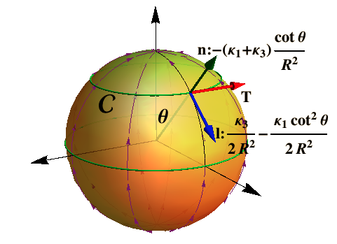
Figure 4: Nematic texture with $\Theta=\pi/2$, and the induced local forces $F_{l}$ and $F_{n}$; with this texture, the equilibrium equation is given by Eq. (45).

For this nematic texture, the intrinsic torque on parallels is given by

$${\bf m}^{a}l_{a}=-\left[\frac{\kappa_{3}}{R}+\kappa\left(\frac{2}{R}-K_{0}\right)\right]\boldsymbol{\phi}.$$ (52)

Therefore, the couple due to the nematic texture adds to the bending one, and counteracts to the effect of the spontaneous curvature. On the meridians, the intrinsic nematic torque vanishes.

VI.2 Nematic texture with $\Theta=0$

This texture represents an orientation along spherical parallels; here, we identify $\boldsymbol{\eta}={\bf T}$ and $\boldsymbol{\eta}_{\perp}={\bf l}$ (see Fig. 5). In this case, the divergence of the nematic field vanishes, thus the nematic texture does not induce splay forces; let’s notice that $\eta^{a}l_{a}=0$. Consequently, the non-trivial terms are $\eta^{a}\nabla_{a}\eta^{\theta}=-\cot\theta/R^{2}$, and the normal curvature at the parallel, $K_{\eta}=1/R$, which determines the longitudinal components of the bending force, $F_{l}^{B}$ in Eq. (23). As a consequence, the total force points along the conormal ${\bf l}$. Once the elastic force is considered, we found

$$F_{l}=-\Sigma+\frac{\kappa K_{0}}{R}-\frac{\kappa_{3}}{2R^{2}}(1+\cot^{2}\theta).$$ (53)

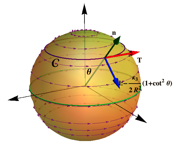
Figure 5: The nematic texture $\Theta=0$, on the sphere. The only non trivial local force points along the conormal $\bf l$.

The bend force on the entire loop (except for them close to the poles) is a constant and points upward as

$${\bf F}_{B}=\frac{\pi\kappa_{3}}{R}{\bf k}.$$ (54)

In this case, the equilibrium equation can be expressed as

$$\frac{PR}{2}=\Sigma-\frac{\kappa K_{0}}{R}+\frac{\kappa_{3}}{2R^{2}}\left(1+\cot^{2}\theta\right),$$ (55)

which only contains elasticity and nematic bending terms playing against each other. Splay and twist terms are missing in this case as they do not contribute to distort the parallels.

Because on parallel loops, the condition $\boldsymbol{\eta}\cdot{\bf l}=0$ holds, here, the intrinsic nematic torque vanishes and the total intrinsic torque is given by

$${\bf m}^{a}l_{a}=-\kappa\left(\frac{2}{R}-K_{0}\right)\boldsymbol{\phi}.$$ (56)

On meridians, we can find instead

$${\bf m}^{a}l_{a}=-\left[\frac{\kappa_{3}}{R}+\kappa\left(\frac{2}{R}-K_{0}\right)\right]\boldsymbol{\theta}.$$ (57)

Therefore, the nematic couple adds up to the bending one and counteracts the effect of the spontaneous curvature.

VII Stress on cylindrical surfaces

A cylindrical surface of radio $R$ and length $L$ can be parametrized as

$${\bf X}(\phi,z)=(R\cos\phi,R\sin\phi,z),$$ (58)

where the azimuthal angle varies in the full domain $0\leq\phi<2\pi$, and $z\in[-L/2,L/2]$. The tangent vectors are expressed as ${\bf e}_{\phi}=R\boldsymbol{\phi}$ and ${\bf e}_{z}={\bf k}$, whereas the unit normal is ${\bf n}=(\cos\phi,\sin\phi,0)$. On the surface $ds^{2}=dz^{2}+R^{2}d\phi^{2}$, gets the infinitesimal distance whereas $K_{\phi\phi}=R$ and $K_{zz}=0,K_{z\phi}=0$ are the components of the extrinsic curvature. In this geometry, if the nematic texture is directionally aligned on meridians, the Frank energy exactly vanishes. Consequently, with the exception of the pure elastic force, no additional force have to be overcome to suction a tube in a cylindrical micropipette. Unlike, if the nematic director aligns with parallels, the components are $\eta^{\phi}=1/R$ and $\eta^{z}=0$ (see Fig. 6), and thus the bend energy density becomes $\kappa_{3}/2R^{2}$. In this case the membrane energy reads in terms of the tube dimensions as

$$H=\sigma A+\frac{\kappa A}{2}\left(\frac{2\pi L}{A}-K_{0}\right)^{2}+\frac{\kappa_{3}}{2}\frac{4\pi^{2}L^{2}}{A},$$ (59)

where $A=2\pi RL$ is the cylinder area. If the tube length is fixed at $L$, then the condition $\partial_{A}H=0$ determines the equilibrium radius at $R_{\rm eq}=\sqrt{(\kappa+\kappa_{3})/2\Sigma}$, where the energy reaches a minimum and we have introduced $\Sigma=\sigma+\kappa K_{0}^{2}/2$. In the absence of bending nematics, this formula reduces to the classical result for the equilibrium radius of a lipid tube, $R_{\rm eq}=\sqrt{\kappa/\Sigma}$.
A more general result, can be also obtained by cancelling out the stress around the symmetry axis. For a general texture as in Fig. 7, let’s consider

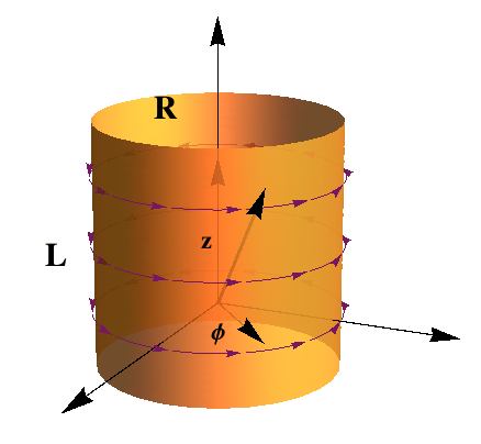
Figure 6: The nematic texture $\eta^{\phi}=1/R$ and $\eta^{z}=0$ on the cylinder, if $L$ is fixed then $R=\sqrt{(\kappa+\kappa_{3})/2\Sigma}$.

$$\boldsymbol{\eta}=\cos\alpha\,\boldsymbol{\phi}+\sin\alpha{\bf k},$$ (60)

to be the nematic director oriented at an angle $\alpha$ with respect to the unit azimuthal vector $\boldsymbol{\phi}$ ( see Fig. 7). The components are then $\eta^{\phi}=\cos\alpha/R$ and $\eta^{z}=\sin\alpha$. We also see that $\boldsymbol{\eta}_{\perp}=\sin\alpha\,\boldsymbol{\phi}-\cos\alpha\,{\bf k}$. Additionally, since $\eta_{a}l^{a}=-\sin\alpha$, $\eta^{a}_{\perp}l_{a}=\cos\alpha$, $\eta^{b}T_{b}=\cos\alpha$, $K_{ab}\eta^{a}l^{b}=0$, $K_{ab}\eta^{a}T^{b}=\cos\alpha/R$, one obtains

$$\nabla_{a}\eta^{a} = 0,$$

$$K_{\eta} = \frac{\cos^{2}\alpha}{R},$$

$$K_{\tau} = \frac{\sin\alpha\cos\alpha}{R}.$$ (61)

Because the divergence of the texture is exactly null in this case, the splay force vanishes as well. Therefore, the components of the local force on the loop can be written as

$$F_{T} = \frac{\kappa_{2}}{R^{2}}\sin\alpha\cos^{3}\alpha,$$

$$F_{l} = -\frac{\kappa_{2}}{2R^{2}}\sin^{2}\alpha\cos^{2}\alpha-\frac{\kappa_{3}}{2R^{2}}\cos^{4}\alpha,$$

$$F_{n} = 0.$$ (62)

In a circular parallel loop, the normal force is found identically zero, as expected for a tube at mechanical equilibrium. However, the two in-plane components adopt non-trivial dependences on the orientation $\alpha$ of the texture. Whereas the longitudinal component is affected by twisting and bending nematic terms, the tangential component that maintains the circulation around the tube axis is exclusively determined by twisting. The total force on the entire loop is given by

$${\bf F}=2\pi R\,(F_{l}\,{\bf l}+F_{T}{\bf T}).$$ (63)

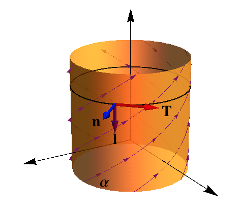
Figure 7: The nematic texture (60) on the cylinder, $\alpha$ being the angle of the nematic director with the horizontal. The only non trivial local force points along the conormal ${\bf l}$ in eq.(64). On this loop, $T^{\phi}=1/R$, $T^{z}=0$, $l^{\phi}=0$, $l^{z}=-1$, are the components of the Darboux basis.

In the particular case of the parallel texture, $\alpha=0$ (see Fig. 6) only the bending force determines the longitudinal component $F_{l}=-\kappa_{3}/2R^{2}$; in the opposite case, $\alpha=\pi/2$, then $F_{l}=0$. With the intermediate texture, $\alpha=\pi/4$, we found $F_{T}=\kappa_{2}/4R^{2}$ and $F_{l}=-\frac{1}{8R^{2}}(\kappa_{2}+\kappa_{3}).$
We further consider the case of meridian directions along the cylinder axis, where ${\bf T}={\bf k}$, thus $T^{z}=1$ and $T^{\phi}=0$; here ${\bf l}={\bf e}_{\phi}/R$ and $l^{\phi}=1/R$, thus $K_{l}=1/R$ and $K_{T}=0$. Therefore, $\eta^{a}l_{a}=\cos\alpha$, $\eta^{b}T_{b}=\sin\alpha$, $K_{ab}\eta^{a}l^{b}=\cos\alpha$, $K_{ab}\eta^{a}T^{b}=0$. Consequently, the components of the force are found as

$$F_{T} = 0,$$

$$F_{l} = -\frac{\kappa_{2}}{2R^{2}}\sin^{2}\alpha\cos^{2}\alpha+\frac{\kappa_{3}}{2R^{2}}\cos^{4}\alpha,$$

$$F_{n} = 0,$$ (64)

i.e. only the longitudinal component is non zero in this case. In fact, we can adjust the radius of the cylinder, such that the stress on any meridian vanishes. This experiment could consist to fix the nematic texture at rotational orientation ($\alpha=0$), then $R_{\rm eq}=\sqrt{(\kappa+\kappa_{3})/2\Sigma}$, independently of the splay and twisting rigidities. In the uniaxial orientation ($\alpha=\pi/2$), the equilibrium radius reduces becomes exclusively determined by membrane elasticity, i.e. $R_{\rm eq}=\sqrt{\kappa/2\sigma}$, which determines a much smaller tensions than necessary to realize the rotational texture. In the most general case, we found tubes with equilibrium radius

$$R_{\rm eq}=\sqrt{(\kappa+\kappa_{3}\cos^{4}\alpha-\kappa_{2}\sin^{2}\alpha\cos^{2}\alpha)/2\Sigma}.$$ (65)

On parallels, the torque can be written as

$${\bf m}^{a}l_{a} = \Big{[}\frac{\sin\alpha\cos\alpha}{R}(\kappa_{2}\cos^{2}\alpha-\kappa_{3}\sin^{2}\alpha)$$ (66)

$$- \kappa\left(\frac{1}{R}-K_{0}\right)\Big{]}\boldsymbol{\phi}$$

$$- \frac{\cos^{2}\alpha}{R}(\kappa_{2}\cos^{2}\alpha-\kappa_{3}\sin^{2}\alpha){\bf k}.$$

The nematic texture with $\alpha=\pi/2$, does not induce nematic intrinsic torque, as expected. If $\alpha=0$, we find ${\bf m}^{a}l_{a}=-\kappa(1/R-K_{0})\boldsymbol{\phi}-\kappa_{2}/R\,{\bf k}$, and the twist does not play in the couple. Nevertheless, any deviation of the circular texture, induces a contribution of the twist; if $\alpha=\pi/4$ we have

$${\bf m}^{a}l_{a}=\frac{1}{4R}(\kappa_{2}-\kappa_{3}-4\kappa)\boldsymbol{\phi}-\frac{1}{4R}(\kappa_{2}-\kappa_{3}){\bf k}.$$ (67)

Importantly, the local torque induced by the twist counteracts the one induced by the bending mode of the director field.

VIII discussion

We have obtained analytical expressions for the stress tensor and the torque of an elastic membrane decorated with a nematic texture constrained to lie tangent to the membrane. The nematic texture is modeled by the Frank energy, which takes into account splay, twist and bend orientations of the nematic director. A pure geometric standpoint is adopted to get the distribution of internal forces due to local coupling between the nematic field and membrane curvature. Specifically, the geometric characteristics of the nematic field (tangential $\boldsymbol{\eta}\cdot{\bf n}=0$, and normalized $\boldsymbol{\eta}\cdot\boldsymbol{\eta}=1$), together with the surface metric and its curvature, are connected to the embedding function that defines the surface by introducing auxiliary variables that impose the appropriate constraints. The method of auxiliary variables, previously developed by Guven to impose geometric congruence for generalized quadratic constraints auxiliary ; jemal-book , has been here re-adapted to identify the components of the surface stress tensor after the different terms of the nematic field. The structure of the membrane stress tensor exhibits a non-trivial interplay between nematic structure and geometry, showing the relevance of the extrinsic effects, particularly of the coupling between nematic director and extrinsic membrane curvature. For instance, whereas the surface stress induced by nematic splaying exhibits a tangential component with only intrinsic coupling, the normal component is chiefly driven by extrinsic curvature.

In general, the internal forces appeared in the membrane become very intense at regions where the divergence of the nematic director increases, which correspond to membrane locations where topological defects are placed in. Expectedly, textures with zero divergence do not induce these forces, maintaining unchanged the orientation of the nematics over the whole surface. The bending stress induced by the nematic director really dominates in curved surfaces by through of tangential components produced by extrinsic couplings; in fact, if the nematic director is aligned on geodesics, only extrinsic effects do contribute. As regards twisting stresses, they exclusively arise from extrinsic couplings. Globally, our results constitute a first achievement on the mechanics of nematic membranes, an intriguing problem early captivating attention of several communities (see reviews in refs. kamien ; giomi ), but still remained unresolved because an analytics extremely complex. Although the approach here adopted is not mechanical in nature, but merely geometric indeed, the method of auxiliary variables with surface-based constraints has delivered a complete description of the nematic membrane stresses.
Specifically, the forces on circular loops have been calculated for different textures in spherical and a cylindrical settings chen-kamien . For the spherical case, two nematic textures of interest have been analyzed; the first is the case of meridian orientation with finite divergence and a defect at each pole, and the second corresponds to parallel orientation with zero divergence. In both cases, we have obtained the corresponding equilibrium force equation including the elastic bending and the Laplace pressure at mechanical trade-off with the nematic forces. For the meridian texture, both, splay and bending modes play a non-trivial role. However, for the parallel texture, only the bending constant intervenes in the equilibrium equation. The results here obtained are equivalent to the theory of nematic films in Delaunay surfaces, which has been previously developed by Chen and Kamien chen-kamien . Similarly to our results for the ”parallel” nematic orientation (Eqs. (53)-(57) for the sphere and Eqs. (62)-(67) for the cylinder), these authors predicted nematic configurations that are automatically splay-free if lying parallel to the lines of latitude of a surface of revolution chen-kamien . A phase-diagram of stable shapes and topologies was mapped in that theoretical work, a breakthrough that could be generalized using our theory. From the equilibrium equation in Eq. (45), we can estimate a persistence length scale for nematic effects; specifically, $l_{\Sigma}=2\Sigma R^{2}/\kappa_{1}$ in the regime of high membrane tension at high nematic alignment, and $l_{\kappa}\approx 2\kappa/\kappa_{3}$ if bending rigidity governs. Taking typical values $\kappa_{1}\approx 10^{-11}\,N$ and $\kappa_{3}\approx 10^{-9}N$, for nanometric shells ($R\approx 10\,nm$), we estimate $l_{\kappa}\approx 10\,nm$ in the case of a relatively rigid membrane ($\kappa\approx 20k_{B}T$), and $l_{\Sigma}\approx\,100\,nm$ in the tensioned case membrane ($\Sigma\approx 10^{-2}N/m$). These predicted scales oversize the systemic dimensions, thus confirming the dominance of the molecular director to determine the configuration of nanometric-sized nematic shells $(l\gg R)$. Our estimates as agree well with previous conclusion by Chen and Kamien for thin film with a revolutionary symmetry, where anisotropic nematic effects were predicted to dominate the membrane shape chen-kamien . At very high tension, these ordering effects can eventually oversize the molecular dimensions up to the macroscopic scale; in the tensioned membrane of a biological cell, for instance ($R\approx 10\,\mu m;\Sigma\gg 10^{-2}N/m$). Otherwise said, the characteristic length becomes larger than the characteristic cell size $(l_{\Sigma}\gg R)$, which is due to the strong persistence of the molecular alignment supported by a high lateral tension. On the cylinder, a texture such that its nematic director follows helical trajectories has been analyzed and the forces on parallels and meridians have been obtained. Interestingly, there are no induced forces when the nematic director is aligned along the cylinder axis. If one considers the director aligned on parallels, we find that the nematic tension, has a finite magnitude of $\kappa_{3}/2R$, which contributes to stiff the tube beyond its mere flexural elasticity. In the case of a nanometric tube with a nematic membrane ($R\approx 10\,nm$), for example a cylindrical vesicle made of oriented polymers, or mitochondrial cristae in the cell biology setting, the membrane tension due to anisotropic ordering should take a value of the order of $\kappa_{3}/2R\approx 0.1\,N/m$, at least one order of magnitude higher than the typical tensions of isotropic membranes. Regarding the torque within these nematic membranes, we have found that no intrinsic torque is induced, in general, by splaying the nematic director. This is because the splay energy is purely intrinsic to the membrane and the nematic director is deformed perpendicular to the membrane. As a consequence, splay contributes only to the external torque. Particularly for the sphere, there are no twist contributions too, so only the bending plays a role in the torque, unlike the cylinder geometry where twist and bend play both a relevant role.

Our geometric theory of the mechanics of nematic membranes builds upon the barest case of fluid isotropic membranes, which is harnessed by the Canham-Helfrich theory stress ; deserno ; fournier ; napoli2010 . The early antecedent to a mechanical theory of fluid membranes with in-plane order was focussed on texture topology mac , but not in membrane curvature, as we elaborate here. The ad hoc introduction of curvature terms in the Frank’s energy of nematic shells has been also considered in studies of structure vinel , stability sonnet and geometry-induced distortions in molecular director vergori . However, despite the capacity of those approaches in describing the frustrations in nematic ordering elicited by membrane geometry, a closed theory of the ordering-curvature coupling completely congruent with geometry is still lacking. The previous work by Chen and Kamien already pointed out the chief role of the nematic bending to elicit spontaneous curvature anisotropy leading to shape instability chen-kamien . That study on surfaces of revolution predicted surface buckling, even topological transitions (sphere-torus), at well defined material regimes of tension-to-bending nematic rigidity chen-kamien . Unstable scenarios have been also described in previous works as a consequence of either electrically-induced molecular tilting New5 or defect interactions kardar . Here, we have considered the Frank’s energy in a complete geometry-structure coupling schema in which the nematic field is affinelly embedded in the curvature-elasticity field. Our unprecedented achievement represents a major novelty as provides a closed framework to predict the equilibrium distribution of membrane stresses in generalized geometry. This definitively opens a gate to the generalized mechanics of nematic membranes, including the dynamics of shape transformations and stability analyses.
In the biological setting, the theoretical framework here developed could contribute a better understanding of the mechanical remodeling effected by ordered structures (nematic-like) on flexible membranes. As a relevant example, our theory could be exploited to model local forces in cellular membranes. During early stages of cell division, particularly along the cytokinetics processes, specifically aligned actomyosin filaments present in the division forrow are known to induce constriction forces at cell equator. This dynamic process arises from a mechanical interplay settled in the membrane between cytokinetic ordering forces and geometric couplings, which finally leads to divisional cell remodeling. Our FCH-theory of nematic-membranes could pave the unexplored way to link dynamical ordering inside the cell cortex and cytokinetic forces.

IX CONCLUSIONS

This work addresses a geometric approach to the mechanics of nematic membranes as described by the Frank-Canham-Helfrich (FCH) energy. Using the method of auxiliary variables, we have given account for the surface-based constraints that define the geometric characteristics of the coupling connections between membrane curvatures and nematic director. The FCH theory here developed provides an analytic framework to predict the distribution of nematic membrane forces, both tensional stresses and torques, which arise from intrinsic and extrinsic curvature couplings with the molecular director. The nature and the strength of the different couplings have been neatly identified, and their impact in the geometric distortion of the nematic ordering evaluated in simple geometrical settings (sphere and cylinder). Although the current theory is essentially geometric, the results approached open a new gate towards the still unavailable mechanical theory of nematic membranes with possible biological applications. Further work on the theoretical implications of the geometric approach to the FCH field, and its possible extension to a more sophisticated mechanical theory, is ongoing.

Appendix A Stress tensor

In order to obtain the stress ${\bf f}^{a}$, we adapt the method of auxiliary variables auxiliary ; jemal-book , to implement the geometric constraints related with the several objects $\Sigma$ describing the surface structure; these are: ${\bf e}_{a}\cdot{\bf n}=0$, $g_{ab}={\bf e}_{a}\cdot{\bf e}_{b}$, ${\bf n}\cdot{\bf n}=1$, ${\bf e}_{a}=\partial_{a}{\bf X}$, and $K_{ab}={\bf e}_{a}\cdot\nabla_{b}{\bf n}$. The functional to be minimized is written by introducing the corresponding Lagrange multipliers as

$$H=H_{\rm Frank}+\int dA\,\,[{\bf f}^{a}\cdot({\bf e}_{a}-\partial_{a}{\bf X})+\frac{\Lambda}{2}({\bf n}\cdot{\bf n}-1)$$ (68)

$$+\Lambda^{a}({\bf n}\cdot{\bf e}_{a})+\Lambda^{ab}(K_{ab}-{\bf e}_{a}\cdot\partial_{a}{\bf n})$$

$$+ \frac{\lambda^{ab}}{2}(g_{ab}-{\bf e}_{a}\cdot{\bf e}_{b})].$$

In order to applied the auxiliary method, the Frank’s energy must be written explicitly in terms of the geometric variables as

$$({\nabla}\cdot\boldsymbol{\eta}) = g^{ab}({\bf e}_{a}\cdot\nabla_{b}\boldsymbol{\eta}),$$

$$\boldsymbol{\eta}\cdot({\nabla}\times\boldsymbol{\eta}) = g^{ab}\boldsymbol{\eta}\cdot({\bf e}_{a}\times\nabla_{b}\boldsymbol{\eta}),$$

$$(\boldsymbol{\eta}\cdot{\nabla})\boldsymbol{\eta} = g^{ab}\boldsymbol{\eta}\cdot{\bf e}_{a}\nabla_{b}\boldsymbol{\eta}.$$ (69)

If one is interested in closed vesicles then a constraint that fixes the volume enclosed will be needed jiang . The variation with respect to the embedding function ${\bf X}$ gives

$$\delta H=\int dA\nabla_{a}{\bf f}^{a}\cdot\delta{\bf X}-\int ds\,l_{a}{\bf f}^{a}\cdot\delta{\bf X},$$ (70)

so that Euler-Lagrange equation implies the conservation law $\nabla_{a}{\bf f}^{a}=0$. On the one hand, variation of the functional $H$ respect the the tangent vectors gives

$$\delta H = \int dA(A^{ac}{\bf e}_{c}-B^{a}{\bf n})\cdot\delta{\bf e}_{a}$$ (71)

$$+ \int dA\,[{\bf f}^{a}+\Lambda^{a}{\bf n}-\Lambda^{ab}\partial_{a}{\bf n}-\lambda^{ab}{\bf e}_{b}]\cdot\delta{\bf e}_{a},$$

with coefficients

$$A^{ac} = \kappa_{1}\nabla_{d}\eta^{d}\nabla^{a}\eta^{c}+\kappa_{2}K_{\tau}K^{a}{}_{b}\eta^{b}\eta^{c}_{\perp}$$

$$+ \kappa_{3}(\eta^{d}\nabla_{d}\eta^{b}\nabla^{a}\eta_{b}+K_{\eta}\eta^{b}K_{b}{}^{a})\eta^{c}$$

$$B^{a} = \kappa_{1}\nabla_{d}\eta^{d}K^{a}{}_{c}\eta^{c}-\kappa_{2}K_{\tau}\eta_{\perp c}\nabla^{a}\eta^{c}$$ (72)

and $K_{\eta}=K_{ab}\eta^{a}\eta^{b}$, $K_{\tau}=K_{ab}\eta^{a}_{\perp}\eta^{b}$. Therefore, we find the stress tensor as

$${\bf f}^{a}=(\lambda^{ac}+\Lambda^{ab}K_{b}{}^{c}-A^{ac}){\bf e}_{c}-(\Lambda^{a}-B^{a}){\bf n}.$$ (73)

On the other hand, variation of the functional $H$ with respect to the normal ${\bf n}$ gives

$$\delta H=\int dA[\lambda\boldsymbol{\eta}+\Lambda{\bf n}+\Lambda^{a}{\bf e}_{a}+\nabla_{b}(\Lambda^{ab}{\bf e}_{b}))]\cdot\delta{\bf n},$$ (74)

and because linear independence we have

$$\Lambda-\Lambda^{ab}K_{ab} = 0,$$

$$\lambda\eta^{a}+\Lambda^{a}+\nabla_{b}\Lambda^{ab} = 0.$$ (75)

Here, the Lagrange multiplier $\Lambda^{ab}$ vanishes because the extrinsic curvature components $K_{ab}$ do not appear explicitly into the energy $H_{\rm Frank}$. The fact that the metric $g_{ab}$ appears into $H_{\rm Frank}$, determines the Lagrange multiplier $\lambda^{ab}=T^{ab}$, where $T^{ab}$ is the tensor defined by the variation

$$\delta H_{\rm Frank}=-\frac{1}{2}\int dA\,T^{ab}\,\delta g_{ab}.$$ (76)

In the calculation of this variation, we cast $\delta g^{ab}=-g^{ac}g^{bd}\delta g_{cd}$. After some algebra, we find

$$T^{ab}_{S} = \kappa_{1}[({\bf e}^{c}\cdot\nabla_{c}\boldsymbol{\eta})({\bf e}^{a}\cdot\nabla^{b}{\bf\boldsymbol{\eta}}+{\bf e}^{b}\cdot\nabla^{a}{\bf\boldsymbol{\eta}})-\frac{g^{ab}}{2}({\bf e}^{c}\cdot\nabla_{c}\boldsymbol{\eta})^{2}],$$

$$= \kappa_{1}(\nabla_{c}\eta^{c})\Big{[}(\nabla^{a}\eta^{b}+\nabla^{b}\eta^{a})-\frac{g^{ab}}{2}(\nabla_{d}\eta^{d})\Big{]},$$

$$T^{ab}_{W} = \kappa_{2}[K_{\tau}\boldsymbol{\eta}\cdot({\bf e}^{a}\times\nabla^{b}\boldsymbol{\eta}+{\bf e}^{b}\times\nabla^{a}\boldsymbol{\eta})$$

$$-\frac{g^{ab}}{2}(g^{cd}\boldsymbol{\eta}\cdot({\bf e}_{c}\times\nabla_{d}\boldsymbol{\eta}))^{2}],$$

$$= \kappa_{2}[K_{\tau}(K_{cb}\eta^{c}\eta_{\perp a}+K_{ca}\eta^{c}\eta_{\perp b})-\frac{g^{ab}}{2}K_{\tau}^{2}],$$

$$T^{ab}_{B} = \kappa_{3}\,\eta^{d}\nabla_{d}\boldsymbol{\eta}\cdot[\eta^{a}\nabla^{b}\boldsymbol{\eta}+\eta^{b}\nabla^{a}\boldsymbol{\eta}-\frac{g^{ab}}{2}\eta^{c}\nabla_{c}\boldsymbol{\eta}]$$ (77)

$$= \kappa_{3}\,[K_{\eta}\eta^{c}(\eta^{a}K^{b}{}_{c}+\eta^{b}K^{a}{}_{c})$$

$$+ \eta^{d}\nabla_{d}\eta^{c}(\eta^{a}\nabla^{b}\eta_{c}+\eta^{b}\nabla^{a}\eta_{c})$$

$$- \frac{g^{ab}}{2}(\eta^{d}\eta^{e}\nabla_{d}\eta^{c}\nabla_{e}\eta_{c}+K_{\eta}^{2})].$$

The stress is then written as

$${\bf f}^{a}=(T^{ac}-A^{ac}){\bf e}_{c}-(\Lambda^{a}-B^{a}){\bf n},$$ (78)

where the multiplier $\Lambda^{a}$ will be determined once the multiplier $\lambda$ does. To find $\Lambda^{a}$ we calculate the variation of the energy Eq. (68) under deformations of the field itself; up to a boundary terms, we have

$$\delta H=\int dA(C^{a}{\bf e}_{a}+D{\bf n})\cdot\delta\boldsymbol{\eta}+\int dA(\beta\boldsymbol{\eta}+\lambda{\bf n})\cdot\delta\boldsymbol{\eta}$$ (79)

where

$$C^{a} = -{\kappa}_{1}g^{ab}\nabla_{b}\nabla_{c}\eta^{c}+{\kappa}_{2}K_{\tau}(2K_{bc}\eta^{b}\varepsilon^{ca}+K\eta^{a}_{\perp})$$

$$+{\kappa}_{3}[\eta^{b}\nabla_{b}\eta_{d}(\nabla^{a}\eta^{d})-\nabla_{b}\eta^{b}(\eta^{c}\nabla_{c}\eta^{a})-\eta^{b}\nabla_{b}\eta^{c}(\nabla_{c}\eta^{a})$$

$$-\eta^{b}\eta^{c}\nabla_{b}\nabla_{c}\eta^{a}+2K_{\eta}K^{a}{}_{b}\eta^{b}]$$

$$D = {\kappa}_{1}\nabla_{a}\eta^{a}K+{\kappa}_{2}(2K_{\tau}\nabla_{a}\eta^{a}_{\perp}+\eta^{a}_{\perp}\nabla_{a}K_{\tau})$$ (80)

$$+\kappa_{3}[\nabla_{b}\eta^{b}K_{\eta}+\eta^{b}\nabla_{b}\eta^{a}K_{ad}\eta^{d}$$

$$+\eta^{b}\eta^{c}(\nabla_{c}\eta^{d}K_{bd}+\nabla_{b}K_{cd}\eta^{d}+K_{cd}\nabla_{b}\eta^{d})]$$

with the missing Lagrange multipliers being $\lambda=-D$ and $\beta=-C^{a}\eta_{a}$, so that $\Lambda^{a}=D\eta^{a}$. Then, we can write

$${\bf f}^{a}=(T^{ac}-A^{ac}){\bf e}_{c}-(D\eta^{a}-B^{a}){\bf n},$$ (81)

where the values of $T^{ab}$, $A^{ab}$ and $B^{a}$ should be substituted by their corresponding expressions above expanded. Thus, we find that the splay stress tensor becomes proportional to the divergence of the director field. It can be written as

$${\bf f}^{a}_{S} = \kappa_{1}\nabla_{d}\eta^{d}\left(\nabla^{c}\eta^{a}-\frac{g^{ac}}{2}\nabla_{d}\eta^{d}\right){\bf e}_{c}$$ (82)

$$- \kappa_{1}\nabla_{c}\eta^{c}(K\eta^{a}-K^{a}{}_{c}\eta^{c}){\bf n},$$

where the tangential components have intrinsic information of the surface through the metric $g_{ab}$ and the covariant derivatives of $\eta^{a}$. The normal projection has, instead, coupling with extrinsic curvature. The splay force per unit length can then be written as

$${\bf f}^{a}_{S}l_{a}=F_{T}{\bf T}+F_{l}{\bf l}+F_{n}{\bf n},$$ (83)

where the projections are given by

$$F_{T} = \kappa_{1}\nabla_{d}\eta^{d}T^{c}l^{a}\nabla_{c}\eta_{a},$$

$$F_{l} = \kappa_{1}\nabla_{d}\eta^{d}\left(l^{a}l^{c}\nabla_{c}\eta_{a}-\frac{1}{2}\nabla_{b}\eta^{b}\right),$$

$$F_{n} = -\kappa_{1}\nabla_{d}\eta^{d}(K\eta_{a}l^{a}-K_{ab}l^{a}\eta^{b}).$$ (84)

As expected, the extrinsic coupling appears only in the normal projection. The twist stress tensor is identified as:

$${\bf f}_{W}^{a} = \kappa_{2}K_{\tau}(K^{cb}\eta_{c}\eta_{\perp}^{a}-\frac{g^{ab}}{2}K_{\tau}){\bf e}_{b}$$ (85)

$$- \kappa_{2}[(2K_{\tau}\nabla_{c}\eta^{c}_{\perp}+\eta^{c}_{\perp}\nabla_{c}K_{\tau})\eta^{a}$$

$$+ K_{\tau}\eta_{\perp c}\nabla^{a}\eta^{c}]{\bf n},$$

where all the terms have coupling with extrinsic curvature. In this case, we have

$$F_{T} = \kappa_{2}K_{\tau}K_{cb}\eta^{c}T^{b}\eta_{\perp}^{a}l_{a},$$

$$F_{l} = \kappa_{2}K_{\tau}\left(K_{cb}\eta^{c}l^{b}\eta_{\perp}^{a}l_{a}-\frac{K_{\tau}}{2}\right),$$

$$F_{n} = -\kappa_{2}[(2K_{\tau}\nabla_{c}\eta^{c}_{\perp}+\eta^{c}_{\perp}\nabla_{c}K_{\tau})\eta^{a}l_{a}$$ (86)

$$+ K_{\tau}\eta_{\perp c}l^{a}\nabla_{a}\eta^{c}].$$

Finally, the bend stress tensor can be obtained as

$${\bf f}_{B}^{a} = \kappa_{3}\Big{[}K_{\eta}\eta^{c}\eta^{a}K^{b}{}_{c}+\eta^{a}\eta^{d}\nabla_{d}\eta^{c}\nabla^{b}\eta_{c}$$ (87)

$$- \frac{g^{ab}}{2}(\eta^{d}\eta^{e}\nabla_{d}\eta^{c}\nabla_{e}\eta_{c}+K_{\eta}^{2})\Big{]}{\bf e}_{b}$$

$$- \kappa_{3}\Big{[}\nabla_{b}\eta^{b}K_{\eta}+3\eta^{b}\nabla_{b}\eta^{c}K_{cd}\eta^{d}$$

$$+ \eta^{b}\eta^{c}\eta^{d}\nabla_{b}K_{cd}\Big{]}\eta^{a}{\bf n}.$$

Therefore, we can obtain the projections as

$$F_{T} = \kappa_{3}[K_{\eta}K_{bc}T^{b}\eta^{c}+\eta^{d}\nabla_{d}\eta^{c}T^{b}\nabla_{b}\eta_{c}]\eta^{a}l_{a}$$

$$F_{l} = \kappa_{3}[K_{\eta}K_{bc}l^{b}\eta^{c}+\eta^{d}\nabla_{d}\eta^{c}l^{b}\nabla_{b}\eta_{c}]\eta^{a}l_{a}$$

$$- \frac{\kappa_{3}}{2}\left(\eta^{d}\eta^{e}\nabla_{d}\eta^{c}\nabla_{e}\eta_{c}+K_{\eta}^{2}\right)$$

$$F_{n} = -\kappa_{3}\Big{[}\nabla_{b}\eta^{b}K_{\eta}+3\eta^{b}\nabla_{b}\eta^{c}K_{cd}\eta^{d}$$ (88)

$$+ \eta^{b}\eta^{c}\eta^{d}\nabla_{b}K_{cd}\Big{]}\eta^{a}l_{a}$$

References

• (1) W. Helfrich and J. Prost, Intrinsic bending force in anisotropic membranes made of chiral molecules, Phys. Rev. A 38 (6) 3065 (1988).
• (2) R.D. Kamien, The geometry of soft materials: a primer, Reviews of Modern Physics. Vol. 74, 953 (2002).
• (3) M.J. Bowick and L. Giomi, Two-dimensional matter: order, curvature and defects, Advances in Physics 58 (5), 449 (2009).
• (4) J.A. Santiago, Stresses in curved nematic membranes, Phys. Rev. E 97, 052706 (2018).
• (5) P. B. Canham, The minimum energy of bending as a possible explanation of the biconcave shape of the human red blood cell, Journal of theoretical Biology 26, (1969).
• (6) W. Helfrich, Elastic properties of lipid bilayers: theory and possible experiments, Z. Naturforsch 28 c (1973).
• (7) Ou-Yang Zhong-can, Elastic theory of biomembranes, Thin Solid Films 393 19 (2001).
• (8) Ou-Yang Zhong-can and W. Helfrich, Instability and Deformation of a Spherical Vesicle by Pressure, Phys. Rev. Lett. 59, 2486 (1987); Erratum Phys. Rev. Lett. 60, 1209 (1988).
• (9) Ou-Yang Zhong-can and W. Helfrich, Bending energy of vesicle membranes: General expressions for the first, second, and third variation of the shape energy and applications to spheres and cylinders, Phys. Rev. A 39, 5280 (1989).
• (10) P. G. de Gennes, The Physics of Liquid Crystals, (Oxford Unversity Press, Oxford, 1993).
• (11) G. Napoli and L. Vergori, Extrinsic curvature effects on nematic shells, Phys. Rev. Lett. 108, 207803 (2012).
• (12) B. L. Mbanga, G.M. Grason and C.D. Santangelo, Frustrated Order on Extrinsic Geometries, Phys. Rev. Lett. 108, 017801 (2012).
• (13) J.R. Frank and M. Kardar, Defects in nematic membranes can buckle into pseudospheres, Phys. Rev. E 77, 041705 (2008).
• (14) T.S. Nguyen, J. Geng, R.L.B Selinger and J.V. Selinger, Nematic order on a deformable vesicle: theory and simulation, Soft Matter 9, 8314 (2013).
• (15) H. Aharoni and E. Sharon, Geometry of Thin Nematic Elastomer Sheets, Phys. Rev. Lett. 113, 257801 (2014).
• (16) Y. Yu, M. Nakano and T. Ikeda. Directed bending of a polymer film by light, Nature 425, 145 (2003).
• (17) G. N. Mol, K. D. Harris, C. W. M. Bastiaansen, and D. J. Broer. Thermo-Mechanical Responses of Liquid-Crystal Networks with a Splayed Molecular Organization, Adv. Funct. Mater. 15, 1155 (2005).
• (18) H. Aharoni, Y. Xia, X. Zhang, R.D. Kamien and S. Yang. Universal inverse design of surfaces with thin nematic elastomer sheets, Proc. Nat. Acad. Sci. 115, 7206 (2018).
• (19) B.G. Chen and R.D. Kamien, Nematic films and radially anisotropic Delaunauy surfaces, Eur. Phys. J. E 28, 315 (2009.)
• (20) R. Capovilla and J. Guven, Stresses in lipid membranes, J. of Physics A: Math. Gen. 35, 6233 (2002).
• (21) R. Capovilla, J. Guven and J.A. Santiago, Deformation of the geometry of lipid vesicles, J. Phys. A: Math. Gen. 36, 6281 (2003).
• (22) J.B. Fournier, On the stress and torque tensors in fluid membranes, Soft Matter 3, 883 (2007).
• (23) A. M. Turner, V. Vitelli, and D. R. Nelson, Vortices on curved surfaces, Rev. Mod. Phys 82, 1301 (2010).
• (24) H. Shin, M.J. Bowick and X. Xing, Topological defects in spherical nematics Phys. Rev. Lett. 101, 037802 (2008).
• (25) T. Lopez-Leon and A. Fernandez-Nieves, Drops and shells of liquid crystal, Colloid Polym. Sci. 289, 345 (2011).
• (26) M. Bates in Fluids, Colloids and Soft Materials: An Introduction to Soft Matter Physic, Edited by Alberto Fernandez Nieves and Antonio Manuel Puertas, (John Wiley and Sons, Inc. 2016).
• (27) G. Napoli and L. Vergori, Equilibrium of nematic vesicles, J. Phys. A: Math. Theor. 43, 445207 (2010).
• (28) G. Napoli and L. Vergori, Surface free energies for nematic shells, Phys. Rev. E 85, 061701 (2012).
• (29) G. Napoli and L. Vergori, Hydrodynamic theory for nematic shells: The interplay among curvature, flow, and alignment, Phys. Rev. E 94, 020701(R) (2016).
• (30) G. Napoli and L. Vergori, Influence of the extrinsic curvature on two-dimensional nematic films, Phys. Rev. E 97, 052705 (2018).
• (31) J. Guven, Membrane geometry with auxiliary variables and quadratic constrains, J. Phys. A: Math. Gen. 37, L313 (2004).
• (32) J. Guven and P. Vazquez-Montejo, The geometry of fluid membranes: Variational principles, symmetries and conservation laws, Springer International Publish- ing, Cham (2018).
• (33) F. C. MacKintosh and T. C. Lubensky, Orientational Order, Topology, and Vesicle Shapes, Phys. Rev. Lett. 67, 1169 (1991).
• (34) H. Jiang, G. Huber, R. A. Pelkovits, and T. R. Powers, Vesicle shape, molecular tilt, and the suppression of necks, Phys. Rev. E 76, 031908 (2007).
• (35) U. Seifert, Configurations of fluid membranes and vesicles, Adv. Phys. 46, 13 (1997).
• (36) M. A. Spivak, A Comprehensive Introduction to Differential Geometry (Publish or Perish, Berkeley, 1979).
• (37) M. Do Carmo, Differential Geometry of Curves and Surfaces (Prentice-Hall, Englewood Cliffs, 1976).
• (38) R. Aris, Vectors, Tensors, and the Basics Equations of Fluid Mechanics (Dover Publications, Inc. New York, 1962).
• (39) F. David, in Statistical Mechanics of Membranes and Surfaces: Jerusalem Winter School for Theoretical Physics, edited by D. R. Nelson, T. Piran, and S. Weinberg (World Scientific, Singapore 1989).
• (40) P.M. Chaikin and T.C. Lubensky, Principles of Condensed Matter Physics (Cambridge University Press, 1995).
• (41) M. Deserno, Fluid lipid membranes: From differential geometry to curvature stresses, Chem. Phys. Lipids 185, 11 (2015).
• (42) David Boal, Mechanics of the Cell (Cambridge University Press 2002).
• (43) E. Beltrán-Heredia, V.G. Almendro-Vedia, F. Monroy and F.J. Cao, Modeling the Mechanics of Cell Division: Influence of Spontaneous Membrane Curvature, Surface Tension, and Osmotic Pressure, Front. Physiol. 8:312 (2017).
• (44) V. Vitelli and D.R. Nelson, Nematic textures in spherical shells Phys. Rev. E 74, 021711 (2006).
• (45) A. M. Sonnet and E.G. Virga, Bistable curvature potential at hyperbolic points of nematic shells, Soft Matter, 13 6792 (2017).
• (46) R.A. Pelcovits, R.B. Meyer and J.B. Lee, Dynamics of the molecular orientation field coupled to ions in two-dimensional ferroelectric liquid crystals. Phys. Rev. E 76, 021704 (2007).