A Divide-and-Conquer Algorithm for Two-Point $L_{1}$ Shortest Path Queries in Polygonal Domains

Abstract

Let $\mathcal{P}$ be a polygonal domain of $h$ holes and $n$ vertices. We study the problem of constructing a data structure that can compute a shortest path between $s$ and $t$ in $\mathcal{P}$ under the $L_{1}$ metric for any two query points $s$ and $t$. To do so, a standard approach is to first find a set of $n_{s}$ “gateways” for $s$ and a set of $n_{t}$ “gateways” for $t$ such that there exist a shortest $s$-$t$ path containing a gateway of $s$ and a gateway of $t$, and then compute a shortest $s$-$t$ path using these gateways. Previous algorithms all take quadratic $O(n_{s}\cdot n_{t})$ time to solve this problem. In this paper, we propose a divide-and-conquer technique that solves the problem in $O(n_{s}+n_{t}\log n_{s})$ time. As a consequence, we construct a data structure of $O(n+(h^{2}\log^{3}h/\log\log h))$ size in $O(n+(h^{2}\log^{4}h/\log\log h))$ time such that each query can be answered in $O(\log n)$ time.

1 Introduction

Let $\mathcal{P}$ be a polygonal domain of $h$ holes with a total of $n$ vertices, i.e., there is an outer simple polygon containing $h$ disjoint holes and each hole itself is a simple polygon. If $h=0$, then $\mathcal{P}$ becomes a simple polygon. For any two points $s$ and $t$, an $L_{1}$ shortest path from $s$ to $t$ in $\mathcal{P}$ is a path connecting $s$ and $t$ with the minimum length under the $L_{1}$ metric. Note that the edges of the path can have arbitrary slopes but their lengths are measured by the $L_{1}$ metric.

We consider the two-point $L_{1}$ shortest path query problem: Construct a data structure for $\mathcal{P}$ that can compute an $L_{1}$ shortest path in $\mathcal{P}$ for any two query points $s$ and $t$. To do so, a standard approach is to first find a set of $n_{s}$ “gateways” for $s$ and a set of $n_{t}$ “gateways” for $t$ such that there exist a shortest $s$-$t$ path containing a gateway of $s$ and a gateway of $n_{t}$, and then compute a shortest $s$-$t$ path using these gateways. Previous algorithms [6, 7] all take quadratic $O(n_{s}\cdot n_{t})$ time to solve this problem. In this paper, we propose a divide-and-conquer technique that solves the problem in $O(n_{s}+n_{t}\log n_{s})$ time.

As a consequence, we construct a data structure of $O(n+(h^{2}\log^{3}h/\log\log h))$ size in $O(n+(h^{2}\log^{4}h/\log\log h))$ time such that each query can be answered in $O(\log n)$ time. Previously, Chen et al. [7] built a data structure of $O(n^{2}\log n)$ size in $O(n^{2}\log^{2}n)$ time that can answer each query in $O(\log^{2}n)$ time. Later Chen et al. [6] achieved $O(\log n)$ time queries by building a data structure of $O(n+h^{2}\cdot\log h\cdot 4^{\sqrt{\log h}})$ space in $O(n+h^{2}\cdot\log^{2}h\cdot 4^{\sqrt{\log h}})$ time. The preprocessing complexities of our result improve the previous work [6] by a super polylogarithmic factor. More importantly, our divide-and-conquer technique may be interesting in its own right.

1.1 Related Work

Better results exist for certain special cases of the problem. If $\mathcal{P}$ is a simple polygon, then a shortest path in $\mathcal{P}$ with minimum Euclidean length is also an $L_{1}$ shortest path [20], and thus by using the data structure in [17, 19] for the Euclidean metric, one can build a data structure in $O(n)$ time and space that can answer each query in $O(\log n)$ time; recently Bae and Wang [2] proposed a simpler approach that can achieve the same performance. If $\mathcal{P}$ and all holes of it are rectangles whose edges are all axis-parallel, then ElGindy and Mitra [14] constructed a data structure of $O(n^{2})$ size in $O(n^{2})$ time that supports $O(\log n)$ time queries.

Better results are also known for one-point queries in the $L_{1}$ metric [8, 11, 12, 22, 24, 25], i.e., $s$ is fixed in the input and only $t$ is a query point. In particular, Mitchell [24, 25] built a data structure of $O(n)$ size in $O(n\log n)$ time that can answer each such query in $O(\log n)$ time. Later Chen and Wang [8] reduced the preprocessing time to $O(n+h\log h)$ if $\mathcal{P}$ is already triangulated (which can be done in $O(n\log n)$ or $O(n+h\log^{1+\epsilon}h)$ time for any $\epsilon>0$ [3, 4]), while the query time is still $O(\log n)$.

The Euclidean counterparts have also been studied. For one-point queries, Hershberger and Suri [21] built a shortest path map of $O(n)$ size with $O(\log n)$ query time and the map can be built in $O(n\log n)$ time and space. For two-point queries, Chiang and Mitchell [10] built a data structure of $O(n^{11})$ size that can support $O(\log n)$ time queries, and they also built a data structure of $O(n+h^{5})$ size with $O(h\log n)$ query time. Other results with tradeoff between preprocessing and query time were also proposed in [10]. Also, Chen et al. [5] showed that with $O(n^{2})$ space one can answer each two-point query in $O(\min\{|Q_{s}|,|Q_{t}|\}\cdot\log n)$ time, where $Q_{s}$ (resp., $Q_{t}$) is the set of vertices of $\mathcal{P}$ visible to $s$ (resp., $t$). Guo et al. [18] gave a data structure of $O(n^{2})$ size that can support $O(h\log n)$ time two-point queries.

1.2 Our Techniques

We follow a similar scheme as in [6, 7], using a “path-preserving” graph $G$ proposed by Clarkson et al. [11, 12] to determine a set $V_{g}(q)$ of $O(\log n)$ points (called “gateways”) for each query point $q\in\{s,t\}$, such that there exists an $L_{1}$ shortest $s$-$t$ path that contains a gateway in $V_{g}(s)$ and a gateway in $V_{g}(t)$. To find a shortest $s$-$t$ path, the main difficulty is to solve the following sub-problem. Let $\pi(p,q)$ denote a shortest path between two points $p$ and $q$ in $\mathcal{P}$, and let $d(p,q)$ denote the length of the path. Suppose that the gateways of $s$ (resp., $t$) are formed as a cycle around $s$ (resp., $t$), e.g., see Fig. 2, such that there is a shortest $s$-$t$ path containing a gateway of $s$ and a gateway of $t$. The point $s$ is visible to each gateway $p$ in $V_{g}(s)$, and thus $d(s,p)$ can be obtained in $O(1)$ time for any $p\in V_{g}(s)$. The same applies to $t$. Also suppose in the preprocessing we have computed $d(p,q)$ for any $p\in V_{g}(s)$ and any $q\in V_{g}(t)$. The goal of the problem is to find $p\in V_{g}(s)$ and $q\in V_{g}(t)$ such that the value $d(s,p)+d(p,q)+d(q,t)$ is minimized, so that a shortest $s$-$t$ path contains both $p$ and $q$.

To solve the sub-problem, a straightforward method is to try all pairs of $p$ and $q$ with $p\in V_{g}(s)$ and $q\in V_{g}(t)$, which is the approach used in both algorithms in [6, 7]. This takes $O(n_{s}\cdot n_{t})$ time, where $n_{s}=|V_{g}(s)|$ and $n_{t}=|V_{g}(t)|$. In [7], both $n_{s}$ and $n_{t}$ are bounded by $O(\log n)$, which results in an $O(\log^{2}n)$ time query algorithm. In [6], both $n_{s}$ and $n_{t}$ are reduced to $O(\sqrt{\log n})$, and thus the query time becomes $O(\log n)$, by using a larger “enhanced graph” $G_{E}$ (than the original graph $G$). More specifically, the size of $G$ is $O(n\log n)$ while the size of $G_{E}$ is $O(n\sqrt{\log n}2^{\sqrt{\log n}})$ (which is further reduced to $O(h\sqrt{\log h}2^{\sqrt{\log h}})$ by other techniques [6]).

Figure 1: Illustrating the gateways of $s$ and $t$ and a shortest $s$-$t$ path.

Figure 2: Illustrating our divide-and-conquer scheme.

Our main contribution is to develop an $O(n_{s}+n_{t}\log n_{s})$ time algorithm for solving the above sub-problem. To this end, we explore the geometric structures of the problem and propose a divide-and-conquer technique, which can be roughly described as follows. For simplicity, suppose we only consider one piece of the gateway cycle of $s$ (e.g., those in the first quadrant of $s$) and order the gateways of $s$ on that piece by $p_{1},p_{2},\ldots,p_{k}$ (e.g., see Fig. 2). Then, in a straightforward way, for $p_{1}$, we find a gateway, denoted by $q_{1}$, of $t$ that minimizes the value $d(p_{1},q)+d(q,t)$ for all $q\in V_{g}(t)$. Similarly, we find such a gateway $q_{k}$ of $t$ for $p_{k}$. Let $P_{1}$ be the $s$-$t$ path $\overline{sp_{1}}\cup\pi(p_{1},q_{1})\cup\overline{q_{1}t}$. Similarly, let $P_{2}$ be the path $\overline{sp_{k}}\cup\pi(p_{k},q_{k})\cup\overline{q_{k}t}$. In the “ideal” situation, the two paths do not intersect except at $s$ and $t$, and they together form a cycle enclosing a plane region $Q$ that contains all gateways $p_{1},p_{2},\ldots,p_{k}$ (e.g., see Fig. 2), and let $V^{\prime}_{g}(t)$ be the gateways of $t$ that are also contained in $Q$. The next step is to process the median gateway $p_{m}$ of $s$ with $m=\frac{k}{2}$. The key observation is that we only need to consider the gateways in $V^{\prime}_{g}(t)$ instead of all the gateways of $t$, i.e., if a shortest $s$-$t$ path contains $p_{m}$, then there must be a shortest $s$-$t$ path containing $p_{m}$ and a gateway in $V^{\prime}_{g}(t)$. In this way, we only need to find the point, denoted by $q_{m}$, that minimizes the value $d(p_{m},q)+d(q,t)$ for all $q\in V^{\prime}_{g}(t)$. Further, in the “ideal” situation, the path $P_{m}=\overline{sp_{m}}\cup\pi(p_{m},q_{m})\cup\overline{q_{m}t}$ is inside the region $Q$ and divides $Q$ into two sub-regions (e.g., see Fig. 2). We then proceed on the two sub-regions recursively.

Figure 3: Illustrating a non-ideal situation: The shortest path from $p_{1}$ to $q_{1}$ crosses the gateway cycle of $s$.

Figure 4: Illustrating a non-ideal situation: The shortest path from $p_{m}$ to $q_{m}$ is not inside the region $Q$.

The above exhibits our algorithm in an “ideal” situation. Our major effort is to deal with the “non-ideal” situations. For examples, what if the path $P_{1}$ divides the cycle piece of $s$ into two parts (e.g., see Fig. 4), what if the path $P_{m}$ is not in the region $Q$ (e.g., see Fig. 4), what if $q_{1}=q_{k}$, etc.

Note that our divide-and-conquer scheme may be somewhat similar to that for two-vertex shortest path queries in planar graphs, e.g., [9, 13]. However, a main difference is that in the planar graph case the query vertices are both from the input graph and the gateways are already known for each vertex (more specifically, the gateways in the planar graph case are the “border vertices” of the subgraphs in the decomposition of the input graph by separators), and thus one can compute certain information for the gateways in the preprocessing (many other techniques for shortest path queries in planar graphs, e.g., [15, 16, 27], also rely on this), while in our problem the gateways are only determined “online” during queries because both query points can be anywhere in $\mathcal{P}$. This causes us to develop different techniques to tackle the problem (especially to resolve the non-ideal situations). To the best of our knowledge, this is the first time such a divide-and-conquer method is applied to geometric setting for shortest path queries using gateways

With the above $O(n_{s}+n_{t}\log n_{s})$ time algorithm, if both $n_{s}$ and $n_{t}$ are bounded by $O(\log n)$, we can only obtain an $O(\log n\log\log n)$ time query algorithm. To reduce the time to $O(\log n)$, we borrow some idea from the previous work [6] to construct a larger graph $G_{1}$, so that we can guarantee $n_{s}=O(\log n)$ and $n_{t}=O(\log n/\log\log n)$, which leads to an $O(\log n)$ time query algorithm. The size of $G_{1}$ is only $O(n\log^{2}n/\log\log n)$, which is slightly larger than the original $O(n\log n)$-sized graph $G$ [7, 11, 12] and much smaller than the $O(n\sqrt{\log n}2^{\sqrt{\log n}})$-sized enhanced graph $G_{E}$ in [6]. Further, by the techniques similar to those used in [6], we can reduce the graph size to $O(h\log^{2}h/\log\log h)$.

We stress that although the overall preprocessing of our data structure only improves the previous work [6] by roughly a factor of $4^{\sqrt{\log h}}$ (super-polylogarithmic but sub-polynomial), our contribution is more on the $O(n_{s}+n_{t}\log n_{s})$ time divide-and-conquer query algorithm, which is nearly a linear factor improvement over the previous $O(n_{s}\cdot n_{t})$ time algorithms [6, 7] and is the first-known sub-quadratic time algorithm in the number of gateways of the query points.

The rest of the paper is organized as follows. In Section 2, we define notation and review some previous work. In Section 3, we solve the sub-problem discussed above. In Section 4, we present our overall result. For ease of exposition, we make a general position assumption that no two vertices of $\mathcal{P}$ including $s$ and $t$ have the same $x$- or $y$-coordinate. Unless otherwise stated, “length” always refers to $L_{1}$ length and “shortest paths” always refers to $L_{1}$ shortest paths.

2 Preliminaries

We introduce some notation and concepts, some of which are borrowed from the previous work [6, 7, 11, 12].

Two points $p$ and $q$ are visible to each other if the line segment $\overline{pq}$ is in $\mathcal{P}$. For a point $p$ and a vertical line segment $l$ in $\mathcal{P}$, if there is a point $q\in l$ such that $\overline{pq}$ is horizontal and is in $\mathcal{P}$, then we say that $p$ is horizontally visible to $l$ and we call $q$ the horizontal projection of $p$ on $l$.

For any point $p$ in the plane, we use $x(p)$ and $y(p)$ to denote its $x$- and $y$-coordinates, respectively. In the paper, when we talk about a relative position (e.g., left, right, above, below, northeast) of two geometric objects (e.g., lines, points), unless there is a “strictly”, it always includes the tie case. For example, if we say that a point $p$ is to the northeast of another point $q$, then we mean $x(p)\geq x(q)$ and $y(p)\geq y(q)$. Similarly, if we say that a point $p$ is to the left of a vertical line $l$, then either $p$ is strictly to the left of $l$ or $p$ is on $l$.

For a path $\pi$ in $\mathcal{P}$, we use $|\pi|$ to denote its length. For two points $p$ and $q$ in $\mathcal{P}$, we use $\pi(p,q)$ to denote a shortest path from $p$ to $q$ and define $d(p,q)=|\pi(p,q)|$. For a segment $\overline{pq}$, we use $|\overline{pq}|$ to denote the length of $\overline{pq}$. A path in $\mathcal{P}$ is $x$-monotone if its intersection with any vertical line is either empty or connected. The $y$-monotone is defined similarly. If a path is both $x$-monotone and $y$-monotone, then it is $xy$-monotone. Note that an $xy$-monotone path in $\mathcal{P}$ is a shortest path. Also, if there is an $xy$-monotone path between $p$ and $q$ in $\mathcal{P}$, then $d(p,q)=|\overline{pq}|$ (although $p$ may not be visible to $q$).

Let $\mathcal{V}$ denote the set of all vertices of $\mathcal{P}$. To differentiate from the vertices and edges in some graphs we define later, we often refer to the vertices of $\mathcal{P}$ as polygon vertices and the edges of $\mathcal{P}$ as polygon edges. Let $\partial\mathcal{P}$ denote the boundary of $\mathcal{P}$ (including the boundaries of all the holes). For any point $p\in\mathcal{P}$, if we shoot a ray rightwards from $p$, let $p^{r}$ denote the first point of $\partial\mathcal{P}$ hit by the ray and call it the rightward projection of $p$ on $\partial\mathcal{P}$. Similarly, we can define the leftward, upward, downward projections of $p$ and denote them by $p^{l}$, $p^{u}$, $p^{d}$, respectively.

A “path-preserving” graph $G$.

Clarkson et al. [11] proposed a graph $G$ for computing $L_{1}$ shortest paths in $\mathcal{P}$. We sketch the graph $G$ below, since our algorithm will use a modified version of it.

To define $G$, there are two types of Steiner points. For each vertex of $\mathcal{P}$, its four projections on $\partial\mathcal{P}$ are type-1 Steiner points. Hence, there are $O(n)$ Steiner points on $\partial\mathcal{P}$. The type-2 Steiner points are defined on cut-lines, which can be organized into a binary tree $\mathcal{T}$, called the cut-line tree. Each node $u$ of $\mathcal{T}$ corresponds to a set $\mathcal{V}(u)$ of vertices of $\mathcal{P}$ and stores a cut-line $l(u)$ that is a vertical line through the median $x$-coordinate of all vertices of $\mathcal{V}(u)$. If $u$ is the root, then $\mathcal{V}(u)=\mathcal{V}$. In general, for the left (resp., right) child $v$ of $u$, $\mathcal{V}(v)$ consists of all vertices of $\mathcal{V}(u)$ to the left (resp., right) of $l(u)$. For each node $u\in\mathcal{T}$ and each vertex $p$ of $\mathcal{V}(u)$, if $p$ is horizontally visible to $l(u)$, then the horizontal projection of $p$ on $l(u)$ is a type-2 Steiner point. Therefore, $l(u)$ has at most $|\mathcal{V}(u)|$ Steiner points. Since the total size $|\mathcal{V}(u)|$ for all $u$ in the same level of $\mathcal{T}$ is $O(n)$ and the height of $\mathcal{T}$ is $O(\log n)$, the total number of type-2 Steiner points is $O(n\log n)$.

We point out a subtle issue here. If $|\mathcal{V}(u)|=1$, then $l(u)$ is through the only vertex of $\mathcal{V}(u)$. Otherwise, if $|\mathcal{V}(u)|$ is odd, then we slightly change $l(u)$ so that it does not contain a vertex of $\mathcal{V}(u)$ but still partitions $\mathcal{V}(u)$ roughly evenly. In this way, for each polygon vertex $p$, there is a cut-line at the leaf of $\mathcal{T}$ that contains $p$ and thus $p$ itself is a type-2 Steiner point on the cut-line. Hence, all polygon vertices of $\mathcal{V}$ are also type-2 Steiner points.

The graph $G$ is thus defined as follows. First of all, the vertex set of $G$ consists of all Steiner points (again polygon vertices are also Steiner points). Hence, it has $O(n\log n)$ nodes. For the edges of $G$, for each vertex $p$ of $\mathcal{P}$, if $q$ is a Steiner point defined by $p$, then $G$ has an edge $\overline{pq}$. For each polygon edge $e$ of $\mathcal{P}$, $e$ may contain multiple Steiner points, and $G$ has an edge connecting each adjacent pair of them. Further, for each cut-line $l$ and for any two adjacent Steiner points on $l$, if they are visible to each other, then $G$ has an edge connecting them.

Clearly, $G$ has $O(n\log n)$ nodes and edges. It was shown in [11, 12] that for any two polygon vertices of $\mathcal{P}$, the shortest path between them in the graph $G$ is also a shortest path in $\mathcal{P}$ (and thus the graph “preserves” shortest paths of the polygon vertices of $\mathcal{P}$).

Gateways.

In order to answer two-point shortest path queries, Chen et al. [7] “insert” the two query points $s$ and $t$ into $G$ by connecting them to some “gateways”. Intuitively, the gateways would be the vertices of $G$ that connect to $s$ and $t$ respectively if $s$ and $t$ were vertices of $\mathcal{P}$, and thus they control shortest paths from $s$ to $t$. Specifically, let $V_{g}(s,G)$ denote the set of gateways for $s$, which has two subsets $V^{1}_{g}(s,G)$ and $V^{2}_{g}(s,G)$ of sizes $O(1)$ and $O(\log n)$, respectively. We first define $V^{1}_{g}(s,G)$. For each projection point $q$ of $s$ on $\partial\mathcal{P}$, if $v_{1}$ and $v_{2}$ are the two Steiner points adjacent to $q$ on the edge of $\mathcal{P}$ containing $q$, then $v_{1}$ and $v_{2}$ are in $V^{1}_{g}(s,G)$. Since $s$ has four projections on $\partial\mathcal{P}$, $V^{1}_{g}(s,G)$ has at most eight points. For the set $V^{2}_{g}(s,G)$, it is defined recursively on the cut-line tree $\mathcal{T}$. Let $u$ be the root of $\mathcal{T}$. If $s$ is horizontally visible to the cut-line $l(u)$, then $l(u)$ is called a projection cut-line of $s$ and the Steiner point on $l(u)$ immediately above (resp., below) the horizontal projection $s^{\prime}$ of $s$ on $l(u)$ is a gateway in $V^{2}_{g}(s,G)$ if it is visible to $s^{\prime}$. Regardless of whether $s$ is horizontally visible to $l(u)$ or not, if $s$ is to the left (resp., right) of $l(u)$, then we proceed to the left (resp., right) child of $u$ until we reach a leaf of $\mathcal{T}$. Clearly, $s$ has $O(\log n)$ projection cut-lines, which are on a path from the root to a leaf in $\mathcal{T}$. Hence, $V^{2}_{g}(s,G)$ contains $O(\log n)$ gateways. In a similar way we can define the gateway set $V_{g}(t,G)$ for $t$. As will be shown later, for each gateway $p$ of $s$, $\overline{sp}$ is in $\mathcal{P}$, and thus $d(s,p)=|\overline{sp}|$. The same applies to $t$.

It is known [7] that if there exists a shortest $s$-$t$ path that contains a vertex of $\mathcal{P}$, then there must exist a shortest $s$-$t$ path that contains a gateway of $s$ and a gateway of $t$. On the other hand, if there does not exist any shortest $s$-$t$ path containing a vertex of $\mathcal{P}$, then there must exist a shortest $s$-$t$ path $\pi(s,t)$ that is $xy$-monotone and has the following property: either $\pi(s,t)$ consists of a horizontal segment and a vertical segment, or $\pi(s,t)$ consists of three segments: $\overline{ss^{\prime}}$, $\overline{s^{\prime}t^{\prime}}$, and $\overline{t^{\prime}t}$, where $s^{\prime}$ is a vertical (resp., horizontal) projection of $s$ and $t^{\prime}$ is the horizontal (resp., vertical) projection of $t$ on the same polygon edge. We call such a shortest path as above $\pi(s,t)$ a trivial shortest path.

A straightforward query algorithm.

Given $s$ and $t$, we can compute $d(s,t)$ as follows. First, we check whether there exists a trivial shortest $s$-$t$ path. As shown in [7], this can be done in $O(\log n)$ time by using vertical and horizontal ray-shootings, after $O(n\log n)$ time (or $O(n+h\log^{1+\epsilon}h)$ time for any $\epsilon>0$ [3]) preprocessing to build the vertical and horizontal decompositions of $\mathcal{P}$. If yes, then we are done. Otherwise, we compute the gateway sets $V_{g}(s,G)$ and $V_{g}(t,G)$ in $O(\log n)$ time after certain preprocessing [6, 7]. Suppose we have computed $d(u,v)$ for any two vertices $u$ and $v$ of $G$ in the preprocessing, i.e., given $u$ and $v$, $d(u,v)$ can be obtained in constant time. Then, $d(s,t)=\min_{p\in V_{g}(s,G),q\in V_{g}(t,G)}(|\overline{sp}|+d(p,q)+|\overline{qt}|)$, which can be computed in $O(\log^{2}n)$ time since both $|V_{g}(s,G)|$ and $|V_{g}(t,G)|$ are bounded by $O(\log n)$.

The main sub-problem.

To reduce the query time, since $|V_{g}^{1}(s,G)|=O(1)$ and $|V_{g}^{1}(t,G)|=O(1)$, the main sub-problem is to determine the value $\min_{p\in V^{2}_{g}(s,G),q\in V^{2}_{g}(t,G)}(|\overline{sp}|+d(p,q)+|\overline{qt}|)$. This is the sub-problem we discussed in Section 1.2. Note that the case $p\in V_{g}^{1}(s,G)$ and $q\in V^{2}_{g}(t,G)$, or the case $p\in V_{g}^{2}(s,G)$ and $q\in V^{1}_{g}(t,G)$ can be easily handled in $O(\log n)$ time since both $|V_{g}^{1}(s,G)|$ and $|V_{g}^{1}(t,G)|$ are $O(1)$.

3 Solving the Main Sub-Problem

In this section, we present an $O(n_{s}+n_{t}\log n_{s})$ time algorithm for our main sub-problem, where $n_{s}=|V^{2}_{g}(s,G)|$ and $n_{t}=|V^{2}_{g}(t,G)|$.

3.1 Preliminaries

We consider the vertices of $G$ as the corresponding points in $\mathcal{P}$. Note that although $G$ preserves shortest paths between all polygon vertices of $\mathcal{P}$, it may not preserve shortest paths for all vertices of $G$, i.e., for two vertices $p$ and $q$ of $G$, the shortest path from $p$ to $q$ in $G$ may not be a shortest path in $\mathcal{P}$. For this reason, as preprocessing, for each vertex $q$ of $G$, we compute a shortest path tree $T(q)$ in $\mathcal{P}$ from $q$ to all vertices of $G$ using the algorithm in [24, 25], which can be done in $O(n\log^{2}n)$ time since $G$ has $O(n\log n)$ vertices. For each vertex $p$ of $G$, we use $\pi_{q}(p)$ to denote the path in $T(q)$ from the root $q$ to $p$, which is a shortest path in $\mathcal{P}$, and we refer to the edge incident to $p$ as the last edge of $\pi_{q}(p)$; we explicitly store $d(p,q)$ and the last edge of $\pi_{q}(p)$. Note that shortest paths between two points in the $L_{1}$ metric are in general not unique. However, the shortest path $\pi_{q}(p)$ computed by the algorithm in [24, 25] has the following property: all vertices of the path other than $p$ and $q$ are polygon vertices of $\mathcal{P}$. Doing the above for all vertices $q$ of $G$ takes $O(n^{2}\log^{3}n)$ time and $O(n^{2}\log^{2}n)$ space.

After the above preprocessing, for any two vertices $q$ and $p$ of $G$, $d(p,q)$ and the last edge of $\pi_{q}(p)$ can be obtained in constant time.

Remark.

Another reason we compute shortest path trees using the algorithm in [24, 25] instead of applying Dijkstra’s algorithm on the graph $G$ is that a shortest path tree computed in $G$ may not be a planar tree. As will be seen later in Section 3.4.2, our query algorithm will need to determine the relative positions of two shortest paths (from the same source), and to do so, we need shortest path trees that are planar.

Given $s$ and $t$, following the discussion in Section 2, we assume that there are no trivial shortest $s$-$t$ paths and there is a shortest $s$-$t$ path containing a gateway in $V^{2}_{g}(s,G)$ and a gateway in $V^{2}_{g}(t,G)$, since otherwise the shortest path would have already been computed. To simplify the notation, let $V(s)=V^{2}_{g}(s,G)$ and $V(t)=V^{2}_{g}(t,G)$.

A gateway of $V(s)$ is called a via gateway if there exists a shortest $s$-$t$ path that contains it. Our goal is to find a via gateway, after which a shortest $s$-$t$ path can be computed in additional $O(\log n)$ time by checking each gateway of $t$. In the following, we present an $O(n_{s}+n_{t}\log n_{s})$ time algorithm for finding a via gateway. Without loss of generality, we assume that the first quadrant of $s$ has a via gateway. Below, we will describe our algorithm only on the gateways of $V(s)$ in the first quadrant of $s$ (our algorithm will run on each quadrant of $s$ separately). By slightly abusing the notation, we still use $V(s)$ to denote the set of gateways of $V(s)$ in the first quadrant of $s$.

Before describing our algorithm, we introduce some geometric structures, among which the most important ones are a gateway region of $s$ and an extended gateway region of $t$. Chen et al. [7] introduced the gateway region for rectilinear polygonal domains and here we extend the concept to the arbitrary polygonal domain case. In particular, our extended gateway region has several new components that are critical to our algorithm, and it may be interesting in its own right.

3.2 The Gateway Region $R(s)$ for $s$

Let $p_{1},p_{2},\ldots,p_{k}$ be the gateways of $s$ ordered from left to right (e.g., see Fig. 6). Note that each $p_{i}$ is a type-2 Steiner point on a projection cut-line of $s$. Let $l_{1},l_{2},\ldots,l_{k}$ be the projection cut-lines of $s$ that contain these gateways, respectively, and thus they are also sorted from left to right. It is known [6, 7] that the $y$-coordinates of $p_{1},p_{2},\ldots,p_{k}$ are in non-increasing order. The sorted list can be obtained in $O(\log n)$ time when computing $V(s)$ [6, 7], and the list also follows the clockwise order around $s$.

For convenience of our discussion later, if $i$ is the smallest index such that $y(p_{i})=y(p_{i+1})=\cdots=y(p_{k})$, then we remove $p_{i+1},\ldots,p_{k}$ from $V(s)$ because if there is a shortest $s$-$t$ path containing $p_{j}$ for any $j\in[i+1,k]$, then there must be a shortest $s$-$t$ path containing $p_{i}$ as well. To simplify the notation, we still use $k$ to denote the index of the last gateway of $V(s)$ after the above removal procedure. Then we have the following property: for any $i\in[1,k-1]$, $y(p_{i})>y(p_{k})$.

We define a gateway region $R(s)$ for $s$, as follows (e.g., see Fig. 6).

Let $s_{1}$ be the intersection of $l_{1}$ with the horizontal line through $p_{k}$. For each $p_{i}$ with $i\in[2,k]$, project $p_{i}$ leftwards horizontally onto $l_{i-1}$ at a point $p_{i}^{\prime}$ (note that $p_{i}^{\prime}=p_{i-1}$ if $y(p_{i-1})=y(p_{i})$). Define $R(s)$ as the region bounded by the line segments connecting the points $s_{1}$, $p_{1}$, $p_{2}^{\prime}$, $p_{2}$, …, $p_{k}^{\prime}$, $p_{k}$, and $s_{1}$ in this cyclic order. Clearly, each edge of $R(s)$ is either horizontal or vertical. Note that $R(s)$ also includes the two segments $\overline{p_{1}p_{2}^{\prime}}$ and $\overline{p_{k}^{\prime}p_{k}}$.

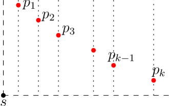
Figure 5: Illustrating the gateways of $V(s)$ and the cut-lines containing them.

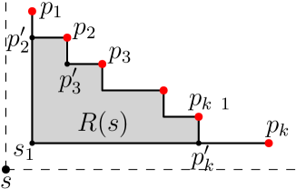
Figure 6: Illustrating the gateway region $R(s)$, which is the shaded region plus $\overline{p_{1}p_{2}^{\prime}}$ and $\overline{p_{k}p_{k}^{\prime}}$. The red points are gateways of $V(s)$.

We use $\beta_{s}$ to denote the boundary portion of $R(s)$ from $p_{1}$ to $p_{k}$ that contains all gateways of $V(s)$. We call $\beta_{s}$ the ceiling, $\overline{s_{1}p_{2}^{\prime}}$ the left boundary, and $\overline{s_{1}p_{k}^{\prime}}$ the bottom boundary of $R(s)$. We refer to the region $R(s)$ excluding the points on $\beta_{s}$ as the interior of $R(s)$.

Observation 1

$R(s)$ is in $\mathcal{P}$, and the interior of $R(s)$ does not contain any polygon vertex of $\mathcal{P}$.

Proof

The lemma can be proved by similar techniques as in [7] (e.g., Lemmas 3.7 and 3.8). However, since the definition in [7] is particularly for (weighted) rectilinear polygonal domains, we present our own proof here, and this also makes our paper more self-contained.

For each $i\in[2,k-1]$, define $w_{i}$ to be the intersection of the vertical line through $p_{i}$ and the horizontal line through $s$ (e.g., see Fig. 7).

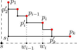
Figure 7: Illustrating the definition of $w_{i}$.

Consider the rectangle $R(w_{i-1},p_{i})$ with $\overline{w_{i-1}p_{i}}$ as a diagonal. Since $p_{i-1}$ and $p_{i}$ are gateways of $V(s)$, both of them are vertically visible to the horizontal line through $s$, and thus, $\overline{p_{i-1}w_{i-1}}$ and $\overline{p_{i}w_{i}}$ are in $\mathcal{P}$. Also because $p_{i-1}$ and $p_{i}$ are gateways of $V(s)$, neither $\overline{p_{i-1}w_{i-1}}\setminus{p_{i-1}}$ nor $\overline{p_{i}w_{i}}\setminus{p_{i}}$ contains any polygon vertex. Further, neither $\overline{p_{i-1}w_{i-1}}$ nor $\overline{p_{i}w_{i}}$ is contained a polygon edge since otherwise the edge would make $s$ not horizontally visible to $l_{k}$, i.e., the cut-line through $p_{k}$. Therefore, we obtain that $\overline{p_{i-1}w_{i-1}}\setminus{p_{i-1}}$ and $\overline{p_{i}w_{i}}\setminus{p_{i}}$ are in the interior of $\mathcal{P}$. Since $s$ is horizontally visible to $l_{k}$, $\overline{w_{i-1}w_{i}}$ is in $\mathcal{P}$. Further, due to our general position assumption $s$ does not have the same $x$- or $y$-coordinate with any polygon vertex, $\overline{w_{i-1}w_{i}}$ is in the interior of $\mathcal{P}$.

We claim that $R(w_{i-1},p_{i})\setminus{\overline{p_{i}^{\prime}p_{i}}}$ does not have a polygon vertex that is vertically visible to $\overline{w_{i-1}w_{i}}$. Assume to the contrary that this is not true, and let $p$ be the lowest such vertex. Since $\overline{p_{i-1}w_{i-1}}\cup\overline{w_{i-1}w_{i}}\cup\overline{p_{i}w_{i}}$ is in $\mathcal{P}$, $p$ must be horizontally visible to $\overline{p_{i-1}w_{i-1}}$. Since $y(p)<y(p_{i}^{\prime})\leq y(p_{i-1})$, $p$ does not define a type-2 Steiner point at the cut-line $l_{i-1}$ since otherwise $p_{i-1}$ would not be a gateway of $s$. Hence, there must be a cut-line $l$ in $\mathcal{T}$ between $p$ and $l_{i-1}$ such that $p$ defines a type-2 Steiner point $p^{\prime}$ on $l$ and $l$ is a proper ancestor of $l_{i-1}$ (and thus prevents $p$ from defining a Steiner point on $l_{i-1}$). Since $l$ is between $p$ and $l_{i-1}$, $s$ is horizontally visible to $l$. As $l_{i-1}$ is a projection cut-line of $s$ and $l$ is an ancestor of $l_{i-1}$, $l$ must also be a projection cut-line of $s$. Further, by the definition of $p$, $p^{\prime}$ is vertically visible to the horizontal line through $s$. This implies that $V(s)$ must have a gateway on $l$ no higher than $p^{\prime}$, and thus the gateway is in $R(w_{i-1},p_{i})\setminus{\overline{p_{i}^{\prime}p_{i}}}$, which incurs contradiction since by definition $R(w_{i-1},p_{i})\setminus\overline{p_{i}^{\prime}p_{i}}$ does not have any gateway of $s$.

The above claim, together with that $\overline{p_{i-1}w_{i-1}}\cup\overline{w_{i-1}w_{i}}\cup\overline{p_{i}w_{i}}$ is in $\mathcal{P}$, leads to that $R(w_{i-1},p_{i})$ is in $\mathcal{P}$. The observation can then be obtained due to the following: (1) $\overline{p_{i-1}w_{i-1}}\cup\overline{p_{i}w_{i}}$ excluding $p_{i-1}$ and $p_{i}$ is in the interior of $\mathcal{P}$, and (2) $R(s)$ is contained in the union of $R(w_{i-1},p_{i})$ for all $i\in[2,k-1]$. ∎

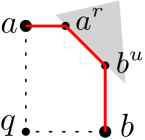
Figure 8: Illustrating the staircase path (the red solid) and the staircase region $R_{s}(a,b)$ (bounded by the solid path and the two dashed segments).

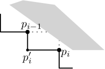
Figure 9: Illustrating the staircase region $R_{s}(p_{i-1},p_{i})$.

For any two points $a$ and $b$ in the plane, we use $R(a,b)$ to denote the rectangle with $\overline{ab}$ as a diagonal. Suppose $a$ and $b$ of $\mathcal{P}$ are both in the first quadrant of $s$ such that $a$ is to the northwest of $b$. Recall that $a^{r}$ denotes the rightward projection of $a$ on $\partial\mathcal{P}$ and $b^{u}$ denotes the upward projection of $b$ on $\partial\mathcal{P}$. With respect to $s$, we say that $a$ and $b$ are in staircase positions if either $\overline{aa^{r}}$ and $\overline{bb^{u}}$ intersect, or both $a^{r}$ and $b^{u}$ are on the same polygon edge (e.g., see Fig. 9); further, in the former case, we call $\overline{ap}\cup\overline{pb}$ the staircase path between $a$ and $b$, where $p=\overline{aa^{r}}\cap\overline{bb^{u}}$, and in the latter case, we call $\overline{aa^{r}}\cup\overline{a^{r}b^{u}}\cup\overline{b^{u}b}$ the staircase path. The region bounded by the staircase path and $\overline{aq}\cup\overline{qb}$, where $q$ is the intersection of the vertical line through $a$ and the horizontal line through $b$, is called the staircase region of $a$ and $b$ with respect to $s$, denoted by $R_{s}(a,b)$. Roughly speaking, $R_{s}(a,b)$ is a pentagon after cutting the upper right corner of $R(a,b)$ by a polygon edge.

Observation 2

For each $i\in[2,k]$, e.g., see Fig. 9, $p_{i-1}$ and $p_{i}$ are in staircase positions and the staircase region $R_{s}(p_{i-1},p_{i})$ is in $\mathcal{P}$. Further, if $y(p_{i-1})>y(p_{i})$, then the interior of $R_{s}(p_{i-1},p_{i})$ along with its left and bottom edges $\overline{p_{i-1}p^{\prime}_{i}}\cup\overline{p_{i}^{\prime}p_{i}}\setminus\{p_{i-1},p_{i}\}$ does not contain a polygon vertex of $\mathcal{P}$.

Proof

The proof is somewhat similar to Observation 1, so we only sketch it. Recall that $y(p_{i-1})\geq y(p_{i})$. If $y(p_{i-1})=y(p_{i})$, then $p_{i-1}=p_{i}^{\prime}$. The proof of Observation 1 shows that $R(w_{i-1},p_{i})$ is in $\mathcal{P}$. Since $\overline{p_{i}^{\prime}p_{i}}$ is the upper edge of $R(w_{i-1},p_{i})$, $R_{s}(p_{i-1},p_{i})=\overline{p_{i}^{\prime}p_{i}}$ is in $\mathcal{P}$ and thus $p_{i-1}$ and $p_{i}$ are in staircase positions.

In the following, we assume that $y(p_{i-1})>y(p_{i})$. As in the proof of Observation 1, $\overline{p_{i-1}p_{i}^{\prime}}\setminus\{p_{i-1}\}$ does not contain any polygon vertex and is in the interior of $\mathcal{P}$. We claim that $R_{s}(p_{i-1},p_{i})$ excluding the top edge and the right edge does not have a polygon vertex that is vertically visible to $\overline{p_{i}^{\prime}p_{i}}$. The proof is similar to that in Observation 1, and we omit the details. The claim, together with $\overline{p_{i-1}p_{i}^{\prime}}\cup\overline{p_{i}^{\prime}p_{i}}\in\mathcal{P}$, leads to the observation. ∎

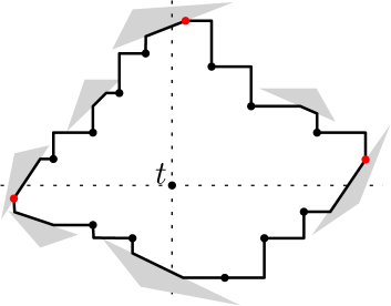
Figure 10: Illustrating the extended gateway region $R(t)$, bounded by the solid segments. The black points other than $t$ are all gateways and the three red points are special gateways to be defined later.

Figure 11: Illustrating the transparent edges on the boundary $R(t)$, shown by the dotted segments. The three red points are special gateways. For illustrating Lemma 1(4), a point $p$ on a transparent edge as well as an endpoint $q$ of the edge is also shown.

3.3 The Extended Gateway Region $R(t)$ for $t$

For $t$, we define an extended gateway region $R(t)$. Unlike $R(s)$, which does not contain $s$, $R(t)$ contains $t$, e.g., see Fig. 11. Before giving the detailed definition of $R(t)$, which is quite lengthy, we first discuss several key properties of it.

An overview of $R(t)$

Let $\mathcal{V}_{1}$ denote the set consisting of all polygon vertices and their projection points on $\partial\mathcal{P}$. In general, $R(t)$ is a simple polygon that contains $t$. Let $\partial R(t)$ denote its boundary. Each edge of $\partial R(t)$ is vertical, horizontal, or on a polygon edge. If an edge of $\partial R(t)$ is not on a polygon edge, then we call it a transparent edge (e.g., see Fig. 11). It is the transparent edges that separate the interior of $R(t)$ from the outside (i.e., for any point $p$ of $\mathcal{P}$ outside $R(t)$, any path from $p$ to $t$ in $\mathcal{P}$ must intersect a transparent edge of $R(t)$). All gateways of $V(t)$ are on $\partial R(t)$. In addition, at most four points of $\mathcal{V}_{1}$ are considered as special gateways that are also on $\partial R(t)$, and we include them in $V(t)$. Then, we have the following lemma (after removing some “redundant” gateways from $V(t)$).

Lemma 1

1. The point $t$ is visible to each gateway in $V(t)$.

2. $R(t)$ is in $\mathcal{P}$.

3. For any point $p$ outside $R(t)$, there is a shortest path from $p$ to $t$ that contains a gateway in $V(t)$, and no shortest path from $p$ to $t$ contains more than one gateway of $V(t)$.

4. For any point $p$ on a transparent edge $e$ of $R(t)$, one of the endpoints $q$ of $e$ is a gateway in $V(t)$ and $\overline{pq}\cup\overline{qt}$ is an $xy$-monotone (and thus a shortest) path from $p$ to $t$ (e.g., see Fig. 11).

5. For any point $p$ on a transparent edge of $R(t)$, if a shortest path $\pi(p,t)$ from $p$ to $t$ contains a gateway $q$ of $V(t)$, then $\overline{pq}$ is in $\pi(p,t)$ and is on a transparent edge $e$ of $R(t)$ (and $q$ is an endpoint of $e$).

Remark.

$R(s)$ and $R(t)$ are defined differently because $s$ and $t$ are not treated symmetrically in our algorithm. For example, we need $R(t)$ to have the properties in Lemma 1, which are not necessary for $R(s)$. Also, as will be clear later, treating $s$ and $t$ differently helps us to further reduce the complexities of our data structure.

In the sequel, we present define $R(t)$ in details, after which we will formally prove Lemma 1.

Let $R_{1}(t)$ be the sub-region of $R(t)$ in the first quadrant of $t$, which is defined as follows (e.g. see Fig. 13). The sub-regions of $R(t)$ in other quadrants are defined similarly.

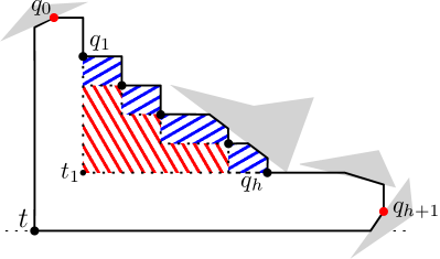
Figure 12: Illustrating $R_{1}(t)$, bounded by the solid segments. The red segments (of negative slope) illustrate $R^{\prime}_{1}(t)$ while the blue segments (of positive slope) show the staircase regions, and their union is $R_{1}^{\prime\prime}(t)$.

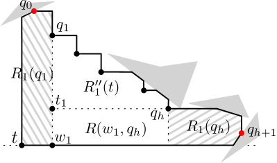
Figure 13: Illustrating the decomposition of $R_{1}(t)$ into four regions: $R^{\prime}_{1}(t)$, $R(w_{1},q_{h})$, and two special regions $R_{1}(q_{1})$ and $R_{1}(q_{h})$, to be defined later. $q_{0}$ and $q_{h+1}$ are two points in $\mathcal{V}_{1}$ to be defined later.

Let $R_{1}^{\prime}(t)$ denote the same gateway region as $R(s)$ for $s$. Let the gateways of $t$ on the ceiling of $R_{1}^{\prime}(t)$ from left to right be $q_{1},q_{2},\ldots,q_{h}$. Let $R_{1}^{\prime\prime}(t)$ denote the union of $R_{1}^{\prime}(t)$ and the staircase regions $R_{t}(q_{i-1},q_{i})$ (with respect to $t$) for all $i\in[2,h]$ (e.g. see Fig. 13). By Observations 1 and 2, $R_{1}^{\prime\prime}(t)$ is in $\mathcal{P}$ and does not contain any polygon vertex except on the boundary portion between $q_{1}$ and $q_{h}$. Let $w_{1}$ denote the intersection of the vertical line through $q_{1}$ and the horizontal line through $t$ (e.g., see Fig. 13). The proof of Observation 1 actually shows that the rectangle $R(w_{1},q_{h})$ is in $\mathcal{P}$ and does not contain contain any polygon vertex except $q_{h}$.

The region $R_{1}(t)$ is the union of $R_{1}^{\prime\prime}(t)$, $R(w_{1},q_{h})$, and two additional regions $R_{1}(q_{1})$ and $R_{1}(q_{h})$, to be defined in the following (e.g., see Fig. 13). In order to define $R_{1}(q_{1})$ and $R_{1}(q_{h})$, we will also need to define two special points $q_{0}$ and $q_{h+1}$ from $\mathcal{V}_{1}$.

3.3.1 The region $R_{1}(q_{1})$

Let $l_{h}(t)$ and $l_{v}(t)$ be the horizontal and vertical lines through $t$, respectively. For a sequence of points $a_{1},a_{2},\ldots,a_{i}$ in the plane, we use $\square(a_{1},a_{2},\ldots,a_{i})$ to denote the polygon with $a_{1},\ldots,a_{i}$ as vertices in this cyclic order on its boundary.

Let $e_{u}$ be the polygon edge that contains the upward projection $t^{u}$ of $t$. Due to our general position assumption, $e_{u}$ is not horizontal. Depending on whether the slope of $e_{u}$ is negative or positive, there are two cases for defining $R_{1}(q_{1})$.

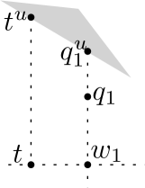
Figure 14: Illustrating the case where the slope of $e_{u}$ is negative.

Figure 15: Illustrating the proof of Observation 3.

Observation 3

If the slope of $e_{u}$ is negative (e.g., see Fig. 15), then the upward projection $q_{1}^{u}$ of $q_{1}$ is on $e_{u}$. Further, the trapezoid $\square(t,w_{1},q_{1}^{u},t^{u})$ is in $\mathcal{P}$ and does not contain any polygon vertex except on $\overline{q_{1}q_{1}^{u}}$.

In this case, we define $R_{1}(q_{1})$ as the above trapezoid.

Proof

Since $q_{1}$ is a gateway, $\overline{w_{1}q_{1}}\setminus\{q_{1}\}$ is in $\mathcal{P}$ and does not contain a polygon vertex.

We claim that no polygon vertex above $t$ and below $t^{u}$ is vertically visible to $\overline{tw_{1}}\setminus\{w_{1}\}$. Indeed, assume to the contrary that this is not true. Then, let $p$ be the lowest such point (e.g., see Fig. 15). Since the slope of $e_{u}$ is negative and $\overline{t^{u}t}\cup\overline{tw_{1}}$ is in $\mathcal{P}$, $p$ must be horizontally visible to $\overline{tt^{u}}$.

By our definition of the graph $G$, there is a cut-line, denoted by $l(p)$, through $p$. Note that $l(p)$ is between $t$ and the cut-line $l(q_{1})$ through $q_{1}$, and $x(p)<x(q_{1})$. Hence, $t$ is horizontally visible to $l(p)$. Depending on whether $l(p)$ is a projection cut-line of $t$, there are two cases.

1. If $l(p)$ is a projection cut-line of $t$, then since $p$ is type-2 Steiner point on $l(p)$ and $p$ is above $t$, $l(p)$ must have a gateway in $V_{g}^{2}(t,G)$ above $t$. But this contradicts with that $q_{1}$ is the leftmost gateway of $V_{g}^{2}(t,G)$ in the first quadrant of $t$.

2. If $l(p)$ is not a projection cut-line of $t$, then there must be a cut-line $l$ in $\mathcal{T}$ that is an ancestor of $l(p)$ such that $l$ is between $t$ and $l(p)$, i.e., $l$ prevents $l(p)$ from being a projection cut-line of $t$. We further let $l$ be such a cut-line in the highest node of $\mathcal{T}$ (i.e., $l$ is still between $t$ and $l(p)$, and is an ancestor of $l(p)$). Then, $l$ must be a projection cut-line of $t$.

   Since $p$ is horizontally visible to $\overline{tt^{u}}$, $p$ is also horizontally visible to $l$ and thus defines a type-2 Steiner point $p^{\prime}$ on $l$ (e.g., see Fig. 15). Clearly, $p^{\prime}$ is vertically visible to the horizontal line $l_{h}(t)$. Therefore, $l$ also has a gateway of $V_{g}^{2}(t,G)$ in the first quadrant of $t$. But this contradicts with that $q_{1}$ is the leftmost gateway of $V_{g}^{2}(t,G)$ in the first quadrant of $t$.

The claim is thus proved. The claim implies that $q_{1}^{u}$ is on $e_{u}$. Further, due to the general position assumption, neither $\overline{t_{u}t}$ nor $\overline{tw_{1}}$ contains a polygon vertex. Recall that $\overline{w_{1}q_{1}}\setminus\{q_{1}\}$ does not have a polygon vertex. Hence, the claim leads to the observation due to $\overline{t_{u}t}\cup\overline{tw_{1}}\cup\overline{w_{1}q_{1}^{u}}$ is in $\mathcal{P}$. ∎

If the slope of $e_{u}$ is positive, we also need to define a point $q_{0}\in\mathcal{V}_{1}$ on $t^{u}$. Depending on whether $y(q_{1})\geq y(t_{u})$, there are two sub-cases.

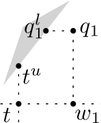
Figure 16: Illustrating the case where the slope of $e_{u}$ is positive and $y(q_{1})\geq y(t^{u})$.

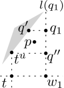
Figure 17: Illustrating the proof of Observation 4.

Observation 4

If the slope of $e_{u}$ is positive and $y(q_{1})\geq y(t_{u})$, e.g., see Fig. 17, then the left projection $q_{1}^{l}$ of $q_{1}$ is on $e_{u}$, and the pentagon $\square(t,w_{1},q_{1},q_{1}^{l},t^{u})$ is in $\mathcal{P}$ and does not contain any polygon vertex except on the top edge $\overline{q_{1}q_{1}^{l}}$.

In this case, we define $q_{0}$ as $q_{1}^{l}$, which must be in $\mathcal{V}_{1}$, and define $R_{1}(q_{1})$ as the above pentagon.

Proof

Let $l(q_{1})$ be the cut-line through $q_{1}$ and let $q^{\prime}$ be the intersection of the horizontal line through $q_{1}$ and the line containing $e_{u}$. We will show that $q^{\prime}=q_{1}^{u}$. Let $q^{\prime\prime}$ be the intersection of $l(q_{1})$ with the horizontal line through $t^{u}$ (e.g. see Fig. 17). Note that $\overline{w_{1}q_{1}}\setminus\{q_{1}\}$ does not contain any type-2 Steiner point.

First of all, by the similar proof as that for Observation 3, we can show that no polygon vertex above $t$ and below $t^{u}$ is vertically visible to $\overline{tw_{1}}\setminus\{w_{1}\}$. This implies that the rectangle $R(t,q^{\prime\prime})$ does not contain any polygon vertex except $q_{1}$ (when $q_{1}=q^{\prime\prime}$), since $\overline{t^{u}t}\cup\overline{tw_{1}}\cup\overline{w_{1}q_{1}}\setminus\{q_{1}\}$ is in $\mathcal{P}$ and does not contain a polygon vertex. This further implies that $R(t,q^{\prime\prime})$ is in $\mathcal{P}$ and does not contain any polygon vertex except possibly $q_{1}$. In the following, we focus on the trapezoid $\square(t^{u},q^{\prime\prime},q_{1},q^{\prime})$, and we let $D$ denote the trapezoid but excluding the top edge $\overline{q^{\prime}q_{1}}$.

We claim that $D$ does not contain any polygon vertex. Assume to the contrary that this is not true. Let $p$ be the lowest such vertex (e.g., see Fig. 17). Then $y(p)<y(q_{1})$, and $p$ is vertically visible to $\overline{tw_{1}}$ and is horizontally visible to $\overline{q_{1}w_{1}}$. Since $q_{1}$ is a gateway, $p$ does not define a Steiner point at $l(p)$. This is only possible when there is a cut-line $l$ in $\mathcal{T}$ that is an ancestor of $l(q_{1})$ and $l$ is between $p$ and $l(q_{1})$ (and $l\neq l(q_{1})$). However, since $l$ is between $t$ and $l(q_{1})$ and $l$ is an ancestor of $l(q_{1})$, $l$ would prevent $l(q_{1})$ from being a projection cut-line of $t$, incurring contradiction.

Since $D$ does not contain any polygon vertex and $\overline{q^{\prime}t^{u}}\cup\overline{t^{u}t}\cup\overline{tw_{1}}\cup\overline{w_{1}q_{1}}\subseteq\mathcal{P}$, the above claim implies that $q^{\prime}$ must be $q_{1}^{l}$.

The above discussion also implies that the union of $\square(t^{u},q^{\prime\prime},q_{1},q^{\prime})$ and $R(t,q^{\prime\prime})$, which is exactly the pentagon in the lemma statement, is in $\mathcal{P}$ and does not contain any polygon vertex except the top edge $\overline{q_{1}q_{1}^{l}}$.

Finally, to see that $q_{0}$ must be a point in $\mathcal{V}_{1}$, let $v$ be the polygon vertex defining the Steiner point $q_{1}$. Then, $q_{0}=q_{1}^{l}$ must be $v^{l}$, which is in $\mathcal{V}_{1}$. ∎

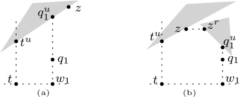
Figure 18: Illustrating the case where the slope of $e_{u}$ is positive and $y(q_{1})<y(t^{u})$: (a) $x(z)\geq x(q_{1})$; (b) $x(z)<x(q_{1})$.

Observation 5

Suppose the slope of $e_{u}$ is positive and $y(q_{1})<y(t_{u})$. Let $z$ be the first point of $\mathcal{V}_{1}$ on $e_{u}$ to the right of $t_{u}$.

1. If $x(z)\geq x(q_{1})$, e.g., see Fig 18(a), then the upward projection $q_{1}^{u}$ of $q_{1}$ must be on $e_{u}$, and the trapezoid $\square(t,w_{1},q_{1}^{u},t^{u})$ is in $\mathcal{P}$ and does not contain any polygon vertex except on $\overline{q_{1}q_{1}^{u}}$.

   In this case, $q_{0}$ is undefined and $R_{1}(q_{1})$ is defined as the trapezoid $\square(t,w_{1},q_{1}^{u},t^{u})$.

2. If $x(z)<x(q_{1})$, e.g., see Fig 18(b), then $z$ and $q_{1}$ are in staircase positions (with respect to $t$), and further, the region bounded by $\overline{zt^{u}}\cup\overline{t^{u}t}\cup\overline{tw_{1}}\cup\overline{w_{1}q_{1}}$ and the staircase path from $q_{1}$ to $z$ is in $\mathcal{P}$ and does not contain any polygon vertex except on the horizontal edge (incident to $z$) and the vertical edge (incident to $q_{1}$) in the staircase path between $z$ and $q_{1}$.

   In this case, we define $q_{0}$ as $z$ and define $R_{1}(q_{1})$ as the region specified above.

Proof

By the similar proof as that for Observation 3, we can show the following claim: No polygon vertex above $t$ and below $t^{u}$ is vertically visible to $\overline{tw_{1}}\setminus\{w_{1}\}$. We also claim that no polygon vertex is horizontally visible to $\overline{t^{u}z}\setminus\{z\}$, since otherwise its leftward projection (which is in $\mathcal{V}_{1}$) would be on $\overline{t^{u}z}\setminus\{z\}$, contradicting with the definition of $z$.

If $x(z)\geq x(q_{1})$, then since $\overline{t^{u}t}\cup\overline{tw_{1}}\cup\overline{w_{1}q_{1}}$ is in $\mathcal{P}$, the above two claims imply that $q_{1}^{u}$ is on $e_{u}$. This further implies that $\square(t^{u},t,w_{1},q_{1}^{u})$ is in $\mathcal{P}$ and does not contain any polygon vertex except on $\overline{q_{1}q_{1}^{u}}$, since $\overline{q_{1}^{u}t^{u}}\cup\overline{t^{u}t}\cup\overline{tw_{1}}\cup\overline{w_{1}q_{1}}\setminus\{q_{1},q_{1}^{u}\}$ does not contain a polygon vertex.

If $x(z)<x(q_{1})$, since $\overline{zt^{u}}\cup\overline{t^{u}t}\cup\overline{tw_{1}}\cup\overline{w_{1}q_{1}}$ is in $\mathcal{P}$, the above two claims imply that $z$ and $q_{1}$ are in staircase positions. As in the above case, this further implies that the region specified in the observation is in $\mathcal{P}$ and does not contain any polygon vertex except on the horizontal edge incident to $z$ and the vertical edge incident to $q_{1}$ in the staircase path between $z$ and $q_{1}$. ∎

3.3.2 The region $R_{1}(q_{h})$

We proceed to define the region $R_{1}(q_{h})$. Let $e_{r}$ be the polygon edge containing the right projection $t^{r}$ of $t$. Let $w_{h}$ be intersection of $l_{h}(t)$ and the vertical line through $q_{h}$. Depending on whether the slope of $e_{r}$ is negative or positive, there are two cases.

Observation 6

If the slope of $e_{r}$ is negative, e.g., see Fig. 20, then the right projection $q_{h}^{r}$ of $q_{h}$ is on $e_{r}$, and the trapezoid $\square(q_{h},w_{h},t^{r},q_{h}^{r})$ is in $\mathcal{P}$ and does not contain any polygon vertex except on the top edge $\overline{q_{h}q_{h}^{r}}$.

In this case, we define $R_{1}(q_{h})$ as the trapezoid $\square(q_{h},w_{h},t^{r},q_{h}^{r})$.

Proof

We first claim that no polygon vertex above $w_{h}$ and strictly below $q_{h}$ is vertically visible to $\overline{w_{h}t^{r}}$. Indeed, assume to the contrary this is not true. Let $p$ be the lowest such vertex. Note that $p$ cannot be on $\overline{q_{h}w_{h}}$ since otherwise $q_{h}$ would not be a gateway of $t$. Let $l(q_{h})$ be the cut-line through $q_{h}$. Since $\overline{q_{h}w_{h}}\cup\overline{w_{h}t^{r}}$ is in $\mathcal{P}$, $p$ must be horizontally visible to $l(q_{h})$. Due to $y(p)<y(q_{h})$ and $q_{h}$ is a gateway of $t$, $p$ cannot define a type-2 Steiner point on $l(q_{h})$. Hence, there is a cut-line $l$ between $p$ and $l(q_{h})$ such that $l$ is an ancestor of $l(q_{h})$ in $\mathcal{T}$. We let $l$ be the highest such ancestor. Hence, $p$ defines a type-2 Steiner point $p^{\prime}$ at $l$. Since $l$ is between $l(q_{h})$ and $t_{r}$, $t$ is horizontally visible to $l$. Since $l$ is an ancestor of $l(q_{h})$ and $l(q_{h})$ is a projection cut-line of $t$, $l$ must be a projection cut-line of $t$. Since $p^{\prime}$ is a type-2 Steiner point vertically visible to $\overline{tt^{r}}$, $l$ also has a gateway of $V_{g}^{2}(t,G)$ above $t$. But this contradicts with that $q_{h}$ is the rightmost gateway of $V_{g}^{2}(t,G)$ in the first quadrant of $t$.

As $\overline{q_{h}w_{h}}\cup\overline{w_{h}t^{r}}$ is in $\mathcal{P}$, the above claim implies that the right projection $q_{h}^{r}$ of $q_{h}$ is on $e_{r}$, and the trapezoid $\square(q_{h},w_{h},t^{r},q_{h}^{r})$ is in $\mathcal{P}$ and does not contain any polygon vertex except on the top edge $\overline{q_{h}q_{h}^{r}}$. ∎

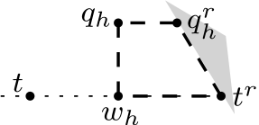
Figure 19: Illustrating the region $R_{1}(q_{h})$ (bounded by the thick dashed segments) in the case where the slope of $e_{r}$ is negative.

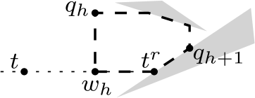
Figure 20: Illustrating the region $R_{1}(q_{h})$ (bounded by the thick dashed segments) in the case where the slope of $e_{r}$ is positive.

Observation 7

If the slope of $e_{r}$ is positive, e.g., see Fig. 20, define $q_{h+1}$ to be the first point of $\mathcal{V}_{1}$ on $e_{r}$ above $t^{r}$.

1. $y(q_{h+1})\leq y(q_{h})$, and the two points $q_{h}$ and $q_{h+1}$ are in staircase positions (with respect to $t$).

2. The region bounded by $\overline{q_{h}w_{h}}\cup\overline{w_{h}t^{r}}\cup\overline{t^{r}q_{h+1}}$ and the staircase path from $q_{h+1}$ to $q_{h}$ is in $\mathcal{P}$, and does not contain any polygon vertex except on the vertical edge (incident to $q_{h+1}$) and the horizontal edge (incident to $q_{h}$) in the staircase path from $q_{h+1}$ to $q_{h}$.

In this case, we define $R_{1}(q_{h})$ as the region specified above.

Proof

Since $q_{h}$ is type-2 Steiner point, its right projection on $\partial\mathcal{P}$ is in $\mathcal{V}_{1}$. Based on this and due to $\overline{q_{h}w_{h}}\cup\overline{w_{h}t^{r}}\subseteq\mathcal{P}$, we can show $y(q_{h+1})\leq y(q_{h})$. The analysis is similar as before and we omit the details.

By the same analysis as in the proof of Observation 6, we can show that no polygon vertex above $w_{h}$ and strictly below $q_{h}$ is vertically visible to $\overline{w_{h}t^{r}}$.

We claim that no polygon vertex above $t_{r}$ and strictly below $q_{h}$ is vertically visible to $\overline{t^{r}q_{h+1}}\setminus\{q_{h+1}\}$. Assume to the contrary this is not true. Let $p$ be such a vertex. Then, the downward projection $p^{d}$ of $p$ is at $\overline{t^{r}q_{h+1}}\setminus\{q_{h+1}\}$. But this contradicts with the definition of $q_{h+1}$ since $p^{d}$ is in $\mathcal{V}_{1}$.

The above two claims, together with $\overline{q_{h}w_{h}}\cup\overline{w_{h}t^{r}}\cup\overline{t^{r}q_{h+1}}$ is in $\mathcal{P}$, lead to that $q_{h}$ and $q_{h+1}$ are in staircase positions and the region specified in the observation is in $\mathcal{P}$. Further, as discussed before, neither $\overline{q_{h}w_{h}}\setminus\{q_{h}\}$ nor $\overline{w_{h}t^{r}}\setminus\{t^{r}\}$ contains a polygon vertex of $\mathcal{P}$. This proves the observation. ∎

3.3.3 A summary of the extended gateway region $R(t)$

The above defined $R_{1}(q_{1})$ and $R_{1}(q_{h})$, and in some cases we also defined $q_{0}$ and $q_{h+1}$, both from $\mathcal{V}_{1}$. We consider $q_{0}$ and $q_{h+1}$ as two special gateways for $t$ and include them in $V(t)$. Note that both $q_{0}$ and $q_{h+1}$ can be computed in additional $O(\log n)$ time.

We perform the following cleanup procedure as part of our query algorithm. If two consecutive gateways $q_{i}$ and $q_{i+1}$ for any $i\in[0,h]$ have the same $x$-coordinate, then we remove $q_{i+1}$ from $V(t)$. The reason is that for any point $p\in\mathcal{P}$ such that a shortest path from $s$ to $p$ contains a $q_{i+1}$, there must be a shortest path from $s$ to $p$ that contains $q_{i}$ because there is a shortest path from $t$ to $q_{i+1}$ that contains $q_{i}$. The cleanup procedure can be done in $O(n_{t})$ time. Without loss of generality, we assume that none of the gateways $q_{0}$ (if exists), $q_{1},q_{2},\ldots,q_{h}$, $q_{h+1}$ (if exists) has been removed by the cleanup procedure since otherwise we could simply re-index them. The following observation follows from our definition of $q_{0}$ and $q_{h+1}$ as well as the cleanup procedure.

Observation 8

The gateways $q_{0}$ (if exists), $q_{1},\ldots,q_{h}$, and $q_{h+1}$ (if exists) are sorted by $x$-coordinate in strictly increasing order and also sorted by $y$-coordinate in strictly decreasing order.

The definition of $R_{1}(t)$ is thus complete. So is the extended gateway region $R(t)$, since sub-regions of $R(t)$ in other quadrants of $t$ are defined similarly. If we store the four projections on $\partial\mathcal{P}$ for each Steiner point of $G$ (this costs $O(n\log n)$ additional space), then $R(t)$ can be explicitly computed in $O(\log n)$ time.

Note that some edges of the boundary of $R(t)$ are on polygon edges, and we call other edges transparent edges (e.g., see Fig. 11). We refer to the outside of $R(t)$ as the points of $\mathcal{P}$ that are either not in $R(t)$ or on the transparent edges. Clearly, for any point $p$ of $\mathcal{P}$ outside $R(t)$, any path from $p$ to $t$ in $\mathcal{P}$ must intersect a transparent edge of $R(t)$.

Lemma 1 given earlier summarizes some properties of $R(t)$ that will be used later in our algorithm. We formally prove it below.

Proof of Lemma 1.

The first and second parts of the lemma can be seen from the definition of $R(t)$ along with Observations 1, 2, 3, 4, 5, 6, and 7.

For the third part, any shortest path $\pi(p,t)$ from $p$ to $t$ must intersect a point at a transparent edge of $R(t)$. Observe that each transparent edge is either horizontal or vertical. Further, for each transparent edge $e$, it always has an endpoint $v$ such that for each point $q\in e$, $\overline{vq}\cup\overline{qt}$ is a $xy$-monotone path from $q$ to $t$, and thus is a shortest path. Therefore, we obtain that there is a shortest path from $p$ to $t$ containing a gateway. On the other hand, assume to the contrary that the path contains two gateways $a$ and $b$ of $V(t)$. Without loss of generality, assume that we meet $a$ first if we move from $p$ to $t$ on the path, and thus $b$ is in the sub-path from $a$ to $t$. This implies that $b$ must be in the rectangle $R(t,a)$ since there is an $xy$-monotone path from $a$ to $t$. However, this is not possible according to our definition of $V(t)$ (in particular, due to the cleanup procedure).

The fourth part follows immediately from the above discussion.

For the fifth part, since there is an $xy$-monotone path from $t$ to $p$, $\pi(p,t)$ must be in the rectangle $R(p,t)$. Thus, $q$ is in $R(p,t)$. According to our definition of $R(t)$, $\overline{pq}$ must be on a transparent edge and $q$ is an endpoint of the edge. Since every transparent edge is either vertical or horizontal, $\overline{pq}$ is either horizontal or vertical, and thus $\overline{pq}$ is the only shortest path from $p$ to $q$. This implies that $\overline{pq}$ is in $\pi(p,t)$. ∎

Figure 21: The following situation cannot occur: A shortest path (the dotted curve) from $t$ to a point $p$ outside $R(t)$ separates the boundary of $R(t)$ (the solid circle) into two disjoint pieces.

Remark.

Lemma 1(5) guarantees that for any point $p$ outside $R(t)$, a shortest path $\pi(p,t)$ cannot separate the boundary of $R(t)$ into two disjoint pieces (e.g., see Fig. 21).

3.4 The Query Algorithm

We have all necessary geometric prerequisites ready for explaining our algorithm.

Consider the gateway region $R(s)$ of $s$. Note that for any $p_{i}\in V(s)$, there is always a shortest path from $s$ to $p_{i}$ containing $s_{1}$ as there is an $xy$-monotone path from $s$ to $s_{1}$ in $\mathcal{P}$. Recall that we have assumed that there exists a shortest $s$-$t$ path that contains a gateway of $V(s)$. The above implies that there exists a shortest path from $s_{1}$ to $t$ that contains a gateway of $V(s)$, and if we can find such a path, by attaching an $xy$-monotone path from $s$ to $s_{1}$ to the path, we can obtain a shortest $s$-$t$ path. For convenience, in the following, we will focus on finding a shortest path from $s_{1}$ to $t$ that contains a gateway of $V(s)$. By slightly abusing the notation, we still use $s$ to represent $s_{1}$. Again, our goal is to find a via gateway of $s$ in $V(s)$.

We first check whether there is a trivial shortest $s$-$t$ path in $O(\log n)$ time. If yes, we are done. Otherwise, we proceed as follows. We begin with the following lemma.

Lemma 2

If $R(t)$ contains a gateway $p$ of $V(s)$, then $\overline{sp}\cup\overline{pt}$ is a shortest $s$-$t$ path; otherwise, $R(s)$ does not intersect $R(t)$.

Proof

Assume that there is a point $p$ that is in both $R(s)$ and $R(t)$. In the following, we first show that $t$ must be in the first quadrant of $p$.

By the definition of $R(s)$, the rectangle $R(s,p)$ is in $R(s)$. For the rectangle $R(t,p)$, it may not be in $R(t)$, but this only happens when one (or both) of its other two corners than $t$ and $p$ is cut by a polygon edge (e.g., see Fig. 23). In particular, we have the following observation: (1) If a point $q\in R(t,p)$ is visible to $p$, then $q$ is also visible to $t$ and there are two trivial shortest paths from $q$ to $t$ whose edges incident to $q$ are vertical and horizontal, respectively (e.g., see Fig. 23).

Note that $t$ cannot be in $R(s)$, since otherwise there would be a trivial shortest $s$-$t$ path, a contradiction. Let $w_{1}$ and $w_{2}$ be the other two corners of $R(p,t)$ such that $p,w_{1},t,w_{2}$ are ordered clockwise on the boundary of $R(p,t)$.

Assume to the contrary that $t$ is not in the first quadrant of $p$. Then, $t$ is in the second, third, or fourth quadrant of $p$. In the following we will show that in each case there is a trivial shortest $s$-$t$ path, which incurs contradiction.

If $t$ is in the second quadrant of $p$, then depending on whether $x(t)\geq x(s)$, there are two subcases.

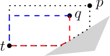
Figure 22: The region bounded by the dotted segments are the region of $R(t,p)$ contained in $R(t)$. The blue and red paths are two trivial shortest paths from $q$ to $t$ whose edges incident to $q$ are vertical and horizontal, respectively.

Figure 23: Illustrating the case where $t$ is in the first quadrant of $p$.

1. If $x(t)\geq x(s)$, then $\overline{pw_{1}}$ must be in $R(s)$. By the above observation, $t$ is visible to $w_{1}$ and thus is vertically visible to the bottom boundary of $R(s)$. This implies that there is a trivial shortest $s$-$t$ path.

2. If $x(t)<x(s)$, then let $w$ be the intersection of $\overline{pw_{1}}$ and the left boundary of $R(s)$. By our above observation, there is a trivial shortest path from $w$ to $t$ such that the edge of the path incident to $w$ is vertical. Since $y(t)\geq y(w)\geq y(s)$, if we append $\overline{sw}$ in front of the above path, we obtain a trivial shortest $s$-$t$ path.

If $t$ is in the third quadrant of $p$, then since $t\not\in R(s)$, $t$ cannot be in the first quadrant of $s$. Depending on which of the other three quadrants of $s$ contains $t$, there are further three subcases.

1. If $t$ is in the second quadrant of $s$, then $w_{1}$ is in $R(s)$ and thus $t$ is visible to $w_{1}$. Hence, $\overline{tw_{1}}$ intersects the left boundary of $R(s)$, implying that there is a trivial shortest $s$-$t$ path.

2. If $t$ is in the third quadrant of $s$, then $s$ is in $R(t,p)$. Since $s$ is visible to $p$, by our above observation, there is a trivial shortest $s$-$t$ path.

3. If $t$ is in the fourth quadrant of $s$, then $w_{2}$ is in $R(s)$ and thus $t$ is visible to $w_{2}$. Hence, $\overline{tw_{2}}$ intersects the bottom boundary of $R(s)$, implying that there is a trivial shortest $s$-$t$ path.

If $t$ is in the fourth quadrant of $p$, then depending on whether $y(t)\geq y(s)$, there are two subcases.

1. If $y(t)\geq y(s)$, then $\overline{pw_{2}}$ is in $R(s)$. By the above observation, $t$ is visible to $w_{2}$ and is thus horizontally visible to the left boundary of $R(s)$. Hence, there is a trivial shortest $s$-$t$ path.

2. If $y(t)<y(s)$, then $\overline{pw_{2}}$ intersects the bottom boundary of $R(s)$, say, at a point $w$. Since $w$ is visible to $p$, by the above observation, there is a trivial shortest path from $w$ to $t$ such that the edge of the path incident to $w$ is horizontal. Since $x(t)\geq x(w)\geq x(s)$, if we append $\overline{sw}$ in front of the above path, we obtain a trivial shortest $s$-$t$ path.

The above proves that $t$ must be in the first quadrant of $p$. Since $s$ is in the third quadrant of $p$, $\overline{sp}\cup\overline{pt}$ is a shortest $s$-$t$ path. This proves the lemma if $R(t)$ contains a gateway $p$ of $V(s)$.

In the following, we assume that $R(t)$ does not contain any gateway of $V(s)$. Our goal is to prove that $R(s)$ does not intersect $R(t)$. Assume to the contrary that this is not true and let $p$ be a point in $R(s)\cap R(t)$. According to the above discussion, $t$ must be in the first quadrant of $p$. In the following, we show that there exists a trivial shortest $s$-$t$ path, which incurs contradiction.

Let $i\in[1,k]$ be the largest index such that $x(p_{i})\leq x(p)$ (e.g., see Fig. 23). Recall that the rightmost point of $R(s)$ is $p_{k}$. Since $R(t)$ does not contain any gateway of $V(s)$, $p$ is not $p_{k}$. This implies that $i<k$, and thus $p_{i+1}$ exists. Depending on whether $x(t)<x(p_{i+1})$, there are two subcases.

1. If $x(t)<x(p_{i+1})$, then $y(t)>y(p_{i+1})$ must hold since otherwise $t$ would be in $R(s)$, e.g., see Fig. 23. This implies that $\overline{pw_{2}}$ must be in $R(s)$. By the above observation, $t$ is visible to $w_{2}$ and thus is vertically visible to the bottom boundary of $R(s)$. This implies that there is a trivial shortest $s$-$t$ path.

2. If $x(t)\geq x(p_{i+1})$, then $y(t)<y(p_{i+1})$ must hold since otherwise $p_{i+1}$ would be in $R(t,p)$ and also in $R(t)$, contradicting with that $R(t)$ does not contain any gateway of $V(s)$. This implies that $\overline{pw_{1}}$ must be in $R(s)$. By the above observation, $t$ is visible to $w_{1}$ and thus is horizontally visible to the left boundary of $R(s)$. This implies that there is a trivial shortest $s$-$t$ path.∎

Our algorithm starts with checking whether $R(t)$ contains a gateway of $V(s)$. This can be done in $O(n_{t}+n_{s})$ time, as follows. We check the four quadrants of $t$ separately. Let $R_{1}(t)$ be $R(t)$ in the first quadrant of $t$. To check whether $R_{1}(t)$ contains a gateway of $V(s)$, we can simply scan the gateways of $V(s)$ and the gateways of $V(t)$ in $R_{1}(t)$ simultaneously from left to right (somewhat like merge sort), which takes $O(n_{t}+n_{s})$ time. We do the same for other quadrants of $t$.

If $R(t)$ contains a gateway of $V(s)$, then by Lemma 2, we have found a shortest $s$-$t$ path. Otherwise, $R(s)$ and $R(t)$ are disjoint and we proceed as follows.

By Lemma 1, for each $p\in V(s)$, $d(p,t)=\min_{q\in V(t)}(d(p,q)+|\overline{qt}|)$, and we call such a gateway $q$ of $V(t)$ minimizing the above value a coupled gateway of $p$ and use $c(p)$ to denote it.

Our algorithm will compute a “candidate” coupled gateway $c^{\prime}(p)$ for every gateway $p$ of $V(s)$ such that if $p\in V(s)$ is a via gateway, then $c(p)=c^{\prime}(p)$. Therefore, once the algorithm is done, the gateway $p$ that minimizes the value $|\overline{sp}|+d(p,c^{\prime}(p))+|\overline{c^{\prime}(p)t}|$ is a via gateway.

For any two points $a$ and $b$ on the ceiling $\beta_{s}$ of $R(s)$, we use $\beta_{s}[a,b]$ to denote the sub-path of $\beta_{s}$ between $a$ and $b$, which is $xy$-monotone. This means that we can compute $d(p_{i},p_{j})=\overline{|p_{i}p_{j}|}$ in constant time for every two gateways $p_{i}$ and $p_{j}$ in $V(s)$.

We consider $V(t)$ as a cyclic list of points in counterclockwise order around $t$ (we use “counterclockwise” since the list of $V(s)=\{p_{1},p_{2},\ldots,p_{k}\}$ are in clockwise order around $s$).

We first compute $c(p_{1})$ in a straightforward manner, i.e., check every gateway of $V(t)$ (since $d(p,q)$ for any $p\in V(s)$ and $q\in V(t)$ is already computed in our preprocessing). This takes $O(n_{t})$ time. We also compute $c(p_{k})$ in the same way. If there are multiple $c(p_{k})$’s, then we let $c(p_{k})$ refer to the first one from $c(p_{1})$ in the counterclockwise order around $t$. Further, if there is more than one $c(p_{1})$ from the current $c(p_{1})$ to $c(p_{k})$ in the counterclockwise order, then we update $c(p_{1})$ to the one closest to $c(p_{k})$. To simplify the notation, let $q_{1}=c(p_{1})$ and $q_{k}=c(p_{k})$. Note that it is possible that $q_{1}=q_{k}$.

The following lemma will be useful for circumventing the “non-ideal” situation depicted in Fig. 4. Its correctness relies on the fact that the ceiling $\beta_{s}$ of $R(s)$ is $xy$-monotone (and thus is a shortest path).

Lemma 3

For any $p_{i}$ of $V(s)$, if $d(p_{1},p_{i})+d(p_{i},q_{1})=d(p_{1},q_{1})$, then $d(p_{1},p_{j})+d(p_{j},q_{1})=d(p_{1},q_{1})$ and $c(p_{j})=q_{1}$ for each $j\in[1,i]$; similarly, if $d(p_{k},p_{i})+d(p_{i},q_{k})=d(p_{k},q_{k})$, then $d(p_{k},p_{j})+d(p_{j},q_{k})=d(p_{k},q_{k})$ and $c(p_{j})=q_{k}$ for each $j\in[i,k]$.

Proof

We only prove the first part of the lemma since the second part is similar.

First of all, since $d(p_{1},p_{i})+d(p_{i},q_{1})=d(p_{1},q_{1})$, there is a shortest path from $p_{1}$ to $q_{1}$ that contains $p_{i}$. Because $\beta_{s}[p_{1},p_{i}]$ is $xy$-monotone, there is a shortest path $\pi(p_{1},q_{1})$ from $p_{1}$ to $q_{1}$ that contains $\beta_{s}[p_{1},p_{i}]$. Since $\beta_{s}[p_{1},p_{i}]$ contains $p_{j}$, $\pi(p_{1},q_{1})$ contains $p_{j}$. Therefore, $d(p_{1},p_{j})+d(p_{j},q_{1})=d(p_{1},q_{1})$ holds.

Next, we prove that $c(p_{j})=q_{1}$. Assume to the contrary that there exists a point $q\in V(t)$ such that $d(p_{j},q)+d(q,t)<d(p_{j},q_{1})+d(q_{1},t)$. Because $\beta_{s}[p_{1},p_{i}]$ is $xy$-monotone and contains $p_{j}$, we have $d(p_{1},p_{i})=d(p_{1},p_{j})+d(p_{j},p_{i})$. Therefore, we can derive the following

$$\begin{split}d(p_{1},q)+d(q,t)&\leq d(p_{1},p_{j})+d(p_{j},q)+d(q,t)\\ &<d(p_{1},p_{j})+d(p_{j},q_{1})+d(q_{1},t)\\ &\leq d(p_{1},p_{j})+d(p_{j},p_{i})+d(p_{i},q_{1})+d(q_{1},t)\\ &=d(p_{1},q_{1})+d(q_{1},t).\end{split}$$ (1)

But this contradicts with that $q_{1}$ is a coupled gateway of $p_{1}$. ∎

Let $a_{1}$ be the largest index $i\in[1,k]$ such that $d(p_{1},p_{i})+d(p_{i},q_{1})=d(p_{1},q_{1})$, which can be computed in $O(a_{1})$ time, as follows. Starting from $i=2$, we simply check whether $d(p_{1},p_{i})+d(p_{i},q_{1})=d(p_{1},q_{1})$, which can be done in $O(1)$ time since $d(p_{1},p_{i})=|\overline{p_{1}p_{i}}|$ can be computed in constant time and $d(p_{i},q_{1})$ has been computed in the preprocessing. If yes, we proceed with $i+1$; otherwise, we stop the algorithm and set $a_{1}=i-1$. We call the above a stair-walking procedure. The correctness is due to Lemma 3.

Similarly, define $b_{k}$ to be the smallest index $i\in[1,k]$ such that $d(p_{k},p_{i})+d(p_{i},q_{k})=d(p_{k},q_{k})$. By a symmetric stair-walking procedure, we can compute $b_{k}$ as well. By Lemma 3, for each $i\in[1,a_{1}]\cup[b_{k},k]$, $c(p_{i})$ is computed. Hence, if $a_{1}\geq b_{k}$, then $c(p)$ for each $p\in V(s)$ is computed and we can finish the algorithm. Otherwise, we proceed as follows.

Our analysis will repeatedly use the following simple observation.

Observation 9

Suppose $p$ and $q$ are two points in a path $\pi$ in $\mathcal{P}$. If the length of the sub-path of $\pi$ between $p$ and $q$ is not equal to $d(p,q)$, then $\pi$ cannot be a shortest path.

Recall that $\pi_{q_{1}}(p_{a_{1}})$ is the shortest path between $q_{1}$ and $p_{a_{1}}$ in the shortest path tree $T(q_{1})$, and $\pi_{q_{k}}(p_{b_{k}})$ is the shortest path in $T(q_{k})$. The following two lemmas present our strategy for dealing with the non-ideal situation in which $\pi_{q_{1}}(p_{a_{1}})$ (resp., $\pi_{q_{k}}(p_{b_{k}})$) goes through the interior of $R(s)$ (e.g., see Fig. 25).

Lemma 4

1. The shortest path $\pi_{q_{1}}(p_{a_{1}})$ contains a point in the interior of $R(s)$ only if its last edge (i.e., the edge incident to $p_{a_{1}}$) intersects the bottom boundary of $R(s)$, in which case the intersection at the bottom boundary of $R(s)$ has $x$-coordinate in $[x(s),x(p_{a_{1}+1})]$.

2. The shortest path $\pi_{q_{k}}(p_{b_{k}})$ contains a point in the interior of $R(s)$ only if its last edge (i.e., the edge incident to $p_{b_{k}}$) intersects the left boundary of $R(s)$, in which case the intersection at the left boundary of $R(s)$ has $y$-coordinate in $[y(s),y(p_{b_{k}-1})]$.

Proof

Note that since $a_{1}<b_{k}\leq k$, $p_{a_{1}+1}$ exists in $V(s)$. So does $p_{b_{k}-1}$. We only prove the first part of the lemma, and the second part can be proved in a similar way. To simplify the notation, let $i=a_{1}$. Let $e$ be the last edge of $\pi_{q_{1}}(p_{a_{1}})$. We assume that $\pi_{q_{1}}(p_{i})$ contains a point $w$ in the interior of $R(s)$.

Figure 24: The shortest path $\pi_{q_{1}}(p_{a_{1}})$ goes through the interior of $R(s)$.

Figure 25: The shaded region is $R(w_{i},p_{i+1})$.

Let $w_{i}$ (resp., $w_{i+1}$) be the intersection of the vertical line through $p_{i}$ (resp, $p_{i+1}$) with the bottom boundary of $R(s)$ (e.g., see Fig. 25). Let $D=R(w_{i},p_{i+1})$. We claim that $w$ must be in $D$. Indeed, assume to the contrary this is not true. Depending on whether $w$ is strictly to the left or right of $D$, there are two cases.

1. If $w$ is strictly to the left of $D$, then $i>1$. By the definition of $i=a_{1}$, $\beta_{s}[p_{1},p_{i}]\cup\pi_{q_{1}}(p_{i})$ is a shortest path from $p_{1}$ to $q_{1}$, which contains $w$. Let $\pi$ represent the subpath of $\beta_{s}[p_{1},p_{i}]\cup\pi_{q_{1}}(p_{i})$ between $p_{1}$ and $w$. Note that $\pi$ contains $p_{i}$. Since there is an $xy$-monotone path in $R(s)$ from $p_{1}$ to $w$, we have $d(p_{1},w)=|\overline{p_{1}w}|$. On the other hand, since $w$ is strictly to the left of $D$, $p_{i}$ is not in $R(p_{1},w)$. This implies that the length of $\pi$ must be larger than $d(p_{1},w)=|\overline{p_{1}w}|$, contradicting with that $\beta_{s}[p_{1},p_{i}]\cup\pi_{q_{1}}(p_{i})$ is a shortest path from $p_{1}$ to $q_{1}$.

2. If $w$ is strictly to the right of $D$, then there is an $xy$-monotone path from $p_{i}$ to $w$ that contains $p_{i+1}$ and the path is contained in a shortest path from $p_{i}$ to $q_{1}$. Hence, $d(p_{i},q_{1})=d(p_{i},p_{i+1})+d(p_{i+1},q_{1})$. Since $d(p_{1},q_{1})=d(p_{1},p_{i})+d(p_{i},q_{1})$, we obtain that $d(p_{1},q_{1})=d(p_{1},p_{i})+d(p_{i},p_{i+1})+d(p_{i+1},q_{1})=d(p_{1},p_{i+1})+d(p_{i+1},q_{1})$. But this contradicts with the definition of $i=a_{1}$.

The above proves that $w$ must be in $D$. Observe that $d(p_{i},w)=|\overline{p_{i}w}|$. Further, due to Observations 1 and 2, $p_{i}$ is visible to $w$. By Observation 1 and due to $R(s)\cap R(t)=\emptyset$, the endpoint of $e$ other than $p_{i}$, which is a polygon vertex or $q_{1}$, is not in $R(s)$. Hence, $w$ must be contained in $e$ and $e$ must intersect the bottom boundary of $R(s)$. Further, according to the above claim, every point $w\in e\cap R(s)$ must be in $D$, and thus, the intersection of $e$ and the bottom boundary of $R(s)$ must be in $D$. This proves the lemma. ∎

Lemma 5

If the last edge of $\pi_{q_{1}}(p_{a_{1}})$ intersects the bottom boundary of $R(s)$, or the last edge of $\pi_{q_{1}}(p_{b_{k}})$ intersects the left boundary of $R(s)$, then $p_{j}$ for each $j\in[a_{1}+1,b_{k}-1]$ cannot be a via gateway.

Proof

We only prove the case for $\pi_{q_{1}}(p_{a_{1}})$ since the other case is similar. To simplify the notation, let $i=a_{1}$. Let $e$ be the last edge of $\pi_{q_{1}}(p_{a_{1}})$, which intersects the bottom boundary of $R(s)$, say, at a point $w$ (e.g., see Fig. 27). By Lemma 4, $x(w)\in[x(s),x(p_{i+1})]$. Consider any $j\in[a_{1}+1,b_{k}-1]$. In the following, we show that $p_{j}$ cannot be a via gateway. Since $j<b_{k}\leq k$, $y(p_{j})>y(p_{k})=y(s)=y(w)$.

Figure 26: Illustrating the proof of Lemma 5. The red edge $e$ is the last edge in $\pi_{q_{1}}(p_{i})$. The blue dashed path is the subpath of $\pi(s,t)$ between $s$ and $p_{j}$.

Figure 27: This following situation cannot occur: The path $\pi_{q_{1}}(p_{a_{1}})$ (the dotted curve) separates the boundary of $R(t)$ (the solid circle) into two (or more) disconnected pieces.

Assume to the contrary that $p_{j}$ is a via gateway. Then there is a shortest $s$-$t$ path $\pi(s,t)$ that contains $p_{j}$. Without loss of generality, we assume that the sub-path of $\pi(s,t)$ between $s$ and $p_{j}$, denoted by $\pi(s,p_{j})$, consists of a vertical segment through $s$ and a horizontal segment through $p_{j}$ (e.g., see Fig. 27). Since $j>i$ and $x(w)\in[x(s),x(p_{i+1})]$, $e$ intersects the horizontal segment of $\pi(s,p_{j})$ at a point $w^{\prime}$ and $x(w^{\prime})\in[x(s),x(p_{i+1})]$. Note that $y(w^{\prime})>y(w)=y(s)$ since $y(p_{j})>y(s)$. As $c(p_{i})=q_{1}$, $\pi_{q_{1}}(p_{i})\cup\overline{q_{1}t}$ is a shortest path from $p_{i}$ to $t$. Hence, the sub-path of $\pi_{q_{1}}(p_{i})\cup\overline{q_{1}t}$ between $w^{\prime}$ and $t$ is a shortest path from $w^{\prime}$ to $t$. Also, as $w^{\prime}\in\pi(s,t)$, the sub-path of $\pi(s,t)$ between $w^{\prime}$ and $t$ is also a shortest path from $w^{\prime}$ to $t$. Therefore, the concatenation of $\pi_{1}$ and $\pi_{2}$, denoted by $\pi$, is also a shortest $s$-$t$ path, where $\pi_{1}$ is the sub-path of $\pi(s,p_{j})$ between $s$ and $w^{\prime}$ and $\pi_{2}$ is the sub-path of $\pi_{q_{1}}(p_{i})\cup\overline{q_{1}t}$ between $w^{\prime}$ and $t$. Notice that $\pi$ contains $s$, $w^{\prime}$, and $w$ in this order. Since $y(w^{\prime})>y(s)=y(w)$, the length of the subpath between $s$ and $w$ is strictly larger than $d(s,w)=|\overline{sw}|$. However, this contradicts with that $\pi$ is a shortest $s$-$t$ path. Hence, $p_{j}$ cannot be a via gateway. The lemma thus follows. ∎

Due to our preprocessing, we check in constant time whether the last edge of $\pi_{q_{1}}(p_{a_{1}})$ intersects the bottom boundary of $R(s)$. Similarly, we can check whether the last edge of $\pi_{q_{1}}(p_{b_{k}})$ intersects the left boundary of $R(s)$. If the answer is yes for either case, then by Lemma 5, we can stop the algorithm (i.e., no need to compute the coupled gateways for any $p_{i}$ with $i\in[a_{1}+1,b_{k}-1]$). Otherwise, by Lemma 4, neither $\pi_{q_{1}}(p_{a_{1}})$ nor $\pi_{q_{1}}(p_{b_{k}})$ contains a point in the interior of $R(s)$. Thus, the situation depicted in Fig. 25 does not happen to either path. Our algorithm proceeds as follows.

Due to the properties of $R(t)$ in Lemma 1, the following lemma shows that $\pi_{q_{1}}(p_{a_{1}})$ (resp., $\pi_{q_{k}}(p_{b_{k}})$) cannot separate the boundary of $R(t)$ into two disconnected pieces (e.g., see Fig. 27).

Lemma 6

The path $\pi_{q_{1}}(p_{a_{1}})$ (resp., $\pi_{q_{k}}(p_{b_{k}})$) does not contain any point in the interior of $R(t)$, and thus, the intersection of the path with $\partial R(t)$ is connected. Further, $q_{1}$ is the only gateway of $V(t)$ in $\pi_{q_{1}}(p_{a_{1}})$, and similarly, $q_{k}$ is the only gateway of $V(t)$ in $\pi_{q_{k}}(p_{b_{k}})$.

Proof

We only discuss the case for $\pi_{q_{1}}(p_{a_{1}})$, since the case for the other path is similar.

Assume to the contrary that $\pi_{q_{1}}(p_{a_{1}})$ contains a point $w$ in the interior of $R(t)$. Then, the subpath from $p_{a_{1}}$ to $w$ must intersect a transparent edge of $R(t)$ at a point $p$ (e.g., see Fig. 27). Let $\pi=\pi_{q_{1}}(p_{a_{1}})\cup\overline{q_{1}t}$. Since $\pi$ is a shortest path from $p_{a_{1}}$ to $t$, $q_{1}$ must be in the rectangle $R(t,p)$. By Lemma 1(5), the subpath of $\pi$ from $p$ to $q_{1}$ must be the line segment $\overline{q_{1}t}$, which is on $\partial R(t)$. However, this contradicts with that the subpath of $\pi$ from $p$ to $q_{1}$ contains a point $w$ in the interior of $R(t)$. Further, since $\pi$ is a shortest path, by Lemma 1(3), $\pi$ only contains a single gateway of $V(t)$. Hence, $q_{1}$ is the only gateway of $V(t)$ in $\pi_{q_{1}}(p_{a_{1}})$. ∎

Recall that $q_{1}=q_{k}$ is possible. Depending on whether $q_{1}=q_{k}$, there are two cases. In the following, we first describe our algorithm for the unequal case $q_{1}\neq q_{k}$, and later we will show that the equal-case $q_{1}=q_{k}$ can be reduced to the unequal case.

3.4.1 The unequal case $q_{1}\neq q_{k}$

Since $q_{1}\neq q_{k}$, $q_{1}$ and $q_{k}$ partition the cyclic list $V(t)$ into two sequential lists, one of which has $q_{1}$ as the first point and $q_{k}$ as the last point following the counterclockwise order around $t$, and we use $V_{t}(1,k)$ to denote that list. The following observation follows from our definitions of $q_{1}$ and $q_{k}$.

Observation 10

Suppose $q$ is a gateway in $V_{t}(1,k)$.

1. If $q\neq q_{1}$, then $d(p_{1},q_{1})+d(q_{1},t)<d(p_{1},q)+d(q,t)$, which further implies that $d(p_{a_{1}},q_{1})+d(q_{1},t)<d(p_{a_{1}},q)+d(q,t)$.

2. if $q\neq q_{k}$, then $d(p_{k},q_{k})+d(q_{k},t)<d(p_{k},q)+d(q,t)$, which further implies that $d(p_{b_{k}},q_{k})+d(q_{k},t)<d(p_{b_{k}},q)+d(q,t)$.

Proof

We only prove the first part of the observation, since the second part is similar. By the definitions of $q_{1}$ and $q_{k}$, we can immediately obtain that $d(p_{1},q_{1})+d(q_{1},t)<d(p_{1},q)+d(q,t)$. Further, by the definition of $a_{1}$, $d(p_{1},q_{1})=d(p_{1},p_{a_{1}})+d(p_{a_{1}},q_{1})$. On the other hand, it holds that $d(p_{1},q)\leq d(p_{1},p_{a_{1}})+d(p_{a_{1}},q)$. The above three inequalities together lead to $d(p_{a_{1}},q_{1})+d(q_{1},t)<d(p_{a_{1}},q)+d(q,t)$. ∎

For any $i$ and $j$ with $1\leq i\leq j\leq k$, we use the interval $[i,j]$ to represent the gateways $p_{i},p_{i+1},\ldots,p_{j}$. Our algorithm works on the interval $[1,k]$ and $V_{t}(1,k)$. Since $q_{1}\neq q_{k}$, we have the following lemma.

Lemma 7

The two paths $\pi_{q_{1}}(p_{a_{1}})$ and $\pi_{q_{k}}(p_{b_{k}})$ do not intersect.

Proof

Since $q_{1}\neq q_{k}$, by Observation 10, $d(p_{a_{1}},q_{1})+d(q_{1},t)<d(p_{a_{1}},q_{k})+d(q_{k},t)$. Assume to the contrary that $\pi_{q_{1}}(p_{a_{1}})$ and $\pi_{q_{k}}(p_{b_{k}})$ intersect, say, at a point $w$ (e.g., see Fig. 29).

Let $\pi_{1}$ be the path $\pi_{q_{1}}(p_{a_{1}})\cup\overline{q_{1}t}$ and let $\pi_{2}$ be the path $\pi_{q_{k}}(p_{b_{k}})\cup\overline{q_{k}t}$. Let $\pi_{1}^{\prime}$ be the sub-path of $\pi_{1}$ between $w$ and $t$. Let $\pi_{2}^{\prime}$ be the sub-path of $\pi_{2}$ between $w$ and $t$.

If we replace $\pi_{1}^{\prime}$ by $\pi_{2}^{\prime}$ in $\pi_{1}$, we obtain a path $\pi_{3}$ from $p_{a_{1}}$ to $t$ that contains $q_{k}$, and the length of $\pi_{3}$ is at least $d(p_{a_{1}},q_{k})+d(q_{k},t)$. Since $d(p_{a_{1}},q_{1})+d(q_{1},t)<d(p_{a_{1}},q_{k})+d(q_{k},t)$, the length of $\pi_{3}$ is larger than that of $\pi_{1}$. This further implies $|\pi_{1}^{\prime}|$ (i.e., the length of $\pi_{1}^{\prime}$) is smaller than $|\pi_{2}^{\prime}|$.

Now if we replace $\pi_{2}^{\prime}$ by $\pi_{1}^{\prime}$ in $\pi_{2}$, then we obtain another path $\pi_{4}$ from $p_{b_{k}}$ to $t$ that contains $q_{1}$. Since $|\pi_{1}^{\prime}|<|\pi_{2}^{\prime}|$, we obtain that $|\pi_{4}|<|\pi_{2}|$. As $d(p_{b_{k}},q_{1})+d(q_{1},t)\leq|\pi_{4}|$, we have $d(p_{b_{k}},q_{1})+d(q_{1},t)<|\pi_{2}|=d(p_{b_{k}},q_{k})+d(q_{k},t)$. However, this contradicts with the definition of $q_{k}$. ∎

Figure 28: Illustrating the proof of Lemma 7. The two paths $\pi_{q_{1}}(p_{a_{1}})$ and $\pi_{q_{k}}(p_{b_{k}})$ intersect at $w$.

Figure 29: The region bounded by the sold curves is $D^{\prime}$. The (blue) bold dashed boundary portion of $\partial R(t)$ is $B_{t}(1,k)$.

Lemma 9 shows why we need the list $V_{t}(1,k)$, and its proof will need Lemma 8, which shows an important property of a shortest $s$-$t$ path.

Lemma 8

Suppose $\pi(s,t)$ is a shortest path that contains a gateway $p\in V(s)$. Then, the sub-path of $\pi(s,t)$ between $p$ and $t$ does not contain any interior point of $R(s)$.

Proof

Let $\pi(p,t)$ be the subpath of $\pi(s,t)$ from $p$ to $t$. Assume to the contrary that $\pi(p,t)$ contains a point $w$ in the interior of $R(s)$. Then, by Observation 1, $d(s,w)=|\overline{sw}|$. Therefore, the length of the subpath of $\pi(s,t)$ between $s$ and $w$, which contains $p$, is equal to $|\overline{sw}|$. This is possible only if $p$ is in the rectangle $R(s,w)$. Since $w$ is in the interior of $R(s)$, all points of $R(s,w)$ are in the interior of $R(s)$. However, by definition, the gateway $p$, which is on the ceiling of $R(s)$, is not in the interior of $R(s)$. Therefore, $p$ cannot be in $R(s,w)$. This incurs contradiction. ∎

Lemma 9

For any gateway $p_{j}$ with $j\in[a_{1}+1,b_{k}-1]$, if $p_{j}$ is a via gateway, then it has a coupled gateway in $V_{t}(1,k)$.

Proof

Suppose $p_{j}$ is a via gateway with $j\in[a_{1}+1,b_{k}-1]$. Thus, there is a shortest $s$-$t$ path that contains $p_{j}$, and we let $\pi(p_{j},t)$ denote the sub-path from $p_{j}$ to $t$.

If $\pi(p_{j},t)$ intersects the path $\pi_{q_{1}}(p_{a_{1}})$, say, at a point $w$, then we claim that $q_{1}$ is coupled gateway of $p_{j}$. Indeed, observe that $q_{1}$ is a gateway $q$ in $V(t)$ that minimizes the value $d(w,q)+d(q,t)$. Since $\pi(p_{j},t)$ contains $w$, $q_{1}$ is also a gateway $q$ in $V(t)$ that minimizes the value $d(p_{j},q)+d(q,t)$. Thus, $q_{1}$ is a coupled gateway of $p_{j}$. As $q_{1}\in V_{t}(1,k)$, the lemma holds.

If $\pi(p_{j},t)$ intersects the path $\pi_{q_{k}}(p_{b_{k}})$, then by the similar analysis as above, $q_{k}$ is a coupled gateway of $p_{j}$. As $q_{k}\in V_{t}(1,k)$, the lemma also holds for this case.

In the following, we assume that $\pi(p_{j},t)$ does not intersect either $\pi_{q_{1}}(p_{a_{1}})$ or $\pi_{q_{k}}(p_{b_{k}})$.

By Lemma 7, $\pi_{q_{1}}(p_{a_{1}})$ and $\pi_{q_{k}}(p_{b_{k}})$ do not intersect. Recall that neither path contains an interior point of $R(s)$. Hence, $\pi_{q_{1}}(p_{a_{1}})$, $\pi_{q_{k}}(p_{b_{k}})$, $\overline{q_{1}t}$, $\overline{q_{k}t}$, and $\beta_{s}[p_{a_{1}},p_{b_{k}}]$ together form a closed curve that divides the plane into two regions (e.g., see Fig. 29), one of which (denoted by $D^{\prime}$) does not contain $s$. Let $B_{t}(1,k)$ be the boundary portion of $R(t)$ contained in $D^{\prime}$. Lemma 6 implies that the set of gateways of $V(t)$ on $B_{t}(1,k)$ is exactly $V_{t}(1,k)$. Further, $B_{t}(1,k)$ divides $D^{\prime}$ into two subregions: one of them, denoted by $D(1,k)$, contains $\beta_{s}[p_{a_{1}},p_{b_{k}}]$ (and thus contains $p_{j}$), and the other contains $t$ (e.g., see Fig. 29).

By Lemma 8, $\pi(p_{j},t)$ does not contain any point in the interior of $R(s)$. Since $p_{j}$ is in $D(1,k)$ and $t$ is not, and $\pi(p_{j},t)$ does not intersect either $\pi(p_{a_{1}},q_{1})$ or $\pi(p_{b_{k}},q_{k})$, $\pi(p_{j},t)$ must intersect $B_{t}(1,k)$. By Lemma 1 and our definition of $B_{t}(1,k)$, for any point $p$ in $B_{t}(1,k)$, $B_{t}(1,k)$ contains a gateway $q$ such that there is an $xy$-monotone path from $p$ to $t$ that contains $q$, and further, $q$ is in $V_{t}(1,k)$ since $V(t)\cap B_{t}(1,k)=V_{t}(1,k)$. Consequently, since $\pi(p_{j},t)$ intersects $B_{t}(1,k)$, we obtain that $V_{t}(1,k)$ has a gateway $q$ such that there is a shortest path from $p_{j}$ to $t$ that contains $q$. This leads to the lemma. ∎

In light of Lemma 9, to compute the candidate coupled gateways for all $p_{i}$ with $i\in[a_{1}+1,b_{k}-1]$, we only need to consider the gateways in $V_{t}(1,k)$. In the following, we work on the problem recursively. We may consider each recursive step as working on a subproblem, denoted by $([i^{\prime},j^{\prime}],[i,j],V_{t}(i,j))$ with $[i^{\prime},j^{\prime}]\subseteq[i,j]\subseteq[1,k]$, where the goal is to find candidate coupled gateways from a sublist $V_{t}(i,j)$ of $V_{t}(1,k)$ for the gateways in $[i^{\prime},j^{\prime}]$, and further, there exist a shortest path from $p_{a_{i}}$ to the first point of $V_{t}(i,j)$ and a shortest path from $p_{b_{j}}$ to the last point of $V_{t}(i,j)$ such that the two paths do not intersect and neither path contains a point in the interior of $R(s)$. Initially, our subproblem is $([a_{1}+1,b_{k}-1],[1,k],V_{t}(1,k))$. We proceed as follows.

If $b_{k}-1=a_{1}+1$, then the interval $[a_{1}+1,b_{k}-1]$ has only one gateway $p$. We simply check all gateways of $V_{t}(1,k)$ to find the point $q$ that minimizes the value $d(p,q)+d(q,t)$ among all $q\in V_{t}(1,k)$, and then return $q$ as the candidate coupled gateway of $p$. The algorithm can stop. Otherwise, we proceed as follows.

Figure 30: Illustrating a schematic view of the indices: $a_{1}$, $b_{m}$, $m$, $a_{m}$, and $b_{k}$.

Let $m=\lfloor(a_{1}+b_{k})/2\rfloor$. We compute a gateway in $V_{t}(1,k)$ that minimizes the value $d(p_{m},q)+d(q,t)$ for all $q\in V_{t}(1,k)$, and in case of a tie, we use $q_{m}^{1}$ and $q_{m}^{2}$ to refer to the first and the last such gateways in $V_{t}(1,k)$, respectively. Let $V_{t}(1,m)$ and $V_{t}(m,k)$ denote the sublists of $V_{t}(1,k)$ from $q_{1}$ to $q_{m}^{1}$ and from $q_{m}^{2}$ to $q_{k}$, respectively. We set one of $q^{1}_{m}$ and $q^{2}_{m}$ as the candidate coupled gateway of $p_{m}$.

Define $a_{m}$ to be the largest index $i\in[m,b_{k}-1]$ such that $d(p_{m},q^{2}_{m})=d(p_{m},p_{i})+d(p_{i},q^{2}_{m})$ and $b_{m}$ the smallest index $i\in[a_{1}+1,m]$ such that $d(p_{m},q^{1}_{m})=d(p_{m},p_{i})+d(p_{i},q^{1}_{m})$. See Fig. 30. We can compute $a_{m}$ and $b_{m}$ by a similar stair-walking procedure as before. According to Lemma 9, by similar proofs as Lemma 3, we can show that for each $i\in[b_{m},m-1]$, if $p_{i}$ is a via gateway, then $q^{1}_{m}$ is a coupled gateway of $p_{i}$, and for each $i\in[m+1,a_{m}]$, if $p_{i}$ is a via gateway, then $q^{2}_{m}$ is a coupled gateway of $p_{i}$. Thus we set $q^{1}_{m}$ as the candidate coupled gateway for each $p_{i}$ with $i\in[b_{m},m-1]$, and set $q^{2}_{m}$ as the candidate coupled gateway for each $p_{i}$ with $i\in[m+1,a_{m}]$.

If $a_{m}=b_{k}-1$ and $b_{m}=a_{1}+1$, then the candidate coupled gateways of all gateways in $[1,k]$ have been computed and we can stop the algorithm. If $a_{m}=b_{k}-1$ but $b_{m}>a_{1}+1$, the candidate coupled gateways of all gateways in $[m,k]$ have been computed, and thus we work recursively on the subproblem $([a_{1}+1,b_{m}-1],[1,k],V_{t}(1,k))$ (note that the size of the first interval is reduced by at least half). Similarly, if $b_{m}=a_{1}+1$ but $a_{m}<b_{k}-1$, then we work recursively on the subproblem $([a_{m}+1,b_{k}-1],[1,k],V_{t}(1,k))$. Otherwise, both $b_{m}>a_{1}+1$ and $a_{m}<b_{k}-1$ hold, and we proceed as follows.

We have the following two lemmas that are similar to Lemmas 4 and 5.

Lemma 10

1. The path $\pi_{q^{2}_{m}}(p_{a_{m}})$ contains a point in the interior of $R(s)$ only if the last edge of the path intersects the bottom boundary of $R(s)$, in which the intersection at the bottom boundary of $R(s)$ has $x$-coordinate in $[x(s),x(p_{a_{m}+1})]$.

2. The path $\pi_{q^{1}_{m}}(p_{b_{m}})$ contains a point in the interior of $R(s)$ only if the last edge of the path intersects the left boundary of $R(s)$, in which case the intersection at the left boundary of $R(s)$ has $y$-coordinate in $[y(s),y(p_{b_{m}-1})]$.

Proof

The proof is similar to that for Lemma 4 and we omit the details. ∎

Lemma 11

1. If the last edge of $\pi_{q^{2}_{m}}(p_{a_{m}})$ intersects the bottom boundary of $R(s)$, then $p_{i}$ cannot be a via gateway for any $i\in[a_{m}+1,b_{k}-1]$.

2. If the last edge of $\pi_{q^{1}_{m}}(p_{b_{m}})$ intersects the left boundary of $R(s)$, then $p_{i}$ cannot be a via gateway for any $i\in[a_{1}+1,b_{m}-1]$.

Proof

The proof is similar to that of Lemma 5, but also relies on Lemma 9. We briefly discuss it below. We only prove the first part of the lemma since the second part is similar. Let $e$ be the last edge of $\pi_{q^{2}_{m}}(p_{a_{m}})$. To simplify the notation, let $i=a_{m}$ and $q=q_{m}^{2}$.

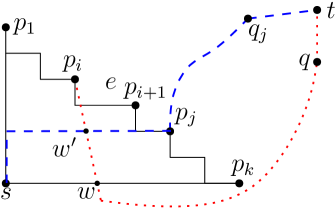
Figure 31: Illustrating the the proof of Lemma 11: The (red) dotted path is $\pi(p_{i},t)$ and the (blue) dashed path is $\pi(s,t)$.

Let $w$ be the intersection of $e$ and the bottom boundary of $R(s)$. By Lemma 10, $x(w)\in[x(s),x(p_{i+1})]$. Assume to the contrary that $p_{j}$ for some $j\in[a_{m}+1,b_{k}-1]$ is a via gateway. Then, by Lemma 9, there must be a shortest $s$-$t$ path $\pi(s,t)$ that contains $\overline{sp_{j}}$ and a gateway of $q_{j}$ in $V_{t}(1,k)$. Without loss of generality, we assume that the sub-path of $\pi(s,t)$ between $s$ and $p_{j}$, denoted by $\pi(s,p_{j})$, consists of a vertical segment through $s$ and a horizontal segment through $p_{j}$ (e.g., see Fig. 31). Then, $\pi(s,p_{j})$ intersects $e$ at a point, say, $w^{\prime}$. Since $j\leq b_{k}-1<k$, $y(p_{j})>y(p_{k})=y(s)$. Thus, $y(w^{\prime})>y(s)$.

Let $\pi(p_{i},t)$ denote the path $\pi_{q}(p_{i})\cup\overline{qt}$, which contains $w^{\prime}$. Recall that $q$ is a gateway in $V_{t}(1,k)$ that minimizes the value $d(p_{i},q^{\prime})+d(q^{\prime},t)$ for all $q^{\prime}\in V_{t}(1,k)$. This implies that $q$ is a gateway in $V_{t}(1,k)$ that minimizes the value $d(w^{\prime},q^{\prime})+d(q^{\prime},t)$ for all $q^{\prime}\in V_{t}(1,k)$. Let $\pi^{\prime}(w^{\prime},t)$ be the subpath of $\pi(p_{i},t)$ between $w^{\prime}$ and $t$.

Let $\pi(w^{\prime},t)$ be the sub-path of $\pi(s,t)$ between $w^{\prime}$ and $t$. Since $\pi(s,t)$ is a shortest $s$-$t$ path, $\pi(w^{\prime},t)$ is also a shortest path from $w^{\prime}$ to $t$. Since $\pi(w^{\prime},t)$ contains a gateway $q_{j}$ in $V_{t}(1,k)$, $q_{j}$ is a gateway in $V_{t}(1,k)$ that minimizes the value $d(w^{\prime},q^{\prime})+d(q^{\prime},t)$ for all $q^{\prime}\in V_{t}(1,k)$. Therefore, the length of $\pi^{\prime}(w^{\prime},t)$ must be the same as that of $\pi(w^{\prime},t)$. Hence, if we replace the subpath $\pi(w^{\prime},t)$ of $\pi(s,t)$ by $\pi^{\prime}(w^{\prime},t)$, we obtain another shortest $s$-$t$ path $\pi^{\prime}(s,t)$.

Notice that the sub-path of $\pi^{\prime}(s,t)$ between $s$ and $w$ is the concatenation of the sub-path of $\pi(s,p_{j})$ from $s$ to $w^{\prime}$ and $\overline{w^{\prime}w}$, whose length is strictly larger than $|\overline{sw}|$ because $y(w^{\prime})>y(s)=y(w)$. However, since $d(s,w)=|\overline{sw}|$, $\pi^{\prime}(s,t)$ cannot be a shortest path. Thus we obtain contradiction. ∎

In constant time we can check whether the two cases in Lemma 11 happen. If both cases happen, then we can stop the algorithm. If the second case happens and the first one does not, then we recursively work on the subproblem $([a_{m}+1,b_{k}-1],[1,k],V_{t}(1,k))$. If the first case happens and the second one does not, then we recursively work on the subproblem $([a_{1}+1,b_{m}-1],[1,k],V_{t}(1,k))$. In the following, we assume that neither case happens. By Lemma 10, neither $\pi_{q^{2}_{m}}(p_{a_{m}})$ nor $\pi_{q^{1}_{m}}(p_{b_{m}})$ contains a point in the interior of $R(s)$. Consequently, we have the following lemma.

Lemma 12

1. For each $i\in[{a_{m}+1},b_{k}-1]$, if $p_{i}$ is a via gateway, then $p_{i}$ has a coupled gateway in $V_{t}(m,k)$. If $q_{m}^{2}\neq q_{k}$, then $\pi_{q_{m}^{2}}(p_{a_{m}})$ does not intersect $\pi_{q_{k}}(p_{b_{k}})$.

2. For each $i\in[{a_{1}+1},b_{m}-1]$, if $p_{i}$ is a via gateway, then $p_{i}$ has a coupled gateway in $V_{t}(1,m)$. If $q_{m}^{1}\neq q_{1}$, then $\pi_{q_{m}^{1}}(p_{b_{m}})$ does not intersect $\pi_{q_{1}}(p_{a_{1}})$.

Proof

We only prove the first part of the lemma, since the second part is similar. Suppose $p_{i}$ is via gateway with $i\in[{a_{m}+1},b_{k}-1]$. Then, there is a shortest $s$-$t$ path $\pi(s,t)$ that contains $p_{i}$, and let $\pi(p_{i},t)$ be the subpath between $p_{i}$ and $t$. By Lemma 8, $\pi(p_{i},t)$ does not contain any interior point of $R(s)$.

We first assume that $q_{m}^{2}\neq q_{1}$. Due to Observation 10, we claim that the path $\pi_{q_{m}^{2}}(p_{a_{m}})$ does not intersect the path $\pi_{q_{1}}(p_{a_{1}})$. Indeed, assume to the contrary that the two paths intersect, say, at the point $w$. Then, by the definitions of $q_{1}$ and $q_{2}^{m}$, each of them is a point in $V_{t}(1,k)$ minimizing the value $d(w,q)+d(q,t)$ for all $q\in V_{t}(1,k)$. This means that $d(p_{a_{1}},q_{1})+d(q_{1},t)=d(p_{a_{1}},q_{m}^{2})+d(q_{m}^{2},t)$. However, this contradicts with Observation 10 since $q_{m}^{2}\neq q_{1}$ and $q_{m}^{2}\in V_{t}(1,k)$.

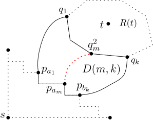
Figure 32: The region bounded by the sold curves is $D(1,k)$, and $\pi_{q_{m}^{2}}(p_{a_{m}})$ (the red dotted curve) partitions it into two subregions, one of which is $D(m,k)$.

Depending on whether $q_{m}^{2}$ is $q_{k}$, there are two cases.

If $q_{m}^{2}\neq q_{k}$, then by the similar proof as above, the path $\pi_{q_{m}^{2}}(p_{a_{m}})$ does not intersect $\pi_{q_{k}}(p_{b_{k}})$ either. Recall that we have defined a region $D(1,k)$ that is bounded by $\beta_{s}[p_{a_{1}},p_{b_{k}}]$, $\pi_{q_{1}}(p_{a_{1}})$, $\pi_{q_{k}}(p_{b_{k}})$, and a boundary portion $B_{t}(1,k)$ of $R(t)$, e.g., see Fig. 32. Recall that $\pi_{q_{m}^{2}}(p_{a_{m}})$ does not intersect the interior of $R(s)$. Since $p_{a_{m}}\in\beta_{s}[p_{a_{1}},p_{b_{k}}]$, $\pi_{q_{m}^{2}}(p_{a_{m}})$ does not intersect either $\pi_{q_{1}}(p_{a_{1}})$ or $\pi_{q_{k}}(p_{b_{k}})$, and $t$ is not in $D(1,k)$, if $w$ is the first point of $\pi_{q_{m}^{2}}(p_{a_{m}})$ on $\partial R(t)$ (such a point $w$ must exists since $q_{m}^{2}$ is on $\partial R(t)$), then $w$ must be on $B_{t}(1,k)$. By our way of defining $B_{t}(1,k)$ and according to Lemma 1(5), the sub-path of $\pi_{q_{m}^{2}}(p_{a_{m}})$ between $w$ and $q_{m}^{2}$ is $\overline{wq_{m}^{2}}$, which must be on $B_{t}(1,k)$. This implies that $\pi_{q_{m}^{2}}(p_{a_{m}})$ is in $D(1,k)$. Since both endpoints of $\pi_{q_{m}^{2}}(p_{a_{m}})$ are on the boundary of $D(1,k)$, $\pi_{q_{m}^{2}}(p_{a_{m}})$ partitions $D(1,k)$ into two subregions, one of which, denoted by $D(m,k)$, contains $\beta_{s}[p_{a_{m}},p_{b_{k}}]$. Let $B_{t}(m,k)$ denote the portion of $B_{t}(1,k)$ in $D(m,k)$. By definition, $V_{t}(m,k)=V(t)\cap B_{t}(m,k)$. Recall that both $q_{m}^{2}$ and $q_{k}$ are in $V_{t}(m,k)$.

We proceed to show that $V_{t}(m,k)$ contains a coupled gateway of $p_{i}$. If the path $\pi(p_{i},t)$ intersects $\pi_{q_{m}^{2}}(p_{a_{m}})$, then by the similar analysis as before, $q_{m}^{2}$ is a coupled gateway of $p_{i}$. Similarly, if $\pi(p_{i},t)$ intersects $\pi_{q_{k}}(p_{b_{k}})$, then $q_{k}$ is a coupled gateway of $p_{i}$. In the following, we assume that $\pi(p_{i},t)$ does not intersect either path. Recall that the path $\pi(p_{i},t)$ does not contain any interior point of $R(s)$. Since $p_{i}$ is in $\beta_{s}[p_{a_{m}},p_{b_{k}}]$ (and thus is in $D(m,k)$) but $t$ is not in $D(m,k)$, $\pi(p_{i},t)$ must intersect $B_{t}(k,m)$, say, at a point $w$. By our way of defining $B_{t}(1,k)$ and according to Lemma 1, $B_{t}(k,m)$ contains a gateway $q$ such that $\overline{wq}\cup\overline{qt}$ is a shortest path from $w$ to $t$. This implies that $q$ is a coupled gateway of $p_{i}$. Since $q\in B_{t}(m,k)$ and $V_{t}(m,k)=V(t)\cap B_{t}(m,k)$, $q$ is in $V_{t}(m,k)$. The lemma is thus proved.

Next, we consider the case where $q_{m}^{2}=q_{k}$. In this case, $V_{t}(m,k)=\{q_{k}\}$ and our goal is to show that $q_{k}$ is a coupled gateway of $p_{i}$. If we move on $\pi_{q_{m}^{2}}(p_{a_{m}})$ from $p_{a_{m}}$ to $q_{m}^{2}$, let $w$ be the first intersection of $\pi_{q_{m}^{2}}(p_{a_{m}})$ and $\pi_{q_{k}}(p_{b_{k}})$. Let $\pi(p_{a_{m}},w)$ be the sub-path of $\pi_{q_{m}^{2}}(p_{a_{m}})$ between $p_{a_{m}}$ and $w$, and $\pi(p_{b_{k}},w)$ the sub-path of $\pi_{q_{k}}(p_{b_{k}})$ between $p_{b_{k}}$ and $w$. Recall that $\pi_{q_{m}^{2}}(p_{a_{m}})$ does not intersect $\pi_{q_{1}}(p_{a_{1}})$ and does not contain any interior point of $R(s)$. We claim that $\pi(p_{a_{m}},w)$ is contained in the region $D(1,k)$. Indeed, this is obviously true if $\pi(p_{a_{m}},w)$ does not intersect $\partial R(t)$. Otherwise, let $z$ be the first intersection between $\pi(p_{a_{m}},w)$ and $\partial R(t)$. Note that $z$ must be on $B_{t}(1,k)$. According to Lemma 1(5), the sub-path of $\pi_{q_{m}^{2}}(p_{a_{m}})$ between $z$ and $q_{m}^{2}$ must be the segment $\overline{zq_{m}^{2}}$, which is on $B_{t}(1,k)$. This also implies that $w\in\overline{zq_{m}^{2}}$ and $\pi(p_{a_{m}},w)$ is in $D(1,k)$, and further, $\pi(p_{a_{m}},w)$ does not contain any point in the interior of $R(t)$. Let $D$ be the sub-region of $D(1,k)$ bounded by $\pi(p_{a_{m}},w)$, $\pi(p_{b_{k}},w)$, and $\beta_{s}[p_{a_{m}},p_{b_{k}}]$. Clearly, $D$ does not contain $t$.

Now consider the path $\pi(p_{i},t)$. Since $p_{i}\in\beta_{s}[p_{a_{m}},p_{b_{k}}]\subseteq D$, $t\not\in D$, $\pi(p_{i},t)$ does not contain any interior point of $R(s)$, and neither $\pi(p_{a_{m}},w)$ nor $\pi(p_{b_{k}},w)$ contains an interior point of $R(t)$, $\pi(p_{i},t)$ must intersect either $\pi(p_{a_{m}},w)$ or $\pi(p_{b_{k}},w)$ (and thus intersect either $\pi_{q_{m}^{2}}(p_{a_{m}})$ or $\pi_{q_{k}}(p_{b_{k}})$). In either case, by the similar analysis as above, $q_{k}$ ($=q_{m}^{2}$) is a coupled gateway of $p_{i}$. The lemma is thus proved.

The above prove the case where $q_{m}^{2}\neq q_{1}$. If $q_{m}^{2}=q_{1}$, then $V_{t}(m,k)=V_{t}(1,k)$. By Lemma 9, it is trivially true that $p_{i}$ has a coupled gateway in $V_{t}(m,k)$. Further, due to Observation 10, by similar analysis as before, $\pi_{q_{m}^{2}}(p_{a_{m}})$ cannot intersect $\pi_{q_{k}}(p_{b_{k}})$. The lemma thus follows. ∎

Based on Lemma 12, our algorithm proceeds as follows. If $q_{m}^{2}=q_{k}$, then we set $q_{k}$ as the candidate coupled gateway for each $p_{i}$ with $i\in[a_{m}+1,b_{k}-1]$. Otherwise, we call the algorithm recursively on the subproblem $([a_{m}+1,b_{k}-1],[m,k],V_{t}(m,k))$. Similarly, if $q_{m}^{1}=q_{1}$, then we set $q_{1}$ as the candidate coupled gateway for each $p_{i}$ with $i\in[a_{1}+1,b_{m}-1]$. Otherwise, we call the algorithm recursively on the subproblem $([a_{1}+1,b_{m}-1],[1,m],V_{t}(1,m))$.

For the running time, notice that the stair-walking procedure spends $O(1)$ time on finding a coupled gateway for a gateway of $V(s)$. Hence, the overall time of the stair-walking procedure in the entire algorithm is $O(n_{s})$. Consider a subproblem $([i^{\prime},j^{\prime}],[i,j],V_{t}(i,j))$.To solve it, after spending $O(|V_{t}(i,j)|)$ time, we either reduce the problem to another subproblem in which the first interval is at most half the size of $[i^{\prime},j^{\prime}]$ and the third gateway set is still $V_{t}(i,j)$, or reduce it to two sub-problems such that each of them has the first interval at most half the size of $[i^{\prime},j^{\prime}]$ and the third gateway sets of the two sub-problems are two disjoint subsets of $V_{t}(i,j)$. Hence, if we consider the algorithm procedure as a tree structure, the height of the tree is $O(\log n_{s})$ and the total time we spend on each level of the tree is $O(n_{t})$. Therefore, the overall time of the algorithm is $O(n_{s}+n_{t}\log n_{s})$.

3.4.2 The equal case $q_{1}=q_{k}$

For the case $q_{1}=q_{k}$, we will eventually reduce it to the above unequal case. In this case, we will need to determine the relative positions of two shortest paths (e.g., $\pi_{q_{1}}(p_{a_{1}})$ and $\pi_{q_{1}}(p_{b_{k}})$) with respect to $\overline{q_{1}t}$. To this end, we perform the following additional preprocessing.

Recall that we have already computed a shortest path tree $T(q_{1})$ from $q_{1}$ to all vertices of $G$. In addition, we compute a post-order traversal list on $T(q_{1})$ (but excludes the root $q_{1}$) and store the list in a cyclic array $L(q_{1})$. This does not change the preprocessing complexities asymptotically.

Recall that $t$ is visible to $q_{1}$. We want to know the position of $t$ at $L(q_{1})$ if we “insert” $t$ into the tree $T(q_{1})$ (and thus $t$ becomes a leaf). This can be done in $O(\log n)$ time by doing binary search on the children of $q_{1}$ in $T(q_{1})$. After that, given any two vertices $v_{1}$ and $v_{2}$ of $T(q_{1})$, by using $L(q_{1})$, we can determine in constant time whether $\pi_{q_{1}}(v_{1})$ is clockwise from $\pi_{q_{1}}(v_{2})$ with respect to the path $\pi_{q_{1}}(t)=\overline{q_{1}t}$ (similar approach was also used in [26]; for simplicity, we assume that $v_{2}\not\in\pi_{q_{1}}(v_{1})$ and $v_{1}\not\in\pi_{q_{1}}(v_{2})$, which is also the case in our algorithm; we say that $\pi_{q_{1}}(v_{2})$ is clockwise from $\pi_{q_{1}}(v_{1})$ if we meet $\pi_{q_{1}}(v_{1})$ first when topologically rotating $\overline{q_{1}t}$ around $q_{1}$ clockwise; e.g., see Fig. 34).

Figure 33: Illustrating an example in which $\pi_{q_{1}}(v_{2})$ is clockwise from $\pi_{q_{1}}(v_{1})$ with respect to $\overline{q_{1}t}$.

Figure 34: Illustrating the case where $\pi_{q_{1}}(p_{a_{m}})$ is clockwise from $\pi_{q_{1}}(p_{b_{k}})$ with respect to $\overline{q_{1}t}$.

We first check whether $\pi_{q_{1}}(p_{a_{1}})$ is clockwise from $\pi_{q_{1}}(p_{b_{k}})$ with respect to $\overline{q_{1}t}$. If yes, the following lemma implies that we can stop our algorithm by setting $q_{1}$ as a candidate coupled gateway for all $p_{i}$ with $i\in[a_{1}+1,b_{k}-1]$.

Lemma 13

If $\pi_{q_{1}}(p_{a_{1}})$ is clockwise from $\pi_{q_{1}}(p_{b_{k}})$ with respect to $\overline{q_{1}t}$ (e.g., see Fig. 34), then for each $i\in[a_{1}+1,b_{k}-1]$, if $p_{i}$ is a via gateway, then $q_{1}$ is a coupled gateway of $p_{i}$.

Proof

If we move from $p_{a_{1}}$ to $q_{1}$ on $\pi_{q_{1}}(p_{a_{1}})$, let $w$ be the first point of the path that intersects $\pi_{q_{1}}(p_{b_{k}})$. Let $\pi(p_{a_{1}},w)$ denote the subpath of $\pi_{q_{1}}(p_{a_{1}})$ between $p_{a_{1}}$ and $w$, and $\pi(p_{b_{k}},w)$ the subpath of $\pi_{q_{1}}(p_{b_{k}})$ between $p_{b_{k}}$ and $w$. Since neither $\pi_{q_{1}}(p_{a_{1}})$ nor $\pi_{q_{1}}(p_{b_{k}})$ contains any interior point of $R(s)$, $\pi(p_{a_{1}},w)\cup\pi(p_{b_{k}},w)\cup\beta_{s}[p_{a_{1}},p_{b_{k}}]$ forms a closed cycle that divides the plane into two regions. We use $D$ to denote the region that does not contain $s$. Since $\pi_{q_{1}}(p_{a_{1}})$ is clockwise from $\pi_{q_{1}}(p_{b_{k}})$ with respect to $\overline{q_{1}t}$ and $p_{a_{1}}$ is counterclockwise from $p_{b_{k}}$ on $\beta_{s}[p_{a_{1}},p_{b_{k}}]$ with respect to $s$, the region $D$ does not contain $t$. Further, by Lemma 6, $D$ does not contain any interior point of $R(t)$ and contains at most one (i.e., $q_{1}$ if $w=q_{1}$) gateway of $t$.

Suppose $p_{i}$ is a via gateway with $i\in[a_{1}+1,b_{k}-1]$. There is a shortest $s$-$t$ path containing $p_{i}$, and we use $\pi(p_{i},t)$ to denote the subpath between $p_{i}$ and $t$. By Lemma 8, $\pi(p_{i},t)$ does not contain any interior point of $R(s)$. Since $i\in[a_{1}+1,b_{k}-1]$, $p_{i}\in\beta_{s}[p_{a_{1}},p_{b_{k}}]$. As $t\not\in D$, $\pi(p_{i},t)$ must intersect either $\pi(p_{a_{1}},w)$ or $\pi(p_{b_{k}},w)$. In either case, by similar analysis as before (e.g., in Lemma 9), we can show that $q_{1}$ is a coupled gateway of $p_{i}$, and we omit the details. ∎

If $\pi_{q_{1}}(p_{a_{1}})$ is counterclockwise from $\pi_{q_{1}}(p_{b_{k}})$, then we proceed as follows.

Let $m=\lfloor(a_{1}+b_{k})/2\rfloor$. We compute a gateway in $V(t)$ that minimizes the value $d(p_{m},q)+d(q,t)$ for all $q\in V(t)$, and in case of tie, we use $q_{m}^{1}$ to refer to the first one in $V(t)$ in the counterclockwise order from $q_{1}$, and use $q_{m}^{2}$ to refer to the first one in $V(t)$ in the clockwise order from $q_{1}$. We set one of $q^{1}_{m}$ and $q^{2}_{m}$ as the candidate coupled gateway of $p_{m}$. Note that $q_{m}^{1}\neq q_{1}$ if and only if $q_{m}^{2}\neq q_{1}$. Depending on whether $q_{m}^{1}=q_{1}$, there are two cases.

If $q_{m}^{1}\neq q_{1}$ (and thus $q_{m}^{2}\neq q_{2}$), then we apply our algorithm for the above unequal case on $[1,m]$ and the gateways of $V(t)$ from $q_{1}$ to $q_{m}^{1}$ in the counterclockwise order. We also apply the algorithm on $[m,k]$ and the gateways of $V(t)$ from $q_{k}$ to $q_{m}^{2}$ in the clockwise order. Therefore, in this case, we have reduced our problem to the unequal case.

If $q_{m}^{1}=q_{1}$, then $q_{m}^{2}=q_{1}$. In this case, we work on the problem for the equal case recursively until the subproblems are reduced to the unequal case (and then we apply the unequal case algorithm). Each recursive step works on a subproblem, denoted by $([i^{\prime},j^{\prime}],[i,j],V(t))$ with $[i^{\prime},j^{\prime}]\subseteq[i,j]\subseteq[1,k]$, where we want to find the candidate coupled gateways in the interval $[i^{\prime},j^{\prime}]$, $q_{1}$ is a coupled gateway for both $p_{a_{i}}$ and $p_{b_{j}}$, and $\pi_{q_{1}}(p_{a_{i}})$ is counterclockwise from $\pi_{q_{1}}(p_{b_{j}})$. Initially, our subproblem is $([a_{1}+1,b_{k}-1],[1,k],V(t))$. We proceed as follows.

Define $a_{m}$ and $b_{m}$ in the same way as before in the unequal case. Similarly as before, if $a_{m}=b_{k}-1$ but $b_{m}>a_{1}+1$, the candidate coupled gateways of $p_{i}$ for all $i\in[m,k]$ have been computed, and thus we work recursively on the subproblem $([a_{1}+1,b_{m}-1],[1,k],V(t))$; if $b_{m}=a_{1}+1$ but $a_{m}<b_{k}-1$, then we work recursively on the subproblem $([a_{m}+1,b_{k}-1],[1,k],V(t))$. Otherwise both $b_{m}>a_{1}+1$ and $a_{m}<b_{k}-1$ hold, and we proceed as follows.

Note that Lemmas 10 and 11 still hold. In constant time we can check whether the two cases in Lemma 11 happen. If both cases happen, then we can stop the algorithm. If the second case happens but the first one does not, then we recursively work on the subproblem $([a_{m}+1,b_{k}-1],[1,k],V(t))$. If the first case happens but the second one does not, then we recursively work on the subproblem $([a_{1}+1,b_{m}-1],[1,k],V(t))$. In the following, we assume that neither case happens. By Lemma 10, neither $\pi_{q_{1}}(p_{a_{m}})$ nor $\pi_{q_{1}}(p_{b_{m}})$ contains a point in the interior of $R(s)$.

Figure 35: Illustrating the case where $\pi_{q_{1}}(p_{a_{m}})$ is clockwise from $\pi_{q_{1}}(p_{b_{k}})$ with respect to $\overline{q_{1}t}$.

In constant time, we further check whether $\pi_{q_{1}}(p_{a_{m}})$ is clockwise from $\pi_{q_{1}}(p_{b_{k}})$ with respect to $\overline{q_{1}t}$. We have the following lemma.

Lemma 14

Let $\pi$ be either $\pi_{q_{1}}(p_{a_{m}})$ or $\pi_{q_{1}}(p_{b_{m}})$. If $\pi$ is clockwise from $\pi_{q_{1}}(p_{b_{k}})$ with respect to $\overline{q_{1}t}$ (e.g., see Fig. 35), then for each $i\in[{a_{m}+1},b_{k}-1]$, if $p_{i}$ is a via gateway, then $q_{1}$ is a coupled gateway of $p_{i}$. Otherwise, for each $i\in[{a_{1}+1},b_{m}-1]$, if $p_{i}$ is a via gateway, then $q_{1}$ is a coupled gateway of $p_{i}$.

Proof

We only prove the case where $\pi$ is $\pi_{q_{1}}(p_{a_{m}})$, since the other case is similar.

Note that $\pi_{q_{1}}(p_{a_{1}})$ and $\pi_{q_{1}}(p_{b_{k}})$ do not cross each other because they are paths in the shortest tree $T(q_{1})$. Since neither $\pi_{q_{1}}(p_{a_{1}})$ nor $\pi_{q_{1}}(p_{b_{k}})$ contains any interior point of $R(s)$, the two paths along with $\beta[p_{a_{1}},p_{b_{k}}]$ form a closed cycle that divides the plane into two regions, one of which (denoted by $D$) does not contain $s$. Since $\pi_{q_{1}}(p_{a_{1}})$ is counterclockwise from $\pi_{q_{1}}(p_{b_{k}})$ with respect to $\overline{q_{1}t}$, $p_{a_{1}}$ is counterclockwise from $p_{b_{k}}$ on $\beta_{s}[p_{a_{1}},p_{b_{k}}]$ with respect to $s$, and neither $\pi_{q_{1}}(p_{a_{1}})$ nor $\pi_{q_{1}}(p_{b_{k}})$ contains any interior point of $R(t)$ (by Lemma 6), $D$ contains $R(t)$.

Recall that $\pi_{q_{1}}(p_{a_{m}})$ does not contain any interior point of $R(s)$. Also, $\pi_{q_{1}}(p_{a_{m}})$ does not cross either $\pi_{q_{1}}(p_{a_{1}})$ or $\pi_{q_{1}}(p_{b_{k}})$ since they are paths in the shortest path tree $T(q_{1})$. Since both endpoints of $\pi_{q_{1}}(p_{a_{m}})$ are on the boundary of $D$, $\pi_{q_{1}}(p_{a_{m}})$ partitions $D$ into two subregions (e.g., see Fig. 35): One subregion, denoted by $D_{1}$, is bounded by $\pi_{q_{1}}(p_{a_{m}})$, $\pi_{q_{1}}(p_{a_{1}})$, and $\beta_{s}[p_{a_{1}},p_{a_{m}}]$, and the other, denoted by $D_{2}$, is bounded by $\pi_{q_{1}}(p_{a_{m}})$, $\pi_{q_{1}}(p_{b_{k}})$, and $\beta_{s}[p_{a_{m}},p_{b_{k}}]$. In addition, by the similar analysis, we can show that Lemma 6 also applies to the path $\pi_{q_{1}}(p_{a_{m}})$.

If $\pi_{q_{1}}(p_{a_{m}})$ is clockwise from $\pi_{q_{1}}(p_{b_{k}})$ with respect to $\overline{q_{1}t}$, then $R(t)$ must be contained in $D_{1}$ (e.g., see Fig. 35). Suppose $p_{i}$ is a via gateway with $i\in[a_{m}+1,b_{k}-1]$. Then, there is a shortest $s$-$t$ path containing $p_{i}$, and we use $\pi(p_{i},t)$ to denote the subpath between $p_{i}$ and $t$. By the same analysis as that in Lemma 13, we can show that $\pi(p_{i},t)$ must intersect either $\pi_{q_{1}}(p_{a_{m}})$ or $\pi_{q_{1}}(p_{b_{k}})$. In either case, $q_{1}$ is a coupled gateway of $p_{i}$.

If $\pi_{q_{1}}(p_{a_{m}})$ is counterclockwise from $\pi_{q_{1}}(p_{b_{k}})$ with respect to $\overline{q_{1}t}$, then $R(t)$ must be contained in $D_{2}$. Then, by similar analysis as above, we can show that for each $i\in[{a_{1}+1},b_{m}-1]\subseteq[{a_{1}+1},a_{m}-1]$, if $p_{i}$ is a via gateway, then $q_{1}$ is a coupled gateway of $p_{i}$. We omit the details. ∎

By Lemma 14, depending on whether $\pi_{q_{1}}(p_{a_{m}})$ is clockwise from $\pi_{q_{1}}(p_{b_{k}})$, there are two cases.

1. If yes, then we set $q_{1}$ as the candidate coupled gateway for all $p_{i}$ with $i\in[{a_{m}+1},b_{k}-1]$. Depending on whether $\pi_{q_{1}}(p_{b_{m}})$ is counterclockwise from $\pi_{q_{1}}(p_{b_{k}})$, there are further two subcases.

   1. If yes, we set $q_{1}$ as the candidate coupled gateway for all $p_{i}$ with $i\in[{a_{1}+1},b_{m}-1]$. Note that we have found the candidate coupled gateways for all $p_{i}$ with $i\in[a_{1}+1,b_{k}-1]$. Hence, we can stop the algorithm.

   2. Otherwise, we recursively work on the subproblem $([a_{1}+1,b_{m}-1],[1,m],V(t))$.

2. If $\pi_{q_{1}}(p_{a_{m}})$ is counterclockwise from $\pi_{q_{1}}(p_{b_{k}})$, then we set $q_{1}$ as the candidate coupled gateway for all $p_{i}$ with $i\in[{a_{1}+1},b_{m}-1]$. Depending on whether $\pi_{q_{1}}(p_{a_{m}})$ is clockwise from $\pi_{q_{1}}(p_{b_{k}})$, there are further two subcases.

   1. If yes, we set $q_{1}$ as a candidate coupled gateway for all $p_{i}$ with $i\in[{a_{m}+1},b_{k}-1]$. Then, we stop the algorithm.

   2. Otherwise, we recursively work on the subproblem $([a_{m}+1,b_{k}-1],[m,k],V(t))$.

In this way, we have either computed candidate gateways for all gateways of $V(s)$ or reduced the problem to the unequal case. Note that each recursive step reduces the length of the first interval of the subproblem by half in $O(n_{t})$ time. In addition, the total time for the stair-walking procedure is $O(n_{s})$. Therefore, the total time of the algorithm for handling the equal case is $O(n_{s}+n_{t}\log n_{s})$.

3.5 Wrapping Up

The above describes our algorithm on the gateways of $s$ in the first quadrant of $s$. We run the same algorithm for all quadrants of $s$, and for each quadrant, we will find an $s$-$t$ path. Finally, we return the path with the smallest length as our solution. The proof of the following lemma summarizes our entire query algorithm.

Lemma 15

The running time of the query algorithm is $O(\log n+n_{s}+n_{t}\log n_{s})$.

Proof

Given $s$ and $t$, we first check whether there is a trivial shortest path. If not, we compute the gateway sets $V_{g}(s,G)$ and $V_{g}(t,G)$. We then explicitly compute the gateway region $R(t)$. Let $V(t)$ be the gateways on the boundary of $R(t)$, as defined before, including those special gateways. All above can be computed in $O(\log n)$ time.

Next, we compute the gateway $p_{1}\in V_{g}^{1}(s,G)$ that minimizes the value $\min_{q\in V(t)}(d(s,p)+d(p,q)+d(q,t))$ among all $p\in V_{g}^{1}(s,G)$, which can be done in $O(n_{t})$ time since $|V(t)|=O(n_{t})$.

Then, we apply our algorithm in this section on $V_{g}^{2}(s,G)$ and $V(t)$, which will return a gateway $p_{2}\in V_{g}^{2}(s,G)$ such that if $V_{g}^{2}(s,G)$ contains a via gateway, then $p_{2}$ is a via gateway. This takes $O(\log n+n_{s}+n_{t}\log n_{s})$ time.

For each $i=1,2$, let $d_{i}=\min_{q\in V(t)}(d(s,p_{i})+d(p_{i},q)+d(q,t))$ and let $q_{i}$ be the gateway of $V(t)$ such that $d_{i}=d(s,p_{i})+d(p_{i},q_{i})+d(q_{i},t)$. Without loss of generality, we assume $d_{1}\leq d_{2}$. Then, $d(s,t)=d_{1}$. Using the shortest path tree $T(q_{1})$, we can find a shortest path from $p_{1}$ to $q_{1}$ in linear time in the number of edges of the path, and then by appending $\overline{sp_{1}}$ and $\overline{q_{1}t}$ we can obtain a shortest $s$-$t$ path. ∎

Since both $n_{s}$ and $n_{t}$ are $O(\log n)$, we have the following corollary.

Corollary 1

With $O(n^{2}\log^{3}n)$ time and $O(n^{2}\log^{2}n)$ space preprocessing, given any two query points $s$ and $t$, we can compute their shortest path length in $O(\log n\log\log n)$ time and an actual shortest $s$-$t$ path can be output in additional time linear in the number of edges of the path.

4 Reducing the Query Time to $O(\log n)$

To further reduce the query time to $O(\log n)$, we need to change our graph $G$ to a slightly larger graph $G_{1}$ such that $t$ only needs $O(\log n/\log\log n)$ gateways while $s$ still has $O(\log n)$ gateways, i.e., $n_{s}=O(\log n)$ and $n_{t}=O(\log n/\log\log n)$. To this end, we introduce more Steiner points on the cut-lines. A similar idea was also used in [6] to reduce the number of gateways to $O(\sqrt{\log n})$. However, since we are allowed to have more gateways than $O(\sqrt{\log n})$, we do not need as many Steiner points as those in [6], which is the reason why we use less preprocessing.

Specifically, comparing with $G$, the new graph $G_{1}$ has the following changes. As in [6], we first define “super-levels”. Recall that the cut-line tree $\mathcal{T}$ has $O(\log n)$ levels (with the root at the first level). We further partition all levels of the tree into $O(\log n/\log\log n)$ super-levels: For any $i$, the $i$-th super-level contains the levels from $(i-1)\cdot\log\log n+1$ to $i\cdot\log\log n$. Hence, each super-level has at most $\log\log n$ levels.

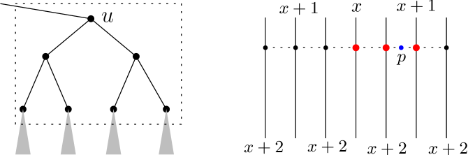
Figure 36: Left: Illustrating the subtree $\mathcal{T}_{u}$, which is in the dotted rectangle (we assume $\log\log n=3$). Right: Illustrating the type-3 Steiner points defined by a point $p$ on $\mathcal{T}_{u}$. The vertical lines are the cut-lines of the nodes in $\mathcal{T}_{u}$ and their level numbers are also shown (we assume that the level number of $u$ is $x$). We assume that $p\in\mathcal{V}(u)$ and $p$ is horizontally visible to all these cut-lines. Then, $p$ defines a type-3 Steiner point on each cut-line. In contrast, only the three big (red) points are type-2 Steiner points defined by $p$ in our original graph $G$

Let $u$ be a node at the highest level of the $i$-th super level of $\mathcal{T}$. Let $\mathcal{T}_{u}$ be the sub-tree of $\mathcal{T}$ rooted at $u$ excluding the nodes outside the $i$-th level (thus $\mathcal{T}_{u}$ has at most $\log n-1$ nodes); e.g., see Fig 36. Recall that $u$ is associated with a subset $\mathcal{V}(u)$ of polygon vertices and each vertex $v\in\mathcal{T}_{u}$ is associated with a cut-line $l(v)$. For each point $p\in\mathcal{V}(u)$ and each vertex $v\in\mathcal{T}_{u}$, if $p$ is horizontally visible to $l(v)$, then $p$ defines a type-3 Steiner point on $l(v)$. In this way, $p$ defines $O(\log n)$ type-3 Steiner points on the cut-lines of $\mathcal{T}_{u}$ (in contrast, $p$ defines only $O(\log\log n)$ type-2 Steiner points on the cut-lines of $\mathcal{T}_{u}$ in our original graph $G$); e.g., see Fig 36. Hence, each polygon vertex $p$ defines a total of $O(\log^{2}n/\log\log n)$ type-3 Steiner points since $\mathcal{T}$ has $O(\log n/\log\log n)$ super-levels. The total number of type-3 Steiner points on all cut-lines is $O(n\log^{2}n/\log\log n)$. Note that each type-2 Steiner point in our original graph $G$ becomes a type-3 Steiner point. For convenience of discussion, those type-3 Steiner points of $G_{1}$ that are originally type-2 Steiner points of $G$ are also called type-2 Steiner points of $G_{1}$.

Type-1 Steiner points are defined in the same way as before, so their number is still $O(n)$. We still use $\mathcal{V}_{1}$ to denote the set of all type-1 Steiner points and all polygon vertices. We use $\mathcal{V}_{2}$ to denote the set of all type-2 Steiner points of $G_{1}$.

The edges of $G_{1}$ are defined with respect to all Steiner points in the same way as $G$. We omit the details. In summary, $G_{1}$ has $O(n\log^{2}n/\log\log n)$ vertices and edges. $G_{1}$ can be computed in $O(n\log^{3}n/\log\log n)$ time (e.g., by using the similar algorithm as in the proof of Lemma 1 in [6]). Note that the original graph $G$ is a sub-graph of $G_{1}$ in that every vertex of $G$ is also a vertex of $G_{1}$ and every path of $G$ corresponds to a path in $G_{1}$ with the same length.

Consider a query point $t$. The gateway set $V^{1}_{g}(t,G_{1})$ is defined in the same way as before, and thus its size is $O(1)$. Thanks to more Steiner points, the size of $V^{2}_{g}(t,G_{1})$ can now be reduced to $O(\log n/\log\log n)$. Specifically, $V^{2}_{g}(t,G_{1})$ is defined as follows (similar to that in [6]).

As in [6], we first define the relevant projection cut-lines of $t$. We only discuss the right side of $t$, and the left side is symmetric. Recall that $t$ has at most one projection cut-line in each level of $\mathcal{T}$. Among all projection cut-lines that are in the same super-level, the one closest to $t$ is called a relevant projection cut-line of $t$. Since there are $O(\log n/\log\log n)$ super-levels and each super-level has at most one relevant projection cut-line to the right of $t$, $t$ has $O(\log n/\log\log n)$ relevant projection cut-lines. For each such cut-line $l$, the Steiner point (if any) immediately above (resp., below) the horizontal projection $t^{\prime}$ of $t$ on $l$ is included in $V_{g}^{2}(t,G_{1})$ if it is visible to $t^{\prime}$. Thus, $|V_{g}^{2}(t,G_{1})|=O(\log n/\log\log n)$.

By Lemma 18, if $|V_{g}^{2}(t,G_{1})|=O(\log n/\log\log n)$, the query time becomes $O(\log n)$ as long as $|V_{g}^{2}(s,G_{1})|=O(\log n)$. This implies that for $s$, we can simply use its original gateway set on type-2 Steiner points, i.e., we define $V_{g}^{2}(s,G_{1})$ in the same way as before with respect to only the type-2 Steiner points of $G_{1}$ (thus $V_{g}^{2}(s,G_{1})=V_{g}^{2}(s,G)$). As will be clear later, this will help save time and space in the preprocessing. We also define $V_{g}^{1}(s,G_{1})$ in the same way as before.

Lemma 16

For any two query points $s$ and $t$, if there does not exist a trivial shortest $s$-$t$ path, then there is a shortest $s$-$t$ path containing a gateway of $s$ and a gateway of $t$.

Proof

Suppose there does not exist a trivial shortest $s$-$t$ path. Then, there is a shortest $s$-$t$ path that contains a polygon vertex. Therefore, to prove the lemma, it is sufficient to show the following: For any polygon vertex $p$, there exists a shortest path from $s$ (resp., $t$) to $p$ that contains a gateway of $s$ (resp., $t$). For the case of $s$, since its gateway set is the same as before in the graph $G$, this has been proved in [7]. For the case of $t$, we can follow the similar analysis as in [6] (i.e., the proof of Lemma 2) because our way of defining $V_{g}^{2}(t,G_{1})$ is similar in spirit to theirs (the only difference is that the size of the gateway set in [6] is $O(\sqrt{\log n})$, which is due to that each super-level of $\mathcal{T}$ in [6] consists of $\sqrt{\log n}$ levels). We omit the details. ∎

Lemma 17

With $O(n\log^{3}n/\log\log n)$ time and $O(n\log^{2}n/\log\log n)$ space preprocessing, we can compute $V_{g}(s,G_{1})$ and $V_{g}(t,G_{1})$ in $O(\log n)$ time for any two query points $s$ and $t$.

Proof

We first discuss the case for $t$. For computing $V_{g}^{1}(t,G_{1})$, as in [6] (see the proof of Lemma 3), it is sufficient to compute the four projection points $t^{d},t^{u},t^{l},t^{r}$ on $\partial\mathcal{P}$, which can be done in $O(\log n)$ time by using the horizontal and vertical decompositions of $\mathcal{P}$. The two decompositions of $\mathcal{P}$ can be computed in $O(n\log n)$ time or $O(n+h\log^{1+\epsilon}h)$ time for any $\epsilon>0$ [3, 4].

For $V_{g}^{2}(t,G_{1})$, we can use the same approach as that in [6] (see the proof of Lemma 3). Since the number of type-3 Steiner points is $O(n\log^{2}n/\log\log n)$, the preprocessing takes $O(n\log^{3}n/\log\log n)$ time and $O(n\log^{2}n/\log\log n)$ space.

For $s$, the set $V_{g}^{1}(s,G_{1})$ can be computed in the same way as $t$. For $V_{g}^{2}(s,G_{1})$, we maintain a data structure for all type-2 Steiner points as in [6] (see the proof of Lemma 3). Since there are $O(n\log n)$ type-2 Steiner points, with $O(n\log^{2}n)$ time and $O(n\log n)$ space preprocessing, we can compute $V_{g}^{2}(s,G_{1})$ in $O(\log n)$ time. ∎

Our preprocessing is similar as before. For each vertex $q$ of $G_{1}$ (which is also considered as a point in $\mathcal{P}$), we compute a shortest path tree $T(q)$ but only for the points in $\mathcal{V}_{1}\cup\mathcal{V}_{2}$ using the algorithm [24, 25]. Since $|\mathcal{V}_{1}\cup\mathcal{V}_{2}|=O(n\log n)$, $T(p)$ has $O(n\log n)$ vertices and can be computed in $O(n\log^{2}n)$ time [24, 25]. We also store the post-order traversal list of $T(p)$. Since $G_{1}$ has $O(n\log^{2}n/\log\log n)$ vertices, the preprocessing takes $O(n^{2}\log^{4}n/\log\log n)$ time and $O(n^{2}\log^{3}n/\log\log n)$ space in total.

Remark.

If we define $V_{g}^{2}(s,G_{1})$ in the same way as $V_{g}^{2}(t,G_{1})$ (i.e., with respect to type-3 Steiner points), then we would need to compute $T(p)$ for all $O(n\log^{2}n/\log\log n)$ type-3 Steiner points in the preprocessing, which would take $O(n^{2}\log^{5}n/(\log\log n)^{2})$ time and $O(n^{2}\log^{4}n/(\log\log n)^{2})$ space.

As a summary, we have the following result.

Lemma 18

With $O(n^{2}\log^{4}n/\log\log n)$ time and $O(n^{2}\log^{3}n/\log\log n)$ space preprocessing, given any two query points $s$ and $t$, we can compute their shortest path length in $O(\log n)$ time and an actual shortest $s$-$t$ path can be output in additional time linear in the number of edges of the path.

Proof

With the new gateway sets $V_{g}(s,G_{1})$ and $V_{g}(t,G_{1})$, applying Lemma 15 directly will lead to the lemma. To guarantee correctness, since we now use new gateway sets $V_{g}^{2}(s,G_{1})$ and $V_{g}^{2}(t,G_{1})$, we need to show that the geometric properties in Section 3 related to these gateways still hold. Specifically, we need to show that the properties of the gateway region $R(s)$ for $s$, i.e., Observations 1 and 2, and the properties of the extended gateway region $R(t)$ for $t$, i.e., Observations 3, 4, 5, 6, and 7, still hold. Indeed, for $R(s)$, its properties obviously hold since $R(s)$ is exactly the same as before (because $V_{g}^{2}(s,G_{1})$ is exactly $V_{g}^{2}(s,G)$). For $R(t)$, its properties also hold. An easy way to see this is that the new $R(t)$ defined based on $V_{g}^{2}(t,G_{1})$ is a subset of the original $R(t)$ defined based on $V_{g}^{2}(t,G)$. ∎

4.1 A Further Improvement

Using the techniques in [6], we can further reduce the complexities of the preprocessing so that they are functions of $h$, in addition to $O(n)$, as shown in the following theorem.

Theorem 4.1

With $O(n+h^{2}\log^{4}h/\log\log h)$ time and $O(n+h^{2}\log^{3}h/\log\log h)$ space preprocessing, given any two query points $s$ and $t$, we can compute their shortest path length in $O(\log n)$ time and an actual shortest $s$-$t$ path can be output in additional time linear in the number of edges of the path.

The main idea is to follow the algorithmic scheme in [6] (i.e., the one in Section 4), by replacing the “enhanced” graph $G_{E}$ with our graph $G_{1}$ and replacing their query algorithm with our new query algorithm. A major difference is that since our query algorithm needs to determine the relative positions of two shortest paths, we will also need to compute (planar) shortest path trees using the algorithms in [8] (we cannot use the shortest path trees in $G_{1}$ because they may not be planar). We only sketch the main idea below, following the notation in [6].

The algorithm in [6] uses an extended corridor structure to decompose $\mathcal{P}$ into an ocean $\mathcal{M}$, and $O(n)$ bays and canals. While $\mathcal{M}$ is multiply-connected, each bay/canal is a simple polygon. Each bay has a gate which is a common edge shared by the bay and $\mathcal{M}$. Each canal has two gates.

A graph $G_{E}(\mathcal{M})$ is built on $\mathcal{M}$ with respect to $O(h)$ special points on the boundary of $\mathcal{M}$. The graph has $O(h\sqrt{\log h}2^{\sqrt{\log h}})$ vertices and edges. Using the graph, with $O(n+h^{2}\log^{2}h4^{\sqrt{\log h}})$ time and $O(n+h^{2}\log h4^{\sqrt{\log h}})$ space preprocessing, if $s$ and $t$ are both in $\mathcal{M}$, a shortest $s$-$t$ path can be computed in $O(\log n)$ time.

For our purpose, we replace the graph $G_{E}(\mathcal{M})$ by our graph $G_{1}(\mathcal{M})$, which is built with respect to the above mentioned $O(h)$ special points on the boundary of $\mathcal{M}$ in the same way as the graph $G_{1}$ with respect to the obstacle vertices of $\mathcal{P}$. Thus, the graph $G_{1}(\mathcal{M})$ has $O(h\log^{2}h/\log\log h)$ vertices and edges. We define the sets $\mathcal{V}_{1}(\mathcal{M})$ and $\mathcal{V}_{2}(\mathcal{M})$ accordingly (in the same way as $\mathcal{V}_{1}$ and $\mathcal{V}_{2}$ defined for $G_{1}$), which together have $O(h\log h)$ points. For each vertex $q$ of $G_{1}(\mathcal{M})$, we need to compute a planar shortest path tree $T(q)$ from $q$ to all points of $\mathcal{V}_{1}(\mathcal{M})\cup\mathcal{V}_{2}(\mathcal{M})$. To this end, if we applied the algorithms in [24, 25] as before, then the total preprocessing would take $\Omega(nh)$ time and space. To make the preprocessing complexities linearly depend on $n$, we use an algorithm in [8] instead. Specifically, we can compute a shortest path tree $T^{\prime}(q)$ among all cores of the obstacles of $\mathcal{P}$ (see [8] for the details). Since the size of $\mathcal{V}_{1}(\mathcal{M})\cup\mathcal{V}_{2}(\mathcal{M})$ is $O(h\log h)$, $T^{\prime}(q)$ can be computed in $O(h\log^{2}h)$ time and $O(h\log h)$ space [8]. In particular, each vertex of $T^{\prime}(q)$ is also a vertex of $T(q)$, and the length of a path in $T^{\prime}(q)$ from $q$ to any vertex $p$ is equal to $d(p,q)$. Although an edge of $T^{\prime}(q)$ may not be in $\mathcal{P}$, the paths in $T^{\prime}(q)$ maintain the same topology as those in $T(q)$, i.e., the relative positions of two paths from $q$ to two vertices in $T^{\prime}(q)$ are consistent with those in $T(q)$ (e.g., this can be seen from the proof of Lemma 2 in [8]). Therefore, we can use $T^{\prime}(q)$ to determine the relative positions of two shortest paths in our query algorithm. In this way, with $O(n+h^{2}\log^{4}h/\log\log h)$ time and $O(n+h^{2}\log^{3}h/\log\log h)$ space preprocessing, we can compute the shortest path length $d(s,t)$ in $O(\log n)$ time.

However, we are not able to output a shortest $s$-$t$ path in additional time linear in the number of edges of the path since a path in $T^{\prime}(q)$ may not be in $\mathcal{P}$ (although we can compute a shortest $s$-$t$ path in $O(n)$ additional time, e.g., see the proof of Lemma 2 in [8]). To resolve this issue, we use the following approach. Note that the query algorithm will return a gateway $p$ of $s$ and a gateway $q$ of $t$ so that there is a shortest $s$-$t$ path containing both $p$ and $q$. Our goal is to find a shortest path in $\mathcal{P}$ from $p$ to $q$ (and then by appending $\overline{sp}$ and $\overline{tq}$, we can obtain a shortest $s$-$t$ path). To this end, we will build another graph $G_{2}(\mathcal{M})$ with the following properties: (1) $G_{2}(\mathcal{M})$ has $O(h\log^{2}h/\log\log h)$ vertices and edges, the same as in $G_{1}(\mathcal{M})$ asymptotically; (2) each vertex of $G_{1}(\mathcal{M})$ is also a vertex in $G_{2}(\mathcal{M})$; (3) for any two vertices $u$ and $v$ of $G_{2}(\mathcal{M})$ that are also vertices of $G_{1}(\mathcal{M})$, a shortest path from $u$ to $v$ in $G_{2}(\mathcal{M})$ corresponds to a shortest path in the plane with the same length. We will discuss the definition of $G_{2}(\mathcal{M})$ later in Section 4.1.1.

With $G_{2}(\mathcal{M})$, to find a shortest path from $p$ to $q$, if we compute a shortest path tree $T^{\prime\prime}(p)$ in $G_{2}(\mathcal{M})$ from $p$ to all vertices of $G_{2}(\mathcal{M})$ in the preprocessing, then we can report the path in $T^{\prime\prime}(p)$ from $p$ to $q$ as a shortest path in time linear in the number of edges of the path. Observe that $p$, which is a gateway of $s$, is a point in $\mathcal{V}_{1}(\mathcal{M})\cup\mathcal{V}_{2}(\mathcal{M})$. Correspondingly, in the preprocessing, for each point $v\in\mathcal{V}_{1}(\mathcal{M})\cup\mathcal{V}_{2}(\mathcal{M})$, which is also a vertex of $G_{2}(\mathcal{M})$, we compute a shortest path tree $T^{\prime\prime}(v)$ in $G_{2}(\mathcal{M})$ from $v$ to all vertices of $G_{2}(\mathcal{M})$. Since $|\mathcal{V}_{1}(\mathcal{M})\cup\mathcal{V}_{2}(\mathcal{M})|=O(h\log h)$ and $G_{2}(\mathcal{M})$ has $O(h\log^{2}h/\log\log h)$ vertices and edges, computing all these shortest path trees takes $O(h^{2}\log^{4}h/\log\log h)$ time and $O(h^{2}\log^{3}h/\log\log h)$ space. In addition, as in [6], we need $O(n)$ space to store “corridor paths” and “elementary curves” (see [6] for the details), and these information will also be used to output actual shortest paths.

The above discusses the case where both $s$ and $t$ are in the ocean $\mathcal{M}$. To process the queries for other cases (i.e., at least one of $s$ and $t$ is not in $\mathcal{M}$), the algorithm in [6] builds an additional graph $G_{E}(g)$ of similar structures for each gate $g$ of a canal or a bay. Then, the graph $G_{E}(\mathcal{M})$ is merged with all these additional graphs $G_{E}(g)$ to obtain a graph $G_{E}(\mathcal{P})$, which has $O(h\sqrt{\log h}2^{\sqrt{\log h}})$ vertices and edges, the same as $G_{E}(\mathcal{M})$ asymptotically. Using $G_{E}(\mathcal{P})$, with $O(n+h^{2}\log^{2}h4^{\sqrt{\log h}})$ time and $O(n+h^{2}\log h4^{\sqrt{\log h}})$ space preprocessing, each query can be answered in $O(\log n)$ time.

For our purpose, we replace each graph $G_{E}(g)$ correspondingly by our graph $G_{1}(g)$ and then obtain a new merged graph $G_{1}(\mathcal{P})$, which has $O(h\log^{2}h/\log\log h)$ vertices and edges. We define $\mathcal{V}_{1}(\mathcal{P})$ and $\mathcal{V}_{2}(\mathcal{P})$ accordingly, which together have $O(h\log h)$ points. Also, for each vertex $p$ of $G_{1}(\mathcal{P})$, we compute a shortest path tree $T^{\prime}(p)$ for all points of $\mathcal{V}_{1}(\mathcal{P})\cup\mathcal{V}_{2}(\mathcal{P})$. This can be done in the same time and space as before in $\mathcal{M}$ asymptotically. The total preprocessing time and space are $O(n+h^{2}\log^{4}h/\log\log h)$ and $O(n+h^{2}\log^{3}h/\log\log h)$, respectively. For any two query points $s$ and $t$, we can apply the query algorithm scheme in [6] along with our new query algorithm in Lemma 15 to compute $d(s,t)$ in $O(\log n)$ time. For reporting an actual shortest $s$-$t$ path, we use the similar approach as above for the ocean case but instead use a graph $G_{2}(\mathcal{P})$, by merging $G_{2}(\mathcal{M})$ with $G_{2}(g)$ for all gates $g$.

In summary, with $O(n+h^{2}\log^{4}h/\log\log h)$ time and $O(n+h^{2}\log^{3}h/\log\log h)$ space preprocessing, given $s$ and $t$, we can compute $d(s,t)$ in $O(\log n)$ time and an actual shortest $s$-$t$ path can be output in additional time linear in the number of edges of the path.

4.1.1 A path-preserving graph

It remains to define the graph $G_{2}(\mathcal{M})$. To do so, we define a graph $G_{2}$ based on $G_{1}$ with respect to all polygon vertices of $\mathcal{P}$ (and thus $G_{2}(\mathcal{M})$ has a similar structure but based on $G_{1}(\mathcal{M})$).

As discussed before, although $G_{1}$ preserves shortest paths among all polygon vertices, it may not preserve shortest paths for all its vertices. Our goal is to modify $G_{1}$ to obtain another graph $G_{2}$, so that each vertex of $G_{1}$ is also in $G_{2}$ and $G_{2}$ preserves shortest paths for all vertices of $G_{1}$. A straightforward way to do so is to build a graph $G^{\prime}$ with respect to all vertices of $G_{1}$ in the same way as we build $G_{1}$ with respect to all polygon vertices. However, since $G_{1}$ has $O(n\log^{2}n/\log\log n)$ vertices, such a graph $G^{\prime}$ would have $O(n\log^{3}n/\log\log n)$ vertices and edges. In contrast, our graph $G_{2}$ only has $O(n\log^{2}n/\log\log n)$ vertices and edges, the same as in $G_{1}$ asymptotically.

Recall that $\mathcal{V}_{1}$ consists of all polygon vertices as well as their projections on $\partial\mathcal{P}$. We define $\mathcal{V}_{3}$ as the set consisting of all type-3 Steiner points of $G_{1}$. Hence, $\mathcal{V}_{2}\subseteq\mathcal{V}_{3}$ and $\mathcal{V}_{1}\cup\mathcal{V}_{3}$ constitutes the vertex set of $G_{1}$.

Suppose we already have the graph $G_{1}$. We change it through the following three steps.

First, for each point $p\in\mathcal{V}_{1}\cup\mathcal{V}_{3}$ and each of $p$’s projection $q$ on $\partial\mathcal{P}$, if $q$ is not in $\mathcal{V}_{1}$, we include $q$ as a new type-1 Steiner point and insert it to $G_{1}$, i.e., make $q$ as a new vertex, add an edge connecting $q$ to $p$ and two edges connecting $q$ to its two adjacent Steiner points on the polygon edge containing $q$. Since $|\mathcal{V}_{1}\cup\mathcal{V}_{3}|=O(n\log^{2}n/\log\log n)$, the above adds $O(n\log^{2}n/\log\log n)$ vertices and edges.

Second, for each point $p\in\mathcal{V}_{1}$ that is not a polygon vertex, we define Steiner points on the cut-lines of $\mathcal{T}$ following the same rule as before for type-2 (not type-3) Steiner points. Specifically, if $p$ is on a cut-line (this happens when the cut-line is through a polygon vertex such that $p$ is a vertical projection of the vertex on $\partial\mathcal{P}$), then the cut-line is already a leaf $u$ of $\mathcal{T}$; otherwise, we add a cut-line through $p$ and insert it as a new leaf $u$ in $\mathcal{T}$ by the $x$-coordinate. In either case, for each node $v$ of $\mathcal{T}$ in the path from $u$ to the root, we let $p$ define a type-2 Steiner point $p^{\prime}$ on $l(v)$ if $p$ is horizontally visible to $l(v)$ and then add two edges connecting $p^{\prime}$ to its two adjacent visible Steiner points on $l(v)$. Since $|\mathcal{V}_{1}|=O(n)$, the above adds $O(n\log n)$ vertices and edges.

Third, for each point $p\in\mathcal{V}_{1}$, let $S(p)$ denote the set of all Steiner points on all cut-lines defined by $p$, including $p$ itself as well as $p^{l}$ and $p^{r}$. Clearly, all points of $S(p)$ are on the segment $\overline{p^{l}p^{r}}$. The current graph has an edge connecting $p$ to each point of $S(p)\setminus\{p\}$, and we remove such edges and instead add an edge to connect each pair of adjacent points of $S(p)$ from left to right. This does not change the number of edges of the graph.

The resulting graph is $G_{2}$, which still has $O(n\log^{2}n/\log\log n)$ vertices and edges. In particular, the following observation is guaranteed by the above first step.

Observation 11

For each point $p\in\mathcal{V}_{1}\cup\mathcal{V}_{3}$, its four projections on $\partial\mathcal{P}$ are all Steiner points (and thus vertices) of $G_{2}$.

We can still construct $G_{2}$ in $O(n\log^{3}n/\log\log n)$ time in a similar way as before. The following lemma shows that $G_{2}$ preserves shortest paths for all points of $\mathcal{V}_{1}\cup\mathcal{V}_{3}$ (i.e., all vertices of $G_{1}$).

Lemma 19

For any two points $p$ and $q$ of $\mathcal{V}_{1}\cup\mathcal{V}_{3}$, a shortest path from $p$ to $q$ in $G_{2}$ is also a shortest path in $\mathcal{P}$.

Proof

Because every polygon vertex is in $\mathcal{V}_{1}\cup\mathcal{V}_{3}$, to prove the lemma, following the proof scheme in [11, 12], it is sufficient to show the following: For any two points $p$ and $q$ in $\mathcal{V}_{1}\cup\mathcal{V}_{3}$ that are visible to each other, $G_{2}$ must have an $xy$-monotone path connecting $p$ and $q$ if the connected component of $R\cap\mathcal{P}$ containing $\overline{pq}$ does not contain any polygon vertex, where $R$ is the rectangle with $\overline{pq}$ as a diagonal. In the following, we assume that $p$ and $q$ are visible to each other and $R^{\prime}$ does not contain any polygon vertex, where $R^{\prime}$ is the connected component of $R\cap\mathcal{P}$ containing $\overline{pq}$. Our goal is to show that $G_{2}$ has an $xy$-monotone path connecting $p$ and $q$. Without loss of generality, we assume that $p$ is to southwest of $q$.

Note that each of $p$ and $q$ is defined by a point in $\mathcal{V}_{1}$, and each of them is contained in a cut-line of $\mathcal{T}$. Let $v_{p}$ and $v_{q}$ be the points in $\mathcal{V}_{1}$ defining $p$ and $q$, respectively. Let $l_{p}$ and $l_{q}$ be the cut-lines containing $p$ and $q$, respectively. Each of $l_{p}$ and $l_{q}$ is stored in a node of the cut-line tree $\mathcal{T}$, and we let $l$ be the cut-line in the lowest common ancestor of the two nodes storing $l_{p}$ and $l_{q}$. Hence, $l$ is between $l_{p}$ and $l_{q}$. Depending on whether the rectangle $R$ is in $\mathcal{P}$, there are two cases.

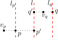
Figure 37: Illustrating the case $R\subseteq\mathcal{P}$.

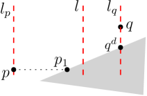
Figure 38: Illustrating the case where $p$ is not horizontally visible to $l$.

If $R\subseteq\mathcal{P}$, then since $v_{p}$ is horizontally visible to $l_{p}$, $v_{p}$ is also horizontally visible to $l$. Since $l$ is an ancestor of $l_{p}$ in $\mathcal{T}$, $v_{p}$ defines a Steiner point $p^{\prime}$ on $l$. For the same reason, $v_{q}$ also defines a Steiner point $q^{\prime}$ on $l$ (e.g., see Fig. 38). Due to the third step for changing $G_{1}$ to obtain $G_{2}$, the path $\overline{pp^{\prime}}\cup\overline{p^{\prime}q^{\prime}}\cup\overline{q^{\prime}q}$ is in $G_{2}$, which is $xy$-monotone.

If $R\not\subseteq\mathcal{P}$, then if both $v_{p}$ and $v_{q}$ are still horizontally visible to $l$, we can use the same analysis as above. Otherwise, without loss of generality, we assume that $p$ is not horizontally visible to $l$. This implies that if we move from $p$ rightwards following the lower edge of $R$, we will encounter a point $p_{1}$ at a polygon edge $e$ before we arrive at $l$ (e.g., see Fig. 38). Note that $p_{1}$ is actually the right projection of $v_{p}$ on $\partial\mathcal{P}$ and thus is a type-1 Steiner point by Observation 11. Since $R^{\prime}$ does not contain any polygon vertex, the downward projection $q^{d}$ of $q$ on $\partial\mathcal{P}$ is on $e$ as well. By Observation 11, $q^{d}$ is a type-1 Steiner point. Note that the slope of $e$ must be positive. Hence, the path $\overline{pp_{1}}\cup\overline{p_{1}q^{d}}\cup\overline{q^{d}q}$, which is in $G_{2}$, is $xy$-monotone.

The lemma is thus proved. ∎

5 Concluding Remarks

In this paper, we present a data structure that can answer two-point $L_{1}$ shortest path queries in a polygonal domain $\mathcal{P}$ in $O(\log n)$ time, and our preprocessing takes nearly quadratic time and space in the number of holes of $\mathcal{P}$ plus linear time and space in the total number of vertices of $\mathcal{P}$. More importantly and interestingly, we propose a divide-and-conquer algorithm that can compute a shortest path in nearly linear time in the number of gateways of $s$ and $t$, improving the previously best and straightforward quadratic time algorithm.

To further improve our result, it might be tempting to see whether the Monge matrix searching techniques [1, 23] can be applied so that the query time becomes linear in the number of gateways of the query points. However, due to those non-ideal situations such as those illustrated in Fig. 4 and Fig. 4, it is not clear to us whether it is possible to do so.

One may wonder whether our divide-and-conquer technique can be applied to the Euclidean case. Indeed, the algorithms in both [5] and [18] for Euclidean two-point shortest path queries are based on the gateway approach (the gateways are called “critical cites” in [18]). More specifically, the method of Chen et al. [5] uses the set $Q_{s}$ of vertices of $\mathcal{P}$ visible to $s$ as the gateway set of $s$, and similarly, the set $Q_{t}$ of vertices of $\mathcal{P}$ visible to $t$ are used as the gateway set of $t$. Without loss of generality, assume $|Q_{s}|\leq|Q_{t}|$. After $Q_{s}$ is computed, for each vertex $v\in Q_{s}$, a shortest path from $s$ to $t$ through $v$ is found by using the shortest path map of $v$ (the map is computed in the preprocessing). In this way, the query time is bounded by $O(\min\{|Q_{s}|,|Q_{t}|\}\cdot\log n)$. By using a tessellation of $\mathcal{P}$, Guo et al. [18] showed that a subset of $Q_{s}$ of size $O(h)$ is sufficient to serve as the gateway set of $s$, and the same holds for $t$. Consequently, the query time can be bounded by $O(h\log n)$. Clearly, the bottleneck of the query time is actually on the number of gateways. To have any hope of achieving a polylogarithmic time query algorithm using gateways, one has to make sure that the number of gateways is polylogarithmic. We are able to achieve this by using path preserving graphs in the $L_{1}$ metric. Such graphs, however, are not applicable to the Euclidean metric. Note that the polylogarithmic time query algorithms by Chiang and Mitchell [10] are based on different techniques (e.g., shortest path map equivalence decompositions) than using gateways. Therefore, for solving the Euclidean two-point shortest path queries, one direction is to see whether it is possible to use only a polylogarithmic number of gateways.

References

- [1] A. Aggarwal, M. Klawe, S. Moran, P. Shor, and R. Wilbur. Geometric applications of a matrix-searching algorithm. Algorithmica, 2:195–208, 1987.
- [2] S.W. Bae and H. Wang. shortest path queries in simple polygons. arXiv:1809.07481, 2018.
- [3] R. Bar-Yehuda and B. Chazelle. Triangulating disjoint Jordan chains. International Journal of Computational Geometry and Applications, 4(4):475–481, 1994.
- [4] B. Chazelle. Triangulating a simple polygon in linear time. Discrete and Computational Geometry, 6:485–524, 1991.
- [5] D.Z. Chen, O. Daescu, and K.S. Klenk. On geometric path query problems. International Journal of Computational Geometry and Applications, 11(6):617–645, 2001.
- [6] D.Z. Chen, R. Inkulu, and H. Wang. Two-point shortest path queries in the plane. Journal of Computational Geometry, 1:473–519, 2016.
- [7] D.Z. Chen, K.S. Klenk, and H.-Y.T. Tu. Shortest path queries among weighted obstacles in the rectilinear plane. SIAM Journal on Computing, 29(4):1223–1246, 2000.
- [8] D.Z. Chen and H. Wang. Computing shortest paths among polygonal obstacles in the plane. Algorithmica, 2019. https://doi.org/10.1007/s00453-018-00540-x.
- [9] D.Z. Chen and J. Xu. Shortest path queries in planar graphs. In Proceedings of the 32nd Annual ACM Symposium on Theory of Computing (STOC), pages 469–478, 2000.
- [10] Y.-J. Chiang and J.S.B. Mitchell. Two-point Euclidean shortest path queries in the plane. In Proceedings of the Annual ACM-SIAM Symposium on Discrete Algorithms (SODA), pages 215–224, 1999.
- [11] K. Clarkson, S. Kapoor, and P. Vaidya. Rectilinear shortest paths through polygonal obstacles in time. In Proceedings of the 3rd Annual Symposium on Computational Geometry (SoCG), pages 251–257, 1987.
- [12] K. Clarkson, S. Kapoor, and P. Vaidya. Rectilinear shortest paths through polygonal obstacles in time. Manuscript, 1988.
- [13] H.N. Djidjev. Efficient algorithms for shortest path queries in planar digraphs. In Proceedings of the 22nd International Workshop on Graph-Theoretic Concepts in Computer Science, pages 151–165, 1996.
- [14] H.A. ElGindy and P. Mitra. Orthogonal shortest route queries among axis parallel rectangular obstacles. International Journal of Computational Geometry and Application, 4:3–24, 1994.
- [15] J. Fakcharoenphol and S. Rao. Planar graphs, negative weight edges, shortest paths, and near linear time. Journal of Computer and System Sciences, 72:868–889, 2006.
- [16] P. Gawrychowski, S. Mozes, O. Weimann, and C. Wulff-Nilsen. Better tradeoffs for exact distance oracles in planar graphs. In Proceedings of the 29rd Annual Symposium on Discrete Algorithms (SODA), pages 515–529, 2018.
- [17] L.J. Guibas and J. Hershberger. Optimal shortest path queries in a simple polygon. Journal of Computer and System Sciences, 39(2):126–152, 1989.
- [18] H. Guo, A. Maheshwari, and J.-R. Sack. Shortest path queries in polygonal domains. In Proceedings of the 4th International Conference on Algorithmic Aspects in Information and Management (AAIM), pages 200–211, 2008.
- [19] J. Hershberger. A new data structure for shortest path queries in a simple polygon. Information Processing Letters, 38(5):231–235, 1991.
- [20] J. Hershberger and J. Snoeyink. Computing minimum length paths of a given homotopy class. Computational Geometry: Theory and Applications, 4(2):63–97, 1994.
- [21] J. Hershberger and S. Suri. An optimal algorithm for Euclidean shortest paths in the plane. SIAM Journal on Computing, 28(6):2215–2256, 1999.
- [22] R. Inkulu and S. Kapoor. Planar rectilinear shortest path computation using corridors. Computational Geometry: Theory and Applications, 42(9):873–884, 2009.
- [23] M.M. Klawe and D.J. Kleitman. An almost linear time algorithm for generalized matrix searching. SIAM Journal on Discrete Mathematics, 3:81–97, 1990.
- [24] J.S.B. Mitchell. An optimal algorithm for shortest rectilinear paths among obstacles. Abstracts of the 1st Canadian Conference on Computational Geometry, 1989.
- [25] J.S.B. Mitchell. shortest paths among polygonal obstacles in the plane. Algorithmica, 8(1):55–88, 1992.
- [26] J.S.B. Mitchell. Shortest paths among obstacles in the plane. International Journal of Computational Geometry and Applications, 6(3):309–332, 1996.
- [27] S. Mozes and C. Sommer. Exact distance oracles for planar graphs. In Proceedings of the 23rd Annual Symposium on Discrete Algorithms (SODA), pages 209–222, 2012.