Multivariate extensions of isotonic regression and total variation denoising via entire monotonicity and Hardy-Krause variation

Abstract

We consider the problem of nonparametric regression when the covariate is $d$-dimensional, where $d\geq 1$. In this paper we introduce and study two nonparametric least squares estimators (LSEs) in this setting — the entirely monotonic LSE and the constrained Hardy-Krause variation LSE. We show that these two LSEs are natural generalizations of univariate isotonic regression and univariate total variation denoising, respectively, to multiple dimensions. We discuss the characterization and computation of these two LSEs obtained from $n$ data points. We provide a detailed study of their risk properties under the squared error loss and fixed uniform lattice design. We show that the finite sample risk of these LSEs is always bounded from above by $n^{-2/3}$ modulo logarithmic factors depending on $d$; thus these nonparametric LSEs avoid the curse of dimensionality to some extent. We also prove nearly matching minimax lower bounds. Further, we illustrate that these LSEs are particularly useful in fitting rectangular piecewise constant functions. Specifically, we show that the risk of the entirely monotonic LSE is almost parametric (at most $1/n$ up to logarithmic factors) when the true function is well-approximable by a rectangular piecewise constant entirely monotone function with not too many constant pieces. A similar result is also shown to hold for the constrained Hardy-Krause variation LSE for a simple subclass of rectangular piecewise constant functions. We believe that the proposed LSEs yield a novel approach to estimating multivariate functions using convex optimization that avoid the curse of dimensionality to some extent.

and

t1Supported by a NSF Graduate Research Fellowship t2Supported by NSF CAREER Grant DMS-1654589 t3Supported by NSF Grants DMS-1712822 and AST-1614743

1 Introduction

Consider the problem of nonparametric regression where the goal is to estimate an unknown regression function $f^{*}:[0,1]^{d}\to\mathbb{R}$ ($d\geq 1$) from noisy observations at fixed design points $\boldsymbol{\mathbf{x}}_{1},\ldots,\boldsymbol{\mathbf{x}}_{n}\in[0,1]^{d}$. Specifically, we observe responses $y_{1},\ldots,y_{n}$ drawn according to the model

$$\qquad y_{i}=f^{*}(\boldsymbol{\mathbf{x}}_{i})+\xi_{i},\qquad\text{where $\;\;\xi_{i}\overset{\text{i.i.d.}}{\sim}\mathcal{N}(0,\sigma^{2})\quad$ for $i=1,\ldots,n$},$$ (1)

$\sigma^{2}>0$ is unknown, and the purpose is to nonparametrically estimate $f^{*}$ known to belong to a prespecified function class. In the univariate ($d=1$) case, two such important function classes are: (i) the class of monotone nondecreasing functions in which case $f^{*}$ is usually estimated by the isotonic least squares estimator (LSE) (see e.g., Robertson et al. [59], Groeneboom and Jongbloed [34], Barlow et al. [5], Brunk [11], Ayer et al. [4]); and (ii) the class of functions whose total variation is bounded by a specific constant in which case it is natural to estimate $f^{*}$ by total variation denoising (see e.g., Rudin et al. [60], Mammen and van de Geer [49], Chambolle et al. [13], Condat [20]). Both these estimators — isotonic regression and total variation denoising — have a long history and are very well-studied. For example, it is known that both these estimators produce piecewise constant fits and have finite sample risk (under the squared error loss) bounded from above by a constant multiple of $n^{-2/3}$ (see e.g., Meyer and Woodroofe [51], Zhang [79], Mammen and van de Geer [49]). Moreover, it is well-known that both these estimators are especially useful in fitting piecewise constant functions where their risk is almost parametric (at most $1/n$ up to logarithmic factors); see e.g., Guntuboyina and Sen [38], Dalalyan et al. [22], and Guntuboyina et al. [37] and the references therein.

In this paper, we try to answer the following question: “What is a natural generalization of univariate isotonic regression and univariate total variation denoising to multiple dimensions?” To answer this question we introduce and study two (constrained) LSEs for estimating $f^{*}:[0,1]^{d}\to\mathbb{R}$ where $d\geq 1$. We show that both these LSEs yield rectangular piecewise constant fits and have finite sample risk that is bounded from above by $n^{-2/3}$ (modulo logarithmic factors depending on $d$), thereby avoiding the curse of dimensionality to some extent. Further, we study the characterization and computation of these two estimators: the LSEs are obtained as solutions to convex optimization problems — in fact, quadratic programs with linear constraints — and are thus easily computable. Moreover, as in the case $d=1$, we illustrate that these LSEs are particularly useful in fitting rectangular piecewise constant functions and can have almost parametric risk (up to logarithmic factors). These results are directly analogous to the univariate results mentioned in the previous paragraph and thus justify our claim that our proposed estimators are natural multivariate generalizations of univariate isotonic regression and univariate total variation denoising.

Our first estimator is the LSE over $\mathcal{F}_{\textup{EM}}^{d}$, the class of entirely monotone functions on $[0,1]^{d}$:

$$\widehat{f}_{\textup{EM}}\in\operatorname*{\arg\!\min}_{f\in\mathcal{F}_{\textup{EM}}^{d}}\frac{1}{n}\sum_{i=1}^{n}(y_{i}-f(\boldsymbol{\mathbf{x}}_{i}))^{2}.$$ (2)

The class $\mathcal{F}_{\textup{EM}}^{d}$ of entirely monotone functions is formally defined in Section 2. Entire monotonicity is an existing generalization in multivariate analysis of the univariate notion of monotonicity (see e.g., [1, 45, 77, 42]). Indeed, in the univariate case when $d=1$, the class $\mathcal{F}_{\textup{EM}}^{1}$ is precisely the class of nondecreasing functions on $[0,1]$ and thus, for $d=1$, the estimator (2) reduces to the usual isotonic LSE. For $d=2$, the class $\mathcal{F}_{\textup{EM}}^{2}$ consists of all functions $f:[0,1]^{2}\rightarrow\mathbb{R}$ which satisfy both $f(a_{1},a_{2})\leq f(b_{1},b_{2})$ and

$$f(b_{1},b_{2})-f(a_{1},b_{2})-f(b_{1},a_{2})+f(a_{1},a_{2})\geq 0,$$ (3)

for every $0\leq a_{1}\leq b_{1}\leq 1$ and $0\leq a_{2}\leq b_{2}\leq 1$. The formal definition of $\mathcal{F}_{\textup{EM}}^{d}$ for general $d\geq 1$ is given in Section 2. We remark that in general, entire monotonicity is different from the usual notion of monotonicity in classical multivariate isotonic regression [59]; see 2.1 for a connection between these two notions. We also remark that $\mathcal{F}_{\textup{EM}}^{d}$ is closed under translation and nonnegative scaling; that is, if $f\in\mathcal{F}_{\textup{EM}}^{d}$, then $af+b\in\mathcal{F}_{\textup{EM}}^{d}$ for any $a\geq 0$ and $b\in\mathbb{R}$. Additionally, the collection of right-continuous functions in $\mathcal{F}_{\textup{EM}}^{d}$ is precisely the collection of cumulative distribution functions of nonnegative measures on $[0,1]^{d}$ (see 2.2).

Our terminology of entire monotonicity is taken from Young and Young [77]. As a word of caution, we note that some authors (e.g., Aistleitner and Dick [1]) use the term “completely monotone” in place of “entirely monotone.” We use the latter terminology because “completely monotone” has been used in the literature for other notions (see e.g., [75, 30, 28]) which are unrelated to our definition of entire monotonicity. Entire monotonicity has also been referred by other names in the literature (for example, it has been referred to as “quasi-monotone” in Hobson [42]).

The second main estimator that we study in this paper involves $V_{\textup{HK}\boldsymbol{\mathbf{0}}}(\cdot)$, the variation in the sense of Hardy and Krause (anchored at $\boldsymbol{\mathbf{0}}$), which we shorten to Hardy-Krause variation or HK$\boldsymbol{\mathbf{0}}$ variation. The HK$\boldsymbol{\mathbf{0}}$ variation of a univariate function $f:[0,1]\to\mathbb{R}$ is simply the total variation of the function, i.e.,

$$V_{\textup{HK}\boldsymbol{\mathbf{0}}}(f)=\sup_{0=x_{0}<x_{1}<\dots<x_{k}=1}\sum_{i=0}^{k-1}|f(x_{i+1})-f(x_{i})|,$$ (4)

where the supremum is over all $k\geq 1$ and all partitions $0=x_{0}<x_{1}<\dots<x_{k}=1$ of $[0,1]$. Thus HK$\boldsymbol{\mathbf{0}}$ variation is a generalization of one-dimensional total variation to multiple dimensions. For $d=2$, HK$\boldsymbol{\mathbf{0}}$ variation is defined in the following way: for $f:[0,1]^{2}\to\mathbb{R}$,

$$\begin{split}V_{\textup{HK}\boldsymbol{\mathbf{0}}}(f)&\coloneqq V_{\textup{HK}\boldsymbol{\mathbf{0}}}(x\mapsto f(x,0))+V_{\textup{HK}\boldsymbol{\mathbf{0}}}(x\mapsto f(0,x))\\ &\phantom{{}\coloneqq}\quad+\sup\sum_{0\leq l_{1}<k_{1},0\leq l_{2}<k_{2}}\left|f(x_{l_{1}+1}^{(1)},x_{l_{2}+1}^{(2)})-f(x_{l_{1}}^{(1)},x_{l_{2}+1}^{(2)})\right.\\ &\phantom{{}\coloneqq\quad+\sup\sum_{0\leq l_{1}<k_{1},0\leq l_{2}<k_{2}}{}}\quad\left.-f(x_{l_{1}+1}^{(1)},x_{l_{2}}^{(2)})+f(x_{l_{1}}^{(1)},x_{l_{2}}^{(2)})\right|\end{split}$$ (5)

where the first two terms in the right hand side above are defined via the univariate definition (4) and the supremum in the third term above is over all pairs of partitions $0=x_{0}^{(1)}<x_{1}^{(1)}<\dots<x_{k_{1}}^{(1)}=1$ and $0=x_{0}^{(2)}<x_{1}^{(2)}<\dots<x_{k_{2}}^{(2)}=1$ of $[0,1]$. Note that a special role is played in the first two terms of the right hand side of (5) by the point $(0,0)$ and this is the reason for the phrase “anchored at $\boldsymbol{\mathbf{0}}$”. For smooth functions $f:[0,1]^{2}\rightarrow\mathbb{R}$, it can be shown that

$$V_{\textup{HK}\boldsymbol{\mathbf{0}}}(f)=\int_{0}^{1}\int_{0}^{1}\left|\frac{\partial^{2}f}{\partial x_{1}\partial x_{2}}\right|dx_{1}dx_{2}+\int_{0}^{1}\left|\frac{\partial f(\cdot,0)}{\partial x_{1}}\right|dx_{1}+\int_{0}^{1}\left|\frac{\partial f(0,\cdot)}{\partial x_{2}}\right|dx_{2}$$

and, from the first term in the right hand side above, it is clear that the HK$\boldsymbol{\mathbf{0}}$ variation is related to the $L^{1}$ norm of the mixed derivative. The definition of HK$\boldsymbol{\mathbf{0}}$ variation for general $d\geq 1$ is given in Section 2. HK$\boldsymbol{\mathbf{0}}$ variation is quite different from the usual definition of multivariate total variation (see e.g., Ziemer [81, Chapter 5]) as explained briefly in Section 2.

Functions that are piecewise constant on axis-aligned rectangular pieces (see 2.3) have finite HK$\boldsymbol{\mathbf{0}}$ variation as explained in Section 2. More generally, the collection of right-continuous functions of finite HK$\boldsymbol{\mathbf{0}}$ variation is precisely the same as the collection of cumulative distribution functions of finite signed measures (see 2.5). An example of a function with infinite HK$\boldsymbol{\mathbf{0}}$ variation is the indicator function of an open $d$-dimensional ball contained in $[0,1]^{d}$ (see [57, Sec. 12]).

Our second estimator is the constrained LSE over functions with HK$\boldsymbol{\mathbf{0}}$ variation bounded by some tuning parameter $V>0$:

$$\widehat{f}_{\textup{HK}\boldsymbol{\mathbf{0}},V}\in\operatorname*{\arg\!\min}_{f:V_{\textup{HK}\boldsymbol{\mathbf{0}}}(f)\leq V}\frac{1}{n}\sum_{i=1}^{n}(y_{i}-f(\boldsymbol{\mathbf{x}}_{i}))^{2}.$$ (6)

This estimator is a generalization of total variation denoising to $d\geq 2$ because in the case $d=1$, HK$\boldsymbol{\mathbf{0}}$ variation coincides with total variation and, thus, the above estimator performs univariate total variation denoising, sometimes also called trend filtering of first order [60, 49, 13, 20, 44, 66]. This generalization is different from the usual multivariate total variation denoising as in Rudin et al. [60] (see Section 5 for more discussion on how $\widehat{f}_{\textup{HK}\boldsymbol{\mathbf{0}},V}$ is different from the multivariate total variation regularized estimator). It is also possible to define the HK$\boldsymbol{\mathbf{0}}$ variation estimator in the following penalized form:

$$\widehat{f}_{\textup{HK}\boldsymbol{\mathbf{0}},\lambda}\in\operatorname*{\arg\!\min}_{f}\frac{1}{n}\left\{\sum_{i=1}^{n}(y_{i}-f(\boldsymbol{\mathbf{x}}_{i}))^{2}+\lambda V_{\textup{HK}\boldsymbol{\mathbf{0}}}(f)\right\}$$ (7)

for a tuning parameter $\lambda>0$. In this paper, we shall focus on the constrained form in (6) although analogues of our results for the penalized estimator (7) can also be proved.

Before proceeding further, let us note that entire monotonicity is related to HK$\boldsymbol{\mathbf{0}}$ variation in much the same way as univariate monotonicity is related to univariate total variation. Indeed, for functions in one variable, the following two properties are well-known:

1. Every function $f:[0,1]\rightarrow\mathbb{R}$ of bounded variation can be written as the difference of two monotone functions $f=f_{+}-f_{-}$ and the total variation of $f$ equals the sum of the variations of $f_{+}$ and $f_{-}$.

2. If $f:[0,1]\rightarrow\mathbb{R}$ is nondecreasing, then its total variation on $[0,1]$ is simply $f(1)-f(0)$.

These two facts generalize almost verbatim to entire monotonicity and HK$\boldsymbol{\mathbf{0}}$ variation (see 2.4). Thus, in some sense, entire monotonicity is to Hardy-Krause variation as monotonicity is to total variation.

Although the terminology of “entire monotonicity” does not seem to have been used previously in the statistics literature, entirely monotone functions are closely related to cumulative distribution functions of nonnegative measures which appear routinely in statistics. HK$\boldsymbol{\mathbf{0}}$ variation has appeared previously in statistics in the literature on quasi-Monte Carlo (see e.g., [57, 39]) as well as in the power analysis of certain sequential detection problems (see e.g., [58]). Additionally Benkeser and Van Der Laan [9] (see also [69, 68, 71, 70]) considered the class $\{f:V_{\textup{HK}\boldsymbol{\mathbf{0}}}(f)\leq V\}$ in their “highly adaptive LASSO” estimator and exploited its connections to the LASSO in a setting that is different from our classical nonparametric regression framework. They also used the terminology of “sectional variation norm” to refer to the Hardy-Krause variation (see also [31, Section 2]). An estimator very similar to (6) was proposed by Mammen and van de Geer [49] for $d=2$ when the design points take values in a uniformly spaced grid (this estimator of [49] is described in Section 3.1). Also, Lin [47] proposed an estimator in the context of the Gaussian white noise model that bears some similarities to (6) (this connection is detailed in Section 5).

The goal of this paper is to analyze the properties of the estimators (2) and (6). Here is a description of our main results. Section 3 concerns the computation of these estimators. Note that, as stated, the optimization problems defining our estimators (2) and (6) are convex (albeit infinite-dimensional). We show that, given arbitrary data $(\boldsymbol{\mathbf{x}}_{1},y_{1}),\dots,(\boldsymbol{\mathbf{x}}_{n},y_{n})$, the two estimators (2) and (6) can be computed by solving a nonnegative least squares (NNLS) problem and a LASSO problem respectively, with a suitable design matrix that only depends on the design-points $\boldsymbol{\mathbf{x}}_{1},\dots,\boldsymbol{\mathbf{x}}_{n}$. It is interesting to note that the design matrices in the two finite-dimensional problems for computing (2) and (6) are exactly the same. Our main results in this section (3.1 and 3.3) imply that $\widehat{f}_{\textup{EM}}$ and $\widehat{f}_{\textup{HK}\boldsymbol{\mathbf{0}},V}$ can be taken to be of the form

$$\widehat{f}_{\textup{EM}}=\sum_{j=1}^{p}(\widehat{\beta}_{\textup{EM}})_{j}\cdot\mathbb{I}_{[\boldsymbol{\mathbf{z}}_{j},\boldsymbol{\mathbf{1}}]}~{}~{}\text{ and }~{}~{}\widehat{f}_{\textup{HK}\boldsymbol{\mathbf{0}},V}=\sum_{j=1}^{p}(\widehat{\beta}_{\textup{HK}\boldsymbol{\mathbf{0}},V})_{j}\cdot\mathbb{I}_{[\boldsymbol{\mathbf{z}}_{j},\boldsymbol{\mathbf{1}}]}$$ (8)

for some $\boldsymbol{\mathbf{z}}_{1},\dots,\boldsymbol{\mathbf{z}}_{p}$ that only depend on the design points $\boldsymbol{\mathbf{x}}_{1},\dots,\boldsymbol{\mathbf{x}}_{n}$ and vectors $\boldsymbol{\mathbf{\widehat{\beta}}}_{\textup{EM}}$ and $\boldsymbol{\mathbf{\widehat{\beta}}}_{\textup{HK}\boldsymbol{\mathbf{0}},V}$ in $\mathbb{R}^{p}$ which are obtained by solving the NNLS problem (37) and the LASSO problem (40) respectively. Here $\mathbb{I}_{[\boldsymbol{\mathbf{z}}_{j},\boldsymbol{\mathbf{1}}]}$ denotes the indicator of the rectangle $[\boldsymbol{\mathbf{z}}_{j},\boldsymbol{\mathbf{1}}]$ (defined via (19)). Because NNLS and LASSO typically lead to sparse solutions, the vectors $\boldsymbol{\mathbf{\widehat{\beta}}}_{\textup{EM}}$ and $\boldsymbol{\mathbf{\widehat{\beta}}}_{\textup{HK}\boldsymbol{\mathbf{0}},V}$ will be sparse which clearly implies that $\widehat{f}_{\textup{EM}}$ and $\widehat{f}_{\textup{HK}\boldsymbol{\mathbf{0}},V}$ as given above (8) will be piecewise constant on axis-aligned rectangles. Therefore our estimators give rectangular piecewise constant fits to data and this generalizes the fact that univariate isotonic regression and total variation denoising yield piecewise constant fits. In the case when the design points $\boldsymbol{\mathbf{x}}_{1},\dots,\boldsymbol{\mathbf{x}}_{n}$ form an equally spaced lattice in $[0,1]^{d}$ (see the definition (46) for the precise formulation of this assumption), the points $\boldsymbol{\mathbf{z}}_{1},\dots,\boldsymbol{\mathbf{z}}_{p}$ can simply be taken to be $\boldsymbol{\mathbf{x}}_{1},\dots,\boldsymbol{\mathbf{x}}_{n}$ and, in this case, more explicit expressions can be given for the estimators (see Section 3.1 for details). It should be noted that the lattice design is quite commonly used for theoretical studies in multidimensional nonparametric function estimation (see e.g., [52]) especially in connection with image analysis (see e.g., [13, 21]).

We also investigate the accuracy properties of $\widehat{f}_{\textup{EM}}$ and $\widehat{f}_{\textup{HK}\boldsymbol{\mathbf{0}},V}$ via the study of their risk behavior under the standard fixed design squared error loss function. Specifically, we define the risk of an estimator $\widehat{f}$ by

$$\mathcal{R}(\widehat{f},f^{*})\coloneqq\mathbb{E}\mathcal{L}(\widehat{f},f^{*})\qquad\text{where $\quad\mathcal{L}(\widehat{f},f^{*})\coloneqq\frac{1}{n}\sum_{i=1}^{n}(\widehat{f}(\boldsymbol{\mathbf{x}}_{i})-f^{*}(\boldsymbol{\mathbf{x}}_{i}))^{2}$}.$$ (9)

We prove results on the risk of $\widehat{f}_{\textup{EM}}$ and $\widehat{f}_{\textup{HK}\boldsymbol{\mathbf{0}},V}$ in the case of the aforementioned lattice design. In this setting, our main results are described below.

We analyze the risk of $\widehat{f}_{\textup{EM}}$ under the (well-specified) assumption that $f^{*}\in\mathcal{F}_{\textup{EM}}^{d}$. We prove in Theorem 4.1 that, for $n\geq 1$,

$$\mathcal{R}(\widehat{f}_{\textup{EM}},f^{*})\leq\frac{C(d,\sigma,V^{*})}{n^{2/3}}(\log(en))^{\frac{2d-1}{3}}$$ (10)

where

$$V^{*}:=f^{*}(1,\dots,1)-f^{*}(0,\dots,0)$$ (11)

and $C(d,\sigma,V^{*})$ depends only on $d$, $\sigma$ and $V^{*}$ (see statement of Theorem 4.1 for the explicit form of $C(d,\sigma,V^{*})$). Note that the dimension $d$ appears in (10) only through the logarithmic term which means that we obtain “dimension independent rates” ignoring logarithmic factors. Some intuition for why the constraint of entire monotononicity is able to mitigate the usual curse of dimensionality is provided in Section 5. Other nonparametric estimators exhibiting such dimension independent rates can be found in [6, 47, 19, 53, 62, 74]. In Theorem 4.2, we prove a minimax lower bound which implies that the dependence on $d$ through the logarithmic term in (10) cannot be avoided for any estimator.

We also prove in Theorem 4.4 that $\mathcal{R}(\widehat{f}_{\textup{EM}},f^{*})$ is smaller than the bound given by (10) when $f^{*}\in\mathcal{F}_{\textup{EM}}^{d}$ is rectangular piecewise constant. Loosely speaking, we say that $f:[0,1]^{d}\rightarrow\mathbb{R}$ is rectangular piecewise constant if it is constant on each set in a partition of $[0,1]^{d}$ into axis-aligned rectangles and the smallest cardinality of such a partition shall be denoted by $k(f)$ (see 2.3 for the precise definitions). In Theorem 4.4, we prove that whenever $f^{*}\in\mathcal{F}_{\textup{EM}}^{d}$ is rectangular piecewise constant, we have

$$\mathcal{R}(\widehat{f}_{\textup{EM}},f^{*})\leq C_{d}\sigma^{2}\frac{k(f^{*})}{n}(\log(en))^{\frac{3d}{2}}(\log(e\log(en)))^{\frac{2d-1}{2}}$$ (12)

for a positive constant $C_{d}$ which only depends on $d$. Note that when $k(f^{*})$ is not too large, the right hand side of (12) converges to zero as $n\rightarrow\infty$ at a faster rate compared to the right hand side of (10). Thus rectangular piecewise constant functions which also satisfy the constraint of entire monotonicity are estimated at nearly the parametric rate (ignoring the logarithmic factor) by the LSE $\widehat{f}_{\textup{EM}}$.

Let us now describe our results for the other estimator $\widehat{f}_{\textup{HK}\boldsymbol{\mathbf{0}},V}$. In Theorem 4.5 we prove that when $V_{\textup{HK}\boldsymbol{\mathbf{0}}}(f^{*})\leq V$ (note that $V$ is the tuning parameter in the definition of $\widehat{f}_{\textup{HK}\boldsymbol{\mathbf{0}},V}$), then

$$\mathcal{R}(\widehat{f}_{\textup{HK}\boldsymbol{\mathbf{0}},V},f^{*})\leq\frac{C(d,\sigma,V)}{n^{2/3}}(\log(en))^{\frac{2d-1}{3}}.$$ (13)

Note that the right sides of the bounds (13) and (10) are the same and thus the estimator $\widehat{f}_{\textup{HK}\boldsymbol{\mathbf{0}},V}$ also achieves dimension independent rates (ignoring logarithmic factors) (see Section 5 for an explanation of this phenomenon). We also prove a minimax lower bound in Theorem 4.6 which implies that the dependence on $d$ in the logarithmic term in (13) cannot be completely removed for any estimator.

In univariate total variation denoising, it is known that one obtains faster rates than given by the bound (13) when $f^{*}:[0,1]\rightarrow\mathbb{R}$ is piecewise constant with not too many pieces. Indeed if $f^{*}$ is piecewise constant for $d=1$ with $k(f^{*})$ pieces, then it has been proved that

$$\mathcal{R}(\widehat{f}_{\textup{HK}\boldsymbol{\mathbf{0}},V},f^{*})\leq C(c)\sigma^{2}\frac{k(f^{*})}{n}\log(en)$$ (14)

provided $V=V_{\textup{HK}\boldsymbol{\mathbf{0}}}(f^{*})$ and $f^{*}$ satisfies a minimum length condition in that each constant piece has length at least $c/k(f^{*})$ (the multiplicative term $C(c)$ in (14) only depends on this $c$ appearing in the minimum length condition). A proof of this result can be found in [37, Corollary 2.3] and, for other similar results, see [46, 22, 54, 80]. In light of this univariate result, it is plausible to expect a bound similar to (12) for $\widehat{f}_{\textup{HK}\boldsymbol{\mathbf{0}},V}$ when $f^{*}$ is an axis-aligned rectangular piecewise constant function provided that the tuning parameter $V$ is taken to be equal to $V_{\textup{HK}\boldsymbol{\mathbf{0}}}(f^{*})$ and provided that $f^{*}$ satisfies a minimum length condition. We prove such a result for a class of simple rectangular piecewise constant functions $f^{*}:[0,1]^{d}\rightarrow\mathbb{R}$ of the form

$$f^{*}(\cdot)=a_{1}\mathbb{I}_{[\boldsymbol{\mathbf{x}}^{*},\boldsymbol{\mathbf{1}}]}(\cdot)+a_{0}$$ (15)

for some $a_{1},a_{0}\in\mathbb{R}$ and $\boldsymbol{\mathbf{x}}^{*}\in[0,1]^{d}$ (here $\mathbb{I}$ stands for the indicator function). It is easy to see that (15) represents a rectangular piecewise constant function with $k(f^{*})\leq 2^{d}$. In Theorem 4.7, we prove that when $f^{*}$ is of the above form (15), then

$$\mathcal{R}(\widehat{f}_{\textup{HK}\boldsymbol{\mathbf{0}},V},f^{*})\leq C(c,d)\frac{\sigma^{2}}{n}(\log(en))^{\frac{3d}{2}}(\log(e\log(en)))^{\frac{2d-1}{2}}$$ (16)

provided the tuning parameter $V$ equals $V_{\textup{HK}\boldsymbol{\mathbf{0}}}(f^{*})$ and $\boldsymbol{\mathbf{x}}^{*}\in[0,1]^{d}$ satisfies a minimum size condition (72). This latter condition, which is analogous to the minimum length condition in the univariate case, involves a positive constant $c$ and the constant $C(c,d)$ appearing in (16) only depends on $c$ and the dimension $d$. In the specific case when $d=2$, the minimum length condition (72) can be weakened, as discussed in Section 6.

We are unable to prove versions of (16) for more general rectangular piecewise constant functions. However, some results in that direction have been proved in a very recent paper by Ortelli and van de Geer [54]. Their results are of a different flavor as they work with a similar but different estimator and a smaller loss function. Their proof techniques are also completely different from ours.

The rest of the paper is organized as follows. The notions of entire monotonicity and Hardy-Krause variation are formally defined for arbitrary $d\geq 1$ in Section 2 where we also collect some of their relevant properties. In Section 3, we discuss the computational aspects for solving the optimization problems in (2) and (6). The risk results for $\widehat{f}_{\textup{EM}}$ are given in Section 4.1 while the risk bounds for $\widehat{f}_{\textup{HK}\boldsymbol{\mathbf{0}},V}$ are in Section 4.2. We discuss the connections of our contributions with other related work in Section 5. The proofs for our risk results are given in Section 8 while the proofs of the results in Section 2 and Section 3 are given in Section 9. Additional technical results used in the proofs of Section 8 are proved in Section 10. Section 6 contains another risk bound for $\widehat{f}_{\textup{HK}\boldsymbol{\mathbf{0}},V}$, and Section 7 contains the results of some simulations that includes depictions of the two estimators, as well as an application to estimation in the bivariate current status model.

2 Entire monotonicity and Hardy-Krause variation

The aim of this section is to provide formal definitions of entire monotonicity and HK$\boldsymbol{\mathbf{0}}$ variation for the convenience of the reader. We roughly follow the notation of Aistleitner and Dick [1] and Owen [57].

Let us first introduce some basic notation that will be used throughout the paper. We let $\boldsymbol{\mathbf{0}}=(0,\dots,0)$ and $\boldsymbol{\mathbf{1}}=(1,\dots,1)$. Given an integer $m$, we take $[m]\coloneqq\{1,\ldots,m\}$. For two points $\boldsymbol{\mathbf{a}}=(a_{1},\dots,a_{d})$ and $\boldsymbol{\mathbf{b}}=(b_{1},\dots,b_{d})\in[0,1]^{d}$, we write

$$\boldsymbol{\mathbf{a}}\prec\boldsymbol{\mathbf{b}}~{}~{}\text{ if and only if }~{}~{}a_{j}<b_{j}\text{ for every }j=1,\dots,d$$ (17)

and

$$\boldsymbol{\mathbf{a}}\preceq\boldsymbol{\mathbf{b}}~{}~{}\text{ if and only if }~{}~{}a_{j}\leq b_{j}\text{ for every }j=1,\dots,d.$$ (18)

When $\boldsymbol{\mathbf{a}}\preceq\boldsymbol{\mathbf{b}}$, we write

$$[\boldsymbol{\mathbf{a}},\boldsymbol{\mathbf{b}}] \coloneqq\left\{\boldsymbol{\mathbf{x}}:\boldsymbol{\mathbf{a}}\preceq\boldsymbol{\mathbf{x}}\preceq\boldsymbol{\mathbf{b}}\right\}\coloneqq\prod_{j=1}^{d}[a_{j},b_{j}],$$ (19)

$$[\boldsymbol{\mathbf{a}},\boldsymbol{\mathbf{b}}) \coloneqq\left\{\boldsymbol{\mathbf{x}}:\boldsymbol{\mathbf{a}}\preceq\boldsymbol{\mathbf{x}}\prec\boldsymbol{\mathbf{b}}\right\}\coloneqq\prod_{j=1}^{d}[a_{j},b_{j}).$$ (20)

Note that $[\boldsymbol{\mathbf{a}},\boldsymbol{\mathbf{b}}]$ is a closed axis-aligned rectangle and it has nonempty interior when $\boldsymbol{\mathbf{a}}\prec\boldsymbol{\mathbf{b}}$.

Given a function $f:[0,1]^{d}\rightarrow\mathbb{R}$ and two distinct points $\boldsymbol{\mathbf{a}}=(a_{1},\dots,a_{d}),\boldsymbol{\mathbf{b}}=(b_{1},\dots,b_{d})\in[0,1]^{d}$ with $\boldsymbol{\mathbf{a}}\preceq\boldsymbol{\mathbf{b}}$, we define the quasi-volume $\Delta(f;[\boldsymbol{\mathbf{a}},\boldsymbol{\mathbf{b}}])$ by

$$\sum_{j_{1}=0}^{J_{1}}\cdots\sum_{j_{d}=0}^{J_{d}}(-1)^{j_{1}+\dots+j_{d}}f\left(b_{1}+j_{1}(a_{1}-b_{1}),\ldots,b_{d}+j_{d}(a_{d}-b_{d})\right),$$ (21)

where $J_{i}\coloneqq\mathbb{I}\{a_{i}\neq b_{i}\}$ for each $i$. For example, when $d=2$, it is easy to see that $\Delta(f;[\boldsymbol{\mathbf{a}},\boldsymbol{\mathbf{b}}])$ equals

$$f(b_{1},b_{2})-f(b_{1},a_{2})-f(a_{1},b_{2})+f(a_{1},a_{2})~{}~{}\text{if }\boldsymbol{\mathbf{a}}\prec\boldsymbol{\mathbf{b}}$$ (22)

$$f(b_{1},b_{2})-f(b_{1},a_{2})~{}~{}\text{if }a_{1}=b_{1}\text{ and }a_{2}<b_{2}$$

$$f(b_{1},b_{2})-f(a_{1},b_{2})~{}~{}\text{if }a_{2}=b_{2}\text{ and }a_{1}<b_{1}.$$

We are now ready to define entire monotonicity.

Definition 2.1 (Entire monotonicity).

We say that a function $f:[0,1]^{d}\rightarrow\mathbb{R}$ is entirely monotone if

$$\Delta(f;[\boldsymbol{\mathbf{a}},\boldsymbol{\mathbf{b}}])\geq 0\qquad\text{for every $\boldsymbol{\mathbf{a}}\neq\boldsymbol{\mathbf{b}}\in[0,1]^{d}$ with $\boldsymbol{\mathbf{a}}\preceq\boldsymbol{\mathbf{b}}$}.$$ (23)

In words, for a entirely monotone function $f$, every quasi-volume $\Delta(f;[\boldsymbol{\mathbf{a}},\boldsymbol{\mathbf{b}}])$ is nonnegative. The class of such functions will be denoted by $\mathcal{F}_{\textup{EM}}^{d}$. By (22), note that entire monotonicity is equivalent to (3) for $d=2$.

A more common generalization of monotonicity to multiple dimensions is the class $\mathcal{F}_{\textup{M}}^{d}$ consisting of all functions $f:[0,1]^{d}\rightarrow\mathbb{R}$ satisfying

$$f(a_{1},\dots,a_{d})\leq f(b_{1},\dots,b_{d}),\qquad\text{for $0\leq a_{i}\leq b_{i}\leq 1,\quad i=1,\dots,d$}.$$ (24)

As the following result shows (see Section 9.1 for a proof), $\mathcal{F}_{\textup{EM}}^{d}$ is a strict subset of $\mathcal{F}_{\textup{M}}^{d}$ when $d\geq 2$ (e.g., when $d=2$, functions in $\mathcal{F}_{\textup{EM}}^{d}$ need to additionally satisfy the second constraint in (3)) and thus the estimator (2) is distinct from the LSE over $\mathcal{F}_{\textup{M}}^{d}$ for $d\geq 2$. This latter estimator is the classical multivariate isotonic regression estimator [59].

Lemma 2.1.

When $d=1$, entire monotonicity coincides with monotonicity, i.e., $\mathcal{F}_{\textup{EM}}^{1}=\mathcal{F}_{\textup{M}}^{1}$. For $d\geq 2$, we have $\mathcal{F}_{\textup{EM}}^{d}\subsetneq\mathcal{F}_{\textup{M}}^{d}$.

It is well-known that entirely monotone functions are closely related to cumulative distribution functions of nonnegative measures. The following result taken from Aistleitner and Dick [1, Theorem 3] makes this connection precise.

Lemma 2.2 ([1, Theorem 3]).

1. For every nonnegative Borel measure $\nu$ on $[0,1]^{d}$, the function $f(\boldsymbol{\mathbf{x}}):=\nu([\boldsymbol{\mathbf{0}},\boldsymbol{\mathbf{x}}])$ belongs to $\mathcal{F}_{\textup{EM}}^{d}$.

2. If $f\in\mathcal{F}_{\textup{EM}}^{d}$ is right-continuous, then there exists a unique nonnegative Borel measure $\nu$ on $[0,1]^{d}$ such that $f(\boldsymbol{\mathbf{x}})-f(\boldsymbol{\mathbf{0}})=\nu([\boldsymbol{\mathbf{0}},\boldsymbol{\mathbf{x}}])$.

We shall now define the notion of HK$\boldsymbol{\mathbf{0}}$ variation. The HK$\boldsymbol{\mathbf{0}}$ variation is defined through another variation called the Vitali variation. Let us first define the Vitali variation of a function $f:[0,1]^{d}\rightarrow\mathbb{R}$. To do so, we need some notation. By a partition of the univariate interval $[0,1]$, we mean a set of points $0=x_{0}<x_{1}<\dots<x_{k}=1$ for some $k\geq 1$. Given $d$ such univariate partitions:

$$0=x_{0}^{(s)}<x_{1}^{(s)}<\dots<x_{k_{s}}^{(s)}=1,\qquad\quad\mbox{for $s=1,\dots,d$,}$$ (25)

we can define a collection $\mathcal{P}$ of subsets of $[0,1]^{d}$ consisting of all sets of the form $A_{1}\times\dots\times A_{d}$ where for each $1\leq s\leq d$, $A_{s}=[x_{l_{s}}^{(s)},x_{l_{s}+1}^{(s)}]$ for some $0\leq l_{s}\leq k_{s}-1$. Note that each set in $\mathcal{P}$ is an axis-aligned closed rectangle and the cardinality of $\mathcal{P}$ equals $k_{1}\dots k_{d}$. The rectangles in $\mathcal{P}$ are not disjoint but they form a split of $[0,1]^{d}$ in the sense of Owen [57, Definition 3] and we shall refer to $\mathcal{P}$ as the split generated by the $d$ univariate partitions (25).

Definition 2.2 (Vitali variation).

The Vitali variation of a function $f:[0,1]^{d}\rightarrow\mathbb{R}$ is defined as

$$V^{(d)}(f;[0,1]^{d})\coloneqq\sup_{\mathcal{P}}\sum_{A\in\mathcal{P}}|\Delta(f;A)|$$ (26)

where $\Delta(f;A)$ is the quasi-volume defined in (21) and the supremum above is taken over all splits $\mathcal{P}$ that are generated by $d$ univariate partitions in the manner described above.

The following observations about the Vitali variation will be useful for us. Note first that when $d=1$, Vitali variation is simply total variation (4) since the rectangles in this case are intervals. The second fact is that when $f$ is smooth (in the sense that the partial derivatives appearing below exist and are continuous on $[0,1]^{d}$), we have

$$V^{(d)}(f;[0,1]^{d})=\int_{0}^{1}\dots\int_{0}^{1}\left|\frac{\partial^{d}f}{\partial x_{1}\dots\partial x_{d}}\right|dx_{1}\dots dx_{d}.$$ (27)

The third observation is that $V^{(d)}(f;[0,1]^{d})$ can be written out explicitly when $f$ is a rectangular piecewise constant function. In order to state this result, let us formally define the notion of a rectangular piecewise constant function on $[0,1]^{d}$. Given $d$ univariate partitions as in (25), let $\mathcal{P}^{*}$ denote the collection of all sets of the form $A_{1}\times\dots\times A_{d}$ where for each $1\leq s\leq d$, $A_{s}$ is either equal to $[x_{l_{s}}^{(s)},x_{l_{s}+1}^{(s)})$ for some $0\leq l_{s}\leq k_{s}-1$ or the singleton $\{1\}$. Note that, unlike $\mathcal{P}$, the sets in $\mathcal{P}^{*}$ are disjoint and hence $\mathcal{P}^{*}$ forms a partition of $[0,1]^{d}$. We shall refer to $\mathcal{P}^{*}$ as the partition generated by the $d$ univariate partitions (25).

Definition 2.3 (Rectangular piecewise constant function).

We say that $f:[0,1]^{d}\rightarrow\mathbb{R}$ is rectangular piecewise constant if there exists a partition $\mathcal{P}^{*}$ generated by $d$ univariate partitions as described above such that $f$ is constant on each set in $\mathcal{P}^{*}$. We use $\mathfrak{R}^{d}$ to denote the class of all rectangular piecewise constant functions on $[0,1]^{d}$. For $f\in\mathfrak{R}^{d}$, we define $k(f)$ as the smallest value of $k_{1}\dots k_{d}$ for which there exist $d$ univariate partitions of lengths $k_{1},\dots,k_{d}$ such that $f$ is constant on each of the sets in $\mathcal{P}^{*}$ generated by these $d$ univariate partitions.

The following lemma (proved in Section 9.2) provides a formula for the Vitali variation of a rectangular piecewise constant function $f$ on $[0,1]^{d}$. Note that this lemma implies, in particular, that the Vitali variation of every rectangular piecewise constant function is finite.

Lemma 2.3.

Suppose $f$ is rectangular piecewise constant on $[0,1]^{d}$ with respect to a partition $\mathcal{P}^{*}$ generated by $d$ univariate partitions and let $\mathcal{P}$ denote the split generated by these univariate partitions. Then

$$V^{(d)}(f;[0,1]^{d})=\sum_{A\in\mathcal{P}}|\Delta(f;A)|.$$ (28)

Despite these interesting properties, the Vitali variation is not directly suitable for our purposes because there exist many non-constant functions $f$ on $[0,1]^{d}$ (such as $f(x,y):=x$) whose Vitali variation is zero. This weakness of the Vitali variation is well-known (see e.g., Owen [57] or Aistleitner and Dick [1]) and motivates the following definition of the HK$\boldsymbol{\mathbf{0}}$ variation.

Given a nonempty subset of indices $S\subseteq[d]=\{1,\dots,d\}$, let

$$U_{S}\coloneqq\{(u_{1},\ldots,u_{d})\in[0,1]^{d}:u_{j}=0,j\notin S\}.$$ (29)

Note that $U_{S}$ is a face of $[0,1]^{d}$ adjacent to $\boldsymbol{\mathbf{0}}$. By ignoring the components not in $S$, the restriction of the function $f$ on $[0,1]^{d}$ to the set $U_{S}$ can be viewed as a function $\widetilde{f}:[0,1]^{|S|}\to\mathbb{R}$. The Vitali variation of $\widetilde{f}$ viewed as a function of $[0,1]^{|S|}$ will be denoted by

$$V^{(|S|)}(f;S;[0,1]^{d})\coloneqq V^{(|S|)}(\widetilde{f};[0,1]^{|S|}).$$ (30)

The Hardy-Krause variation (anchored at $\boldsymbol{\mathbf{0}}$) of $f:[0,1]^{d}\to\mathbb{R}$ is defined by

$$V_{\textup{HK}\boldsymbol{\mathbf{0}}}(f;[0,1]^{d}):=\sum_{\varnothing\neq S\subseteq[d]}V^{({|S|})}(f;S;[0,1]^{d}).$$ (31)

That is, the HK$\boldsymbol{\mathbf{0}}$ variation is the sum of the Vitali variations of $f$ restricted to each face of $[0,1]^{d}$ adjacent to $\boldsymbol{\mathbf{0}}$. Note the special role played by the point $\boldsymbol{\mathbf{0}}$ in this definition and this is the reason for the phrase “anchored at $\boldsymbol{\mathbf{0}}$”. It is also common to anchor the HK variation at $\boldsymbol{\mathbf{1}}$ (see e.g., Aistleitner and Dick [1]) but we focus only on $\boldsymbol{\mathbf{0}}$ as the anchor in this paper. Because of the addition of the lower-dimensional Vitali variations, it is clear that the HK$\boldsymbol{\mathbf{0}}$ variation equals zero only for constant functions and this property is the reason why the HK$\boldsymbol{\mathbf{0}}$ variation is usually preferred to the Vitali variation.

Let us now remark that the HK$\boldsymbol{\mathbf{0}}$ variation is quite different from the usual notion of multivariate total variation. Indeed, when $f$ is smooth, the multivariate total variation of $f$ only involves the first order partial derivatives of $f$. On the other hand, as can be seen from (27), the HK$\boldsymbol{\mathbf{0}}$ variation is defined in terms of higher order mixed partial derivatives of $f$.

An important property of the HK$\boldsymbol{\mathbf{0}}$ variation is that it is finite for rectangular piecewise constant functions. This is basically a consequence of 2.3 and the fact that the restriction of a rectangular piecewise constant function to each set $U_{S}$ in (29) is also rectangular piecewise constant.

The following lemma formally establishes the connection between entire monotonicity and HK$\boldsymbol{\mathbf{0}}$ variation, as mentioned earlier in the Introduction.

Lemma 2.4.

The following properties hold:

1. If $f:[0,1]^{d}\to\mathbb{R}$ has finite HK$\boldsymbol{\mathbf{0}}$ variation, then there exist unique $f_{+},f_{-}\in\mathcal{F}_{\textup{EM}}^{d}$ such that $f_{+}(\boldsymbol{\mathbf{0}})=f_{-}(\boldsymbol{\mathbf{0}})=0$ and

   $$f(\boldsymbol{\mathbf{x}})-f(\boldsymbol{\mathbf{0}})=f_{+}(\boldsymbol{\mathbf{x}})-f_{-}(\boldsymbol{\mathbf{x}}),\qquad\boldsymbol{\mathbf{x}}\in[0,1]^{d}$$ (32)

   and

   $$V_{\textup{HK}\boldsymbol{\mathbf{0}}}(f;[0,1]^{d})=V_{\textup{HK}\boldsymbol{\mathbf{0}}}(f_{+};[0,1]^{d})+V_{\textup{HK}\boldsymbol{\mathbf{0}}}(f_{-};[0,1]^{d}).$$ (33)

2. If $f\in\mathcal{F}_{\textup{EM}}^{d}$, then

   $$V_{\textup{HK}\boldsymbol{\mathbf{0}}}(f;[0,1]^{d})=f(\boldsymbol{\mathbf{1}})-f(\boldsymbol{\mathbf{0}}).$$ (34)

The first fact in the above lemma is quite standard (see e.g., [1, Theorem 2]). We could not find an exact reference for the second fact so we included a proof in Section 9.3.

Finally, let us mention that it is well-known that a result analogous to 2.2 holds for the connection between functions with finite HK$\boldsymbol{\mathbf{0}}$ variation and cumulative distribution functions for signed measures. This result is stated next.

Lemma 2.5 ([1, Theorem 3]).

1. For every signed Borel measure $\nu$ on $[0,1]^{d}$, the function $f(\boldsymbol{\mathbf{x}}):=\nu([\boldsymbol{\mathbf{0}},\boldsymbol{\mathbf{x}}])$ has finite HK$\boldsymbol{\mathbf{0}}$ variation.

2. If $f$ has finite HK$\boldsymbol{\mathbf{0}}$ variation and is right-continuous, then there exists a unique finite signed Borel measure $\nu$ on $[0,1]^{d}$ such that $f(\boldsymbol{\mathbf{x}})=\nu([\boldsymbol{\mathbf{0}},\boldsymbol{\mathbf{x}}])$.

3 Computational feasibility

The goal of this section is to describe procedures for computing the two estimators (2) and (6). We shall specifically show that the estimators (2) and (6) can be computed by solving a NNLS problem and a LASSO problem respectively, with a suitable design matrix that is the same for both the problems and that depends only on $\boldsymbol{\mathbf{x}}_{1},\dots,\boldsymbol{\mathbf{x}}_{n}$. This design matrix will be the matrix $\boldsymbol{\mathbf{A}}$ whose columns are the distinct elements of the finite set

$$\mathcal{Q}\equiv\mathcal{Q}_{\boldsymbol{\mathbf{x}}_{1},\ldots,\boldsymbol{\mathbf{x}}_{n}}\coloneqq\{\boldsymbol{\mathbf{v}}(\boldsymbol{\mathbf{z}}):\boldsymbol{\mathbf{z}}\in[0,1]^{d}\}\subseteq\{0,1\}^{n},$$ (35)

where

$$\boldsymbol{\mathbf{v}}(\boldsymbol{\mathbf{z}})\equiv\boldsymbol{\mathbf{v}}_{\boldsymbol{\mathbf{x}}_{1},\ldots,\boldsymbol{\mathbf{x}}_{n}}(\boldsymbol{\mathbf{z}})\coloneqq(\mathbb{I}_{[\boldsymbol{\mathbf{z}},\boldsymbol{\mathbf{1}}]}(\boldsymbol{\mathbf{x}}_{1}),\mathbb{I}_{[\boldsymbol{\mathbf{z}},\boldsymbol{\mathbf{1}}]}(\boldsymbol{\mathbf{x}}_{2}),\ldots,\mathbb{I}_{[\boldsymbol{\mathbf{z}},\boldsymbol{\mathbf{1}}]}(\boldsymbol{\mathbf{x}}_{n})).$$ (36)

We assume without loss of generality that the first column of $\boldsymbol{\mathbf{A}}$ is $\boldsymbol{\mathbf{v}}(\boldsymbol{\mathbf{0}})=\boldsymbol{\mathbf{1}}=(1,\ldots,1)\in\mathbb{R}^{n}$. Note that $\boldsymbol{\mathbf{A}}$ has dimensions $n\times p$ where $p\equiv p(\boldsymbol{\mathbf{x}}_{1},\ldots,\boldsymbol{\mathbf{x}}_{n})\coloneqq|\mathcal{Q}|$. By definition, there exist distinct points $\boldsymbol{\mathbf{z}}_{1},\ldots,\boldsymbol{\mathbf{z}}_{p}\in[0,1]^{d}$ with $\boldsymbol{\mathbf{z}}_{1}=\boldsymbol{\mathbf{0}}$ such that the $j$th column of $\boldsymbol{\mathbf{A}}$ is $\boldsymbol{\mathbf{v}}(\boldsymbol{\mathbf{z}}_{j})$ for each $j$.

Our first result below deals with problem (2). Given the design matrix $\boldsymbol{\mathbf{A}}$, we can define the following NNLS problem

$$\boldsymbol{\mathbf{\widehat{\beta}}}_{\textup{EM}}\in\operatorname*{\arg\!\min}_{\boldsymbol{\mathbf{\beta}}\in\mathbb{R}^{p}:\beta_{j}\geq 0,\forall j\geq 2}\|\boldsymbol{\mathbf{y}}-\boldsymbol{\mathbf{A}}\boldsymbol{\mathbf{\beta}}\|^{2}$$ (37)

where $\boldsymbol{\mathbf{y}}$ is the $n\times 1$ vector consisting of the observations $y_{1},\dots,y_{n}$ coming from model (1). (37) is clearly a finite dimensional convex optimization problem (in fact, a quadratic optimization problem with linear constraints). Its solution $\boldsymbol{\mathbf{\widehat{\beta}}}_{\textup{EM}}$ is not necessarily unique but the vector $\boldsymbol{\mathbf{A}}\boldsymbol{\mathbf{\widehat{\beta}}}_{\textup{EM}}$ is the projection of the observation vector $\boldsymbol{\mathbf{y}}$ onto the closed convex cone $\{\boldsymbol{\mathbf{A}}\boldsymbol{\mathbf{\beta}}:\min_{j\geq 2}\beta_{j}\geq 0\}$ and is thus unique. The next result (proved in Section 9.6) shows how to obtain a solution to problem (2) using any solution $\boldsymbol{\mathbf{\widehat{\beta}}}_{\textup{EM}}$ of (37).

Proposition 3.1.

One solution for the optimization problem (2) is

$$\widehat{f}_{\textup{EM}}\coloneqq\sum_{j=1}^{p}(\widehat{\beta}_{\textup{EM}})_{j}\cdot\mathbb{I}_{[\boldsymbol{\mathbf{z}}_{j},\boldsymbol{\mathbf{1}}]},$$ (38)

where $\boldsymbol{\mathbf{\widehat{\beta}}}_{\textup{EM}}=((\widehat{\beta}_{\textup{EM}})_{1},\dots,(\widehat{\beta}_{\textup{EM}})_{p})$ is any solution to (37).

Thus, one way to compute the estimator (2) is to solve the NNLS problem (37) and use the resulting coefficients in the above manner (38). It is interesting to note that the solution (38) is a rectangular piecewise constant function and the quantity $k(\widehat{f}_{\textup{EM}})$ (see 2.3) will be controlled by the sparsity of $\boldsymbol{\mathbf{\widehat{\beta}}}_{\textup{EM}}$. The key to proving 3.1 is the following characterization of $\mathcal{F}_{\textup{EM}}^{d}$ (proved in Section 9.5).

Proposition 3.2 (Discretization of entirely monotone functions).

For every set of design points $\boldsymbol{\mathbf{x}}_{1},\dots,\boldsymbol{\mathbf{x}}_{n}\in[0,1]^{d}$, we have

$$\left\{\boldsymbol{\mathbf{A}}\boldsymbol{\mathbf{\beta}}:\beta_{j}\geq 0,\forall j\geq 2\right\}=\left\{(f(\boldsymbol{\mathbf{x}}_{1}),\ldots,f(\boldsymbol{\mathbf{x}}_{n})):f\in\mathcal{F}_{\textup{EM}}^{d}\right\}.$$ (39)

Note that 3.2 immediately implies that for every minimizer $\widehat{f}_{\textup{EM}}$ of (2), the vector $(\widehat{f}_{\textup{EM}}(\boldsymbol{\mathbf{x}}_{1}),\dots,\widehat{f}_{\textup{EM}}(\boldsymbol{\mathbf{x}}_{n}))$ equals $\boldsymbol{\mathbf{A}}\boldsymbol{\mathbf{\widehat{\beta}}}_{\textup{EM}}$ and is thus unique.

We now turn to problem (6). Given the matrix $\boldsymbol{\mathbf{A}}$ and a tuning parameter $V>0$, we can define the following LASSO problem:

$$\boldsymbol{\mathbf{\widehat{\beta}}}_{\textup{HK}\boldsymbol{\mathbf{0}},V}\in\operatorname*{\arg\!\min}_{\boldsymbol{\mathbf{\beta}}\in\mathbb{R}^{p}:\sum_{j\geq 2}|\beta_{j}|\leq V}\|\boldsymbol{\mathbf{y}}-\boldsymbol{\mathbf{A}}\boldsymbol{\mathbf{\beta}}\|^{2}.$$ (40)

Again $\boldsymbol{\mathbf{\widehat{\beta}}}_{\textup{HK}\boldsymbol{\mathbf{0}},V}$ may not be unique but $A\boldsymbol{\mathbf{\widehat{\beta}}}_{\textup{HK}\boldsymbol{\mathbf{0}},V}$ is unique as it is the projection of $\boldsymbol{\mathbf{y}}$ onto the closed convex set

$$\mathcal{C}(V)\coloneqq\left\{\boldsymbol{\mathbf{A}}\boldsymbol{\mathbf{\beta}}:\sum_{j\geq 2}|\beta_{j}|\leq V\right\}.$$ (41)

The next result (proved in Section 9.8) shows how to obtain a solution to (6) using any solution $\boldsymbol{\mathbf{\widehat{\beta}}}_{\textup{HK}\boldsymbol{\mathbf{0}},V}$ of (40).

Proposition 3.3.

One solution for the optimization problem (6) is

$$\widehat{f}_{\textup{HK}\boldsymbol{\mathbf{0}},V}:=\sum_{j=1}^{p}(\widehat{\beta}_{\textup{HK}\boldsymbol{\mathbf{0}},V})_{j}\cdot\mathbb{I}_{[\boldsymbol{\mathbf{z}}_{j},\boldsymbol{\mathbf{1}}]},$$ (42)

where $\boldsymbol{\mathbf{\widehat{\beta}}}_{\textup{HK}\boldsymbol{\mathbf{0}},V}=((\widehat{\beta}_{\textup{HK}\boldsymbol{\mathbf{0}},V})_{1},\dots,(\widehat{\beta}_{\textup{HK}\boldsymbol{\mathbf{0}},V})_{p})$ is the solution to the LASSO problem (40).

Thus, one way to compute the estimator (6) is to solve the LASSO problem (40) and use the resulting coefficients to construct the rectangular piecewise constant function (6). Note the strong similarity between the two expressions (38) and (42). The following result (proved in Section 9.7) is the key ingredient in proving the above.

Proposition 3.4.

For every set of design points $\boldsymbol{\mathbf{x}}_{1},\dots,\boldsymbol{\mathbf{x}}_{n}\in[0,1]^{d}$, we have

$$\mathcal{C}(V)=\{(f(\boldsymbol{\mathbf{x}}_{1}),\ldots,f(\boldsymbol{\mathbf{x}}_{n})):V_{\textup{HK}\boldsymbol{\mathbf{0}}}(f;[0,1]^{d})\leq V\}.$$ (43)

3.4 immediately implies that for every minimizer $\widehat{f}_{\textup{HK}\boldsymbol{\mathbf{0}},V}$ of (6), the vector $(\widehat{f}_{\textup{HK}\boldsymbol{\mathbf{0}},V}(\boldsymbol{\mathbf{x}}_{1}),\dots,\widehat{f}_{\textup{HK}\boldsymbol{\mathbf{0}},V}(\boldsymbol{\mathbf{x}}_{n}))$ equals $\boldsymbol{\mathbf{A}}\boldsymbol{\mathbf{\widehat{\beta}}}_{\textup{HK}\boldsymbol{\mathbf{0}},V}$ and is thus unique.

We have thus shown that the LSEs defined by (2) and (6) can be computed via NNLS and LASSO estimators with respect to the design matrix $\boldsymbol{\mathbf{A}}$ whose columns are the elements of the finite set $\mathcal{Q}$ defined in (35). Once the design matrix $\boldsymbol{\mathbf{A}}$ is formed, we can use existing quadratic program solvers to solve the NNLS and LASSO problems. The key to forming $\boldsymbol{\mathbf{A}}$ is to enumerate the elements of $\mathcal{Q}$ and we address this issue now. We first state the following result which provides a worst case upper bound on $p\equiv p(\boldsymbol{\mathbf{x}}_{1},\ldots,\boldsymbol{\mathbf{x}}_{n})$, the cardinality of $\mathcal{Q}$.

Lemma 3.5.

The cardinality of $\mathcal{Q}$ satisfies

$$p(\boldsymbol{\mathbf{x}}_{1},\ldots,\boldsymbol{\mathbf{x}}_{n})\leq\sum_{j=0}^{d}\binom{n}{j}$$ (44)

for every $\boldsymbol{\mathbf{x}}_{1},\dots,\boldsymbol{\mathbf{x}}_{n}\in\mathbb{R}^{d}$.

3.5 is a consequence of the Vapnik-Chervonenkis lemma [73] and is proved in Section 9.9. Note that the upper bound (44) can be further bounded by $(en/d)^{d}$.

We emphasize here that 3.5 gives a worst case upper bound for $p(\boldsymbol{\mathbf{x}}_{1},\dots,\boldsymbol{\mathbf{x}}_{n})$ (here worst case is in terms of the design configurations $\boldsymbol{\mathbf{x}}_{1},\dots,\boldsymbol{\mathbf{x}}_{n}$). For specific choices of $\boldsymbol{\mathbf{x}}_{1},\dots,\boldsymbol{\mathbf{x}}_{n}$, the quantity $p(\boldsymbol{\mathbf{x}}_{1},\ldots,\boldsymbol{\mathbf{x}}_{n})$ can be much smaller than the right hand side of (44). For example, if $\boldsymbol{\mathbf{x}}_{1},\ldots,\boldsymbol{\mathbf{x}}_{n}$ are an enumeration of the grid points $\left\{(i_{1}/n^{1/d},\ldots,i_{d}/n^{1/d}):i_{1},\ldots,i_{d}\in\{1,\ldots,n^{1/d}\}\right\}$ (or form any other full grid) then $p(\boldsymbol{\mathbf{x}}_{1},\ldots,\boldsymbol{\mathbf{x}}_{n})=n$ whereas the upper bound in (44) is of order $n^{d}$. However, there exist design configurations $\boldsymbol{\mathbf{x}}_{1},\ldots,\boldsymbol{\mathbf{x}}_{n}$ where the upper bound can be tight. For instance, when $d=2$, if $\boldsymbol{\mathbf{x}}_{1},\ldots,\boldsymbol{\mathbf{x}}_{n}$ lie on the anti-diagonal (the line segment connecting $(0,1)$ and $(1,0)$), then $p(\boldsymbol{\mathbf{x}}_{1},\ldots,\boldsymbol{\mathbf{x}}_{n})=\frac{n(n+1)}{2}$, so the upper bound $\frac{n(n+1)}{2}+1$ in (44) is nearly tight for $p(\boldsymbol{\mathbf{x}}_{1},\ldots,\boldsymbol{\mathbf{x}}_{n})$.

The task of enumerating $\mathcal{Q}$ in general can be simplified if we show that we only need to check the value of $\mathbb{I}_{[\boldsymbol{\mathbf{z}},\boldsymbol{\mathbf{1}}]}$ on the design points $\boldsymbol{\mathbf{x}}_{1},\ldots,\boldsymbol{\mathbf{x}}_{n}$ for all $\boldsymbol{\mathbf{z}}$ in some finite set $S$, rather than all $\boldsymbol{\mathbf{z}}\in(0,1]^{d}$ as in definition (35). Then we can list all $|S|$ evaluation vectors (and remove duplicates if necessary) to form $\boldsymbol{\mathbf{A}}$. The following two strategies can be used to construct the set $S$:

1. Naïve gridding. The simplest idea is to let $S$ be the smallest grid that contains the design points $\boldsymbol{\mathbf{x}}_{1},\ldots,\boldsymbol{\mathbf{x}}_{n}$. That is, let $S=S_{1}\times\cdots\times S_{d}$ where $S_{j}\coloneqq\{(\boldsymbol{\mathbf{x}}_{1})_{j},\ldots,(\boldsymbol{\mathbf{x}}_{n})_{j}\}$ is the set of unique $j$th component values among the design points. It is simple to check that for any $\boldsymbol{\mathbf{z}}\in(0,1]^{d}$, the value of $\mathbb{I}_{[\boldsymbol{\mathbf{z}},\boldsymbol{\mathbf{1}}]}$ on the design points is the same as $\mathbb{I}_{[\boldsymbol{\mathbf{z}}^{\prime},\boldsymbol{\mathbf{1}}]}$, where $\boldsymbol{\mathbf{z}}^{\prime}$ is the smallest element of $S$ such that $\boldsymbol{\mathbf{z}}\preceq\boldsymbol{\mathbf{z}}^{\prime}$. In the worst case, $|S_{j}|=n$ for each $j$, so we would need to check at most $|S|=n^{d}$ vectors.

2. Component-wise minimum. A better approach is to let

   $$S\coloneqq\{\min\{\boldsymbol{\mathbf{x}}_{i}:i\in I\}:I\subseteq[n],|I|\leq d\},$$ (45)

   where “$\min$” denotes component-wise minimum of vectors. That is, for each subset of the design points of size $\leq d$, we take the component-wise minimum and include that vector in $S$. To see why this definition of $S$ suffices, consider any $\boldsymbol{\mathbf{z}}\in[0,1]^{d}$ and note the $\mathbb{I}_{[\boldsymbol{\mathbf{z}},\boldsymbol{\mathbf{1}}]}$ has the same values on the design points as $\mathbb{I}_{[\boldsymbol{\mathbf{z}}^{\prime},\boldsymbol{\mathbf{1}}]}$, where $\boldsymbol{\mathbf{z}}^{\prime}\coloneqq\min\{\boldsymbol{\mathbf{x}}_{i}:i\in J\}$ and $J\coloneqq\{i:\boldsymbol{\mathbf{z}}\preceq\boldsymbol{\mathbf{x}}_{i}\}$. Furthermore, by the same reasoning as in our VC dimension computation above, there must exist some subset $I\subseteq J$ of size $\leq d$ such that $\min\{\boldsymbol{\mathbf{x}}_{i}:i\in J\}=\min\{\boldsymbol{\mathbf{x}}_{i}:i\in I\}$, which proves $\boldsymbol{\mathbf{z}}^{\prime}\in S$. In the worst case, we would need to check $|S|=\sum_{j=0}^{d}\binom{n}{j}$ vectors, which is the VC upper bound (44).

3.1 Special Case: the equally-spaced lattice design

The results stated so far in the section hold for every configuration of design points $\boldsymbol{\mathbf{x}}_{1},\dots,\boldsymbol{\mathbf{x}}_{n}\in[0,1]^{d}$. We now specialize to the setting where $\boldsymbol{\mathbf{x}}_{1},\dots,\boldsymbol{\mathbf{x}}_{n}$ form an equally-spaced lattice (precisely defined below). Our theoretical results described in the next section work under this setting. Moreover, some of the estimators from the literature that are related to $\widehat{f}_{\textup{EM}}$ and $\widehat{f}_{\textup{HK}\boldsymbol{\mathbf{0}},V}$ are defined only under the lattice design so a discussion of the form of our estimators in this setting will make it easier for us to compare and contrast them with existing estimators (this comparison is the subject of Section 5).

Given positive integers $n_{1},\dots,n_{d}$ with $n=n_{1}\dots n_{d}$, by a lattice design of dimensions $n_{1}\times\dots\times n_{d}$, we mean that $\boldsymbol{\mathbf{x}}_{1},\dots,\boldsymbol{\mathbf{x}}_{n}$ form an enumeration of the points in

$$\mathbb{L}_{n_{1},\ldots,n_{d}}\coloneqq\left\{(i_{1}/n_{1},\ldots,i_{d}/n_{d}):0\leq i_{j}\leq n_{j}-1,j=1,\ldots,d\right\}$$ (46)

Note that, in this setting, the set $\mathcal{Q}$ (defined in (35)) can be enumerated by $\mathcal{Q}=\{\boldsymbol{\mathbf{v}}(\boldsymbol{\mathbf{x}}_{1}),\ldots,\boldsymbol{\mathbf{v}}(\boldsymbol{\mathbf{x}}_{n}),\boldsymbol{\mathbf{0}}\}$. Without loss of generality, we may ignore the $\boldsymbol{\mathbf{0}}$ element and assume the columns of $\boldsymbol{\mathbf{A}}$ are $\boldsymbol{\mathbf{v}}(\boldsymbol{\mathbf{x}}_{1}),\ldots,\boldsymbol{\mathbf{v}}(\boldsymbol{\mathbf{x}}_{n})$ so that the $i,j$ entry of $\boldsymbol{\mathbf{A}}$ is given by $\boldsymbol{\mathbf{A}}(i,j)=\mathbb{I}_{[\boldsymbol{\mathbf{x}}_{j},\boldsymbol{\mathbf{1}}]}(\boldsymbol{\mathbf{x}}_{i})=\mathbb{I}\{\boldsymbol{\mathbf{x}}_{j}\preceq\boldsymbol{\mathbf{x}}_{i}\}$. We also take $\boldsymbol{\mathbf{x}}_{1}:=\boldsymbol{\mathbf{0}}$ (corresponding to $i_{1}=\dots=i_{d}=0$) so that the first column of $\boldsymbol{\mathbf{A}}$ is the vector of ones. Therefore in the lattice design setting, the optimization problems (37) and (40) for computing the two estimators $\widehat{f}_{\textup{EM}}$ and $\widehat{f}_{\textup{HK}\boldsymbol{\mathbf{0}},V}$ can be rewritten as

$$\boldsymbol{\mathbf{\widehat{\beta}}}_{\textup{EM}}=\operatorname*{\arg\!\min}_{\boldsymbol{\mathbf{\beta}}\in\mathbb{R}^{p}:\beta_{j}\geq 0,\forall j\geq 2}\sum_{i=1}^{n}\left(y_{i}-\sum_{j=1}^{n}\mathbb{I}\{\boldsymbol{\mathbf{x}}_{j}\preceq\boldsymbol{\mathbf{x}}_{i}\}\boldsymbol{\mathbf{\beta}}_{j}\right)^{2}$$ (47)

and

$$\boldsymbol{\mathbf{\widehat{\beta}}}_{\textup{HK}\boldsymbol{\mathbf{0}},V}=\operatorname*{\arg\!\min}_{\boldsymbol{\mathbf{\beta}}\in\mathbb{R}^{p}:\sum_{j\geq 2}|\beta_{j}|\leq V}\sum_{i=1}^{n}\left(y_{i}-\sum_{j=1}^{n}\mathbb{I}\{\boldsymbol{\mathbf{x}}_{j}\preceq\boldsymbol{\mathbf{x}}_{i}\}\boldsymbol{\mathbf{\beta}}_{j}\right)^{2}$$ (48)

respectively. It also turns out that, in the lattice design setting, the matrix $\boldsymbol{\mathbf{A}}$ is square and invertible (9.1). As a result, it is possible to write down the vectors $(\widehat{f}_{\textup{EM}}(\boldsymbol{\mathbf{x}}_{1}),\dots,\widehat{f}_{\textup{EM}}(\boldsymbol{\mathbf{x}}_{n}))$ and $(\widehat{f}_{\textup{HK}\boldsymbol{\mathbf{0}},V}(\boldsymbol{\mathbf{x}}_{1}),\dots,\widehat{f}_{\textup{HK}\boldsymbol{\mathbf{0}},V}(\boldsymbol{\mathbf{x}}_{n}))$ as solutions to more explicit constrained quadratic optimization problems. This is the content of the next result which is proved in Section 9.10. Here, it will be convenient to represent vectors in $\mathbb{R}^{n}$ as tensors indexed by $\boldsymbol{\mathbf{i}}:=(i_{1},\dots,i_{d})\in\mathcal{I}$ where

$$\mathcal{I}\coloneqq\Big{\{}\boldsymbol{\mathbf{i}}=(i_{1},\ldots,i_{d}):i_{j}\in\{0,1,\ldots,n_{j}-1\}\text{ for every }j=1,\dots,d\Big{\}}.$$ (49)

In other words, we write the components of a vector $\boldsymbol{\mathbf{\theta}}\in\mathbb{R}^{n}$ by $\theta_{\boldsymbol{\mathbf{i}}}$ for $\boldsymbol{\mathbf{i}}=(i_{1},\dots,i_{d})\in\mathcal{I}$. We will also denote the observation corresponding to the design point $(i_{1}/n_{1},\dots,i_{d}/n_{d})$ by $y_{\boldsymbol{\mathbf{i}}}=y_{i_{1},\dots,i_{d}}$.

Lemma 3.6.

Consider the setting of the lattice design of dimensions $n_{1}\times\dots\times n_{d}$. For each $\boldsymbol{\mathbf{\theta}}\in\mathbb{R}^{n}$, associate the “differenced” vector $D\boldsymbol{\mathbf{\theta}}\in\mathbb{R}^{n}$ whose $\boldsymbol{\mathbf{i}}^{th}$ entry is given by

$$\sum_{j_{1}=0}^{1}\dots\sum_{j_{d}=0}^{1}I\{i_{1}-j_{1}\geq 0,\dots,i_{d}-j_{d}\geq 0\}(-1)^{j_{1}+\dots+j_{d}}\theta_{i_{1}-j_{1},\dots,i_{d}-j_{d}}$$ (50)

for every $\boldsymbol{\mathbf{i}}=(i_{1},\dots,i_{d})\in\mathcal{I}$. Then:

1. The vector $\left(\widehat{f}_{\textup{EM}}\left(i_{1}/n_{1},\dots,i_{d}/n_{d}\right):\boldsymbol{\mathbf{i}}=(i_{1},\dots,i_{d})\in\mathcal{I}\right)$ is the solution to the optimization problem

   $$\operatorname*{\arg\!\min}\left\{\sum_{\boldsymbol{\mathbf{i}}\in\mathcal{I}}\left(y_{\boldsymbol{\mathbf{i}}}-\theta_{\boldsymbol{\mathbf{i}}}\right)^{2}:(D\boldsymbol{\mathbf{\theta}})_{\boldsymbol{\mathbf{i}}}\geq 0\text{ for all }\boldsymbol{\mathbf{i}}\neq\boldsymbol{\mathbf{0}}\right\}.$$ (51)

2. The vector $\left(\widehat{f}_{\textup{HK}\boldsymbol{\mathbf{0}},V}\left(i_{1}/n_{1},\dots,i_{d}/n_{d}\right):\boldsymbol{\mathbf{i}}=(i_{1},\dots,i_{d})\in\mathcal{I}\right)$ is the solution to the optimization problem

   $$\operatorname*{\arg\!\min}\left\{\sum_{\boldsymbol{\mathbf{i}}}\left(y_{\boldsymbol{\mathbf{i}}}-\theta_{\boldsymbol{\mathbf{i}}}\right)^{2}:\sum_{\boldsymbol{\mathbf{i}}\neq\boldsymbol{\mathbf{0}}}\left|(D\boldsymbol{\mathbf{\theta}})_{\boldsymbol{\mathbf{i}}}\right|\leq V\right\}.$$ (52)

Remark 3.1 (The special case of $d=2$).

When $d=2$, it is easy to see that the differenced vector $D\boldsymbol{\mathbf{\theta}}$ is given by

$$(D\boldsymbol{\mathbf{\theta}})_{(i_{1},i_{2})}=\begin{cases}\theta_{i_{1},i_{2}}-\theta_{i_{1}-1,i_{2}}-\theta_{i_{1},i_{2}-1}+\theta_{i_{1}-1,i_{2}-1}&\text{if }i_{1}>0,i_{2}>0\\ \theta_{i_{1},0}-\theta_{i_{1}-1,0}&\text{if }i_{1}>0,i_{2}=0\\ \theta_{0,i_{2}}-\theta_{0,i_{2}-1}&\text{if }i_{1}=0,i_{2}>0\\ \theta_{0,0}&\text{if }i_{1}=i_{2}=0.\end{cases}$$

Using this, it is easy to see that (52) can be rewritten for $d=2$ as

$$\operatorname*{\arg\!\min} \left\{\sum_{i_{1}=0}^{n_{1}-1}\sum_{i_{2}=0}^{n_{2}-1}\left(y_{i_{1},i_{2}}-\theta_{i_{1},i_{2}}\right)^{2}:\right.$$ (53)

$$\phantom{{}\Big{\{}{}}\qquad\sum_{i_{1}=1}^{n_{1}-1}\sum_{i_{2}=1}^{n_{2}-1}\left|\theta_{i_{1},i_{2}}-\theta_{i_{1}-1,i_{2}}-\theta_{i_{1},i_{2}-1}+\theta_{i_{1}-1,i_{2}-1}\right|$$ (54)

$$\phantom{{}\Big{\{}{}}\qquad+\left.\sum_{i_{1}=1}^{n_{1}-1}|\theta_{i_{1},0}-\theta_{i_{1}-1,0}|+\sum_{i_{2}=1}^{n_{2}-1}|\theta_{0,i_{2}}-\theta_{0,i_{2}-1}|\leq V\right\}$$ (55)

and a similar formula can be written for (51) for $d=2$.

As mentioned in the Introduction, an estimator similar to $\widehat{f}_{\textup{HK}\boldsymbol{\mathbf{0}},V}$ has been described by Mammen and van de Geer [49] for $d=2$ under the lattice design setting. Specifically, the estimator of [49] for the vector $(f^{*}(i_{1}/n_{1},i_{2}/n_{2}),0\leq i_{1}\leq n_{1}-1,0\leq i_{2}\leq n_{2}-1)$ is given by the solution to the optimization problem:

$$\operatorname*{\arg\!\min}\left\{\sum_{i_{1},i_{2}}\left(y_{i_{1},i_{2}}-\theta_{i_{1},i_{2}}\right)^{2}\right.$$ (56)

$$+\lambda_{1}\sum_{i_{1},i_{2}\geq 1}\left|\theta_{i_{1},i_{2}}-\theta_{i_{1}-1,i_{2}}-\theta_{i_{1},i_{2}-1}+\theta_{i_{1}-1,i_{2}-1}\right|$$ (57)

$$+\lambda_{2}\left.\sum_{i_{1}\geq 1}|\overline{\theta}^{(1)}_{i_{1}}-\overline{\theta}^{(1)}_{i_{1}-1}|+\lambda_{2}\sum_{i_{2}\geq 1}|\overline{\theta}^{(2)}_{i_{2}}-\overline{\theta}^{(2)}_{i_{2}-1}|\right\}$$ (58)

where $\lambda_{1}$ and $\lambda_{2}$ are positive tuning parameters, $\overline{\theta}_{i_{1}}^{(1)}:=\frac{1}{n_{2}}\sum_{i_{2}=0}^{n_{2}-1}\theta_{i_{1},i_{2}}$ and $\overline{\theta}_{i_{2}}^{(2)}:=\frac{1}{n_{1}}\sum_{i_{1}=0}^{n_{1}-1}\theta_{i_{1},i_{2}}$. This optimization problem is similar to (53) in that the first term in the penalty is the same in both problems. However the remaining terms in the penalty above are different from the terms in (53) although they are of the same spirit in that both are penalizing lower dimensional variations. Moreover, our estimator (53) has one tuning parameter (in the constrained form) and (56) has two tuning parameters in the penalized form. It should also be noted that we defined our estimators for arbitrary design points $\boldsymbol{\mathbf{x}}_{1},\dots,\boldsymbol{\mathbf{x}}_{n}$ while Mammen and van de Geer [49] only considered the lattice design for $d=2$.

4 Risk results

In this section, risk bounds for the estimators $\widehat{f}_{\textup{EM}}$ and $\widehat{f}_{\textup{HK}\boldsymbol{\mathbf{0}},V}$ are presented. We define risk under the standard fixed design squared error loss function (see (9)). Throughout this section, we assume that we are working with the lattice design of dimensions $n_{1}\times\dots\times n_{d}$ with $n=n_{1}\times\dots\times n_{d}$ and $n_{j}\geq 1$ for all $j=1,\ldots,d$.

4.1 Risk results for $\widehat{f}_{\textup{EM}}$

In this subsection, we present bounds on the risk $\mathcal{R}(\widehat{f}_{\textup{EM}},f^{*})$ of $\widehat{f}_{\textup{EM}}$ under the well-specified assumption where we assume that $f^{*}\in\mathcal{F}_{\textup{EM}}^{d}$. The first result below (proved in Section 8.2) bounds the risk in terms of the HK$\boldsymbol{\mathbf{0}}$ variation of $f^{*}$. Note that from part (ii) of 2.4, $V_{\textup{HK}\boldsymbol{\mathbf{0}}}(f^{*};[0,1]^{d})=f^{*}(\boldsymbol{\mathbf{1}})-f^{*}(\boldsymbol{\mathbf{0}})$ as $f^{*}\in\mathcal{F}_{\textup{EM}}^{d}$.

Theorem 4.1.

Let $f^{*}\in\mathcal{F}_{\textup{EM}}^{d}$ and $V^{*}\coloneqq V_{\textup{HK}\boldsymbol{\mathbf{0}}}(f^{*};[0,1]^{d})$. For the lattice design (46), the estimator $\widehat{f}_{\textup{EM}}$ satisfies

$$\begin{split}\mathcal{R}(\widehat{f}_{\textup{EM}},f^{*})&\leq C_{d}\left(\frac{\sigma^{2}V^{*}}{n}\right)^{\frac{2}{3}}\left(\log\left(2+\frac{V^{*}\sqrt{n}}{\sigma}\right)\right)^{\frac{2d-1}{3}}\\ &\qquad+C_{d}\frac{\sigma^{2}}{n}(\log(en))^{\frac{3d}{2}}(\log(e\log(en)))^{\frac{2d-1}{2}}.\end{split}$$ (59)

where $C_{d}$ is a constant that depends only on the dimension $d$.

Note that the bound (10) in the Introduction is the dominant first term of this bound (59).

Remark 4.1 (Model misspecification).

Theorem 4.1 is stated under the well-specified assumption $f^{*}\in\mathcal{F}_{\textup{EM}}^{d}$. In the misspecified setting where $f^{*}\notin\mathcal{F}_{\textup{EM}}^{d}$, our LSE $\widehat{f}_{\textup{EM}}$ will not be close to $f^{*}$, but rather to

$$\widetilde{f}\in\operatorname*{\arg\!\min}_{f\in\mathcal{F}_{\textup{EM}}^{d}}\sum_{i=1}^{n}(f(\boldsymbol{\mathbf{x}}_{i})-f^{*}(\boldsymbol{\mathbf{x}}_{i}))^{2},$$

so it is reasonable to consider $\mathcal{R}(\widehat{f}_{\textup{EM}},\widetilde{f})$ rather than $\mathcal{R}(\widehat{f}_{\textup{EM}},f^{*})$. By the argument outlined in 8.1, one can show that $\mathcal{R}(\widehat{f}_{\textup{EM}},\widetilde{f})$ is upper bounded by the right hand side of (59) after re-defining $V^{*}$ as $V_{\textup{HK}\boldsymbol{\mathbf{0}}}(\widetilde{f};[0,1]^{d})$.

As mentioned in the Introduction, when $d=1$, the estimator $\widehat{f}_{\textup{EM}}$ is simply the isotonic LSE for which Zhang [79] proved that

$$\mathcal{R}(\widehat{f}_{\textup{EM}},f^{*})\leq C\left(\frac{\sigma^{2}V^{*}}{n}\right)^{\frac{2}{3}}+C\frac{\sigma^{2}}{n}\log(en)$$ (60)

for some constant $C>0$. It is interesting to note that our risk bound (59) for general $d\geq 2$ has the same terms as the univariate bound (60) with additional logarithmic factors which depend on $d$. It is natural to ask therefore if these additional logarithmic factors are indeed necessary or merely artifacts of our analysis. The next result (a minimax lower bound) shows that every estimator pays a logarithmic multiplicative price of $\log n$ for $d=2$ and $(\log n)^{2(d-2)/3}$ for $d\geq 3$ in the first $n^{-2/3}$ term. We do not, unfortunately, know if the $(\log n)^{3d/2}(\log\log n)^{(2d-1)/2}$ factor in the second term in (59) is necessary or artifactual, although we can prove that it can be removed by a modification of the estimator $\widehat{f}_{\textup{EM}}$ (see Theorem 4.3 below).

The next result (proved in Section 8.7) proves a lower bound for the minimax risk:

$$\mathfrak{M}_{\textup{EM},\sigma,V,d}(n)\coloneqq\inf_{\widehat{f}_{n}}\sup_{f^{*}\in\mathcal{F}_{\textup{EM}}^{d}:V_{\textup{HK}\boldsymbol{\mathbf{0}}}(f^{*})\leq V}\mathbb{E}_{f^{*}}\mathcal{L}(\widehat{f}_{n},f^{*}),$$ (61)

where the expectation is with respect to model (1).

Theorem 4.2.

Let $d\geq 2$, $V>0$, $\sigma>0$ and let $n_{j}\geq c_{s}n^{1/d}$ for all $j=1,\ldots,d$ for some $c_{s}\in(0,1]$. Then there exists a positive constant $C_{d}$ depending only on $d$ and $c_{s}$, such that the minimax risk on the lattice design (46) satisfies

$$\mathfrak{M}_{\textup{EM},\sigma,V,d}(n)\geq C_{d}\left(\frac{\sigma^{2}V}{n}\right)^{\frac{2}{3}}\left(\log\left(\frac{V\sqrt{n}}{\sigma}\right)\right)^{\frac{2(d-2)}{3}}$$ (62)

provided $n$ is larger than a positive constant $c_{d,\sigma^{2}/V^{2}}$ depending only on $d$, $\sigma^{2}/V^{2}$, and $c_{s}$. In the case $d=2$, this bound can be tightened to

$$\mathfrak{M}_{\textup{EM},\sigma,V,d}(n)\geq C\left(\frac{\sigma^{2}V}{n}\right)^{\frac{2}{3}}\log\left(\frac{V\sqrt{n}}{\sigma}\right).$$ (63)

Note that the assumption $n_{j}\geq c_{s}n^{1/d}$ for all $j$ is reasonable, since if, for instance, $n_{d^{\prime}+1}=n_{d^{\prime}+2}\cdots=n_{d}=1$ then we simply have a $d^{\prime}$-dimensional problem where $d^{\prime}<d$, which should have a smaller minimax risk.

As mentioned before, the above result shows that some dependence on dimension $d$ in the logarithmic term cannot be avoided for any estimator. Note also, that for $d=2$, the minimax lower bound (63) matches our upper bound in Theorem 4.1 implying minimaxity of $\widehat{f}_{\textup{EM}}$ for $d=2$. For $d>2$, there remains a gap of $\log n$ between our minimax lower bound and the upper bound in Theorem 4.1. This gap is due to a logarithmic gap between an upper bound and lower bound given by Blei et al. [10, Theorem 1.1] for the metric entropy of cumulative distribution functions of probability measures on $[0,1]^{d}$, a gap that essentially reduces to improving estimates of a small ball probability of Brownian sheets (see discussion in [10] for more detail and references).

As mentioned earlier, the logarithmic factor $(\log n)^{3d/2}(\log\log n)^{(2d-1)/2}$ appearing in the second term of (59) can be removed by a modification of the estimator $\widehat{f}_{\textup{EM}}$. This is shown in the next result. For a tuning parameter $V\geq 0$, let

$$\widetilde{f}_{\textup{EM},V}\in\operatorname*{\arg\!\min}_{f\in\mathcal{F}_{\textup{EM}}^{d}:V_{\textup{HK}\boldsymbol{\mathbf{0}}}(f)\leq V}\frac{1}{n}\sum_{i=1}^{n}(y_{i}-f(\boldsymbol{\mathbf{x}}_{i}))^{2}.$$ (64)

Note that this differs from the original estimator (2) only by the introduction of the additional constraint $V_{\textup{HK}\boldsymbol{\mathbf{0}}}(f)\leq V$.

Theorem 4.3.

Let $f^{*}\in\mathcal{F}_{\textup{EM}}^{d}$ and $V^{*}\coloneqq V_{\textup{HK}\boldsymbol{\mathbf{0}}}(f^{*};[0,1]^{d})$. Assume the lattice design (46). If the tuning parameter $V$ is such that $V\geq V^{*}$, then the estimator $\widetilde{f}_{\textup{EM},V}$ satisfies

$$\mathcal{R}(\widetilde{f}_{\textup{EM},V},f^{*})\leq C_{d}\left(\frac{\sigma^{2}V}{n}\right)^{\frac{2}{3}}\left(\log\left(2+\frac{V\sqrt{n}}{\sigma}\right)\right)^{\frac{2d-1}{3}}+C_{d}\frac{\sigma^{2}}{n}.$$ (65)

Note that the second term in (65) is just $\sigma^{2}/n$ and smaller than the second term in (59) but this comes at the cost of introducing a tuning parameter $V$ that needs to be at least $V^{*}$.

We will now prove near-parametric rates for $\widehat{f}_{\textup{EM}}$ when $f^{*}$ is rectangular piecewise constant. To motivate these results, note first that when $f^{*}$ is constant on $[0,1]^{d}$, we have $V^{*}=0$ and thus the bound given by (59) is $\sigma^{2}/n$ up to logarithmic factors. In the next result (proved in Section 8.3), we generalize this fact and show that $\widehat{f}_{\textup{EM}}$ achieves nearly the parametric rate for rectangular piecewise constant functions $f^{*}\in\mathcal{F}_{\textup{EM}}^{d}$. Recall the definition of the class $\mathfrak{R}^{d}$ of all rectangular piecewise constant functions and the associated mapping $k(f),f\in\mathfrak{R}^{d}$, from 2.3.

Theorem 4.4.

For every $f^{*}:[0,1]^{d}\to\mathbb{R}$, the LSE $\widehat{f}_{\textup{EM}}$ satisfies

$$\mathcal{R}(\widehat{f}_{\textup{EM}},f^{*})\leq\inf_{f\in\mathfrak{R}^{d}\cap\mathcal{F}_{\textup{EM}}^{d}}\left\{\mathcal{L}(f,f^{*})+C_{d}\sigma^{2}\frac{k(f)}{n}(\log(en))^{\frac{3d}{2}}(\log(e\log(en)))^{\frac{2d-1}{2}}\right\}.$$ (66)

Theorem 4.4 gives a sharp oracle inequality in the sense of [8] as it applies to every function $f^{*}$ (even in the misspecified case when $f^{*}\notin\mathcal{F}_{\textup{EM}}^{d}$) and the constant in front of the first term inside the infimum equals 1. Even though the inequality holds for every $f^{*}$, the right hand side will be small only when $f^{*}$ is close to some function $f$ in $\mathfrak{R}^{d}\cap\mathcal{F}_{\textup{EM}}^{d}$. This implies that when $f^{*}\in\mathfrak{R}^{d}\cap\mathcal{F}_{\textup{EM}}^{d}$, we can take $f=f^{*}$ in the right hand side to obtain that the risk of $\widehat{f}_{\textup{EM}}$ decays as $\sigma^{2}k(f^{*})/n$ up to logarithmic factors. This rate will be faster than the rate given by Theorem 4.1 provided $k(f^{*})$ is not too large. Note that one can combine the two bounds given by Theorem 4.1 and Theorem 4.4 by taking their minimum. In the case $d=1$, Theorem 4.4 reduces to the adaptive rates for isotonic regression [16, 8] but with worse logarithmic factors.

We would also like to mention here that $\mathfrak{R}^{d}\cap\mathcal{F}_{\textup{EM}}^{d}$ is a smaller class compared to $\mathfrak{R}^{d}\cap\mathcal{F}_{\textup{M}}^{d}$ (recall that $\mathcal{F}_{\textup{M}}^{d}$ is defined via (24)). Risk results over the class $\mathfrak{R}^{d}\cap\mathcal{F}_{\textup{M}}^{d}$ for the LSE over $\mathcal{F}_{\textup{M}}^{d}$ and other related estimators have been proved in Han et al. [40] and Deng and Zhang [23].

Before closing this subsection, let us briefly describe the main ideas underlying the proofs of Theorems 4.1, 4.2, 4.3 and 4.4. For Theorem 4.1, we use standard results on the accuracy of LSEs on closed convex sets which related the risk of $\widehat{f}_{\textup{EM}}$ to covering numbers of local balls of the form $\left\{f\in\mathcal{F}_{\textup{EM}}^{d}:\mathcal{L}(f,f^{*})\leq t^{2}\right\}$ for $t>0$ sufficiently small in the pseudometric given by the square-root of the loss function $\mathcal{L}$. We calculated the covering numbers of these local balls by relating the functions in $\mathcal{F}_{\textup{EM}}^{d}$ to distribution functions of signed measures on $[0,1]^{d}$ and using existing covering number results for distribution functions of signed measures from Blei et al. [10] and Gao [29]. The proof of Theorem 4.2 is also based on covering number arguments as we use general minimax lower bounds from Yang and Barron [76]. Finding lower bounds for the covering numbers under the pseudometric $\sqrt{\mathcal{L}}$ seems somewhat involved and we used a multiscale construction from Blei et al. [10, Section 4] for this purpose. The bound in Theorem 4.3 for $\widetilde{f}_{\textup{EM},V}$ is a quick consequence of the proof of the risk bound for $\widehat{f}_{\textup{HK}\boldsymbol{\mathbf{0}},V}$ (Theorem 4.5) which is stated in the next subsection. For Theorem 4.4, we used standard results relating $\mathcal{R}(\widehat{f}_{\textup{EM}},f^{*})$ to a certain size-related measure (statistical dimension) of the tangent cone to $\widehat{f}_{\textup{EM}}$ at $f^{*}$. When $f^{*}\in\mathfrak{R}^{d}$ (or when $f^{*}$ is approximable by a function in $\mathfrak{R}^{d}$), this tangent cone is decomposable into tangent cones of certain lower-dimensional tangent cones. The statistical dimension of these lower-dimensional tangent cones is then bounded via an application of Theorem 4.1 in the case when $V^{*}=0$.

4.2 Risk results for $\widehat{f}_{\textup{HK}\boldsymbol{\mathbf{0}},V}$

In this subsection, we present bounds on the risk $\mathcal{R}(\widehat{f}_{\textup{HK}\boldsymbol{\mathbf{0}},V},f^{*})$ of the estimator $\widehat{f}_{\textup{HK}\boldsymbol{\mathbf{0}},V}$. Note that the estimator $\widehat{f}_{\textup{HK}\boldsymbol{\mathbf{0}},V}$ involves a tuning parameter $V$ and therefore these results will require some conditions on $V$. Our first result below assumes that $V\geq V^{*}:=V_{\textup{HK}\boldsymbol{\mathbf{0}}}(f^{*};[0,1]^{d})$ and gives the $n^{-2/3}$ rate up to logarithmic factors. The proof of this result is given in Section 8.4.

Theorem 4.5.

Assume the lattice design (46). If the tuning parameter $V$ is such that $V\geq V^{*}:=V_{\textup{HK}\boldsymbol{\mathbf{0}}}(f^{*};[0,1]^{d})$, then the estimator $\widehat{f}_{\textup{HK}\boldsymbol{\mathbf{0}},V}$ satisfies

$$\mathcal{R}(\widehat{f}_{\textup{HK}\boldsymbol{\mathbf{0}},V},f^{*})\leq C_{d}\left(\frac{\sigma^{2}V}{n}\right)^{\frac{2}{3}}\left(\log\left(2+\frac{V\sqrt{n}}{\sigma}\right)\right)^{\frac{2d-1}{3}}+C_{d}\frac{\sigma^{2}}{n}.$$ (67)

Remark 4.2.

As mentioned earlier, Mammen and van de Geer [49] (see also the very recent paper Ortelli and van de Geer [55]) proposed the estimator (56) that is similar to $\widehat{f}_{\textup{HK}\boldsymbol{\mathbf{0}},V}$. Mammen and van de Geer [49] also proved a risk result for their estimator giving the rate $n^{-(1+d)/(1+2d)}$ which is strictly suboptimal compared to our rate in (67) for $d\geq 2$. This suboptimality is likely due to the use of suboptimal covering number bounds in [49].

Remark 4.3 (Model misspecification).

Theorem 4.5 is stated under the well-specified assumption $V_{\textup{HK}\boldsymbol{\mathbf{0}}}(f^{*};[0,1]^{d})\leq V$. In the misspecified setting where $V_{\textup{HK}\boldsymbol{\mathbf{0}}}(f^{*};[0,1]^{d})>V$, our LSE $\widehat{f}_{\textup{HK}\boldsymbol{\mathbf{0}},V}$ will not be close to $f^{*}$, but to $\widetilde{f}\in\operatorname*{\arg\!\min}_{f:V_{\textup{HK}\boldsymbol{\mathbf{0}}}(f)\leq V}\sum_{i=1}^{n}(f(\boldsymbol{\mathbf{x}}_{i})-f^{*}(\boldsymbol{\mathbf{x}}_{i}))^{2}$, so it is reasonable to consider $\mathcal{R}(\widehat{f}_{\textup{HK}\boldsymbol{\mathbf{0}},V},\widetilde{f})$ rather than $\mathcal{R}(\widehat{f}_{\textup{HK}\boldsymbol{\mathbf{0}},V},f^{*})$. By the argument outlined in 8.1, $\mathcal{R}(\widehat{f}_{\textup{EM}},\widetilde{f})$ is upper bounded by the right hand side of (67).

In the next result, we prove a complementary minimax lower bound to Theorem 4.5 which proves that, for $d\geq 2$, the risk of every estimator over the class $\{f^{*}:V_{\textup{HK}\boldsymbol{\mathbf{0}}}(f^{*})\leq V\}$ is bounded from below by $n^{-2/3}(\log n)^{2(d-1)/3}$ (ignoring terms depending on $d$, $V$ and $\sigma$). This implies that the logarithmic terms in (67) can perhaps be reduced slightly but cannot be removed altogether and must necessarily increase with the dimension $d$. Let

$$\mathfrak{M}_{\textup{HK},\sigma,V,d}(n)\coloneqq\inf_{\widehat{f}_{n}}\sup_{f^{*}:V_{\textup{HK}\boldsymbol{\mathbf{0}}}(f^{*})\leq V}\mathbb{E}_{f^{*}}\mathcal{L}(\widehat{f}_{n},f^{*}),$$ (68)

where the expectation is with respect to model (1). Note that $\{f^{*}\in\mathcal{F}_{\textup{EM}}^{d}:V_{\textup{HK}\boldsymbol{\mathbf{0}}}(f^{*})\leq V\}\subseteq\{f^{*}:V_{\textup{HK}\boldsymbol{\mathbf{0}}}(f^{*})\leq V\}$ which implies that

$$\mathfrak{M}_{\textup{HK},\sigma,V,d}(n)\geq\mathfrak{M}_{\textup{EM},\sigma,V,d}(n)$$

where $\mathfrak{M}_{\textup{EM},\sigma,V,d}(n)$ is defined in (61). This implies, in particular, that the lower bounds on $\mathfrak{M}_{\textup{EM},\sigma,V,d}(n)$ from Theorem 4.2 are also lower bounds on $\mathfrak{M}_{\textup{HK},\sigma,V,d}(n)$. However the next result (whose proof is in Section 8.6) gives a strictly larger lower bound for $\mathfrak{M}_{\textup{HK},\sigma,V,d}(n)$ for $d>2$ than that given by Theorem 4.2.

Theorem 4.6.

Let $d\geq 2$, $V>0$, $\sigma>0$ and let $n_{j}\geq c_{s}n^{1/d}$ for $j=1,\ldots,d$, where $c_{s}\in(0,1]$. Then there exists a positive constant $C_{d}$ depending only on $d$ and $c_{s}$, such that

$$\mathfrak{M}_{\textup{HK},\sigma,V,d}(n)\geq C_{d}\left(\frac{\sigma^{2}V}{n}\right)^{\frac{2}{3}}\left(\log\left(\frac{V\sqrt{n}}{\sigma}\right)\right)^{\frac{2(d-1)}{3}}$$ (69)

provided $n$ is larger than a positive constant $c_{d,\sigma^{2}/V^{2}}$ depending only on $d$, $\sigma^{2}/V^{2}$, and $c_{s}$. In the case $d=2$, this bound can be tightened to

$$\mathfrak{M}_{\textup{HK},\sigma,V,d}(n)\geq C\left(\frac{\sigma^{2}V}{n}\right)^{\frac{2}{3}}\log\left(\frac{V\sqrt{n}}{\sigma}\right).$$ (70)

Theorems 4.5 and 4.6 together imply that $\widehat{f}_{\textup{HK}\boldsymbol{\mathbf{0}},V}$ is minimax optimal over $\{f^{*}:V_{\textup{HK}\boldsymbol{\mathbf{0}}}(f^{*})\leq V\}$ for $d=2$ and only possibly off by a factor of $(\log n)^{1/3}$ for $d>2$.

We next explore the possibility of near parametric rates for $\widehat{f}_{\textup{HK}\boldsymbol{\mathbf{0}},V}$ for rectangular piecewise constant functions. In the univariate case $d=1$, it is known (see [37, Theorem 2.2]) that $\widehat{f}_{\textup{HK}\boldsymbol{\mathbf{0}},V}$ satisfies the near-parametric risk bound (14) provided (a) the tuning parameter $V$ is taken to be close to $V^{*}$, (b) $f^{*}$ is piecewise constant, and (c) the length of each constant piece of $f^{*}$ is bounded from below by $c/k(f^{*})$ for some $c>0$. The next result (proved in Section 8.8) provides evidence that a similar story holds true for estimating certain rectangular piecewise constant functions.

For a given constant $0<c\leq 1/2$, let $\mathfrak{R}^{d}_{1}(c)$ denote the collection of functions $f:[0,1]^{d}\to\mathbb{R}$ of the form

$$f=a_{1}\mathbb{I}_{[\boldsymbol{\mathbf{x}}^{*},\boldsymbol{\mathbf{1}}]}+a_{0}$$ (71)

for some $a_{1},a_{0}\in\mathbb{R}$ and $\boldsymbol{\mathbf{x}}^{*}\in[0,1]^{d}$ satisfying the minimum size condition

$$\min\{|\mathbb{L}_{n_{1},\ldots,n_{d}}\cap[\boldsymbol{\mathbf{x}}^{*},\boldsymbol{\mathbf{1}}]|,|\mathbb{L}_{n_{1},\ldots,n_{d}}\cap[\boldsymbol{\mathbf{0}},\boldsymbol{\mathbf{x}}^{*})|\}\geq cn.$$ (72)

To gain more intuition about the above condition, note first that we are working with the lattice design so that $\mathbb{L}_{n_{1},\ldots,n_{d}}=\{\boldsymbol{\mathbf{x}}_{1},\dots,\boldsymbol{\mathbf{x}}_{n}\}$ is the set containing all design points. Roughly speaking, (72) ensures that $\boldsymbol{\mathbf{x}}^{*}$ is not too close to the boundary of $[0,1]^{d}$ so that each of the rectangles $[\boldsymbol{\mathbf{x}}^{*},\boldsymbol{\mathbf{1}}]$ and $[\boldsymbol{\mathbf{0}},\boldsymbol{\mathbf{x}}^{*})$ contain at least some constant fraction of the $n$ design points.

It is clear that $\mathfrak{R}^{d}_{1}(c)$ is a subset of $\mathfrak{R}^{d}$, i.e., every function of the form (71) is rectangular piecewise constant. Indeed, it is easy to see that $k(f)\leq 2^{d}$ for every $f\in\mathfrak{R}^{d}_{1}(c)$. The following result (proved in Section 8.8) bounds the risk of $\widehat{f}_{\textup{HK}\boldsymbol{\mathbf{0}},V}$ for $f^{*}\in\mathfrak{R}^{d}_{1}(c)$.

Theorem 4.7.

Consider the lattice design (46) with $n>1$. Fix $f^{*}:[0,1]^{d}\to\mathbb{R}$ and consider the estimator $\widehat{f}_{\textup{HK}\boldsymbol{\mathbf{0}},V}$ with a tuning parameter $V$. Then for every $0<c\leq 1/2$, we have

$$\mathcal{R}(\widehat{f}_{\textup{HK}\boldsymbol{\mathbf{0}},V},f^{*})\leq\inf_{\begin{subarray}{c}f\in\mathfrak{R}^{d}_{1}(c):\\ V_{\textup{HK}\boldsymbol{\mathbf{0}}}(f)=V\end{subarray}} \left\{\mathcal{L}(f,f^{*})+C(c,d)\frac{\sigma^{2}}{n}(\log n)^{\frac{3d}{2}}(\log\log n)^{\frac{2d-1}{2}}\right\}$$ (73)

for a constant $C(c,d)$ that depends only on $c$ and $d$.

Theorem 4.7 applies to every function $f^{*}$ but the infimum on the right hand side of (73) is over all functions $f$ in $\mathfrak{R}^{d}_{1}(c)$ with $V_{\textup{HK}\boldsymbol{\mathbf{0}}}(f)=V$. Therefore, Theorem 4.7 implies that the risk of the estimator $\widehat{f}_{\textup{HK}\boldsymbol{\mathbf{0}},V}$ with tuning parameter $V$ at $f^{*}$ is the near-parametric rate $\frac{\sigma^{2}}{n}(\log en)^{3d/2}(\log\log n)^{(2d-1)/2}$ provided $f^{*}$ is close to some function $f$ in $\mathfrak{R}^{d}_{1}(c)$ with $V=V_{\textup{HK}\boldsymbol{\mathbf{0}}}(f)$. As an immediate consequence, we obtain that if $f^{*}\in\mathfrak{R}^{d}_{1}(c)$ and $V=V_{\textup{HK}\boldsymbol{\mathbf{0}}}(f^{*})$, then

$$\mathcal{R}(\widehat{f}_{\textup{HK}\boldsymbol{\mathbf{0}},V},f^{*})\leq C(c,d)\frac{\sigma^{2}}{n}(\log(en))^{\frac{3d}{2}}(\log(e\log(en)))^{\frac{2d-1}{2}}.$$ (74)

Functions in $\mathfrak{R}^{d}_{1}(c)$ are constrained to satisfy the minimum size condition (72). A comparison of Theorem 4.7 with the corresponding univariate results shows that the near-parametric rate cannot be achieved without any minimum size condition (see e.g., [37, Remark 2.5] and [27, Section 4]). However, condition (72) might sometimes be too stringent for $d\geq 2$. For example, it rules out the case when $\boldsymbol{\mathbf{x}}^{*}:=(0.5,0,\dots,0)$ which means that the function class $\mathfrak{R}^{d}_{1}(c)$ excludes simple functions such as $f(\boldsymbol{\mathbf{x}})\coloneqq\mathbb{I}\{x_{1}\geq 1/2\}$. In Theorem 6.1 (deferred to Section 6), we show that when $d=2$, it is possible to obtain the same risk bound under a weaker minimum size condition which does not rule out functions such as $f(\boldsymbol{\mathbf{x}})\coloneqq\mathbb{I}\{x_{1}\geq 1/2\}$.

The implication of Theorems 4.7 and 6.1 is that there exists a subclass of $\mathfrak{R}^{d}$ consisting of indicators of upper right rectangles in $[0,1]^{d}$ over which the estimator $\widehat{f}_{\textup{HK}\boldsymbol{\mathbf{0}},V}$, when ideally tuned, achieves the near-parametric rate with some logarithmic factors. Simulations (see Section 7.3) indicate that this should also be true for a larger subclass of $\mathfrak{R}^{d}$ consisting of all functions in $\mathfrak{R}^{d}$ satisfying some minimum size condition, but our proof technique does not currently work in this generality. Ortelli and van de Geer [54] recently proved, for $d=2$, near-parametric rates for the estimator (56) for a more general class of piecewise constant functions, but for a smaller loss function. Their proof technique is completely different from our approach.

Let us now briefly discuss the key ideas behind the proofs of Theorems 4.5, 4.6 and 4.7. Theorem 4.5 is proved via covering number arguments which relate $\mathcal{R}(\widehat{f}_{\textup{HK}\boldsymbol{\mathbf{0}},V},f^{*})$ to covering numbers of $\{f:V_{\textup{HK}\boldsymbol{\mathbf{0}}}(f)\leq V\}$ and these covering numbers are controlled by invoking connections to distribution functions of signed measures. Theorem 4.6 is proved by Assouad’s lemma with a multiscale construction of functions with bounded HK$\boldsymbol{\mathbf{0}}$ variation. This multiscale construction is involved and taken from Blei et al. [10, Section 4].

The ideas for the proof of Theorem 4.7 (and also Theorem 6.1) is borrowed from the proofs for the univariate case in Guntuboyina et al. [37] although the situation for $d\geq 2$ is much more complicated. At a high level, we use tangent cone connections where the goal is to control an appropriate size measure (Gaussian width) of the tangent cone of $\{f:V_{\textup{HK}\boldsymbol{\mathbf{0}}}(f)\leq V^{*}\}$ at $f^{*}$. This tangent cone can be explicitly computed (see 8.11). To bound its Gaussian width, our key observation is that for functions $f^{*}$ in $\mathfrak{R}^{d}_{1}(c)$, every element of the tangent cone can be broken down into lower-dimensional elements each of which is either nearly entirely monotone or has low HK$\boldsymbol{\mathbf{0}}$ variation. The Gaussian width of the tangent cone can then be bounded by a combination of (suitably strengthened) versions of Theorem 4.4 and Theorem 4.5. This method unfortunately does not seem to work for arbitrary functions $f^{*}\in\mathfrak{R}^{d}$ because of certain technical issues which are mentioned in 8.2.

5 On the “dimension-independent” rate $n^{-2/3}$ in Theorem 4.1 and Theorem 4.5

As mentioned previously, the dimension $d$ appears in the bounds given by Theorem 4.1 and Theorem 4.5 only through the logarithmic term which means that $\widehat{f}_{\textup{EM}}$ and $\widehat{f}_{\textup{HK}\boldsymbol{\mathbf{0}},V}$ attain “dimension-independent rates” ignoring logarithmic factors. We shall provide some insight and put these results in proper historical context in this section. In nonparametric statistics, it is well-known that the rate of estimation of smooth functions based on $n$ observations is $n^{-2m/(2m+d)}$ where $d$ is the dimension and $m$ is the order of smoothness [64]. The constraints of entire monotonicity and having finite HK$\boldsymbol{\mathbf{0}}$ variation can be loosely viewed as smoothness constraints of order $m=d$. This is because, for smooth functions $f$, entire monotonicity is equivalent to

$$\frac{\partial^{|S|}f}{\prod_{j\in S}\partial x_{j}}\geq 0\qquad\text{for every $\emptyset\neq S\subseteq\{1,\dots,d\}$}$$

and the constraint of finite HK$\boldsymbol{\mathbf{0}}$ variation is equivalent to

$$\frac{\partial^{|S|}f}{\prod_{j\in S}\partial x_{j}}\in L^{1}\qquad\text{for every $\emptyset\neq S\subseteq\{1,\dots,d\}$}.$$ (75)

Because derivatives of order $d$ appear in these expressions, these constraints should be considered as smoothness constraints of order $d$. Note that taking $m=d$ in $n^{-2m/(2m+d)}$ gives $n^{-2/3}$.

Some other papers which studied such higher order constraints to obtain estimators having nearly dimension-free rates include [6, 47, 19, 53, 62, 74]. In particular, Lin [47] studied estimation under the constraint:

$$\frac{\partial^{|S|}f}{\prod_{j\in S}\partial x_{j}}\in L^{2}\qquad\text{for every $\emptyset\neq S\subseteq\{1,\dots,d\}$}.$$ (76)

The difference between (75) and (76) is that $L^{1}$ in (75) is replaced by $L^{2}$ in (76). Lin [47] proved that the minimax rate of convergence under (76) is $n^{-2/3}(\log n)^{2(d-1)/3}$ and constructed a linear estimator which is optimal over the class (76). Let us remark here that the $L^{2}$ constraint makes the class smaller compared to (75) and also enables linear estimators to achieve the optimal rate. However, linear estimators will not be optimal over $\{f:V_{\textup{HK}\boldsymbol{\mathbf{0}}}(f)\leq V\}$ as is well-known in $d=1$ (see Donoho and Johnstone [25]) and the estimator of Lin [47] will also not adapt to rectangular piecewise constant functions (note that it is not possible to extend (76) to nonsmooth functions in such a way that the constraint is satisfied by rectangular piecewise constant functions).

Let us also mention here that, in approximation theory, it is known that classes of smooth functions $f$ on $[0,1]^{d}$ satisfying mixed partial derivative constraints such as (75) or (76) allow one to overcome the curse of dimensionality to some extent from the perspective of metric entropy, approximation and interpolation (see e.g., [24, 65, 12]).

Another way to impose higher order smoothness is to impose the constraint:

$$\frac{\partial^{d}f}{\partial x_{j}^{d}}\in L^{1}\qquad\text{for each $j=1,\dots,d$}$$ (77)

as in the Kronecker Trend filtering method of order $k+1=d$ of Sadhanala et al. [62] who also proved that this leads to the dimension-free rate $n^{-2/3}$ up to logarithmic factors. There are some differences between the constraints (75) and (77). For example, product functions $f(x_{1},\dots,x_{d}):=f_{1}(x_{1})\dots f_{d}(x_{d})$ satisfy (75) provided each $f_{j}$ satisfies $f_{j}^{\prime}\in L_{1}$ while they will satisfy (77) provided $f_{j}^{(d)}\in L_{1}$.

Finally, let us mention that, in the usual multivariate extensions of isotonic regression and total variation denoising, one uses partial derivatives only of the first order which leads to rates of convergence that are exponential in the dimension $d$. For example, the usual multivariate isotonic regression (see e.g., Robertson et al. [59, Section 1.3]) considers the class $\mathcal{F}_{\textup{M}}^{d}$ of multivariate monotone functions which only imposes first order constraints. The rate of convergence here is given by $n^{-1/d}$ as recently shown in Han et al. [40]. This rate is exponentially slow in the dimension $d$. One sees the same rate behavior for the multivariate total variation denoising estimator (which also imposes only first order constraints) originally proposed by Rudin et al. [60] and whose theoretical behavior is studied in Hütter and Rigollet [43], Sadhanala et al. [63], Chatterjee and Goswami [15], Ortelli and van de Geer [56], Ruiz et al. [61].

6 Another adaptation result for the Hardy-Krause variation denoising estimator

The goal of this section is to prove a result that is similar to but stronger than Theorem 4.7 for $d=2$. Specifically, the minimum length condition appearing in (72) is relaxed for the next result. We take $d=2$ in this section. For a given constant $0<c\leq 1/2$, let $\widetilde{\mathfrak{R}}^{2}_{1}(c)$ denote the collection of functions $f:[0,1]^{2}\to\mathbb{R}$ of the form (71) for some $a_{1},a_{0}\in\mathbb{R}$ and $\boldsymbol{\mathbf{x}}^{*}=(x^{*}_{1},x^{*}_{2})\in[0,1]^{2}$ satisfying

$$\min\left\{|\mathbb{L}_{n_{1},\ldots,n_{d}}\cap[\boldsymbol{\mathbf{x}}^{*},\boldsymbol{\mathbf{1}}]|,|\mathbb{L}_{n_{1},\ldots,n_{d}}\setminus[\boldsymbol{\mathbf{x}}^{*},\boldsymbol{\mathbf{1}}]|\right\}\geq cn.$$ (78)

Note that the above condition is implied by the earlier minimum size condition (72) because $[\boldsymbol{\mathbf{0}},\boldsymbol{\mathbf{x}}^{*})\subseteq[\boldsymbol{\mathbf{x}}^{*},\boldsymbol{\mathbf{1}}]^{c}$. Therefore we have $\mathfrak{R}^{2}_{1}(c)\subseteq\widetilde{\mathfrak{R}}^{2}_{1}(c)$. Note also that $\boldsymbol{\mathbf{x}}^{*}:=(0.5,0,\dots,0)$ satisfies (78). The next result (proved in Section 8.8) is the analogue of Theorem 4.7 for $d=2$ which works under the weaker minimum size condition (78).

Theorem 6.1.

Consider the lattice design (46). Fix $f^{*}:[0,1]^{2}\to\mathbb{R}$ and consider the estimator $\widehat{f}_{\textup{HK}\boldsymbol{\mathbf{0}},V}$ with a tuning parameter $V$. Then for every $0<c\leq 1/2$, we have

$$\mathcal{R}(\widehat{f}_{\textup{HK}\boldsymbol{\mathbf{0}},V},f^{*})\leq\inf_{\begin{subarray}{c}f\in\widetilde{\mathfrak{R}}^{2}_{1}(c):\\ V_{\textup{HK}\boldsymbol{\mathbf{0}}}(f)=V\end{subarray}} \left\{\mathcal{L}(f,f^{*})+C(c)\frac{\sigma^{2}}{n}(\log(en))^{3}(\log(e\log(en)))^{\frac{3}{2}}\right\}$$ (79)

for a constant $C(c)$ that depends only on $c$.

When $f^{*}\in\widetilde{\mathfrak{R}}^{2}_{1}(c)$ and $V=V_{\textup{HK}\boldsymbol{\mathbf{0}}}(f^{*})$, inequality (79) readily implies

$$\mathcal{R}(\widehat{f}_{\textup{HK}\boldsymbol{\mathbf{0}},V},f^{*})\leq C\frac{\sigma^{2}}{n}(\log(en))^{3}(\log(e\log(en)))^{\frac{3}{2}}.$$ (80)

Note that previously we were only able to claim this result for functions $f^{*}$ in the smaller class $\mathfrak{R}^{2}_{1}(c)$.

7 Simulation studies

Here we discuss some simulations we performed with the two estimators $\widehat{f}_{\textup{EM}}$ (2) and $\widehat{f}_{\textup{HK}\boldsymbol{\mathbf{0}},V}$ (6) for $d=2$.

7.1 Examples of the estimators

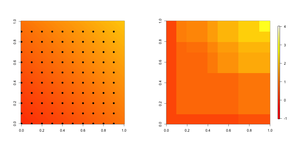
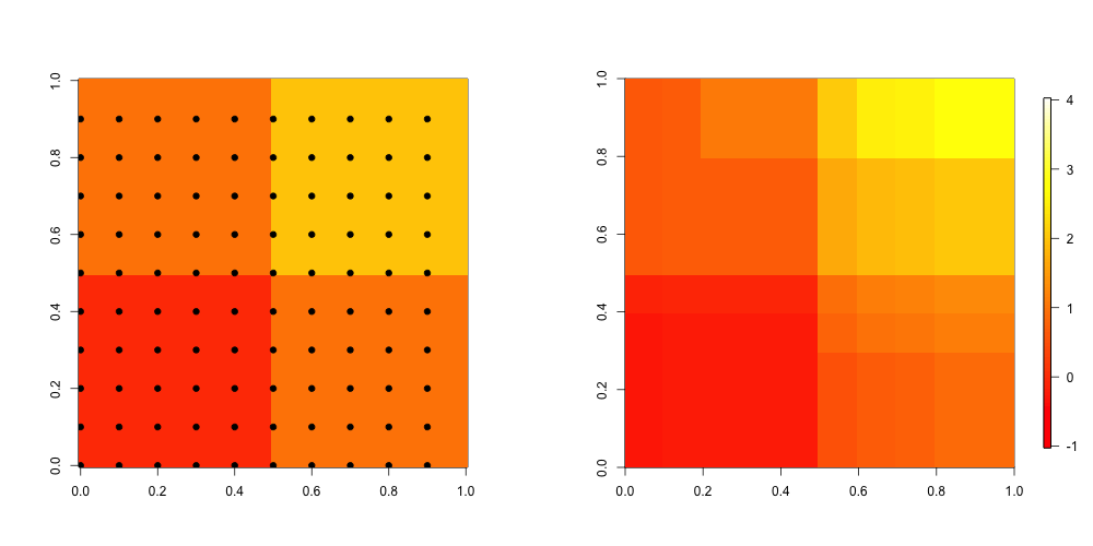
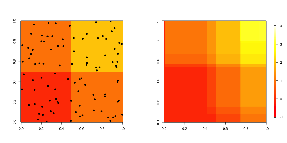
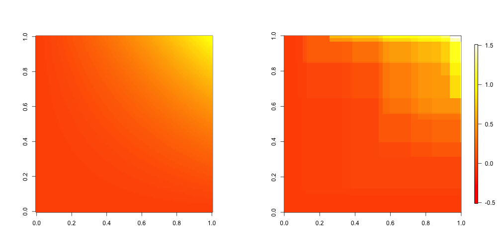
We start by visual illustrations of our estimators for specific values of $f^{*}$. In Figure 1 we depict an example of $\widehat{f}_{\textup{EM}}$ when fit on a $10\times 10$ grid of observations (i.e., $n_{1}=n_{2}=10$ and $n=100$) from an EM function $f^{*}$. In Figure 2, we consider a different example where $f^{*}$ has $k(f^{*})=4$ and depict the estimate $\widehat{f}_{\textup{EM}}$ computed on a $10\times 10$ grid of observations.

Figure 1: The function $f^{*}(x_{1},x_{2})=x_{1}+x_{2}$ (left), and the estimate $\widehat{f}_{\textup{EM}}$ (right) performed on observations from $f^{*}$ on the grid design ($n_{1}=n_{2}=10$) with standard Gaussian noise ($\sigma^{2}=1$).

Figure 2: The function $f^{*}(x_{1},x_{2})=\mathbb{I}\{x_{1}\geq 0.5\}+\mathbb{I}\{x_{2}\geq 0.5\}$ (left), and the estimate $\widehat{f}_{\textup{EM}}$ (right) performed on observations from $f^{*}$ with the grid design ($n_{1}=n_{2}=10$) and standard Gaussian noise ($\sigma^{2}=1$).

In Figure 3 we consider a function $f^{*}\in\mathfrak{R}^{d}_{1}(1/4)$ (see equations (71) and (72)) and depict our estimate $\widehat{f}_{\textup{HK}\boldsymbol{\mathbf{0}},V}$ computed from a $10\times 10$ grid of observations for various values of the tuning parameter $V$.

Figure 3: The function $f^{*}(x_{1},x_{2})=-\mathbb{I}\{x_{1}\geq 0.5,x_{2}\geq 0.5\}$ (upper left), and the estimate $\widehat{f}_{\textup{HK}\boldsymbol{\mathbf{0}},V}$ for $V=V^{*},2V^{*},3V^{*}$, performed on observations from $f^{*}$ on the grid design ($n_{1}=n_{2}=10$) with standard Gaussian noise ($\sigma^{2}=1$).

Figure 4: The function $f^{*}(x_{1},x_{2})=x_{1}+x_{2}$ (upper left), and the estimate $\widehat{f}_{\textup{HK}\boldsymbol{\mathbf{0}},V}$ for $V=V^{*},2V^{*},3V^{*}$, performed on observations from $f^{*}$ on the grid design ($n_{1}=n_{2}=10$) with standard Gaussian noise ($\sigma^{2}=1$).

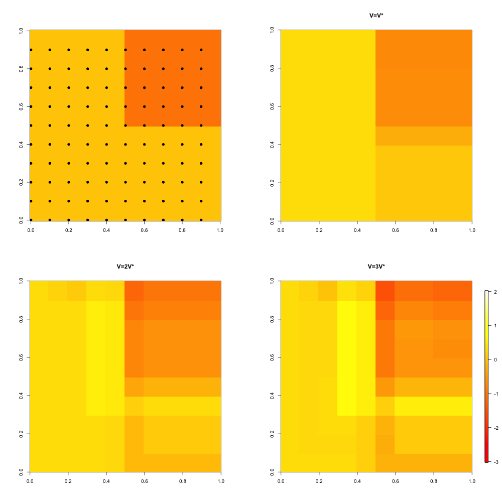
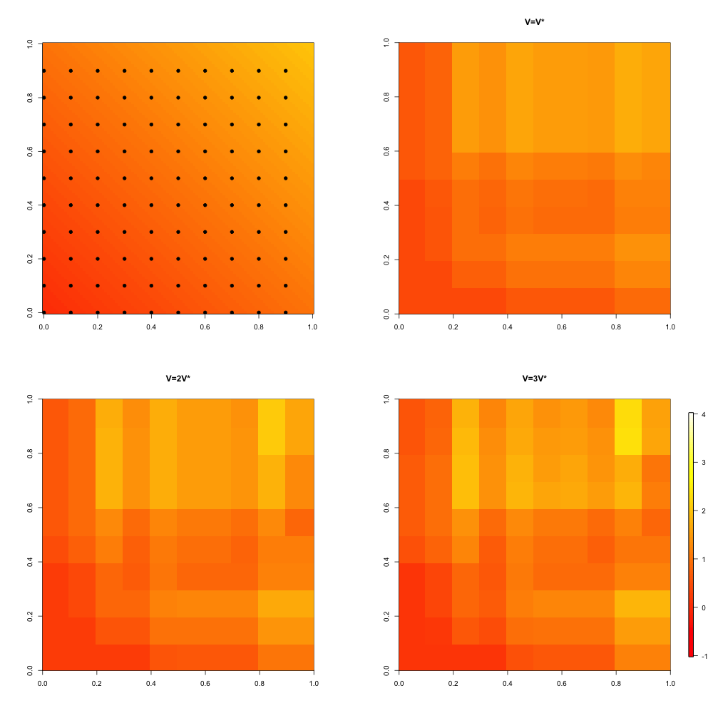
We remark that in these examples, we have chosen the estimator to be rectangular piecewise constant, with values obtained by solving the finite-dimensional NNLS or LASSO problem as discussed in Section 3. Additionally, one can observe in Figures 4 and 3 that the performance of $\widehat{f}_{\textup{HK}\boldsymbol{\mathbf{0}},V}$ improves as $V$ approaches the optimal $V^{*}$. Note also that in Figures 2 and 3 (in the case $V=V^{*}$) where $f^{*}$ is rectangular piecewise constant, the estimate is also rectangular piecewise constant with relatively few “jumps.”

Although our theorems in Section 4.1 and Section 4.2 only apply in case of lattice design, we can still compute the estimator for arbitrary design. In Figure 5, we used the “naïve gridding” approach described in Section 3 to compute the design matrix for the NNLS optimization problem. Note that the “jumps” in our estimate are located at design points.

Figure 5: The function $f^{*}(x_{1},x_{2})=\mathbb{I}\{x_{1}\geq 0.5\}+\mathbb{I}\{x_{2}\geq 0.5\}$ (left), and the estimate $\widehat{f}_{\textup{EM}}$ (right) performed on observations from $f^{*}$ on a uniformly drawn random design ($n=100$) and standard Gaussian noise ($\sigma^{2}=1$).

7.2 Bivariate current status model

One practical setting where our estimator may be useful is in the bivariate current status model, which is a particular variant of the interval censoring problem [33, 35, 48]. In this setting we observe $(\boldsymbol{\mathbf{x}}_{i},y_{i})$ where the $y_{i}$ are independent Bernoulli random variables $y_{i}$ with success parameter $F_{0}(\boldsymbol{\mathbf{x}}_{i})$, for some bivariate CDF $F_{0}$. Since $F_{0}$ is an entirely monotone function of $\boldsymbol{\mathbf{x}}$, it is plausible to use our EM estimator (2) on these observations to estimate $F_{0}$. In Figure 6, we simulated $n=500$ observations in the case where $F_{0}(\boldsymbol{\mathbf{x}})=\frac{1}{2}(x_{1}^{2}x_{2}+x_{1}x_{2}^{2})$ on $[0,1]^{2}$ (the CDF of the density $f_{0}(\boldsymbol{\mathbf{x}})=x_{1}+x_{2}$), and where $\boldsymbol{\mathbf{x}}_{i}$ are drawn uniformly from $[0,1]^{2}$, and where $y_{i}\mid\boldsymbol{\mathbf{x}}_{i}\sim\operatorname{Bern}(F_{0}(\boldsymbol{\mathbf{x}}_{i}))$. We get a fairly reasonable estimate of the original CDF on the interior of the square $[0,1]^{2}$. The estimated function is not a proper CDF, as it can take values outside of $[0,1]$, which happens often along the boundaries of the square $[0,1]^{2}$. One could avoid this by modifying the estimator $\widehat{f}_{\textup{EM}}$ by restricting the least squares optimization to functions in $\widehat{f}_{\textup{EM}}$ that take values in $[0,1]$, which would amount to adding two more linear constraints on the corresponding NNLS problem (37). This issue of obtaining an estimate that is not a proper CDF also occurs with a plug-in estimator studied by Groeneboom [33], which they address by proposing a truncation procedure on the boundaries of the square.

Figure 6: The CDF $F_{0}(x_{1},x_{2})=\frac{1}{2}(x_{1}x_{2}^{2}+x_{1}^{2}x_{2})$ (left), and the estimate $\widehat{f}_{\textup{EM}}$ (right) applied on $n=500$ observations of the form $(\boldsymbol{\mathbf{x}}_{i},y_{i})$ where $y_{i}\sim\operatorname{Bern}(F_{0}(\boldsymbol{\mathbf{x}}_{i}))$.

7.3 Adaptation to more general rectangular piecewise constant functions

One severe limitation of Theorems 4.7 and 6.1 is that they only consider functions of the form (71), which only has one “jump” and two continguous constant pieces.

The following simulation study suggests that the upper bound of $n^{-1}(\log n)^{\gamma}$ that we proved in Theorems 4.7 and 6.1 may also hold for a larger subclass of rectangular piecewise constant functions $\mathfrak{R}^{d}$.

The function $f^{*}:[0,1]^{2}\mapsto\mathbb{R}$ we consider is

$$f^{*}(\boldsymbol{\mathbf{x}})=\begin{cases}1&\boldsymbol{\mathbf{x}}\in\left([\frac{1}{3},\frac{2}{3})\times([0,\frac{1}{3})\cup[\frac{2}{3},1)\right)\cup\left(([0,\frac{1}{3})\cup[\frac{1}{3},1])\times[\frac{1}{3},\frac{2}{3})\right)\\ 0&\text{otherwise}.\end{cases}$$ (81)

One can check that $V^{*}=12$. Visually, it has a checkered pattern (see Figure 7).

Figure 7: Depiction of $f^{*}$ (left), and an example of $\widehat{f}_{\textup{HK}\boldsymbol{\mathbf{0}},V}$ (right) when given noisy measurements ($\sigma=0.5$) from $f^{*}$ on the grid design ($n_{1}=n_{2}=50$).

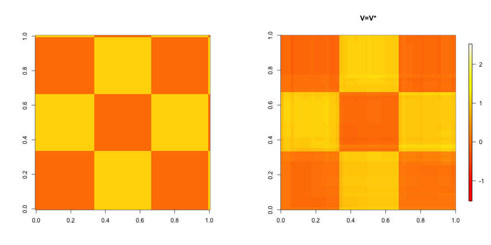
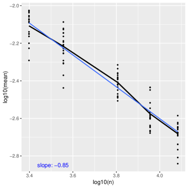
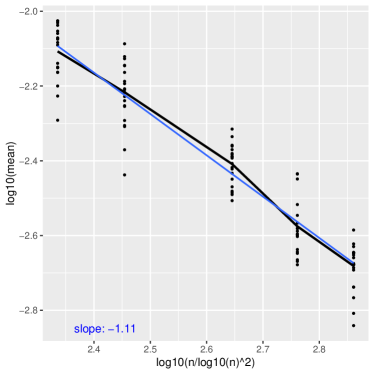
We considered the lattice design $\mathbb{L}_{n_{1},\ldots,n_{d}}$ with $n_{1}=n_{2}\in\{50,60,80,95,110\}$ (note that consequently $n=n_{1}n_{2}$ ranges between $2500$ and $12100$). For each value of $n$, we performed $20$ trials of generating observations $y_{1},\ldots,y_{n}$ with noise $\sigma=0.5$, computed $\widehat{f}_{\textup{HK}\boldsymbol{\mathbf{0}},V}$ with $V=V^{*}$, and computed the error $\frac{1}{n}\sum_{i=1}^{n}(\widehat{f}_{\textup{HK}\boldsymbol{\mathbf{0}},V}(\boldsymbol{\mathbf{x}}_{i})-f^{*}(\boldsymbol{\mathbf{x}}_{i}))^{2}$. Averaging over the $20$ trials gives us an estimate $r_{n}$ of $\mathcal{R}(\widehat{f}_{\textup{HK}\boldsymbol{\mathbf{0}},V},f^{*})$ for that value of $n$.

As shown in Figure 8 A linear regression of $\log r_{n}$ over $\log n$ yielded a slope of $-0.85$ which indicates that the estimator is performing better than the worst-case rate of $n^{-2/3}$ given in Theorem 4.5. A linear regression of $\log r_{n}$ over $\log\frac{n}{\log n}$ yielded a slope of $-0.96$, while a regression of $\log r_{n}$ over $\log\frac{n}{(\log n)^{2}}$ yielded a slope of $-1.11$. Thus these simulations suggest that the estimator $\widehat{f}_{\textup{HK}\boldsymbol{\mathbf{0}},V}$ has risk on the order of $n^{-1}(\log n)^{\gamma}$ (possibly for $\gamma\leq 2$) for rectangular piecewise constant functions beyond the ones considered in Theorems 4.7 and 6.1.

Figure 8: Plot of estimate of $\log\mathcal{R}(\widehat{f}_{\textup{HK}\boldsymbol{\mathbf{0}},V},f^{*})$ vs. $\log n$ (left) and vs. $\log\frac{n}{(\log n)^{2}}$ (right).

8 Proofs of Risk Results

8.1 Preliminaries

Note that the risks $\mathcal{R}(\widehat{f}_{\textup{EM}},f^{*})$ and $\mathcal{R}(\widehat{f}_{\textup{HK}\boldsymbol{\mathbf{0}},V},f^{*})$ both only depend on the values of the estimators $\widehat{f}_{\textup{EM}}$ and $\widehat{f}_{\textup{HK}\boldsymbol{\mathbf{0}},V}$ at the design points $\boldsymbol{\mathbf{x}}_{1},\dots,\boldsymbol{\mathbf{x}}_{n}$. Also by the results from Section 3, it is clear that the vectors $(\widehat{f}_{\textup{EM}}(\boldsymbol{\mathbf{x}}_{1}),\dots,\widehat{f}_{\textup{EM}}(\boldsymbol{\mathbf{x}}_{n}))$ and $(\widehat{f}_{\textup{HK}\boldsymbol{\mathbf{0}},V}(\boldsymbol{\mathbf{x}}_{1}),\dots,\widehat{f}_{\textup{HK}\boldsymbol{\mathbf{0}},V}(\boldsymbol{\mathbf{x}}_{n}))$ are Euclidean projections of the data vector $\boldsymbol{\mathbf{y}}=(y_{1},\dots,y_{n})$ on the closed convex sets

$$\left\{\boldsymbol{\mathbf{A}}\boldsymbol{\mathbf{\beta}}:\min_{j\geq 2}\beta_{j}\geq 0\right\}~{}~{}\text{ and }~{}~{}\left\{\boldsymbol{\mathbf{A}}\boldsymbol{\mathbf{\beta}}:\sum_{j\geq 2}|\beta_{j}|\leq V\right\}$$

respectively. Consequently, we can apply general results from the theory of convex-constrained LSEs to prove the risk results for $\widehat{f}_{\textup{EM}}$ and $\widehat{f}_{\textup{HK}\boldsymbol{\mathbf{0}},V}$. This theory is, by now, well established (see e.g., van de Geer [67], van der Vaart and Wellner [72], Hjort and Pollard [41], Chatterjee [14]). The following result from Chatterjee [14] provides upper bounds for the risk of general convex-constrained LSEs. This result will be used in the proofs of Theorem 4.1 and Theorem 4.5.

Theorem 8.1 (Chatterjee [14]).

Let $\mathcal{K}$ be a closed convex set in $\mathbb{R}^{n}$ and let

$$\boldsymbol{\mathbf{\widehat{\boldsymbol{\mathbf{\theta}}}}}\coloneqq\operatorname*{\arg\!\min}_{\boldsymbol{\mathbf{\theta}}\in\mathcal{K}}\|\boldsymbol{\mathbf{y}}-\boldsymbol{\mathbf{\theta}}\|^{2},$$ (82)

where $\boldsymbol{\mathbf{y}}\sim\mathcal{N}_{n}(\boldsymbol{\mathbf{\boldsymbol{\mathbf{\theta}}}}^{*},\boldsymbol{\mathbf{I}}_{n})$ for some $\boldsymbol{\mathbf{\boldsymbol{\mathbf{\theta}}}}^{*}\in\mathbb{R}^{n}$ (not necessarily in $\mathcal{K}$). Then there exists a universal positive constant $C$ such that

$$\mathbb{E}\|\boldsymbol{\mathbf{\widehat{\boldsymbol{\mathbf{\theta}}}}}-\boldsymbol{\mathbf{\boldsymbol{\mathbf{\theta}}}}^{*}\|^{2}\leq C\max(t_{*}^{2},1)$$ (83)

for every $t_{*}>0$ which satisfies

$$\mathbb{E}\left[\sup_{\boldsymbol{\mathbf{\theta}}\in\mathcal{K}:\|\boldsymbol{\mathbf{\theta}}-\boldsymbol{\mathbf{\boldsymbol{\mathbf{\theta}}}}^{*}\|\leq t_{*}}\langle\boldsymbol{\mathbf{\xi}},\boldsymbol{\mathbf{\theta}}-\boldsymbol{\mathbf{\boldsymbol{\mathbf{\theta}}}}^{*}\rangle\right]\leq\frac{t_{*}^{2}}{2}\qquad\text{where $\boldsymbol{\mathbf{\xi}}\sim\mathcal{N}_{n}(\boldsymbol{\mathbf{0}},\boldsymbol{\mathbf{I}}_{n})$}.$$ (84)

Theorem 8.1 is sufficient to prove Theorem 4.1 and Theorem 4.5. However, in order to handle the misspecified setting discussed in 4.1 and 4.3, one needs the following generalization of Theorem 8.1. Below,

$$\Pi_{\mathcal{K}}(\boldsymbol{\mathbf{v}})\coloneqq\operatorname*{\arg\!\min}_{\boldsymbol{\mathbf{\theta}}\in\mathcal{K}}\|\boldsymbol{\mathbf{v}}-\boldsymbol{\mathbf{\theta}}\|^{2}$$ (85)

denotes the projection of $\boldsymbol{\mathbf{v}}$ onto the closed convex set $\mathcal{K}$. The following result generalizes Theorem 8.1 to the case of model misspecification. It is similar to related generalizations of Theorem 8.1 from Chen et al. [18] and Bellec [7]. We omit the proof of this result as it can be proved by a straightforward generalization of the proof of the original result, Theorem 8.1, from Chatterjee [14].

Theorem 8.2.

Let $\mathcal{K}$ be a closed convex set in $\mathbb{R}^{n}$, and let $\boldsymbol{\mathbf{\widehat{\boldsymbol{\mathbf{\theta}}}}}\coloneqq\Pi_{\mathcal{K}}(\boldsymbol{\mathbf{y}})$ be as defined above (82), with $\boldsymbol{\mathbf{y}}\sim\mathcal{N}_{n}(\boldsymbol{\mathbf{\boldsymbol{\mathbf{\theta}}}}^{*},\boldsymbol{\mathbf{I}}_{n})$ and $\boldsymbol{\mathbf{\boldsymbol{\mathbf{\theta}}}}^{*}\in\mathbb{R}^{n}$. Then there exists a universal positive constant $C$ such that

$$\mathbb{E}\|\boldsymbol{\mathbf{\widehat{\boldsymbol{\mathbf{\theta}}}}}-\Pi_{\mathcal{K}}(\boldsymbol{\mathbf{\boldsymbol{\mathbf{\theta}}}}^{*})\|^{2}\leq C\max(t_{*}^{2},1),$$ (86)

for every $t_{*}>0$ which satisfies

$$\mathbb{E}\left[\sup_{\boldsymbol{\mathbf{\theta}}\in\mathcal{K}:\|\boldsymbol{\mathbf{\theta}}-\Pi_{\mathcal{K}}(\boldsymbol{\mathbf{\boldsymbol{\mathbf{\theta}}}}^{*})\|\leq t_{*}}\langle\boldsymbol{\mathbf{\xi}},\boldsymbol{\mathbf{\theta}}-\Pi_{\mathcal{K}}(\boldsymbol{\mathbf{\boldsymbol{\mathbf{\theta}}}}^{*})\rangle\right]\leq\frac{t_{*}^{2}}{2}\qquad\text{where $\boldsymbol{\mathbf{\xi}}\sim\mathcal{N}_{n}(0,\boldsymbol{\mathbf{I}}_{n})$}.$$ (87)

Note that in the well-specified setting $\boldsymbol{\mathbf{\boldsymbol{\mathbf{\theta}}}}^{*}\in\mathcal{K}$, we have $\Pi_{\mathcal{K}}(\boldsymbol{\mathbf{\boldsymbol{\mathbf{\theta}}}}^{*})=\boldsymbol{\mathbf{\boldsymbol{\mathbf{\theta}}}}^{*}$, and thus Theorem 8.1 and Theorem 8.2 are identical. On the other hand, in the misspecified setting $\boldsymbol{\mathbf{\boldsymbol{\mathbf{\theta}}}}^{*}\notin\mathcal{K}$, the two results differ in the risk quantity they control: $\mathbb{E}\|\boldsymbol{\mathbf{\widehat{\boldsymbol{\mathbf{\theta}}}}}-\boldsymbol{\mathbf{\boldsymbol{\mathbf{\theta}}}}^{*}\|^{2}$ and $\mathbb{E}\|\boldsymbol{\mathbf{\widehat{\boldsymbol{\mathbf{\theta}}}}}-\Pi_{\mathcal{K}}(\boldsymbol{\mathbf{\boldsymbol{\mathbf{\theta}}}}^{*})\|^{2}$ respectively and the fact that $\boldsymbol{\mathbf{\boldsymbol{\mathbf{\theta}}}}^{*}$ appearing in (84) is replaced by $\Pi_{\mathcal{K}}(\boldsymbol{\mathbf{\boldsymbol{\mathbf{\theta}}}}^{*})$ in (87).

Remark 8.1 (Risk bounds under misspecification).

Theorem 4.1 and Theorem 4.5 are proved via Theorem 8.1 by establishing (84) for an appropriate $t_{*}$. If we replace $\boldsymbol{\mathbf{\boldsymbol{\mathbf{\theta}}}}^{*}$ in these proofs by $\Pi_{\mathcal{K}}(\boldsymbol{\mathbf{\boldsymbol{\mathbf{\theta}}}}^{*})$ and replace the use of Theorem 8.1 with that of Theorem 8.2, we obtain the risk bounds under misspecification described in 4.1 and 4.3.

The risk of the estimator $\boldsymbol{\mathbf{\widehat{\boldsymbol{\mathbf{\theta}}}}}$ in (82) can also be related to the tangent cones of the closed convex set $K$ at $\boldsymbol{\mathbf{\boldsymbol{\mathbf{\theta}}}}^{*}$. To describe these results, we need some notation and terminology. The tangent cone of $\mathcal{K}$ at $\boldsymbol{\mathbf{\theta}}\in\mathcal{K}$ is defined as

$$\mathcal{T}_{\mathcal{K}}(\boldsymbol{\mathbf{\theta}})\{t(\boldsymbol{\mathbf{\eta}}-\boldsymbol{\mathbf{\theta}}):t\geq 0,\boldsymbol{\mathbf{\eta}}\in\mathcal{K}\}.$$ (88)

Informally, $\mathcal{T}_{\mathcal{K}}(\boldsymbol{\mathbf{\theta}})$ represents all directions in which one can move from $\boldsymbol{\mathbf{\theta}}$ and still remain in $K$. Note that $\mathcal{T}_{\mathcal{K}}(\boldsymbol{\mathbf{\theta}})$ is a cone which means that $a\boldsymbol{\mathbf{\alpha}}\in\mathcal{T}_{\mathcal{K}}(\boldsymbol{\mathbf{\theta}})$ for every $\boldsymbol{\mathbf{\alpha}}\in\mathcal{T}_{\mathcal{K}}(\boldsymbol{\mathbf{\theta}})$ and $a\geq 0$. It is also easy to see that $\mathcal{T}_{\mathcal{K}}(\boldsymbol{\mathbf{\theta}})$ closed and convex.

The statistical dimension of a closed convex cone $\mathcal{T}\subseteq\mathbb{R}^{n}$ is defined as

$$\delta(\mathcal{T})\coloneqq\mathbb{E}\|\Pi_{\mathcal{T}}(Z)\|^{2},\qquad\text{where $Z\sim\mathcal{N}_{n}(0,\boldsymbol{\mathbf{I}}_{n})$}$$ (89)

and $\Pi_{\mathcal{T}}(Z)\coloneqq\operatorname*{\arg\!\min}_{\boldsymbol{\mathbf{u}}\in\mathcal{T}}\|Z-\boldsymbol{\mathbf{u}}\|^{2}$ is the projection of $Z$ onto $T$. The terminology of statistical dimension is due to Amelunxen et al. [2] and we refer the reader to this paper for many properties of the statistical dimension.

The relevance of these notions to the estimator $\boldsymbol{\mathbf{\widehat{\boldsymbol{\mathbf{\theta}}}}}$ (defined in (82)) is that the risk of $\boldsymbol{\mathbf{\widehat{\boldsymbol{\mathbf{\theta}}}}}$ can be related to the statistical dimension of tangent cones of $K$. This is the content of the following result due to Bellec [8, Corollary 2.2].

Theorem 8.3.

Suppose $Y\sim\mathcal{N}_{n}(\boldsymbol{\mathbf{\boldsymbol{\mathbf{\theta}}}}^{*},\sigma^{2}\boldsymbol{\mathbf{I}}_{n})$ for some $\boldsymbol{\mathbf{\boldsymbol{\mathbf{\theta}}}}^{*}\in\mathbb{R}^{n}$ and $\sigma^{2}>0$ and consider the estimator $\boldsymbol{\mathbf{\widehat{\boldsymbol{\mathbf{\theta}}}}}$ defined in (82) for a closed convex set $K$. Then

$$\mathbb{E}\|\boldsymbol{\mathbf{\widehat{\boldsymbol{\mathbf{\theta}}}}}-\boldsymbol{\mathbf{\boldsymbol{\mathbf{\theta}}}}^{*}\|^{2}\leq\inf_{\boldsymbol{\mathbf{\theta}}\in\mathcal{K}}\left[\|\boldsymbol{\mathbf{\theta}}-\boldsymbol{\mathbf{\boldsymbol{\mathbf{\theta}}}}^{*}\|^{2}+\sigma^{2}\delta(\mathcal{T}_{\mathcal{K}}(\boldsymbol{\mathbf{\theta}}))\right].$$ (90)

The statistical dimension $\delta(\mathcal{T})$ of a closed convex cone $\mathcal{T}$ is closely related to the Gaussian width of $\mathcal{T}$ which is defined as

$$w(\mathcal{T})\coloneqq\mathbb{E}\left[\sup_{\boldsymbol{\mathbf{\theta}}\in\mathcal{T}:\|\boldsymbol{\mathbf{\theta}}\|\leq 1}\langle Z,\boldsymbol{\mathbf{\theta}}\rangle\right]\qquad\text{where $Z\sim\mathcal{N}_{n}(0,\boldsymbol{\mathbf{I}}_{n})$}.$$ (91)

Indeed, it has been shown in Amelunxen et al. [2, Proposition 10.2] that

$$w^{2}(\mathcal{T})\leq\delta(\mathcal{T})\leq w^{2}(\mathcal{T})+1$$ (92)

for every closed convex cone $T$. Using this relation in conjunction with (90), we obtain the following bound on the risk of the estimator $\boldsymbol{\mathbf{\widehat{\boldsymbol{\mathbf{\theta}}}}}$ defined in (82) when $Y\sim\mathcal{N}_{n}(\boldsymbol{\mathbf{\boldsymbol{\mathbf{\theta}}}}^{*},\sigma^{2}\boldsymbol{\mathbf{I}}_{n})$:

$$\mathbb{E}\|\boldsymbol{\mathbf{\widehat{\boldsymbol{\mathbf{\theta}}}}}-\boldsymbol{\mathbf{\boldsymbol{\mathbf{\theta}}}}^{*}\|^{2}\leq\inf_{\boldsymbol{\mathbf{\theta}}\in K}\left[\|\boldsymbol{\mathbf{\theta}}-\boldsymbol{\mathbf{\boldsymbol{\mathbf{\theta}}}}^{*}\|^{2}+\sigma^{2}+\sigma^{2}w^{2}(T_{K}(\boldsymbol{\mathbf{\theta}}))\right].$$ (93)

8.2 Proof of Theorem 4.1

Let

$$\boldsymbol{\mathbf{\widehat{\boldsymbol{\mathbf{\theta}}}}}\coloneqq(\widehat{f}_{\textup{EM}}(\boldsymbol{\mathbf{x}}_{1}),\ldots,\widehat{f}_{\textup{EM}}(\boldsymbol{\mathbf{x}}_{n}))~{}~{}\text{ and }~{}~{}\boldsymbol{\mathbf{\boldsymbol{\mathbf{\theta}}}}^{*}\coloneqq(f^{*}(\boldsymbol{\mathbf{x}}_{1}),\ldots,f^{*}(\boldsymbol{\mathbf{x}}_{n}))$$ (94)

and note that

$$\mathcal{R}(\widehat{f}_{\textup{EM}},f^{*})=\mathbb{E}\frac{1}{n}\|\boldsymbol{\mathbf{\widehat{\boldsymbol{\mathbf{\theta}}}}}-\boldsymbol{\mathbf{\boldsymbol{\mathbf{\theta}}}}^{*}\|^{2}$$

where $\|\cdot\|$ denotes the usual Euclidean norm in $\mathbb{R}^{n}$.

Observe that by 3.1, it follows that $\boldsymbol{\mathbf{\widehat{\boldsymbol{\mathbf{\theta}}}}}=\boldsymbol{\mathbf{A}}\boldsymbol{\mathbf{\widehat{\beta}}}_{\textup{EM}}$ is the projection of the data vector $\boldsymbol{\mathbf{y}}$ on the closed convex cone

$$\mathcal{D}_{n_{1},\ldots,n_{d}}\coloneqq\{\boldsymbol{\mathbf{A}}\boldsymbol{\mathbf{\beta}}:\beta_{j}\geq 0,\forall j\geq 2\}=\{(f(\boldsymbol{\mathbf{x}}_{1}),\dots,f(\boldsymbol{\mathbf{x}}_{n})):f\in\mathcal{F}_{\textup{EM}}^{d}\}.$$ (95)

where $\boldsymbol{\mathbf{A}}$ is the design matrix introduced in Section 3. Note that, under the lattice design (46), the set $\mathcal{D}_{n_{1},\ldots,n_{d}}$ is completely determined by the values of $n_{1},\ldots,n_{d}$. We can therefore employ Theorem 8.1 to bound the risk $\mathbb{E}\|\boldsymbol{\mathbf{\widehat{\boldsymbol{\mathbf{\theta}}}}}-\boldsymbol{\mathbf{\boldsymbol{\mathbf{\theta}}}}^{*}\|^{2}/n$.

First, we claim that it suffices to prove the theorem under the assumption $n_{j}\geq 2$ for all $j=1,\ldots,d$. To see this, note first that when $n=n_{1}\cdots n_{d}=1$, we have $\boldsymbol{\mathbf{\widehat{\boldsymbol{\mathbf{\theta}}}}}=\boldsymbol{\mathbf{y}}$ so that $\mathcal{R}(\boldsymbol{\mathbf{\widehat{\boldsymbol{\mathbf{\theta}}}}},\boldsymbol{\mathbf{\boldsymbol{\mathbf{\theta}}}}^{*})=\sigma^{2}/n$ and the result holds which means that we can assume that $\max_{j}n_{j}\geq 2$ for some $j$. Now if $n_{j}=1$ for some values of $j$, we can simply ignore these components and focus on the equivalent problem with a lattice design (46) in a lower-dimensional space that has at least two grid points in each component. We can apply the bound (59) to this lower-dimensional problem (for instance, the dimension would be $d^{\prime}=\#\{j:n_{j}\geq 2\}$ instead of $d$) and then remark that the bound (59) for the original problem is even larger.

Next, we claim that it suffices to prove the theorem under the assumption $\sigma^{2}=1$. Indeed in general we may consider the rescaled problem with $\widetilde{f}\coloneqq f^{*}/\sigma$, $\widetilde{V}^{*}\coloneqq V^{*}/\sigma$, and $\widetilde{y}_{i}\sim\mathcal{N}(\widetilde{f}(\boldsymbol{\mathbf{x}}_{i}),1)$, apply the bound (59), and then multiply the risk bound by $\sigma^{2}$ to account for rescaling the fitted function by $\sigma$. This is possible because $\mathcal{F}_{\textup{EM}}^{d}$ is a cone.

So, we assume $n_{j}\geq 2$ for all $j=1,\ldots,d$ and $\sigma^{2}=1$. As mentioned above, we want to bound $\mathbb{E}\|\boldsymbol{\mathbf{\widehat{\boldsymbol{\mathbf{\theta}}}}}-\boldsymbol{\mathbf{\boldsymbol{\mathbf{\theta}}}}^{*}\|^{2}/n$ using Theorem 8.1. For this, we need to obtain upper bounds for

$$G(t)\coloneqq\mathbb{E}\sup_{\boldsymbol{\mathbf{\theta}}\in\mathcal{D}_{n_{1},\ldots,n_{d}}\cap\mathcal{B}_{2}(\boldsymbol{\mathbf{\boldsymbol{\mathbf{\theta}}}}^{*},t)}\langle\boldsymbol{\mathbf{\xi}},\boldsymbol{\mathbf{\theta}}-\boldsymbol{\mathbf{\boldsymbol{\mathbf{\theta}}}}^{*}\rangle$$ (96)

where $\boldsymbol{\mathbf{\xi}}\sim\mathcal{N}_{n}(0,\boldsymbol{\mathbf{I}}_{n})$ and $\mathcal{B}_{2}(\boldsymbol{\mathbf{\boldsymbol{\mathbf{\theta}}}}^{*},t)\coloneqq\{\boldsymbol{\mathbf{\theta}}:\|\boldsymbol{\mathbf{\theta}}-\boldsymbol{\mathbf{\boldsymbol{\mathbf{\theta}}}}^{*}\|<t\}$ denotes the ball of radius $t$ centered at $\boldsymbol{\mathbf{\boldsymbol{\mathbf{\theta}}}}^{*}$.

In what follows, we sometimes treat vectors in $\mathbb{R}^{n}$ as arrays in $\mathbb{R}^{n_{1}\times\cdots\times n_{d}}$ indexed by $\boldsymbol{\mathbf{i}}=(i_{1},\ldots,i_{d})$ for $0\leq i_{j}\leq n_{j}-1$ and $j=1,\ldots,d$.

For each $j\in 1,\ldots,d$, let

$$S^{(0)}_{j}\coloneqq\{i_{j}:0\leq i_{j}\leq\frac{n_{j}}{2}-1\},\qquad S^{(1)}_{j}\coloneqq\{i_{j}:\frac{n_{j}}{2}-1<i_{j}\leq n_{j}-1\},$$ (97)

so that

$$\langle\boldsymbol{\mathbf{\xi}},\boldsymbol{\mathbf{\theta}}-\boldsymbol{\mathbf{\boldsymbol{\mathbf{\theta}}}}^{*}\rangle =\sum_{i_{1}=0}^{n_{1}-1}\cdots\sum_{i_{d}=0}^{n_{d}-1}\xi_{\boldsymbol{\mathbf{i}}}(\theta_{\boldsymbol{\mathbf{i}}}-\theta^{*}_{\boldsymbol{\mathbf{i}}})=\sum_{\boldsymbol{\mathbf{z}}\in\{0,1\}^{d}}\sum_{\boldsymbol{\mathbf{i}}\in S_{1}^{(z_{1})}\times\cdots\times S_{d}^{(z_{d})}}\xi_{\boldsymbol{\mathbf{i}}}(\theta_{\boldsymbol{\mathbf{i}}}-\theta^{*}_{\boldsymbol{\mathbf{i}}}).$$ (98)

We then obtain the bound

$$G(t)\leq\sum_{\boldsymbol{\mathbf{z}}\in\{0,1\}^{d}}\underbrace{\mathbb{E}\sup_{\boldsymbol{\mathbf{\theta}}\in\mathcal{D}_{n_{1},\ldots,n_{d}}\cap\mathcal{B}_{2}(\boldsymbol{\mathbf{\boldsymbol{\mathbf{\theta}}}}^{*},t)}\sum_{\boldsymbol{\mathbf{i}}\in S_{1}^{(z_{1})}\times\cdots\times S_{d}^{(z_{d})}}\xi_{\boldsymbol{\mathbf{i}}}(\theta_{\boldsymbol{\mathbf{i}}}-\theta^{*}_{\boldsymbol{\mathbf{i}}})}_{\eqqcolon H_{\boldsymbol{\mathbf{z}}}(t)}.$$ (99)

We now bound $H_{\boldsymbol{\mathbf{z}}}(t)$ for fixed $\boldsymbol{\mathbf{z}}\in\{0,1\}^{d}$. For each $j=1,\ldots,d$ let $K_{j}$ denote the largest positive integer $k_{j}$ for which

$$\left\{i_{j}\in S^{(z_{j})}_{j}n_{j}2^{-(k_{j}+1)}-1+z_{j}n_{j}/2<i_{j}\leq n_{j}2^{-k_{j}}-1+z_{j}n_{j}/2\right\}$$ (100)

is nonempty. Let $\mathcal{K}\coloneqq\bigtimes_{j=1}^{d}\{1,\ldots,K_{j}\}$ and note that $|\mathcal{K}|=K_{1}K_{2}\cdots K_{d}$. For $\boldsymbol{\mathbf{k}}\coloneqq(k_{1},\ldots,k_{d})\in\mathcal{K}$ and $\boldsymbol{\mathbf{\theta}}\in\mathbb{R}^{n_{1}\times\cdots\times n_{d}}$, let

$$\boldsymbol{\mathbf{\theta}}^{(\boldsymbol{\mathbf{k}})} \coloneqq\Big{\{}\boldsymbol{\mathbf{\theta}}_{\boldsymbol{\mathbf{i}}}:n_{j}2^{-(k_{j}+1)}-1+z_{j}n_{j}/2<i_{j}\leq n_{j}2^{-k_{j}}-1+z_{j}n_{j}/2,\,$$ (101)

$$\qquad\qquad\qquad i_{j}=0,\ldots,n_{j}-1,\,j=1,\ldots,d\Big{\}}.$$ (102)

Let $\mathcal{M}\coloneqq\{(m_{\boldsymbol{\mathbf{k}}})_{\boldsymbol{\mathbf{k}}\in\mathcal{K}}:1\leq m_{\boldsymbol{\mathbf{k}}}\leq|\mathcal{K}|,\sum_{\boldsymbol{\mathbf{k}}\in\mathcal{K}}m_{\boldsymbol{\mathbf{k}}}\leq 2|\mathcal{K}|\}$. For $\boldsymbol{\mathbf{m}}\in\mathcal{M}$, we define

$$T_{\boldsymbol{\mathbf{m}}}(t)\coloneqq\left\{\boldsymbol{\mathbf{\theta}}\in\mathcal{D}_{n_{1},\ldots,n_{d}}\cap\mathcal{B}_{2}(\boldsymbol{\mathbf{\boldsymbol{\mathbf{\theta}}}}^{*},t):\|\boldsymbol{\mathbf{\theta}}-\boldsymbol{\mathbf{\boldsymbol{\mathbf{\theta}}}}^{*}\|\leq t,\|\boldsymbol{\mathbf{\theta}}^{(\boldsymbol{\mathbf{k}})}-(\boldsymbol{\mathbf{\boldsymbol{\mathbf{\theta}}}}^{*})^{(\boldsymbol{\mathbf{k}})}\|^{2}\leq\frac{m_{\boldsymbol{\mathbf{k}}}t^{2}}{|\mathcal{K}|},\forall\boldsymbol{\mathbf{k}}\in\mathcal{K}\right\}.$$ (103)

We claim

$$\mathcal{D}_{n_{1},\ldots,n_{d}}\cap\mathcal{B}_{2}(\boldsymbol{\mathbf{\boldsymbol{\mathbf{\theta}}}}^{*},t)\subseteq\bigcup_{\boldsymbol{\mathbf{m}}\in\mathcal{M}}T_{\boldsymbol{\mathbf{m}}}(t).$$ (104)

Indeed suppose $\boldsymbol{\mathbf{\theta}}\in\mathcal{D}_{n_{1},\ldots,n_{d}}\cap\mathcal{B}_{2}(\boldsymbol{\mathbf{\boldsymbol{\mathbf{\theta}}}}^{*},t)$; then we have $t^{2}\geq\|\boldsymbol{\mathbf{\theta}}-\boldsymbol{\mathbf{\boldsymbol{\mathbf{\theta}}}}^{*}\|^{2}\geq\|\boldsymbol{\mathbf{\theta}}^{(\boldsymbol{\mathbf{k}})}-(\boldsymbol{\mathbf{\boldsymbol{\mathbf{\theta}}}}^{*})^{(\boldsymbol{\mathbf{k}})}\|^{2}$ for each $\boldsymbol{\mathbf{k}}$, and thus there exists $1\leq m_{\boldsymbol{\mathbf{k}}}\leq|\mathcal{K}|$ such that

$$m_{\boldsymbol{\mathbf{k}}}-1\leq|\mathcal{K}|\frac{\|\boldsymbol{\mathbf{\theta}}^{(\boldsymbol{\mathbf{k}})}-(\boldsymbol{\mathbf{\boldsymbol{\mathbf{\theta}}}}^{*})^{(\boldsymbol{\mathbf{k}})}\|^{2}}{t^{2}}\leq m_{\boldsymbol{\mathbf{k}}}.$$ (105)

This implies

$$1\geq t^{-2}\|\boldsymbol{\mathbf{\theta}}-\boldsymbol{\mathbf{\boldsymbol{\mathbf{\theta}}}}^{*}\|^{2}\geq t^{-2}\sum_{\boldsymbol{\mathbf{k}}\in\mathcal{K}}\|\boldsymbol{\mathbf{\theta}}^{(\boldsymbol{\mathbf{k}})}-(\boldsymbol{\mathbf{\boldsymbol{\mathbf{\theta}}}}^{*})^{(\boldsymbol{\mathbf{k}})}\|^{2}\geq|\mathcal{K}|^{-1}\sum_{\boldsymbol{\mathbf{k}}\in\mathcal{K}}(m_{\boldsymbol{\mathbf{k}}}-1)$$ (106)

and thus $\sum_{\boldsymbol{\mathbf{k}}\in\mathcal{K}}m_{\boldsymbol{\mathbf{k}}}\leq 2|\mathcal{K}|$, so $\boldsymbol{\mathbf{m}}\in\mathcal{M}$ and $\boldsymbol{\mathbf{\theta}}\in T_{\boldsymbol{\mathbf{m}}}(t)$, which verifies the claim (104).

Using this claim (104) we obtain

$$H_{\boldsymbol{\mathbf{z}}}(t)\leq\mathbb{E}\max_{\boldsymbol{\mathbf{m}}\in\mathcal{M}}\sup_{\boldsymbol{\mathbf{\theta}}\in T_{\boldsymbol{\mathbf{m}}}}\sum_{\boldsymbol{\mathbf{i}}\in S_{1}^{(z_{1})}\times\cdots\times S_{d}^{(z_{d})}}\xi_{\boldsymbol{\mathbf{i}}}(\theta_{\boldsymbol{\mathbf{i}}}-\theta^{*}_{\boldsymbol{\mathbf{i}}}).$$ (107)

Lemma D.1 from [37] then implies

$$H_{\boldsymbol{\mathbf{z}}}(t)\leq\max_{\boldsymbol{\mathbf{m}}\in\mathcal{M}}\mathbb{E}\sup_{\boldsymbol{\mathbf{\theta}}\in T_{\boldsymbol{\mathbf{m}}}(t)}\sum_{\boldsymbol{\mathbf{i}}\in S_{1}^{(z_{1})}\times\cdots\times S_{d}^{(z_{d})}}\xi_{\boldsymbol{\mathbf{i}}}(\theta_{\boldsymbol{\mathbf{i}}}-\theta^{*}_{\boldsymbol{\mathbf{i}}})+t\sqrt{2\log|\mathcal{M}|}+t\sqrt{\pi/2}.$$ (108)

Because the number of $|\mathcal{K}|$-tuples of positive integers summing to $p$ is $\binom{p-1}{|\mathcal{K}|-1}=\binom{p-1}{p-|\mathcal{K}|}$, we can bound the cardinality of $\mathcal{M}$ by

$$|\mathcal{M}|\leq\sum_{p=|\mathcal{K}|}^{2|\mathcal{K}|}\binom{p-1}{p-|\mathcal{K}|}\leq\sum_{p=|\mathcal{K}|}^{2|\mathcal{K}|}\binom{2|\mathcal{K}|-1}{p-|\mathcal{K}|}\leq 2^{2|\mathcal{K}|-1}.$$ (109)

Thus,

$$H_{\boldsymbol{\mathbf{z}}}(t)\leq\max_{\boldsymbol{\mathbf{m}}\in\mathcal{M}}\underbrace{\mathbb{E}\sup_{\boldsymbol{\mathbf{\theta}}\in T_{\boldsymbol{\mathbf{m}}}(t)}\sum_{\boldsymbol{\mathbf{i}}\in S_{1}^{(z_{1})}\times\cdots\times S_{d}^{(z_{d})}}\xi_{\boldsymbol{\mathbf{i}}}(\theta_{\boldsymbol{\mathbf{i}}}-\theta^{*}_{\boldsymbol{\mathbf{i}}})}_{\eqqcolon U_{\boldsymbol{\mathbf{z}},\boldsymbol{\mathbf{m}}}(t)}+2t\sqrt{|\mathcal{K}|}+t\sqrt{\pi/2}.$$ (110)

Since $\sum_{\boldsymbol{\mathbf{i}}\in S_{1}^{(z_{1})}\times\cdots\times S_{d}^{(z_{d})}}\xi_{\boldsymbol{\mathbf{i}}}(\theta_{\boldsymbol{\mathbf{i}}}-\theta^{*}_{\boldsymbol{\mathbf{i}}})=\sum_{\boldsymbol{\mathbf{k}}\in\mathcal{K}}\left\langle\boldsymbol{\mathbf{\xi}}^{(\boldsymbol{\mathbf{k}})},\boldsymbol{\mathbf{\theta}}^{(\boldsymbol{\mathbf{k}})}-(\boldsymbol{\mathbf{\boldsymbol{\mathbf{\theta}}}}^{*})^{(\boldsymbol{\mathbf{k}})}\right\rangle$, we have

$$U_{\boldsymbol{\mathbf{z}},\boldsymbol{\mathbf{m}}}(t)\leq\sum_{\boldsymbol{\mathbf{k}}\in\mathcal{K}}\underbrace{\mathbb{E}\sup_{\begin{subarray}{c}\boldsymbol{\mathbf{\theta}}\in\mathcal{D}_{n_{1},\ldots,n_{d}}\cap\mathcal{B}_{2}(\boldsymbol{\mathbf{\boldsymbol{\mathbf{\theta}}}}^{*},t):\\ \|\boldsymbol{\mathbf{\theta}}^{(\boldsymbol{\mathbf{k}})}-(\boldsymbol{\mathbf{\boldsymbol{\mathbf{\theta}}}}^{*})^{(\boldsymbol{\mathbf{k}})}\|^{2}\leq t^{2}m_{\boldsymbol{\mathbf{k}}}/|\mathcal{K}|\end{subarray}}\left\langle\boldsymbol{\mathbf{\xi}}^{(\boldsymbol{\mathbf{k}})},\boldsymbol{\mathbf{\theta}}^{(\boldsymbol{\mathbf{k}})}-(\boldsymbol{\mathbf{\boldsymbol{\mathbf{\theta}}}}^{*})^{(\boldsymbol{\mathbf{k}})}\right\rangle}_{\eqqcolon U_{\boldsymbol{\mathbf{z}},\boldsymbol{\mathbf{m}},\boldsymbol{\mathbf{k}}}(t)}.$$ (111)

We claim that for any $\boldsymbol{\mathbf{\theta}}\in\mathcal{D}_{n_{1},\ldots,n_{d}}\cap\mathcal{B}_{2}(\boldsymbol{\mathbf{\boldsymbol{\mathbf{\theta}}}}^{*},t)$ and any $\boldsymbol{\mathbf{i}}\in\bigtimes_{j=1}^{d}\{0,1,\ldots,n_{j}-1\}$ and $\boldsymbol{\mathbf{k}}\in\mathcal{K}$ satisfying

$$n_{j}2^{-(k_{j}+1)}-1+z_{j}n_{j}/2<i_{j}\leq n_{j}2^{-k_{j}}-1+z_{j}n_{j}/2,$$ (112)

then $\theta_{\boldsymbol{\mathbf{i}}}$ can be bounded as

$$\theta^{*}_{\boldsymbol{\mathbf{0}}}-t(2^{d+k_{+}}/n)^{1/2}\leq\theta_{\boldsymbol{\mathbf{i}}}\leq\theta^{*}_{\boldsymbol{\mathbf{n}}-\boldsymbol{\mathbf{1}}}+t(2^{d+k_{+}}/n)^{1/2}.$$ (113)

where $k_{+}\coloneqq k_{1}+\cdots+k_{d}$. We prove each bound by contradiction. If the upper bound of (113) does not hold, then

$$\theta_{\boldsymbol{\mathbf{\ell}}}\geq\theta_{\boldsymbol{\mathbf{i}}}>\theta^{*}_{\boldsymbol{\mathbf{n}}-\boldsymbol{\mathbf{1}}}+t(2^{d+k_{+}}/n)^{1/2}\geq\theta^{*}_{\boldsymbol{\mathbf{\ell}}}+t(2^{d+k_{+}}/n)^{1/2}$$ (114)

as long as $\boldsymbol{\mathbf{\ell}}\succeq\boldsymbol{\mathbf{i}}$, which yields

$$t^{2}\geq\|\boldsymbol{\mathbf{\theta}}-\boldsymbol{\mathbf{\boldsymbol{\mathbf{\theta}}}}^{*}\|^{2}\geq\sum_{\boldsymbol{\mathbf{\ell}}\succeq\boldsymbol{\mathbf{i}}}(\theta_{\boldsymbol{\mathbf{\ell}}}-\theta^{*}_{\boldsymbol{\mathbf{\ell}}})^{2}>t^{2}2^{d+k_{+}}n^{-1}\cdot\prod_{j=1}^{d}(n_{j}-i_{j}).$$ (115)

Noting that our condition on $i_{j}$ (112) implies $n_{j}-i_{j}\geq n_{j}(1-z_{j}/2-2^{-k_{j}})\geq n_{j}2^{-(k_{j}+1)}$, we obtain $\prod_{j=1}^{d}(n_{j}-i_{j}+1)\geq n2^{-(d+k_{+})}$ which yields the contradiction $t^{2}>t^{2}$.

Similarly if the lower bound of (113) does not hold, then

$$\theta_{\boldsymbol{\mathbf{\ell}}}\leq\theta_{\boldsymbol{\mathbf{i}}}<\theta^{*}_{\boldsymbol{\mathbf{n}}-\boldsymbol{\mathbf{1}}}-t(2^{d+k_{+}}/n)^{1/2}\leq\theta^{*}_{\boldsymbol{\mathbf{\ell}}}-t(2^{d+k_{+}}/n)^{1/2}$$ (116)

as long as $\boldsymbol{\mathbf{\ell}}\preceq\boldsymbol{\mathbf{i}}$, which yields

$$t^{2}\geq\|\boldsymbol{\mathbf{\theta}}-\boldsymbol{\mathbf{\boldsymbol{\mathbf{\theta}}}}^{*}\|^{2}\geq\sum_{\boldsymbol{\mathbf{\ell}}\preceq\boldsymbol{\mathbf{i}}}(\theta_{\boldsymbol{\mathbf{\ell}}}-\theta^{*}_{\boldsymbol{\mathbf{\ell}}})^{2}>t^{2}2^{d+k_{+}}n^{-1}\cdot\prod_{j=1}^{d}(i_{j}+1).$$ (117)

Noting that our condition on $i_{j}$ (112) implies $i_{j}+1>n_{j}2^{-(k_{j}+1)}$ we obtain $\prod_{j=1}^{d}(i_{j}+1)\geq n2^{-(d+k_{+})}$ which yields the contradiction $t^{2}>t^{2}$.

Thus, the bounds (113) hold. So, for each $\boldsymbol{\mathbf{\theta}}\in\mathcal{D}_{n_{1},\ldots,n_{d}}\cap\mathcal{B}_{2}(\boldsymbol{\mathbf{\boldsymbol{\mathbf{\theta}}}}^{*},t)$ and $\boldsymbol{\mathbf{k}}\in\mathcal{K}$, the number of entries in $\boldsymbol{\mathbf{\theta}}^{(\boldsymbol{\mathbf{k}})}$ is at most

$$\prod_{j=1}^{d}(n_{j}2^{-k_{j}}-n_{j}2^{-(k_{j}+1)})\leq n2^{-(d+k_{+})},$$ (118)

and each entry lies in the interval

$$[a,b]\coloneqq\left[\theta^{*}_{\boldsymbol{\mathbf{0}}}-t(2^{d+k_{+}}/n)^{1/2},\;\theta^{*}_{\boldsymbol{\mathbf{n}}-\boldsymbol{\mathbf{1}}}+t(2^{d+k_{+}}/n)^{1/2}\right].$$ (119)

Moreover, $\boldsymbol{\mathbf{\theta}}^{(\boldsymbol{\mathbf{k}})}$ lies in some $\widetilde{\mathcal{D}}\coloneqq\mathcal{D}_{\widetilde{n}_{1},\ldots,\widetilde{n}_{d}}$ where $\widetilde{n}_{1},\ldots,\widetilde{n}_{d}$ are the dimensions of $\boldsymbol{\mathbf{\theta}}^{(\boldsymbol{\mathbf{k}})}$ as a sub-array.

We make use of the following metric entropy result, proved in Section 10.1

Lemma 8.4.

For $a<b$, we have

$$\log N_{2}(\epsilon,\mathcal{D}_{n_{1},\ldots,n_{d}}\cap[a,b]^{n})\leq C_{d}\frac{(b-a)\sqrt{n}}{\epsilon}\left(\log\frac{(b-a)\sqrt{n}}{\epsilon}\right)^{d-\frac{1}{2}}\mathbb{I}\{\epsilon\leq(b-a)\sqrt{n}\}.$$ (120)

Combining this metric entropy bound with Dudley’s entropy bound [26] (for instance see [17, Thm. 3.2]) yields

$$U_{\boldsymbol{\mathbf{z}},\boldsymbol{\mathbf{m}},\boldsymbol{\mathbf{k}}}(t)\leq c\int_{0}^{t\sqrt{m_{\boldsymbol{\mathbf{k}}}/|\mathcal{K}|}}\sqrt{\frac{B}{\epsilon}\left(\log\frac{B}{\epsilon}\right)^{d-\frac{1}{2}}}\,d\epsilon,$$ (121)

where

$$B \coloneqq(n2^{-(d+k_{+})})^{1/2}(V^{*}+2t(n2^{-(d+k_{+})})^{-1/2})$$ (122)

$$=(n2^{-(d+k_{+})})^{1/2}V^{*}+2t$$ (123)

and $V^{*}=f^{*}(\boldsymbol{\mathbf{1}})-f^{*}(\boldsymbol{\mathbf{0}})\geq\theta^{*}_{\boldsymbol{\mathbf{n}}-\boldsymbol{\mathbf{1}}}-\theta^{*}_{\boldsymbol{\mathbf{0}}}$. Note that $\epsilon\leq t\sqrt{m_{\boldsymbol{\mathbf{k}}}/|\mathcal{K}|}\leq t<B$, so $\log(B/\epsilon)>0$.

The following lemma (proved in Section 10.2) allows us to bound the above integral.

Lemma 8.5.

For every $d\geq 1$ there exists a positive constant $C_{d}$ such that for every $s\in(0,B]$, the following inequality holds.

$$\int_{0}^{s}\sqrt{\frac{B}{\epsilon}\left(\log\frac{B}{\epsilon}\right)^{d-\frac{1}{2}}}\,d\epsilon\leq C_{d}\sqrt{sB}\left(\log\frac{B}{s}\right)^{\frac{2d-1}{4}}$$ (124)

Applying 8.5 with $s\coloneqq t\sqrt{m_{\boldsymbol{\mathbf{k}}}/|\mathcal{K}|}\geq t/\sqrt{|\mathcal{K}|}$ yields

$$U_{\boldsymbol{\mathbf{z}},\boldsymbol{\mathbf{m}},\boldsymbol{\mathbf{k}}}(t)\leq C_{d}\sqrt{Bt}(m_{\boldsymbol{\mathbf{k}}}/|\mathcal{K}|)^{1/4}\left(\log\frac{eB\sqrt{|\mathcal{K}|}}{t}\right)^{\frac{2d-1}{4}}.$$ (125)

We bound this with two terms depending on which of the two terms in the definition (123) of $B$ is larger. In the case $V^{*}(n2^{-(d+k_{+})})^{1/2}>2t$, we have $B\leq 2V^{*}(n2^{-(d+k_{+})})^{1/2}\leq 2V^{*}\sqrt{n}$ and

$$U_{\boldsymbol{\mathbf{z}},\boldsymbol{\mathbf{m}},\boldsymbol{\mathbf{k}}}(t)\leq C_{d}\sqrt{tV^{*}}(n2^{-k_{+}})^{1/4}\left(\log\frac{2eV^{*}\sqrt{n|\mathcal{K}|}}{t}\right)^{\frac{2d-1}{4}}.$$ (126)

In the other case where $V^{*}(n2^{-(d+k_{+})})^{1/2}\leq 2t$, we have $B\leq 3t$, which yields

$$U_{\boldsymbol{\mathbf{z}},\boldsymbol{\mathbf{m}},\boldsymbol{\mathbf{k}}}(t)\leq C_{d}t(m_{\boldsymbol{\mathbf{k}}}/|\mathcal{K}|)^{1/4}(\log(2e\sqrt{|\mathcal{K}|}))^{\frac{2d-1}{4}}.$$ (127)

Combining the two cases and using the indicator bounds $\mathbb{I}\{V^{*}(n2^{-(d+k_{+})})^{1/2}>2t\}\leq\mathbb{I}\{V^{*}\sqrt{n}>t\}$ and $\mathbb{I}\{V^{*}(n2^{-(d+k_{+})})^{1/2}\leq 2t\}\leq 1$, we obtain

$$U_{\boldsymbol{\mathbf{z}},\boldsymbol{\mathbf{m}},\boldsymbol{\mathbf{k}}}(t) \leq C_{d}\sqrt{tV^{*}}(n2^{-k_{+}})^{1/4}\left(\log\frac{2eV^{*}\sqrt{n|\mathcal{K}|}}{t}\right)^{\frac{2d-1}{4}}\mathbb{I}\{V^{*}\sqrt{n}>t\}$$ (128)

$$\qquad+C_{d}t(m_{\boldsymbol{\mathbf{k}}}/|\mathcal{K}|)^{1/4}(\log(2e\sqrt{|\mathcal{K}|}))^{\frac{2d-1}{4}}.$$ (129)

Applying this observation to the earlier bound $U_{\boldsymbol{\mathbf{z}},\boldsymbol{\mathbf{m}}}(t)\leq\sum_{\boldsymbol{\mathbf{k}}\in\mathcal{K}}U_{\boldsymbol{\mathbf{z}},\boldsymbol{\mathbf{m}},\boldsymbol{\mathbf{k}}}(t)$ from (111) yields

$$U_{\boldsymbol{\mathbf{z}},\boldsymbol{\mathbf{m}}}(t) \leq C_{d}\sqrt{tV^{*}}n^{1/4}\left(\log\frac{2eV^{*}\sqrt{n|\mathcal{K}|}}{t}\right)^{\frac{2d-1}{4}}\mathbb{I}\{V^{*}\sqrt{n}>t\}\sum_{\boldsymbol{\mathbf{k}}\in\mathcal{K}}{2^{-k_{+}/4}}$$ (130)

$$\qquad+C_{d}t(\log(2e\sqrt{|\mathcal{K}|}))^{\frac{2d-1}{4}}\sum_{\boldsymbol{\mathbf{k}}\in\mathcal{K}}(m_{\boldsymbol{\mathbf{k}}}/|\mathcal{K}|)^{1/4}.$$ (131)

The first sum can be bounded as

$$\sum_{\boldsymbol{\mathbf{k}}\in\mathcal{K}}2^{-k_{+}/4}\leq\prod_{j=1}^{d}\sum_{k_{j}=1}^{\infty}2^{-k_{j}/4}\leq C_{d}.$$ (132)

For the second sum, note that Hölder’s inequality combined with the fact that $\sum_{\boldsymbol{\mathbf{k}}\in\mathcal{K}}m_{\boldsymbol{\mathbf{k}}}\leq 2|\mathcal{K}|$ yields

$$\sum_{\boldsymbol{\mathbf{k}}\in\mathcal{K}}m_{\boldsymbol{\mathbf{k}}}^{1/4}\leq\left(\sum_{\boldsymbol{\mathbf{k}}\in\mathcal{K}}m_{\boldsymbol{\mathbf{k}}}\right)^{1/4}|\mathcal{K}|^{3/4}\leq 2^{1/4}|\mathcal{K}|.$$ (133)

Additionally, note that $K_{j}\leq C\log n_{j}$ for each $j$, so $\log|\mathcal{K}|\leq\sum_{j=1}^{d}\log(C\log n_{j})\leq C_{d}\log n$, which allows us to bound the logarithmic term as

$$\log\frac{2eV^{*}\sqrt{n|\mathcal{K}|}}{t}\leq\log\frac{2eV^{*}\sqrt{n}}{t}+\frac{1}{2}\log|\mathcal{K}|\leq C_{d}\log\frac{eV^{*}\sqrt{n}}{t}.$$ (134)

Finally, note that

$$\left(\log\frac{eV^{*}\sqrt{n}}{t}\right)^{\frac{2d-1}{4}}\mathbb{I}\{V^{*}\sqrt{n}>t\}=\left(\log_{+}\frac{eV^{*}\sqrt{n}}{t}\right)^{\frac{2d-1}{4}},$$ (135)

where $\log_{+}(x)\coloneqq\max(0,\log x)$.

Combining these four observations yields

$$U_{\boldsymbol{\mathbf{z}},\boldsymbol{\mathbf{m}}}(t)\leq C_{d}\sqrt{tV^{*}}n^{1/4}\left(\log_{+}\frac{eV^{*}\sqrt{n}}{t}\right)^{\frac{2d-1}{4}}+C_{d}t|\mathcal{K}|^{3/4}(\log(2e\sqrt{|\mathcal{K}|}))^{\frac{2d-1}{4}}.$$ (136)

Combining this bound with the earlier bound (110) on $H_{\boldsymbol{\mathbf{z}}}(t)$ yields

$$H_{\boldsymbol{\mathbf{z}}}(t) \leq\max_{\boldsymbol{\mathbf{m}}\in\mathcal{M}}U_{\boldsymbol{\mathbf{z}},\boldsymbol{\mathbf{m}}}(t)+2t\sqrt{|\mathcal{K}|}+t\sqrt{\pi/2}$$ (137)

$$\leq\underbrace{C_{d}\sqrt{tV^{*}}n^{1/4}\left(\log_{+}\frac{eV^{*}\sqrt{n}}{t}\right)^{\frac{2d-1}{4}}}_{\eqqcolon G_{1}(t)}+\underbrace{C_{d}t|\mathcal{K}|^{3/4}(\log(2e\sqrt{|\mathcal{K}|}))^{\frac{2d-1}{4}}}_{\eqqcolon G_{2}(t)}.$$ (138)

By observing the earlier bound (99), we see that the above upper bound for $H_{\boldsymbol{\mathbf{z}}}(t)$ also holds for $G(t)$ (after multiplying the constants by $2^{d}$). That is,

$$G(t)\leq G_{1}(t)+G_{2}(t).$$ (139)

where $G_{1}$ and $G_{2}$ are the two terms of the previous inequality. Let

$$t_{1}\coloneqq\max\{1,(4C_{d})^{2/3}\}(\sqrt{n}V^{*})^{1/3}\left[\max\{1,\log_{+}(e(\sqrt{n}V^{*})^{2/3})\}\right]^{\frac{2d-1}{6}}.$$ (140)

Then $t_{1}\geq(\sqrt{n}V^{*})^{1/3}$, so for $t\geq t_{1}$ we have

$$\frac{G_{1}(t)}{t^{2}} =C_{d}\frac{\sqrt{V^{*}}n^{1/4}}{t^{3/2}}\left(\log_{+}\frac{eV^{*}\sqrt{n}}{t}\right)^{\frac{2d-1}{4}}$$ (141)

$$\leq C_{d}\frac{\sqrt{V^{*}}n^{1/4}}{t^{3/2}}\left(\log_{+}(e(V^{*}\sqrt{n})^{2/3})\right)^{\frac{2d-1}{4}}\leq\frac{1}{4}.$$ (142)

Next, with the definition

$$t_{2}\coloneqq 4C_{d}|\mathcal{K}|^{3/4}(\log(2e\sqrt{|\mathcal{K}|}))^{\frac{2d-1}{4}},$$ (143)

for $t\geq t_{2}$ we have

$$\frac{G_{2}(t)}{t^{2}}=\frac{C_{d}|\mathcal{K}|^{3/4}}{t}(\log(2e\sqrt{|\mathcal{K}|}))^{\frac{2d-1}{4}}\leq\frac{1}{4}.$$ (144)

Combining the two inequalities, we obtain $G(t)\leq t^{2}/2$ for $t\geq\max\{t_{1},t_{2}\}$. By Theorem 8.1 and the bound $K_{j}\leq c\log n_{j}$, we obtain

$$\mathcal{R}(\widehat{f}_{\textup{EM}},f^{*}) =\mathbb{E}\frac{1}{n}\|\boldsymbol{\mathbf{\widehat{\boldsymbol{\mathbf{\theta}}}}}-\boldsymbol{\mathbf{\boldsymbol{\mathbf{\theta}}}}^{*}\|^{2}\leq\frac{t_{1}^{2}+t_{2}^{2}}{n}$$ (145)

$$\leq C_{d}\left(\frac{V^{*}}{n}\right)^{\frac{2}{3}}\left[\max\{1,\log_{+}(e(\sqrt{n}V^{*})^{2/3})\}\right]^{\frac{2d-1}{3}}$$ (146)

$$\qquad+\frac{C_{d}}{n}\left(\prod_{j=1}^{d}\log n_{j}\right)^{\frac{3}{2}}\left(\sum_{j=1}^{d}\log(e\log n_{j})\right)^{\frac{2d-1}{2}}$$ (147)

$$\leq C_{d}\left(\frac{V^{*}}{n}\right)^{\frac{2}{3}}\left[\log(2+\sqrt{n}V^{*})\right]^{\frac{2d-1}{3}}$$ (148)

$$\qquad+\frac{C_{d}}{n}(\log n)^{\frac{3d}{2}}(\log(e\log n))^{\frac{2d-1}{2}}.$$ (149)

8.3 Proof of Theorem 4.4

We use the earlier notation (94). As observed in the proof of Theorem 4.1, it follows from 3.1 and 3.2 that $\boldsymbol{\mathbf{\widehat{\boldsymbol{\mathbf{\theta}}}}}$ is the projection of the data vector $\boldsymbol{\mathbf{y}}$ onto the closed convex cone (95). We then apply Theorem 8.3 to obtain

$$\mathcal{R}(\widehat{f}_{\textup{EM}},f^{*})=\mathbb{E}\frac{1}{n}\|\boldsymbol{\mathbf{\widehat{\boldsymbol{\mathbf{\theta}}}}}-\boldsymbol{\mathbf{\boldsymbol{\mathbf{\theta}}}}^{*}\|^{2}\leq\inf_{\boldsymbol{\mathbf{\theta}}\in K}\left\{\frac{1}{n}\|\boldsymbol{\mathbf{\theta}}-\boldsymbol{\mathbf{\boldsymbol{\mathbf{\theta}}}}^{*}\|^{2}+\frac{\sigma^{2}}{n}\delta(T_{K}(\boldsymbol{\mathbf{\theta}}))\right\}$$

where $K=\mathcal{D}_{n_{1},\ldots,n_{d}}$ is the set (95). Using the notation $\boldsymbol{\mathbf{\theta}}_{f}:=(f(\boldsymbol{\mathbf{x}}_{1}),\dots,f(\boldsymbol{\mathbf{x}}_{n}))$ for $f\in\mathcal{F}_{\textup{EM}}^{d}$, we can rewrite the above inequality as

$$\mathcal{R}(\widehat{f}_{\textup{EM}},f^{*}) \leq\inf_{f\in\mathcal{F}_{\textup{EM}}^{d}}\left\{\frac{1}{n}\sum_{i=1}^{n}\left(f(\boldsymbol{\mathbf{x}}_{i})-f^{*}(\boldsymbol{\mathbf{x}}_{i})\right)^{2}+\frac{\sigma^{2}}{n}\delta(T_{K}(\boldsymbol{\mathbf{\theta}}_{f}))\right\}$$

$$\leq\inf_{f\in\mathfrak{R}^{d}\cap\mathcal{F}_{\textup{EM}}^{d}}\left\{\frac{1}{n}\sum_{i=1}^{n}\left(f(\boldsymbol{\mathbf{x}}_{i})-f^{*}(\boldsymbol{\mathbf{x}}_{i})\right)^{2}+\frac{\sigma^{2}}{n}\delta(T_{K}(\boldsymbol{\mathbf{\theta}}_{f}))\right\}.$$

Therefore to complete the proof of Theorem 4.4, it is enough to show that

$$\delta(T_{K}(\boldsymbol{\mathbf{\theta}}_{f}))\leq C_{d}k(f)(\log(en))^{\frac{3d}{2}}(\log\log n)^{\frac{2d-1}{2}}\qquad\text{for every $f\in\mathfrak{R}^{d}\cap\mathcal{F}_{\textup{EM}}^{d}$}.$$ (150)

Fix $f\in\mathfrak{R}^{d}\cap\mathcal{F}_{\textup{EM}}^{d}$ with $k(f)=k$. By the definition of $\mathfrak{R}^{d}$, there exist $d$ univariate partitions as in (25) such that $f$ is constant on each of the $k$ rectangles

$$R_{l_{1},\dots,l_{d}}:=\prod_{s=1}^{d}[x_{l_{s}}^{(s)},x_{l_{s}+1}^{(s)})\qquad\text{$l_{s}=0,1,\dots,k_{s}-1$ and $s=1,\dots,d$}.$$ (151)

For every $s=1,\dots,d$ and $l_{s}=0,1,\dots,k_{s}-1$, let $n_{s}(l_{s})$ be the number of indices $i_{s}=0,1,\dots,n_{s}-1$ such that $i_{s}/n_{s}\in[x_{l_{s}}^{(s)},x_{l_{s}+1}^{(s)})$. It will be convenient in the sequel to, as in Section 3.1, index vectors in $\mathbb{R}^{n}$ by $(i_{1},\dots,i_{d})\in\mathcal{I}$ (recall that $\mathcal{I}$ is defined as in (49)). Specifically the components of $\boldsymbol{\mathbf{\theta}}\in R^{n}$ will be denoted by $\theta_{i_{1},\dots,i_{d}},(i_{1},\dots,i_{d})\in\mathcal{I}$. Also, for $\boldsymbol{\mathbf{\theta}}\in\mathbb{R}^{n}$ and the rectangle (151), let $\boldsymbol{\mathbf{\theta}}(R_{l_{1},\dots,l_{d}})$ denote the vector in $\mathbb{R}^{n_{1}(l_{1})}\times\dots\times\mathbb{R}^{n_{d}(l_{d})}$ with components given by $\theta_{i_{1},\dots,i_{d}}$ as each $i_{s}$ varies over the indices in $0,1,\dots,n_{s}-1$ such that $i_{s}/n_{s}\in[x_{l_{s}}^{(s)},x_{l_{s}+1}^{(s)})$. We now make the key observation that for every $\boldsymbol{\mathbf{\theta}}\in\mathcal{D}_{n_{1},\ldots,n_{d}}$ and rectangle $R_{l_{1},\dots,l_{d}}$ in (151), we have

$$\boldsymbol{\mathbf{\theta}}(R_{l_{1},\dots,l_{d}})\in\mathcal{D}_{n_{1}(l_{1}),\dots,n_{d}(l_{d})}.$$ (152)

To see this, fix $\boldsymbol{\mathbf{\theta}}\in\mathcal{D}_{n_{1},\ldots,n_{d}}$ and let $f\in\mathcal{F}_{\textup{EM}}^{d}$ be such that $\theta_{i_{1},\dots,i_{d}}=f(i_{1}/n_{1},\dots,i_{d}/n_{d})$ for every $i_{1},\dots,i_{d}$. Then

$$\boldsymbol{\mathbf{\theta}}(R_{l_{1},\dots,l_{d}}) =\left\{\left(f(\frac{i_{1}}{n_{1}}),\dots,f(\frac{i_{d}}{n_{d}})\right):\frac{i_{s}}{n_{s}}\in[x_{l_{s}}^{(s)},x_{l_{s}+1}^{(s)}),s=1,\dots,d\right\}$$

$$=\left\{\left(g(\frac{j_{1}}{n_{1}(l_{1})},\dots,\frac{j_{d}}{n_{d}(l_{d})})\right):j_{s}=0,1,\dots,n_{s}(l_{s})-1,s=1,\dots,d\right\}$$

where $g:[0,1]^{d}\rightarrow\mathbb{R}$ is defined as

$$g(x_{1},\dots,x_{d}):=f\left((1-x_{1})x_{l_{1}}^{(1)}+x_{1}x_{l_{1}+1}^{(1)},\dots,(1-x_{d})x_{l_{d}}^{(d)}+x_{d}x_{l_{1}+d}^{(d)}\right)$$

It is easy to see that $g\in\mathcal{F}_{\textup{EM}}^{d}$ which proves (152). The fact (152) will be used to prove (150) in the following way. We first observe that

$$T_{K}(\boldsymbol{\mathbf{\theta}}_{f})\subseteq\left\{v\in\mathbb{R}^{n}:v(R_{l_{1},\dots,l_{d}})\in\mathcal{D}_{n_{1}(l_{1}),\dots,n_{d}(l_{d})},\forall l_{s}=0,1,\dots,k_{s}-1,\forall s=1,\dots,d\right\}.$$ (153)

To prove (153), note first that, by the definition of the tangent cone, we have

$$T_{K}(\boldsymbol{\mathbf{\theta}}_{f})=\mathrm{Closure}\left\{\alpha(\boldsymbol{\mathbf{\theta}}-\boldsymbol{\mathbf{\theta}}_{f}):\theta\in K,\alpha\geq 0\right\}.$$

Since the right hand side of (153) is a closed set, we only need to show that $v=\alpha(\boldsymbol{\mathbf{\theta}}-\boldsymbol{\mathbf{\theta}}_{f})$ belongs to the right hand side of (153) for every $\boldsymbol{\mathbf{\theta}}\in K$ and $\alpha\geq 0$. Fix $l_{1},\dots,l_{d}$. By (152), we have that $\boldsymbol{\mathbf{\theta}}(R_{l_{1},\dots,l_{d}})\in\mathcal{D}_{n_{1}(l_{1}),\dots,n_{d}(l_{d})}$. On the other hand, $\boldsymbol{\mathbf{\theta}}_{f}(R_{l_{1},\dots,l_{d}})$ is a constant vector, because $f$ is constant on $R_{l_{1},\dots,l_{d}}$. As a result, with $R=R_{l_{1},\dots,l_{d}}$, we obtain that $v(R)=\alpha(\boldsymbol{\mathbf{\theta}}(R)-\boldsymbol{\mathbf{\theta}}_{f}(R))\in\mathcal{D}_{n_{1}(l_{1}),\dots,n_{d}(l_{d})}$ as $\mathcal{D}_{n_{1}(l_{1}),\dots,n_{d}(l_{d})}$ is a cone that is invariant under translation by constant vectors. This proves (153).

The observation (153) implies (using the monotonicity of statistical dimension; see Amelunxen et al. [2, Proposition 3.1]) that $\delta(T_{K}(\boldsymbol{\mathbf{\theta}}_{f}))\leq\delta(T)$ where $T$ denotes the right hand side of (153). It is now easy to see that

$$\delta(T)=\sum_{l_{1}=0}^{k_{1}-1}\dots\sum_{l_{d}=0}^{k_{d}-1}\mathbb{E}\|\Pi_{\mathcal{D}_{n_{1}(l_{1}),\dots,n_{d}(l_{d})}}(Z(R_{l_{1},\dots,l_{d}}))\|^{2}$$ (154)

where $Z\sim\mathcal{N}_{n}(0,\boldsymbol{\mathbf{I}}_{n})$ and $\Pi_{\mathcal{D}_{n_{1}(l_{1}),\dots,n_{d}(l_{d})}}$ is the projection operator on the closed convex set $\mathcal{D}_{n_{1}(l_{1}),\dots,n_{d}(l_{d})}$ Each addend on the right-hand side is simply the risk of the NNLS estimator $\widehat{f}_{\textup{EM}}$ when the design points are $(j_{1}/n_{1}(l_{1}),\dots,j_{d}/n_{d}(l_{d})),j_{s}=0,1,\dots,n_{s}(l_{s})-1,s=1,\dots,d$ and when the true function $f^{*}$ is constantly equal to zero. Thus, by the second term in (59), and noting that the number of design points here is $\prod_{s=1}^{d}n_{s}(l_{s})\leq n$, we obtain

$$\delta(T_{K}(\boldsymbol{\mathbf{\theta}}_{f}))\leq\delta(T)\leq C_{d}k(\log(en))^{\frac{3d}{2}}(\log(e\log(en)))^{\frac{2d-1}{2}},$$ (155)

which proves (150) and completes the proof of Theorem 4.4.

8.4 Proof of Theorem 4.5

Let

$$\boldsymbol{\mathbf{\widehat{\boldsymbol{\mathbf{\theta}}}}}\coloneqq(\widehat{f}_{\textup{HK}\boldsymbol{\mathbf{0}},V}(\boldsymbol{\mathbf{x}}_{1}),\ldots,\widehat{f}_{\textup{HK}\boldsymbol{\mathbf{0}},V}(\boldsymbol{\mathbf{x}}_{n}))=\boldsymbol{\mathbf{A}}\boldsymbol{\mathbf{\widehat{\beta}}}_{\textup{HK}\boldsymbol{\mathbf{0}},V}~{}~{}\text{ and }~{}~{}\boldsymbol{\mathbf{\boldsymbol{\mathbf{\theta}}}}^{*}\coloneqq(f^{*}(\boldsymbol{\mathbf{x}}_{1}),\ldots,f^{*}(\boldsymbol{\mathbf{x}}_{n}))$$ (156)

where $\boldsymbol{\mathbf{\widehat{\beta}}}_{\textup{HK}\boldsymbol{\mathbf{0}},V}$ is defined by the LASSO problem (40). Note that $\mathcal{R}(\widehat{f}_{\textup{HK}\boldsymbol{\mathbf{0}},V},f^{*})=\frac{1}{n}\mathbb{E}\|\boldsymbol{\mathbf{\widehat{\boldsymbol{\mathbf{\theta}}}}}-\boldsymbol{\mathbf{\boldsymbol{\mathbf{\theta}}}}^{*}\|^{2}$.

Similar to the proof of Theorem 4.1, we take $\sigma=1$ without loss of generality. To see this, note that we can consider the scaled problem $y_{i}/\sigma=f^{*}(\boldsymbol{\mathbf{x}}_{i})/\sigma+\xi_{i}/\sigma$ so that noise is scaled to have variance $1$ and the variation is now $V_{\textup{HK}\boldsymbol{\mathbf{0}}}(f^{*}/\sigma,[0,1]^{d})\leq V/\sigma$. Note also that the estimator for the scaled problem is $\widehat{f}_{\textup{HK}\boldsymbol{\mathbf{0}},V}/\sigma$ where $\widehat{f}_{\textup{HK}\boldsymbol{\mathbf{0}},V}$ is the estimator in the original problem. We may apply the bound (67) to the scaled problem, and convert this into a bound on the risk of the original problem by multiplying the bound by $\sigma^{2}$ and replacing the variation term $V/\sigma$ with $V$. Thus, for the rest of the proof we assume $\sigma=1$.

Observe first that $\boldsymbol{\mathbf{\widehat{\boldsymbol{\mathbf{\theta}}}}}$ is the projection of $\boldsymbol{\mathbf{y}}$ on the closed convex set $\mathcal{C}(V)$ defined in (41). We use Theorem 8.1 to bound $\mathbb{E}\|\boldsymbol{\mathbf{\widehat{\boldsymbol{\mathbf{\theta}}}}}-\boldsymbol{\mathbf{\boldsymbol{\mathbf{\theta}}}}^{*}\|^{2}$ and the key is to bound the quantity

$$G(t)\coloneqq\mathbb{E}\sup_{\boldsymbol{\mathbf{\theta}}\in\mathcal{C}(V):\|\boldsymbol{\mathbf{\theta}}-\boldsymbol{\mathbf{\boldsymbol{\mathbf{\theta}}}}^{*}\|_{2}\leq t}\langle\boldsymbol{\mathbf{\xi}},\boldsymbol{\mathbf{\theta}}-\boldsymbol{\mathbf{\boldsymbol{\mathbf{\theta}}}}^{*}\rangle\qquad\text{for $t>0$}$$ (157)

where $\boldsymbol{\mathbf{\xi}}\sim\mathcal{N}(\boldsymbol{\mathbf{0}},\boldsymbol{\mathbf{I}}_{n})$ in order to find $t_{*}>0$ such that $G(t_{*})\leq t_{*}^{2}/2$.

Throughout, $\boldsymbol{\mathbf{A}}$ is the design matrix from Section 3. If $\boldsymbol{\mathbf{\theta}}=\boldsymbol{\mathbf{A}}\boldsymbol{\mathbf{\beta}}$ and $\boldsymbol{\mathbf{\boldsymbol{\mathbf{\theta}}}}^{*}=\boldsymbol{\mathbf{A}}\boldsymbol{\mathbf{\beta}}^{*}$ both belong to $\mathcal{C}(V)$ then $\sum_{j=2}^{n}|\beta_{j}-\beta^{*}_{j}|\leq\sum_{j=2}^{n}|\beta_{j}|+\sum_{j=2}^{n}|\beta^{*}_{j}|\leq 2V$, so we have

$$G(t)\leq H(t):=\mathbb{E}\sup_{\boldsymbol{\mathbf{\alpha}}\in\mathcal{C}(2V):\|\boldsymbol{\mathbf{\alpha}}\|_{2}\leq t}\langle\boldsymbol{\mathbf{\xi}},\boldsymbol{\mathbf{\alpha}}\rangle.$$ (158)

Let $\mathcal{C}(V,t)\coloneqq\mathcal{C}(V)\cap\mathcal{B}_{2}(\boldsymbol{\mathbf{0}},t)$. We now use Dudley’s entropy bound (see Chatterjee et al. [17, Thm. 3.2]) to control the right hand side above:

$$H(t)\leq c\int_{0}^{t}\sqrt{\log N(\epsilon,\mathcal{C}(2V,t))}\,d\epsilon.$$ (159)

The covering numbers above are bounded in the following lemma whose proof is deferred to Section 10.3.

Lemma 8.6.

For every $V>0$ and $t>0$, we have

$$\log N(\epsilon,\mathcal{C}(V,t))\leq C_{d}\left(\frac{V\sqrt{n}}{\epsilon}+1\right)\left(\log\left(\frac{2V\sqrt{n}}{\epsilon}+1\right)\right)^{d-\frac{1}{2}}+\log\left(2+2\frac{t+V\sqrt{n}}{\epsilon}\right).$$ (160)

8.6 and the inequality $\sqrt{a^{2}+b^{2}}\leq a+b$ for $a,b\geq 0$ together give

$$\sqrt{\log N(\epsilon,\mathcal{C}(2V,t))} \leq C_{d}\sqrt{\left(\frac{V\sqrt{n}}{\epsilon}+1\right)\left(\log\left(\frac{2V\sqrt{n}}{\epsilon}+1\right)\right)^{d-\frac{1}{2}}}$$ (161)

$$\qquad+C_{d}\sqrt{\log\left(2+2\frac{t+V\sqrt{n}}{\epsilon}\right)}$$ (162)

and thus

$$H(t)\leq C_{d}\int_{0}^{t}\sqrt{\left(\frac{V\sqrt{n}}{\epsilon}+1\right)\left(\log\left(\frac{2V\sqrt{n}}{\epsilon}+1\right)\right)^{d-\frac{1}{2}}}\,d\epsilon$$ (163)

$$+C_{d}\int_{0}^{t}\sqrt{\log\left(2+2\frac{t+V\sqrt{n}}{\epsilon}\right)}\,d\epsilon$$ (164)

We can upper bound the second integral as follows.

Let $B\coloneqq 4t+2V\sqrt{n}$. Using the fact that $\epsilon\leq t$ in the integral, and peforming some substitutions and integration by parts, we obtain

$$\int_{0}^{t}\sqrt{\log\left(2+2\frac{t+V\sqrt{n}}{\epsilon}\right)}\,d\epsilon$$ (165)

$$\leq\int_{0}^{t}\sqrt{\log\frac{4t+2V\sqrt{n}}{\epsilon}}\,d\epsilon$$ (166)

$$=\int_{0}^{t}\sqrt{\log\frac{B}{\epsilon}}\,d\epsilon$$ (167)

$$=B\int_{\alpha}^{\infty}u^{1/2}e^{-u}\,du u=\log\frac{B}{\epsilon},\alpha\coloneqq\log\frac{B}{t}$$ (168)

$$=B\sqrt{\alpha}e^{-\alpha}+B\int_{\alpha}^{\infty}\frac{e^{-u}}{2\sqrt{u}}\,du$$ (169)

where the last step is due to integration by parts. The last integral can be bounded by

$$\int_{\alpha}^{\infty}\frac{e^{-u}}{2\sqrt{u}}\,du\leq\frac{1}{2\sqrt{\alpha}}\int_{\alpha}^{\infty}e^{-u}\,du\leq\frac{1}{2\sqrt{\alpha}}e^{-\alpha}.$$ (170)

Noting that $\alpha=\log(B/t)\geq\log(4)$ and $Be^{-\alpha}=t$, we obtain

$$\int_{0}^{t}\sqrt{\log\left(2+2\frac{t+V\sqrt{n}}{\epsilon}\right)}\,d\epsilon \leq Be^{-\alpha}\left(\sqrt{\alpha}+\frac{1}{2\sqrt{\alpha}}\right)$$ (171)

$$\leq Ct\sqrt{1+\log(B/t)}$$ (172)

$$\leq Ct\sqrt{\log(4+2V\sqrt{n}/t)}.$$ (173)

We now return to the first integral.

$$C_{d}\int_{0}^{t}\sqrt{\left(\frac{V\sqrt{n}}{\epsilon}+1\right)\left(\log\left(\frac{2V\sqrt{n}}{\epsilon}+1\right)\right)^{d-\frac{1}{2}}}\,d\epsilon$$ (174)

$$\leq C_{d}\int_{0}^{t}\sqrt{\frac{V\sqrt{n}+t}{\epsilon}\left(\log\frac{2V\sqrt{n}+t}{\epsilon}\right)^{d-\frac{1}{2}}}\,d\epsilon$$ (175)

$$\leq C_{d}\sqrt{t(2V\sqrt{n}+t)}\left(\log\frac{e(2V\sqrt{n}+t)}{t}\right)^{\frac{2d-1}{4}}$$ (176)

$$\leq C_{d}\left(t+\sqrt{2tV\sqrt{n}}\right)\left(\log(1+2eV\sqrt{n}/t)\right)^{\frac{2d-1}{4}},$$ (177)

where we have used 8.5 to bound the integral.

Combining these two terms yields

$$\begin{split}G(t)&\leq C_{d}\left(t+\sqrt{2tV\sqrt{n}}\right)\left(\log(1+2eV\sqrt{n}/t)\right)^{\frac{2d-1}{4}}\\ &\qquad+C_{d}t\sqrt{\log(4+2V\sqrt{n}/t)}.\end{split}$$ (178)

As always, the constants $C_{d}$ that appear below vary from line to line. We have

$$C_{d}t\left(\log(1+2eV\sqrt{n}/t)\right)^{\frac{2d-1}{4}}\leq\frac{t^{2}}{6}$$ (179)

whenever $t\geq C_{d}\max\left\{1,\left(\log\left(1+2eV\sqrt{n}\right)\right)^{\frac{2d-1}{4}}\right\}$. We have

$$C_{d}\sqrt{2tV\sqrt{n}}\left(\log(1+2eV\sqrt{n}/t)\right)^{\frac{2d-1}{4}}\leq\frac{t^{2}}{6}$$ (180)

whenever $t\geq c_{d}\max\left\{1,(V\sqrt{n})^{1/3}\left(\log\left(1+2eV\sqrt{n}\right)\right)^{\frac{2d-1}{6}}\right\}$. Finally, we have

$$2C_{d}t\sqrt{\log(4+2V\sqrt{n}/t)}\leq\frac{t^{2}}{8}$$ (181)

whenever $t\geq C_{d}\max\left\{1,\sqrt{\log(4+2V\sqrt{n})}\right\}$. So, with

$$t=C_{d}\max\left\{(V\sqrt{n})^{1/3}\left(\log\left(1+2eV\sqrt{n}\right)\right)^{\frac{2d-1}{6}},\sqrt{\log(4+2V\sqrt{n})},\left(\log\left(1+2eV\sqrt{n}\right)\right)^{\frac{2d-1}{4}},1\right\}$$ (182)

the above three inequalities hold, and we obtain $G(t)\leq t^{2}/2$, and we may then use Theorem 8.1 to obtain

$$\mathcal{R}(\boldsymbol{\mathbf{\widehat{\boldsymbol{\mathbf{\theta}}}}}_{\textup{LASSO}},f^{*})\leq\frac{t^{2}}{n}\leq C_{d}\max\Bigg{\{} \left(\frac{V}{n}\right)^{\frac{2}{3}}\left(\log(1+2eV\sqrt{n})\right)^{\frac{2d-1}{3}},\frac{1}{n}\log(4+2V\sqrt{n}),$$ (183)

$$\qquad\frac{1}{n}\left(\log(1+2eV\sqrt{n})\right)^{\frac{2d-1}{2}},\frac{1}{n}\Bigg{\}}.$$ (184)

We claim we can remove the log terms in the second and third terms as well. Note that $\log(4+x)\leq x^{2/3}$ for $x\geq 3$. Thus, we may bound the second term by

$$\frac{1}{n}\log(4+2V\sqrt{n})\leq\left(\frac{2V}{n}\right)^{\frac{2}{3}}\mathbb{I}\{2V\sqrt{n}\geq 3\}+\frac{\log(7)}{n}\mathbb{I}\{2V\sqrt{n}<3\}$$ (185)

Similarly, $\log(1+x)^{\frac{2d-1}{2}}\leq x^{2/3}$ for $x\geq C_{d}$, so we may bound the third term by

$$\frac{1}{n}\left(\log(1+2eV\sqrt{n})\right)^{\frac{2d-1}{2}}$$ (186)

$$\leq\left(\frac{2eV}{n}\right)^{\frac{2}{3}}\mathbb{I}\{2eV\sqrt{n}\geq C_{d}\}+\frac{(\log(1+C_{d}))^{\frac{2d-1}{2}}}{n}\mathbb{I}\{2eV\sqrt{n}<C_{d}\}.$$ (187)

This allows us to rewrite our risk bound as

$$\mathcal{R}(\boldsymbol{\mathbf{\widehat{\boldsymbol{\mathbf{\theta}}}}}_{\textup{LASSO}},f^{*})\leq C_{d}\left(\frac{V}{n}\right)^{\frac{2}{3}}\left(\log(1+2eV\sqrt{n})\right)^{\frac{2d-1}{3}}+C_{d}\frac{1}{n}$$ (188)

which is the desired bound in the case $\sigma^{2}=1$. The general result can be obtained by rescaling as discussed earlier.

8.5 Proof of Theorem 4.3

Let

$$\boldsymbol{\mathbf{\widetilde{\boldsymbol{\mathbf{\theta}}}}}\coloneqq(\widetilde{f}_{\textup{EM},V}(\boldsymbol{\mathbf{x}}_{1}),\ldots,\widetilde{f}_{\textup{EM},V}(\boldsymbol{\mathbf{x}}_{n}))\text{ and }\boldsymbol{\mathbf{\boldsymbol{\mathbf{\theta}}}}^{*}\coloneqq(f^{*}(\boldsymbol{\mathbf{x}}_{1}),\ldots,f^{*}(\boldsymbol{\mathbf{x}}_{n}))$$ (189)

As discussed in Section 3, $\mathcal{D}_{n_{1},\ldots,n_{d}}\cap(\theta_{n}-\theta_{1})=\mathcal{D}_{n_{1},\ldots,n_{d}}\cap\mathcal{C}(V)$ (since if $\boldsymbol{\mathbf{\theta}}=\boldsymbol{\mathbf{A}}\boldsymbol{\mathbf{\beta}}\in\mathcal{D}_{n_{1},\ldots,n_{d}}$ then $\theta_{n}-\theta_{1}=\sum_{j\geq 2}\beta_{j}=\sum_{j\geq 2}|\beta_{j}|$), and we have

$$\boldsymbol{\mathbf{\widetilde{\boldsymbol{\mathbf{\theta}}}}}=\operatorname*{\arg\!\min}_{\boldsymbol{\mathbf{\theta}}\in\mathcal{D}_{n_{1},\ldots,n_{d}}\cap\mathcal{C}(V)}\|\boldsymbol{\mathbf{y}}-\boldsymbol{\mathbf{\theta}}\|^{2}$$ (190)

As in Section 8.4, we may without loss of generality assume $\sigma^{2}=1$, and then rescale to handle the general case.

We again appeal to Theorem 8.1. We need to bound

$$\mathbb{E}\sup_{\boldsymbol{\mathbf{\theta}}\in\mathcal{D}_{n_{1},\ldots,n_{d}}\cap\mathcal{C}(V):\|\boldsymbol{\mathbf{\theta}}-\boldsymbol{\mathbf{\boldsymbol{\mathbf{\theta}}}}^{*}\|\leq t}\langle\xi,\boldsymbol{\mathbf{\theta}}-\boldsymbol{\mathbf{\boldsymbol{\mathbf{\theta}}}}^{*}\rangle$$ (191)

for $t>0$ where $\xi\sim\mathcal{N}_{n}(\boldsymbol{\mathbf{0}},\boldsymbol{\mathbf{I}}_{n})$. But by removing the $\mathcal{D}_{n_{1},\ldots,n_{d}}$ constraint in the supremum, we immediately see that this quantity is bounded from above by $G(t)$ as defined above (157). Thus we may exactly follow the argument that bounds $G(t)$ in Section 8.4, and ultimately end up with the same bound (67) in Theorem 4.5.

8.6 Proof of Theorem 4.6

See the end of Section 8.7 for the proof of the tighter bound in the case $d=2$.

We use Assouad’s lemma [3] (see also [78] for more discussion) in the following form:

Lemma 8.7 (Assouad’s lemma [78, Lemma 2]).

Let $q$ be a positive integer, and assume that for every $\boldsymbol{\mathbf{\eta}}\in\{-1,1\}^{q}$ there is an associated function $f_{\boldsymbol{\mathbf{\eta}}}$ satisfying $V_{\textup{HK}\boldsymbol{\mathbf{0}}}(f_{\boldsymbol{\mathbf{\eta}}})\leq V$. Then

$$\mathfrak{M}_{\sigma,V,d}(n)\geq\frac{q}{2}\min_{\boldsymbol{\mathbf{\eta}}\neq\boldsymbol{\mathbf{\eta}}^{\prime}}\frac{\mathcal{L}(f_{\boldsymbol{\mathbf{\eta}}},f_{\boldsymbol{\mathbf{\eta}}^{\prime}})}{d_{\textup{H}}(\boldsymbol{\mathbf{\eta}},\boldsymbol{\mathbf{\eta}}^{\prime})}\min_{d_{\textup{H}}(\boldsymbol{\mathbf{\eta}},\boldsymbol{\mathbf{\eta}}^{\prime})=1}\left(1-\|\mathbb{P}_{f_{\boldsymbol{\mathbf{\eta}}}}-\mathbb{P}_{f_{\boldsymbol{\mathbf{\eta}}^{\prime}}}\|_{\textup{TV}}\right),$$ (192)

where $\mathcal{L}(f,g)\coloneqq\frac{1}{n}\sum_{i=1}^{n}(f(\boldsymbol{\mathbf{x}}_{i})-g(\boldsymbol{\mathbf{x}}_{i}))^{2}$, where $\mathbb{P}_{f}$ denotes the probability measure of $y_{1},\ldots,y_{n}$ drawn from the model (1) where $f^{*}=f$, and where $d_{\textup{H}}(\boldsymbol{\mathbf{\eta}},\boldsymbol{\mathbf{\eta}}^{\prime})\coloneqq\sum_{j=1}^{q}\mathbb{I}\{\eta_{j}\neq\eta^{\prime}_{j}\}$ denotes the Hamming distance.

Below we construct a collection of functions $\{f_{\boldsymbol{\mathbf{\eta}}},\boldsymbol{\mathbf{\eta}}\in\{-1,1\}^{q}\}\}$ such that the right-hand side of Assouad’s bound above is the resulting bound $C_{d}(\sigma^{2}V/n)^{2/3}(\log(n(V/\sigma)^{2}))^{2(d-1)/3}$ of Theorem 4.6, but under the assumption that $n_{1}=\cdots=n_{d}$ and that $n_{1}$ is a power of $2$.

Our construction of the functions $\{f_{\boldsymbol{\mathbf{\eta}}},\boldsymbol{\mathbf{\eta}}\in\{-1,1\}^{q}\}$ closely roughly mirrors that of Blei et al. [10, Section 4]. First let

$$\ell\coloneqq\left\lceil\frac{1}{3\log 2}\left(\log(C_{d}nV^{2}/\sigma^{2})-(d-1)\log\log(C_{d}nV^{2}/\sigma^{2})\right)\right\rceil.$$ (193)

The particular choice of this integer $\ell$ will be relevant later. We define the index set

$$\mathcal{M}_{\ell}\coloneqq\left\{(m_{1},\ldots,m_{d})\in\mathbb{N}^{d}:\sum_{j=1}^{d}m_{j}=\ell,\ \max_{j\in[d]}m_{j}\leq 2\ell/d\right\},$$ (194)

and for each $\boldsymbol{\mathbf{m}}\in\mathcal{M}_{\ell}$ we define

$$\mathcal{I}_{\boldsymbol{\mathbf{m}}}\coloneqq\left\{(i_{1},\ldots,i_{d})\in\mathbb{N}^{d}:i_{j}\in[2^{m_{j}}]\text{ for each $j\in[d]$}\right\}.$$ (195)

One can check that $|\mathcal{I}_{\boldsymbol{\mathbf{m}}}|=\prod_{j=1}^{d}2^{m_{j}}=2^{\ell}$ for each $\boldsymbol{\mathbf{m}}\in\mathcal{M}_{\ell}$. We also have the following lower bound which is proved in Section 10.4.

Lemma 8.8.

There exist positive constants $a_{d}$ and $c^{\prime}_{d,\sigma^{2}/V^{2}}$ such that

$$|\mathcal{M}_{\ell}|\geq a_{d}\ell^{d-1}\qquad\text{for all $n\geq c^{\prime}_{d,\sigma^{2}/V^{2}}$}.$$ (196)

Finally, let

$$q\coloneqq|\mathcal{M}_{\ell}|\cdot 2^{\ell}$$ (197)

be the cardinality of the set $\{(\boldsymbol{\mathbf{m}},\boldsymbol{\mathbf{i}}):\boldsymbol{\mathbf{m}}\in\mathcal{M}_{\ell},\boldsymbol{\mathbf{i}}\in\mathcal{I}_{\boldsymbol{\mathbf{m}}}\}$. We index the components of $\boldsymbol{\mathbf{\eta}}\in\{-1,1\}^{q}$ by $\eta_{\boldsymbol{\mathbf{m}},\boldsymbol{\mathbf{i}}}$ for $\boldsymbol{\mathbf{m}}\in\mathcal{M}_{\ell},\boldsymbol{\mathbf{i}}\in\mathcal{I}_{\boldsymbol{\mathbf{m}}}$.

We now define a function $f_{\boldsymbol{\mathbf{\eta}}}$ for each $\boldsymbol{\mathbf{\eta}}\in\{-1,1\}^{q}$. For natural numbers $m$ and natural number $i\in[2^{m_{j}}]$ we define the function $\phi_{m,i}:[0,1]\to\mathbb{R}$ by

$$\phi_{m,i}(x)\coloneqq\begin{cases}0&x\notin[(i-1)2^{-m},i2^{-m}],\\ 2^{-m-2}&x=(i-\frac{3}{4})2^{-m},\\ -2^{-m-2}&x=(i-\frac{1}{4})2^{-m},\\ \text{linear}&\text{otherwise}.\end{cases}$$ (198)

Note that consequently

$$\phi^{\prime}_{m,i}(x)=\begin{cases}1&x\in((i-1)2^{-m},(i-\frac{3}{4})2^{-m})\cup((i-\frac{1}{4})2^{-m},i2^{-m}),\\ -1&x\in((i-\frac{3}{4})2^{-m},(i-\frac{1}{4})2^{-m}).\end{cases}$$ (199)

We define the function $f_{\boldsymbol{\mathbf{\eta}}}:[0,1]^{d}\to\mathbb{R}$ as

$$f_{\boldsymbol{\mathbf{\eta}}}\coloneqq\frac{V}{\sqrt{|\mathcal{M}_{\ell}|}}\sum_{\boldsymbol{\mathbf{m}}\in\mathcal{M}_{\ell}}\sum_{\boldsymbol{\mathbf{i}}\in\mathcal{I}_{\boldsymbol{\mathbf{m}}}}\eta_{\boldsymbol{\mathbf{m}},\boldsymbol{\mathbf{i}}}\bigotimes_{j=1}^{d}\phi_{m_{j},i_{j}},$$ (200)

that is,

$$f_{\boldsymbol{\mathbf{\eta}}}(\boldsymbol{\mathbf{x}})\coloneqq\frac{V}{\sqrt{|\mathcal{M}_{\ell}|}}\sum_{\boldsymbol{\mathbf{m}}\in\mathcal{M}_{\ell}}\sum_{\boldsymbol{\mathbf{i}}\in\mathcal{I}_{\boldsymbol{\mathbf{m}}}}\eta_{\boldsymbol{\mathbf{m}},\boldsymbol{\mathbf{i}}}\prod_{j=1}^{d}\phi_{m_{j},i_{j}}(x_{j}).$$ (201)

The following lemma (proved in Section 10.5) contains the key ingredients for the application of 8.7.

Lemma 8.9.

For the functions $f_{\boldsymbol{\mathbf{\eta}}}$ defined above, the following three inequalities hold.

$$V_{\textup{HK}\boldsymbol{\mathbf{0}}}(f_{\boldsymbol{\mathbf{\eta}}};[0,1]^{d})\leq V,$$ (202)

$$\max_{d_{\textup{H}}(\boldsymbol{\mathbf{\eta}},\boldsymbol{\mathbf{\eta}}^{\prime})=1}\|\mathbb{P}_{f_{\boldsymbol{\mathbf{\eta}}}}-\mathbb{P}_{f_{\boldsymbol{\mathbf{\eta}}^{\prime}}}\|_{\textup{TV}}\leq\sqrt{\frac{n}{\sigma^{2}}\frac{V^{2}}{|\mathcal{M}_{\ell}|}2^{-3\ell-4d}},$$ (203)

and

$$\min_{\boldsymbol{\mathbf{\eta}}\neq\boldsymbol{\mathbf{\eta}}^{\prime}}\frac{\mathcal{L}(f_{\boldsymbol{\mathbf{\eta}}},f_{\boldsymbol{\mathbf{\eta}}^{\prime}})}{d_{\textup{H}}(\boldsymbol{\mathbf{\eta}},\boldsymbol{\mathbf{\eta}}^{\prime})}\geq\frac{4V^{2}}{|\mathcal{M}_{\ell}|}2^{-3\ell-6d}.$$ (204)

The three inequalities in the above lemma, together with 8.7, 8.8 and equation (197) imply

$$\mathfrak{M}_{\sigma,V,d}(n) \geq\frac{q}{2}\cdot\frac{4V^{2}}{|\mathcal{M}_{\ell}|}2^{-3\ell-6d}\left[1-\sqrt{\frac{n}{\sigma^{2}}\frac{V^{2}}{|\mathcal{M}_{\ell}|}2^{-3\ell-4d}}\right]$$ (205)

$$\geq 2^{\ell+1}V^{2}2^{-3\ell-6d}\left[1-\sqrt{\frac{n}{\sigma^{2}}\frac{V^{2}}{a_{d}\ell^{d-1}}2^{-3\ell-4d}}\right]$$ (206)

$$\geq V^{2}2^{-2\ell-6d+1}\left[1-\sqrt{C_{d}\frac{n}{\sigma^{2}}\frac{V^{2}}{\ell^{d-1}}2^{-3\ell}}\right]$$ (207)

where $C_{d}\coloneqq 2^{-4d}/a_{d}$.

Note that our choice (193) of $\ell$ implies

$$2^{-\ell}=\left(\frac{\sigma^{2}}{C_{d}nV^{2}}\right)^{\frac{1}{3}}\left(\log(C_{d}nV^{2}/\sigma^{2})\right)^{\frac{d-1}{3}}.$$ (208)

Then

$$C_{d}\frac{n}{\sigma^{2}}\frac{V^{2}}{\ell^{d-1}}2^{-3\ell} =\left(\frac{\log(C_{d}nV^{2}/\sigma^{2})\cdot\log 2}{\frac{1}{3}\log(C_{d}nV^{2}/\sigma^{2})-\frac{d-1}{3}\log\log(C_{d}nV^{2}/\sigma^{2})}\right)^{d-1}$$ (209)

$$=\left(\frac{3}{\log 2}\left(1-(d-1)\frac{\log\log(C_{d}nV^{2}/\sigma^{2})}{\log(C_{d}nV^{2}/\sigma^{2})}\right)\right)^{-(d-1)}.$$ (210)

For all $x>1$ we have $\frac{\log\log x}{\log x}\leq(\log x)^{-1/2}$. Thus if we have

$$nV^{2}/\sigma^{2}\geq e^{d^{2}/4}/C_{d}$$ (211)

then we obtain

$$\frac{\log\log(C_{d}nV^{2}/\sigma^{2})}{\log(C_{d}nV^{2}/\sigma^{2})}\leq(\log(C_{d}nV^{2}/\sigma^{2}))^{-1/2}\leq\frac{2}{d}.$$ (212)

Applying this bound to the earlier equality (210) yields

$$C_{d}\frac{n}{\sigma^{2}}\frac{V^{2}}{\ell^{d-1}}2^{-3\ell}\leq\left(\frac{2\log 2}{3}\right)^{d-1}\leq\frac{1}{2}.$$ (213)

Thus continuing from the earlier lower bound (207), we obtain

$$\mathfrak{M}_{\sigma,V,d}(n) \geq\widetilde{c}_{d}V^{2}\left(\frac{\sigma^{2}}{C_{d}nV^{2}}\right)^{\frac{2}{3}}\left(\log(C_{d}nV^{2}/\sigma^{2})\right)^{\frac{2(d-1)}{3}}$$ (214)

$$=c^{\prime}_{d}\left(\frac{\sigma^{2}V}{n}\right)^{\frac{2}{3}}\left(\log(C_{d}nV^{2}/\sigma^{2})\right)^{\frac{2(d-1)}{3}},$$ (215)

where $\widetilde{c}_{d}\coloneqq 2^{-6d+1}(1-2^{-1/2})$ and $c^{\prime}_{d}\coloneqq C_{d}^{-2/3}\widetilde{c}_{d}$, provided the sample size condition (211) holds.

We claim we may replace $\log(C_{d}nV^{2}/\sigma^{2})$ with $\log(n(V/\sigma)^{2})$ in the above lower bound for sufficiently large $n$. Indeed as long as $n(V/\sigma)^{2}\geq C_{d}^{-2}$ we have $\log(C_{d}nV^{2}/\sigma^{2})\geq\frac{1}{2}\log(n(V/\sigma)^{2})$, so we obtain

$$\mathfrak{M}_{\sigma,V,d}(n)\geq c^{\prime\prime}_{d}\left(\frac{\sigma^{2}V}{n}\right)^{\frac{2}{3}}(\log(n(V/\sigma)^{2}))^{\frac{2(d-1)}{3}}$$ (216)

for all $n$ larger than a constant depending only on $d$ and $\sigma^{2}/V^{2}$.

Relaxing assumptions

We have proved the theorem under the assumption $n_{1}=\cdots=n_{d}$ with $n_{1}$ a power of $2$. We now argue that this suffices to handle the general case. First, suppose $n_{1}=\cdots=n_{d}$, but $n_{1}$ is not a power of $2$. Let $n^{\prime}_{1}$ be the largest power of $2$ less than $n_{1}$, and let $n^{\prime}=(n^{\prime}_{1})^{d}$. Then we may apply the argument on the $n^{\prime}_{1}\times\cdots\times n^{\prime}_{1}$ and obtain a collection $\{f_{\boldsymbol{\mathbf{\eta}}},\boldsymbol{\mathbf{\eta}}\in\{-1,1\}^{q}\}$ such that the right-hand side of Assouad’s bound is $C_{d}(\sigma^{2}V/n^{\prime})^{2/3}(\log(n^{\prime}(V/\sigma)^{2}))^{2(d-1)/3}$. We now adapt this collection for our original $n_{1}\times\cdots\times n_{d}$ grid. Since $\mathcal{L}(f_{\boldsymbol{\mathbf{\eta}}},f_{\boldsymbol{\mathbf{\eta}}^{\prime}})$ and $\|\mathbb{P}_{f_{\boldsymbol{\mathbf{\eta}}}}-\mathbb{P}_{f_{\boldsymbol{\mathbf{\eta}}^{\prime}}}\|_{\textup{TV}}$ depend only the values of the functions at the design points $\boldsymbol{\mathbf{x}}_{i}$, we may assume without loss of generality that the functions are piecewise constant with respect to the $n^{\prime}_{1}\times\cdots\times n^{\prime}_{1}$ grid, since keeping the values of $f_{\boldsymbol{\mathbf{\eta}}}(\boldsymbol{\mathbf{x}}_{i})$ intact for all $\boldsymbol{\mathbf{\eta}}$ and $\boldsymbol{\mathbf{x}}_{i}$ while making the function piecewise constant elsewhere can only decrease the HK-variation, and thus not violate the $V_{\textup{HK}\boldsymbol{\mathbf{0}}}(f_{\boldsymbol{\mathbf{\eta}}})\leq V$ condition. Note that $n_{1}-n^{\prime}_{1}<n^{\prime}_{1}$. To move from the $n^{\prime}_{1}\times\cdots\times n^{\prime}_{1}$ grid $\bigtimes_{j=1}^{d}\{0,\frac{1}{n^{\prime}_{1}},\ldots,\frac{n^{\prime}_{1}-1}{n^{\prime}_{1}}\}$ to a $n_{1}\times\cdots\times n_{d}$ grid, we simply include the $n_{1}-n^{\prime}_{1}$ extra points $\frac{1}{2n^{\prime}_{1}},\frac{3}{2n^{\prime}_{1}},\ldots,\frac{2(n_{1}-n^{\prime}_{1})-1}{2n^{\prime}_{1}}$ to the set $\{0,\frac{1}{n^{\prime}_{1}},\ldots,\frac{n^{\prime}_{1}-1}{n^{\prime}_{1}}\}$ before taking the Cartesian product $d$ times. This is not an evenly spaced grid, but we may consider an isotonic function $g$ that maps these $n_{1}$ points

$$0,\frac{1}{2n^{\prime}_{1}},\frac{2}{2n^{\prime}_{1}},\ldots,\frac{2(n_{1}-n^{\prime}_{1})-1}{2n^{\prime}_{1}},\frac{n_{1}-n^{\prime}_{1}}{n^{\prime}_{1}},\frac{n_{1}-n^{\prime}_{1}+1}{n^{\prime}_{1}},\ldots\frac{n^{\prime}_{1}-1}{n^{\prime}_{1}}$$ (217)

to the evenly spaced grid $0,\frac{1}{n_{1}},\ldots,\frac{n_{1}-1}{n_{1}}$, and let $\widetilde{f}_{\boldsymbol{\mathbf{\eta}}}=f_{\boldsymbol{\mathbf{\eta}}}\circ G$ where $G=\bigotimes_{i=1}^{d}g$.

We now account for how the right-hand side of Assouad’s bound (8.7) changes when using $\{\widetilde{f}_{\boldsymbol{\mathbf{\eta}}}\}$ on the full $n_{1}\times\cdots\times n_{d}$ grid instead of $\{f_{\boldsymbol{\mathbf{\eta}}}\}$ on the smaller grid. Since HK variation is invariant under “stretching” of the domain, $V_{\textup{HK}\boldsymbol{\mathbf{0}}}(\widetilde{f}_{\boldsymbol{\mathbf{\eta}}})=V_{\textup{HK}\boldsymbol{\mathbf{0}}}(f_{\boldsymbol{\mathbf{\eta}}})\leq V$. Furthermore, since the $f_{\boldsymbol{\mathbf{\eta}}}$ are piecewise constant, the addition of the extra points simply means that certain values of $f_{\boldsymbol{\mathbf{\eta}}}$ on the smaller grid appear up to $2^{d}$ times as values of $\widetilde{f}_{\boldsymbol{\mathbf{\eta}}}$ on the larger grid (since $n_{j}<2n^{\prime}_{1}$ for each $j$, and $n<2^{d}n^{\prime}$). Thus, using the fact that $n^{\prime}<n<2^{d}n^{\prime}$, the loss $\widetilde{\mathcal{L}}(\widetilde{f}_{\boldsymbol{\mathbf{\eta}}},\widetilde{f}_{\boldsymbol{\mathbf{\eta}}^{\prime}})$ with respect to the larger grid satisfies

$$2^{-d}\mathcal{L}(f_{\boldsymbol{\mathbf{\eta}}},f_{\boldsymbol{\mathbf{\eta}}^{\prime}})\leq\widetilde{\mathcal{L}}(\widetilde{f}_{\boldsymbol{\mathbf{\eta}}},\widetilde{f}_{\boldsymbol{\mathbf{\eta}}^{\prime}})\leq\mathcal{L}(f_{\boldsymbol{\mathbf{\eta}}},f_{\boldsymbol{\mathbf{\eta}}^{\prime}})$$ (218)

where $\mathcal{L}(f_{\boldsymbol{\mathbf{\eta}}},f_{\boldsymbol{\mathbf{\eta}}^{\prime}})$ is with respect to the smaller grid. In particular, we still have the bound in (203) for $\|\mathbb{P}_{\widetilde{f}_{\boldsymbol{\mathbf{\eta}}}}-\mathbb{P}_{\widetilde{f}_{\boldsymbol{\mathbf{\eta}}^{\prime}}}\|_{\textup{TV}}$, since in the proof of (8.9) we show $\|\mathbb{P}_{\widetilde{f}_{\boldsymbol{\mathbf{\eta}}}}-\mathbb{P}_{\widetilde{f}_{\boldsymbol{\mathbf{\eta}}^{\prime}}}\|_{\textup{TV}}\leq\sqrt{\frac{n}{4\sigma^{2}}\mathcal{L}(\widetilde{f}_{\boldsymbol{\mathbf{\eta}}},\widetilde{f}_{\boldsymbol{\mathbf{\eta}}^{\prime}})}$. For (204), we need to multiply the right-hand side by a factor of $2^{-d}$, which amounts to changing a few constants that depend on $d$. Thus, up to this $d$-dependent factor, the result of 8.9 hold, and we can apply Assouad’s bound as before, with the only changes being an adjustment in the constants that depend on $d$. Thus, we obtain a final lower bound of the form

$$\mathfrak{M}_{\sigma,V,d}(n)\geq C_{d}\left(\frac{\sigma^{2}V}{n^{\prime}}\right)^{\frac{2}{3}}(\log(n^{\prime}(V/\sigma)^{2}))^{\frac{2(d-1)}{3}}.$$ (219)

To conclude, note that $2^{-d}n\leq n^{\prime}\leq n$, so we have

$$\mathfrak{M}_{\sigma,V,d}(n)\geq C^{\prime}_{d}\left(\frac{\sigma^{2}V}{n}\right)^{\frac{2}{3}}(\log(n(V/\sigma)^{2}))^{\frac{2(d-1)}{3}}.$$ (220)

for $n$ larger than a [now slightly larger] constant depending only on $(\sigma/V)^{2}$ and $d$.

We have now proven the theorem under the assumption $n_{1}=\cdots=n_{d}$ where $n_{1}$ is any sufficiently large positive integer. The argument for relaxing this assumption to $n_{j}\geq cn^{1/d}$ is similar. We can consider a smaller square grid $n^{\prime}_{1}\times\cdots\times n^{\prime}_{1}$ where $n^{\prime}_{1}=c_{s}n^{1/d}$, and use the above argument to obtain a collection of $f_{\boldsymbol{\mathbf{\eta}}}$ (which may be assumed to be rectangular piecewise constant on the small grid) for which Assouad’s bound yields $C_{d}(\sigma^{2}V/n^{\prime})^{2/3}(\log(n^{\prime}(V/\sigma)^{2}))^{2(d-1)/3}$ where $n^{\prime}=c_{s}^{d}n$. To move to the larger grid, we need to add $n_{j}-c_{s}n^{\prime}_{1}$ points to each dimension of the grid in the same fashion as above, by distributing them evenly among the gaps between the points of the smaller grid. We can again make this larger grid evenly spaced by stretching the domain as before to obtain a new collection of functions $\widetilde{f}_{\boldsymbol{\mathbf{\eta}}}$. Since we have enlarged the grid by a factor of $c_{s}^{-d}$, each value of $f_{\boldsymbol{\mathbf{\eta}}}$ on the small grid appears at most $c_{s}^{-d}$ times as values of $\widetilde{f}_{\boldsymbol{\mathbf{\eta}}}$ on the larger grid. Thus,

$$c_{s}^{d}\mathcal{L}(f_{\boldsymbol{\mathbf{\eta}}},f_{\boldsymbol{\mathbf{\eta}}^{\prime}})\leq\widetilde{\mathcal{L}}(\widetilde{f}_{\boldsymbol{\mathbf{\eta}}},\widetilde{f}_{\boldsymbol{\mathbf{\eta}}^{\prime}})\leq\mathcal{L}(f_{\boldsymbol{\mathbf{\eta}}},f_{\boldsymbol{\mathbf{\eta}}^{\prime}})$$ (221)

We may then use the bounds in 8.9 (with the bound (204) having an extra factor of $c_{s}^{d}$ that will later be absorbed into constants) and apply Assouad’s bound to obtain the same bound $C_{d}(\sigma^{2}V/n^{\prime})^{2/3}(\log(n^{\prime}(V/\sigma)^{2}))^{2(d-1)/3}$. Substituting $n^{\prime}=c_{s}^{d}n$ and absorbing $c_{s}^{d}$ into the constant and taking $n$ larger than a constant depending only on $c_{s}$, $(\sigma/V)^{2}$, and $d$ yields the desired bound.

8.7 Proof of Theorem 4.2

Let us first consider the case $\sigma^{2}=1$. Let $\mathcal{F}_{\textup{EM}}^{d}(V)\coloneqq\{f\in\mathcal{F}_{\textup{EM}}^{d}:V_{\textup{HK}\boldsymbol{\mathbf{0}}}(f)\leq V\}$.

Let $\mathcal{F}_{\textup{DF}}^{d}$ denote the class of cumulative distribution functions of probability distributions on $[0,1]^{d}$. We immediately have $V\mathcal{F}_{\textup{DF}}^{d}\subseteq\mathcal{F}_{\textup{EM}}^{d}(V)$, which implies

$$\inf_{\widehat{f}_{n}}\sup_{f^{*}\in\mathcal{F}_{\textup{EM}}^{d}(V)}\mathbb{E}_{f^{*}}\mathcal{L}(\widehat{f}_{n},f^{*})\geq\inf_{\widehat{f}_{n}}\sup_{f^{*}\in V\mathcal{F}_{\textup{DF}}^{d}}\mathbb{E}_{f^{*}}\mathcal{L}(\widehat{f}_{n},f^{*}).$$ (222)

Thus it suffices to prove a minimax lower bound for $V\mathcal{F}_{\textup{DF}}^{d}$. To do so, we employ the Yang and Barron bound [76], roughly in the form appearing in [36, Thm. IV.1] (after specializing the Kullback-Leibler divergence to our Gaussian model):

$$\inf_{\widehat{f}_{n}}\sup_{f^{*}\in\mathcal{F}_{\textup{DF}}^{d}}\mathbb{E}_{f^{*}}\mathcal{L}(\widehat{f}_{n},f^{*})\geq\frac{\eta^{2}}{4}\left(1-\frac{\log 2+\log N(\epsilon/V;\mathcal{F}_{\textup{DF}}^{d})+n\epsilon^{2}}{\log M(\eta/V;\mathcal{F}_{\textup{DF}}^{d})}\right)$$ (223)

for any positive $\eta$ and $\epsilon$. Here, $N(\epsilon;\mathcal{F}_{\textup{DF}}^{d})$ is the covering number of $\mathcal{F}_{\textup{DF}}^{d}$ (cardinality $N$ of the smallest set $g^{1},\ldots,g^{N}$ satisfying $\min_{j}\mathcal{L}(f^{j},g)\leq\epsilon^{2}$ for any $g\in\mathcal{F}_{\textup{DF}}^{d}$) and $M(\eta;\mathcal{F}_{\textup{DF}}^{d})$ is the packing number of $\mathcal{F}_{\textup{DF}}^{d}$ (cardinality $M$ of the largest set $g^{1},\ldots,g^{M}$ satisfying $\mathcal{L}(f^{j},f^{k})>\eta^{2}$ for all $j\neq k$).

The case $d\geq 2$. We first prove the general minimax bound for cases $d\geq 2$, before specializing to the case $d=2$. We claim

$$\log N(\epsilon^{\prime};\mathcal{F}_{\textup{DF}}^{d}) \leq C_{d}\frac{1}{\epsilon^{\prime}}\left(\log\frac{1}{\epsilon^{\prime}}\right)^{d-\frac{1}{2}}, \epsilon^{\prime}<e^{-1}$$ (224a)

$$\log M(\eta^{\prime};\mathcal{F}_{\textup{DF}}^{d}) \geq C_{d}\frac{1}{\eta^{\prime}}\left(\log\frac{1}{\eta^{\prime}}\right)^{d-1}.$$ (224b)

Assuming these two equations are true, then applying the Yang-Barron bound (223) with $\epsilon=a_{d}(V/n)^{\frac{1}{3}}(\log(nV^{2}))^{\frac{2d-1}{6}}$ and $\eta=b_{d}(V/n)^{\frac{1}{3}}(\log(nV^{2}))^{\frac{d-2}{3}}$, for certain constants $a_{d}$ and $b_{d}$, allows us to conclude the proof. Specifically, we then have $n\epsilon^{2}=a_{d}^{2}(nV^{2})^{\frac{1}{3}}(\log(nV^{2}))^{\frac{2d-1}{3}}$ as well as

$$\log N(\epsilon/V;\mathcal{F}_{\textup{DF}}^{d})$$ (225)

$$=C_{d}a_{d}(nV^{2})^{\frac{1}{3}}(\log(nV^{2}))^{-\frac{2d-1}{6}}\left[\frac{1}{3}\log(nV^{2}/a_{d}^{3})-\frac{2d-1}{6}\log\log(nV^{2})\right]^{d-\frac{1}{2}}$$ (226)

$$\lesssim(nV^{2})^{\frac{1}{3}}(\log(nV^{2}))^{\frac{2d-1}{3}}$$ (227)

and

$$\log M(\eta/V;\mathcal{F}_{\textup{DF}}^{d})$$ (228)

$$=C_{d}b_{d}(nV^{2})^{\frac{1}{3}}(\log(nV^{2}))^{-\frac{d-2}{3}}\left[\frac{1}{3}\log(nV^{2}/b_{d})-\frac{d-2}{3}\log\log(nV^{2})\right]^{d-1}$$ (229)

$$\gtrsim(nV^{2})^{\frac{1}{3}}(\log(nV^{2}))^{\frac{2d-1}{3}}.$$ (230)

In particular, the quantities $n\epsilon^{2}$, $\log N(\epsilon;\mathcal{F}_{\textup{DF}}^{d})$, and $\log M(\eta;\mathcal{F}_{\textup{DF}}^{d})$ are of the same order, so a judicious choice of constants $a_{d}$ and $b_{d}$ will make the Yang-Barron bound (223) be on the order of

$$\eta^{2}\asymp\left(\frac{V}{n}\right)^{\frac{2}{3}}(\log(nV^{2}))^{\frac{2(d-2)}{3}},$$ (231)

which yields the desired minimax bound in the case $\sigma^{2}=1$. Note that $n$ must be sufficiently large (larger than a constant depending on $d$ and $V$) in order for $\epsilon/V<e^{-1}$ in order to use the covering number bound (224a). For general $\sigma^{2}$ and $V$, we may rescale the problem to have noise level $(\sigma^{\prime})^{2}=1$ and variation $V^{\prime}=V/\sigma$, apply the above bound (231), and multiply by $\sigma^{2}$ to obtain the final minimax bound that appears in Theorem 4.2.

It now remains to verify the above two claims. The first claim (224a) is due to Blei et al. [10]; see (335) with $R=1$ and note that our notion of distance in the present proof is normalized by $n$.

We now turn to the other claim (224b). Let $\ell$, $\mathcal{M}_{\ell}$, $q\coloneqq|\mathcal{M}_{\ell}|2^{\ell}$, and $\{f_{\boldsymbol{\mathbf{\eta}}}:\boldsymbol{\mathbf{\eta}}\in\{-1,1\}^{d}\}$ be as defined in Section 8.6 (see (193), (197), etc.), and let with $V=1$. Note that the $f_{\boldsymbol{\mathbf{\eta}}}$ are continuous functions with $V_{\textup{HK}\boldsymbol{\mathbf{0}}}(f_{\boldsymbol{\mathbf{\eta}}})\leq 1$, so they belong to $\mathcal{F}_{\textup{DF}}^{d}-\mathcal{F}_{\textup{DF}}^{d}$.

The Gilbert-Varshamov lemma (see [50, Lemma 4.7]) guarantees a subset $T\subseteq\{-1,1\}^{q}$ satisfying $\log|T|\gtrsim q$ and $d_{\textup{H}}(\boldsymbol{\mathbf{\eta}},\boldsymbol{\mathbf{\eta}}^{\prime})\gtrsim q/2$ for all distinct $\boldsymbol{\mathbf{\eta}},\boldsymbol{\mathbf{\eta}}^{\prime}\in T$. Recalling from 8.9 that

$$\min_{\boldsymbol{\mathbf{\eta}}\neq\boldsymbol{\mathbf{\eta}}^{\prime}}\frac{\mathcal{L}(f_{\boldsymbol{\mathbf{\eta}}},f_{\boldsymbol{\mathbf{\eta}}^{\prime}})}{d_{\textup{H}}(\boldsymbol{\mathbf{\eta}},\boldsymbol{\mathbf{\eta}}^{\prime})}\geq\frac{2^{-3\ell-6d+2}}{|\mathcal{M}_{\ell}|},$$ (232)

we obtain a packing set $\{f_{\boldsymbol{\mathbf{\eta}}}:\boldsymbol{\mathbf{\eta}}\in T\}$ of $\mathcal{F}_{\textup{DF}}^{d}-\mathcal{F}_{\textup{DF}}^{d}$ satisfying $\mathcal{L}(f_{\boldsymbol{\mathbf{\eta}}},f_{\boldsymbol{\mathbf{\eta}}^{\prime}})\geq\frac{q\cdot 2^{-3\ell-6d+1}}{|\mathcal{M}_{\ell}|}=2^{-2\ell-6d+1}\eqqcolon(\eta^{\prime})^{2}$. Note that $\ell=c\log\frac{1}{\eta^{\prime}}$. Recalling $|\mathcal{M}_{\ell}|\gtrsim\ell^{d-1}$ from 8.8, the log cardinality of this packing set $\{f_{\boldsymbol{\mathbf{\eta}}}:\boldsymbol{\mathbf{\eta}}\in T\}$ with radius $\eta^{\prime}$ is

$$\log M(\eta^{\prime};\mathcal{F}_{\textup{DF}}^{d}-\mathcal{F}_{\textup{DF}}^{d})=|\mathcal{M}_{\ell}|2^{\ell}\gtrsim 2^{\ell}\ell^{d-1}\asymp\frac{1}{\eta^{\prime}}\left(\log\frac{1}{\eta^{\prime}}\right)^{d-1}.$$ (233)

Using basic relationships between covering numbers and packing numbers, we have

$$\frac{1}{\eta^{\prime}}\left(\log\frac{1}{\eta^{\prime}}\right)^{d-1} \lesssim\log M(\eta^{\prime};\mathcal{F}_{\textup{DF}}^{d}-\mathcal{F}_{\textup{DF}}^{d})$$ (234)

$$\leq\log N(\eta^{\prime}/2;\mathcal{F}_{\textup{DF}}^{d}-\mathcal{F}_{\textup{DF}}^{d})$$ (235)

$$\overset{(*)}{\leq}2\log N(\eta^{\prime}/4;\mathcal{F}_{\textup{DF}}^{d})$$ (236)

$$\leq 2\log M(\eta^{\prime}/4;\mathcal{F}_{\textup{DF}}^{d}),$$ (237)

where the starred inequality is due to the fact that one can obtain a covering set for $\mathcal{F}_{\textup{DF}}^{d}-\mathcal{F}_{\textup{DF}}^{d}$ by taking a covering set for $\mathcal{F}_{\textup{DF}}^{d}$ with half the radius, and taking the differences between all pairs drawn from the covering set.

The only place we used the assumption that $n_{1}=\cdots=n_{d}$ with $n_{1}$ a power of $2$ is in our appeal to the construction of $\{f_{\boldsymbol{\mathbf{\eta}}}\}$ in proving the packing bound (224b). We may follow the same argument as in the end of Section 8.6 to relax these assumptions to the setting of the theorem and obtain the same risk lower bound, since the argument there only results in changing the right-hand side of the lower bound (232) by a factor that depends on $d$ and $c_{s}$.

The case $d=2$. We now prove the tighter bound in the case $d=2$, which will follow from tightening the packing number bound (224b).

We again refer to notation in Section 8.6. Let

$$\widetilde{\mathcal{M}}_{\ell}\coloneqq\{(m_{1},m_{2})\in\mathbb{N}^{d}:m_{1}+m_{2}=\ell,\text{ $m_{1}$ and $m_{2}$ both even}\}$$ (238)

and let $\widetilde{q}\coloneqq|\widetilde{\mathcal{M}}_{\ell}|2^{\ell}$. Let $\phi_{m,i}$ be as before (198). For $\boldsymbol{\mathbf{\eta}}\in\{-1,1\}^{q}$, we define

$$F_{\boldsymbol{\mathbf{\eta}},\boldsymbol{\mathbf{m}}}(t_{1},t_{2})\coloneqq\sum_{\boldsymbol{\mathbf{i}}\in\mathcal{I}_{\boldsymbol{\mathbf{m}}}}\eta_{\boldsymbol{\mathbf{m}},\boldsymbol{\mathbf{i}}}\phi_{m_{1},i_{1}}^{\prime}(t_{1})\phi_{m_{2},i_{2}}^{\prime}(t_{2})$$ (239)

and

$$\widetilde{f}_{\boldsymbol{\mathbf{\eta}}}(\boldsymbol{\mathbf{x}})\coloneqq\int_{0}^{x_{1}}\int_{0}^{x_{2}}\prod_{\boldsymbol{\mathbf{m}}\in\widetilde{\mathcal{M}}_{\ell}}\left(1+F_{\boldsymbol{\mathbf{\eta}},\boldsymbol{\mathbf{m}}}(t_{1},t_{2})\right)\,dt_{1}\,dt_{2}$$ (240)

Note that we can rewrite this function as

$$\widetilde{f}_{\boldsymbol{\mathbf{\eta}}}(\boldsymbol{\mathbf{x}})=x_{1}x_{2}+\sum_{\boldsymbol{\mathbf{m}}\in\widetilde{\mathcal{M}}_{\ell}}\sum_{\boldsymbol{\mathbf{i}}\in\mathcal{I}_{\boldsymbol{\mathbf{m}}}}\eta_{\boldsymbol{\mathbf{m}},\boldsymbol{\mathbf{i}}}\phi_{m_{1},i_{1}}(x_{1})\phi_{m_{2},i_{2}}(x_{2})+Q_{\boldsymbol{\mathbf{\eta}}}(\boldsymbol{\mathbf{x}}),$$ (241)

where

$$Q_{\boldsymbol{\mathbf{\eta}}}(\boldsymbol{\mathbf{x}})\coloneqq\sum_{P\geq 2}\sum_{k_{1},\ldots,k_{P}}\int_{0}^{x_{1}}\int_{0}^{x_{2}}\prod_{p=1}^{P}F_{\boldsymbol{\mathbf{\eta}},(k_{p},\ell-k_{p})}(t_{1},t_{2})\,dt_{1}\,dt_{2},$$ (242)

and the inner sum above is over even integers $0\leq k_{1}<k_{2}<\cdots<k_{P}\leq\ell$.

These functions satisfying the following properties (proved in Section 10.6).

Lemma 8.10.

The functions $\widetilde{f}_{\boldsymbol{\mathbf{\eta}}}$ belong to $\mathcal{F}_{\textup{DF}}^{2}$ and satisfy

$$\min_{\boldsymbol{\mathbf{\eta}}\neq\boldsymbol{\mathbf{\eta}}^{\prime}}\frac{\mathcal{L}(\widetilde{f}_{\boldsymbol{\mathbf{\eta}}},\widetilde{f}_{\boldsymbol{\mathbf{\eta}}^{\prime}})}{d_{\textup{H}}(\boldsymbol{\mathbf{\eta}},\boldsymbol{\mathbf{\eta}}^{\prime})}\geq 2^{-3\ell-10}.$$ (243)

From here, we apply the Gilbert-Varshamov lemma again to obtain a subset $T\subseteq\{-1,1\}^{\widetilde{q}}$ satisfying $\log|T|\gtrsim\widetilde{q}$ and $d_{\textup{H}}(\boldsymbol{\mathbf{\eta}},\boldsymbol{\mathbf{\eta}}^{\prime})\geq\widetilde{q}/2$ for all distinct $\boldsymbol{\mathbf{\eta}},\boldsymbol{\mathbf{\eta}}^{\prime}\in T$. From the above inequality, we can obtain a packing set $\{\widetilde{f}_{\boldsymbol{\mathbf{\eta}}}:\boldsymbol{\mathbf{\eta}}\in T\}$ of $\mathcal{F}_{\textup{DF}}^{2}$ satisfying $\mathcal{L}(\widetilde{f}_{\boldsymbol{\mathbf{\eta}}},\widetilde{f}_{\boldsymbol{\mathbf{\eta}}^{\prime}})\geq\widetilde{q}\cdot 2^{-3\ell-11}\gtrsim\ell\cdot 2^{-2\ell}\eqqcolon(\eta^{\prime})^{2}$ where we have used $\widetilde{q}=|\widetilde{\mathcal{M}}_{\ell}|2^{\ell}\gtrsim\ell\cdot 2^{\ell}$. Note that then we have

$$\frac{1}{\eta^{\prime}}\left(\log\frac{1}{\eta^{\prime}}\right)^{3/2}=2^{\ell}\ell^{-1/2}(c\ell-\frac{1}{2}\log\ell)^{3/2}\lesssim\ell\cdot 2^{\ell}\lesssim\widetilde{q}\leq\log M(\eta^{\prime};\mathcal{F}_{\textup{DF}}^{2})$$ (244)

since $\widetilde{q}\lesssim\log|T|$. Note that this packing number bound is of the same order as the earlier covering number bound (224a).

We now return to the Yang-Barron bound (223) with $\epsilon=a(V/n)^{\frac{1}{3}}(\log(nV^{2}))^{\frac{1}{2}}$ and $\eta=b(V/n)^{\frac{1}{3}}(\log(nV^{2}))^{\frac{1}{2}}$. We have $n\epsilon^{2}\asymp(nV^{2})^{\frac{1}{3}}\log(nV^{2})$ as well as

$$\log N(\epsilon/V;\mathcal{F}_{\textup{DF}}^{2})\lesssim(nV^{2})^{\frac{1}{3}}\log(nV^{2})\lesssim\log M(\eta/V;\mathcal{F}_{\textup{DF}}^{2}).$$ (245)

Thus with appropriate choices of constants, obtain a lower bound on the minimax risk on the order of

$$\eta^{2}\asymp\left(\frac{V}{n}\right)^{\frac{2}{3}}\log(nV^{2}),$$ (246)

in the case $\sigma^{2}=1$. Repeating the rescaling argument produces the bound for general $\sigma^{2}$.

We can relax the assumption that $n_{1}=n_{2}$ with $n_{1}$ a power of $2$ in the same manner as before, and again, the result of applying the same argument amounts to an additional factor depending only on $c_{s}$ for the lower bound in Equation 243.

Having proved the tighter minimax lower bound of Theorem 4.2 in the case $d=2$, we note that the analogous bound of Theorem 4.6 follows immediately, since

$$\{f^{*}\in\mathcal{F}_{\textup{EM}}^{2}:V_{\textup{HK}\boldsymbol{\mathbf{0}}}(f^{*})\leq V\}\subseteq\{f^{*}:V_{\textup{HK}\boldsymbol{\mathbf{0}}}(f^{*})\leq V\}.$$ (247)

8.8 Proofs of Theorem 4.7 and Theorem 6.1

We shall first introduce some notation and state some auxiliary results which will hold for every $d\geq 1$ and which will used in the proofs of both Theorem 4.7 and Theorem 6.1. After that we shall give the proofs of Theorem 4.7 and Theorem 6.1 separately in two subsections.

Throughout, $\boldsymbol{\mathbf{A}}$ is the design matrix from Section 3. As observed in Section 3.1, $\boldsymbol{\mathbf{A}}$ is square and invertible (note that we are working under the assumption that $\boldsymbol{\mathbf{x}}_{1},\dots,\boldsymbol{\mathbf{x}}_{n}$ come from the lattice design (46)). This means that every $\boldsymbol{\mathbf{\theta}}\in\mathbb{R}^{n}$ can be expressed as $\boldsymbol{\mathbf{\theta}}=\boldsymbol{\mathbf{A}}\boldsymbol{\mathbf{\beta}}$ for a unique $\boldsymbol{\mathbf{\beta}}\in\mathbb{R}^{n}$. By an abuse of notation, we define

$$V_{\textup{HK}\boldsymbol{\mathbf{0}}}(\boldsymbol{\mathbf{\theta}}):=\sum_{j=2}^{n}|\beta_{j}|$$ (248)

where $(\beta_{1},\dots,\beta_{n})$ are the components of $\boldsymbol{\mathbf{\beta}}$. This abuse of notation is justified by noting that if $\boldsymbol{\mathbf{\theta}}=\boldsymbol{\mathbf{A}}\boldsymbol{\mathbf{\beta}}$, then $\boldsymbol{\mathbf{\theta}}=(f(\boldsymbol{\mathbf{x}}_{1}),\dots,f(\boldsymbol{\mathbf{x}}_{n}))$ for $f:=\sum_{i=1}^{m}\beta_{i}\mathbb{I}_{[\boldsymbol{\mathbf{x}}_{i},1]}$. For this function $f$, it is easy to see that $V_{\textup{HK}\boldsymbol{\mathbf{0}}}(f)=\sum_{j=2}^{n}|\beta_{j}|$. In other words, we are defining $V_{\textup{HK}\boldsymbol{\mathbf{0}}}(\boldsymbol{\mathbf{\theta}})$ to be equal to $V_{\textup{HK}\boldsymbol{\mathbf{0}}}(f)$ for a specific canonical function on $[0,1]^{d}$ which satisfies $f(\boldsymbol{\mathbf{x}}_{i})=\boldsymbol{\mathbf{\theta}}_{i}$ for each $i=1,\dots,n$.

We shall say that a vector $\boldsymbol{\mathbf{\theta}}=\boldsymbol{\mathbf{A}}\boldsymbol{\mathbf{\beta}}\in\mathbb{R}^{n}$ is entirely monotone if $\min_{j\geq 2}\beta_{j}\geq 0$. This can be justified by noting that the function $f:=\sum_{i=1}^{m}\beta_{i}\mathbb{I}_{[\boldsymbol{\mathbf{x}}_{i},1]}$ belongs to $\mathcal{F}_{\textup{EM}}^{d}$ if and only if $\min_{j\geq 2}\beta_{j}\geq 0$. We also say that $\boldsymbol{\mathbf{\theta}}=\boldsymbol{\mathbf{A}}\boldsymbol{\mathbf{\beta}}$ is nearly entirely monotone if

$$\sum_{j=2}^{n}\left(|\beta_{j}|-\beta_{j}\right)\leq\delta$$ (249)

for a small $\delta>0$. Note that, by the definition of $V_{\textup{HK}\boldsymbol{\mathbf{0}}}(\boldsymbol{\mathbf{\theta}})$, this is equivalent to the inequality: $V_{\textup{HK}\boldsymbol{\mathbf{0}}}(\boldsymbol{\mathbf{\theta}})\leq\theta_{n}-\theta_{1}+\delta$. Note that if $\boldsymbol{\mathbf{\theta}}$ is entirely monotone, then (249) is true with $\delta=0$ and this justifies the terminology of nearly entirely monotone.

We also use the notation in (156). Because $\widehat{f}_{\textup{HK}\boldsymbol{\mathbf{0}},V}$ is the LSE over the class $\mathcal{C}(V)$, inequality (93) with $K=\mathcal{C}(V)$ gives

$$\mathcal{R}(\widehat{f}_{\textup{HK}\boldsymbol{\mathbf{0}},V},f^{*})=\mathbb{E}\frac{1}{n}\|\boldsymbol{\mathbf{\widehat{\boldsymbol{\mathbf{\theta}}}}}-\boldsymbol{\mathbf{\boldsymbol{\mathbf{\theta}}}}^{*}\|^{2}\leq\frac{1}{n}\inf_{\boldsymbol{\mathbf{\widetilde{\boldsymbol{\mathbf{\theta}}}}}\in K}\left\{\|\boldsymbol{\mathbf{\widetilde{\boldsymbol{\mathbf{\theta}}}}}-\boldsymbol{\mathbf{\boldsymbol{\mathbf{\theta}}}}^{*}\|^{2}+\sigma^{2}w^{2}(\mathcal{T}_{\mathcal{C}(V)}(\boldsymbol{\mathbf{\widetilde{\boldsymbol{\mathbf{\theta}}}}}))+\sigma^{2}\right\}.$$ (250)

To further bound the right hand side above, it is important to understand the structure of the tangent cone $\mathcal{T}_{\mathcal{C}(V)}(\boldsymbol{\mathbf{\widetilde{\boldsymbol{\mathbf{\theta}}}}})$. The following result (proved in Section 10.7) provides an explicit characterization of this tangent cone at $\boldsymbol{\mathbf{\widetilde{\boldsymbol{\mathbf{\theta}}}}}=A\boldsymbol{\mathbf{\widetilde{\beta}}}$.

Lemma 8.11.

Suppose $\boldsymbol{\mathbf{\widetilde{\beta}}}$ is such that $\boldsymbol{\mathbf{A}}\boldsymbol{\mathbf{\widetilde{\beta}}}\in\mathcal{C}(V)$. Then the tangent cone of $\mathcal{C}(V)$ at $\boldsymbol{\mathbf{A}}\boldsymbol{\mathbf{\widetilde{\beta}}}$ is

$$\mathcal{T}_{\mathcal{C}(V)}(\boldsymbol{\mathbf{A}}\boldsymbol{\mathbf{\widetilde{\beta}}})=\left\{\boldsymbol{\mathbf{A}}\boldsymbol{\mathbf{\beta}}:\sum_{\begin{subarray}{c}j\geq 2:\widetilde{\beta}_{j}=0\end{subarray}}|\beta_{j}|\leq-\sum_{\begin{subarray}{c}j\geq 2:\widetilde{\beta}_{j}\neq 0\end{subarray}}\beta_{j}\operatorname{sign}(\widetilde{\beta}_{j})\right\},$$ (251)

if $\sum_{j=2}^{n}|\widetilde{\beta}_{j}|=V$; otherwise, $\mathcal{T}_{\mathcal{C}(V)}(\boldsymbol{\mathbf{A}}\boldsymbol{\mathbf{\widetilde{\beta}}})=\mathbb{R}^{n}$.

The structure of the tangent cone given above (in the case $\sum_{j=2}^{n}|\widetilde{\beta}_{j}|=V$) has the implication that, when $\boldsymbol{\mathbf{\widetilde{\beta}}}$ corresponds to a function of the form (71), every vector in $\mathcal{T}_{\mathcal{C}(V)}(\boldsymbol{\mathbf{A}}\boldsymbol{\mathbf{\widetilde{\beta}}})$ can be broken down into lower-dimensional elements each of which is either nearly entirely monotone or has low HK$\boldsymbol{\mathbf{0}}$ variation. This is the content of the next result. For this result, it will be necessary, as in Section 3.1, to view vectors in $\mathbb{R}^{n}$ as arrays in $\mathbb{R}^{n_{1}}\times\dots\times\mathbb{R}^{n_{d}}$. Indeed, we shall denote the elements $\boldsymbol{\mathbf{\theta}}\in\mathbb{R}^{n}$ by $\boldsymbol{\mathbf{\theta}}_{\boldsymbol{\mathbf{i}}},\boldsymbol{\mathbf{i}}\in\mathcal{I}$ (where $\mathcal{I}$ is as defined in (49). Note that the columns of the design matrix $\boldsymbol{\mathbf{A}}$ can also be indexed in this way so that the $\boldsymbol{\mathbf{i}}^{th}$ column (where $\boldsymbol{\mathbf{i}}=(i_{1},\dots,i_{d})$) of $\boldsymbol{\mathbf{A}}$ corresponds to the vector (36) with $\boldsymbol{\mathbf{z}}=(i_{1}/n_{1},\dots,i_{d}/n_{d})$. Note that this implies that the $\boldsymbol{\mathbf{0}}^{th}$ column is the column of ones.

Lemma 8.12.

Let $\boldsymbol{\mathbf{\widetilde{\beta}}}\in\mathbb{R}^{n_{1}\times\cdots\times n_{d}}$ satisfy $\widetilde{\beta}_{\boldsymbol{\mathbf{i}}}=0$ for all $\boldsymbol{\mathbf{i}}\notin\{\boldsymbol{\mathbf{0}},\boldsymbol{\mathbf{i}}^{*}\}$ for some $\boldsymbol{\mathbf{i}}^{*}$. Let $\boldsymbol{\mathbf{i}}^{u}$ and $\boldsymbol{\mathbf{i}}^{\ell}$ be two indices such that $\boldsymbol{\mathbf{i}}^{*}\preceq\boldsymbol{\mathbf{i}}^{u}$ and $\boldsymbol{\mathbf{i}}^{\ell}\nsucceq\boldsymbol{\mathbf{i}}^{*}$, and let $L_{u}\coloneqq\{\boldsymbol{\mathbf{i}}:\boldsymbol{\mathbf{i}}\preceq\boldsymbol{\mathbf{i}}^{u}\}$ and $L_{\ell}\coloneqq\{\boldsymbol{\mathbf{i}}:\boldsymbol{\mathbf{i}}\preceq\boldsymbol{\mathbf{i}}^{\ell}\}$. Then for every $\boldsymbol{\mathbf{\alpha}}=\boldsymbol{\mathbf{A}}\boldsymbol{\mathbf{\beta}}\in\mathcal{T}_{\mathcal{C}(V)}(\boldsymbol{\mathbf{A}}\boldsymbol{\mathbf{\widetilde{\beta}}})$ where $V=V_{\textup{HK}\boldsymbol{\mathbf{0}}}(\boldsymbol{\mathbf{A}}\boldsymbol{\mathbf{\widetilde{\beta}}})=\sum_{\boldsymbol{\mathbf{i}}\neq\boldsymbol{\mathbf{0}}}|\widetilde{\beta}_{\boldsymbol{\mathbf{i}}}|$, we have

$$\sum_{\boldsymbol{\mathbf{i}}\notin\{\boldsymbol{\mathbf{0}},\boldsymbol{\mathbf{i}}^{*}\}}\left(|\beta_{\boldsymbol{\mathbf{i}}}|-\mathfrak{s}(\boldsymbol{\mathbf{i}})\beta_{\boldsymbol{\mathbf{i}}}\right)\leq-\operatorname{sign}(\widetilde{\beta}_{\boldsymbol{\mathbf{i}}^{*}})(\alpha_{\boldsymbol{\mathbf{i}}^{u}}-\alpha_{\boldsymbol{\mathbf{i}}^{\ell}}),$$ (252)

where

$$\mathfrak{s}(\boldsymbol{\mathbf{i}})\coloneqq\begin{cases}1&\boldsymbol{\mathbf{i}}\in L_{u}\cap L_{\ell}^{c}\setminus\{\boldsymbol{\mathbf{i}}^{*}\}\\ -1&\boldsymbol{\mathbf{i}}\in L_{u}^{c}\cap L_{\ell}\\ 0&\boldsymbol{\mathbf{i}}\in(L_{u}\cap L_{\ell})\cup(L_{u}^{c}\cap L_{\ell}^{c})\setminus\{\boldsymbol{\mathbf{0}}\}\end{cases}$$ (253)

8.12 will be used to bound the Gaussian width $w(\mathcal{T}_{\mathcal{C}(V)}(\boldsymbol{\mathbf{A}}\boldsymbol{\mathbf{\widetilde{\beta}}}))$ for every $\boldsymbol{\mathbf{\widetilde{\beta}}}$ as in the statement of 8.12 in the following way. Assume first that $\boldsymbol{\mathbf{i}}^{u}$ and $\boldsymbol{\mathbf{i}}^{\ell}$ are chosen so that the right hand side of (252) is small. Specifically, for $\boldsymbol{\mathbf{\widetilde{\beta}}}\in\mathbb{R}^{n_{1}\times\dots\times n_{d}}$ and indices $\boldsymbol{\mathbf{i}}^{*},\boldsymbol{\mathbf{i}}^{u},\boldsymbol{\mathbf{i}}^{\ell}$ as in the statement of 8.12 and a fixed $\delta\geq 0$, let

$$T(\boldsymbol{\mathbf{i}}^{u},\boldsymbol{\mathbf{i}}^{\ell},\delta)\coloneqq\left\{\boldsymbol{\mathbf{\alpha}}\in\mathcal{T}_{\mathcal{C}(V)}(\boldsymbol{\mathbf{A}}\boldsymbol{\mathbf{\widetilde{\beta}}}):|\alpha_{\boldsymbol{\mathbf{i}}^{u}}-\alpha_{\boldsymbol{\mathbf{i}}^{\ell}}|\leq\delta\right\}\cap\mathcal{B}_{2}(\boldsymbol{\mathbf{0}},1),$$ (254)

where $\mathcal{B}_{2}(\boldsymbol{\mathbf{0}},1)\coloneqq\{\boldsymbol{\mathbf{\theta}}:\|\boldsymbol{\mathbf{\theta}}\|<1\}$. The intersection with the unit ball here arises because of the presence of the unit norm restriction in the definition of the Gaussian width (see (91)). For every $\boldsymbol{\mathbf{\alpha}}=\boldsymbol{\mathbf{A}}\boldsymbol{\mathbf{\beta}}\in T(\boldsymbol{\mathbf{i}}^{u},\boldsymbol{\mathbf{i}}^{\ell},\delta)$, it is clear that:

$$\sum_{\boldsymbol{\mathbf{i}}\notin\{\boldsymbol{\mathbf{0}},\boldsymbol{\mathbf{i}}^{*}\}}\left(|\beta_{\boldsymbol{\mathbf{i}}}|-\mathfrak{s}(\boldsymbol{\mathbf{i}})\beta_{\boldsymbol{\mathbf{i}}}\right)\leq|\alpha_{\boldsymbol{\mathbf{i}}^{u}}-\alpha_{\boldsymbol{\mathbf{i}}^{\ell}}|\leq\delta.$$ (255)

Suppose now that $\delta$ is small. Then, if we restrict the indices $\boldsymbol{\mathbf{i}}$ to the set $L_{u}\cap L_{\ell}^{c}\setminus\{\boldsymbol{\mathbf{i}}^{*}\}$, we would have $\mathfrak{s}(\boldsymbol{\mathbf{i}})=1$ according to (253) and, consequently,

The inequality (255) implies that

$$\sum_{\boldsymbol{\mathbf{i}}\notin L_{u}\cap L_{\ell}^{c}\setminus\{\boldsymbol{\mathbf{i}}^{*}\}}(|\beta_{\boldsymbol{\mathbf{i}}}|-\beta_{\boldsymbol{\mathbf{i}}})\leq\delta,$$ (256)

which resembles the definition of nearly entire monotonicity (249). This might suggest that the restriction of $\boldsymbol{\mathbf{\alpha}}$ to its components indexed by $L_{u}\cap L_{\ell}^{c}\setminus\{\boldsymbol{\mathbf{i}}^{*}\}$ is nearly entirely monotone, but there are a few issues, one of which is that the definition of nearly entire monotonicity for a sub-array $\boldsymbol{\mathbf{\alpha}}_{Q}$ of $\boldsymbol{\mathbf{\alpha}}$ is not quite the same as taking the condition (256) and taking the sum only over indices $\boldsymbol{\mathbf{i}}$ in the subset $Q$ (specifically, the $\beta_{\boldsymbol{\mathbf{i}}}$ terms should also be replaced with the analogous quantities for $\boldsymbol{\mathbf{\alpha}}_{Q}$, which are different than the original $\beta_{\boldsymbol{\mathbf{i}}}$ terms derived from the full array $\boldsymbol{\mathbf{\alpha}}$). Similarly we also have $\sum_{\boldsymbol{\mathbf{i}}\notin L_{u}^{c}\cap L_{\ell}}(|\beta_{\boldsymbol{\mathbf{i}}}|+\beta_{\boldsymbol{\mathbf{i}}})\leq\delta$ and $\sum_{\boldsymbol{\mathbf{i}}\notin(L_{u}\cap L_{\ell})\cup(L_{u}^{c}\cap L_{\ell}^{c})\setminus\{\boldsymbol{\mathbf{0}}\}}|\beta_{\boldsymbol{\mathbf{i}}}|\leq\delta$, which also might suggest nearly entire monotonicity of $-\boldsymbol{\mathbf{\alpha}}$ on $L_{u}^{c}\cap L_{\ell}$ and low HK$\boldsymbol{\mathbf{0}}$ variation on $(L_{u}\cap L_{\ell})\cup(L_{u}^{c}\cap L_{\ell}^{c})\setminus\{\boldsymbol{\mathbf{0}}\}$ respectively, but for similar reasons is not immediately true.

Another complication is that the sets $L_{u}\cap L_{\ell}^{c}\setminus\{\boldsymbol{\mathbf{i}}^{*}\}$ and $(L_{u}\cap L_{\ell})\cup(L_{u}^{c}\cap L_{\ell}^{c})\setminus\{\boldsymbol{\mathbf{0}}\}$ are not necessarily rectangular. To deal with these above issues, we show that we can further partition these sets into rectangles such that $\boldsymbol{\mathbf{\alpha}}$ restricted to each rectangle is indeed either nearly entirely monotone or has small HK$\boldsymbol{\mathbf{0}}$ variation. This observation would allow us to bound $w(\mathcal{T}_{\mathcal{C}(V)}(\boldsymbol{\mathbf{\widetilde{\boldsymbol{\mathbf{\theta}}}}}))$ based on bounds for the Gaussian width of nearly entirely monotone vectors and vectors with small HK$\boldsymbol{\mathbf{0}}$ variation.

The following result gives conditions on a rectangle $Q$ such that the above holds. To state this result, it will be convenient to introduce the following notation. For each $\boldsymbol{\mathbf{\theta}}\in\mathbb{R}^{n}$, let $D\boldsymbol{\mathbf{\theta}}$ denote the differenced vector defined as in (50). It is easy to check that

$$(D\boldsymbol{\mathbf{\theta}})_{\boldsymbol{\mathbf{0}}}\coloneqq\theta_{\boldsymbol{\mathbf{0}}}~{}\text{ and }~{}\theta_{\boldsymbol{\mathbf{i}}}\coloneqq\sum_{\boldsymbol{\mathbf{i}}^{\prime}:\boldsymbol{\mathbf{i}}^{\prime}\preceq\boldsymbol{\mathbf{i}}}(D\boldsymbol{\mathbf{\theta}})_{\boldsymbol{\mathbf{i}}}\text{ for }\boldsymbol{\mathbf{i}}\neq\boldsymbol{\mathbf{0}}.$$ (257)

As a result, it follows that $D\boldsymbol{\mathbf{\theta}}=\boldsymbol{\mathbf{A}}^{-1}\boldsymbol{\mathbf{\theta}}$ or, equivalently, $\boldsymbol{\mathbf{\theta}}=\boldsymbol{\mathbf{A}}(D\boldsymbol{\mathbf{\theta}})$.

Every two indices $\boldsymbol{\mathbf{q}}^{\ell}$ and $\boldsymbol{\mathbf{q}}^{u}$ in $\mathcal{I}$ with $\boldsymbol{\mathbf{q}}^{\ell}\preceq\boldsymbol{\mathbf{q}}^{u}$ define the following rectangle in $\mathcal{I}$:

$$Q\coloneqq[\boldsymbol{\mathbf{q}}^{\ell},\boldsymbol{\mathbf{q}}^{u}]:=\left\{\boldsymbol{\mathbf{i}}\in\mathcal{I}:\boldsymbol{\mathbf{q}}^{\ell}\preceq\boldsymbol{\mathbf{i}}\preceq\boldsymbol{\mathbf{q}}^{u}\right\}$$ (258)

For this rectangle $Q$ and an arbitrary $\boldsymbol{\mathbf{\theta}}\in\mathbb{R}^{n}$, we let $\boldsymbol{\mathbf{\theta}}_{Q}$ be the vector in $\mathbb{R}^{|Q|}$ given by the elements $\theta_{\boldsymbol{\mathbf{i}}},\boldsymbol{\mathbf{i}}\in Q$. For convenience, we shall index elements of $\boldsymbol{\mathbf{\theta}}_{Q}$ by the entries of $Q$ i.e., for every $q\in Q$, we have $(\boldsymbol{\mathbf{\theta}}_{Q})_{q}:=\boldsymbol{\mathbf{\theta}}_{q}$. We also define $D\boldsymbol{\mathbf{\theta}}_{Q}:=D(\boldsymbol{\mathbf{\theta}}_{Q})$ to be the differencing operator applied to $\boldsymbol{\mathbf{\theta}}_{Q}$ in a manner analogous to (50). Specifically, we take

$$(D\boldsymbol{\mathbf{\theta}}_{Q})_{\boldsymbol{\mathbf{i}}}=\sum_{\boldsymbol{\mathbf{z}}\in\{0,1\}^{d}}\mathbb{I}\{\boldsymbol{\mathbf{i}}-\boldsymbol{\mathbf{z}}\succeq\boldsymbol{\mathbf{q}}^{\ell}\}(-1)^{z_{1}+\cdots+z_{d}}\theta_{\boldsymbol{\mathbf{i}}-\boldsymbol{\mathbf{z}}}\qquad\text{for $\boldsymbol{\mathbf{i}}\in Q$}$$ (259)

Note that the elements of $D\boldsymbol{\mathbf{\theta}}_{Q}$ are also indexed by the indices in $Q$. It is important to observe here that $D\boldsymbol{\mathbf{\theta}}_{Q}=D(\boldsymbol{\mathbf{\theta}}_{Q})$ is different from $(D\boldsymbol{\mathbf{\theta}})_{Q}$. A formula for $D\boldsymbol{\mathbf{\theta}}_{Q}$ in terms of $(D\boldsymbol{\mathbf{\theta}})_{Q}$ is given in 10.1.

For the rectangle $Q$ in (258) and every $\boldsymbol{\mathbf{i}}=(i_{1},\dots,i_{d})\in Q$, we let

$$J(\boldsymbol{\mathbf{i}}):=\left\{1\leq j\leq d:i_{j}>q_{j}^{\ell}\right\}\qquad\text{where $\boldsymbol{\mathbf{q}}^{\ell}:=(q_{1}^{\ell},\dots,q_{d}^{\ell})$}$$ (260)

Also for $\boldsymbol{\mathbf{i}}\in Q$ and $\boldsymbol{\mathbf{i}}^{\prime}\preceq\boldsymbol{\mathbf{i}}$, let

$$t(\boldsymbol{\mathbf{i}}^{\prime},\boldsymbol{\mathbf{i}}):=\mathbb{I}\left\{\boldsymbol{\mathbf{i}}^{\prime}_{J(\boldsymbol{\mathbf{i}})}=\boldsymbol{\mathbf{i}}_{J(\boldsymbol{\mathbf{i}})}\right\}$$ (261)

where we are using the notation $\boldsymbol{\mathbf{k}}_{J}:=(k_{j}:j\in J)$ for $\boldsymbol{\mathbf{k}}=(k_{1},\dots,k_{d})\in\mathcal{I}$ and $J\subseteq\{1,\dots,d\}$.

Lemma 8.13.

Consider the same notation and setting as 8.12 (in particular, the signs $\mathfrak{s}(\boldsymbol{\mathbf{i}})$ below come from (253)). Suppose $Q=[\boldsymbol{\mathbf{q}}^{\ell},\boldsymbol{\mathbf{q}}^{u}]$ is a rectangle satisfying the following.

1. If $\boldsymbol{\mathbf{i}}\in Q\setminus\{\boldsymbol{\mathbf{q}}^{\ell}\}$ and $\boldsymbol{\mathbf{i}}\succeq\boldsymbol{\mathbf{i}}^{*}$, then $t(\boldsymbol{\mathbf{i}}^{*},\boldsymbol{\mathbf{i}})=0$ and $t(\boldsymbol{\mathbf{0}},\boldsymbol{\mathbf{i}})=0$.

2. Given $\boldsymbol{\mathbf{i}}\in Q\setminus\{\boldsymbol{\mathbf{q}}^{\ell}\}$, the quantity $\mathfrak{s}(\boldsymbol{\mathbf{i}}^{\prime})$ is constant over all $\boldsymbol{\mathbf{i}}^{\prime}$ satisfying $\boldsymbol{\mathbf{i}}^{\prime}\preceq\boldsymbol{\mathbf{i}}$, $t(\boldsymbol{\mathbf{i}}^{\prime},\boldsymbol{\mathbf{i}})\neq 0$, and $\mathfrak{s}(\boldsymbol{\mathbf{i}}^{\prime})\neq 0$.

3. $Q$ is a subset of one of $L_{u}\cap L_{\ell}$, $L_{u}^{c}\cap L_{\ell}$, $L_{u}\cap L_{\ell}^{c}$, or $L_{u}^{c}\cap L_{\ell}^{c}$.

Then for any $\boldsymbol{\mathbf{\alpha}}\in T(\boldsymbol{\mathbf{i}}^{u},\boldsymbol{\mathbf{i}}^{\ell},\delta)$,

$$\sum_{\boldsymbol{\mathbf{i}}\in Q\setminus\{\boldsymbol{\mathbf{q}}^{\ell}\}}(|(D\boldsymbol{\mathbf{\alpha}}_{Q})_{\boldsymbol{\mathbf{i}}}|-\widetilde{\mathfrak{s}}(\boldsymbol{\mathbf{i}})(D\boldsymbol{\mathbf{\alpha}}_{Q})_{\boldsymbol{\mathbf{i}}})\leq 2\delta,$$ (262)

where $\widetilde{\mathfrak{s}}(\boldsymbol{\mathbf{i}})\coloneqq\mathfrak{s}(\boldsymbol{\mathbf{i}})$ for $\boldsymbol{\mathbf{i}}\succ\boldsymbol{\mathbf{q}}^{\ell}$, and otherwise for $\boldsymbol{\mathbf{i}}\nsucc\boldsymbol{\mathbf{q}}^{\ell}$ we have $\widetilde{\mathfrak{s}}(\boldsymbol{\mathbf{i}})\coloneqq\mathfrak{s}(\boldsymbol{\mathbf{i}}^{\prime})$ for any $\boldsymbol{\mathbf{i}}^{\prime}$ satisfying $\boldsymbol{\mathbf{i}}^{\prime}\preceq\boldsymbol{\mathbf{i}}$, $t(\boldsymbol{\mathbf{i}}^{\prime},\boldsymbol{\mathbf{i}})\neq 0$, and $\mathfrak{s}(\boldsymbol{\mathbf{i}}^{\prime})\neq 0$.

As mentioned earlier, our idea will be to partition $\mathcal{I}$ into a finite number of rectangles $Q$ each satisfying the conditions of 8.13. This will enable us to employ bounds for the Gaussian width of nearly entirely monotone vectors and vectors with small HK$\boldsymbol{\mathbf{0}}$ variation to bound $w(\mathcal{T}_{\mathcal{C}(V)}(\boldsymbol{\mathbf{A}}\boldsymbol{\mathbf{\widetilde{\beta}}}))$. The next result (proved in Section 10.11) bounds the Gaussian width of nearly entirely monotone vectors.

Lemma 8.14.

For every $n\geq 1$, $\delta\geq 0$ and $t>0$, we have

$$\mathbb{E}\sup_{\begin{subarray}{c}\boldsymbol{\mathbf{\theta}}:\|\boldsymbol{\mathbf{\theta}}\|\leq t,\\ V_{\textup{HK}\boldsymbol{\mathbf{0}}}(\boldsymbol{\mathbf{\theta}})\leq\theta_{n}-\theta_{1}+\delta\end{subarray}}\langle Z,\boldsymbol{\mathbf{\theta}}\rangle\leq C_{d}(t+\delta\sqrt{n})(\log(en))^{\frac{3d}{4}}(\log(e\log(en)))^{\frac{2d-1}{4}}$$ (263)

where $Z\sim\mathcal{N}(\boldsymbol{\mathbf{0}},\boldsymbol{\mathbf{I}}_{n})$.

For bounding the Gaussian width of vectors with small HK$\boldsymbol{\mathbf{0}}$ variation, we use the bound derived in (178) in the proof of Theorem 4.5. This bound gives (here $Z\sim\mathcal{N}(\boldsymbol{\mathbf{0}},\boldsymbol{\mathbf{I}}_{n})$)

$$\mathbb{E}\sup_{\begin{subarray}{c}\boldsymbol{\mathbf{\theta}}:\|\boldsymbol{\mathbf{\theta}}\|\leq 1,\\ V_{\textup{HK}\boldsymbol{\mathbf{0}}}(\boldsymbol{\mathbf{\theta}})\leq 2V\end{subarray}}\langle Z,\boldsymbol{\mathbf{\theta}}\rangle \leq C_{d}(1+\sqrt{2V\sqrt{n}})\left(\log(1+2eV\sqrt{n})\right)^{\frac{2d-1}{4}}$$ (264)

$$\qquad+C_{d}\sqrt{\log(4+2V\sqrt{n})}$$ (265)

for every $V\geq 0$.

In addition to the above two Gaussian width bounds, we also need the following result (proved in Section 10.12) for the proof of Theorem 6.1. This result is stated for $d=2$ as Theorem 6.1 only applies to $d=2$.

Lemma 8.15.

Let $d=2$ and $Z\sim\mathcal{N}(\boldsymbol{\mathbf{0}},\boldsymbol{\mathbf{I}}_{n})$. For every $\delta\geq 0$ and $s_{1},s_{2}\in\{-1,0,1\}$, we have

$$\mathbb{E}\sup_{\begin{subarray}{c}\boldsymbol{\mathbf{\theta}}=\boldsymbol{\mathbf{A}}\boldsymbol{\mathbf{\beta}}:\|\boldsymbol{\mathbf{\theta}}\|\leq 1\\ V_{\textup{HK}\boldsymbol{\mathbf{0}}}(\boldsymbol{\mathbf{\theta}})\leq s_{1}(\theta_{n_{1},1}-\theta_{1,1})+s_{2}(\theta_{1,n_{2}}-\theta_{1,1})+\delta\\ \beta_{\boldsymbol{\mathbf{i}}}=0,\,\forall\boldsymbol{\mathbf{i}}\succ\boldsymbol{\mathbf{0}}\end{subarray}}\langle Z,\boldsymbol{\mathbf{\theta}}\rangle$$ (266)

$$\qquad\qquad\qquad\leq C\left\{(1+\delta\sqrt{n})\sqrt{\log(en)}\mathbb{I}_{\{s_{1}\neq 0\}\cup\{s_{2}\neq 0\}}\right.$$ (267)

$$\qquad\qquad\qquad\qquad\left.+\left[(\delta\sqrt{n})^{\frac{1}{2}}+\sqrt{\log(en)}\right]\mathbb{I}_{\{s_{1}=0\}\cup\{s_{2}=0\}}\right\}+\sqrt{2/\pi}.$$ (268)

Before proceeding to the proofs of Theorem 4.7 and Theorem 6.1, let us add a brief remark below on why our proof technique does not seem to work for more general functions $f^{*}$ in $\mathfrak{R}^{d}$.

Remark 8.2.

The main technical reason why our adaptive results Theorem 4.7 and Theorem 6.1 deal only with functions of the form (71) and not more general functions in $\mathfrak{R}^{d}$ is that our proof technique seems to break down for these general functions. In particular, for more complicated functions $f^{*}\in\mathfrak{R}^{d}$, it seems that it may not be possible to obtain a partition of $\mathcal{I}$ into a constant (depending only on $d$) number of rectangles $Q$ satisfying the conditions in 8.13.

8.8.1 Proof of Theorem 4.7

We shall use (250). Note that the right hand side of (250) consists of infimum over all

$$\boldsymbol{\mathbf{\widetilde{\boldsymbol{\mathbf{\theta}}}}}\in K=\mathcal{C}(V)=\left\{(f(\boldsymbol{\mathbf{x}}_{1}),\dots,f(\boldsymbol{\mathbf{x}}_{n})):V_{\textup{HK}\boldsymbol{\mathbf{0}}}(f)\leq V\right\}.$$

It is clear then that (250) will still be true if we restrict the infimum to $\boldsymbol{\mathbf{\widetilde{\boldsymbol{\mathbf{\theta}}}}}$ belonging to any subset of $K$. We shall consider the subset

$$\left\{(f(\boldsymbol{\mathbf{x}}_{1}),\dots,f(\boldsymbol{\mathbf{x}}_{n})):f\in\mathfrak{R}^{d}_{1}(c)\text{ and }V_{\textup{HK}\boldsymbol{\mathbf{0}}}(f)=V\right\}.$$

We shall therefore fix a function $f\in\mathfrak{R}^{d}_{1}(c)$ with $V_{\textup{HK}\boldsymbol{\mathbf{0}}}(f)=V$ and bound the Gaussian width

$$\mathbb{E}\sup_{\boldsymbol{\mathbf{\alpha}}\in\mathcal{T}_{\mathcal{C}(V)}(\boldsymbol{\mathbf{\widetilde{\boldsymbol{\mathbf{\theta}}}}})\cap\mathcal{B}_{2}(\boldsymbol{\mathbf{0}},1)}\langle Z,\boldsymbol{\mathbf{\alpha}}\rangle$$ (269)

where $\boldsymbol{\mathbf{\widetilde{\boldsymbol{\mathbf{\theta}}}}}=\boldsymbol{\mathbf{A}}\boldsymbol{\mathbf{\widetilde{\beta}}}=(f(\boldsymbol{\mathbf{x}}_{1}),\dots,f(\boldsymbol{\mathbf{x}}_{n}))$. Due to the structure of $f$, there exists $\boldsymbol{\mathbf{i}}^{*}$ such that $\widetilde{\beta}_{\boldsymbol{\mathbf{i}}}=0$ for all $\boldsymbol{\mathbf{i}}\notin\{\boldsymbol{\mathbf{0}},\boldsymbol{\mathbf{i}}^{*}\}$. Explicitly, if $f=\mathbb{I}_{[\boldsymbol{\mathbf{x}}^{*},\boldsymbol{\mathbf{1}}]}$, then $\boldsymbol{\mathbf{i}}^{*}$ is the index corresponding to the smallest design point $\boldsymbol{\mathbf{x}}=(i_{1}/n_{1},\ldots,i_{d}/n_{d})$ satisfying $\boldsymbol{\mathbf{x}}\succeq\boldsymbol{\mathbf{x}}^{*}$.

The minimum length assumption (72) implies that the sets $\{\boldsymbol{\mathbf{i}}:\boldsymbol{\mathbf{i}}\succeq\boldsymbol{\mathbf{i}}^{*}\}$ and $\{\boldsymbol{\mathbf{i}}:\boldsymbol{\mathbf{i}}\prec\boldsymbol{\mathbf{i}}^{*}\}$ each have $\geq cn$ elements. Therefore if $\boldsymbol{\mathbf{\alpha}}\in\mathcal{T}_{\mathcal{C}(V)}(\boldsymbol{\mathbf{\widetilde{\boldsymbol{\mathbf{\theta}}}}})\cap\mathcal{B}_{2}(\boldsymbol{\mathbf{0}},1)$, the pigeonhole principle and fact that $\|\boldsymbol{\mathbf{\alpha}}\|\leq 1$ together imply that there exist $\boldsymbol{\mathbf{i}}^{u}\succeq\boldsymbol{\mathbf{i}}^{*}$ and $\boldsymbol{\mathbf{i}}^{\ell}\prec\boldsymbol{\mathbf{i}}^{*}$ such that $|\alpha_{\boldsymbol{\mathbf{i}}^{u}}|\leq(cn)^{-1/2}$ and $|\alpha_{\boldsymbol{\mathbf{i}}^{\ell}}|\leq(cn)^{-1/2}$. This implies that

$$\mathcal{T}_{\mathcal{C}(V)}(\boldsymbol{\mathbf{\widetilde{\boldsymbol{\mathbf{\theta}}}}})\subseteq\bigcup_{\begin{subarray}{c}\boldsymbol{\mathbf{i}}^{u},\boldsymbol{\mathbf{i}}^{\ell}:\boldsymbol{\mathbf{i}}^{\ell}\prec\boldsymbol{\mathbf{i}}^{*}\preceq\boldsymbol{\mathbf{i}}^{u}\end{subarray}}T(\boldsymbol{\mathbf{i}}^{u},\boldsymbol{\mathbf{i}}^{\ell},2(cn)^{-\frac{1}{2}}).$$ (270)

where $T(\boldsymbol{\mathbf{i}}^{u},\boldsymbol{\mathbf{i}}^{\ell},\delta)$ is defined in (254). By Lemma D.1 of [37] and noting that the above union is over $\leq n^{2}$ indices, we obtain

$$\mathbb{E}\sup_{\boldsymbol{\mathbf{\alpha}}\in\mathcal{T}_{\mathcal{C}(V)}(\boldsymbol{\mathbf{\widetilde{\boldsymbol{\mathbf{\theta}}}}})\cap\mathcal{B}_{2}(\boldsymbol{\mathbf{0}},1)}\langle Z,\boldsymbol{\mathbf{\alpha}}\rangle$$ (271)

$$\qquad\leq\max_{\begin{subarray}{c}\boldsymbol{\mathbf{i}}^{u},\boldsymbol{\mathbf{i}}^{\ell}:\boldsymbol{\mathbf{i}}^{\ell}\prec\boldsymbol{\mathbf{i}}^{*}\preceq\boldsymbol{\mathbf{i}}^{u}\end{subarray}}\mathbb{E}\sup_{\boldsymbol{\mathbf{\alpha}}\in T(\boldsymbol{\mathbf{i}}^{u},\boldsymbol{\mathbf{i}}^{\ell},2(cn)^{-\frac{1}{2}})}\langle Z,\boldsymbol{\mathbf{\alpha}}\rangle+\sqrt{4\log n}+\sqrt{\pi/2}.$$ (272)

The following lemma bounds the expectations appearing on the right-hand side above and is proved below.

Lemma 8.16.

Let $\boldsymbol{\mathbf{i}}^{\ell}$ and $\boldsymbol{\mathbf{i}}^{u}$ satisfy $\boldsymbol{\mathbf{i}}^{\ell}\prec\boldsymbol{\mathbf{i}}^{*}\preceq\boldsymbol{\mathbf{i}}^{u}$. For $\delta\geq 0$,

$$\mathbb{E}\sup_{\boldsymbol{\mathbf{\alpha}}\in T(\boldsymbol{\mathbf{i}}^{u},\boldsymbol{\mathbf{i}}^{\ell},\delta)}\langle Z,\boldsymbol{\mathbf{\alpha}}\rangle\leq C_{d}(1+2\delta\sqrt{n})(\log(en))^{\frac{3d}{4}}(\log(e\log(en)))^{\frac{2d-1}{4}}.$$ (273)

Plugging $\delta=2(cn)^{-1/2}$ into 8.16 yields

$$\mathbb{E}\sup_{\boldsymbol{\mathbf{\alpha}}\in\mathcal{T}_{\mathcal{C}(V)}(\boldsymbol{\mathbf{\widetilde{\boldsymbol{\mathbf{\theta}}}}})\cap\mathcal{B}_{2}(\boldsymbol{\mathbf{0}},1)}\langle Z,\boldsymbol{\mathbf{\alpha}}\rangle \leq C_{d}(\log(en))^{\frac{3d}{4}}(\log(e\log(en)))^{\frac{2d-1}{4}}+\sqrt{4\log n}+\sqrt{\pi/2}$$ (274)

$$\leq C_{d}(\log(en))^{\frac{3d}{4}}(\log(e\log(en)))^{\frac{2d-1}{4}}.$$ (275)

Plugging this bound into the oracle inequality (250) concludes the proof of Theorem 4.7.

It therefore suffices to prove 8.16. For every partition $Q_{1},\ldots,Q_{R}$ of $\mathcal{I}$ into rectangles of the form (258), we have

$$\mathbb{E}\sup_{\boldsymbol{\mathbf{\alpha}}\in T(\boldsymbol{\mathbf{i}}^{u},\boldsymbol{\mathbf{i}}^{\ell},\delta)}\langle Z,\boldsymbol{\mathbf{\alpha}}\rangle\leq\sum_{r=1}^{R}\mathbb{E}\sup_{\boldsymbol{\mathbf{\alpha}}\in T(\boldsymbol{\mathbf{i}}^{u},\boldsymbol{\mathbf{i}}^{\ell},\delta)}\langle Z_{Q_{r}},\boldsymbol{\mathbf{\alpha}}_{Q_{r}}\rangle.$$ (276)

Our idea is to choose the partition such that each $Q_{r}$ satisfies the conditions of 8.13 so that then each $\boldsymbol{\mathbf{\alpha}}_{Q_{r}}$ for $\boldsymbol{\mathbf{\alpha}}\in T(\boldsymbol{\mathbf{i}}^{u},\boldsymbol{\mathbf{i}}^{\ell},\delta)$ satisfies (262) which would allow us to bound each expectation appearing in the right hand side above.

Here is how we construct the partition. For each $j\in\{1,\dots,d\}$ we partition the interval $\{0,\ldots,n_{j}-1\}$ into at most $4$ intervals by splitting at $i^{u}_{j}+0.5$, $i^{\ell}_{j}+0.5$, and $i^{*}_{j}-0.5$. We then take the Cartesian product of these partitions over $j=1,\dots,d$ to obtain a partition $Q_{1},\ldots,Q_{R}$ of $\mathcal{I}$ into at most $R\leq 4^{d}$ rectangles.

We now check that the rectangles each satisfy the three conditions of 8.13. Let $Q=[\boldsymbol{\mathbf{q}}^{\ell},\boldsymbol{\mathbf{q}}^{u}]$ be one of the rectangles of the above partition. Here the auxiliary technical 10.1 will be used. By the second part of 10.1, the quantity $t(\boldsymbol{\mathbf{0}},\boldsymbol{\mathbf{i}})$ is zero for all $\boldsymbol{\mathbf{i}}\in Q$ except when $\boldsymbol{\mathbf{i}}=\boldsymbol{\mathbf{q}}^{\ell}$. Now suppose $\boldsymbol{\mathbf{i}}^{*}\preceq\boldsymbol{\mathbf{q}}^{u}$. Due to the splits at $i^{*}_{j}-0.5$ for all $j$, we have $\max\{q^{\ell}_{j},i^{*}_{j}\}=q^{\ell}_{j}$ for all $j$, so the second part of 10.1 implies $t(\boldsymbol{\mathbf{i}}^{*},\boldsymbol{\mathbf{i}})=0$ for all $\boldsymbol{\mathbf{i}}\in Q$ except $\boldsymbol{\mathbf{i}}=\boldsymbol{\mathbf{q}}^{\ell}$. Thus condition (a) is satisfied.

Recall that by assumption $\boldsymbol{\mathbf{i}}^{\ell}\prec\boldsymbol{\mathbf{i}}^{*}\preceq\boldsymbol{\mathbf{i}}^{u}$, so $L_{u}^{c}\cap L_{\ell}$ is empty. Thus by definition (253), $\mathfrak{s}(\boldsymbol{\mathbf{i}})\in\{0,1\}$ for all $\boldsymbol{\mathbf{i}}$. Thus condition (b) holds automatically. Finally, note that $Q$ is contained in either $L_{u}$ or $L_{u}^{c}$ due to the splits at $i^{u}_{j}+0.5$ for all $j\in[d]$. Similarly $Q$ is contained in either $L_{\ell}$ or $L_{u}^{c}$. Thus condition (c) holds.

We have thus proved that for each rectangle $Q_{r},r=1,\dots,R$, the inequality (262) holds. We now fix such a rectangle $Q\in\{Q_{1},\dots,Q_{R}\}$ and bound the expected supremum term appearing on the right hand side of (276). By condition (c) of 8.13, there exists $s\in\{-1,0,1\}$ such that $\mathfrak{s}(\boldsymbol{\mathbf{i}})=s$ for all $\boldsymbol{\mathbf{i}}\in Q$. We separate the two cases where $s=0$ and $s\neq 0$.

Case 1: $s=0$.

Because $L_{u}^{c}\cap L_{\ell}$ is empty, we must have $\widetilde{\mathfrak{s}}(\boldsymbol{\mathbf{i}})\in\{0,1\}$ for all $\boldsymbol{\mathbf{i}}\in Q\setminus\{\boldsymbol{\mathbf{q}}^{\ell}\}$. For $\boldsymbol{\mathbf{i}}\in Q$ such that $\boldsymbol{\mathbf{i}}\succ\boldsymbol{\mathbf{q}}^{\ell}$, we further have $\widetilde{\mathfrak{s}}(\boldsymbol{\mathbf{i}})=s=0$. Thus (262) can be rewritten as

$$\sum_{\boldsymbol{\mathbf{i}}\in Q\setminus\{\boldsymbol{\mathbf{q}}^{\ell}\}:\boldsymbol{\mathbf{i}}\succ\boldsymbol{\mathbf{q}}^{\ell}}|(D\boldsymbol{\mathbf{\alpha}}_{Q})_{\boldsymbol{\mathbf{i}}}|+\sum_{\boldsymbol{\mathbf{i}}\in Q\setminus\{\boldsymbol{\mathbf{q}}^{\ell}\}:\boldsymbol{\mathbf{i}}\nsucc\boldsymbol{\mathbf{q}}^{\ell}}(|(D\boldsymbol{\mathbf{\alpha}}_{Q})_{\boldsymbol{\mathbf{i}}}|-\widetilde{\mathfrak{s}}(\boldsymbol{\mathbf{i}})(D\boldsymbol{\mathbf{\alpha}}_{Q})_{\boldsymbol{\mathbf{i}}})\leq 2\delta.$$ (277)

Using the fact that $-(D\boldsymbol{\mathbf{\alpha}}_{Q})_{\boldsymbol{\mathbf{i}}}\leq|(D\boldsymbol{\mathbf{\alpha}}_{Q})_{\boldsymbol{\mathbf{i}}}|$ and

$$(|(D\boldsymbol{\mathbf{\alpha}}_{Q})_{\boldsymbol{\mathbf{i}}}|-(D\boldsymbol{\mathbf{\alpha}}_{Q})_{\boldsymbol{\mathbf{i}}})\leq 2(|(D\boldsymbol{\mathbf{\alpha}}_{Q})_{\boldsymbol{\mathbf{i}}}|-\widetilde{\mathfrak{s}}(\boldsymbol{\mathbf{i}})(D\boldsymbol{\mathbf{\alpha}}_{Q})_{\boldsymbol{\mathbf{i}}})$$ (278)

for every $\boldsymbol{\mathbf{i}}\in Q\setminus\{\boldsymbol{\mathbf{q}}^{\ell}\}$, we deduce

$$\sum_{\boldsymbol{\mathbf{i}}\in Q\setminus\{\boldsymbol{\mathbf{q}}^{\ell}\}}(|(D\boldsymbol{\mathbf{\alpha}}_{Q})_{\boldsymbol{\mathbf{i}}}|-(D\boldsymbol{\mathbf{\alpha}}_{Q})_{\boldsymbol{\mathbf{i}}})\leq 4\delta.$$ (279)

Thus, 8.14 (with $4\delta$ in place of $\delta$, as well as $t=1$ and $\sigma=1$) implies

$$\mathbb{E}\sup_{\boldsymbol{\mathbf{\alpha}}\in T(\boldsymbol{\mathbf{i}}^{u},\boldsymbol{\mathbf{i}}^{\ell},\delta)}\langle Z_{Q},\boldsymbol{\mathbf{\alpha}}_{Q}\rangle$$ (280)

$$\leq C_{d}(1+4\delta\sqrt{n})(\log(en))^{\frac{3d}{4}}(\log(e\log(en)))^{\frac{2d-1}{4}}$$ (281)

Case 2. $s\neq 0$.

Then the fact that $L_{u}^{c}\cap L_{\ell}$ is empty implies $s=1$. Thus $\widetilde{\mathfrak{s}}(\boldsymbol{\mathbf{i}})=1$ for all $\boldsymbol{\mathbf{i}}\in Q\setminus\{\boldsymbol{\mathbf{q}}^{\ell}\}$. Therefore, the shape constraint (262) can be rewritten as

$$\sum_{\boldsymbol{\mathbf{i}}\in Q\setminus\{\boldsymbol{\mathbf{q}}^{\ell}\}}(|(D\boldsymbol{\mathbf{\alpha}}_{Q})_{\boldsymbol{\mathbf{i}}}|-(D\boldsymbol{\mathbf{\alpha}}_{Q})_{\boldsymbol{\mathbf{i}}})\leq 2\delta.$$ (282)

Thus the above bound (281) holds as well.

Returning to the earlier inequality (276) and recalling the sum is over $R\leq 4^{d}$ rectangles, we obtain

$$\mathbb{E}\sup_{\boldsymbol{\mathbf{\alpha}}\in T(\boldsymbol{\mathbf{i}}^{u},\boldsymbol{\mathbf{i}}^{\ell},\delta)}\langle Z,\boldsymbol{\mathbf{\alpha}}\rangle\leq C_{d}(1+2\delta\sqrt{n})(\log(en))^{\frac{3d}{4}}(\log(e\log(en)))^{\frac{2d-1}{4}}.$$ (283)

We have thus proved 8.16 which completes the proof of Theorem 4.7.

8.8.2 Proof of Theorem 6.1

In this proof we take $d=2$. This proof is similar to but longer than the proof of Theorem 4.7. We upper bound the oracle inequality (250) by taking the infimum only over $\boldsymbol{\mathbf{\theta}}$ of the form $\boldsymbol{\mathbf{\theta}}=(f(\boldsymbol{\mathbf{x}}_{1}),\ldots,f(\boldsymbol{\mathbf{x}}_{n}))$ where $f\in\widetilde{\mathfrak{R}}^{2}_{1}(c)$ and $V_{\textup{HK}\boldsymbol{\mathbf{0}}}(f)=V$. It then suffices to control the Gaussian width $\mathbb{E}\sup_{\boldsymbol{\mathbf{\alpha}}\in\mathcal{T}_{\mathcal{C}(V)}(\boldsymbol{\mathbf{\widetilde{\boldsymbol{\mathbf{\theta}}}}}):\|\boldsymbol{\mathbf{\alpha}}\|\leq 1}\langle Z,\boldsymbol{\mathbf{\alpha}}\rangle$ for such $\boldsymbol{\mathbf{\theta}}=\boldsymbol{\mathbf{A}}\boldsymbol{\mathbf{\beta}}$.

Let $\boldsymbol{\mathbf{i}}^{*}\coloneqq(i^{*}_{1},i^{*}_{2})\neq(0,0)$ be the unique index such that $\widetilde{\beta}_{\boldsymbol{\mathbf{i}}^{*}}\neq 0$, which is guaranteed by the form (71) of functions in $\widetilde{\mathfrak{R}}^{2}_{1}$. Specifically, if $f\in\widetilde{\mathfrak{R}}^{2}_{1}$, it is of the form $a_{1}\mathbb{I}_{[\boldsymbol{\mathbf{x}}^{*},\boldsymbol{\mathbf{1}}]}+a_{0}$, and $\boldsymbol{\mathbf{i}}^{*}$ is the index corresponding to the smallest design point $\boldsymbol{\mathbf{x}}$ satisfying $\boldsymbol{\mathbf{x}}\succeq\boldsymbol{\mathbf{x}}^{*}$.

The minimum size assumption (78) implies that the set $\{\boldsymbol{\mathbf{i}}:\boldsymbol{\mathbf{i}}\succeq\boldsymbol{\mathbf{i}}^{*}\}$ and its complement have cardinality $\geq cn$. By the pigeonhole principle, for any $\boldsymbol{\mathbf{\alpha}}$ satisfying $\|\boldsymbol{\mathbf{\alpha}}\|\leq 1$, there exists some $\boldsymbol{\mathbf{i}}^{u}\succeq\boldsymbol{\mathbf{i}}^{*}$ such that $|\alpha_{\boldsymbol{\mathbf{i}}^{u}}|\leq(cn)^{-1/2}$ and some $\boldsymbol{\mathbf{i}}^{\ell}\nsucceq\boldsymbol{\mathbf{i}}^{*}$ such that $|\alpha_{\boldsymbol{\mathbf{i}}^{\ell}}|\leq(cn)^{-1/2}$. Then we have

$$|\alpha_{\boldsymbol{\mathbf{i}}^{u}}-\alpha_{\boldsymbol{\mathbf{i}}^{\ell}}|\leq 2(cn)^{-\frac{1}{2}}.$$ (284)

Thus,

$$\mathcal{T}_{\mathcal{C}(V)}(\boldsymbol{\mathbf{\widetilde{\boldsymbol{\mathbf{\theta}}}}})\cap\mathcal{B}_{2}(\boldsymbol{\mathbf{0}},1)\subseteq\bigcup_{\begin{subarray}{c}\boldsymbol{\mathbf{i}}^{u},\boldsymbol{\mathbf{i}}^{\ell}:\boldsymbol{\mathbf{i}}^{u}\succeq\boldsymbol{\mathbf{i}}^{*},\boldsymbol{\mathbf{i}}^{\ell}\nsucceq\boldsymbol{\mathbf{i}}^{*}\end{subarray}}T(\boldsymbol{\mathbf{i}}^{u},\boldsymbol{\mathbf{i}}^{\ell},2(cn)^{-\frac{1}{2}}),$$ (285)

where $T(\boldsymbol{\mathbf{i}}^{u},\boldsymbol{\mathbf{i}}^{\ell},2(cn)^{-\frac{1}{2}})$ is defined in (254).

Using Lemma D.1 of [37] and noting the above union is over $\leq n^{2}$ sets, we then have

$$\mathbb{E}\sup_{\boldsymbol{\mathbf{\alpha}}\in\mathcal{T}_{\mathcal{C}(V)}:\|\boldsymbol{\mathbf{\alpha}}\|\leq 1}\langle Z,\boldsymbol{\mathbf{\alpha}}\rangle$$ (286)

$$\qquad\leq\max_{\begin{subarray}{c}\boldsymbol{\mathbf{i}}^{u},\boldsymbol{\mathbf{i}}^{\ell}:\boldsymbol{\mathbf{i}}^{u}\succeq\boldsymbol{\mathbf{i}}^{*},\boldsymbol{\mathbf{i}}^{\ell}\nsucceq\boldsymbol{\mathbf{i}}^{*}\end{subarray}}\mathbb{E}\sup_{\boldsymbol{\mathbf{\alpha}}\in T(\boldsymbol{\mathbf{i}}^{u},\boldsymbol{\mathbf{i}}^{\ell},2(cn)^{-\frac{1}{2}})}\langle Z,\boldsymbol{\mathbf{\alpha}}\rangle+\sqrt{4\log n}+\sqrt{\pi/2}.$$ (287)

Therefore it remains to bound the expectation on the right-hand side for each set $T(\boldsymbol{\mathbf{i}}^{u},\boldsymbol{\mathbf{i}}^{\ell},2(cn)^{-\frac{1}{2}})$. This is the content of the following lemma.

Lemma 8.17.

For $d=2$, $\delta\geq 0$ and every $\boldsymbol{\mathbf{i}}^{u}\succeq\boldsymbol{\mathbf{i}}^{*}$ and $\boldsymbol{\mathbf{i}}^{\ell}\nsucceq\boldsymbol{\mathbf{i}}^{*}$,

$$\mathbb{E}\sup_{\boldsymbol{\mathbf{\alpha}}\in T(\boldsymbol{\mathbf{i}}^{u},\boldsymbol{\mathbf{i}}^{\ell},\delta)}\langle Z,\boldsymbol{\mathbf{\alpha}}\rangle$$ (288)

$$\leq c(1+(\delta\sqrt{n})^{\frac{1}{2}})(\log(\delta\sqrt{n}+1))^{\frac{3}{4}}$$ (289)

$$\qquad+(1+\delta\sqrt{n})\left[(\log(en))^{\frac{3}{2}}(\log(e\log(en)))^{\frac{3}{4}}+\sqrt{\log(4+2\delta\sqrt{n})}\right].$$ (290)

The proof of this result is quite involved and given below. Note that 8.17 only deals with $d=2$ while 8.16 is true for arbitrary $d$. On the other hand, for $d=2$, 8.17 is stronger than 8.16 because it applies to a more general set of indices $\boldsymbol{\mathbf{i}}^{\ell}$ (the condition $\boldsymbol{\mathbf{i}}^{\ell}\nsucceq\boldsymbol{\mathbf{i}}^{*}$ is weaker than $\boldsymbol{\mathbf{i}}^{\ell}\prec\boldsymbol{\mathbf{i}}^{*}$).

Before proving 8.17, let us quickly note that plugging in $\delta=2(cn)^{-\frac{1}{2}}$ in 8.17 yields

$$\mathbb{E}\sup_{\boldsymbol{\mathbf{\alpha}}\in T(\boldsymbol{\mathbf{i}}^{u},\boldsymbol{\mathbf{i}}^{\ell},2(cn)^{-\frac{1}{2}})}\langle Z,\boldsymbol{\mathbf{\alpha}}\rangle\leq C(\log(en))^{\frac{3}{2}}(\log(e\log(en)))^{\frac{3}{4}},$$ (291)

which concludes the proof of Theorem 6.1.

Let $Q_{1},\dots,Q_{R}$ be the partition constructed in the proof of Theorem 4.7. We shall first prove that each rectangle $Q=[\boldsymbol{\mathbf{q}}^{\ell},\boldsymbol{\mathbf{q}}^{u}]$ in $\{Q_{1},\dots,Q_{R}\}$ satisfies the three conditions of 8.13. Note that this was proved in the proof of Theorem 4.7 under the stronger condition $\boldsymbol{\mathbf{i}}^{\ell}\prec\boldsymbol{\mathbf{i}}^{*}$ but now we are working under the weaker condition $\boldsymbol{\mathbf{i}}^{\ell}\nsucceq\boldsymbol{\mathbf{i}}^{*}$. Conditions (a) and (c) hold by exactly the same argument as in proof of Theorem 4.7. To show condition (b), we need to crucially use $d=2$. If $\boldsymbol{\mathbf{i}}\in Q$ satisfies $\boldsymbol{\mathbf{i}}\succ\boldsymbol{\mathbf{q}}^{\ell}$, then $t(\boldsymbol{\mathbf{i}}^{\prime},\boldsymbol{\mathbf{i}})=0$ for all $\boldsymbol{\mathbf{i}}^{\prime}\preceq\boldsymbol{\mathbf{i}}$ except $\boldsymbol{\mathbf{i}}^{\prime}=\boldsymbol{\mathbf{i}}$, so condition (b) holds automatically. We now consider $\boldsymbol{\mathbf{i}}\in Q\setminus\{\boldsymbol{\mathbf{q}}^{\ell}\}$ such that $\boldsymbol{\mathbf{i}}\nsucc\boldsymbol{\mathbf{q}}^{\ell}$. Suppose without loss of generality that $\boldsymbol{\mathbf{i}}=(q^{\ell}_{1},i_{2})$ for $i_{2}>q^{\ell}_{2}$; the other case $\boldsymbol{\mathbf{i}}=(i_{1},q^{\ell}_{2})$ for $i_{1}>q^{\ell}_{1}$ can be handled similarly. Then $t(\boldsymbol{\mathbf{i}}^{\prime},\boldsymbol{\mathbf{i}})=1$ only when $\boldsymbol{\mathbf{i}}^{\prime}$ satisfies $i^{\prime}_{2}=i_{2}$ and $i^{\prime}_{1}\leq q^{\ell}_{1}$. Therefore, to verify condition (b) for such $\boldsymbol{\mathbf{i}}$, it suffices to show the stronger claim that $\mathfrak{s}(\boldsymbol{\mathbf{i}}^{\prime})$ is constant over all $\boldsymbol{\mathbf{i}}^{\prime}$ in the set

$$\{\boldsymbol{\mathbf{i}}^{\prime}:i^{\prime}_{1}\leq q^{\ell}_{1},\,i^{\prime}_{2}\in[q^{\ell}_{2}+1,q^{u}_{2}]\}$$ (292)

satisfying $\mathfrak{s}(\boldsymbol{\mathbf{i}}^{\prime})\neq 0$. Suppose for sake of contradiction that $\boldsymbol{\mathbf{i}}^{\prime}$ and $\boldsymbol{\mathbf{i}}^{\prime\prime}$ belong to this set and satisfy $\mathfrak{s}(\boldsymbol{\mathbf{i}}^{\prime})=1$ and $\mathfrak{s}(\boldsymbol{\mathbf{i}}^{\prime})=-1$. Then $\boldsymbol{\mathbf{i}}^{\prime}\in L_{u}\cap L_{\ell}^{c}$ and $\boldsymbol{\mathbf{i}}^{\prime\prime}\in L_{u}^{c}\cap L_{\ell}$. We then must have $i^{\prime}_{j}\leq i^{u}_{j}<i^{\prime\prime}_{j}$ for some $j\in\{1,2\}$, and $i^{\prime\prime}_{j}\leq i^{\ell}_{j}<i^{\prime}_{j}$ for some $j\in\{1,2\}$. From here, we deduce that either $i^{u}_{2}$ or $i^{\ell}_{2}$ lies in $[\min\{i^{\prime}_{2},i^{\prime\prime}_{2}\},\max\{i^{\prime}_{2},i^{\prime\prime}_{2}\})\subseteq[q^{\ell}_{2},q^{u}_{2})$. But due to the splits at $i^{u}_{2}+0.5$ and $i^{\ell}_{2}+0.5$ in the construction of the partition, this is a contradiction.

A similar argument shows that $\mathfrak{s}(\boldsymbol{\mathbf{i}}^{\prime})$ is constant over all $\boldsymbol{\mathbf{i}}^{\prime}$ in the set

$$\{\boldsymbol{\mathbf{i}}^{\prime}:i^{\prime}_{2}\leq q^{\ell}_{2},\,i^{\prime}_{1}\in[q^{\ell}_{1}+1,q^{u}_{1}]\}$$ (293)

satisfying $\mathfrak{s}(\boldsymbol{\mathbf{i}}^{\prime})\neq 0$. Let this constant value be denoted by $s_{1}$, and let the constant value for the earlier set (292) be denoted by $s_{2}$. Thus condition (b) holds as well, and we have the inequality (262) by 8.13.

We shall now bound the Gaussian width

$$\mathbb{E}\sup_{\boldsymbol{\mathbf{\alpha}}\in T(\boldsymbol{\mathbf{i}}^{u},\boldsymbol{\mathbf{i}}^{\ell},\delta)}\langle Z_{Q},\boldsymbol{\mathbf{\alpha}}_{Q}\rangle$$

by splitting into the two cases $s\neq 0$ and $s=0$ where $s$ is the common value of $\mathfrak{s}(\boldsymbol{\mathbf{i}})$ for $\boldsymbol{\mathbf{i}}\in Q$ (the fact that $\mathfrak{s}(\boldsymbol{\mathbf{i}})$ is the same for every $\boldsymbol{\mathbf{i}}\in Q$ is guaranteed by condition (c) of 8.13).

Case 1: $s\neq 0$

By definition $\mathfrak{s}(\boldsymbol{\mathbf{i}})=s$ for all $\boldsymbol{\mathbf{i}}\in Q\setminus\{\boldsymbol{\mathbf{q}}^{\ell}\}$, so (262) can be written as

$$\sum_{\boldsymbol{\mathbf{i}}\in Q\setminus\{\boldsymbol{\mathbf{q}}^{\ell}\}}(|(D(s\boldsymbol{\mathbf{\alpha}}_{Q}))_{\boldsymbol{\mathbf{i}}}|-(D(s\boldsymbol{\mathbf{\alpha}}_{Q}))_{\boldsymbol{\mathbf{i}}})=\sum_{\boldsymbol{\mathbf{i}}\in Q\setminus\{\boldsymbol{\mathbf{q}}^{\ell}\}}(|(D\boldsymbol{\mathbf{\alpha}}_{Q})_{\boldsymbol{\mathbf{i}}}|-s(D\boldsymbol{\mathbf{\alpha}}_{Q})_{\boldsymbol{\mathbf{i}}})\leq 2\delta.$$ (294)

Since the sets $T(\boldsymbol{\mathbf{i}}^{u},\boldsymbol{\mathbf{i}}^{\ell},\delta)$ and $-T(\boldsymbol{\mathbf{i}}^{u},\boldsymbol{\mathbf{i}}^{\ell},\delta)$ have the same Gaussian width, we may apply 8.14 to obtain

$$\mathbb{E}\sup_{\boldsymbol{\mathbf{\alpha}}\in T(\boldsymbol{\mathbf{i}}^{u},\boldsymbol{\mathbf{i}}^{\ell},\delta)}\langle Z_{Q},\boldsymbol{\mathbf{\alpha}}_{Q}\rangle$$ (295)

$$\leq c(1+2\delta\sqrt{n})(\log(en))^{\frac{3}{2}}(\log(e\log(en)))^{\frac{3}{4}}$$ (296)

Case 2: $s=0$

In this case $\widetilde{\mathfrak{s}}(\boldsymbol{\mathbf{i}})=0$ for all $\boldsymbol{\mathbf{i}}\succ\boldsymbol{\mathbf{q}}^{\ell}$, and is otherwise equal to $s_{1}$ (if $i_{2}=q^{\ell}_{2}$) or $s_{2}$ (if $i_{1}=q^{\ell}_{1}$) because we showed that $\mathfrak{s}(\boldsymbol{\mathbf{i}}^{\prime})$ is constant over the sets (292) and (293). So, inequality (262) can be rewritten as

$$\begin{split}\sum_{\boldsymbol{\mathbf{i}}\in Q:\boldsymbol{\mathbf{i}}\succ\boldsymbol{\mathbf{q}}^{\ell}}|(D(\boldsymbol{\mathbf{\alpha}}_{Q}))_{\boldsymbol{\mathbf{i}}}|+\sum_{\begin{subarray}{c}\boldsymbol{\mathbf{i}}=(i_{1},q^{\ell}_{2}):\\ i_{1}\in[q^{\ell}_{1}+1,q^{u}_{1}]\end{subarray}}(|(D(\boldsymbol{\mathbf{\alpha}}_{Q}))_{\boldsymbol{\mathbf{i}}}|-s_{1}(D(\boldsymbol{\mathbf{\alpha}}_{Q}))_{\boldsymbol{\mathbf{i}}})\\ +\sum_{\begin{subarray}{c}\boldsymbol{\mathbf{i}}=(q^{\ell}_{1},i_{2}):\\ i_{2}\in[q^{\ell}_{2}+1,q^{u}_{2}]\end{subarray}}(|(D(\boldsymbol{\mathbf{\alpha}}_{Q}))_{\boldsymbol{\mathbf{i}}}|-s_{2}(D(\boldsymbol{\mathbf{\alpha}}_{Q}))_{\boldsymbol{\mathbf{i}}})\leq 2\delta.\end{split}$$ (297)

Let us define $\boldsymbol{\mathbf{\alpha}}_{Q}^{(0)}\coloneqq\sum_{\boldsymbol{\mathbf{i}}\in Q:\boldsymbol{\mathbf{i}}\succ\boldsymbol{\mathbf{q}}^{\ell}}(D(\boldsymbol{\mathbf{\alpha}}_{Q}))_{\boldsymbol{\mathbf{i}}}$ and $\boldsymbol{\mathbf{\alpha}}_{Q}^{(1)}\coloneqq\sum_{\boldsymbol{\mathbf{i}}\in Q:\boldsymbol{\mathbf{i}}\nsucc\boldsymbol{\mathbf{q}}^{\ell}}(D(\boldsymbol{\mathbf{\alpha}}_{Q}))_{\boldsymbol{\mathbf{i}}}$. Since $\boldsymbol{\mathbf{\alpha}}_{Q}=\boldsymbol{\mathbf{\alpha}}_{Q}^{(0)}+\boldsymbol{\mathbf{\alpha}}_{Q}^{(1)}$, we obtain

$$\mathbb{E}\sup_{\boldsymbol{\mathbf{\alpha}}\in T(\boldsymbol{\mathbf{i}}^{u},\boldsymbol{\mathbf{i}}^{\ell},\delta)}\langle Z_{Q},\boldsymbol{\mathbf{\alpha}}_{Q}\rangle\leq\mathbb{E}\sup_{\boldsymbol{\mathbf{\alpha}}\in T(\boldsymbol{\mathbf{i}}^{u},\boldsymbol{\mathbf{i}}^{\ell},\delta)}\langle Z_{Q},\boldsymbol{\mathbf{\alpha}}_{Q}^{(0)}\rangle+\mathbb{E}\sup_{\boldsymbol{\mathbf{\alpha}}\in T(\boldsymbol{\mathbf{i}}^{u},\boldsymbol{\mathbf{i}}^{\ell},\delta)}\langle Z_{Q},\boldsymbol{\mathbf{\alpha}}_{Q}^{(1)}\rangle.$$ (298)

We now bound the first term in the right hand side above. Because $\widetilde{\mathfrak{s}}(\boldsymbol{\mathbf{i}})=0$ for $\boldsymbol{\mathbf{i}}\succ\boldsymbol{\mathbf{q}}^{\ell}$, inequality (297) implies

$$V_{\textup{HK}\boldsymbol{\mathbf{0}}}(\boldsymbol{\mathbf{\alpha}}_{Q}^{(0)})=\sum_{\boldsymbol{\mathbf{i}}\in Q:\boldsymbol{\mathbf{i}}\succ\boldsymbol{\mathbf{q}}^{\ell}}|(D(\boldsymbol{\mathbf{\alpha}}_{Q}))_{\boldsymbol{\mathbf{i}}}|\leq 2\delta,$$ (299)

so applying (264) yields

$$\mathbb{E}\sup_{\boldsymbol{\mathbf{\alpha}}\in T(\boldsymbol{\mathbf{i}}^{u},\boldsymbol{\mathbf{i}}^{\ell},\delta)}\langle Z_{Q},\boldsymbol{\mathbf{\alpha}}_{Q}^{(0)}\rangle \leq\mathbb{E}\sup_{\boldsymbol{\mathbf{\theta}}\in\mathbb{R}^{|Q|}:\|\boldsymbol{\mathbf{\theta}}\|\leq 1,V_{\textup{HK}\boldsymbol{\mathbf{0}}}(\boldsymbol{\mathbf{\theta}})\leq 2\delta}\langle Z_{Q},\boldsymbol{\mathbf{\theta}}\rangle$$ (300)

$$\leq C_{d}(1+\sqrt{2\delta\sqrt{n}})\left(\log(1+2e\delta\sqrt{n})\right)^{\frac{3}{4}}$$ (301)

$$\qquad+C_{d}\sqrt{\log(4+2\delta\sqrt{n})}.$$ (302)

We turn to the second term in (298). Inequality (297) implies

$$V_{\textup{HK}\boldsymbol{\mathbf{0}}}(\boldsymbol{\mathbf{\alpha}}_{Q}^{(1)}) =\sum_{\boldsymbol{\mathbf{i}}\in Q\setminus\{\boldsymbol{\mathbf{q}}^{\ell}\}:\boldsymbol{\mathbf{i}}\nsucc\boldsymbol{\mathbf{q}}^{\ell}}|(D\boldsymbol{\mathbf{\alpha}}_{Q})_{\boldsymbol{\mathbf{i}}}|$$ (303)

$$\leq s_{1}\sum_{\begin{subarray}{c}\boldsymbol{\mathbf{i}}=(i_{1},q^{\ell}_{2}):\\ i_{1}\in[q^{\ell}_{1}+1,q^{u}_{1}]\end{subarray}}(D\boldsymbol{\mathbf{\alpha}}_{Q})_{\boldsymbol{\mathbf{i}}}+s_{2}\sum_{\begin{subarray}{c}\boldsymbol{\mathbf{i}}=(q^{\ell}_{1},i_{2}):\\ i_{2}\in[q^{\ell}_{2}+1,q^{u}_{2}]\end{subarray}}(D\boldsymbol{\mathbf{\alpha}}_{Q})_{\boldsymbol{\mathbf{i}}}+2\delta$$ (304)

$$=s_{1}[(\boldsymbol{\mathbf{\alpha}}_{Q}^{(1)})_{q^{u}_{1},q^{\ell}_{2}}-(\boldsymbol{\mathbf{\alpha}}_{Q}^{(1)})_{\boldsymbol{\mathbf{q}}^{\ell}}]+s_{2}[(\boldsymbol{\mathbf{\alpha}}_{Q}^{(1)})_{q^{\ell}_{1},q^{u}_{2}}-(\boldsymbol{\mathbf{\alpha}}_{Q}^{(1)})_{\boldsymbol{\mathbf{q}}^{\ell}}]+2\delta.$$ (305)

8.15 then implies

$$\mathbb{E}\sup_{\boldsymbol{\mathbf{\alpha}}\in T(\boldsymbol{\mathbf{i}}^{u},\boldsymbol{\mathbf{i}}^{\ell},\delta)}\langle Z_{L},\boldsymbol{\mathbf{\alpha}}_{L}^{(1)}\rangle$$ (306)

$$\leq c\left\{(1+\delta\sqrt{n})\sqrt{\log(en)}\mathbb{I}_{\{s_{1}\neq 0\}\cup\{s_{2}\neq 0\}}\right.$$ (307)

$$\qquad\left.+\left[(\delta\sqrt{n})^{\frac{1}{2}}+\sqrt{\log(en)}\right]\mathbb{I}_{\{s_{1}=0\}\cup\{s_{2}=0\}}\right\}+\sqrt{2/\pi}.$$ (308)

Summing the bounds (302) and (308) yields

$$\mathbb{E}\sup_{\boldsymbol{\mathbf{\alpha}}\in T(\boldsymbol{\mathbf{i}}^{u},\boldsymbol{\mathbf{i}}^{\ell},\delta)}\langle Z_{L},\boldsymbol{\mathbf{\alpha}}_{L}\rangle$$ (309)

$$\leq c(1+(\delta\sqrt{n})^{\frac{1}{2}})(\log(\delta\sqrt{n}+1))^{\frac{3}{4}}+c(1+\delta\sqrt{n})\left[\sqrt{\log(en)}+\sqrt{\log(4+2\delta\sqrt{n})}\right].$$ (310)

Having handled the two cases $s=0$ and $s\neq 0$, we take the maximum of (296) and (309) to obtain

$$\mathbb{E}\sup_{\boldsymbol{\mathbf{\alpha}}\in T(\boldsymbol{\mathbf{i}}^{u},\boldsymbol{\mathbf{i}}^{\ell},\delta)}\langle Z_{L},\boldsymbol{\mathbf{\alpha}}_{L}\rangle$$ (311)

$$\leq c(1+(\delta\sqrt{n})^{\frac{1}{2}})(\log(\delta\sqrt{n}+1))^{\frac{3}{4}}$$ (312)

$$\qquad+(1+\delta\sqrt{n})\left[(\log(en))^{\frac{3}{2}}(\log(e\log(en)))^{\frac{3}{4}}+\sqrt{\log(4+2\delta\sqrt{n})}\right].$$ (313)

Finally, in view of the inequality (276), multiplying this bound by $4^{2}=16$ (the maximum number of rectangles in the partition constructed at the beginning of this proof) produces the final bound given by 8.17 thereby completing the proof of Theorem 6.1.

9 Proofs of results from Section 2 and Section 3

This section contains the proofs of all the results from Section 2 and Section 3. Specifically, we prove 2.1, 2.3, part (ii) of 2.4, 3.2, 3.1, 3.4, 3.3 and 3.5. In addition, we also state and prove a result in Section 9.4 which asserts that the columns of the design matrix $\boldsymbol{\mathbf{A}}$ span $\mathbb{R}^{n}$ provided the design points $\boldsymbol{\mathbf{x}}_{1},\dots,\boldsymbol{\mathbf{x}}_{n}$ are distinct.

9.1 Proof of 2.1

When $d=1$, the only rectangles are intervals $[a,b]$, so the definition of entire monotonicity (23) reduces to $0\leq\Delta(f,[a,b])=f(b)-f(a)$ for all $0\leq a\leq b\leq 1$, which is precisely the definition of $\mathcal{F}_{\textup{M}}^{d}$ (24).

More generally for $d\geq 1$, suppose $\boldsymbol{\mathbf{a}},\boldsymbol{\mathbf{b}}\in[0,1]^{d}$ agree in all but one component, that is, $|\{i:a_{i}\neq b_{i}\}|=1$. Then entire monotonicity implies $0\leq\Delta(f,[\boldsymbol{\mathbf{a}},\boldsymbol{\mathbf{b}}])=f(\boldsymbol{\mathbf{b}})-f(\boldsymbol{\mathbf{a}})$. To see how this inequality implies monotonicity (24) note that for $\boldsymbol{\mathbf{a}}\preceq\boldsymbol{\mathbf{b}}$ we can apply the above inequality repeatedly to obtain

$$f(\boldsymbol{\mathbf{a}})\leq f(b_{1},a_{2},\ldots,a_{d})\leq f(b_{1},b_{2},a_{3},\ldots,a_{d})\leq\cdots\leq f(\boldsymbol{\mathbf{b}}).$$ (314)

Thus $\mathcal{F}_{\textup{EM}}^{d}\subseteq\mathcal{F}_{\textup{M}}^{d}$ for $d\geq 1$.

Finally, for $d\geq 2$ consider the function $f:[0,1]^{d}\to\mathbb{R}$ defined by

$$f(\boldsymbol{\mathbf{u}})\coloneqq\begin{cases}0&\max\{u_{1},u_{2}\}<1/2\\ 3&\min\{u_{1},u_{2}\}\geq 1/2\\ 2&\text{otherwise}\end{cases}$$ (315)

Note that $f$ is constant in all components except the first two. One can directly check that $f\in\mathcal{F}_{\textup{M}}^{d}$. However, for $\boldsymbol{\mathbf{a}}=(\frac{1}{4},\frac{1}{4},0,\ldots,0)$ and $\boldsymbol{\mathbf{b}}=(\frac{3}{4},\frac{3}{4},0,\ldots,0)$, we have

$$\Delta(f;[\boldsymbol{\mathbf{a}},\boldsymbol{\mathbf{b}}])=3-2-2+0=-1<0,$$ (316)

so $f\notin\mathcal{F}_{\textup{EM}}^{d}$.

9.2 Proof of 2.3

Let $\mathcal{P}^{*}$ be given by the $d$ univariate partitions (25) and let $\mathcal{P}$ be the split of $[0,1]^{d}$ formed from these univariate partitions (as described after (25)). Because $\mathcal{P}$ forms a split of $[0,1]^{d}$, it follows from Owen [57, Lemma 1] that

$$V^{(d)}(f;[0,1]^{d})=\sum_{A\in\mathcal{P}}V^{(d)}(f;A)$$ (317)

where $V^{(d)}(f;A)$ is the Vitali variation of $f$ on the rectangle $A$ (which is defined analogously to $V^{(d)}(f;[0,1]^{d})$). Let us now fix a rectangle $A=[\boldsymbol{\mathbf{a}},\boldsymbol{\mathbf{b}}]\in\mathcal{P}$ where $\boldsymbol{\mathbf{a}}=(a_{1},\dots,a_{d})$ and $\boldsymbol{\mathbf{b}}=(b_{1},\dots,b_{d})$. Because $f$ is rectangular piecewise constant with respect to $\mathcal{P}^{*}$, it follows that $f$ is constant on each of the sets $B_{1}\times\dots\times B_{d}$ where each $B_{i}$ is either $\{b_{i}\}$ or $[a_{i},b_{i})$. Using this, it is easy to observe that

$$V^{(d)}(f;A)=|\Delta(f;A)|$$ (318)

which completes the proof of 2.3.

9.3 Proof of part (ii) of 2.4

If $f\in\mathcal{F}_{\textup{EM}}^{d}$ is entirely monotone, then one can check that for each $S$,

$$V^{({|S|})}(f;S;[0,1]^{d})=\Delta(f;U_{S}),$$ (319)

where $U_{S}$ is the face adjacent to $\boldsymbol{\mathbf{0}}$ defined earlier (29). Thus the HK variation of $f$ is the sum of quasi-volumes of all faces adjacent to $\boldsymbol{\mathbf{0}}$. From the definition of quasi-volume (21), this sum involves only the value of $f$ at vertices of $[0,1]^{d}$ (possibly multiplied by $-1$), and one can check that all terms cancel except for $f(\boldsymbol{\mathbf{1}})-f(\boldsymbol{\mathbf{0}})$.

9.4 Statement and proof of a fact about the design matrix $\boldsymbol{\mathbf{A}}$

Recall the definition of $\boldsymbol{\mathbf{A}}$ as the matrix whose columns are the elements of the finite set $\mathcal{Q}\coloneqq\{\boldsymbol{\mathbf{v}}(\boldsymbol{\mathbf{z}}):\boldsymbol{\mathbf{z}}\in[0,1]^{d}\}$.

Lemma 9.1.

Suppose $\boldsymbol{\mathbf{x}}_{1},\ldots,\boldsymbol{\mathbf{x}}_{n}$ are unique. Then the columns of $\boldsymbol{\mathbf{A}}$ span $\mathbb{R}^{n}$.

Proof.

It suffices to show the standard basis vector $\boldsymbol{\mathbf{e}}_{i}$ lies in the column space of $\boldsymbol{\mathbf{A}}$, for each $i=1,\ldots,n$.

Fix $i$. If $\boldsymbol{\mathbf{x}}_{i}=\boldsymbol{\mathbf{1}}$, then $\boldsymbol{\mathbf{e}}_{i}=\boldsymbol{\mathbf{v}}(\boldsymbol{\mathbf{1}})\in\mathcal{Q}$, which concludes the proof.

Otherwise we assume $\boldsymbol{\mathbf{x}}_{i}\neq\boldsymbol{\mathbf{1}}$. Let $\boldsymbol{\mathbf{u}}^{\delta}$ be defined by $u^{\delta}_{j}\coloneqq\min\{1,(\boldsymbol{\mathbf{x}}_{i})_{j}+\delta\}$ for $j=1,\ldots,d$. There exists $\delta>0$ such that the hyperrectangle $[\boldsymbol{\mathbf{x}}_{i},\boldsymbol{\mathbf{u}}^{\delta}]$ contains no design point except $\boldsymbol{\mathbf{x}}_{i}$. Let $S\coloneqq\{j:u^{\delta}_{j}\neq(\boldsymbol{\mathbf{x}}_{i})_{j}\}$, and note that the rectangle $[\boldsymbol{\mathbf{x}}_{i},\boldsymbol{\mathbf{u}}^{\delta}]$ is $|S|$-dimensional.

For a subset $S^{\prime}\subseteq[d]$ let $\boldsymbol{\mathbf{e}}_{S^{\prime}}$ denote the indicator vector of $S^{\prime}$; that is, $(\boldsymbol{\mathbf{e}}_{S^{\prime}})_{j}$ is $1$ if $j\in S^{\prime}$ and is zero otherwise. We claim

$$\boldsymbol{\mathbf{e}}_{i}=\sum_{S^{\prime}\subseteq S}(-1)^{|S^{\prime}|}\boldsymbol{\mathbf{v}}(\boldsymbol{\mathbf{x}}_{i}+\delta\boldsymbol{\mathbf{e}}_{S^{\prime}}).$$ (320)

To verify this, note that an inclusion-exclusion argument shows that the right-hand side is $(\mathbb{I}_{[\boldsymbol{\mathbf{x}}_{i},\boldsymbol{\mathbf{u}}^{\delta})}(\boldsymbol{\mathbf{x}}_{1}),\ldots,\mathbb{I}_{[\boldsymbol{\mathbf{x}}_{i},\boldsymbol{\mathbf{u}}^{\delta})}(\boldsymbol{\mathbf{x}}_{n}))$, and this is $\boldsymbol{\mathbf{e}}_{i}$ due to the fact that $[\boldsymbol{\mathbf{x}}_{i},\boldsymbol{\mathbf{u}}^{\delta})$ contains no design point except $\boldsymbol{\mathbf{x}}_{i}$.

∎

9.5 Proof of 3.2

If 3.2 holds for a given design $\boldsymbol{\mathbf{x}}_{1},\ldots,\boldsymbol{\mathbf{x}}_{n}$, then adding an additional design point $\boldsymbol{\mathbf{x}}_{n+1}\coloneqq\boldsymbol{\mathbf{x}}_{i}$ that is a copy of one of the original design points simply gives $\boldsymbol{\mathbf{A}}$ a new row that is a copy of its $i$th row, and one can observe that the equality in the proposition still holds even after adding this extra design point. Thus without loss of generality we may assume the design points are distinct.

Suppose we replace the original design $\{\boldsymbol{\mathbf{x}}_{1},\ldots,\boldsymbol{\mathbf{x}}_{n}\}$ with $\mathcal{U}\coloneqq\prod_{j=1}^{d}\mathcal{U}_{j}$ where $\mathcal{U}_{j}=\{0,(\boldsymbol{\mathbf{x}}_{1})_{j},\ldots,(\boldsymbol{\mathbf{x}}_{n})_{j}\}$ for each $j=1,\ldots,d$. This is a lattice that contains the original design. Using this new design, we define a square matrix $\boldsymbol{\mathbf{A}}^{\prime}$ whose $k$th column is $(\mathbb{I}_{[\boldsymbol{\mathbf{u}}_{k},\boldsymbol{\mathbf{1}}]}(\boldsymbol{\mathbf{u}}_{1}),\ldots,\mathbb{I}_{[\boldsymbol{\mathbf{u}}_{k},\boldsymbol{\mathbf{1}}]}(\boldsymbol{\mathbf{u}}_{m}))$. Let $\boldsymbol{\mathbf{u}}_{1}=\boldsymbol{\mathbf{0}}$ so that the first column of $\boldsymbol{\mathbf{A}}^{\prime}$ is $\boldsymbol{\mathbf{1}}$. If we let $K\coloneqq(k_{1},\ldots,k_{n})$ be such that $\boldsymbol{\mathbf{u}}_{k_{i}}=\boldsymbol{\mathbf{x}}_{i}$ so that it indexes the elements of the new design that are also in the old design, then we claim $\{(\boldsymbol{\mathbf{A}}^{\prime}\boldsymbol{\mathbf{\beta}}^{\prime})_{K}:\beta^{\prime}_{k}\geq 0,\forall k\geq 2\}=\{\boldsymbol{\mathbf{A}}\boldsymbol{\mathbf{\beta}}:\beta_{j}\geq 0,\forall j\geq 2\}$. Indeed, this holds simply because each column of $(\boldsymbol{\mathbf{A}}^{\prime})_{K}$ is also a column in $\boldsymbol{\mathbf{A}}$, so both sets are linear combinations of the same columns with the same nonnegativity constraints.

Thus it remains to show

$$\{(\boldsymbol{\mathbf{A}}^{\prime}\boldsymbol{\mathbf{\beta}}^{\prime})_{K}:\beta^{\prime}_{k}\geq 0,\forall k\geq 2\}=\{(f(\boldsymbol{\mathbf{x}}_{1}),\ldots,f(\boldsymbol{\mathbf{x}}_{n}):f\in\mathcal{F}_{\textup{EM}}^{d}\}.$$ (321)

We first show the forward inclusion $\subseteq$. Suppose $\boldsymbol{\mathbf{\beta}}^{\prime}$ satisfies $\beta^{\prime}_{k}\geq 0$ for all $k\geq 2$. If $f\coloneqq\sum_{k=1}^{m}\beta^{\prime}_{k}\cdot\mathbb{I}_{[\boldsymbol{\mathbf{u}}_{k},\boldsymbol{\mathbf{1}}]}$, then $(f(\boldsymbol{\mathbf{x}}_{1}),\ldots,f(\boldsymbol{\mathbf{x}}_{n}))=(\boldsymbol{\mathbf{A}}^{\prime}\boldsymbol{\mathbf{\beta}}^{\prime})_{K}$. We now show $f\in\mathcal{F}_{\textup{EM}}^{d}$. For each pair of distinct points $\boldsymbol{\mathbf{a}}\preceq\boldsymbol{\mathbf{b}}$ in $[0,1]^{d}$, we want to show $\Delta(f;[\boldsymbol{\mathbf{a}},\boldsymbol{\mathbf{b}}])\geq 0$. Then there exist a pair $\boldsymbol{\mathbf{u}}_{k}\preceq\boldsymbol{\mathbf{u}}_{k^{\prime}}$ in $\mathcal{U}$ such that $f(\boldsymbol{\mathbf{a}})=f(\boldsymbol{\mathbf{u}}_{k})$, $f(\boldsymbol{\mathbf{b}})=f(\boldsymbol{\mathbf{u}}_{k^{\prime}})$, and $\{j:\boldsymbol{\mathbf{a}}_{j}\neq\boldsymbol{\mathbf{b}}_{j}\}=\{j:(\boldsymbol{\mathbf{u}}_{k})_{j}\neq(\boldsymbol{\mathbf{u}}_{k^{\prime}})_{j}\}$, so that $\Delta(f;[\boldsymbol{\mathbf{a}},\boldsymbol{\mathbf{b}}])=\Delta(f;[\boldsymbol{\mathbf{u}}_{k},\boldsymbol{\mathbf{u}}_{k^{\prime}}])$.

Recall that $\Delta(f;[\boldsymbol{\mathbf{u}}_{k},\boldsymbol{\mathbf{u}}_{k^{\prime}}])$ by definition is the sum of terms of the form $f(\boldsymbol{\mathbf{u}}_{\ell})$ for some $\boldsymbol{\mathbf{u}}_{\ell}\in\mathcal{U}$ (possibly with sign changes), since $\mathcal{U}$ is a lattice. Note that $f(\boldsymbol{\mathbf{u}}_{\ell})=\sum_{i:\boldsymbol{\mathbf{u}}_{i}\preceq\boldsymbol{\mathbf{u}}_{\ell}}\beta_{i}$ for each $\ell$. Putting the pieces together with an inclusion-exclusion argument yields

$$\Delta(f;[\boldsymbol{\mathbf{u}}_{k},\boldsymbol{\mathbf{u}}_{k^{\prime}}])=\sum_{i:\boldsymbol{\mathbf{u}}_{k}\prec\boldsymbol{\mathbf{u}}_{i}\preceq\boldsymbol{\mathbf{u}}_{k^{\prime}}}\beta^{\prime}_{i}\geq 0.$$ (322)

We now show the reverse inclusion $\supseteq$. The matrix $\boldsymbol{\mathbf{A}}^{\prime}$ is square and has spanning columns (9.1), so it is invertible. Thus there exists $\boldsymbol{\mathbf{\beta}}^{\prime}$ such that $\boldsymbol{\mathbf{A}}^{\prime}\boldsymbol{\mathbf{\beta}}^{\prime}=(f(\boldsymbol{\mathbf{u}}_{1}),\ldots,f(\boldsymbol{\mathbf{u}}_{m}))$. Sub-indexing by $K$ yields $(\boldsymbol{\mathbf{A}}^{\prime}\boldsymbol{\mathbf{\beta}}^{\prime})_{K}=(f(\boldsymbol{\mathbf{x}}_{1}),\ldots,f(\boldsymbol{\mathbf{x}}_{n}))$.

9.6 Proof of 3.1

The optimization problem (2) only involves the values of the function at $\boldsymbol{\mathbf{x}}_{1},\ldots,\boldsymbol{\mathbf{x}}_{n}$. Thus by 3.2, the solution $\widehat{f}_{\textup{EM}}$ to the optimization problem (2) must satisfy $(\widehat{f}_{\textup{EM}}(\boldsymbol{\mathbf{x}}_{1}),\ldots,\widehat{f}_{\textup{EM}}(\boldsymbol{\mathbf{x}}_{n}))=\boldsymbol{\mathbf{A}}\boldsymbol{\mathbf{\widehat{\beta}}}_{\textup{EM}}$. It remains to show that the function $\widehat{f}_{\textup{EM}}$ defined in the result (38) satisfies this equality and also lies in $\mathcal{F}_{\textup{EM}}^{d}$.

The equality holds by definition, since $\widehat{f}_{\textup{EM}}$ satisfies

$$\widehat{f}_{\textup{EM}}(\boldsymbol{\mathbf{x}}_{i})=\sum_{j=1}^{p}(\widehat{\beta}_{\textup{EM}})_{j}\cdot\mathbb{I}_{[\boldsymbol{\mathbf{z}}_{j},\boldsymbol{\mathbf{1}}]}(\boldsymbol{\mathbf{x}}_{i})=(\boldsymbol{\mathbf{A}}\boldsymbol{\mathbf{\widehat{\beta}}}_{\textup{EM}})_{i},\qquad i=1,\ldots,n.$$ (323)

To check $\widehat{f}_{\textup{EM}}$ as defined in the result (38) lies in $\mathcal{F}_{\textup{EM}}^{d}$, we need to show $\Delta(\widehat{f}_{\textup{EM}};[\boldsymbol{\mathbf{a}},\boldsymbol{\mathbf{b}}])\geq 0$ for any rectangle $[\boldsymbol{\mathbf{a}},\boldsymbol{\mathbf{b}}]\subseteq[0,1]^{d}$, $\boldsymbol{\mathbf{a}}\neq\boldsymbol{\mathbf{b}}$. Similar to the proof in Section 9.5, we consider the augmented design $\mathcal{U}\coloneqq\prod_{j=1}^{d}\mathcal{U}_{j}$ where $\mathcal{U}_{j}=\{0,(\boldsymbol{\mathbf{x}}_{1})_{j},\ldots,(\boldsymbol{\mathbf{x}}_{n})_{j}\}$ for each $j=1,\ldots,d$. This is a lattice that contains the original design. Moreover, for each $\boldsymbol{\mathbf{z}}_{j}$ there exists some $\boldsymbol{\mathbf{u}}\in\mathcal{U}$ such that $\mathbb{I}_{[\boldsymbol{\mathbf{z}}_{j},\boldsymbol{\mathbf{1}}]}(\boldsymbol{\mathbf{x}}_{i})=\mathbb{I}_{[\boldsymbol{\mathbf{u}},\boldsymbol{\mathbf{1}}]}(\boldsymbol{\mathbf{x}}_{i})$ holds for all $\boldsymbol{\mathbf{x}}_{i}$. Thus the function defined in the result (38) can be written as $\widehat{f}_{\textup{EM}}=\sum_{\boldsymbol{\mathbf{u}}\in\mathcal{U}}\widetilde{\beta}_{\boldsymbol{\mathbf{u}}}\mathbb{I}_{[\boldsymbol{\mathbf{u}},\boldsymbol{\mathbf{1}}]}$ for some coefficients $\{\widetilde{\beta}_{\boldsymbol{\mathbf{u}}}:\boldsymbol{\mathbf{u}}\in\mathcal{U}\}$ that are either zero or equal to $(\widehat{\beta}_{\textup{EM}})_{j}$ for some $j$. Then, as in Section 9.5, there exist a pair $\boldsymbol{\mathbf{u}}_{k}\preceq\boldsymbol{\mathbf{u}}_{k^{\prime}}$ in $\mathcal{U}$ such that $f(\boldsymbol{\mathbf{a}})=f(\boldsymbol{\mathbf{u}}_{k})$, $f(\boldsymbol{\mathbf{b}})=f(\boldsymbol{\mathbf{u}}_{k^{\prime}})$, and $\{j:\boldsymbol{\mathbf{a}}_{j}\neq\boldsymbol{\mathbf{b}}_{j}\}=\{j:(\boldsymbol{\mathbf{u}}_{k})_{j}\neq(\boldsymbol{\mathbf{u}}_{k^{\prime}})_{j}\}$, so that $\Delta(\widehat{f}_{\textup{EM}};[\boldsymbol{\mathbf{a}},\boldsymbol{\mathbf{b}}])=\Delta(\widehat{f}_{\textup{EM}};[\boldsymbol{\mathbf{u}}_{k},\boldsymbol{\mathbf{u}}_{k^{\prime}}])$, and by the same reasoning as in the earlier section, $\Delta(\widehat{f}_{\textup{EM}};[\boldsymbol{\mathbf{u}}_{k},\boldsymbol{\mathbf{u}}_{k^{\prime}}])=\sum_{\boldsymbol{\mathbf{u}}\in\mathcal{U}:\boldsymbol{\mathbf{u}}_{k}\prec\boldsymbol{\mathbf{u}}\preceq\boldsymbol{\mathbf{u}}_{k^{\prime}}}\widetilde{\beta}_{\boldsymbol{\mathbf{u}}}\geq 0$.

9.7 Proof of 3.4

If 3.4 holds for a given design $\boldsymbol{\mathbf{x}}_{1},\ldots,\boldsymbol{\mathbf{x}}_{n}$, then adding an additional design point $\boldsymbol{\mathbf{x}}_{n+1}\coloneqq\boldsymbol{\mathbf{x}}_{i}$ that is a copy of one of the original design points simply gives $\boldsymbol{\mathbf{A}}$ a new row that is a copy of its $i$th row, and one can observe that the equality in the proposition still holds even after adding this extra design point. Thus without loss of generality we may assume the design points are distinct.

We claim that the feasible set $\mathcal{C}(V)$ (41) does not change if we append additional columns to $\boldsymbol{\mathbf{A}}$ (and append corresponding components to $\boldsymbol{\mathbf{\beta}}$) that are copies of columns already in $\boldsymbol{\mathbf{A}}$. Concretely, if $\boldsymbol{\mathbf{A}}^{\prime}$ is the augmented matrix (without loss of generality assume the new columns are appended on the right) and $\mathcal{C}^{\prime}(V)\coloneqq\{\boldsymbol{\mathbf{A}}^{\prime}\boldsymbol{\mathbf{\beta}}^{\prime}:\sum_{j\geq 2}|\beta^{\prime}_{j}|\leq V\}$ is the analogue of $\mathcal{C}(V)$, then the inclusion $\mathcal{C}(V)\subseteq\mathcal{C}^{\prime}(V)$ holds immediately by noting $\boldsymbol{\mathbf{A}}\boldsymbol{\mathbf{\beta}}=\boldsymbol{\mathbf{A}}^{\prime}\boldsymbol{\mathbf{\beta}}^{\prime}$ and $\sum_{j\geq 2}|\beta_{j}|=\sum_{j\geq 2}|\beta^{\prime}_{j}|$ where $\boldsymbol{\mathbf{\beta}}^{\prime}$ is the result of taking $\boldsymbol{\mathbf{\beta}}$ and having coefficients $0$ for the added components. For the reverse inclusion, suppose we are given $\boldsymbol{\mathbf{A}}^{\prime}\boldsymbol{\mathbf{\beta}}^{\prime}$ such that $\sum_{j\geq 2}|\beta^{\prime}_{j}|\leq V$. Then $\boldsymbol{\mathbf{A}}^{\prime}\boldsymbol{\mathbf{\beta}}^{\prime}=\boldsymbol{\mathbf{A}}\boldsymbol{\mathbf{\beta}}$ where $\beta_{j}\coloneqq\sum_{k:\boldsymbol{\mathbf{A}}^{\prime}_{\cdot,k}=\boldsymbol{\mathbf{A}}_{\cdot,j}}\beta^{\prime}_{j}$ so the triangle inequality implies

$$\sum_{j\geq 2}|\beta_{j}|\leq\sum_{j\geq 2}\left|\sum_{k:\boldsymbol{\mathbf{A}}^{\prime}_{\cdot,k}=\boldsymbol{\mathbf{A}}_{\cdot,j}}\beta^{\prime}_{j}\right|\leq\sum_{j\geq 2}|\beta^{\prime}_{j}|\leq V.$$ (324)

Above, $\boldsymbol{\mathbf{A}}_{\cdot,j}$ denotes the $j$th column of $\boldsymbol{\mathbf{A}}$, and $\boldsymbol{\mathbf{A}}^{\prime}_{\cdot,k}$ denotes the $k$th column of $\boldsymbol{\mathbf{A}}^{\prime}$.

Thus, similar to Section 9.5, we may assume without loss of generality that the columns of $\boldsymbol{\mathbf{A}}$ are $\boldsymbol{\mathbf{v}}(\boldsymbol{\mathbf{u}}_{1}),\ldots,\boldsymbol{\mathbf{v}}(\boldsymbol{\mathbf{u}}_{m})$ where $\boldsymbol{\mathbf{u}}_{1},\ldots,\boldsymbol{\mathbf{u}}_{m}$ are the elements of the lattice $\prod_{j=1}^{d}\mathcal{U}_{j}$ and $\mathcal{U}_{j}\coloneqq\{0,(\boldsymbol{\mathbf{x}}_{1})_{j},\ldots,(\boldsymbol{\mathbf{x}}_{n})_{j},1\}$ for $j=1,\ldots,d$. Note the inclusion of $0$ and $1$ in each $\mathcal{U}_{j}$, so that the lattice spans the entire hypercube $[0,1]^{d}$. Without loss of generality we assume the $\boldsymbol{\mathbf{u}}_{j}$ are ordered such that $\boldsymbol{\mathbf{u}}_{j^{\prime}}\preceq\boldsymbol{\mathbf{u}}_{j}$ implies $j^{\prime}\leq j$. Note that as a result, $\boldsymbol{\mathbf{u}}_{1}=\boldsymbol{\mathbf{0}}$.

Fix $\boldsymbol{\mathbf{\beta}}$ and let $\boldsymbol{\mathbf{A}}\boldsymbol{\mathbf{\beta}}$. Let $f\coloneqq\sum_{j=1}^{m}\beta_{j}\mathbb{I}_{[\boldsymbol{\mathbf{u}}_{j},\boldsymbol{\mathbf{1}}]}$. By construction we have $f(\boldsymbol{\mathbf{x}}_{i})=(\boldsymbol{\mathbf{A}}\boldsymbol{\mathbf{\beta}})_{i}$ for all $i=1,\ldots,n$. It remains to compute the HK$\boldsymbol{\mathbf{0}}$ variation of $f$. One can check that a maximizing partition in the definition of the Vitali variation (26) is the partition induced by the lattice $\prod_{j=1}^{d}\mathcal{U}_{j}$ (that is, the unique partition $\mathcal{P}^{*}$ whose rectangles each intersect the lattice only at its vertices). That is,

$$V^{(d)}(f;[\boldsymbol{\mathbf{0}},\boldsymbol{\mathbf{x}}_{n}])=\sum_{R\in\mathcal{P}^{*}}\left|\Delta(f;R)\right|.$$ (325)

Similarly, the maximizing partitions for the Vitali variations over each face $U_{S}$ adjacent to $\boldsymbol{\mathbf{0}}$ (29) can also be shown to be induced by the corresponding face of the lattice. By construction, the quasi-volume for the rectangle whose largest vertex is $\boldsymbol{\mathbf{u}}_{j}$ will turn out to be $\beta_{j}$, so by the definition of HK$\boldsymbol{\mathbf{0}}$ variation (31), $V_{\textup{HK}\boldsymbol{\mathbf{0}}}(f;[0,1]^{d})=\sum_{j\geq 2}|\beta_{j}|\leq V$.

Conversely, suppose we are given $f:[0,1]^{d}\to\mathbb{R}$ with $V_{\textup{HK}\boldsymbol{\mathbf{0}}}(f;[0,1]^{d})\leq V$. Suppose first that the original design $\boldsymbol{\mathbf{x}}_{1},\ldots,\boldsymbol{\mathbf{x}}_{n}$ is already a lattice spanning $[0,1]^{d}$, i.e. $\{\boldsymbol{\mathbf{x}}_{1},\ldots,\boldsymbol{\mathbf{x}}_{n}\}=\prod_{j=1}^{d}\mathcal{U}_{j}$ and $n=m$. We remove this assumption at the end of the proof.

Because $\boldsymbol{\mathbf{A}}$ has full column rank (9.1), there exists some $\boldsymbol{\mathbf{\beta}}$ such that $(f(\boldsymbol{\mathbf{x}}_{1}),\ldots,f(\boldsymbol{\mathbf{x}}_{n}))=\boldsymbol{\mathbf{A}}\boldsymbol{\mathbf{\beta}}$. By the above argument, the function $\widetilde{f}\coloneqq\sum_{j=1}^{n}\widetilde{\beta}_{j}\mathbb{I}_{[\boldsymbol{\mathbf{u}}_{j},1]}$ agrees with $f$ at all the $\boldsymbol{\mathbf{x}}_{i}$ (i.e. all the lattice points $\boldsymbol{\mathbf{u}}_{j}$) and satisfies $V_{\textup{HK}\boldsymbol{\mathbf{0}}}(\widetilde{f};[0,1]^{d})=\sum_{j\geq 2}|\beta_{j}|$. It then suffices to show $V_{\textup{HK}\boldsymbol{\mathbf{0}}}(f;[0,1]^{d})\leq V_{\textup{HK}\boldsymbol{\mathbf{0}}}(\widetilde{f};[0,1]^{d})$.

Let $\mathcal{P}^{*}$ be the partition of $[0,1]^{d}$ induced by the lattice $\prod_{j=1}^{d}\mathcal{U}_{j}$. As noted already (325), this partition is maximal for the definition of the Vitali variation of $\widetilde{f}$ on $[0,1]^{d}$. Therefore, since $f$ and $\widetilde{f}$ agree on all the lattice points $\boldsymbol{\mathbf{u}}_{j}$, their quasi-volumes on all the rectangles of $\mathcal{P}^{*}$ are the same, so we have

$$V^{(d)}(\widetilde{f};[0,1]^{d})=\sum_{R\in\mathcal{P}^{*}}\left|\Delta(\widetilde{f};R)\right|=\sum_{R\in\mathcal{P}^{*}}\left|\Delta(f;R)\right|\leq V^{(d)}(f;[0,1]^{d})\leq V.$$ (326)

A similar argument on the lower-dimensional faces adjacent to $\boldsymbol{\mathbf{0}}$ shows that $V^{(|S|)}(\widetilde{f};S;[0,1]^{d})\leq V^{(|S|)}(f;S;[0,1]^{d})$ for all $S\subseteq[d]$. Summing these inequalities over all Vitali variations in the definition of HK$\boldsymbol{\mathbf{0}}$ variation (31) leads to

$$\sum_{j\geq 2}|\beta_{j}|=V_{\textup{HK}\boldsymbol{\mathbf{0}}}(\widetilde{f};[0,1]^{d})\leq V_{\textup{HK}\boldsymbol{\mathbf{0}}}(f;[0,1]^{d})\leq V$$ (327)

as desired.

We now consider the case when the design $\boldsymbol{\mathbf{x}}_{1},\ldots,\boldsymbol{\mathbf{x}}_{n}$ is not a lattice. Recall we have assumed the columns of $\boldsymbol{\mathbf{A}}$ are $\boldsymbol{\mathbf{v}}(\boldsymbol{\mathbf{u}}_{1}),\ldots,\boldsymbol{\mathbf{v}}(\boldsymbol{\mathbf{u}}_{m})$. We can augment $\boldsymbol{\mathbf{A}}$ further by redefining $\boldsymbol{\mathbf{v}}(\boldsymbol{\mathbf{z}})$ as $(\mathbb{I}_{[\boldsymbol{\mathbf{z}},\boldsymbol{\mathbf{1}}]}(\boldsymbol{\mathbf{u}}_{1}),\ldots,\mathbb{I}_{[\boldsymbol{\mathbf{z}},\boldsymbol{\mathbf{1}}]}(\boldsymbol{\mathbf{u}}_{m}))$ which amounts to adding new rows to $\boldsymbol{\mathbf{A}}$. This new matrix, call it $\boldsymbol{\mathbf{A}}^{\prime\prime}$, is precisely the matrix that would have resulted if our original design $\boldsymbol{\mathbf{x}}_{1},\ldots,\boldsymbol{\mathbf{x}}_{n}$ were the full lattice $\boldsymbol{\mathbf{u}}_{1},\ldots,\boldsymbol{\mathbf{u}}_{m}$. By the above argument, there exists $\boldsymbol{\mathbf{\beta}}$ such that $\boldsymbol{\mathbf{A}}^{\prime\prime}\boldsymbol{\mathbf{\beta}}=(f(\boldsymbol{\mathbf{u}}_{1}),\ldots,f(\boldsymbol{\mathbf{u}}_{m}))$ and $\sum_{j\geq 2}|\beta_{j}|\leq V$. Discarding the rows of $\boldsymbol{\mathbf{A}}^{\prime\prime}$ that correspond to lattice points $\boldsymbol{\mathbf{u}}_{j}$ that do not belong to the original design $\{\boldsymbol{\mathbf{x}}_{1},\ldots,\boldsymbol{\mathbf{x}}_{n}\}$, we obtain $\boldsymbol{\mathbf{A}}\boldsymbol{\mathbf{\beta}}=(f(\boldsymbol{\mathbf{x}}_{1}),\ldots,f(\boldsymbol{\mathbf{x}}_{n}))$.

9.8 Proof of 3.3

The optimization problem (6) only involves the values of the function at $\boldsymbol{\mathbf{x}}_{1},\ldots,\boldsymbol{\mathbf{x}}_{n}$. Thus by 3.4, $\widehat{f}_{\textup{HK}\boldsymbol{\mathbf{0}},V}$ must satisfy $(\widehat{f}_{\textup{HK}\boldsymbol{\mathbf{0}},V}(\boldsymbol{\mathbf{x}}_{1}),\ldots,\widehat{f}_{\textup{HK}\boldsymbol{\mathbf{0}},V}(\boldsymbol{\mathbf{x}}_{n}))=\boldsymbol{\mathbf{A}}\boldsymbol{\mathbf{\widehat{\beta}}}_{\textup{HK}\boldsymbol{\mathbf{0}},V}$. Furthermore, in Section 9.7 we construct precisely the function in the result (42) and shows that it has HK$\boldsymbol{\mathbf{0}}$ variation equal to $\sum_{j=2}^{p}|(\widehat{\beta}_{\textup{HK}\boldsymbol{\mathbf{0}},V})_{j}|$.

9.9 Proof of 3.5

We will argue that the Vapnik-Chervonenkis (VC) dimension of “upper-right rectangles”: $\{(\boldsymbol{\mathbf{z}},\boldsymbol{\mathbf{1}}]:\boldsymbol{\mathbf{z}}\in[0,1]^{d}\}$ is $d$. A direct application of the Vapnik-Chervonenkis lemma [73] would then yield 3.5.

To show that the VC dimension is $d$, one can first check that the set $\{\boldsymbol{\mathbf{1}}-\frac{1}{2}\boldsymbol{\mathbf{e}}_{1},\ldots,\boldsymbol{\mathbf{1}}-\frac{1}{2}\boldsymbol{\mathbf{e}}_{d}\}$ can be shattered by these rectangles, so the VC dimension is $\geq d$. To show that no set $\{\boldsymbol{\mathbf{a}}_{1},\ldots,\boldsymbol{\mathbf{a}}_{d+1}\}$ of size $d+1$ can be shattered (so that the VC dimension is $\leq d$), note that there must exist some point $\boldsymbol{\mathbf{a}}_{i}$ such that the component-wise minimum of the $d+1$ points does not change after removing $\boldsymbol{\mathbf{a}}_{i}$; thus the rectangles cannot select the other $d$ points without also selecting $\boldsymbol{\mathbf{a}}_{i}$.

9.10 Proof of 3.6

Let us first start by describing some basic notation. Since we are working in the lattice design setting, we shall write the components of a vector $\boldsymbol{\mathbf{\theta}}\in\mathbb{R}^{n}$ by $\boldsymbol{\mathbf{\theta}}_{\boldsymbol{\mathbf{i}}},\boldsymbol{\mathbf{i}}\in\mathcal{I}$ (note that $\mathcal{I}$ is defined in (49)). We shall also write the design points as $\boldsymbol{\mathbf{x}}_{\boldsymbol{\mathbf{i}}},\boldsymbol{\mathbf{i}}\in\mathcal{I}$ where

$$\boldsymbol{\mathbf{x}}_{\boldsymbol{\mathbf{i}}}=\left(\frac{i_{1}}{n_{1}},\dots,\frac{i_{d}}{n_{d}}\right)\qquad\text{for $\boldsymbol{\mathbf{i}}=(i_{1},\dots,i_{d})$}.$$

The design matrix $\boldsymbol{\mathbf{A}}$ is $n\times n$. We shall index the rows and columns of $\boldsymbol{\mathbf{A}}$ by $\mathcal{I}$ so that

$$\boldsymbol{\mathbf{A}}(\boldsymbol{\mathbf{i}},\boldsymbol{\mathbf{j}})=\mathbb{I}\{\boldsymbol{\mathbf{x}}_{\boldsymbol{\mathbf{j}}}\preceq\boldsymbol{\mathbf{x}}_{\boldsymbol{\mathbf{i}}}\}=\mathbb{I}\{\boldsymbol{\mathbf{j}}\preceq\boldsymbol{\mathbf{i}}\}$$

where $\boldsymbol{\mathbf{j}}\preceq\boldsymbol{\mathbf{i}}$ simply refers to $j_{1}\leq i_{1},\dots,j_{d}\leq i_{d}$. The key to proving 3.6 is the observation that for every $\boldsymbol{\mathbf{\theta}}\in\mathbb{R}^{n}$, we have

$$\boldsymbol{\mathbf{A}}(D\boldsymbol{\mathbf{\theta}})=\boldsymbol{\mathbf{\theta}}.$$ (328)

In other words, the differencing operator $D$ is simply equal to the inverse of $\boldsymbol{\mathbf{A}}$. From (328), it should be clear that (51) and (52) follow directly from immediately (47) and (48) respectively. To prove (328), we need to show that the $\boldsymbol{\mathbf{i}}^{th}$ component of $\boldsymbol{\mathbf{A}}(D\boldsymbol{\mathbf{\theta}})$ equals the $\boldsymbol{\mathbf{i}}^{th}$ component of $\boldsymbol{\mathbf{\theta}}$ for every $\boldsymbol{\mathbf{i}}\in\mathcal{I}$. For this, we write

$$\left(\boldsymbol{\mathbf{A}}(D\boldsymbol{\mathbf{\theta}})\right)_{\boldsymbol{\mathbf{i}}} =\sum_{\boldsymbol{\mathbf{j}}\in\mathcal{I}}\boldsymbol{\mathbf{A}}(\boldsymbol{\mathbf{i}},\boldsymbol{\mathbf{j}})(D\boldsymbol{\mathbf{\theta}})_{\boldsymbol{\mathbf{j}}}$$

$$=\sum_{\boldsymbol{\mathbf{j}}\in\mathcal{I}}\mathbb{I}\{\boldsymbol{\mathbf{j}}\preceq\boldsymbol{\mathbf{i}}\}(D\boldsymbol{\mathbf{\theta}})_{\boldsymbol{\mathbf{j}}}$$

$$=\sum_{\boldsymbol{\mathbf{j}}}\mathbb{I}\{\boldsymbol{\mathbf{j}}\preceq\boldsymbol{\mathbf{i}}\}\sum_{\boldsymbol{\mathbf{\ell}}\in\{0,1\}^{d}}\mathbb{I}\left\{\boldsymbol{\mathbf{\ell}}\preceq\boldsymbol{\mathbf{j}}\right\}(-1)^{l_{1}+\dots+l_{d}}\theta_{\boldsymbol{\mathbf{j}}-\boldsymbol{\mathbf{\ell}}}$$

$$=\sum_{\boldsymbol{\mathbf{k}}\in\mathcal{I}}\theta_{\boldsymbol{\mathbf{k}}}\left(\sum_{\boldsymbol{\mathbf{\ell}}\in\{0,1\}^{d}}\mathbb{I}\{\boldsymbol{\mathbf{0}}\preceq\boldsymbol{\mathbf{k}}\preceq\boldsymbol{\mathbf{i}}-\boldsymbol{\mathbf{\ell}}\}(-1)^{l_{1}+\dots+l_{d}}\right)$$

$$=\sum_{\boldsymbol{\mathbf{k}}\in\mathcal{I}}\theta_{\boldsymbol{\mathbf{k}}}\left(\prod_{u=1}^{d}\sum_{l_{u}=0}^{1}\mathbb{I}\{0\leq k_{u}\leq i_{u}-l_{u}\}(-1)^{l_{u}}\right)$$

$$=\sum_{\boldsymbol{\mathbf{k}}\in\mathcal{I}}\theta_{\boldsymbol{\mathbf{k}}}\prod_{u=1}^{d}\mathbb{I}\{k_{u}=i_{u}\}=\theta_{\boldsymbol{\mathbf{i}}}.$$

This proves (328) and completes the proof of 3.6.

10 Proofs of technical lemmas from section 8

In this section, we prove the all the lemmas stated in Section 8. Specifically, we provide proofs of 8.4, 8.5, 8.6, 8.8, 8.9, 8.11, 8.12, 8.13, 8.14 and 8.15. In addition, we also state and prove 10.1 which was used in the proof of Theorem 4.7 and which is also needed for the proof of 8.13.

10.1 Proof of 8.4

Let $\Omega\coloneqq[0,1]^{d}$, and let $\Omega_{0}\coloneqq\Omega\setminus\{\boldsymbol{\mathbf{x}}_{1}\}$ be the result of removing the first design point $\boldsymbol{\mathbf{x}}_{1}\coloneqq\boldsymbol{\mathbf{0}}$. Recall that by definition (95), the elements of $\mathcal{D}_{n_{1},\ldots,n_{d}}$ are of the form $\boldsymbol{\mathbf{A}}\boldsymbol{\mathbf{\beta}}$ where $\beta_{j}\geq 0$ for $j\geq 2$. Recall also that the $j$th column of $\boldsymbol{\mathbf{A}}$ is $\boldsymbol{\mathbf{v}}(\boldsymbol{\mathbf{x}}_{j})$ due to the lattice design (46) so $(\boldsymbol{\mathbf{A}}\boldsymbol{\mathbf{\beta}})_{i}=\sum_{i^{\prime}:\boldsymbol{\mathbf{x}}_{i^{\prime}}\preceq\boldsymbol{\mathbf{x}}_{i}}\beta_{i^{\prime}}$ for $i=1,\ldots,n$. This suggests we can express $\mathcal{D}_{n_{1},\ldots,n_{d}}$ in terms of distribution functions.

Given such a $\boldsymbol{\mathbf{\beta}}$, we define a measure $\mu$ supported on $\Omega_{0}$ by $\mu\{\boldsymbol{\mathbf{x}}_{j}\}=\beta_{j}$ for $j\geq 2$. We also let $b\coloneqq\beta_{1}$. If we consider the distribution function $F_{\mu+b\delta_{\boldsymbol{\mathbf{x}}_{1}}}(\boldsymbol{\mathbf{x}})\coloneqq(\mu+b\delta_{\boldsymbol{\mathbf{x}}_{1}})([\boldsymbol{\mathbf{0}},\boldsymbol{\mathbf{x}}])$ of the signed measure $\mu+b\delta_{\boldsymbol{\mathbf{x}}_{1}}$, then $F_{\mu+b\delta_{\boldsymbol{\mathbf{x}}_{1}}}(\boldsymbol{\mathbf{x}}_{i})=\sum_{i^{\prime}:\boldsymbol{\mathbf{x}}^{\prime}_{i}\preceq\boldsymbol{\mathbf{x}}_{i}}\beta_{i^{\prime}}=(\boldsymbol{\mathbf{A}}\boldsymbol{\mathbf{\beta}})_{i}$ for all $i=1,\ldots,n$

Conversely, given any measure $\mu$ supported on $\Omega_{0}$ and real number $b$, we may define $\beta_{j}\coloneqq(\mu+b\delta_{\boldsymbol{\mathbf{x}}_{1}})\{\boldsymbol{\mathbf{x}}_{j}\}$ for all $j=1,\ldots,n$ and note that it satisfies $\beta_{j}\geq 0$ for $j\geq 2$ and $F_{\mu+b\delta_{\boldsymbol{\mathbf{x}}_{1}}}(\boldsymbol{\mathbf{x}}_{i})=\sum_{i^{\prime}:\boldsymbol{\mathbf{x}}^{\prime}_{i}\preceq\boldsymbol{\mathbf{x}}_{i}}\beta_{i^{\prime}}=(\boldsymbol{\mathbf{A}}\boldsymbol{\mathbf{\beta}})_{i}$ for all $i=1,\ldots,n$.

Therefore,

$$\mathcal{D}_{n_{1},\ldots,n_{d}}=\left\{(F_{\mu+b\delta_{\boldsymbol{\mathbf{x}}_{1}}}(\boldsymbol{\mathbf{x}}_{1}),\ldots,F_{\mu+b\delta_{\boldsymbol{\mathbf{x}}_{1}}}(\boldsymbol{\mathbf{x}}_{n})):b\in\mathbb{R},\text{ finite measure $\mu$ on $\Omega_{0}$}\right\},$$ (329)

Recall that the total variation of a signed measure $\nu$ on $\Omega$ is defined by $\|\nu\|_{\textup{TV}}\coloneqq\nu_{+}(\Omega)+\nu_{-}(\Omega)$ where $\nu=\nu_{+}-\nu_{-}$ is the Jordan decomposition of the signed measure. We define the more restricted set

$$\mathcal{D}_{n_{1},\ldots,n_{d}}(R) \coloneqq\big{\{}(F_{\mu+b\delta_{\boldsymbol{\mathbf{x}}_{1}}}(\boldsymbol{\mathbf{x}}_{1}),\ldots,F_{\mu+b\delta_{\boldsymbol{\mathbf{x}}_{1}}}(\boldsymbol{\mathbf{x}}_{n})):b\in\mathbb{R},$$ (330)

$$\qquad\text{ finite measure $\mu$ on $\Omega_{0}$},\|\mu+b\delta_{\boldsymbol{\mathbf{x}}_{1}}\|_{\textup{TV}}\leq R\big{\}},$$ (331)

which will be useful in our goal of bounding the metric entropy of $\mathcal{D}_{n_{1},\ldots,n_{d}}\cap\mathcal{B}_{2}(\boldsymbol{\mathbf{0}},r)$. Note that the total variation term can be written as

$$\|\mu+b\delta_{\boldsymbol{\mathbf{x}}_{1}}\|_{\textup{TV}}=\mu(\Omega_{0})+|b|.$$ (332)

Let $\boldsymbol{\mathbf{\theta}}\coloneqq(F_{\mu+b\delta_{\boldsymbol{\mathbf{x}}_{1}}}(\boldsymbol{\mathbf{x}}_{1}),\ldots,F_{\mu+b\delta_{\boldsymbol{\mathbf{x}}_{1}}}(\boldsymbol{\mathbf{x}}_{n}))$ and $\boldsymbol{\mathbf{\theta}}^{\prime}\coloneqq(F_{\mu^{\prime}+b^{\prime}\delta_{\boldsymbol{\mathbf{x}}_{1}}}(\boldsymbol{\mathbf{x}}_{1}),\ldots,F_{\mu^{\prime}+b^{\prime}\delta_{\boldsymbol{\mathbf{x}}_{1}}}(\boldsymbol{\mathbf{x}}_{n}))$; recall these distribution functions belong to the function class $\mathcal{F}_{\textup{EM}}^{d}$ (3.2). The Euclidean distance on $\mathcal{D}_{n_{1},\ldots,n_{d}}$ is related to the $L^{2}$ distance on $\mathcal{F}_{\textup{EM}}^{d}$, as

$$n\int_{[0,1]^{d}}(F_{\mu+b\delta_{\boldsymbol{\mathbf{x}}_{1}}}-F_{\mu^{\prime}+b^{\prime}\delta_{\boldsymbol{\mathbf{x}}_{1}}})^{2}\,d\lambda$$ (333)

$$\qquad=n\sum_{i=1}^{n}(\theta_{i}-\theta^{\prime}_{i})^{2}\lambda([\boldsymbol{\mathbf{x}}_{i},\boldsymbol{\mathbf{x}}_{i}+(n_{1}^{-1},\ldots,n_{d}^{-1})])=\|\boldsymbol{\mathbf{\theta}}-\boldsymbol{\mathbf{\theta}}^{\prime}\|^{2},$$ (334)

where the integral is respect to the Lebesgue measure $\lambda$. Note that this equality holds even when $n_{j}=1$ for some of the $j$.

Thus, the $\epsilon$-metric entropy of $\mathcal{D}_{n_{1},\ldots,n_{d}}(R)$ (in the Euclidean norm) is bounded by the $\epsilon/\sqrt{n}$-metric entropy of distribution functions of signed measures with total variation norm $\leq R$ (in the $L^{2}$ norm). As explained in Blei et al. [10, Sec. 3] (see also Gao [29]), we have:

$$\log N_{2}(\epsilon,\mathcal{D}_{n_{1},\ldots,n_{d}}(R))\leq C_{d}\frac{R\sqrt{n}}{\epsilon}\left(\log\frac{R\sqrt{n}}{\epsilon}\right)^{d-\frac{1}{2}}\qquad\text{whenever }\frac{\epsilon}{R\sqrt{n}}<e^{-1}$$ (335)

for $d>1$. We remark again that this inequality holds even when $n_{j}=1$ for some of the $j$.

The following inclusions show that $\mathcal{D}_{n_{1},\ldots,n_{d}}(R)$ is essentially the same as $\mathcal{D}_{n_{1},\ldots,n_{d}}\cap[-R,R]^{n}$ up to a constant scaling factor.

$$\mathcal{D}_{n_{1},\ldots,n_{d}}(R)\subseteq\mathcal{D}_{n_{1},\ldots,n_{d}}\cap[-R,R]^{n}\subseteq\mathcal{D}_{n_{1},\ldots,n_{d}}(3R).$$ (336)

To verify these inclusions, it is useful to recall that for $\boldsymbol{\mathbf{\theta}}\coloneqq(F_{\mu+b\delta_{\boldsymbol{\mathbf{x}}_{1}}}(\boldsymbol{\mathbf{x}}_{1}),\ldots,F_{\mu+b\delta_{\boldsymbol{\mathbf{x}}_{1}}}(\boldsymbol{\mathbf{x}}_{n}))$ we have $\max_{i}\theta_{i}=\theta_{n}$ and $\min_{i}\theta_{i}=\theta_{1}$, as well as the fact that if $\boldsymbol{\mathbf{\theta}}\in\mathcal{D}_{n_{1},\ldots,n_{d}}$ is associated with the pair $(\mu,b)$, then $\|\mu+b\delta_{\boldsymbol{\mathbf{x}}_{1}}\|_{\textup{TV}}=\mu(\Omega_{0})+|b|=(\theta_{n}-\theta_{1})+|\theta_{1}|$. The first inclusion follows from the fact that $(\theta_{n}-\theta_{1})+|\theta_{1}|\leq R$ implies $\theta_{n}\leq R$ and $\theta_{1}\geq-R$. For the second inclusion, note that $-R\leq\theta_{1}\leq\theta_{n}\leq R$ implies $(\theta_{n}-\theta_{1})+|\theta_{1}|\leq 3R$.

The second inclusion (336) immediately yields

$$\log N_{2}(\epsilon,\mathcal{D}_{n_{1},\ldots,n_{d}}\cap[-R,R]^{n})\leq C_{d}\frac{3R\sqrt{n}}{\epsilon}\left(\log\frac{3R\sqrt{n}}{\epsilon}\right)^{d-\frac{1}{2}},\qquad\forall\epsilon<3R\sqrt{n}/e.$$ (337)

Because $\mathcal{D}_{n_{1},\ldots,n_{d}}$ is translation invariant, we may translate a hyperrectangle of the form $[a,b]^{n}$ to $[-R,R]^{d}$ for $R\coloneqq\frac{b-a}{2}$, and obtain

$$\log N_{2}(\epsilon,\mathcal{D}_{n_{1},\ldots,n_{d}}\cap[a,b]^{n})\leq C_{d}\frac{(b-a)\sqrt{n}}{\epsilon}\left(\log\frac{(b-a)\sqrt{n}}{\epsilon}\right)^{d-\frac{1}{2}}$$ (338)

for $\epsilon<\frac{3}{2e}(b-a)\sqrt{n}$, where we have absorbed some constants into $C_{d}$.

To show that this bound holds under the more general condition $\epsilon\leq\sqrt{n}(b-a)$, simply observe that if $\epsilon\geq\sqrt{n}(b-a)/2$, then a single point whose entries are each $(a+b)/2$ covers $\mathcal{D}_{n_{1},\ldots,n_{d}}\cap[a,b]^{n}$, and so the log covering number is $0$, which is bounded by the right-hand side as long as $\epsilon\leq(b-a)\sqrt{n}$.

10.2 Proof of 8.5

The substitution $u=\frac{1}{2}\log\frac{B}{\epsilon}$ and $du=-\frac{1}{2\epsilon}\,d\epsilon$ allows us to rewrite the integral as

$$2^{\frac{2d+3}{4}}B\int_{a}^{\infty}e^{-u}u^{\frac{2d-1}{4}}\,du,\qquad\text{with }a\coloneqq\frac{1}{2}\log\frac{B}{s}.$$ (339)

It thus suffices to show

$$I(a)\coloneqq\int_{a}^{\infty}e^{-u}u^{\frac{2d-1}{4}}\,du\leq C_{d}e^{-a}(a+1/2)^{\frac{2d-1}{4}},\qquad\forall a\geq 0.$$ (340)

If $a\leq 1$, then

$$I(a)\leq\int_{0}^{\infty}e^{-u}u^{\frac{2d-1}{4}}\,du\leq C_{d}e^{-a}2^{-\frac{2d-1}{4}}$$ (341)

for $C_{d}\geq e2^{\frac{2d-1}{4}}\int_{0}^{\infty}e^{-u}u^{\frac{2d-1}{4}}\,du$, proving the claim (340).

Now suppose $a>1$. Let $v$ be the smallest positive integer strictly larger than $\frac{2d-1}{4}$. Performing integration by parts $v$ times yields

$$I(a) \leq C_{d}e^{-a}\sum_{r=1}^{v}a^{\frac{2d-1}{4}-r+1}+C_{d}\int_{a}^{\infty}e^{-u}u^{\frac{2d-1}{4}-v}\,du$$ (342)

$$\leq C_{d}e^{-a}a^{\frac{2d-1}{4}}+C_{d}e^{-a}$$ (343)

$$\leq(C_{d}+C_{d}2^{\frac{2d-1}{4}})e^{-a}(a+1/2)^{\frac{2d-1}{4}},$$ (344)

which proves the claim (340).

10.3 Proof of 8.6

Suppose $\boldsymbol{\mathbf{\theta}}=\boldsymbol{\mathbf{A}}\boldsymbol{\mathbf{\beta}}\in\mathcal{C}(V,t)$, where $\boldsymbol{\mathbf{A}}$ is the usual design matrix defined in Section 3. Note that for any $i$ we have

$$|\theta_{i}-\theta_{1}|=\left|\sum_{j:\boldsymbol{\mathbf{x}}_{j}\preceq\boldsymbol{\mathbf{x}}_{i}}\beta_{j}-\beta_{1}\right|\leq\sum_{j=2}^{n}|\beta_{j}|\leq V.$$ (345)

Thus, using the simple inequality $(a+b)^{2}\geq\frac{1}{2}a^{2}-b^{2}$ along with the fact that $\|\boldsymbol{\mathbf{\theta}}\|^{2}\leq t$ we obtain

$$\theta_{i}^{2}=(\theta_{1}+\theta_{i}-\theta_{1})^{2}\geq\frac{1}{2}\theta_{1}^{2}-(\theta_{i}-\theta_{1})^{2}\geq\frac{1}{2}\theta_{1}^{2}-V^{2}$$ (346)

for each $i$, and thus

$$t^{2}\geq\sum_{i=1}^{n}\theta_{i}^{2}\geq\theta_{1}^{2}+(n-1)\left(\frac{1}{2}\theta_{1}^{2}-V^{2}\right).$$ (347)

Rearranging this and applying the inequality $\sqrt{a+b}\leq\sqrt{a}+\sqrt{b}$ for nonnegative $a,b$ yields

$$|\theta_{1}|\leq\sqrt{\frac{2}{n+1}\left(t^{2}+(n-1)V^{2}\right)}\leq t\sqrt{\frac{2}{n}}+V\sqrt{2}\eqqcolon\widetilde{t}.$$ (348)

We fix $\delta>0$, whose value will be chosen later. If for an integer $k$ we define

$$\widetilde{\mathcal{C}}_{k}(V,t)\coloneqq\{\boldsymbol{\mathbf{\theta}}\in\mathcal{C}(V,t):k\delta\leq\theta_{1}\leq(k+1)\delta\},$$ (349)

then we have

$$\mathcal{C}(V,t)\subseteq\bigcup_{-K-1\leq k\leq K}\widetilde{\mathcal{C}}_{k}(V,t)$$ (350)

where $K=\lfloor\widetilde{t}/\delta\rfloor$. Then,

$$\log N(\epsilon,\mathcal{C}(V,t))\leq\log\left(2+\frac{\widetilde{t}}{\delta}\right)+\max_{-K-1\leq k\leq K}\log N(\epsilon,\widetilde{\mathcal{C}}_{k}(V,t)).$$ (351)

Since $\widetilde{\mathcal{C}}_{-k-1}(V,t)=-\widetilde{\mathcal{C}}_{k}(V,t)$ for $k\geq 0$, we may restrict the maximum on the right-hand side to $0\leq k\leq K$.

Fix $k\geq 0$. If $\boldsymbol{\mathbf{\theta}}=\boldsymbol{\mathbf{A}}\boldsymbol{\mathbf{\beta}}\in\widetilde{\mathcal{C}}_{k}(V,t)$, we let $\boldsymbol{\mathbf{\pi}}(\boldsymbol{\mathbf{\theta}})\coloneqq\boldsymbol{\mathbf{A}}\boldsymbol{\mathbf{\beta}}^{+}$ and $\boldsymbol{\mathbf{\nu}}(\boldsymbol{\mathbf{\theta}})\coloneqq\boldsymbol{\mathbf{A}}\boldsymbol{\mathbf{\beta}}^{-}$, where $\beta^{+}_{j}\coloneqq\max\{\beta_{j},0\}$ and $\beta^{-}_{j}\coloneqq\max\{-\beta_{j},0\}$ so that $\boldsymbol{\mathbf{\theta}}=\boldsymbol{\mathbf{\pi}}(\boldsymbol{\mathbf{\theta}})-\boldsymbol{\mathbf{\nu}}(\boldsymbol{\mathbf{\theta}})$. Defining

$$\mathcal{C}_{\boldsymbol{\mathbf{\pi}}}(V,t) \coloneqq\{\boldsymbol{\mathbf{\pi}}(\boldsymbol{\mathbf{\theta}}):\boldsymbol{\mathbf{\theta}}\in\widetilde{\mathcal{C}}_{k}(V,t)\},$$ (352)

$$\mathcal{C}_{\boldsymbol{\mathbf{\nu}}}(V,t) \coloneqq\{\boldsymbol{\mathbf{\nu}}(\boldsymbol{\mathbf{\theta}}):\boldsymbol{\mathbf{\theta}}\in\widetilde{\mathcal{C}}_{k}(V,t)\},$$ (353)

we therefore have

$$\log N(\epsilon,\widetilde{\mathcal{C}}_{k}(V,t))\leq\log N(\epsilon/2,\mathcal{C}_{\boldsymbol{\mathbf{\pi}}}(V,t))+\log N(\epsilon/2,\mathcal{C}_{\boldsymbol{\mathbf{\nu}}}(V,t)).$$ (354)

We bound the second term first. Because $\beta_{1}=\theta_{1}\geq k\delta\geq 0$ (recall the first column of $\boldsymbol{\mathbf{A}}$ is the all-ones vector) for $\boldsymbol{\mathbf{\theta}}\in\widetilde{\mathcal{C}}_{k}(V,t)$, we have $(\boldsymbol{\mathbf{\pi}}(\boldsymbol{\mathbf{\theta}}))_{1}=\beta_{1}$ and $(\boldsymbol{\mathbf{\nu}}(\boldsymbol{\mathbf{\theta}}))_{1}=0$. Also,

$$(\boldsymbol{\mathbf{\pi}}(\boldsymbol{\mathbf{\theta}}))_{n}-(\boldsymbol{\mathbf{\pi}}(\boldsymbol{\mathbf{\theta}}))_{1}+(\boldsymbol{\mathbf{\nu}}(\boldsymbol{\mathbf{\theta}}))_{n}-(\boldsymbol{\mathbf{\nu}}(\boldsymbol{\mathbf{\theta}}))_{1}=\sum_{j=2}^{n}\beta_{j}\mathbb{I}_{\beta_{j}\geq 0}-\sum_{j=2}^{n}\beta_{j}\mathbb{I}_{\beta_{j}\leq 0}=\sum_{j=2}^{n}|\beta_{j}|\leq V,$$ (355)

which implies $\boldsymbol{\mathbf{\nu}}(\boldsymbol{\mathbf{\theta}})_{n}\leq V$ for $\boldsymbol{\mathbf{\theta}}\in\mathcal{C}(V,t)$. Since elements of $\mathcal{C}_{\boldsymbol{\mathbf{\nu}}}(V,t)$ are of the form $\boldsymbol{\mathbf{A}}\boldsymbol{\mathbf{\beta}}$ with $\beta_{j}\geq 0$ for $j\geq 2$, we use 3.2 and recall a definition (330) to obtain the inclusion $\mathcal{C}_{\boldsymbol{\mathbf{\nu}}}(V,t)\subseteq\mathcal{D}_{n_{1},\ldots,n_{d}}\cap[0,V]^{n}$. Thus, using the bound (336) along with 8.4 we obtain

$$\log N(\epsilon/2,\mathcal{C}_{\boldsymbol{\mathbf{\nu}}}(V,t))\leq C_{d}\frac{V\sqrt{n}}{\epsilon}\left(\log\frac{2V\sqrt{n}}{\epsilon}\right)^{d-\frac{1}{2}}\mathbb{I}\{\epsilon\leq 2V\sqrt{n}\}$$ (356)

where we have absorbed constants into $C_{d}$.

We now bound the first term from earlier (354). We claim

$$\mathcal{C}_{\boldsymbol{\mathbf{\pi}}}(V,t)\subseteq\mathcal{D}_{n_{1},\ldots,n_{d}}\cap[0,V+\delta]^{n}+\{k\delta\}.$$ (357)

To see the last inclusion, note that if $\boldsymbol{\mathbf{\eta}}\in\mathcal{C}_{\boldsymbol{\mathbf{\pi}}}(V,t)$ satisfies $k\delta\leq\eta_{1}\leq(k+1)\delta$ then $\boldsymbol{\mathbf{\eta}}-k\delta\boldsymbol{\mathbf{1}}$ lies in $\mathcal{D}_{n_{1},\ldots,n_{d}}$ and has all entries lying in the interval $[0,V+\delta]$ (since $k\delta\leq\eta_{1}\leq\eta_{i}$ and $\eta_{i}-k\delta\leq\eta_{i}-(\eta_{1}-\delta)\leq V+\delta$). Noting that $\mathcal{D}_{n_{1},\ldots,n_{d}}$ is invariant under translation, we need only compute the metric entropy of $\mathcal{D}_{n_{1},\ldots,n_{d}}\cap[0,V+\delta]^{n}$. Applying 8.4 again yields

$$\log N(\epsilon/2,\mathcal{C}_{\boldsymbol{\mathbf{\pi}}}(V,t))\leq C_{d}\frac{(V+\delta)\sqrt{n}}{\epsilon}\left(\log\frac{2(V+\delta)\sqrt{n}}{\epsilon}\right)^{d-\frac{1}{2}}\mathbb{I}\{\epsilon\leq 2(V+\delta)\sqrt{n}\}.$$ (358)

Choosing $\delta=\epsilon/\sqrt{n}$ yields

$$\log N(\epsilon/2,\mathcal{C}_{\boldsymbol{\mathbf{\pi}}}(V,t))\leq C_{d}\left(\frac{V\sqrt{n}}{\epsilon}+1\right)\left(\log\left(\frac{2V\sqrt{n}}{\epsilon}+1\right)\right)^{d-\frac{1}{2}}.$$ (359)

Returning to (354) we obtain

$$\log N(\epsilon,\widetilde{\mathcal{C}}_{k}(V,t))\leq C_{d}\left(\frac{V\sqrt{n}}{\epsilon}+1\right)\left(\log\left(\frac{2V\sqrt{n}}{\epsilon}+1\right)\right)^{d-\frac{1}{2}}.$$ (360)

Going further back to (351) and plugging our definitions of $\delta$ and $\widetilde{t}$ yields

$$\log N(\epsilon,\mathcal{C}(V,t))\leq C_{d}\left(\frac{V\sqrt{n}}{\epsilon}+1\right)\left(\log\left(\frac{2V\sqrt{n}}{\epsilon}+1\right)\right)^{d-\frac{1}{2}}+\log\left(2+2\frac{t+V\sqrt{n}}{\epsilon}\right).$$ (361)

10.4 Proof of 8.8

Let $r\coloneqq\lfloor 2\ell/d\rfloor$. By an inclusion-exclusion argument, we have the following exact formula for the cardinality.

$$|\mathcal{M}_{\ell}|=\sum_{k=0}^{d}(-1)^{k}\binom{d}{k}\binom{\ell-kr-1}{d-1},$$ (362)

with the convention that $\binom{a}{b}=0$ if $a<b$.

If $k\geq d/2$ then we have $\ell-kr\leq\ell-\frac{d}{2}\left(\frac{2\ell}{d}-1\right)=\frac{d}{2}<d$ which implies $\binom{\ell-kr-1}{d-1}=0$.

Otherwise, for $k<d/2$ we have

$$\ell^{-(d-1)}\binom{\ell-kr-1}{d-1}=\frac{1}{(d-1)!}\prod_{i=1}^{d-1}\frac{\ell-kr-i}{\ell}.$$ (363)

Noting that $\lim_{\ell\to\infty}\frac{\ell-kr-i}{\ell}=1-k\lim_{\ell\to\infty}\frac{r}{\ell}=1-\frac{2k}{d}$, we obtain

$$\lim_{\ell\to\infty}\ell^{-(d-1)}\binom{\ell-kr-1}{d-1}=\frac{\left(1-\frac{2k}{d}\right)^{d-1}}{(d-1)!}.$$ (364)

for $k<d/2$. Combining these observations for all $k$ yields

$$\lim_{\ell\to\infty}\frac{|\mathcal{M}_{\ell}|}{\ell^{d-1}}=\sum_{k=0}^{d}(-1)^{k}\binom{d}{k}\frac{\left(1-\frac{2k}{d}\right)_{+}^{d-1}}{(d-1)!}=\frac{d^{d-1}}{(d-1)!}\sum_{k=0}^{d}(-1)^{k}\binom{d}{k}(d-2k)_{+}^{d-1},$$ (365)

where $(x)_{+}\coloneqq\max\{x,0\}$. It then suffices to check

$$b_{d}\coloneqq\sum_{k=0}^{d}(-1)^{k}\binom{d}{k}(d-2k)_{+}^{d-1}>0$$ (366)

for each fixed $d\geq 2$. Indeed, Goddard [32] showed

$$\frac{b_{d}}{2^{d}(d-1)!}=\frac{1}{\pi}\int_{0}^{\infty}\left(\frac{\sin x}{x}\right)^{d}\,dx.$$ (367)

When $d$ is even, this clearly positive. When $d$ is odd, we have

$$\int_{0}^{\infty}\left(\frac{\sin x}{x}\right)^{d}\,dx=\sum_{k=0}^{\infty}\int_{k\pi}^{(k+1)\pi}\left(\frac{\sin x}{x}\right)^{d}\,dx=\sum_{k=0}^{\infty}(-1)^{k}\int_{0}^{\pi}\left(\frac{\sin x}{x+k\pi}\right)^{d}\,dx,$$ (368)

which is positive because the last expression is an alternating sum whose addends’ magnitudes $\int_{0}^{\pi}\left(\frac{\sin x}{x+k\pi}\right)^{d}\,dx$ form a positive decreasing sequence in $k$.

10.5 Proof of 8.9

We prove the three inequalities (202), (203) and (204) separately.

Proof of (202).

For functions $f,g:[0,1]^{d}\to\mathbb{R}$ we let $\|f\|_{2}\coloneqq\left(\int_{[0,1]^{d}}|f(x)|^{2}\,dx\right)^{1/2}$ and $\|f\|_{1}\coloneqq\int_{[0,1]^{d}}|f(x)|\,dx$ denote the $L^{2}$ and $L^{1}$ norms on $[0,1]^{d}$ with respect to the Lebesgue measure, and $\langle f,g\rangle\coloneqq\int_{[0,1]^{d}}f(x)g(x)\,dx$ denote the $L^{2}$ inner product.

Recall the definition of HK$\boldsymbol{\mathbf{0}}$ variation (31) as the sum of Vitali variations over faces adjacent to $\boldsymbol{\mathbf{0}}$. Because $f_{\boldsymbol{\mathbf{\eta}}}(\boldsymbol{\mathbf{x}})$ is zero whenever $x_{j}=0$ for some $j$, all these Vitali variations are zero except for the Vitali variation over the entire space $[0,1]^{d}$. Thus, recalling that the Vitali variation can be written as the integral of the magnitude of a mixed partial derivative (27), we have

$$V_{\textup{HK}\boldsymbol{\mathbf{0}}}(f_{\boldsymbol{\mathbf{\eta}}};[0,1]^{d}) =V^{(d)}(f;[0,1]^{d})=\left\|\frac{\partial^{d}f_{\boldsymbol{\mathbf{\eta}}}}{\partial x_{1}\cdots\partial x_{d}}\right\|_{1}$$ (369)

$$\leq\left\|\frac{\partial^{d}f_{\boldsymbol{\mathbf{\eta}}}}{\partial x_{1}\cdots\partial x_{d}}\right\|_{2}=\frac{V}{\sqrt{|\mathcal{M}_{\ell}|}}\left\|\sum_{\boldsymbol{\mathbf{m}}\in\mathcal{M}_{\ell}}g_{\boldsymbol{\mathbf{\eta}},\boldsymbol{\mathbf{m}}}\right\|_{2},$$ (370)

where

$$g_{\boldsymbol{\mathbf{\eta}},\boldsymbol{\mathbf{m}}}\coloneqq\sum_{\boldsymbol{\mathbf{i}}\in\mathcal{I}_{\boldsymbol{\mathbf{m}}}}\eta_{\boldsymbol{\mathbf{m}},\boldsymbol{\mathbf{i}}}\bigotimes_{j=1}^{d}\phi^{\prime}_{m_{j},i_{j}}.$$ (371)

For natural numbers $m<m^{\prime}$ and natural numbers $i\leq 2^{m}$ and $i^{\prime}\leq 2^{m^{\prime}}$, the functions $\phi^{\prime}_{m,i}$ and $\phi^{\prime}_{m^{\prime},i^{\prime}}$ are orthogonal. Thus for distinct $\boldsymbol{\mathbf{m}},\boldsymbol{\mathbf{m}}^{\prime}\in\mathcal{M}_{\ell}$, the functions $g_{\boldsymbol{\mathbf{\eta}},\boldsymbol{\mathbf{m}}}$ and $g_{\boldsymbol{\mathbf{\eta}},\boldsymbol{\mathbf{m}}^{\prime}}$ are orthogonal as well. Thus from above we have

$$V_{\textup{HK}\boldsymbol{\mathbf{0}}}(f_{\boldsymbol{\mathbf{\eta}}};[0,1]^{d}) \leq\frac{V}{\sqrt{|\mathcal{M}_{\ell}|}}\sqrt{\sum_{\boldsymbol{\mathbf{m}}\in\mathcal{M}_{\ell}}\left\|g_{\boldsymbol{\mathbf{\eta}},\boldsymbol{\mathbf{m}}}\right\|_{2}^{2}}.$$ (372)

For a fixed natural number $m$ and distinct natural numbers $i,i^{\prime}\leq 2^{m}$, the functions $\phi^{\prime}_{m,i}$ and $\phi^{\prime}_{m,i^{\prime}}$ are also orthogonal because they have different supports. Thus for fixed $\boldsymbol{\mathbf{m}}\in\mathcal{M}$ and distinct $\boldsymbol{\mathbf{i}},\boldsymbol{\mathbf{i}}^{\prime}\in\mathcal{I}_{\boldsymbol{\mathbf{m}}}$, the functions $\bigotimes_{j=1}^{d}\phi^{\prime}_{m_{j},i_{j}}$ and $\bigotimes_{j=1}^{d}\phi^{\prime}_{m_{j},i^{\prime}_{j}}$ are orthogonal. Continuing from above, we obtain

$$V_{\textup{HK}\boldsymbol{\mathbf{0}}}(f_{\boldsymbol{\mathbf{\eta}}};[0,1]^{d}) \leq\frac{V}{\sqrt{|\mathcal{M}_{\ell}|}}\sqrt{\sum_{\boldsymbol{\mathbf{m}}\in\mathcal{M}_{\ell}}\sum_{\boldsymbol{\mathbf{i}}\in\mathcal{I}_{\boldsymbol{\mathbf{m}}}}\left\|\bigotimes_{j=1}^{d}\phi^{\prime}_{m_{j},i_{j}}\right\|_{2}^{2}}$$ (373)

$$=\frac{V}{\sqrt{|\mathcal{M}_{\ell}|}}\sqrt{\sum_{\boldsymbol{\mathbf{m}}\in\mathcal{M}_{\ell}}\sum_{\boldsymbol{\mathbf{i}}\in\mathcal{I}_{\boldsymbol{\mathbf{m}}}}2^{-\ell}}=V,$$ (374)

where we used the fact that $|\mathcal{I}_{\boldsymbol{\mathbf{m}}}|=2^{\ell}$ and

$$\left\|\bigotimes_{j=1}^{d}\phi^{\prime}_{m_{j},i_{j}}\right\|_{2}^{2}=\prod_{j=1}^{d}\left\|\phi^{\prime}_{m_{j},i_{j}}\right\|_{2}^{2}=\prod_{j=1}^{d}2^{-m_{j}}=2^{-\ell}.$$ (375)

∎

Proof of (203).

By Pinsker’s inequality, we can bound the total variation distance between $\mathbb{P}_{f_{\boldsymbol{\mathbf{\eta}}}}$ and $\mathbb{P}_{f_{\boldsymbol{\mathbf{\eta}}^{\prime}}}$ by their Kullback-Leibler divergence.

$$\|\mathbb{P}_{f_{\boldsymbol{\mathbf{\eta}}}}-\mathbb{P}_{f_{\boldsymbol{\mathbf{\eta}}^{\prime}}}\|_{\textup{TV}}\leq\sqrt{\frac{1}{2}D_{\textup{KL}}(\mathbb{P}_{f_{\boldsymbol{\mathbf{\eta}}}}\|\mathbb{P}_{f_{\boldsymbol{\mathbf{\eta}}^{\prime}}})}.$$ (376)

The KL divergence can be computed as

$$D_{\textup{KL}}(\mathbb{P}_{f_{\boldsymbol{\mathbf{\eta}}}}\|\mathbb{P}_{f_{\boldsymbol{\mathbf{\eta}}^{\prime}}})=\frac{1}{2\sigma^{2}}\sum_{i=1}^{n}(f_{\boldsymbol{\mathbf{\eta}}}(\boldsymbol{\mathbf{x}}_{i})-f_{\boldsymbol{\mathbf{\eta}}^{\prime}}(\boldsymbol{\mathbf{x}}_{i}))^{2}=\frac{n}{2\sigma^{2}}\mathcal{L}(f_{\boldsymbol{\mathbf{\eta}}},f_{\boldsymbol{\mathbf{\eta}}^{\prime}}),$$ (377)

where $\mathcal{L}$ denotes the discrete loss as defined earlier (9).

Note that

$$f_{\boldsymbol{\mathbf{\eta}}}-f_{\boldsymbol{\mathbf{\eta}}^{\prime}}=\frac{V}{\sqrt{|\mathcal{M}_{\ell}|}}\sum_{\boldsymbol{\mathbf{m}}\in\mathcal{M}_{\ell}}\sum_{\boldsymbol{\mathbf{i}}\in\mathcal{I}_{\boldsymbol{\mathbf{m}}}}(\eta_{\boldsymbol{\mathbf{m}},\boldsymbol{\mathbf{i}}}-\eta^{\prime}_{\boldsymbol{\mathbf{m}},\boldsymbol{\mathbf{i}}})\bigotimes_{j=1}^{d}\phi_{m_{j},i_{j}}.$$ (378)

If $d_{\textup{H}}(\boldsymbol{\mathbf{\eta}},\boldsymbol{\mathbf{\eta}}^{\prime})=1$, then there exists a unique pair $\boldsymbol{\mathbf{m}}\in\mathcal{M}_{\ell}$ and $\boldsymbol{\mathbf{i}}\in\mathcal{I}_{\boldsymbol{\mathbf{m}}}$ such that $\eta_{\boldsymbol{\mathbf{m}},\boldsymbol{\mathbf{i}}}\neq\eta^{\prime}_{\boldsymbol{\mathbf{m}},\boldsymbol{\mathbf{i}}}$. Then

$$f_{\boldsymbol{\mathbf{\eta}}}-f_{\boldsymbol{\mathbf{\eta}}^{\prime}}=\frac{V}{\sqrt{|\mathcal{M}_{\ell}|}}(\eta_{\boldsymbol{\mathbf{m}},\boldsymbol{\mathbf{i}}}-\eta^{\prime}_{\boldsymbol{\mathbf{m}},\boldsymbol{\mathbf{i}}})\bigotimes_{j=1}^{d}\phi_{m_{j},i_{j}}.$$ (379)

Thus, recalling that the design points $\boldsymbol{\mathbf{x}}_{1},\ldots,\boldsymbol{\mathbf{x}}_{n}$ come from the lattice $\mathbb{L}_{n_{1},\ldots,n_{d}}$ (see (46))

$$\mathcal{L}(f_{\boldsymbol{\mathbf{\eta}}},f_{\boldsymbol{\mathbf{\eta}}^{\prime}}) =\frac{4V^{2}}{n|\mathcal{M}_{\ell}|}\sum_{k_{1}=0}^{n_{1}-1}\cdots\sum_{k_{d}=0}^{n_{d}-1}\prod_{j=1}^{d}(\phi_{m_{j},i_{j}}(k_{j}/n_{j}))^{2}$$ (380)

$$=\frac{4V^{2}}{|\mathcal{M}_{\ell}|}\prod_{j=1}^{d}\left(\frac{1}{n_{j}}\sum_{k_{j}=0}^{n_{j}-1}(\phi_{m_{j},i_{j}}(k_{j}/n_{j}))^{2}\right).$$ (381)

Note that for each $j$, the number of nonzero addends $(\phi_{m_{j},i_{j}}(k_{j}/n_{j}))^{2}$ (of the above inner sum) is bounded by $n_{j}2^{-m_{j}}$, so we obtain

$$\frac{1}{n_{j}}\sum_{k_{j}=0}^{n_{j}-1}(\phi_{m_{j},i_{j}}(k_{j}/n_{j}))^{2}\leq\frac{1}{n_{j}}\cdot n_{j}2^{-m_{j}}\cdot 2^{-2m_{j}-4}=2^{-3m_{j}-4}.$$ (382)

Multiplying over all $j$ yields

$$\prod_{j=1}^{d}\left(\frac{1}{n_{j}}\sum_{k_{j}=0}^{n_{j}-1}(\phi_{m_{j},i_{j}}(k_{j}/n_{j}))^{2}\right)=\prod_{j=1}^{d}2^{-3m_{j}-4}=2^{-3\ell-4d}.$$ (383)

By combining our work above, we obtain

$$\max_{d_{\textup{H}}(\boldsymbol{\mathbf{\eta}},\boldsymbol{\mathbf{\eta}}^{\prime})=1}\|\mathbb{P}_{f_{\boldsymbol{\mathbf{\eta}}}}-\mathbb{P}_{f_{\boldsymbol{\mathbf{\eta}}^{\prime}}}\|_{\textup{TV}}\leq\sqrt{\frac{n}{4\sigma^{2}}\mathcal{L}(f_{\boldsymbol{\mathbf{\eta}}},f_{\boldsymbol{\mathbf{\eta}}^{\prime}})}\leq\sqrt{\frac{n}{\sigma^{2}}\frac{V^{2}}{|\mathcal{M}_{\ell}|}2^{-3\ell-4d}}.$$ (384)

∎

Proof of (204).

To compute the loss $\mathcal{L}(f_{\boldsymbol{\mathbf{\eta}}},f_{\boldsymbol{\mathbf{\eta}}^{\prime}})$ for some $\boldsymbol{\mathbf{\eta}},\boldsymbol{\mathbf{\eta}}^{\prime}\in\{-1,1\}^{q}$, only the values of $\phi_{m_{j},i_{j}}$ at points $\{k/n_{j}:k\in\{0,\ldots,n_{j}-1\}\}$ matter. In particular, for each fixed $j\in[d]$ and $m_{j}\in\mathbb{N}$ and $i_{j}\in[2^{m_{j}}]$ we define the step function $\widetilde{\phi}:[0,1]\to\mathbb{R}$ by

$$\widetilde{\phi}_{j,m_{j},i_{j}}(x)\coloneqq\phi_{m_{j},i_{j}}(\lfloor xn_{j}\rfloor/n_{j}).$$ (385)

Recall our assumption that $n_{j}$ is a power of $2$. Thus function $\widetilde{\phi}_{j,m_{j},i_{j}}$ is a step function supported on $[(i_{j}-1)2^{-m_{j}},i_{j}2^{-m_{j}}]$ that is constant on intervals $[k/n_{j},(k+1)/n_{j})$ for $k=0,\ldots,n_{j}-1$, and agrees with the value of $\phi_{m_{j},i_{j}}$ at points $k/n_{j}$ for $k=0,\ldots,n_{j}-1$.

If for $\boldsymbol{\mathbf{\eta}},\boldsymbol{\mathbf{\eta}}^{\prime}\in\{-1,1\}^{q}$ we define

$$g_{\boldsymbol{\mathbf{\eta}},\boldsymbol{\mathbf{\eta}}^{\prime}}\coloneqq\frac{V}{\sqrt{|\mathcal{M}_{\ell}|}}\sum_{\boldsymbol{\mathbf{m}}\in\mathcal{M}_{\ell}}\sum_{\boldsymbol{\mathbf{i}}\in\mathcal{I}_{\boldsymbol{\mathbf{m}}}}(\eta_{\boldsymbol{\mathbf{m}},\boldsymbol{\mathbf{i}}}-\eta^{\prime}_{\boldsymbol{\mathbf{m}},\boldsymbol{\mathbf{i}}})\bigotimes_{j=1}^{d}\widetilde{\phi}_{m_{j},i_{j}},$$ (386)

then $g_{\boldsymbol{\mathbf{\eta}},\boldsymbol{\mathbf{\eta}}^{\prime}}$ agrees with $f_{\boldsymbol{\mathbf{\eta}}}-f_{\boldsymbol{\mathbf{\eta}}^{\prime}}$ on points of the form $(k_{1}/n_{1},\ldots,k_{d}/n_{d})$ for $k_{j}=0,\ldots,n_{j}$ and all $j\in[d]$, and is constant on rectangles of the form $\bigtimes_{j=1}^{d}[k_{j}/n_{j},(k_{j}+1)/n_{j})$. Therefore,

$$\mathcal{L}(f_{\boldsymbol{\mathbf{\eta}}},f_{\boldsymbol{\mathbf{\eta}}^{\prime}})\coloneqq\frac{1}{n}\sum_{i=1}^{n}(f_{\boldsymbol{\mathbf{\eta}}}(\boldsymbol{\mathbf{x}}_{i})-f_{\boldsymbol{\mathbf{\eta}}^{\prime}}(\boldsymbol{\mathbf{x}}_{i}))^{2}=\int_{[0,1]^{d}}(g_{\boldsymbol{\mathbf{\eta}},\boldsymbol{\mathbf{\eta}}^{\prime}}(\boldsymbol{\mathbf{x}}))^{2}\,d\boldsymbol{\mathbf{x}}=\|g_{\boldsymbol{\mathbf{\eta}},\boldsymbol{\mathbf{\eta}}^{\prime}}\|_{L^{2}}^{2}.$$ (387)

For natural number $m$ and $i\in[2^{m}]$, we define the function $h_{m,i}:[0,1]\to\mathbb{R}$ by

$$h_{m,i}(x)=\begin{cases}2^{m/2}&x\in[(i-1)2^{-m},(i-\frac{1}{2})2^{-m}],\\ -2^{m/2}&x\in[(i-\frac{1}{2})2^{-m},i2^{-m}],\\ 0&\text{otherwise}.\end{cases}$$ (388)

One can check $\{h_{m,i}:m\in\mathbb{N},i\in[2^{m}]\}$ is an orthonormal set. If we define $H_{\boldsymbol{\mathbf{m}},\boldsymbol{\mathbf{i}}}\coloneqq\bigotimes_{j=1}^{d}h_{m_{j},i_{j}}$, then $\left\{H_{\boldsymbol{\mathbf{m}},\boldsymbol{\mathbf{i}}}:\boldsymbol{\mathbf{m}}\in\mathcal{M}_{\ell},\boldsymbol{\mathbf{i}}\in\mathcal{I}_{\boldsymbol{\mathbf{m}}}\right\}$ is an orthonormal set of functions on $[0,1]^{d}$.

Thus by Bessel’s inequality,

$$\mathcal{L}(f_{\boldsymbol{\mathbf{\eta}}},f_{\boldsymbol{\mathbf{\eta}}^{\prime}})=\|g_{\boldsymbol{\mathbf{\eta}},\boldsymbol{\mathbf{\eta}}^{\prime}}\|_{2}^{2}\geq\sum_{\boldsymbol{\mathbf{m}}^{\prime}\in\mathcal{M}_{\ell}}\sum_{\boldsymbol{\mathbf{i}}^{\prime}\in\mathcal{I}_{\boldsymbol{\mathbf{m}}}}\left\langle g_{\boldsymbol{\mathbf{\eta}},\boldsymbol{\mathbf{\eta}}^{\prime}},H_{\boldsymbol{\mathbf{m}}^{\prime},\boldsymbol{\mathbf{i}}^{\prime}}\right\rangle^{2}.$$ (389)

Fix $\boldsymbol{\mathbf{m}}^{\prime}\in\mathcal{M}_{\ell}$ and $\boldsymbol{\mathbf{i}}^{\prime}\in\mathcal{I}_{\boldsymbol{\mathbf{m}}}$. We have

$$\left\langle g_{\boldsymbol{\mathbf{\eta}},\boldsymbol{\mathbf{\eta}}^{\prime}},H_{\boldsymbol{\mathbf{m}}^{\prime},\boldsymbol{\mathbf{i}}^{\prime}}\right\rangle=\frac{V}{\sqrt{|\mathcal{M}_{\ell}|}}\sum_{\boldsymbol{\mathbf{m}}\in\mathcal{M}_{\ell}}\sum_{\boldsymbol{\mathbf{i}}\in\mathcal{I}_{\boldsymbol{\mathbf{m}}}}(\eta_{\boldsymbol{\mathbf{m}},\boldsymbol{\mathbf{i}}}-\eta^{\prime}_{\boldsymbol{\mathbf{m}},\boldsymbol{\mathbf{i}}})\prod_{j=1}^{d}\langle\widetilde{\phi}_{j,m_{j},i_{j}},h_{m^{\prime}_{j},i^{\prime}_{j}}\rangle.$$ (390)

We claim the inner products satisfy

$$\langle\widetilde{\phi}_{j,m_{j},i_{j}},h_{m^{\prime}_{j},i^{\prime}_{j}}\rangle=\begin{cases}0&(m_{j},i_{j})\neq(m^{\prime}_{j},i^{\prime}_{j}),m_{j}\leq m^{\prime}_{j}\\ 0&\log_{2}(n_{j})\leq m_{j}+1\\ 2^{-3m_{j}/2-3}&(m_{j},i_{j})=(m^{\prime}_{j},i^{\prime}_{j}),\log_{2}(n_{j})\geq m_{j}+2\end{cases}$$ (391)

For the first case, if $m_{j}=m^{\prime}_{j}$ and $i_{j}\neq i^{\prime}_{j}$, then the supports of $\widetilde{\phi}_{j,m_{j},i_{j}}$ and $h_{m^{\prime}_{j},i^{\prime}_{j}}$ are disjoint so their inner product is zero. If instead $m_{j}<m^{\prime}_{j}$, then recall $\int_{0}^{1}\widetilde{\phi}_{j,m_{j},i_{j}}(x)\,dx=0$ and note that $h_{m^{\prime}_{j},i^{\prime}_{j}}$ is constant on the support $[(i_{j}-1)2^{-m_{j}},i_{j}2^{-m_{j}}]$ of $\widetilde{\phi}_{j,m_{j},i_{j}}$. The second case is due to the fact that $n_{j}$ is a power of $2$ and consequently $\widetilde{\phi}_{j,m_{j},i_{j}}\equiv 0$ when $\log_{2}n_{j}\leq m_{j}+1$. For the third case where $(m_{j},i_{j})=(m^{\prime}_{j},i^{\prime}_{j})$ and $\log_{2}(n_{j})\geq m_{j}+2$, we have

$$\langle\widetilde{\phi}_{j,m_{j},i_{j}},h_{m_{j},i_{j}}\rangle =2\cdot 2^{m_{j}/2}\int_{(i_{j}-1)2^{-m_{j}}}^{(i_{j}-\frac{1}{2})2^{-m_{j}}}\widetilde{\phi}_{j,m_{j},i_{j}}(x)\,dx$$ (392)

$$=2\cdot 2^{m_{j}/2}\int_{(i_{j}-1)2^{-m_{j}}}^{(i_{j}-\frac{1}{2})2^{-m_{j}}}\phi_{m_{j},i_{j}}(x)\,dx$$ (393)

$$=2^{m_{j}/2}\cdot 2^{-m_{j}-1}2^{-m_{j}-2}=2^{-3m_{j}/2-3},$$ (394)

where the equality of integrals is a consequence of $\log_{2}(n_{j})\geq m_{j}+2$ and the fact that $n_{j}$ is a power of $2$.

If $\boldsymbol{\mathbf{m}}$ and $\boldsymbol{\mathbf{m}}^{\prime}$ both belong to $\mathcal{M}$, they satisfy $\sum_{i=1}^{d}m_{i}=\sum_{i=1}^{d}m^{\prime}_{i}=\ell$. Thus if $\boldsymbol{\mathbf{m}}\neq\boldsymbol{\mathbf{m}}^{\prime}$, then because $d\geq 2$ there is some $j$ for which $m_{j}<m^{\prime}_{j}$, and we obtain

$$\prod_{j=1}^{d}\langle\widetilde{\phi}_{m_{j},i_{j}},h_{m^{\prime}_{j},i^{\prime}_{j}}\rangle=\begin{cases}0&(\boldsymbol{\mathbf{m}},\boldsymbol{\mathbf{i}})\neq(\boldsymbol{\mathbf{m}}^{\prime},\boldsymbol{\mathbf{i}}^{\prime})\\ 2^{-3\ell/2-3d}&(\boldsymbol{\mathbf{m}},\boldsymbol{\mathbf{i}})=(\boldsymbol{\mathbf{m}}^{\prime},\boldsymbol{\mathbf{i}}^{\prime}),\ m_{j}+2\leq\log_{2}n_{j}\forall j\end{cases}$$ (395)

Thus,

$$\left\langle g_{\boldsymbol{\mathbf{\eta}},\boldsymbol{\mathbf{\eta}}^{\prime}},H_{\boldsymbol{\mathbf{m}}^{\prime},\boldsymbol{\mathbf{i}}^{\prime}}\right\rangle=\frac{V}{\sqrt{|\mathcal{M}_{\ell}|}}(\eta_{\boldsymbol{\mathbf{m}}^{\prime},\boldsymbol{\mathbf{i}}^{\prime}}-\eta^{\prime}_{\boldsymbol{\mathbf{m}}^{\prime},\boldsymbol{\mathbf{i}}^{\prime}})2^{-3\ell/2-3d}\prod_{j=1}^{d}\mathbb{I}\{m^{\prime}_{j}+2\leq\log_{2}n_{j}\}.$$ (396)

If we show that the above product of indicators is always equal to $1$, then plugging this into Bessel’s inequality above yields

$$\mathcal{L}(f_{\boldsymbol{\mathbf{\eta}}},f_{\boldsymbol{\mathbf{\eta}}^{\prime}})\geq\frac{4V^{2}}{|\mathcal{M}_{\ell}|}2^{-3\ell-6d}d_{\textup{H}}(\boldsymbol{\mathbf{\eta}},\boldsymbol{\mathbf{\eta}}^{\prime})$$ (397)

which would complete the proof of the desired claim (204).

It remains to show this last unverified claim about the product of indicators. Equivalently, if $\boldsymbol{\mathbf{m}}\in\mathcal{M}_{\ell}$, then we want to show $m_{j}+2\leq\log_{2}n_{j}$ for all $j\in[d]$, provided $n$ is large enough. Since $n_{j}=n^{1/d}$ and since $\max_{j\in[d]}m_{j}\leq 2\ell/d$, it suffices to show

$$\frac{2\ell}{d}+2\leq\frac{1}{d}\log n$$ (398)

Plugging in the definition (193) of $\ell$ yields

$$\frac{2}{3d\log 2}\log(C_{d}nV^{2}/\sigma^{2})-\frac{2(d-1)}{3d\log 2}\log\log(C_{d}nV^{2}/\sigma^{2})+2\leq\frac{1}{d}\log n.$$ (399)

For fixed $d$ and $\sigma^{2}/V^{2}$, we have

$$\lim_{n\to\infty}\frac{d}{\log n}\left[\frac{2}{3d\log 2}\log(C_{d}nV^{2}/\sigma^{2})-\frac{2(d-1)}{3d\log 2}\log\log(C_{d}nV^{2}/\sigma^{2})+2\right]$$ (400)

$$=\frac{2}{3\log 2}<1,$$ (401)

so there exists a constant $c_{d,\sigma^{2}/V^{2}}$ such that the bound (398) holds if $n\geq c_{d,\sigma^{2}/V^{2}}$. ∎

10.6 Proof of 8.10

We claim the functions $F_{\boldsymbol{\mathbf{\eta}},\boldsymbol{\mathbf{m}}}$ and $F_{\boldsymbol{\mathbf{\eta}},\boldsymbol{\mathbf{m}}^{\prime}}$ are orthogonal for distinct $\boldsymbol{\mathbf{m}},\boldsymbol{\mathbf{m}}^{\prime}\in\widetilde{\mathcal{M}}_{\ell}$. We have

$$\int_{0}^{1}\int_{0}^{1}F_{\boldsymbol{\mathbf{\eta}},\boldsymbol{\mathbf{m}}}(t_{1},t_{2})F_{\boldsymbol{\mathbf{\eta}},\boldsymbol{\mathbf{m}}^{\prime}}(t_{1},t_{2})\,dt_{1}\,dt_{2}$$ (402)

$$=\sum_{\boldsymbol{\mathbf{i}}\in\mathcal{I}_{\boldsymbol{\mathbf{m}}}}\sum_{\boldsymbol{\mathbf{i}}^{\prime}\in\mathcal{I}_{\boldsymbol{\mathbf{m}}^{\prime}}}\boldsymbol{\mathbf{\eta}}_{\boldsymbol{\mathbf{m}},\boldsymbol{\mathbf{i}}}\boldsymbol{\mathbf{\eta}}_{\boldsymbol{\mathbf{m}}^{\prime},\boldsymbol{\mathbf{i}}^{\prime}}\int_{0}^{1}\phi^{\prime}_{m_{1},i_{1}}(t_{1})\phi^{\prime}_{m^{\prime}_{1},i^{\prime}_{1}}(t_{1})\,dt_{1}\int_{0}^{1}\phi^{\prime}_{m_{2},i_{2}}(t_{2})\phi^{\prime}_{m^{\prime}_{2},i^{\prime}_{2}}(t_{2})\,dt_{2}$$ (403)

Fix $(\boldsymbol{\mathbf{m}},\boldsymbol{\mathbf{i}})$ and $(\boldsymbol{\mathbf{m}}^{\prime},\boldsymbol{\mathbf{i}}^{\prime})$. Since $\boldsymbol{\mathbf{m}}$ and $\boldsymbol{\mathbf{m}}^{\prime}$ are distinct, we must have $m_{1}\neq m^{\prime}_{1}$ (since $m_{1}+m_{2}=m^{\prime}_{1}+m^{\prime}_{2}$). Without loss of generality suppose $m_{1}<m^{\prime}_{1}$. Then $\phi^{\prime}_{m_{1},i_{1}}$ is constant on the support of $\phi^{\prime}_{m^{\prime}_{1},i^{\prime}_{1}}$ for any $i_{1}\in[2^{m_{1}}]$ and $i^{\prime}_{1}\in[2^{m^{\prime}_{1}}]$, and thus $\int_{0}^{1}\phi^{\prime}_{m_{1},i_{1}}(t_{1})\phi^{\prime}_{m^{\prime}_{1},i^{\prime}_{1}}(t_{1})\,dt_{1}=0$. The other case $m_{1}>m^{\prime}_{1}$ can be handled similarly. In the end all terms in the above double sum are zero.

A similar argument shows that the integral of the product of $F_{\boldsymbol{\mathbf{\eta}},\boldsymbol{\mathbf{m}}^{(1)}},\ldots,F_{\boldsymbol{\mathbf{\eta}},\boldsymbol{\mathbf{m}}^{(k)}}$ for distinct $\boldsymbol{\mathbf{m}}^{(1)},\ldots,\boldsymbol{\mathbf{m}}^{(k)}$ is zero, since $m^{(1)}_{1},\ldots,m^{(k)}_{1}$ are distinct in this case where $d=2$.

Note also that $1+F_{\boldsymbol{\mathbf{\eta}},\boldsymbol{\mathbf{m}}}\geq 0$ for all $\boldsymbol{\mathbf{m}}\in\widetilde{\mathcal{M}}_{\ell}$, and thus $\partial^{2}\widetilde{f}_{\boldsymbol{\mathbf{\eta}}}/(\partial x_{1}\partial x_{2})\geq 1$. Consequently,

$$V_{\textup{HK}\boldsymbol{\mathbf{0}}}(\widetilde{f}_{\boldsymbol{\mathbf{\eta}}}) =\left\|\frac{\partial^{2}\widetilde{f}_{\boldsymbol{\mathbf{\eta}}}}{\partial x_{1}\partial x_{2}}\right\|_{1}=\left\|\prod_{\boldsymbol{\mathbf{m}}\in\widetilde{\mathcal{M}}_{\ell}}\left(1+F_{\boldsymbol{\mathbf{\eta}},\boldsymbol{\mathbf{m}}}(x_{1},x_{2})\right)\right\|_{1}$$ (404)

$$=\int_{0}^{1}\int_{0}^{1}\prod_{\boldsymbol{\mathbf{m}}\in\widetilde{\mathcal{M}}_{\ell}}\left(1+F_{\boldsymbol{\mathbf{\eta}},\boldsymbol{\mathbf{m}}}(t_{1},t_{2})\right)\,dt_{1}\,dt_{2}$$ (405)

$$=1+\sum_{\boldsymbol{\mathbf{m}}\in\widetilde{\mathcal{M}}_{\ell}}\int_{0}^{1}\int_{0}^{1}F_{\boldsymbol{\mathbf{\eta}},\boldsymbol{\mathbf{m}}}(t_{1},t_{2})\,dt_{1}\,dt_{2}+0$$ (406)

$$=1.$$ (407)

Combined with the fact that $\widetilde{f}_{\boldsymbol{\mathbf{\eta}}}$ is continuous, we have $\widetilde{f}_{\boldsymbol{\mathbf{\eta}}}\in\mathcal{F}_{\textup{DF}}^{2}$.

We now define $\widetilde{g}_{\boldsymbol{\mathbf{\eta}}}(x_{1},x_{2})\coloneqq\widetilde{f}_{\boldsymbol{\mathbf{\eta}}}(\lfloor x_{1}n_{1}\rfloor/n_{1},\lfloor x_{2}n_{2}\rfloor/n_{2})$. This function agrees with $\widetilde{f}_{\boldsymbol{\mathbf{\eta}}}$ at the design points $(i/n_{1},j/n_{2})$, and is piecewise constant on rectangles of the grid. Thus for $\boldsymbol{\mathbf{\eta}}\neq\boldsymbol{\mathbf{\eta}}^{\prime}$ we have

$$\mathcal{L}(\widetilde{f}_{\boldsymbol{\mathbf{\eta}}},\widetilde{f}_{\boldsymbol{\mathbf{\eta}}^{\prime}})=\|\widetilde{g}_{\boldsymbol{\mathbf{\eta}}}-\widetilde{g}_{\boldsymbol{\mathbf{\eta}}^{\prime}}\|_{L^{2}}^{2}.$$ (408)

Let us similarly define $\widetilde{Q}_{\boldsymbol{\mathbf{\eta}}}(x_{1},x_{2})\coloneqq\widetilde{Q}_{\boldsymbol{\mathbf{\eta}}}(\lfloor x_{1}n_{1}\rfloor/n_{1},\lfloor x_{2}n_{2}\rfloor/n_{2})$. Let $h_{m,r}$ be as defined above (388). We now show $\langle\widetilde{Q}_{\boldsymbol{\mathbf{\eta}}},h_{m_{1},r_{1}}\otimes h_{m_{2},r_{2}}\rangle$ for all $\boldsymbol{\mathbf{m}}\in\widetilde{\mathcal{M}}_{\ell}$ and $\boldsymbol{\mathbf{r}}\in\mathcal{I}_{\boldsymbol{\mathbf{m}}}$. Note

$$\widetilde{Q}_{\boldsymbol{\mathbf{\eta}}}(\boldsymbol{\mathbf{x}})=\sum_{P\geq 2}\sum\int_{0}^{\lfloor x_{1}n_{1}\rfloor/n_{1}}\prod_{p=1}^{P}\phi^{\prime}_{k_{p},i_{p}}(t_{1})\,dt_{1}\int_{0}^{\lfloor x_{2}n_{2}\rfloor/n_{2}}\prod_{p=1}^{P}\phi^{\prime}_{\ell-k_{p},j_{p}}(t_{2})\,dt_{2}$$ (409)

where the inner sum above is over even integers $0\leq k_{1}<k_{2}<\cdots<k_{P}\leq\ell$, and all $1\leq i_{p}\leq 2^{k_{p}}$, $1\leq j_{p}\leq 2^{\ell-k_{p}}$, $1\leq p\leq P$.

Because $\phi^{\prime}_{k_{1},i_{1}},\ldots,\phi^{\prime}_{k_{P-1},i_{P-1}}$ are constant on the support of $\phi^{\prime}_{k_{P},i_{P}}$ we have for some constant $c_{1}$

$$\int_{0}^{\lfloor x_{1}n_{1}\rfloor/n_{1}}\prod_{p=1}^{P}\phi^{\prime}_{k_{p},i_{p}}(t_{1})\,dt_{1}=c_{1}\phi_{k_{P},i_{P}}(\lfloor x_{1}n_{1}\rfloor/n_{1})\eqqcolon c_{1}\widetilde{\phi}_{1,k_{P},i_{P}}(x_{1}),$$ (410)

where the last equality is due to the earlier definition (385). Similarly,

$$\int_{0}^{\lfloor x_{2}n_{2}\rfloor/n_{2}}\prod_{p=1}^{P}\phi^{\prime}_{\ell-k_{p},j_{p}}(t_{2})\,dt_{2}=c_{2}\phi_{\ell-k_{1},j_{1}}(\lfloor x_{2}n_{2}\rfloor/n_{2})\eqqcolon c_{2}\widetilde{\phi}_{2,k_{1},j_{1}}(x_{2}),$$ (411)

Because $k_{P}+(\ell-k_{1})>\ell=m_{1}+m_{2}$, we must have either $k_{P}>m_{1}$ or $\ell-k_{1}>m_{2}$. If $k_{P}>m_{1}$, then for any $1\leq r_{1}\leq 2^{m_{1}}$, $h_{m_{1},r_{1}}$ is constant on the support of $\widetilde{\phi}_{k_{P},i_{P}}$, and thus

$$\int_{0}^{1}\widetilde{\phi}_{k_{P},i_{P}}(x_{1})h_{m_{1},r_{1}}(x_{1})\,dx_{1}=c^{\prime}\int_{0}^{1}\widetilde{\phi}_{k_{P},i_{P}}(x_{1})\,dx_{1}=0.$$ (412)

Otherwise, if $\ell-k_{1}>m_{2}$, then $\int_{0}^{1}\widetilde{\phi}_{\ell-k_{1},j_{1}}(x_{2})h_{m_{2},r_{2}}(x_{2})\,dx_{2}=0$ for all $1\leq r_{2}\leq 2^{m_{2}}$. In either case we have $\langle\widetilde{\phi}_{k_{P},i_{P}}\otimes\widetilde{\phi}_{\ell-k_{1},j_{1}},h_{m_{1},r_{1}}\otimes h_{m_{2},r_{2}}\rangle=0$, and thus $\langle\widetilde{Q}_{\boldsymbol{\mathbf{\eta}}},h_{m_{1},r_{1}}\otimes h_{m_{2},r_{2}}\rangle=0$ for all $\boldsymbol{\mathbf{m}}\in\widetilde{\mathcal{M}}_{\ell}$ and $\boldsymbol{\mathbf{r}}\in\mathcal{I}_{\boldsymbol{\mathbf{m}}}$. Therefore, using the earlier observation (395) concerning inner products between $\widetilde{\phi}_{m,i}$ and $h_{m^{\prime},i^{\prime}}$, we obtain

$$\langle\widetilde{g}_{\boldsymbol{\mathbf{\eta}}}-\widetilde{g}_{\boldsymbol{\mathbf{\eta}}^{\prime}},h_{m^{\prime}_{1},i^{\prime}_{1}}\otimes h_{m^{\prime}_{2},i^{\prime}_{2}}\rangle$$ (413)

$$=\sum_{\boldsymbol{\mathbf{m}}\in\widetilde{\mathcal{M}}_{\ell}}\sum_{\boldsymbol{\mathbf{i}}\in\mathcal{I}_{\boldsymbol{\mathbf{m}}}}(\eta_{\boldsymbol{\mathbf{m}},\boldsymbol{\mathbf{i}}}-\eta^{\prime}_{\boldsymbol{\mathbf{m}},\boldsymbol{\mathbf{i}}})\langle\widetilde{\phi}_{m_{1},i_{1}}\otimes\widetilde{\phi}_{m_{2},i_{2}},h_{m^{\prime}_{1},i^{\prime}_{1}}\otimes h_{m^{\prime}_{2},i^{\prime}_{2}}\rangle$$ (414)

$$=(\eta_{\boldsymbol{\mathbf{m}}^{\prime},\boldsymbol{\mathbf{i}}^{\prime}}-\eta^{\prime}_{\boldsymbol{\mathbf{m}}^{\prime},\boldsymbol{\mathbf{i}}^{\prime}})2^{-3\ell/2-6}\mathbb{I}\{m^{\prime}_{1}+2\leq\log_{2}n_{1},m^{\prime}_{2}+2\leq\log_{2}n_{2}\}.$$ (415)

As argued before (398), the event in the indicator function holds for sufficiently large $n$, so we may ignore it. Applying Bessel’s inequality yields

$$\mathcal{L}(\widetilde{f}_{\boldsymbol{\mathbf{\eta}}},\widetilde{f}_{\boldsymbol{\mathbf{\eta}}^{\prime}})=\|\widetilde{g}_{\boldsymbol{\mathbf{\eta}}}-\widetilde{g}_{\boldsymbol{\mathbf{\eta}}^{\prime}}\|_{L^{2}}^{2}\geq\sum_{\boldsymbol{\mathbf{m}}\in\widetilde{\mathcal{M}}_{\ell}}\sum_{\boldsymbol{\mathbf{i}}\in\mathcal{I}_{\boldsymbol{\mathbf{m}}}}(\eta_{\boldsymbol{\mathbf{m}},\boldsymbol{\mathbf{i}}}-\eta^{\prime}_{\boldsymbol{\mathbf{m}},\boldsymbol{\mathbf{i}}})^{2}2^{-3\ell-12}=d_{\textup{H}}(\boldsymbol{\mathbf{\eta}},\boldsymbol{\mathbf{\eta}}^{\prime})2^{-3\ell-10}.$$ (416)

10.7 Proof of 8.11

If $\sum_{j=2}^{n}|\widetilde{\beta}_{j}|<R$, then $\boldsymbol{\mathbf{A}}\boldsymbol{\mathbf{\beta}}$ lies in the interior of $\mathcal{C}(V)$, so the tangent cone there is $\mathbb{R}^{n}$. Thus it remains to consider the case $\sum_{j=2}^{n}|\widetilde{\beta}_{j}|=R$.

Let $\mathcal{T}$ denote the right-hand side of the equality (251). We first show $\mathcal{T}_{\mathcal{C}(V)}(\boldsymbol{\mathbf{A}}\boldsymbol{\mathbf{\widetilde{\beta}}})\subseteq\mathcal{T}$. Since $\mathcal{T}$ is a closed convex cone, it suffices to show that $\boldsymbol{\mathbf{A}}\boldsymbol{\mathbf{\beta}}\coloneqq\boldsymbol{\mathbf{A}}(\boldsymbol{\mathbf{\beta}}^{\prime}-\boldsymbol{\mathbf{\widetilde{\beta}}})$ lies in $\mathcal{T}$ for any $\boldsymbol{\mathbf{A}}\boldsymbol{\mathbf{\beta}}^{\prime}\in\mathcal{C}(V)$. Indeed, using the fact that $\beta_{j}=\beta^{\prime}_{j}$ whenever $\widetilde{\beta}_{j}=0$, we have

$$\sum_{\begin{subarray}{c}j\geq 2:\\ \widetilde{\beta}_{j}=0\end{subarray}}|\beta_{j}|+\sum_{\begin{subarray}{c}j\geq 2:\\ \widetilde{\beta}_{j}\neq 0\end{subarray}}\beta^{\prime}_{j}\operatorname{sign}(\widetilde{\beta}_{j}) =\sum_{\begin{subarray}{c}j\geq 2:\\ \beta_{j}=0\end{subarray}}|\beta^{\prime}_{j}|+\sum_{\begin{subarray}{c}j\geq 2:\\ \beta_{j}\neq 0\end{subarray}}\beta^{\prime}_{j}\operatorname{sign}(\beta_{j})$$ (417)

$$\leq\sum_{j=2}^{n}|\beta^{\prime}_{j}|\leq V=\sum_{j=2}^{n}\widetilde{\beta}_{j}\operatorname{sign}(\widetilde{\beta}_{j}).$$ (418)

Some rearrangement leads to $\mathcal{T}_{\mathcal{C}(V)}(\boldsymbol{\mathbf{A}}\boldsymbol{\mathbf{\widetilde{\beta}}})\subseteq\mathcal{T}$.

For the reverse inclusion, suppose $\boldsymbol{\mathbf{A}}\boldsymbol{\mathbf{\beta}}\in\mathcal{T}$. We claim that there exists some $c>0$ such that $\boldsymbol{\mathbf{A}}\boldsymbol{\mathbf{\widetilde{\beta}}}+c\boldsymbol{\mathbf{A}}\boldsymbol{\mathbf{\beta}}\in\mathcal{C}(V)$. Indeed, there exists a sufficiently small $c>0$ such that $\operatorname{sign}(\widetilde{\beta}_{j}+c\beta_{j})=\operatorname{sign}(\widetilde{\beta}_{j})$ for all $j$ satisfying $\widetilde{\beta}_{j}\neq 0$, for which we have

$$\sum_{j=2}^{n}|\widetilde{\beta}_{j}+c\beta_{j}| =c\sum_{\begin{subarray}{c}j\geq 2:\\ \widetilde{\beta}_{j}=0\end{subarray}}|\beta_{j}|+\sum_{\begin{subarray}{c}j\geq 2:\\ \widetilde{\beta}_{j}=0\end{subarray}}(\widetilde{\beta}_{j}+c\beta_{j})\operatorname{sign}(\widetilde{\beta}_{j})$$ (419)

$$=\sum_{j=2}^{n}|\widetilde{\beta}_{j}|+c\underbrace{\left(\sum_{\begin{subarray}{c}j\geq 2:\\ \widetilde{\beta}_{j}=0\end{subarray}}|\beta_{j}|+\sum_{\begin{subarray}{c}j\geq 2:\\ \widetilde{\beta}_{j}\neq 0\end{subarray}}\beta_{j}\operatorname{sign}(\widetilde{\beta}_{j})\right)}_{\leq 0}$$ (420)

$$\leq V,$$ (421)

where the quantity in parentheses is nonpositive due to the definition of $\boldsymbol{\mathbf{A}}\boldsymbol{\mathbf{\beta}}\in\mathcal{T}$. The above implies $\boldsymbol{\mathbf{A}}\boldsymbol{\mathbf{\widetilde{\beta}}}+c\boldsymbol{\mathbf{A}}\boldsymbol{\mathbf{\beta}}\in\mathcal{C}(V)$, concluding the proof.

10.8 Proof of 8.12

Using the fact that $\sum_{\boldsymbol{\mathbf{i}}^{\prime}:\boldsymbol{\mathbf{i}}^{\prime}\preceq\boldsymbol{\mathbf{i}}}\beta_{\boldsymbol{\mathbf{i}}^{\prime}}=\alpha_{\boldsymbol{\mathbf{i}}}$ we have

$$\operatorname{sign}(\widetilde{\beta}_{\boldsymbol{\mathbf{i}}^{*}})(\alpha_{\boldsymbol{\mathbf{i}}^{u}}-\alpha_{\boldsymbol{\mathbf{i}}^{\ell}}) =\operatorname{sign}(\widetilde{\beta}_{\boldsymbol{\mathbf{i}}^{*}})\left(\sum_{\boldsymbol{\mathbf{i}}\in L_{u}}\beta_{\boldsymbol{\mathbf{i}}}-\sum_{\boldsymbol{\mathbf{i}}\in L_{\ell}}\beta_{\boldsymbol{\mathbf{i}}}\right)$$ (422)

$$=\operatorname{sign}(\widetilde{\beta}_{\boldsymbol{\mathbf{i}}^{*}})\left(\sum_{\boldsymbol{\mathbf{i}}\in L_{u}\cap L_{\ell}^{c}}\beta_{\boldsymbol{\mathbf{i}}}-\sum_{\boldsymbol{\mathbf{i}}\in L_{u}^{c}\cap L_{\ell}}\beta_{\boldsymbol{\mathbf{i}}}\right)$$ (423)

$$=\operatorname{sign}(\widetilde{\beta}_{\boldsymbol{\mathbf{i}}^{*}})\left(\beta_{\boldsymbol{\mathbf{i}}^{*}}+\sum_{\boldsymbol{\mathbf{i}}\in(L_{u}\cap L_{\ell}^{c})\setminus\{\boldsymbol{\mathbf{i}}^{*}\}}\beta_{\boldsymbol{\mathbf{i}}}-\sum_{\boldsymbol{\mathbf{i}}\in L_{u}^{c}\cap L_{\ell}}\beta_{\boldsymbol{\mathbf{i}}}\right)$$ (424)

$$\leq\beta_{\boldsymbol{\mathbf{i}}^{*}}\operatorname{sign}(\widetilde{\beta}_{\boldsymbol{\mathbf{i}}^{*}})+\sum_{\boldsymbol{\mathbf{i}}\notin\{\boldsymbol{\mathbf{0}},\boldsymbol{\mathbf{i}}^{*}\}}|\beta_{\boldsymbol{\mathbf{i}}}|$$ (425)

$$\leq 0,$$ (426)

where the last inequality is due to the characterization (251) of $\mathcal{T}_{\mathcal{C}(V)}(\boldsymbol{\mathbf{A}}\boldsymbol{\mathbf{\widetilde{\beta}}})$. The above chain of inequalities implies that the difference between the expressions (425) and (424) is bounded by $-\operatorname{sign}(\widetilde{\beta}_{\boldsymbol{\mathbf{i}}^{*}})(\alpha_{\boldsymbol{\mathbf{i}}^{u}}-\alpha_{\boldsymbol{\mathbf{i}}^{\ell}})$. This is precisely the desired inequality (252).

10.9 Statement and proof of a result connecting $D(\boldsymbol{\mathbf{\theta}}_{Q})$ and $D\boldsymbol{\mathbf{\theta}}$

Lemma 10.1.

Consider $Q$ as in (258) for two indices $\boldsymbol{\mathbf{q}}^{\ell}$ and $\boldsymbol{\mathbf{q}}^{u}$ in $\mathcal{I}$ with $\boldsymbol{\mathbf{q}}^{\ell}\preceq\boldsymbol{\mathbf{q}}^{u}$. Recall the notation (260) and (261). For every $\boldsymbol{\mathbf{\theta}}\in\mathbb{R}^{n}$, we have

$$(D\boldsymbol{\mathbf{\theta}}_{Q})_{\boldsymbol{\mathbf{i}}}=\sum_{\boldsymbol{\mathbf{i}}^{\prime}\preceq\boldsymbol{\mathbf{i}}}t(\boldsymbol{\mathbf{i}}^{\prime},\boldsymbol{\mathbf{i}})(D\boldsymbol{\mathbf{\theta}})_{\boldsymbol{\mathbf{i}}},\qquad\text{for every $\boldsymbol{\mathbf{i}}\in Q$}$$ (427)

Furthermore, for every $\boldsymbol{\mathbf{i}}^{\prime}\preceq\boldsymbol{\mathbf{q}}^{u}$, there is a unique $\boldsymbol{\mathbf{i}}\in Q$ such that $\boldsymbol{\mathbf{i}}\succeq\boldsymbol{\mathbf{i}}^{\prime}$ and $\boldsymbol{\mathbf{i}}^{\prime}_{J(\boldsymbol{\mathbf{i}})}=\boldsymbol{\mathbf{i}}_{J(\boldsymbol{\mathbf{i}})}$; this $\boldsymbol{\mathbf{i}}$ is given by $i_{j}\coloneqq\max\{q^{\ell}_{j},i^{\prime}_{j}\},j=1,\dots,d$.

Proof.

For $\boldsymbol{\mathbf{i}}\in Q$, the identities (259) and (257) together yield

$$(D\boldsymbol{\mathbf{\theta}}_{Q})_{\boldsymbol{\mathbf{i}}} =\sum_{\boldsymbol{\mathbf{z}}\in\{0,1\}^{d}}\mathbb{I}\{\boldsymbol{\mathbf{i}}-\boldsymbol{\mathbf{z}}\succeq\boldsymbol{\mathbf{q}}^{\ell}\}(-1)^{z_{1}+\cdots+z_{d}}\theta_{\boldsymbol{\mathbf{i}}-\boldsymbol{\mathbf{z}}}$$ (428)

$$=\sum_{\boldsymbol{\mathbf{z}}\in\{0,1\}^{d}}\mathbb{I}\{\boldsymbol{\mathbf{i}}-\boldsymbol{\mathbf{z}}\succeq\boldsymbol{\mathbf{q}}^{\ell}\}(-1)^{z_{1}+\cdots+z_{d}}\sum_{\boldsymbol{\mathbf{i}}^{\prime}\preceq\boldsymbol{\mathbf{i}}-\boldsymbol{\mathbf{z}}}(D\boldsymbol{\mathbf{\theta}})_{\boldsymbol{\mathbf{i}}^{\prime}}$$ (429)

$$=\sum_{\boldsymbol{\mathbf{i}}^{\prime}\preceq\boldsymbol{\mathbf{i}}}(D\boldsymbol{\mathbf{\theta}})_{\boldsymbol{\mathbf{i}}^{\prime}}\sum_{\boldsymbol{\mathbf{z}}\in\{0,1\}^{d}}\mathbb{I}\{\boldsymbol{\mathbf{i}}-\boldsymbol{\mathbf{z}}\succeq\boldsymbol{\mathbf{q}}^{\ell}\}(-1)^{z_{1}+\cdots+z_{d}}\mathbb{I}\{\boldsymbol{\mathbf{i}}^{\prime}\preceq\boldsymbol{\mathbf{i}}-\boldsymbol{\mathbf{z}}\}.$$ (430)

It then remains to show that the last inner sum equals $t(\boldsymbol{\mathbf{i}}^{\prime},\boldsymbol{\mathbf{i}})$. We have

$$\sum_{\boldsymbol{\mathbf{z}}\in\{0,1\}^{d}}\mathbb{I}\{\boldsymbol{\mathbf{i}}-\boldsymbol{\mathbf{z}}\succeq\boldsymbol{\mathbf{q}}^{\ell}\}(-1)^{z_{1}+\cdots+z_{d}}\mathbb{I}\{\boldsymbol{\mathbf{i}}^{\prime}\preceq\boldsymbol{\mathbf{i}}-\boldsymbol{\mathbf{z}}\}$$ (431)

$$=\prod_{j=1}^{d}\sum_{z_{j}=0}^{1}(-1)^{z_{j}}\mathbb{I}\{i_{j}-z_{j}\geq q^{\ell}_{j}\}\mathbb{I}\{i^{\prime}_{j}\leq i_{j}-z_{j}\}$$ (432)

$$=\prod_{j=1}^{d}\left(\mathbb{I}\{q_{j}^{\ell}\leq i_{j};i^{\prime}_{j}\leq i_{j}\}-\mathbb{I}\{q_{j}^{\ell}\leq i_{j}-1;i^{\prime}_{j}\leq i_{j}-1\}\right).$$ (433)

For $j\in J(\boldsymbol{\mathbf{i}})$ we have $i_{j}>q^{\ell}_{j}$, so the quantity in parentheses is $\mathbb{I}\{i^{\prime}_{j}\leq i_{j}\}-\mathbb{I}\{i^{\prime}_{j}\leq i_{j}-1\}=\mathbb{I}\{i^{\prime}_{j}=i_{j}\}$. For $j\notin J(\boldsymbol{\mathbf{i}})$ we have $i_{j}=q^{\ell}_{j}$, so the quantity in parentheses is $1$. Thus the above product is $\mathbb{I}\{\boldsymbol{\mathbf{i}}^{\prime}_{J(\boldsymbol{\mathbf{i}})}=\boldsymbol{\mathbf{i}}_{J(\boldsymbol{\mathbf{i}})}\}$, and we obtain (427).

We now prove the second claim of the lemma. Fix $\boldsymbol{\mathbf{i}}^{\prime}\preceq\boldsymbol{\mathbf{q}}^{u}$. We would like to produce $\boldsymbol{\mathbf{i}}\in Q$ such that $\boldsymbol{\mathbf{i}}\succeq\boldsymbol{\mathbf{i}}^{\prime}$ and $i^{\prime}_{j}=i_{j}$ for $j\in J(\boldsymbol{\mathbf{i}})=\{j:i_{j}>q^{\ell}_{j}\}$. If $i^{\prime}_{j}>q^{\ell}_{j}$, we have no choice but to let $i_{j}=i^{\prime}_{j}$. If $i^{\prime}_{j}\leq q^{\ell}_{j}$, we must let $i_{j}=q^{\ell}_{j}$ in order to have $\boldsymbol{\mathbf{i}}\in Q$. This defines the unique $\boldsymbol{\mathbf{i}}$ satisfying the conditions. ∎

10.10 Proof of 8.13

Fix $\boldsymbol{\mathbf{i}}^{\prime}\preceq\boldsymbol{\mathbf{i}}$ such that $t(\boldsymbol{\mathbf{i}}^{\prime},\boldsymbol{\mathbf{i}})\neq 0$. If $s(\boldsymbol{\mathbf{i}}^{\prime})\neq 0$, then $\widetilde{\mathfrak{s}}(\boldsymbol{\mathbf{i}})\coloneqq\mathfrak{s}(\boldsymbol{\mathbf{i}}^{\prime})$ so we have

$$|\beta_{\boldsymbol{\mathbf{i}}^{\prime}}|-\widetilde{\mathfrak{s}}(\boldsymbol{\mathbf{i}})t(\boldsymbol{\mathbf{i}}^{\prime},\boldsymbol{\mathbf{i}})\beta_{\boldsymbol{\mathbf{i}}^{\prime}}=|\beta_{\boldsymbol{\mathbf{i}}^{\prime}}|-\mathfrak{s}(\boldsymbol{\mathbf{i}}^{\prime})\beta_{\boldsymbol{\mathbf{i}}^{\prime}}.$$ (434)

Otherwise if $s(\boldsymbol{\mathbf{i}}^{\prime})=0$, we have

$$|\beta_{\boldsymbol{\mathbf{i}}^{\prime}}|-\widetilde{\mathfrak{s}}(\boldsymbol{\mathbf{i}})t(\boldsymbol{\mathbf{i}}^{\prime},\boldsymbol{\mathbf{i}})\beta_{\boldsymbol{\mathbf{i}}^{\prime}}\leq 2|\beta_{\boldsymbol{\mathbf{i}}^{\prime}}|=2(|\beta_{\boldsymbol{\mathbf{i}}^{\prime}}|-\mathfrak{s}(\boldsymbol{\mathbf{i}}^{\prime})\beta_{\boldsymbol{\mathbf{i}}^{\prime}}).$$ (435)

Using these two observations along with the relation (427), we have

$$\sum_{\boldsymbol{\mathbf{i}}\in Q\setminus\{\boldsymbol{\mathbf{q}}^{\ell}\}:\boldsymbol{\mathbf{i}}\nsucc\boldsymbol{\mathbf{q}}^{\ell}}(|(D\boldsymbol{\mathbf{\alpha}}_{Q})_{\boldsymbol{\mathbf{i}}}|-\widetilde{\mathfrak{s}}(\boldsymbol{\mathbf{i}})(D\boldsymbol{\mathbf{\alpha}}_{Q})_{\boldsymbol{\mathbf{i}}})$$ (436)

$$=\sum_{\boldsymbol{\mathbf{i}}\in Q:\boldsymbol{\mathbf{i}}\succ\boldsymbol{\mathbf{q}}^{\ell}}\left\{\left|\sum_{\boldsymbol{\mathbf{i}}^{\prime}\preceq\boldsymbol{\mathbf{i}}}t(\boldsymbol{\mathbf{i}}^{\prime},\boldsymbol{\mathbf{i}})\beta_{\boldsymbol{\mathbf{i}}^{\prime}}\right|-\widetilde{\mathfrak{s}}(\boldsymbol{\mathbf{i}})\sum_{\boldsymbol{\mathbf{i}}^{\prime}\preceq\boldsymbol{\mathbf{i}}}t(\boldsymbol{\mathbf{i}}^{\prime},\boldsymbol{\mathbf{i}})\beta_{\boldsymbol{\mathbf{i}}^{\prime}}\right\}$$ (437)

$$=\sum_{\boldsymbol{\mathbf{i}}\in Q\setminus\{\boldsymbol{\mathbf{q}}^{\ell}\}:\boldsymbol{\mathbf{i}}\nsucc\boldsymbol{\mathbf{q}}^{\ell}}\sum_{\boldsymbol{\mathbf{i}}^{\prime}\preceq\boldsymbol{\mathbf{i}}}t(\boldsymbol{\mathbf{i}}^{\prime},\boldsymbol{\mathbf{i}})\left\{|\beta_{\boldsymbol{\mathbf{i}}^{\prime}}|-\widetilde{\mathfrak{s}}(\boldsymbol{\mathbf{i}})t(\boldsymbol{\mathbf{i}}^{\prime},\boldsymbol{\mathbf{i}})\beta_{\boldsymbol{\mathbf{i}}^{\prime}}\right\}$$ (438)

$$\leq 2\sum_{\boldsymbol{\mathbf{i}}\in Q\setminus\{\boldsymbol{\mathbf{q}}^{\ell}\}:\boldsymbol{\mathbf{i}}\nsucc\boldsymbol{\mathbf{q}}^{\ell}}\sum_{\boldsymbol{\mathbf{i}}^{\prime}\preceq\boldsymbol{\mathbf{i}}}t(\boldsymbol{\mathbf{i}}^{\prime},\boldsymbol{\mathbf{i}})\left\{|\beta_{\boldsymbol{\mathbf{i}}^{\prime}}|-\mathfrak{s}(\boldsymbol{\mathbf{i}}^{\prime})\beta_{\boldsymbol{\mathbf{i}}^{\prime}}\right\}$$ (439)

$$=2\sum_{\boldsymbol{\mathbf{i}}^{\prime}\preceq\boldsymbol{\mathbf{q}}^{u}}\left\{|\beta_{\boldsymbol{\mathbf{i}}^{\prime}}|-\mathfrak{s}(\boldsymbol{\mathbf{i}}^{\prime})\beta_{\boldsymbol{\mathbf{i}}^{\prime}}\right\}\sum_{\boldsymbol{\mathbf{i}}\in Q}t(\boldsymbol{\mathbf{i}}^{\prime},\boldsymbol{\mathbf{i}})\mathbb{I}\{\boldsymbol{\mathbf{i}}^{\prime}\preceq\boldsymbol{\mathbf{i}},\boldsymbol{\mathbf{i}}\nsucc\boldsymbol{\mathbf{q}}^{\ell},\boldsymbol{\mathbf{i}}\neq\boldsymbol{\mathbf{q}}^{\ell}\}$$ (440)

$$\leq 2\sum_{\boldsymbol{\mathbf{i}}^{\prime}\preceq\boldsymbol{\mathbf{q}}^{u}:\boldsymbol{\mathbf{i}}^{\prime}\nsucc\boldsymbol{\mathbf{q}}^{\ell},\boldsymbol{\mathbf{i}}^{\prime}\notin\{\boldsymbol{\mathbf{0}},\boldsymbol{\mathbf{i}}^{*}\}}\left\{|\beta_{\boldsymbol{\mathbf{i}}^{\prime}}|-\mathfrak{s}(\boldsymbol{\mathbf{i}}^{\prime})\beta_{\boldsymbol{\mathbf{i}}^{\prime}}\right\}.$$ (441)

In the last step we noted that for a given $\boldsymbol{\mathbf{i}}^{\prime}\preceq\boldsymbol{\mathbf{q}}^{u}$, there is a unique $\boldsymbol{\mathbf{i}}$ such that $t(\boldsymbol{\mathbf{i}}^{\prime},\boldsymbol{\mathbf{i}})$ is nonzero (second part of 10.1), so the inner sum only has one nonzero addend. Then we used assumption (a) to note that $\mathbb{I}\{\boldsymbol{\mathbf{i}}^{\prime}\preceq\boldsymbol{\mathbf{i}},\boldsymbol{\mathbf{i}}\nsucc\boldsymbol{\mathbf{q}}^{\ell},\boldsymbol{\mathbf{i}}\neq\boldsymbol{\mathbf{q}}^{\ell}\}\leq\mathbb{I}\{\boldsymbol{\mathbf{i}}^{\prime}\nsucc\boldsymbol{\mathbf{q}}^{\ell},\boldsymbol{\mathbf{i}}^{\prime}\notin\{\boldsymbol{\mathbf{0}},\boldsymbol{\mathbf{i}}^{*}\}\}$ for any $\boldsymbol{\mathbf{i}}\in Q$ such that $t(\boldsymbol{\mathbf{i}}^{\prime},\boldsymbol{\mathbf{i}})=1$.

Finally, for $\boldsymbol{\mathbf{i}}\in Q$ such that $\boldsymbol{\mathbf{i}}\succ\boldsymbol{\mathbf{q}}^{\ell}$, let $\widetilde{\mathfrak{s}}(\boldsymbol{\mathbf{i}})\coloneqq\mathfrak{s}(\boldsymbol{\mathbf{i}})$. Combining the above work with the fact that (427) implies that $(D\boldsymbol{\mathbf{\alpha}}_{Q})_{\boldsymbol{\mathbf{i}}}=(D\boldsymbol{\mathbf{\alpha}})_{\boldsymbol{\mathbf{i}}}$ for $\boldsymbol{\mathbf{i}}\succ\boldsymbol{\mathbf{q}}^{\ell}$, we obtain

$$\sum_{\boldsymbol{\mathbf{i}}\in Q\setminus\{\boldsymbol{\mathbf{q}}^{\ell}\}}(|(D\boldsymbol{\mathbf{\alpha}}_{Q})_{\boldsymbol{\mathbf{i}}}|-\widetilde{\mathfrak{s}}(\boldsymbol{\mathbf{i}})(D\boldsymbol{\mathbf{\alpha}}_{Q})_{\boldsymbol{\mathbf{i}}})$$ (442)

$$\leq\sum_{\boldsymbol{\mathbf{i}}\in Q:\boldsymbol{\mathbf{i}}\succ\boldsymbol{\mathbf{q}}^{\ell}}\left\{|\beta_{\boldsymbol{\mathbf{i}}}|-\mathfrak{s}(\boldsymbol{\mathbf{i}})\beta_{\boldsymbol{\mathbf{i}}}\right\}+2\sum_{\boldsymbol{\mathbf{i}}\preceq\boldsymbol{\mathbf{q}}^{u}:\boldsymbol{\mathbf{i}}\nsucc\boldsymbol{\mathbf{q}}^{\ell},\boldsymbol{\mathbf{i}}\notin\{\boldsymbol{\mathbf{0}},\boldsymbol{\mathbf{i}}^{*}\}}\left\{|\beta_{\boldsymbol{\mathbf{i}}}|-\mathfrak{s}(\boldsymbol{\mathbf{i}})\beta_{\boldsymbol{\mathbf{i}}}\right\}$$ (443)

$$\leq 2\sum_{\boldsymbol{\mathbf{i}}\notin\{\boldsymbol{\mathbf{0}},\boldsymbol{\mathbf{i}}^{*}\}}\left\{|\beta_{\boldsymbol{\mathbf{i}}^{\prime}}|-\mathfrak{s}(\boldsymbol{\mathbf{i}})\beta_{\boldsymbol{\mathbf{i}}}\right\}.$$ (444)

The last inequality follows by noting that the two sums indexed by $\boldsymbol{\mathbf{i}}$ are over disjoint sets. Finally, the right-hand side can be bounded by $2\delta$ due to (255).

10.11 Proof of 8.14

Without loss of generality we assume $t=1$ (the general result can then be obtained by scaling and replacing $\delta$ by $\delta/t$).

Let $\boldsymbol{\mathbf{\beta}}$ be such that $\boldsymbol{\mathbf{\theta}}=\boldsymbol{\mathbf{A}}\boldsymbol{\mathbf{\beta}}$. Let $\boldsymbol{\mathbf{\pi}}(\boldsymbol{\mathbf{\theta}})\coloneqq\boldsymbol{\mathbf{A}}\boldsymbol{\mathbf{\beta}}^{+}$ and $\boldsymbol{\mathbf{\nu}}(\boldsymbol{\mathbf{\theta}})\coloneqq\boldsymbol{\mathbf{A}}\boldsymbol{\mathbf{\beta}}^{-}$, where $\beta_{1}^{+}=\beta_{1}$ and $\beta_{i}^{+}\coloneqq\max\{\beta_{i},0\}$ for $i\geq 2$, and where $\boldsymbol{\mathbf{\beta}}^{-}\coloneqq\boldsymbol{\mathbf{\beta}}^{+}-\boldsymbol{\mathbf{\beta}}$. Then $\boldsymbol{\mathbf{\theta}}=\boldsymbol{\mathbf{\pi}}(\boldsymbol{\mathbf{\theta}})-\boldsymbol{\mathbf{\nu}}(\boldsymbol{\mathbf{\theta}})$, and both $\boldsymbol{\mathbf{\pi}}(\boldsymbol{\mathbf{\theta}})$ and $\boldsymbol{\mathbf{\nu}}(\boldsymbol{\mathbf{\theta}})$ are entirely monotone.

We have the following two equalities.

$$\theta_{n}-\theta_{1} =[(\boldsymbol{\mathbf{\pi}}(\boldsymbol{\mathbf{\theta}}))_{n}-(\boldsymbol{\mathbf{\pi}}(\boldsymbol{\mathbf{\theta}}))_{1}]-(\boldsymbol{\mathbf{\nu}}(\boldsymbol{\mathbf{\theta}}))_{n},$$ (445)

$$V_{\textup{HK}\boldsymbol{\mathbf{0}}}(\boldsymbol{\mathbf{\theta}})=\sum_{i=2}^{n}|\beta_{i}| =[(\boldsymbol{\mathbf{\pi}}(\boldsymbol{\mathbf{\theta}}))_{n}-(\boldsymbol{\mathbf{\pi}}(\boldsymbol{\mathbf{\theta}}))_{1}]+(\boldsymbol{\mathbf{\nu}}(\boldsymbol{\mathbf{\theta}}))_{n}.$$ (446)

Combining these two equalities shows that the constraint $V_{\textup{HK}\boldsymbol{\mathbf{0}}}(\boldsymbol{\mathbf{\theta}})\leq\theta_{n}-\theta_{1}+\delta$ is equivalent to

$$\sum_{i\geq 2}^{n}\beta^{-}_{i}=(\boldsymbol{\mathbf{\nu}}(\boldsymbol{\mathbf{\theta}}))_{n}\leq\frac{\delta}{2}.$$ (447)

Then

$$\|\boldsymbol{\mathbf{\nu}}(\boldsymbol{\mathbf{\theta}})\|^{2}\leq n(\boldsymbol{\mathbf{\nu}}(\boldsymbol{\mathbf{\theta}}))_{n}^{2}\leq\frac{\delta^{2}}{4}n.$$ (448)

By the triangle inequality,

$$\|\boldsymbol{\mathbf{\pi}}(\boldsymbol{\mathbf{\theta}})\|\leq\|\boldsymbol{\mathbf{\theta}}\|+\|\boldsymbol{\mathbf{\nu}}(\boldsymbol{\mathbf{\theta}})\|\leq 1+\frac{\delta}{2}\sqrt{n}.$$ (449)

Thus,

$$\mathbb{E}\sup_{\begin{subarray}{c}\boldsymbol{\mathbf{\theta}}:\|\boldsymbol{\mathbf{\theta}}\|\leq 1,\\ V_{\textup{HK}\boldsymbol{\mathbf{0}}}(\boldsymbol{\mathbf{\theta}})\leq\theta_{n}-\theta_{1}+\delta\end{subarray}}\langle\boldsymbol{\mathbf{\theta}},\xi\rangle \leq\mathbb{E}\sup_{\begin{subarray}{c}\boldsymbol{\mathbf{\pi}}\in\mathcal{D}_{n_{1},\ldots,n_{d}}:\\ \|\boldsymbol{\mathbf{\theta}}\|\leq 1+\delta\sqrt{n}/2\end{subarray}}\langle\boldsymbol{\mathbf{\pi}},\xi\rangle+\mathbb{E}\sup_{\begin{subarray}{c}\boldsymbol{\mathbf{\nu}}\in\mathcal{D}_{n_{1},\ldots,n_{d}}:\\ \|\boldsymbol{\mathbf{\nu}}\|\leq\delta\sqrt{n}/2\end{subarray}}\langle-\boldsymbol{\mathbf{\nu}},\xi\rangle$$ (450)

Since $\mathcal{D}$ is a cone and since $\xi\overset{d}{=}-\xi$, the right-hand side can be written as

$$\sigma(1+\delta\sqrt{n})\ \mathbb{E}\sup_{\boldsymbol{\mathbf{\theta}}\in\mathcal{D}_{n_{1},\ldots,n_{d}}:\|\boldsymbol{\mathbf{\theta}}\|\leq 1}\langle\boldsymbol{\mathbf{\theta}},\boldsymbol{\mathbf{z}}\rangle,$$ (451)

where $\boldsymbol{\mathbf{z}}\sim\mathcal{N}(\boldsymbol{\mathbf{0}},\boldsymbol{\mathbf{I}}_{n})$. From the earlier Gaussian width bound (139) (with $\boldsymbol{\mathbf{\boldsymbol{\mathbf{\theta}}}}^{*}=0$, $V^{*}=0$, $t=1$, and using the bounds $|\mathcal{K}|\leq C(\log n)^{d}$ and $\log(2e\sqrt{|\mathcal{K}|})\leq C_{d}\log(e\log n))$) we have

$$\mathbb{E}\sup_{\boldsymbol{\mathbf{\theta}}\in\mathcal{D}_{n_{1},\ldots,n_{d}}:\|\boldsymbol{\mathbf{\theta}}\|\leq 1}\langle\boldsymbol{\mathbf{\theta}},\boldsymbol{\mathbf{z}}\rangle\leq C_{d}(\log(en))^{\frac{3d}{4}}(\log(e\log(en)))^{\frac{2d-1}{4}}.$$ (452)

10.12 Proof of 8.15

Because $\beta_{\boldsymbol{\mathbf{i}}}=0$ for all $\boldsymbol{\mathbf{i}}\succ\boldsymbol{\mathbf{0}}$, we have the following equality for all $\boldsymbol{\mathbf{i}}\in\{0,\ldots,n_{1}-1\}\times\{0,\ldots,n_{2}-1\}$.

$$\theta_{\boldsymbol{\mathbf{i}}}=\sum_{\boldsymbol{\mathbf{i}}^{\prime}\preceq\boldsymbol{\mathbf{i}}}\beta_{\boldsymbol{\mathbf{i}}^{\prime}}=\sum_{i^{\prime}_{1}=0}^{i_{1}}\beta_{i^{\prime}_{1},0}+\sum_{i^{\prime}_{2}=0}^{i_{2}}\beta_{0,i^{\prime}_{2}}-\beta_{0,0}=\theta_{i_{1},0}+\theta_{0,i_{2}}-\theta_{0,0},\qquad\forall\boldsymbol{\mathbf{i}}.$$ (453)

Let $\overline{\theta}_{1}\coloneqq\frac{1}{n_{1}}\sum_{i_{1}=1}^{n_{1}}\theta_{i_{1},1}$ and $\overline{\theta}_{2}\coloneqq\frac{1}{n_{2}}\sum_{i_{2}=1}^{n_{2}}\theta_{1,i_{2}}$

Note that the identity (453) implies

$$1 \geq\|\boldsymbol{\mathbf{\theta}}\|^{2}$$ (454)

$$=\sum_{i_{1}=0}^{n_{1}-1}\sum_{i_{2}=0}^{n_{2}-1}[(\theta_{i_{1},0}-\overline{\theta}_{1})+(\theta_{0,i_{2}}-\overline{\theta}_{2})-(\theta_{0,0}-\overline{\theta}_{1}-\overline{\theta}_{2})]^{2}$$ (455)

$$=n_{2}\sum_{i_{1}=0}^{n_{1}-1}(\theta_{i_{1},0}-\overline{\theta}_{1})^{2}+n_{1}\sum_{i_{2}=0}^{n_{2}01}(\theta_{0,i_{2}}-\overline{\theta}_{2})^{2}+n_{1}n_{2}(\theta_{0,0}-\overline{\theta}_{1}-\overline{\theta}_{2})^{2},$$ (456)

where the cross terms vanish in the last step due to $\sum_{i_{1}=0}^{n_{1}-1}(\theta_{i_{1},0}-\overline{\theta}_{1})=0$ and $\sum_{i_{2}=0}^{n_{2}-1}(\theta_{0,i_{2}}-\overline{\theta}_{2})=0$. Thus the vectors $\sqrt{n_{2}}(\theta_{i_{1},0}-\overline{\theta}_{1})_{i_{1}=0}^{n_{1}-1}$, $\sqrt{n_{2}}(\theta_{0,i_{2}}-\overline{\theta}_{1})_{i_{2}=0}^{n_{2}-1}$, and $\sqrt{n_{1}n_{2}}(\theta_{0,0}-\overline{\theta}_{1}-\overline{\theta}_{2})$ each have norm bounded by $1$.

Let us view $Z$ as a $n_{1}\times n_{2}$ matrix, and define $Z_{\cdot,i_{2}}\coloneqq\sum_{i_{1}=0}^{n_{1}-1}Z_{i_{1},i_{2}}$, $Z_{i_{1},\cdot}\coloneqq\sum_{i_{2}=0}^{n_{2}-1}Z_{i_{1},i_{2}}$, and $Z_{\cdot,\cdot}\coloneqq\sum_{i_{1}=0}^{n_{1}-1}\sum_{i_{2}=0}^{n_{2}-1}Z_{i_{1},i_{2}}$. Then, using the identity (453) we can decompose the inner product as

$$\langle Z,\boldsymbol{\mathbf{\theta}}\rangle =\sum_{\boldsymbol{\mathbf{i}}}Z_{\boldsymbol{\mathbf{i}}}\theta_{\boldsymbol{\mathbf{i}}}=\sum_{i_{1}=0}^{n_{1}-1}\sum_{i_{2}=0}^{n_{2}-1}Z_{i_{1},i_{2}}(\theta_{i_{1},0}+\theta_{0,i_{2}}-\theta_{0,0})$$ (457)

$$=\sum_{i_{1}=0}^{n_{1}-1}Z_{i_{1},\cdot}\theta_{i_{1},0}+\sum_{i_{2}=0}^{n_{2}-1}Z_{\cdot,i_{2}}\theta_{0,i_{2}}-Z_{\cdot,\cdot}\theta_{1,1}$$ (458)

$$=\sum_{i_{1}=0}^{n_{1}-1}Z_{i_{1},\cdot}(\theta_{i_{1},0}-\overline{\theta}_{1})+\sum_{i_{2}=0}^{n_{2}-1}Z_{\cdot,i_{2}}(\theta_{0,i_{2}}-\overline{\theta}_{2})-Z_{\cdot,\cdot}(\theta_{0,0}-\overline{\theta}_{1}-\overline{\theta}_{2})$$ (459)

$$=\sum_{i_{1}=0}^{n_{1}-1}\frac{Z_{i_{1},\cdot}}{\sqrt{n_{2}}}\sqrt{n_{2}}(\theta_{i_{1},0}-\overline{\theta}_{1})+\sum_{i_{2}=0}^{n_{2}-1}\frac{Z_{\cdot,i_{2}}}{\sqrt{n_{1}}}\sqrt{n_{1}}(\theta_{0,i_{2}}-\overline{\theta}_{2})$$ (460)

$$\qquad-\frac{Z_{\cdot,\cdot}}{\sqrt{n_{1}n_{2}}}\sqrt{n_{1}n_{2}}(\theta_{0,0}-\overline{\theta}_{1}-\overline{\theta}_{2}).$$ (461)

Note that $(Z_{\cdot,i_{2}}/\sqrt{n_{1}})_{i_{1}=1}^{n_{1}}$, $(Z_{i_{1},\cdot}/\sqrt{n_{2}})_{i_{2}=1}^{n_{2}}$, and $Z_{\cdot,\cdot}/\sqrt{n_{1},n_{2}}$ are each standard Gaussian vectors.

Finally, note that because $\beta_{\boldsymbol{\mathbf{i}}}=0$ for $\boldsymbol{\mathbf{i}}\succ\boldsymbol{\mathbf{1}}$, the HK variation condition on $\boldsymbol{\mathbf{\theta}}$ can be written as

$$\sum_{i_{1}=1}^{n_{1}-1}(|\beta_{i_{1},0}|-s_{1}\beta_{i_{1},0})+\sum_{i_{2}=1}^{n_{2}-1}(|\beta_{0,i_{2}}|-s_{2}\beta_{0,i_{2}})\leq\delta,$$ (462)

and thus each of these two sums is bounded by $\delta$

Thus, we can bound the expectation in the lemma by

$$\mathbb{E}\sup_{\begin{subarray}{c}\boldsymbol{\mathbf{\widetilde{\boldsymbol{\mathbf{\theta}}}}}\in\mathbb{R}^{n_{1}}:\|\boldsymbol{\mathbf{\widetilde{\boldsymbol{\mathbf{\theta}}}}}\|\leq 1\\ V_{\textup{HK}\boldsymbol{\mathbf{0}}}(\boldsymbol{\mathbf{\widetilde{\boldsymbol{\mathbf{\theta}}}}})\leq s_{1}(\widetilde{\theta}_{n_{1}}-\widetilde{\theta}_{1})+\delta\end{subarray}}\langle Z_{n_{1}},\boldsymbol{\mathbf{\widetilde{\boldsymbol{\mathbf{\theta}}}}}\rangle+\mathbb{E}\sup_{\begin{subarray}{c}\boldsymbol{\mathbf{\widetilde{\boldsymbol{\mathbf{\theta}}}}}\in\mathbb{R}^{n_{2}}:\|\boldsymbol{\mathbf{\widetilde{\boldsymbol{\mathbf{\theta}}}}}\|\leq 1\\ V_{\textup{HK}\boldsymbol{\mathbf{0}}}(\boldsymbol{\mathbf{\widetilde{\boldsymbol{\mathbf{\theta}}}}})\leq s_{2}(\widetilde{\theta}_{n_{2}}-\widetilde{\theta}_{1})+\delta\end{subarray}}\langle Z_{n_{2}},\boldsymbol{\mathbf{\widetilde{\boldsymbol{\mathbf{\theta}}}}}\rangle+\mathbb{E}\sup_{\widetilde{\theta}\in\mathbb{R}:|\widetilde{\theta}|\leq 1}Z_{1}\widetilde{\theta},$$ (463)

where $Z_{n_{1}}$, $Z_{n_{2}}$, and $Z_{1}$ are standard Gaussian vectors of the appropriate dimension. The third term is readily computed to be $\mathbb{E}|Z_{1}|=\sqrt{2/\pi}$.

We now focus on the first term; the second term can be bounded analogously. If $s_{1}\in\{-1,1\}$, then Lemma C.8 of Guntuboyina et al. [37] implies a bound of

$$c(1+\delta\sqrt{n_{1}})\sqrt{\log(en_{1})}$$ (464)

Otherwise if $s_{1}=0$, then Lemma B.1 of the same paper [37] yields a bound of

$$c(\delta\sqrt{n_{1}})^{\frac{1}{2}}+c\sqrt{\log(en_{1})}.$$ (465)

Handling the second term in the same fashion concludes the proof.

References

- Aistleitner and Dick [2015] Aistleitner, C. and J. Dick (2015). Functions of bounded variation, signed measures, and a general Koksma-Hlawka inequality. Acta Arith. 167(2), 143–171.
- Amelunxen et al. [2014] Amelunxen, D., M. Lotz, M. B. McCoy, and J. A. Tropp (2014). Living on the edge: phase transitions in convex programs with random data. Inf. Inference 3(3), 224–294.
- Assouad [1983] Assouad, P. (1983). Deux remarques sur l’estimation. Comptes rendus des séances de l’Académie des sciences. Série 1, Mathématique 296, 1021–1024.
- Ayer et al. [1955] Ayer, M., H. D. Brunk, G. M. Ewing, W. T. Reid, and E. Silverman (1955). An empirical distribution function for sampling with incomplete information. Ann. Math. Statist. 26, 641–647.
- Barlow et al. [1972] Barlow, R. E., D. J. Bartholomew, J. M. Bremner, and H. D. Brunk (1972). Statistical inference under order restrictions. The theory and application of isotonic regression. John Wiley & Sons, London-New York-Sydney. Wiley Series in Probability and Mathematical Statistics.
- Barron [1993] Barron, A. R. (1993). Universal approximation bounds for superpositions of a sigmoidal function. IEEE Transactions on Information theory 39(3), 930–945.
- Bellec [2017] Bellec, P. C. (2017). Optimistic lower bounds for convex regularized least-squares. arXiv preprint arXiv:1703.01332.
- Bellec [2018] Bellec, P. C. (2018). Sharp oracle inequalities for least squares estimators in shape restricted regression. Ann. Statist. 46(2), 745–780.
- Benkeser and Van Der Laan [2016] Benkeser, D. and M. Van Der Laan (2016). The highly adaptive lasso estimator. In 2016 IEEE international conference on data science and advanced analytics (DSAA), pp. 689–696. IEEE.
- Blei et al. [2007] Blei, R., F. Gao, and W. V. Li (2007). Metric entropy of high dimensional distributions. Proc. Amer. Math. Soc. 135(12), 4009–4018.
- Brunk [1955] Brunk, H. D. (1955). Maximum likelihood estimates of monotone parameters. Ann. Math. Statist. 26, 607–616.
- Bungartz and Griebel [2004] Bungartz, H.-J. and M. Griebel (2004). Sparse grids. Acta numerica 13, 147–269.
- Chambolle et al. [2010] Chambolle, A., V. Caselles, D. Cremers, M. Novaga, and T. Pock (2010). An introduction to total variation for image analysis. Theoretical foundations and numerical methods for sparse recovery 9(263-340), 227.
- Chatterjee [2014] Chatterjee, S. (2014). A new perspective on least squares under convex constraint. Ann. Statist. 42(6), 2340–2381.
- Chatterjee and Goswami [2019] Chatterjee, S. and S. Goswami (2019). New risk bounds for 2d total variation denoising. arXiv preprint arXiv:1902.01215.
- Chatterjee et al. [2015] Chatterjee, S., A. Guntuboyina, and B. Sen (2015). On risk bounds in isotonic and other shape restricted regression problems. Ann. Statist. 43(4), 1774–1800.
- Chatterjee et al. [2018] Chatterjee, S., A. Guntuboyina, and B. Sen (2018). On matrix estimation under monotonicity constraints. Bernoulli 24(2), 1072–1100.
- Chen et al. [2017] Chen, X., A. Guntuboyina, and Y. Zhang (2017). A note on the approximate admissibility of regularized estimators in the gaussian sequence model. arXiv preprint arXiv:1703.00542.
- Chkifa et al. [2018] Chkifa, A., N. Dexter, H. Tran, and C. Webster (2018). Polynomial approximation via compressed sensing of high-dimensional functions on lower sets. Mathematics of Computation 87(311), 1415–1450.
- Condat [2013] Condat, L. (2013). A direct algorithm for 1-d total variation denoising. IEEE Signal Process. Lett. 20(11), 1054–1057.
- Condat [2017] Condat, L. (2017). Discrete total variation: New definition and minimization. SIAM Journal on Imaging Sciences 10(3), 1258–1290.
- Dalalyan et al. [2017] Dalalyan, A., M. Hebiri, and J. Lederer (2017). On the prediction performance of the lasso. Bernoulli 23(1), 552–581.
- Deng and Zhang [2018] Deng, H. and C.-H. Zhang (2018). Isotonic regression in multi-dimensional spaces and graphs. arXiv preprint arXiv:1812.08944.
- Donoho [2000] Donoho, D. L. (2000). High-dimensional data analysis: The curses and blessings of dimensionality. AMS math challenges lecture 1(32), 375.
- Donoho and Johnstone [1998] Donoho, D. L. and I. M. Johnstone (1998). Minimax estimation via wavelet shrinkage. Ann. Statist. 26(3), 879–921.
- Dudley [1967] Dudley, R. M. (1967). The sizes of compact subsets of Hilbert space and continuity of Gaussian processes. J. Functional Analysis 1, 290–330.
- Fan and Guan [2018] Fan, Z. and L. Guan (2018). Approximate -penalized estimation of piecewise-constant signals on graphs. Ann. Statist. 46(6B), 3217–3245.
- Feller [2015] Feller, W. (2015). Completely monotone functions and sequences. In Selected Papers I, pp. 497–510. Springer.
- Gao [2013] Gao, F. (2013). Bracketing entropy of high dimensional distributions. In High dimensional probability VI, Volume 66 of Progr. Probab., pp. 3–17. Birkhäuser/Springer, Basel.
- Gao et al. [2010] Gao, F., W. V. Li, and J. A. Wellner (2010). How many Laplace transforms of probability measures are there? Proc. Amer. Math. Soc. 138(12), 4331–4344.
- Gill et al. [1995] Gill, R. D., M. J. Laan, and J. A. Wellner (1995). Inefficient estimators of the bivariate survival function for three models. In Annales de l’IHP Probabilités et statistiques, Volume 31, pp. 545–597.
- Goddard [1945] Goddard, L. S. (1945). The accumulation of chance effects and the Gaussian frequency distribution. Philos. Mag. (7) 36, 428–433.
- Groeneboom [2013] Groeneboom, P. (2013). The bivariate current status model. Electronic Journal of Statistics 7, 1783–1805.
- Groeneboom and Jongbloed [2014] Groeneboom, P. and G. Jongbloed (2014). Nonparametric estimation under shape constraints, Volume 38 of Cambridge Series in Statistical and Probabilistic Mathematics. Cambridge University Press, New York. Estimators, algorithms and asymptotics.
- Groeneboom et al. [2011] Groeneboom, P., T. Ketelaars, et al. (2011). Estimators for the interval censoring problem. Electronic Journal of Statistics 5, 1797–1845.
- Guntuboyina [2011] Guntuboyina, A. (2011). Lower bounds for the minimax risk using divergences, and applications. IEEE Transactions on Information Theory 57, 2386–2399.
- Guntuboyina et al. [2017] Guntuboyina, A., D. Lieu, S. Chatterjee, and B. Sen (2017). Adaptive risk bounds in univariate total variation denoising and trend filtering. Ann. Statist. (to appear); available at https://arxiv.org/abs/1702.05113.
- Guntuboyina and Sen [2018] Guntuboyina, A. and B. Sen (2018). Nonparametric Shape-Restricted Regression. Statist. Sci. 33(4), 568–594.
- Guo and Wang [2006] Guo, D. and X. Wang (2006). Quasi-monte carlo filtering in nonlinear dynamic systems. IEEE transactions on signal processing 54(6), 2087–2098.
- Han et al. [2019] Han, Q., T. Wang, S. Chatterjee, and R. J. Samworth (2019). Isotonic regression in general dimensions. Ann. Statist. 47(5), 2440–2471.
- Hjort and Pollard [1993] Hjort, N. L. and D. Pollard (1993). Asymptotics for minimisers of convex processes. Technical report. available at arXiv preprint arXiv:1107.3806.
- Hobson [1950] Hobson, E. W. (1950). The theory of functions of a real variable and the theory of Fourier’s series, Volume 1. CUP Archive.
- Hütter and Rigollet [2016] Hütter, J.-C. and P. Rigollet (2016). Optimal rates for total variation denoising. In Conference on Learning Theory, pp. 1115–1146.
- Kim et al. [2009] Kim, S.-J., K. Koh, S. Boyd, and D. Gorinevsky (2009). trend filtering. SIAM review 51(2), 339–360.
- Leonov [1996] Leonov, A. S. (1996). On the total variation for functions of several variables and a multidimensional analog of Helly’s selection principle. Mathematical Notes 63(1), 61–71.
- Lin et al. [2017] Lin, K., J. L. Sharpnack, A. Rinaldo, and R. J. Tibshirani (2017). A sharp error analysis for the fused lasso, with application to approximate changepoint screening. In Advances in Neural Information Processing Systems, pp. 6884–6893.
- Lin [2000] Lin, Y. (2000). Tensor product space ANOVA models. Ann. Statist. 28(3), 734–755.
- Maathuis [2005] Maathuis, M. H. (2005). Reduction algorithm for the npmle for the distribution function of bivariate interval-censored data. Journal of Computational and Graphical Statistics 14(2), 352–362.
- Mammen and van de Geer [1997] Mammen, E. and S. van de Geer (1997). Locally adaptive regression splines. Ann. Statist. 25(1), 387–413.
- Massart [2007] Massart, P. (2007). Concentration inequalities and model selection. Lecture notes in Mathematics, Volume 1896. Berlin: Springer.
- Meyer and Woodroofe [2000] Meyer, M. and M. Woodroofe (2000). On the degrees of freedom in shape-restricted regression. Ann. Statist. 28(4), 1083–1104.
- Nemirovski [2000] Nemirovski, A. (2000). Topics in non-parametric statistics. In Lectures on probability theory and statistics (Saint-Flour, 1998), Volume 1738 of Lecture Notes in Math., pp. 85–277. Springer, Berlin.
- Niyogi and Girosi [1999] Niyogi, P. and F. Girosi (1999). Generalization bounds for function approximation from scattered noisy data. Advances in Computational Mathematics 10(1), 51–80.
- Ortelli and van de Geer [2018] Ortelli, F. and S. van de Geer (2018). On the total variation regularized estimator over the branched path graph. arXiv preprint arXiv:1806.01009.
- Ortelli and van de Geer [2019a] Ortelli, F. and S. van de Geer (2019a). Oracle inequalities for image denoising with total variation regularization. arXiv preprint arXiv:1911.07231.
- Ortelli and van de Geer [2019b] Ortelli, F. and S. van de Geer (2019b). Synthesis and analysis in total variation regularization. arXiv preprint arXiv:1901.06418.
- Owen [2005] Owen, A. B. (2005). Multidimensional variation for quasi-Monte Carlo. In Contemporary multivariate analysis and design of experiments, Volume 2 of Ser. Biostat., pp. 49–74. World Sci. Publ., Hackensack, NJ.
- Prause and Steland [2017] Prause, A. and A. Steland (2017). Sequential detection of three-dimensional signals under dependent noise. Sequential Analysis 36(2), 151–178.
- Robertson et al. [1988] Robertson, T., F. T. Wright, and R. L. Dykstra (1988). Order restricted statistical inference. Wiley Series in Probability and Mathematical Statistics: Probability and Mathematical Statistics. John Wiley & Sons, Ltd., Chichester.
- Rudin et al. [1992] Rudin, L. I., S. Osher, and E. Fatemi (1992). Nonlinear total variation based noise removal algorithms. Phys. D 60(1-4), 259–268. Experimental mathematics: computational issues in nonlinear science (Los Alamos, NM, 1991).
- Ruiz et al. [2018] Ruiz, M. d. Á., H. Li, and A. Munk (2018). Frame-constrained total variation regularization for white noise regression. arXiv preprint arXiv:1807.02038.
- Sadhanala et al. [2017] Sadhanala, V., Y.-X. Wang, J. L. Sharpnack, and R. J. Tibshirani (2017). Higher-order total variation classes on grids: Minimax theory and trend filtering methods. In Advances in Neural Information Processing Systems, pp. 5800–5810.
- Sadhanala et al. [2016] Sadhanala, V., Y.-X. Wang, and R. J. Tibshirani (2016). Total variation classes beyond 1d: Minimax rates, and the limitations of linear smoothers. In Advances in Neural Information Processing Systems, pp. 3513–3521.
- Stone [1982] Stone, C. J. (1982). Optimal global rates of convergence for nonparametric regression. Ann. Statist. 10(4), 1040–1053.
- Temlyakov [2018] Temlyakov, V. (2018). Multivariate approximation, Volume 32. Cambridge University Press.
- Tibshirani [2014] Tibshirani, R. J. (2014). Adaptive piecewise polynomial estimation via trend filtering. Ann. Statist. 42(1), 285–323.
- van de Geer [2000] van de Geer, S. A. (2000). Applications of empirical process theory, Volume 6 of Cambridge Series in Statistical and Probabilistic Mathematics. Cambridge University Press, Cambridge.
- van der Laan [2017a] van der Laan, M. (2017a). Finite sample inference for targeted learning. arXiv preprint arXiv:1708.09502.
- van der Laan [2017b] van der Laan, M. (2017b). A generally efficient targeted minimum loss based estimator based on the highly adaptive Lasso. Int. J. Biostat. 13(2), 20150097, 35.
- van der Laan et al. [2019] van der Laan, M. J., D. Benkeser, and W. Cai (2019). Efficient estimation of pathwise differentiable target parameters with the undersmoothed highly adaptive lasso. arXiv preprint arXiv:1908.05607.
- van der Laan and Bibaut [2017] van der Laan, M. J. and A. F. Bibaut (2017). Uniform consistency of the highly adaptive lasso estimator of infinite dimensional parameters. arXiv preprint arXiv:1709.06256.
- van der Vaart and Wellner [1996] van der Vaart, A. W. and J. A. Wellner (1996). Weak convergence and empirical processes. Springer Series in Statistics. Springer-Verlag, New York. With applications to statistics.
- Vapnik and Chervonenkis [2015] Vapnik, V. N. and A. Y. Chervonenkis (2015). On the uniform convergence of relative frequencies of events to their probabilities. pp. 11–30. Reprint of Theor. Probability Appl. 16 (1971), 264–280.
- Wahba et al. [1995] Wahba, G., Y. Wang, C. Gu, R. Klein, and B. Klein (1995). Smoothing spline ANOVA for exponential families, with application to the Wisconsin Epidemiological Study of Diabetic Retinopathy. Ann. Statist. 23(6), 1865–1895.
- Widder [1941] Widder, D. V. (1941). The Laplace Transform. Princeton Mathematical Series, v. 6. Princeton University Press, Princeton, N. J.
- Yang and Barron [1999] Yang, Y. and A. Barron (1999). Information-theoretic determination of minimax rates of convergence. Ann. Statist. 27(5), 1564–1599.
- Young and Young [1924] Young, W. and G. C. Young (1924). On the discontinuities of monotone functions of several variables. Proceedings of the London Mathematical Society 2(1), 124–142.
- Yu [1997] Yu, B. (1997). Assouad, Fano, and Le Cam. In D. Pollard, E. Torgersen, and G. L. Yang (Eds.), Festschrift for Lucien Le Cam: Research Papers in Probability and Statistics, pp. 423–435. New York: Springer-Verlag.
- Zhang [2002] Zhang, C.-H. (2002). Risk bounds in isotonic regression. Ann. Statist. 30(2), 528–555.
- Zhang [2019] Zhang, T. (2019). Element-wise estimation error of a total variation regularized estimator for change point detection. arXiv preprint arXiv:1901.00914.
- Ziemer [2012] Ziemer, W. P. (2012). Weakly differentiable functions: Sobolev spaces and functions of bounded variation, Volume 120. Springer Science & Business Media.