Gluon Radiation from a Classical Point Particle

Abstract

We consider an initially at rest colored particle which is struck by an ultra-relativistic nucleus. The particle is treated classically both with respect to its motion and its color charge. The nucleus is treated as a sheet of colored glass within the context of the Color Glass Condensate framework. We compute both the momentum and coordinates of the struck classical particle and the emitted radiation. Our computations generalize the classic electrodynamics computation of the radiation of an accelerated charged particle to include the radiation induced by the charged gluon field. This latter contribution adds to the classic electrodynamics result and produces a gluon rapidity distribution that is roughly constant as a function of rapidity at rapidities far from the fragmentation region of the struck particles. These computations may form the basis of a first principles treatment for the initial conditions for the evolution of matter produced in the fragmentation region of asymptotically high energy collisions.

I Introduction

This article will study gluon production in the target fragmentation region of a very high energy hadronic collision. The goal is to reformulate the very early phenomenological ideas of Anishetty, Koehler and McLerran Anishetty:1980zp , see also km ; mclerran ; McLerran:2018axu , in the spirit of the theory of Color Glass Condensate (CGC) mv . These descriptions make use of the effects of gluon saturation to provide a computational framework for the treatment of high energy QCD processes Mueller:1985wy ; Gribov:1984tu ; Mueller:1989st .

In Ref. Anishetty:1980zp , one considered a situation in which an ultrarelativistic nucleus collides with a hadron of radius $R_{A}$ at rest and imparts a rapidity $y$ (longitudinal velocity = $\tanh y$) to each of the quarks in the stationary target. A simple calculation then shows that while the whole system has been accelerated to rapidity $y$, its rest frame length is $e^{-y}\,\,2R_{A}$, it has been compressed by a factor $e^{y}$. In Ref. km , this estimate was converted into initial conditions of hydrodynamic evolution of energy-momentum and baryon number. Very recently, in Ref. McLerran:2018avb it was shown that this compression argument holds quantitatively also quantum mechanically in the CGC picture.

In addition to compressing the baryonic system, the acceleration of the system will cause radiation of gluons. As an initial stage of computing this process we shall in this article consider the problem of a single color charged particle interacting with a sheet of Color Glass Condensate, i.e., we have a large nucleus moving along the positive longitudinal direction and colliding with a static or slowly moving quark. This discussion will later be extended to the fully physical situation of collisions of nuclei in the fragmentation region of the nucleus. While this extension is straightforward, the problem of the single charged particle is sufficiently involved that it is useful to do it first.

There is an extensive literature on the computation of gluon production in collisions of large nuclei at very high energies kmw -mt3 . The beam fragmentation region can also be studied as a forward limit gsv ; iancu . Both beam and target then move on the light cone, but in our case we consider the target to be at rest.

We can understand why the fragmentation region of high energy collisions is distinctively different from the central region. Let us consider an asymmetric collision between a large particle, which we will call a nucleus and a small particle such as a small nucleus, or a proton or for that matter a quark or gluon. The current for the sheet of colored glass we shall refer to as that of the nucleus. This current generates a strong field with a characteristic momentum scale associated with the average density of charges on it, $Q_{\rm{sat}}$. If a particle with transverse momenta $k_{T}$ interacts with the nucleus, it scatters with high probability for $k_{T}<Q_{\rm sat}$, and above this scale the nucleus becomes increasingly transparent.

The saturation momentum scale may be evaluated to be Gribov:1984tu ; Mueller:1989st

$$Q_{\rm sat}^{2}=\alpha_{s}N_{c}{1\over{\pi R_{A}^{2}}}{{dN}\over{dy}},$$ (1)

where $\alpha_{s}$ is the strong coupling constant, $N_{c}$ is the color factor and $dN/dy$ is the rapidity density of gluons. This rapidity density should grow like $e^{\kappa\alpha_{s}y}$ at large rapidities far from that of the projectile nucleus.

Now consider the fragmentation region of the smaller particle. The saturation momentum of the smaller particle has not evolved since it is not being evaluated at a rapidity scale far from its own fragmentation region. On the other hand, at the fragmentation region of the smaller particle, one is many units of rapidity away from that of the projectile nucleus, and the saturation momentum of the projectile nucleus at asymptotically high energies evaluated at these scales can become asymptotically large. We therefore have that the saturation momentum projectile and target in the fragmentation region of the target satisfy

$$Q_{\rm sat}^{\rm targ}\ll Q_{\rm sat}^{\rm proj}.$$ (2)

It can be shown that the majority of particles are produced in the kinematic region where the produced particle transverse momentum satisfies

$$Q_{\rm sat}^{\rm targ}\ll p_{T}\ll Q_{\rm sat}^{\rm proj}$$ (3)

and that in this region the gluon field of the produced gluon is large enough so that it can be treated classically, but small enough so that the gluon field equation may be treated as a linear equation Kovchegov:1998bi -dumitru ,

$$1\ll A_{\rm gluon}^{\mu}\ll 1/g.$$ (4)

This observation about the gluon field strength is at the heart of the computation we present here. We will work to all orders in the strength of the color field of the nucleus but to lowest order in the field strength of the target particle. This will allow us to compute the trajectory of the struck target particle, and the induced gluon radiation associated with this collision.

II Review of the Properties of a Color Field of a Sheet of Colored Glass

Color Glass Condensate refers to an ensemble of classical charge on a sheet at $x^{-}=0$. For an arbitrary four-vector $x^{\mu}=(x^{+},x^{-},x^{i})$ we choose light cone coordinates as

$$x^{\pm}={t\pm z\over\sqrt{2}},$$ (5)

where $z\equiv x_{L}=(x^{+}-x^{-})/\sqrt{2}$ is the longitudinal coordinate, and $x^{i}$ for $i=1,2$ are the transverse coordinates, with $x_{T}^{2}=x^{i}x^{i}$. We use the mostly plus metric $g^{+-}=g^{-+}=-1$, $g^{11}=g^{22}=+1$ so that the scalar product of two four-vector is

$$a\cdot b=-a^{+}b^{-}-a^{-}b^{+}+a^{i}\,b^{i}.$$ (6)

What we gain hereby is that we need not worry about the sign change in transverse components, $a_{i}=a^{i}$; it is easier to remember the sign in $a_{+}=-a^{-}$. With these conventions, the mass shell constraint $p^{2}=-m^{2}$ is $p^{+}=m_{T}^{2}/2p^{-}$, with the definition $m_{T}^{2}=p_{T}^{2}+m^{2}$.

The classical Yang-Mills equations of motion in the presence of an external current $J^{\nu}$ are given by

$$D_{\mu}F^{\mu\nu}=J^{\nu},$$ (7)

where the covariant derivative and the field strength are

$$D_{\mu} = \partial_{\mu}-igA_{\mu},$$ (8)

$$F_{\mu\nu} = \frac{i}{g}[D_{\mu},D_{\nu}]=\partial_{\mu}A_{\nu}-\partial_{\nu}A_{\mu}-ig[A_{\mu},A_{\nu}],$$ (9)

and $A_{\mu}=A_{\mu}^{a}T_{a}$ are the matrix valued gauge fields. The SU($N_{c}$) gauge algebra is

$$\left[T_{a},T_{b}\right]=if_{abc}T_{c},$$ (10)

where $f_{abc}$ are the totally antisymmetric structure constants and $T^{a}_{bc}=-if_{abc}$ for adjoint representation.

Under a unitary gauge transformation $U(x)$, the gauge field transform as

$$A_{\mu}\to A_{\mu}^{\prime}=UA_{\mu}U^{\dagger}+\frac{i}{g}U\partial_{\mu}U^{\dagger},$$ (11)

or, equivalently,

$$D_{\mu}\to D_{\mu}^{\prime}=UD_{\mu}U^{\dagger}.$$ (12)

The field strength and the current transform covariantly:

$$F_{\mu\nu} \to F_{\mu\nu}^{\prime}=UF_{\mu\nu}U^{\dagger},$$ (13)

$$J_{\mu} \to J_{\mu}^{\prime}=UJ_{\mu}U^{\dagger}.$$ (14)

We often also use a matrix-vector notation for transformations of a color vector $F_{a},\,a=1,...,N_{c}^{2}-1$. If we have a $d_{R}\times d_{R}$ dimensional representation of the generators $T_{a}$, normalised by ${\rm Tr}~{}T_{a}T_{b}=T_{R}\delta_{ab}$, then a matrix representation of the transformation $F^{\prime}=UFU^{\dagger}$ can as well be written as $F^{\prime}=VF$ or in component form

$$F^{\prime}_{a}={1\over T_{R}}{\rm Tr}(T_{a}UT_{b}U^{\dagger})F_{b}=V_{ab}F_{b}.$$ (15)

Thus $V$ is an adjoint matrix and $T_{a},\,U$ are $d_{R}\times d_{R}$ dimensional matrices.

The sheet of Colored Glass may for many purposes be treated as an infinitesimally thin sheet, with color charges

$$\rho_{a}(x^{-},x_{T})=\delta(x^{-})\rho_{a}(x_{T})$$ (16)

on the sheet. A crucial assumption here is that there is no $x^{+}$ dependence in Eq. (16). The physical basis for this is time dilatation, the fast degrees of freedom are effectively frozen. In some circumstances it is useful to spread the charge in Eq. (16) out over an interval

$$0<x^{-}<x^{-}_{0},$$ (17)

where $x^{-}_{0}$ is assumed to be very small. This regularizes our computations and may be thought of as arising from the rapidity distribution of gluons between that of the fragmentation region of the nucleus and that where the gluon distribution is measured. The spatial rapidity is therefore spread over a finite interval. The color current associated with this source is taken to be

$$J^{\mu}_{a}(x^{-},x^{i})=\delta^{\mu+}\rho_{a}(x^{-},x^{i}).$$ (18)

When computing physical quantities one computes fields in the presence of the sources, and then averages over the sources. When the distribution of the sources is chosen to be Gaussian, this is the McLerran-Venugopalan model mv .

There are two gauges, both subclasses of the $A^{-}=0$ gauge, in which the solution of the classical Yang-Mills equations with the current Eq. (18) is usually discussed, either $A^{\mu}=(A^{+}(x^{-},x^{i}),0,0,0)$ or $A^{\mu}=(0,0,A^{i}(x^{-},x^{i}))$ (for reviews, see ilm ; gv ). The solution for the field corresponding to the nucleus is most easily found in the gauge there the field is entirely in the $+$ direction. Since there is no $x^{+}$ dependence in the current Eq. (18), the only non-zero components of $F^{\mu\nu}$ are

$$F^{i+}_{a}=-F^{+i}_{a}=\partial^{i}A^{+}_{a}$$ (19)

and the equations of motion reduce to

$$\partial_{T}^{2}A^{+}_{a}=\rho_{a}(x^{-},x^{i}).$$ (20)

From this one can then gauge transform $A^{+}$ to zero, which then generates a transverse $A^{i}(x^{-},x^{k})$ where the only non-zero components of the field strength are now

$$F^{i+}_{a}=-F^{+i}_{a}=\partial_{-}A^{i}_{a}.$$ (21)

Usually this transverse field is further chosen so that it is zero before the sheet at $x^{-}<0$ and non-zero after it, for $x_{0}<x^{-}$. Asymptotically this sheet is essentially a step function $\theta(x^{-})$ that is a nonzero constant for $x^{-}>0$ (see Fig. 12 of ilm ).

In what follows, we will actually find it convenient to use a gauge in which $A_{i}\sim\theta(-x^{-})$, i.e., vanishes after the sheet. The geometry of the process we are studying is shown in Fig. 1. A particle initially at rest at $(x_{L}=0,x_{T}=0)$ collides with a sheet of colored glass moving along $x^{-}=0$ with the current Eq. (18) and we are interested in the radiation field produced. Thus we need the fields far in the future so that, for simplicity, it is convenient to have the field of the nucleus vanish after the collision $x^{-}>0$. Because the collision is singular at $x^{-}=0$, the choice where the gauge field is entirely $A^{+}$ is perhaps not optimal either (though it can be used to study similar processes, casalderrey -mt3 ). We therefore will work in the gauge for the scattering problem where the field is entirely a two dimensional transverse field for $x^{-}<0$, $A^{i}_{a}(x^{-},x^{k})$ approximately constant as a function of $x^{-}$ and vanishes for $x^{-}>0$.

In this gauge, because the single particle source is at rest before the collision, we have that the single particle source is not rotated in the background field of the nucleus,

$$D_{\mu}J^{\mu}=\partial_{\mu}J^{\mu}-ig\left[A_{\mu},J^{\mu}\right]=\partial_{+}J^{+}=0.$$ (22)

Thus the single particle source before the collision is time independent.

Let us then construct explicitly the gauge rotation that connects the $A^{+}$ gauge to the $A^{i}$ gauge. To transform $A^{+}$ to zero the gauge rotation matrix $U$ must solve

$$U(\partial^{+}-igA^{+})U^{\dagger}=0$$ (23)

or

$$\partial_{-}U^{\dagger}=-igA^{+}U^{\dagger}.$$ (24)

A solution where the matrix $U$ is one for $x^{-}$ positive and outside the thin sheet at $0<x^{-}<x_{0}$ for $x_{0}\to 0$ is

$$U(x^{-},x^{i})=P\exp\biggl{\{}-ig\int_{x^{-}}^{\infty}dy^{-}A^{+}(y^{-},x^{i})\biggr{\}}.$$ (25)

where $P$ is the path-ordering operator. When $x^{-}<0$, one gets the entire contribution of the sheet and $U$ is constant in $x^{-}$. The two dimensional gauge field associated with this rotation is

$$A^{j}={i\over g}U\partial^{j}U^{\dagger}$$ (26)

and, as constructed, is non-zero and constant at $x^{-}<0$ and vanishes for $x^{-}>x_{0}\to 0$.

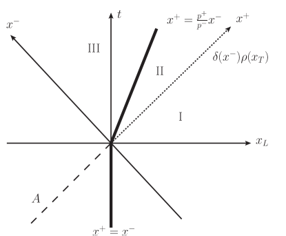
Figure 1: Longitudinal kinematics of the process. Nucleus A moving along the light cone with color current $\delta^{\mu+}\delta(x^{-})\rho(x_{T})$ meets with a stationary quark and is excited into a classical background Yang-Mills configuration $A^{\mu}=(0,0,A^{i}\,\,\theta(-x^{-}))$. In region I, for $x^{-}<0$, the background field is vacuum equivalent transverse field (26) and the fluctuation field $\delta A_{i}\equiv a_{i}$ is a gauge rotated Coulomb field of the stationary quark (56). In II and III there is no background field and the fluctuation field contains electrodynamics-like radiation caused by quark acceleration (67) and radiation from the quark-nucleus interaction (94).

III Field of an Isolated Particle and Wong’s Equations

The single particle is at rest before the collision. This is because the field strength $F^{\mu\nu}$ vanishes except in the thin sheet of colored glass. When it hits the Colored Glass it is accelerated, and begins to radiate. After the collision, it has a constant velocity to leading order in the strength of the small radiated field. We want to construct both the radiation field and the motion of the charged particle.

In the construction of the field of the charged particle, the extended current conservation law can cause a potential problem associated with the induced field of the classical particle rotating the current of the sheet of colored charge. We deal with this by working in the gauge for the small fluctuation field

$$\delta A^{-}\equiv a^{-}=0$$ (27)

In this gauge, combined with our choice for the gauge of the background field of the nucleus discussed above, the charges of both the nucleus and the single particle do not precess. This is since the only non-zero precession term is of order the single particle field times the source of the single particle field, and this is second order in the strength of the single particle field and we work only to first order. Note that one might be worried about some rotation induced while the charged particle traverses the sheet, but this occurs in a short time, and in our gauge, none of the fields diverge in the limit of infinitesimal sheet, and it therefore induces insignificant rotation.

So with these concepts in mind, let us now compute the trajectory of the single color charged particle as it traverses the sheet, determined by Wong’s equations wong ; wong2 . The classical particle in a colored field has a classical color vector $T_{a}(\tau)$, a trajectory $x^{\mu}(\tau)$ and momentum $p^{\mu}(\tau)$. Here $u^{\mu}=dx^{\mu}/d\tau$ and $p^{\mu}=mu^{\mu}$. The equation of motion is

$${{dp^{\mu}}\over{d\tau}}=gT\cdot F^{\mu\nu}u_{\nu}\equiv gT_{a}F^{\mu\nu}u_{\nu}.$$ (28)

Due to the asymmetry of $F^{\mu\nu}$ this explicitly conserves the square of the particle four-momentum $p$, i.e. $d(p_{\mu}p^{\mu})/d\tau=0$. By demanding covariant conservation $D^{\mu}J_{\mu}=0$ of the current

$$J_{\mu}(x)=\int d\tau\,T(\tau)u_{\mu}(\tau)\delta^{(4)}(x^{\mu}-x^{\mu}(\tau))$$ (29)

one sees that the equation for the precession of the colored charge matrix $T$ is

$${{dT}\over{d\tau}}=-ig[T,u\cdot A],$$ (30)

or, in component form

$${{dT_{a}}\over{d\tau}}=-gf_{abc}T^{c}A_{\mu}^{b}u^{\mu}.$$ (31)

A formal solution of this first-order matrix equation is the path ordered adjoint exponential

$$T(x)=P\exp\left(ig\int^{x}_{0}dx_{\mu}A^{\mu}\right)T(0),$$ (32)

where the path ordered integration over $x$ is over the trajectory of the particle.

Now before the collision, the integration above is entirely time-like, and the fields are 2-d transverse, so the integration over this part of the path vanishes, $dx_{i}A^{i}=0$. Near $x^{-}=0$, there is the integration across the sheet, but in our gauge the vector potential of the background field is so mildly singular, $A_{i}\sim\theta(-x^{-})$, that there is no contribution in the limit the sheet shrinks to zero. We ignore the contribution of the induced field produced by the single charged particle. Similarly, after the collision there is no contribution, since the background field from the nucleus vanishes there. Therefore, within the approximation of infinitely thin sheet we consider, the color of the particle does not precess.

Consider then the motion of the particle as given by Wong’s equations Eq. (28). Since in our gauge $F^{-i}=F^{-+}=0$, the simplest equation is the one with $\mu=-$:

$${dp^{-}\over d\tau}=0,$$ (33)

so that $p^{-}/m=u^{-}=dx^{-}/d\tau$ is a constant, $x^{-}(\tau)=u^{-}\tau$ and $\tau$ is effectively the same as $x^{-}$. Further, we have $F^{i+}=F_{-i}=\partial_{-}A^{i}$ and $u_{+}=-u^{-}$ so that the $\mu=i$ equation gives

$${dp^{i}\over d\tau}=u^{-}{dp^{i}\over dx^{-}}=-gT\cdot(\partial_{-}A^{i})u^{-}.$$ (34)

In this equation, the vector potential is evaluated at $x_{T}=0$, and since $T$ is the color charge at $x_{T}=0$, the overall result is gauge invariant. Before the sheet at $x^{-}<0$ $A^{i}$ is nonzero but effectively constant so that $p^{i}$ is constant. After the sheet at $x^{-}>0$ $A^{i}=0$ so that again $p^{i}$ is constant. Taking $p^{i}=0$ before the sheet and integrating Eq. (34) across $x^{-}=0$ gives the particle a kick of magnitude

$$p^{i}=-gT\cdot{\rm disc}A^{i}.$$ (35)

Finally, Wong’s equations explicitly conserve the mass shell condition $p^{2}=-m^{2}$ so that the $\mu=+$ equation simply enforces the mass shell condition.

We expect that the magnitude of the final transverse momentum into which the static quark is scattered is of the order of the relevant dynamical scale, the nuclear saturation momentum, $p_{i}p_{i}=p_{T}^{2}\sim Q_{\rm sat}^{2}$. A rough estimate could be $p_{T}^{2}\sim\langle\partial_{i}U\partial_{i}U^{\dagger}\rangle\sim Q_{\rm sat}^{2}\log(1/(\Lambda_{\rm QCD}r),$ where $r$ is the transverse separation of the two $U(x_{T})$ matrices and we used a standard formula ilm for the $UU^{\dagger}$ correlator. This expression diverges in the limit that we take the size of the particle probing our system to zero. This is an artifact of the high momentum divergence for average transverse momentum squared associated with the $1/p_{T}^{4}$ behavior of large angle scattering.

The current for the single particle may be computed from the constant trajectory $u^{\mu}=dx^{\mu}/d\tau=p^{\mu}/m$ and is for $x^{-}>0$ specified as

$$J^{\mu}(x) = T\int d\tau u^{\mu}\delta^{(4)}(x^{\mu}-u^{\mu}\tau)\,\theta(x^{-})$$ (36)

$$= Tu^{\mu}\int d\tau\delta(x^{-}-u^{-}\tau)\delta(x^{+}-u^{+}\tau)\delta^{(2)}(x^{i}-u^{i}\tau)\,\theta(x^{-})$$ (37)

$$= T{p^{\mu}\over p^{-}}\delta(x^{+}-{p^{+}\over p^{-}}x^{-})\delta^{(2)}(x^{i}-{p^{i}\over p^{-}}x^{-})\,\theta(x^{-}).$$ (38)

Notice that the delta function of involving $x^{-}$ simply sets the momentum space rapidity of the scattered particle equal to the coordinate space rapidity. In momentum space this current is

$$J^{\mu}(k)=\int d^{4}x\,e^{i(k^{+}x^{-}+k^{-}x^{+}-k^{i}x^{i})}J^{\mu}(x)={Tp^{\mu}\over i(p\cdot k-i\epsilon)}.$$ (39)

Similar expressions are valid for $x^{-}<0$; the sign of Eq. (39) as well as the sign of $\epsilon$ are then changed.

IV The Coulomb Potential in $\delta A^{-}=0$ Gauge

We have chosen the background color field of the nucleus to be of the form $A^{\mu}=(0,0,A^{i})$. In general, when discussing the total nucleus-quark system we will use the $A^{-}=0$ gauge. We will write the total field in the form $A^{\mu}+\delta A^{\mu}\equiv A^{\mu}+a^{\mu}$, where $\delta A^{\mu}=a^{\mu}$ is of lower order.

Before scattering off the sheet of colored class, the field of our classical particle is Coulombic. We have, with $r=\sqrt{x_{L}^{2}+x_{T}^{2}}=\sqrt{(x^{+}-x^{-})^{2}/2+x_{T}^{2}}$,

$$a^{\mu}_{Coul}={1\over{4\pi r}}\delta^{\mu 0},\qquad a^{+}=a^{-}={1\over{\sqrt{2}}}{1\over{4\pi r}},$$ (40)

where the matrix $gT$ that multiplies the charge has been suppressed. This field is shifted into the light cone gauge $a^{-}=0$ by an infinitesimal gauge transformation $U=e^{ig\Lambda}\approx 1+ig\Lambda$:

$$a^{\mu}\to a^{\mu}+D^{\mu}(A)\Lambda,\quad D^{\mu}=(\partial^{+},\partial^{-},\partial^{i}-igA^{i}),$$ (41)

or, in component form,

$$a^{-} \to {1\over{\sqrt{2}}}{1\over{4\pi r}}+\partial^{-}\Lambda=0,$$ (42)

$$a^{+} \to {1\over{\sqrt{2}}}{1\over{4\pi r}}+\partial^{+}\Lambda,$$ (43)

$$a^{i} \to 0+D^{i}\Lambda.$$ (44)

We are actually only concerned with this field for $x^{-}<0$, since the field for $x^{+}>0$ will include the radiation field and will be determined by solving a boundary value problem at $x^{-}=0$ with boundary conditions determined by the field for $x^{-}<0$.

The field $\Lambda$ (related to the infinitesimal transformation) is determined from Eq. (42):

$$\Lambda=-\int~{}dx^{-}{1\over{4\pi\sqrt{2}}}{1\over\sqrt{(x^{+}-x^{-})^{2}/2+x_{T}^{2}}}.$$ (45)

This gives

$$\Lambda={1\over{4\pi}}\ln{\left[\frac{1}{x_{T}}\left((x^{+}-x^{-})/\sqrt{2}+\sqrt{(x^{+}-x^{-})^{2}/2+x_{T}^{2}}\right)\right]}.$$ (46)

Note that $\partial^{-}\Lambda=-\partial_{+}\Lambda=\partial_{-}\Lambda$, where the first equality is general for LC coordinates, and the second holds since $\Lambda$ depends on the difference $x^{+}-x^{-}$. This yields for the $+$ component

$$a^{+}={\sqrt{2}\over{4\pi r}}.$$ (47)

Concerning the $i$ component, consider first the vacuum case so that $D_{i}=\partial_{i}$. Then

$$a^{i}=\partial_{i}\Lambda=-{1\over{4\pi}}{x^{i}\over x_{T}^{2}}{x_{L}\over r}={1\over\partial^{-}}{x^{i}\over 4\pi\sqrt{2}\,r^{3}}={1\over\partial_{+}}\partial^{i}{1\over 4\pi\sqrt{2}\,r}.$$ (48)

We have included some explicit relations which come in handy later. These fluctuation fields satisfy further

$$\partial_{+}a^{+}+\partial_{i}a^{i}=0,\quad\bigl{(}-2\partial_{+}\partial_{-}+\partial_{i}\partial_{i}\bigr{)}a^{i}=0,\quad\partial_{i}a_{j}-\partial_{j}a_{i}=0.$$ (49)

The last equation means that there is no longitudinal magnetic field.

One may ask whether there is residual gauge freedom in the transverse fields $a_{i}$. In fact, one can still do a U(1) gauge transformation ($C$ = constant)

$$a_{i}\to a_{i}+\partial_{i}\chi,\quad\chi=C\log x_{T},\quad\partial_{i}\chi=C{x_{i}\over x_{T}^{2}},\quad\partial_{T}^{2}\chi=0.$$ (50)

This transformation is the same as

$$\Lambda\to\Lambda+C\log x_{T}$$ (51)

and the 2-divergence of $a_{i}$ is invariant under it

$$\partial_{i}a^{i}={x_{L}\over 4\pi r^{3}}\to\partial_{i}(a^{i}+\partial_{i}\chi)=\partial_{i}a^{i}.$$ (52)

For the vacuum case, no nuclear background field, we now have the full set $a^{\mu}=(a^{+},0,a^{i})$. One can check that this form reproduces the desired structure for $F^{\mu\nu}$ as it must.

We will later need some Fourier transformations of the vacuum fields along the line $x^{-}=0$. To summarise:

$$\int_{-\infty}^{+\infty}dx^{+}d^{2}k_{T}\,e^{+i(k^{-}x^{+}-k^{i}x^{i})}{1\over 4\pi r}\biggl{(}1,{x^{i}\over r^{2}},{x_{L}x^{i}\over x_{T}^{2}}\biggr{)}={\sqrt{2}\over k_{T}^{2}+2(k^{-})^{2}}\biggl{(}1,ik^{i},-{k^{i}\over\sqrt{2}k^{-}}\biggr{)}.$$ (53)

V Field of test quark in a strong background field

For the non-abelian problem, one has to generalize the Coulomb solution to the case where for $x^{-}<0$ there is a strong background field $-igA_{i}=U\partial_{i}U^{\dagger}$, a two dimensional gauge transform of vacuum. Here $U$ is the gauge transformation matrix Eq. (25) transforming from the $A^{+}$ gauge to the $A^{i}$ gauge.

The fluctuation equation for the transverse field $a^{i}$ in the $A^{i}$ gauge is (see Eq. (84) below)

$$D_{\mu}D^{\mu}a^{i}=(-2\partial_{+}\partial_{-}+D_{i}D_{i})a^{i}=-2\partial_{+}\partial_{-}a^{i}+U\partial_{T}^{2}(U^{\dagger}a^{i})=Uj^{i},$$ (54)

where $j^{i}$ is a current representing a color source at $x_{L}=x_{T}=0$ in the $A^{+}$ gauge, in which there is no transverse background field. Multiplying from the left by $U^{\dagger}$ and noting that $\partial_{-}U=0$ (i.e.there is no $x^{+}$ dependence in the matrix $U$) shows that $U^{\dagger}a^{i}$ satisfies vacuum equations:

$$(-2\partial_{+}\partial_{-}+\partial_{T}^{2})U^{\dagger}a^{i}=j^{i},$$ (55)

i.e.,

$$a_{i}(x^{+},x^{-},x^{k})=U(x_{T})a_{i}^{\rm vac}(x^{+},x^{-},x^{k})\theta(-x^{-}).$$ (56)

In Eq. (56) $a_{i}^{\rm vac}$ satisfies the vacuum equations (see previous Section) and we inserted a theta function to remind that this discussion is relevant at $x^{-}<0$. The vacuum fields $a_{i}^{\rm vac}$ are determined with the color vector $T$ (sometimes $g$ is also appended) in the current.

One consequence of the appearance of $U$ in Eq. (56) is that the 2-divergence is modified by a coupling to the background field $A_{i}$:

$$\partial_{i}a_{i}=(\partial_{i}U(x_{T}))a_{i}^{\rm vac}+U\partial_{i}a_{i}^{\rm vac}=igA_{i}a_{i}+U(x_{T}){Tx_{L}\over 4\pi r^{3}},$$ (57)

where we inserted $\partial_{i}U=igA_{i}U$ and restored $T$. Also a longitudinal magnetic field is generated:

$$\epsilon_{Lij}\partial_{i}a_{j}=\epsilon_{ij}(\partial_{i}U)a_{j}^{\rm vac}=ig\epsilon_{ij}A_{i}a_{j}.$$ (58)

These equations are important since they give the first derivatives of the transverse radiation field, which are needed to solve the radiation equations, see Section VIII below. We also remind that the $a$th color component of the vector $igAa$ is $(igAa)_{a}=gf_{abc}A^{b}a^{c}$.

In a strong background field the Coulomb solution for $x^{-}<0$ is then

$$a^{0}_{Coul}={1\over{4\pi r}}U(x_{T})T.$$ (59)

We could redefine $T$ by an overall rotation to give

$$\overline{T}=U^{\dagger}(0)T$$ (60)

so that the Coulomb potential at $x_{T}=0$, where the quark is sitting, is $T/(4\pi r)$ without any rotation. However, the choice $U(0)=1$ is possible and will be made. The field in the gauge $a^{-}=0$ is as before obtained by a small gauge transformation with

$$\partial_{-}\Lambda=-{1\over\sqrt{2}\,4\pi r}U(x_{T})T$$ (61)

so that

$$a^{+}={1\over{\sqrt{2}}}a^{0}_{Coul}-\partial_{-}\Lambda=\sqrt{2}a_{Coul}^{0}$$ (62)

and

$$a^{i}=D^{i}\Lambda=U\partial_{i}(U^{\dagger}\Lambda)=-{1\over{\sqrt{2}}}D^{i}{1\over\partial^{-}}a_{Coul}^{0}=-{1\over{\sqrt{2}}}U{1\over\partial^{-}}\partial^{i}{T\over{4\pi r}}.$$ (63)

This, of course, is the same as Eq. (56), see also Eq. (48).

VI Radiation from a Point Particle Crossing a Sheet, QED and rapidity

In this section we review the computation of the radiation from a charged electromagnetic particle getting an impulse kick at $x^{-}=0$. This review will make the discussion of the non-abelian problem more transparent.

Let us assume we have a particle that is at rest at the origin for $t<0$ and is spontaneously accelerated to a particle with constant momentum $p^{\mu}$ at $t=0$. The current is

$$J^{\mu}=e\left[\delta^{\mu 0}\int_{-\infty}^{0}~{}d\tau\,\,\delta(t-\tau)\delta^{(3)}(\vec{x})+u^{\mu}\int_{0}^{\infty}~{}d\tau\,\,\delta^{(4)}(x^{\mu}-u^{\mu}\tau)\right].$$ (64)

Here $u^{\mu}=p^{\mu}/m$ is the four velocity of the particle after the collision. In light cone gauge $A^{-}=0$ the solution for the vector potential is

$$A^{+}={1\over\partial^{-}}(\nabla\cdot A+{1\over\partial^{-}}J^{-})$$ (65)

and

$$\partial_{\mu}\partial^{\mu}A^{i}=J^{i}-{\partial^{i}\over\partial^{-}}J^{-}.$$ (66)

If we rewrite this in Fourier space, then the distribution of radiation is

$$16\pi^{3}k{{dN}\over{d^{3}k}}=\lim_{k^{2}\rightarrow 0}~{}k^{4}A^{i}(k)A^{i}(-k)=\left[J^{i}(k)-{k^{i}\over k^{-}}J^{-}(k)\right]\left[J^{i}(-k)-{k^{i}\over k^{-}}J^{-}(-k)\right].$$ (67)

In the following, we will assume $k^{2}=0$. Up to a term that vanishes when $k^{2}=0$, upon use of current conservation $k\cdot J=0$, the right hand side is algebraically identical to

$$16\pi^{3}k{{dN}\over{d^{3}k}}=J_{\mu}(k)J^{\mu}(-k)$$ (68)

which is the ordinary text book expression.

We can now compute the Fourier transform of the current as

$$J^{\mu}=e\left[\delta^{\mu 0}{1\over{ik^{0}}}-u^{\mu}{1\over(ik\cdot u)}\right].$$ (69)

After a little algebra, we find that

$$J^{2}=e^{2}v^{2}{1\over k^{2}}{{\sin^{2}\theta}\over{(1-v\cos\theta)^{2}}},$$ (70)

where the angle $\theta$ is between that of the 3-dimensional velocity vector ${\bf v}={\bf p}/E$ of the particle and the emitted photon $(k=|{\bf k}|=\omega)$.

Although we are mainly interested in a stationary initial quark, it may be useful to give some expressions for a more general radiation process with momenta $q\to k+p$ and write them in terms of rapidities,

$$k^{\mu}=k_{T}({\textstyle{{1\over\sqrt{2}}}}e^{y},{\textstyle{{1\over\sqrt{2}}}}e^{-y},\cos\phi,\sin\phi),\quad q^{\mu}=({\textstyle{{m_{Tq}\over\sqrt{2}}}}e^{y_{q}},{\textstyle{{m_{Tq}\over\sqrt{2}}}}e^{-y_{q}},q_{T}\cos\phi_{q},q_{T}\sin\phi_{q}),$$ (71)

where $m_{Tq}^{2}=m^{2}+q_{T}^{2}$, and similarly for $p^{\mu}$. The radiation current in Eqs. (39,69) for instantaneous acceleration $q\to p$ at $x^{-}=0$ is

$$J^{\mu}(k)=+iT\biggl{(}{q^{\mu}\over q\cdot k}-{p^{\mu}\over p\cdot k}\biggr{)}.$$ (72)

Using the kinematic relation $|k^{i}-k^{-}p^{i}/p^{-}|^{2}=-2(k^{-}/p^{-})\,p\cdot k$ this gives

$$-k^{2}A_{i}(k)=J^{i}(k)-{k^{i}\over k^{-}}J^{-}(k)=2iT\left[{k^{i}-{k^{-}\over q^{-}}q^{i}\over|k^{i}-{k^{-}\over q^{-}}q^{i}|^{2}}-{k^{i}-{k^{-}\over p^{-}}p^{i}\over|k^{i}-{k^{-}\over p^{-}}p^{i}|^{2}}\right],$$ (73)

where the first term corresponds to $\theta(-x^{-})$ and the second to $\theta(x^{-})$. The ratio $k^{-}/p^{-}$ is the fractional light cone energy taken by the photon from the emitting charge. The multiplicity can now be computed from Eq. (67) or Eq. (68). For a massless quark one has

$${dN\over dyd^{2}k_{T}}={g^{2}T_{a}T_{a}\over(2\pi)^{3}}\,{1\over k_{T}^{2}}{\cosh(y_{p}-y_{q})-\cos(\phi_{p}-\phi_{q})\over(\cosh(y-y_{q})-\cos(\phi-\phi_{q}))(\cosh(y-y_{p})-\cos(\phi-\phi_{p}))}.$$ (74)

Integration over the azimuthal angle of the produced gluon produces $dN/dydk_{T}^{2}$. This can also be done analytically using

$$\int_{0}^{2\pi}{d\phi\over(\cosh y_{1}-\cos(\phi-\phi_{1})(\cosh y_{2}-\cos(\phi-\phi_{2})}={2\pi(\coth y_{1}+\coth y_{2})\over\cosh(y_{1}+y_{2})-\cos(\phi_{1}-\phi_{2})}.$$ (75)

Initial static quark, the case were interested in, is obtained from the general formulas in the limit of large mass, $m\gg q_{T},\,p_{T}$ and $y_{q}=0$. If the static quark is accelerated into rapidity $y_{p}$, the gluon distribution is

$${dN\over dyd^{2}k_{T}}={g^{2}T_{a}T_{a}\over(2\pi)^{3}}\,{1\over 2k_{T}^{2}}\biggl{(}{\sinh(y_{p})\over\cosh(y-y_{p})\cosh(y)}\biggr{)}^{2}.$$ (76)

The distribution, plotted in Fig. 2 is symmetric around $y=y_{p}/2$ and has a broad plateau around the maximum. The maximum value is $4\tanh^{2}{y_{p}\over 2}$ and the value at $y=0$ or $y=y_{p}$ is $\tanh^{2}y_{p}$. For large $y_{p}$ and small $y$, in the “target fragmentation region”, the distribution grows like

$$\biggl{(}{2\over 1+e^{-2y}}\biggr{)}^{2}.$$ (77)

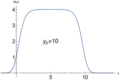
Figure 2: Rapidity distribution (bracketed factor in Eq. (76) is plotted) of gluons emitted in an acceleration of a static quark to rapidity $y_{p}=10$ by the nucleus. The maximum is at $y_{p}/2=5$ and the curve is symmetri around the maximum value.

VII Boundary Conditions

We have now discussed the transverse fluctuation field $a_{i}$ at $x^{-}>0$ before the arrival of the nucleus as well as the classical radiation from the acceleration of the quark. What is missing is $a_{i}$ after the nucleus has passed. However, we have fixed the gauge so that there is no background field at $x^{-}>0$. The solution thus is a free plane wave and one only needs the boundary conditions at $x^{-}=0$.

Actually we already know the boundary condition for $a_{i}$ when approaching from the direction of $x^{-}<0$; according to Eq. (56) the value on the surface $x^{-}=0$ is

$$a_{i}^{S}(x^{+},x^{k})\equiv a_{i}(x^{+},x^{-}=0,x^{k})=U(x_{T})a_{i}^{\rm vac}(x^{+},x^{-}=0,x^{k}).$$ (78)

But are there discontinuities on the nuclear sheet at $x^{-}=0$? By studying fluctuation equations we shall show that there is a discontinuity in $a^{+}$ but not in $a^{-}$ or $a^{i}$.

The equation for the small fluctuation field is

$$D^{2}a^{\mu}-D^{\mu}(D\cdot a)-2igF^{\mu\nu}a_{\nu}=Uj^{\mu}.$$ (79)

The only place where one might generate a discontinuity of the field $a$ is when a derivative with respect to $x^{-}$ multiplies a field $A^{i}$. This only occurs in the plus component of the equation of motion:

$$D^{2}a^{+}-D^{+}(D\cdot a)-2igF^{+i}a_{i}=Uj^{+},$$ (80)

which can be rewritten as

$$U\partial^{2}_{T}(U^{\dagger}a^{+})+\partial_{-}\left(-\partial_{+}a^{+}+D_{i}a^{i}+2igA^{i}a_{i}\right)-2igA^{i}\partial_{-}a^{i}=Uj^{+}.$$ (81)

Collecting all the terms containing $\partial_{-}$ in the $+$ equation one sees that they are

$$\partial_{-}(-\partial_{+}a^{+}+D_{i}a^{i}+2igA^{i}a_{i})-2igA^{i}\partial_{-}a^{i}.$$ (82)

The discontinuity in $D_{i}a^{i}$ combines with that in the next term and any discontinuity in $A^{i}$ can be cancelled by a discontinuity in $\partial_{+}a^{+}$:

$${\rm disc}\,\partial_{+}a^{+}=ig~{}{\rm disc}(A^{i})a_{i}.$$ (83)

In the $i$ component, there is no such term (in the gauge $a^{-}=0$ in which we work). This equation forces $a^{i}$ to be continuous.

The radiation may be computed by knowing the asymptotic behaviour of the field $a^{i}$, which satisfies the fluctuation equation

$$D^{2}a^{i}-D^{i}(D\cdot a)=Uj^{i}.$$ (84)

For $x^{-}>0$, where the matrix $U=1$, this equation simplifies to

$$\partial^{2}a^{i}-\partial^{i}(D\cdot a)=j^{i}.$$ (85)

Further, using the equation for the minus component of the current,

$$\partial^{-}(D\cdot a)=-j^{-}$$ (86)

we find that for $x^{-}>0$ the equation for $a_{i}$ simply is

$$\partial^{2}a^{i}=j^{i}-\partial^{i}\frac{1}{\partial^{-}}j^{-}.$$ (87)

VIII Radiation from the quark-nucleus interaction

The transverse radiation field is

$$a_{i}(x^{+},x^{-},x^{j})=\int{d^{4}k\over(2\pi)^{4}}e^{-i(k^{+}x^{-}+k^{-}x^{+}-k_{j}x_{j})}\,\,a_{i}(k^{-},k^{+},k^{j})$$ (88)

and radiation is computed from $k^{2}a_{i}(k^{-},k^{+},k^{j})$. We know that $a_{i}$ is a free field at $x^{-}>0$ and further we know its boundary value Eq. (78) at $x^{-}=0$. With this information we can construct the full solution.

First, from the fact that one has a free solution for $x^{-}>0$ one can conclude that

$$a_{i}(k^{-},k^{+},k^{j})={i\over k^{+}-{k_{T}^{2}\over 2k^{-}}+i\epsilon}a_{i}(k^{-},k^{j})={-2ik^{-}\over k^{2}+i\epsilon}a_{i}(k^{-},k^{j}).$$ (89)

Inserting this to Eq. (88) gives

$$a_{i}(k^{-},x^{-},k^{j})=\theta(x^{-})\exp(-i{k_{T}^{2}\over 2k^{-}}x^{-})a_{i}(k^{-},k^{j}),$$ (90)

where $a_{i}(k^{-},k^{j})$ is the Fourier transform of the boundary value $U(x_{T})a_{i}^{\rm vac}(x^{+},0,x^{j})$ in Eq. (78)

$$a_{i}(k^{-},k^{j}) = \int dx^{+}d^{2}xe^{i(k^{-}x^{+}-k^{j}x^{j})}\,U(x^{j})\,a_{i}^{\rm vac}(x^{+},0,x^{j})$$ (91)

$$= \int{d^{2}q\over(2\pi)^{2}}U(k_{j}-q_{j}){-q_{i}\over k^{-}(q_{T}^{2}+2(k^{-})^{2})}.$$ (92)

The Fourier transformation was taken from Eq. (53). From Eq. (89)

$$ik^{2}a_{i}(k^{-},k^{+},k^{j})=2k^{-}a_{i}(k^{-},k^{j}).$$ (93)

Radiation from the quark-sheet collision is then computed from (color vector $T$ is now explicitly written)

$$16\pi^{3}{{dN}\over{dyd^{2}k}}=\left\langle\left|\int{d^{2}q\over(2\pi)^{2}}U(k_{j}-q_{j})T{2q^{i}\over q_{T}^{2}+2(k^{-})^{2}}\right|^{2}\right\rangle_{\rho},$$ (94)

which, together with radiation from acceleration of the quark, is the main result of this article. For quantitative evaluation one firstly has to compute the convolution in Eq. (94) and then perform the quantum average over an ensemble of color distributions.

The computation of the convolution and color ensemble averaging is a challenging task and we shall here only show how the result approaches the Gunion-Bertsch formula gb ; kmw for small $p_{T}$ particle production in the central region.

Note first that Eq. (92) contains part of the ED-like radiation solution discussed in Section VI. To avoid double counting, this should be eliminated. To this end, write

$$a^{i}=\beta^{i}_{1}+\beta^{i}_{2}.$$ (95)

We let $\beta_{1}$ be the solution to the free equations of motion in the presence of the current, that is the analog of the electrodynamics problem for all $x^{-}$:

$$\partial_{\mu}\partial^{\mu}\,\beta^{i}_{1}=j^{i}-{{\partial^{i}}\over\partial^{-}}j^{-},$$ (96)

where the current is Eq. (64) with $e$ replaced by the unrotated color vector $T$. The solution is precisely the solution Eq. (69) to the electrodynamics problem of radiation from a charged particle.

We let $\beta_{2}$ be the solution of the free zero external current wave equation $\partial_{\mu}\partial^{\mu}\,\beta^{i}_{2}=0$ subject to the boundary condition

$$\beta^{i}_{2}\mid_{x^{-}=0}=Ua_{i}^{\rm vac}\mid_{x^{-}=0}-\beta^{i}_{1}\mid_{x^{-}=0}=Ua_{i}^{\rm vac}\mid_{x^{-}=0}-a_{i}^{\rm vac}\mid_{x^{-}=0}$$ (97)

This solution for $x^{-}>0$ will satisfy correct equations of motion with the proper boundary conditions at $x^{-}=0$. Here one has subtracted the contribution of $\beta^{i}_{1}$ at the surface $x^{-}=0$ which is simply the Coulomb solution at $x^{-}=0$, $a_{i}^{\rm vac}$, the solution with unrotated charge vector $T$.

To compute the convolution Eq. (92) we construct a derivative or momentum expansion as follows. Write the boundary or surface value in the form

$$a_{i}^{S}=a_{i}(x^{+},x^{-}=0,x^{j})=U(x_{T})a_{i}^{\rm vac}(x^{+},x^{-}=0,x^{j})=\partial_{i}\eta+\epsilon_{ij}\partial_{j}\chi.$$ (98)

The two functions $\eta,\chi$ can be projected out ($\epsilon_{12}=-\epsilon_{21}=1$)

$$\partial_{T}^{2}\eta=\delta_{ir}\partial_{r}a_{i}=\partial_{i}a_{i}^{S},\quad\partial_{T}^{2}\chi=\epsilon_{ir}\partial_{r}a_{i}^{S}.$$ (99)

Solving $\eta,\chi$ from here and inserting back to Eq. (98) gives the indentity

$$a_{i}^{S}=(\delta_{ij}\delta_{sr}+\epsilon_{ij}\epsilon_{sr}){1\over\partial_{T}^{2}}\partial_{j}\partial_{r}a_{s}^{S}.$$ (100)

In the last term one can write

$$\partial_{r}a_{s}^{S} = \partial_{r}U\,a_{s}^{\rm vac}+U\partial_{r}a_{s}^{\rm vac}$$ (101)

$$= igA_{r}Ua_{s}^{\rm vac}+U\partial_{r}a_{s}^{\rm vac}$$

$$= igA_{r}a_{s}^{\rm vac}+\partial_{r}a_{s}^{\rm vac}+{\cal O}(U-1).$$

Inserting this back to Eq. (100) gives the approximation

$$a_{i}^{S}=(\delta_{ij}\delta_{sr}+\epsilon_{ij}\epsilon_{sr}){1\over\partial_{T}^{2}}\partial_{j}(igA_{r}a_{s}^{\rm vac})+a_{i}^{\rm vac}.$$ (102)

The last term just goes through Eq. (100) unchanged, but disappears when the inhomogeneous solution is subtracted as in Eq. (97). In Fourier space we thus have

$$ik^{2}a_{i}^{S}=(\delta_{ij}\delta_{sr}+\epsilon_{ij}\epsilon_{sr})gf_{abc}{k_{j}\over k_{T}^{2}}\int{d^{2}q\over(2\pi)^{2}}A_{r}^{b}(k_{m}-q_{m})a_{s}^{c}(k^{-},q_{m})2k^{-}.$$ (103)

Squaring this and summing over $i$ involves the tensorial structure

$$\sum_{i=1}^{2}(\delta_{ij}\delta_{sr}+\epsilon_{ij}\epsilon_{sr})k_{j}A_{r}a_{s}(\delta_{i\alpha}\delta_{\beta\gamma}+\epsilon_{i\alpha}\epsilon_{\beta\gamma})k_{\alpha}A_{\beta}a_{\gamma}=k_{T}^{2}A_{T}^{2}a_{T}^{2}$$ (104)

so that

$${dN\over dyd^{2}k_{T}}={g^{2}\over 16\pi^{3}}f_{abc}f_{a{\hat{b}}{\hat{c}}}{1\over k_{T}^{2}}\int{d^{2}q_{1}d^{2}q_{2}\over(2\pi)^{4}}A_{r}^{b}(k^{i}-q_{1}^{i})A_{r}^{\hat{b}}(k^{i}-q_{2}^{i})a^{c}_{s}a^{\hat{c}}_{s}(k^{-},q_{2}^{i})(2k^{-})^{2}.$$ (105)

To proceed further one must go beyond the classical approximation by introducing quantum expectation values ilm of the background field correlator

$$\langle A_{i}^{a}(k_{1})A_{j}^{b}(k_{2})\rangle=\delta_{ab}(2\pi)^{2}\delta^{(2)}(k_{1}-k_{2})g^{2}\mu^{2}{k_{1}^{i}k_{2}^{j}\over k_{1T}^{2}k_{2T}^{2}}.$$ (106)

Fourier transformations of $a_{i}^{\rm vac}$ along the line $x^{-}=0$ were listed in Eq. (53). The relevant one is

$$2k^{-}a_{i}^{\rm vac}(k^{-},q^{j})={-2q^{i}\over q_{T}^{2}+2(k^{-})^{2}},$$ (107)

the extra factor $k^{-}$, which arose from constructing $k^{2}$, cancels. For the color factors one can write $f_{abc}f_{ab{\hat{c}}}T_{c}T_{\hat{c}}=N_{c}T_{\hat{c}}T_{\hat{c}}=N_{c}N_{g}$. With these simplifications Eq. (105) reduces to the form

$${dN\over dyd^{2}k_{T}}={g^{4}\mu^{2}\over 16\pi^{3}}N_{c}N_{g}{1\over k_{T}^{2}}\int{d^{2}q\over(2\pi)^{2}}{1\over|k^{i}-q^{i}|^{2}}{q_{T}^{2}\over(q_{T}^{2}+2(k^{-})^{2})^{2}}.$$ (108)

If $y$ is the gluon rapidity, $2(k^{-})^{2}=k_{T}^{2}e^{-2y}$. At large $y$ away from the fragmentation region at $y=0$ this vanishes and the momentum integral in Eq. (108) approaches the standard GB form

$${1\over k_{T}^{2}}\int{d^{2}q\over(2\pi)^{2}}{1\over|k^{i}-q^{i}|^{2}}{1\over q_{T}^{2}}.$$ (109)

Consider then including the last term $a_{i}^{\rm vac}$ in Eq. (102), which was subtracted as part of the inhomogeneous solution. Due to the antisymmetric tensor $f_{abc}$ in the first term, upon squaring the interference term anyway vanishes. The square of this term gives the gluon distribution

$${dN\over dyd^{2}k_{T}}={g^{2}\over 16\pi^{3}}T_{a}T_{a}{4k_{T}^{2}\over(k_{T}^{2}+2(k^{-})^{2})^{2}}={g^{2}\over 16\pi^{3}}T_{a}T_{a}{1\over k_{T}^{2}}\biggl{(}{2\over 1+e^{-2y}}\biggr{)}^{2}.$$ (110)

This is precisely the fragmentation region radiation in the limit of large quark mass, computed in Eq. (77).

Our final result for gluon production is obtained by taking $ik^{2}a_{i}$ from Eqs. (92,93) for the homogeneous $\beta_{2}$ contribution (quark-sheet collision) and from Eq. (73) for the inhomogeneous $\beta_{1}$ contribution (quark acceleration), summing and absolute squaring. In the above discussion, we have ignored the contribution for a possible interference term. This term vanishes. This follows because the color structure of the sum is $UT+T$ so that the interference is $\sim UT\cdot T$. Taking ensemble average over $\rho$ distribution leads to $\langle U\rangle=0$ and interference vanishes. In the weak field approximation Eq. (103) the interference term is $\sim f_{abc}T_{a}T_{c}=0$ and vanishes on tree level. Gluon production therefore arises from two non-interfering contributions: one that is the generalization of the QED radiation process (type $\beta_{1}$) and another which is unique to QCD, and arises from the disturbance of a Coulomb field composed of colored gluons that is disturbed during the collision process (type $\beta_{2}$)

IX Rapidity and $k_{T}$ distribution

Our goal is to study the fragmentation region so we are interested in the rapidity dependence of the produced radiation. The ED-like radiation from the acceleration of the quark when crossing the nuclear sheet was studied in Section VI, see Fig. 2 for distribution at fixed $k_{T}$ and fixed acceleration. This is the inhomogeneous solution of the radiation equation and depends on the path of the accelerated quark. The homogeneous solution depends on the color charge distribution of the sheet colliding with the quark and in Eq. (108). Its rapidity dependence is built in $2(k^{-})^{2}=k_{T}^{2}e^{-2y}$. To see what it is quantitatively, we have to introduce an IR divergence regulator mass $m$ in the momentum integral in Eq. (108). It can then be written in the form

$${1\over k_{T}^{2}}\int{d^{2}q\over(2\pi)^{2}}{1\over|k^{i}-q^{i}|^{2}+m^{2}}{q^{2}\over(q^{2}+m^{2}+k_{T}^{2}e^{-2y})^{2}}$$ (111)

$$={1\over 4\pi k_{T}^{4}}\int_{0}^{\infty}du{u\over(u+\hat{M}^{2})^{2}}{1\over\sqrt{(1-u)^{2}+2\hat{m}^{2}(1+u)+\hat{m}^{4}}}$$

$$={1\over 2\pi k_{T}^{4}}\biggl{[}\log{k_{T}\over m\sqrt{m^{2}/k_{T}^{2}+e^{-2y}}}-{1\over 2}+{\cal O}\biggl{(}{m^{2}\over k_{T}^{2}}\biggr{)}\biggr{]},$$ (112)

where $\hat{M}^{2}=m^{2}/k_{T}^{2}+e^{-2y}$, $\hat{m}=m/k_{T}$. The integral can be done in closed form and expressed rather compactly by introducing $v^{2}=1+2\hat{m}^{2}+2\hat{M}^{2}+(\hat{M}^{2}-\hat{m}^{2})^{2}$. What is relevant is the limit $m\ll k_{T}$ shown in Eq. (112). The result has the characteristic features:

• The $k_{T}$ distribution of the quark-sheet collision goes like $\log(k_{T})/k_{T}^{4}$ while that from the quark acceleration goes like $1/k_{T}^{2}$. Different variation in different ranges of $k_{T}$ is discussed, for example, in dumitru .

• The rapidity distribution of the quark-sheet collision includes a target fragmentation region for $y<\log(k_{T}/m)$, $m=$ IR regulator, within which the distribution shows a linear increase, Fig. 3, beyond which there is a plateau extending arbitrarily. The distribution following from quark acceleration has a natural large $y$ cut-off given by the momentum of the accelerated quark.

At first sight, the different $k_{T}$ dependences of these two processes seems alarming. It should not be so. The $k_{T}$ dependence of $1/k_{T}^{2}$ is only valid for the direct charged particle emission and in the range where $k_{T}\ll Q_{\rm sat}^{\rm proj}$, that is when the typical transverse momentum of the emitted gluon is small compared to the typical momentum kick the charged particle gets from scattering from the nucleus. At higher momentum, we simply must modify the computation to take into account the charged particle recoil. In this region the production cross section will fall like $1/k_{T}^{4}$, although our method of computation presented here will fail in this region.

For the Gunion-Bertsch contribution, we explicitly worked in the region where $k_{T}\gg Q_{\rm sat}^{\rm proj}$. In this region the non-linearities of the projectile color field are unimportant. Our approximations are valid in this region since no large recoil of the charged particle is required, and this region provides a useful check of our computations.

The interesting region of computation is when the $Q_{\rm sat}^{\rm targ}\ll k_{T}\ll Q_{\rm sat}^{\rm proj}$. This is where most of the particle production takes place. In this region, the Gunion-Bertsch computation is not sufficient, and the full non-linearity of the projectile color field must be properly taken into account, i.e., a more accurate evaluation of the expectation value in Eq. (94) is needed.

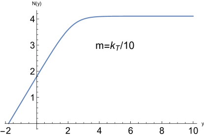
Figure 3: Rapidity distribution (bracketed factor in Eq. (112) is plotted) at fixed $k_{T}$ of gluons emitted in a collision of an initially static quark with nucleus. The IR regulator mass is $k_{T}/10$ and the curve shows a linear increase as a function of rapidity in the fragmentation region.

X Conclusions

We have in this article computed gluon production in a collision of an ultrarelativistic nucleus and a static quark. The result consists of two parts, an ED-like inhomogeneous contribution from quark acceleration (Eqs. (67,73) and a homogeneous contribution from the interaction between the nuclear sheet and the quark (Eq. (94)). This interaction term corresponded to a homogeneous solution of the radiation equation due to a special gauge choice (25) in which the gauge field vanished after the passage of the sheet.

This is only the first step towards the final goal, making predictions for target fragmentation dynamics of ultrarelativistic nuclear collisions. The next step involves performing the transverse momentum convolution and the color ensemble averaging in Eq. (94). Here they were carried out only for dilute systems. Next these gluonic results should be combined with those for quarks in McLerran:2018avb to give initial values for energy-momentum and baryon number. This is analogous with the very early work in km . Finally, one should numerically go through hydrodynamic evolution in analogy with Kajantie:1982zb and prepare predictions for experiments - which hopefully some day will well extend to the fragmentation region.

- (1) R. Anishetty, P. Koehler and L. D. McLerran, “Central Collisions Between Heavy Nuclei at Extremely High-Energies: The Fragmentation Region,” Phys. Rev. D 22 (1980) 2793. doi:10.1103/PhysRevD.22.2793
- (2) K. Kajantie and L. D. McLerran, “Energy Densities, Initial Conditions and Hydrodynamic Equations for Ultrarelativistic Nucleus-nucleus Collisions,” Nucl. Phys. B 214, 261 (1983). doi:10.1016/0550-3213(83)90662-4
- (3) L. McLerran, “From the Glasma to the QCD Phase Boundary,” Acta Phys. Polon. Supp. 10, 663 (2017) doi:10.5506/APhysPolBSupp.10.663 [arXiv:1612.00864 [hep-ph]].
- (4) L. McLerran, “The Fragmentation Region of High Energy Nucleus-Nucleus and Hadron-Nucleus Collisions,” EPJ Web Conf. 172 (2018) 03003. doi:10.1051/epjconf/201817203003
- (5) L. D. McLerran and R. Venugopalan, “Gluon distribution functions for very large nuclei at small transverse momentum,” Phys. Rev. D 49, 3352 (1994) doi:10.1103/PhysRevD.49.3352 [hep-ph/9311205].
- (6) A. H. Mueller and J. w. Qiu, “Gluon Recombination and Shadowing at Small Values of x,” Nucl. Phys. B 268 (1986) 427. doi:10.1016/0550-3213(86)90164-1
- (7) L. V. Gribov, E. M. Levin and M. G. Ryskin, “Semihard Processes in QCD,” Phys. Rept. 100 (1983) 1. doi:10.1016/0370-1573(83)90022-4
- (8) A. H. Mueller, “Small x Behavior and Parton Saturation: A QCD Model,” Nucl. Phys. B 335 (1990) 115. doi:10.1016/0550-3213(90)90173-B
- (9) L. D. McLerran, S. Schlichting and S. Sen, “Space-Time Picture of Baryon Stopping in the Color-Glass Condensate,” arXiv:1811.04089 [hep-ph].
- (10) A. Kovner, L. D. McLerran and H. Weigert, “Gluon production at high transverse momentum in the McLerran-Venugopalan model of nuclear structure functions,” Phys. Rev. D 52, 3809 (1995) doi:10.1103/PhysRevD.52.3809 [hep-ph/9505320].
- (11) Y. V. Kovchegov and A. H. Mueller, “Gluon production in current nucleus and nucleon - nucleus collisions in a quasiclassical approximation,” Nucl. Phys. B 529 (1998) 451 doi:10.1016/S0550-3213(98)00384-8 [hep-ph/9802440].
- (12) A. Dumitru and L. D. McLerran, “How protons shatter colored glass,” Nucl. Phys. A 700, 492 (2002) doi:10.1016/S0375-9474(01)01301-X [hep-ph/0105268].
- (13) A. Krasnitz, Y. Nara and R. Venugopalan, “Coherent gluon production in very high-energy heavy ion collisions,” Phys. Rev. Lett. 87, 192302 (2001) doi:10.1103/PhysRevLett.87.192302 [hep-ph/0108092].
- (14) T. Lappi, “Production of gluons in the classical field model for heavy ion collisions,” Phys. Rev. C 67, 054903 (2003) doi:10.1103/PhysRevC.67.054903 [hep-ph/0303076].
- (15) J. P. Blaizot, F. Gelis and R. Venugopalan, “High-energy pA collisions in the color glass condensate approach. 1. Gluon production and the Cronin effect,” Nucl. Phys. A 743, 13 (2004) doi:10.1016/j.nuclphysa.2004.07.005 [hep-ph/0402256].
- (16) F. Gelis and Y. Mehtar-Tani, “Gluon propagation inside a high-energy nucleus,” Phys. Rev. D 73, 034019 (2006) doi:10.1103/PhysRevD.73.034019 [hep-ph/0512079].
- (17) F. Gelis, A. M. Stasto and R. Venugopalan, “Limiting fragmentation in hadron-hadron collisions at high energies,” Eur. Phys. J. C 48, 489 (2006) doi:10.1140/epjc/s10052-006-0020-x [hep-ph/0605087].
- (18) E. Iancu, C. Marquet and G. Soyez, “Forward gluon production in hadron-hadron scattering with Pomeron loops,” Nucl. Phys. A 780, 52 (2006) doi:10.1016/j.nuclphysa.2006.08.017 [hep-ph/0605174].
- (19) J. Casalderrey-Solana and E. Iancu, “Interference effects in medium-induced gluon radiation,” JHEP 1108, 015 (2011) doi:10.1007/JHEP08(2011)015 [arXiv:1105.1760 [hep-ph]].
- (20) Y. Mehtar-Tani, C. A. Salgado and K. Tywoniuk, JHEP 1204, 064 (2012) doi:10.1007/JHEP04(2012)064 [arXiv:1112.5031 [hep-ph]].
- (21) N. Armesto, H. Ma, M. Martinez, Y. Mehtar-Tani and C. A. Salgado, “Interference between initial and final state radiation in a QCD medium,” Phys. Lett. B 717, 280 (2012) doi:10.1016/j.physletb.2012.09.039 [arXiv:1207.0984 [hep-ph]].
- (22) N. Armesto, H. Ma, M. Martinez, Y. Mehtar-Tani and C. A. Salgado, “Coherence Phenomena between Initial and Final State Radiation in a Dense QCD Medium,” JHEP 1312, 052 (2013) doi:10.1007/JHEP12(2013)052 [arXiv:1308.2186 [hep-ph]].
- (23) E. Iancu, A. Leonidov and L. McLerran, “The Color glass condensate: An Introduction,” hep-ph/0202270.
- (24) F. Gelis and R. Venugopalan, “Three lectures on multi-particle production in the glasma,” Acta Phys. Polon. B 37, 3253 (2006) [hep-ph/0611157].
- (25) S. K. Wong, “Field and particle equations for the classical Yang-Mills field and particles with isotopic spin,” Nuovo Cim. A 65, 689 (1970). doi:10.1007/BF02892134
- (26) J. Jalilian-Marian, S. Jeon and R. Venugopalan, “Wong’s equations and the small x effective action in QCD,” Phys. Rev. D 63, 036004 (2001) doi:10.1103/PhysRevD.63.036004 [hep-ph/0003070].
- (27) J. F. Gunion and G. Bertsch, “Hadronization By Color Bremsstrahlung,” Phys. Rev. D 25, 746 (1982). doi:10.1103/PhysRevD.25.746
- (28) K. Kajantie and R. Raitio, “Quark Gluon Plasma in Ultrarelativistic Nucleus-nucleus Collisions,” Phys. Lett. 121B, 415 (1983). doi:10.1016/0370-2693(83)91189-9