A sequence of polynomials with optimal condition number

Abstract.

We find an explicit sequence of univariate polynomials of arbitrary degree with optimal condition number. This solves a problem posed by Michael Shub and Stephen Smale in 1993.

1. Introduction

1.1. The Weyl norm and the condition number of polynomials

Closely following the notation of the celebrated paper [BezIII], we denote by $\ \mathcal{H}_{N}$ the vector space of bivariate homogeneous polynomials of degree $N$, that is the set of polynomials of the form

(1) $$g(x,y)=\sum_{i=0}^{N}a_{i}x^{i}y^{N-i},\quad a_{i}\in\mathbb{C}$$

where $x,y$ are complex variables. The Weyl norm of $g$ (sometimes called Kostlan or Bombieri-Weyl or Bombieri norm) is

$$\|g\|=\left(\sum_{i=0}^{N}\binom{N}{i}^{-1}|a_{i}|^{2}\right)^{1/2},$$

where the binomial coefficients in this definition are introduced to satisfy the property $\|g\|=\|g\circ U\|$ where $U\subseteq\mathbb{C}^{2\times 2}$ is any unitary $2\times 2$ matrix and $g\circ U\in\ \mathcal{H}_{N}$ is the polynomial given by $g\circ U(x,y)=g(U\binom{x}{y})$. Indeed, with this metric we have

$$\|g\|^{2}=\frac{N+1}{\pi}\int_{\mathbb{P}(\mathbb{C}^{2})}\frac{|g(\eta)|^{2}}{\|\eta\|^{2N}}\,dV(\eta),$$

where the integration is made with respect to volume form $V$ arising from the standard Riemannian structure in $\mathbb{P}(\mathbb{C}^{2})$. Note that the expression inside the integral is well defined since it does not depend on the choice of the representative of $\eta\in\mathbb{P}(\mathbb{C}^{2})$.

The zeros of $g$ lie naturally in the complex projective space $\mathbb{P}(\mathbb{C}^{2})$. The condition number of $g$ at a zero $\zeta$ is defined as follows. If the derivative $Dg(\zeta)$ does not vanish, by the Implicit Function Theorem the zero $\zeta$ of $g$ can be continued in a unique differentiable manner to a zero $\zeta^{\prime}$ of any sufficiently close polynomial $g^{\prime}$. This thus defines (locally) a solution map given by $Sol(g^{\prime})=\zeta^{\prime}$. The condition number is by definition the operator norm of the derivative of the solution map, in other words $\mu(g,\zeta)=\|DSol(g,\zeta)\|$, where the tangent spaces $T_{g}\ \mathcal{H}_{N}$ and $T_{\zeta}\mathbb{P}(\mathbb{C}^{2})$ are endowed respectively with the Bombieri–Weyl norm and the Fubini–Study metric. In [BezI] it was proved that

(2) $$\mu(g,\zeta)=\|g\|\,\|\zeta\|^{N-1}|(Dg(\zeta)\mid_{\zeta^{\perp}})^{-1}|,$$

(the definition and theory in [BezI] applies to the more general case of polynomial systems). Here, $Dg(\zeta)$ is just the derivative

$$Dg(\zeta)=\left(\frac{\partial}{\partial x}g(x,y)\quad\frac{\partial}{\partial y}g(x,y)\right)_{(x,y)=\zeta}$$

and $Dg(\zeta)\mid_{\zeta^{\perp}}$ is the restriction of this derivative to the orthogonal complement of $\zeta$ in $\mathbb{C}^{2}$. If this restriction is not invertible, which corresponds to $\zeta$ being a double root of $g$, then by definition $\mu(g,\zeta)=\infty$.

Shub and Smale also introduced a normalized version of the condition number since it turns out to produce more beautiful formulas in the later development of the theory (very remarkably in the extension to polynomial systems), see for example [BlCuShSm] or [Condition]. In the case of polynomials it is simply defined by

(3) $$\mu_{\rm norm}(g,\zeta)=\sqrt{N}\,\mu(g,\zeta)=\sqrt{N}\,\|g\|\,\|\zeta\|^{N-1}|(Dg(\zeta)\mid_{\zeta^{\perp}})^{-1}|.$$

The normalized condition number of $g$ (without reference to a particular zero) is defined by

$$\mu_{\rm norm}(g)=\max_{\zeta\in\mathbb{P}(\mathbb{C}^{2}):g(\zeta)=0}\mu_{\rm norm}(g,\zeta).$$

Now, given a univariate degree $N$ complex polynomial $P(z)=\sum_{i=0}^{N}a_{i}z^{i}$, it has a homogeneous counterpart $g(x,y)=\sum_{i=0}^{N}a_{i}x^{i}y^{N-i}$. The condition number and the Weyl norm of $p$ are defined via its homogenized version:

$$\|P\|=\|g\|,\quad\mu_{\rm norm}(P,z)=\mu_{\rm norm}(g,(z,1)),$$

$$\mu_{\rm norm}(P)=\mu_{\rm norm}(g)=\max_{z\in\mathbb{C}:P(z)=0}\mu_{\rm norm}(P,z).$$

A simple expression for the condition number of a univariate polynomial (see for example [Facility]) is:

(4) $$\mu_{\rm norm}(P,z)=N^{1/2}\frac{\|P\|(1+|z|^{2})^{N/2-1}}{|P^{\prime}(z)|},$$

and we have $\mu_{\rm norm}(P,z)=\infty$ if and only if $z$ is a double zero of $P$. For example, the condition number of the polynomial $z^{N}-1$ is equal at all of its zeros and

(5) $$\mu_{\rm norm}(z^{N}-1)=N^{1/2}\frac{\|z^{N}-1\|2^{N/2-1}}{N}=\frac{2^{N/2-1/2}}{\sqrt{N}}.$$

(Note that the same computation gives a slightly different result in [BezIII, p. 7]; the correct quantity is (5)).

1.2. The problem of finding a sequence of well–conditioned polynomials

In [BezII] it was proved that, if $P$ is uniformly chosen in the unit sphere of $\ \mathcal{H}_{N}$ (i.e. the set of polynomials of unit Weyl norm, endowed with the probability measure corresponding to the metric inherited from $\ \mathcal{H}_{N}$) then $\mu_{\rm norm}(P)$ is smaller than $N$ with probability at least $1/2$. Indeed, as pointed out in [BezIII], with positive probability a polynomial of degree $N$ with $\mu_{\rm norm}(P)\leq N^{3/4}$ can be found. In other words, there exist plenty of degree $N$ polynomials with rather small condition number.

Indeed, the least value that $\mu_{\rm norm}$ can attain for a degree $N$ polynomial seems to be unknown. We prove in Section 3 the following lemma.

Lemma 1.1.

There is a universal constant $C$ such that $\mu_{\rm norm}(P)\geq C\sqrt{N}$ for every degree $N$ polynomial $P$.

Despite the existence of well–conditioned polynomials of all degrees, explicitly describing such a sequence of polynomials was proved to be a difficult task, which lead to the following:

Problem 1.2 (Main Problem in [BezIII]).

Find explicitly a family of polynomials $P_{N}$ of degree $N$ with $\mu_{\rm norm}(P_{N})\leq N$.

By “find explicitly” Shub and Smale meant “giving a handy description” or more formally describing a polynomial time machine in the BSS model of computation describing $P_{N}$ as a function of $N$. Indeed, Shub and Smale pointed out that it is already difficult to describe a family such that $\mu_{\rm norm}(P_{N})\leq N^{k}$ for any fixed constant $k$, say $k=100$. Despite the existence of many well conditioned polynomials, we cannot even find one! This fact was recalled by Michael Shub in his plenary talk at the FoCM 2014 conference where he referred to the problem as finding hay in the haystack.

One of the reasons that lead Shub and Smale to pose the question above was the possible impact on the design of efficient algorithms for solving polynomial equations. In short, a homotopy method to solve a target polynomial $P_{1}$ will start by choosing another polynomial of the same degree $P_{0}$ all of whose roots are known and will try to follow closely the path of solutions of the polynomial segment $P_{t}=(1-t)P_{0}+tP_{1}$. Shub and Smale noticed that if $P_{0}$ has a large condition number then the resulting algorithm will be unstable, thus the interest in finding an explicit expression for some well–conditioned sequence. The reverse claim (that a well conditioned polynomial will produce efficient and stable algorithms) is quite nontrivial, yet true: it was proved in [BuCu] that if $P_{0}$ has a condition number which is bounded by a polynomial in $N$ then the total expected complexity of a carefully designed homotopy method is polynomial in $N$ for random inputs. The question of finding a good starting pair for the homotopy (which is the core of Smale’s 17th problem [Smale]) has actually been solved by other means even in the polynomial system case, see [FLH, BuCu, Lairez] that solve Smale’s 17th problem and subsequent papers which improve on these results. Yet, Problem 1.2 remained unsolved. It was also included as Problem 12 in [Condition, Chpt: Open Problems], and there were several unsuccesful attempts to solve it via some particular constructions of polynomials that seemed to behave well, but only numerical data was produced.

1.3. Relation to spherical points and Smale’s 7th problem

Given a point $z\in\mathbb{C}$ we denote by $\hat{z}$ the point in $\mathbb{S}^{2}=\{(a,b,c)\in\mathbb{R}^{3}:\ a^{2}+b^{2}+c^{2}=1\}$ obtained from the stereographic projection. That is if we denote $\hat{z}=(a,b,c)$ then $z=(a+ib)/(1-c)$ and conversely

$$a=\frac{z+\bar{z}}{1+|z|^{2}},\qquad b=\frac{z-\bar{z}}{i(1+|z|^{2})},\qquad c=\frac{|z|^{2}-1}{1+|z|^{2}}.$$

Given $P(z)=\prod_{i=1}^{N}(z-z_{i})$ we consider the continuous function $\hat{P}:\mathbb{S}^{2}\to\mathbb{R}$ defined as $\hat{P}(x)=\prod_{i=1}^{N}|x-\hat{z}_{i}|$. Moreover for any given zero $\zeta$ of $P$ we define $\hat{P}_{\zeta}(x)=\hat{P}(x)/|x-\hat{\zeta}|$, that in the case $x=\zeta=\hat{z}_{i}$ for some $i$ simply means

$$\hat{P}_{z_{i}}(\hat{z}_{i})=\prod_{j\neq i}|\hat{z}_{i}-\hat{z}_{j}|.$$

With this notation, [BezIII]*Proposition 2 claims that

(6) $$\mu_{\rm norm}(P,\zeta)=\frac{1}{2}\sqrt{N(N+1)}\frac{\|\hat{P}\|_{L^{2}(d\sigma)}}{\hat{P}_{\zeta}(\hat{\zeta})},$$

where $d\sigma$ is the sphere surface measure, normalized to satisfy $\sigma(\mathbb{S}^{2})=1$ (note that in [BezIII]*Proposition 2 the sphere is the Riemann sphere which has radius $1/2$; we present the result here adapted to the unit sphere $\mathbb{S}^{2}$). In other words, we have

(7) $$\mu_{\rm norm}(P)=\frac{1}{2}\sqrt{N(N+1)}\max_{1\leq i\leq N}\frac{\left(\int_{\mathbb{S}^{2}}\prod_{j=1}^{N}|p-\hat{z}_{j}|^{2}d\sigma(p)\right)^{1/2}}{\prod_{j\neq i}|\hat{z}_{i}-\hat{z}_{j}|}.$$

Now we describe the main result in [BezIII]. For a set of points $\hat{z}_{1},\ldots,\hat{z}_{N}$ in the unit sphere $\mathbb{S}^{2}\subseteq\mathbb{R}^{3}$, we define the logarithmic energy of these points as

$$\mathcal{E}(\hat{z}_{1},\ldots,\hat{z}_{N})=\sum_{i\neq j}\log\frac{1}{|\hat{z}_{i}-\hat{z}_{j}|}$$

(note that in [BezIII] the sum is taken over $i<j$ instead of $i\neq j$, which is equivalent to dividing $\mathcal{E}$ by $2$. Here we follow the notation in most of the current works in the area). Let

$$\mathcal{E}_{N}=\min_{\hat{z}_{1},\ldots,\hat{z}_{N}\in\mathbb{S}^{2}}\mathcal{E}(\hat{z}_{1},\ldots,\hat{z}_{N}).$$

Theorem 1.3 (Main result of [BezIII]).

Let $\hat{z}_{1},\ldots,\hat{z}_{N}\in\mathbb{S}^{2}$ be such that

$$\mathcal{E}(\hat{z}_{1},\ldots,\hat{z}_{N})\leq\mathcal{E}_{N}+c\log N.$$

Let $z_{1},\ldots,z_{N}$ be points in $\mathbb{C}$ by the inverse stereographic projection. Then, the polynomial $P(z)=\prod_{i=1}^{N}(z-z_{i})$ with zeros $z_{1},\ldots,z_{N}$ satisfies $\mu_{\rm norm}(P)\leq\sqrt{N^{1+c}(N+1)}$.

Theorem 1.3 shows that if one can find $N$ points in the sphere such that their logarithmic potential is very close to the minimum then one can construct a solution to (the polynomial version of) Problem 1.2. Actually, this fact is the reason for the exact form of the problem posed by Shub and Smale that is nowadays known as Problem number 7 in Smale’s list [Smale]:

Problem 1.4 (Smale’s 7th problem).

Can one find $\hat{z}_{1},\ldots,\hat{z}_{N}\in\mathbb{S}^{2}$ such that $\mathcal{E}(\hat{z}_{1},\ldots,\hat{z}_{N})\leq\mathcal{E}_{N}+c\log N$ for some universal constant $c$?

The value of $\mathcal{E}_{N}$ is not sufficiently well understood. Upper and lower bounds were given in [Wagner, RSZ94, Dubickas, Brauchart2008], and the last word is [BS18] where this value is related to the minimum renormalized energy introduced in [SS12] proving the existence of a term $C_{\log}\,N$ in the assymptotic expansion. The current knowledge is:

(8) $$\mathcal{E}_{N}=\kappa\,N^{2}-\frac{1}{2}\,N\log N+C_{\log}\,N+o(N),$$

where $C_{\log}$ is a constant and

(9) $$\kappa=\int_{\mathbb{S}^{2}}\int_{\mathbb{S}^{2}}\log|x-y|^{-1}\,d\sigma(x)d\sigma(y)=\frac{1}{2}-\log 2<0$$

is the continuous energy. Combining [Dubickas] with [BS18] it is known that

$$-0.2232823526\ldots\leq C_{\log}\leq 2\log 2+\frac{1}{2}\log\frac{2}{3}+3\log\frac{\sqrt{\pi}}{\Gamma(1/3)}=-0.0556053\ldots,$$

and indeed the upper bound for $C_{\log}$ has been conjectured to be an equality using two different approaches [BHS2012b, BS18].

1.4. Main result

Smale’s 7th problem seems to be more difficult than the main problem in [BezIII]: the main result in this paper is a complete solution to the latter. More exactly, we have the following result.

Theorem 1.5.

Given $C_{1},C_{2}>0$ there exists a constant $C>0$ with the following property. Let $N\geq 1$ and let $M,r_{1},\ldots,r_{M}$ be positive integer numbers such that $M\geq 2$ and

• $N=r_{M}+2(r_{1}+\cdots+r_{M-1})$, and

• $C_{1}j\leq r_{j}\leq C_{2}j$ for $1\leq j\leq M$.

For $1\leq j\leq M-1$, let $h_{j},H_{j}\in[0,1)$ be defined by

$$h_{j}=1-\frac{2}{N}\sum_{k=1}^{j-1}r_{k}-\frac{r_{j}}{N},\quad H_{j}=h_{j}-\frac{r_{j}}{N},$$

and write $r_{j}=6s_{j}+rem_{j}$ where $rem_{j}\in\{0,\ldots,5\}$ for $2\leq j\leq M$. Consider the degree $N$ polynomial $P_{N}(z)=P_{N}^{(1)}(z)P_{N}^{(2)}(z)P_{N}^{(3)}(z)P_{N}^{(4)}(z)$ where

$$P_{N}^{(1)}(z)= (z^{4s_{M}+rem_{M}}-1)\left(z^{r_{1}}-\rho(h_{1})^{r_{1}}\right)\left(z^{r_{1}}-1/\rho(h_{1})^{r_{1}}\right),$$

$$P_{N}^{(2)}(z)= \left(z^{s_{2}}-\rho(H_{1})^{s_{2}}\right)\left(z^{s_{2}}-1/\rho(H_{1})^{s_{2}}\right),$$

$$P_{N}^{(3)}(z)= \prod_{j=2}^{M-1}\left(z^{4s_{j}+rem_{j}}-\rho(h_{j})^{4s_{j}+rem_{j}}\right)\left(z^{4s_{j}+rem_{j}}-1/\rho(h_{j})^{4s_{j}+rem_{j}}\right),$$

$$P_{N}^{(4)}(z)= \prod_{j=2}^{M-1}\left(z^{s_{j}+s_{j+1}}-\rho(H_{j})^{s_{j}+s_{j+1}}\right)\left(z^{s_{j}+s_{j+1}}-1/\rho(H_{j})^{s_{j}+s_{j+1}}\right),$$

where if $s_{2}=0$ or if $s_{j}+s_{j+1}=0$ the corresponding term is removed from the product and $\rho(x)=\sqrt{(1-x)/(1+x)}$. Then, $\mu_{\rm norm}(P_{N})\leq C\sqrt{N}$.

The reader may note that there is a lot of symmetry in the description of the polynomial. Indeed, a very intuitive geometrical description of its zeros will be given in Section 4.

For a given $N$, there exist in general many choices of $M$ and $r_{1},\ldots,r_{M}$ satisfying the hypotheses of Theorem 1.5. For all these choices, the corresponding polynomial satisfies $\mu_{\rm norm}(P_{N})\leq C\sqrt{N}$. It is easy to write down different choices with desired properties. For example, one can choose to produce polynomials with rational coefficients or search for the choice that gives, for fixed $N$, the smallest value of $\mu_{\rm norm}$. We now describe a very simple choice that shows that $M,\ r_{1},\ldots,r_{M}$ can be easily constructed for any $N$. For $t\in(0,\infty)$, by $\lfloor t\rfloor$ we denote the largest integer that is less than or equal to $t$.

Lemma 1.6.

Let $N\geq 16$. Then, the following choice of $M,r_{1},\ldots,r_{M}$ satisfies the hypotheses of Theorem 1.5.

• $M=\lfloor\sqrt{N/4}\rfloor\geq 2$.

• $r_{j}=4j-1$ for $1\leq j\leq M-1$.

• $r_{M}=N-2(r_{1}+\cdots+r_{M-1})=N-4M^{2}+6M-2$.

Proof.

The only item to be checked is that, for example, $M\leq r_{M}\leq 16M$. This is trivially implied by the choice of $M$ that guarantees $4M^{2}\leq N\leq 4M^{2}+8M+4$. ∎

The normalized condition number of the polynomials compared to $\sqrt{N}$ corresponding to Lemma 1.6 is approximated numerically in Figure 1.

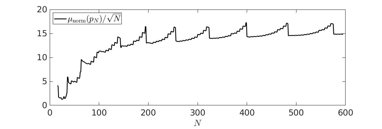
Figure 1. Numerical approximation of $\mu_{\rm norm}(p_{N})/\sqrt{N}$ for $p_{N}$ as in Lemma 1.6 up to degree $595$. The peaks correspond to changes in the value of $M$ as $N$ increases.

Remark 1.7.

Theorem 1.5 shows much more than asked in Problem 1.2 since we get sublinear growth of the condition number. The presence of the (uncomputed) constant $C$ is not an issue since for all but a finite number of values of $N$ we have $C\sqrt{N}\leq N$ and for the first values a simple enumeration of the polynomials with rational coefficients will produce in finite time a polynomial such that $\mu_{\rm norm}(P)\leq N$. Our Theorem 1.5 thus fully answers Problem 1.2 above.

Remark 1.8.

From Lemma 1.1, the condition number of our sequence of polynomials can at most be improved by some constant factor.

1.5. Atomization of the logarithmic potential

Theorem 1.5 will be proved by atomizing the surface measure in $\mathbb{S}^{2}$ and approximating the logarithmic potential of the continuous surface measure by a potential generated by a measure consisting of equal-weighted atoms. This atomization is a well-known technique in non-harmonic Fourier analysis [LyuSod, LyuSeip].

The heuristic argument is that if one places the atoms evenly distributed acording to the surface measure, the discrete potential will mimic the continuous potential which is constant on the sphere and therefore the numerator and the denominator in (7) will both be very similar. Then, the polynomial whose zeros are the inverse stereographic projection of this point set will be well conditioned.

Throughout the paper we denote by $C$ a constant that may be different in each instance that appears. By $f\lesssim g$ we mean that there is a universal constant $C>0$ (i.e. independent of $N$) such that $f\leq Cg$ and we write $f\eqsim g$ if there is a universal constant $C>0$ such that $C^{-1}f\leq g\leq Cf$.

In Section 4 of this paper we describe a construction that satisfies the following result.

Theorem 1.9.

There exists a set $\mathcal{P}_{N}$ of $N$ points in $\mathbb{S}^{2}$ such that if $\operatorname{dist}(p,\mathcal{P}_{N})$ denotes the distance from $p\in\mathbb{S}^{2}$ to $\mathcal{P}_{N}$ and $\kappa=1/2-\log 2.$ Then, for all $p\in\mathbb{S}^{2}$ we have $\sqrt{N}\operatorname{dist}(p,\mathcal{P}_{N})\lesssim 1$ and moreover

(10) $$\sum_{i=1}^{N}\log|p-p_{i}|+\kappa N-\log\left(\sqrt{N}\operatorname{dist}(p,\mathcal{P}_{N})\right)=O(1).$$

Equivalently,

(11) $$\frac{\prod_{i=1}^{N}|p-p_{i}|^{2}}{e^{-2\kappa N}N\operatorname{dist}^{2}(p,\mathcal{P}_{N})}\eqsim 1,\qquad\forall p\in\mathbb{S}^{2},\quad\forall N.$$

Remark 1.10.

In the case that $p=p_{i}$ for some $i\in\{1,\ldots,N\}$, (11) reads

$$\frac{\prod_{j\neq i}^{N}|p_{i}-p_{j}|^{2}}{e^{-2\kappa N}N}\eqsim 1.$$

1.6. Proof of Theorem 1.5

Our main theorem follows immediately from Theorem 1.9 and (7). Indeed, we take the polynomial $P_{N}$ in Theorem 1.9 to be the one whose zeros correspond, under the stereographic projection, to the spherical points $\mathcal{P}_{N}$ in Theorem 1.9 when the points distributed in each parallel of latitude $t$ are rotated to contain the point $(\sqrt{1-t^{2}},0,t)$. As a result, from (7)

$$\mu_{\rm norm}(P_{N})\lesssim\sqrt{N(N+1)}\frac{\sqrt{N}e^{-\kappa N}\left(\int_{\mathbb{S}^{2}}\operatorname{dist}^{2}(p,\mathcal{P}_{N})d\sigma(p)\right)^{1/2}}{\sqrt{N}e^{-\kappa N}}\lesssim\sqrt{N}.$$

2. Organization of the paper

In Section 3 we prove a sharp lower bound for the condition number of any polynomial, Lemma 1.1. In Section 4 we construct the set of points $\mathcal{P}_{N}$ in $\mathbb{S}^{2}$ used in Theorem 1.9 and which give the zeros of the polynomials $P_{N}$ in Theorem 1.5. We study also the separation properties of $\mathcal{P}_{N}.$ In Section 5 we prove some preliminary results comparing the discrete and the continuous potential in a parallel and the potential in three parallels with the potential in a band. Finally we prove Theorem 1.9 at the end of Section 6 as a consequence of the comparison between the discrete potential, the potential in parallels and the continuous potential.

3. Lower bound for the condition number

In this section we prove Lemma 1.1

Proof.

Recall that from (7)

$$\mu_{\rm norm}(P)=\frac{1}{2}\sqrt{N(N+1)}\frac{R}{S},$$

with

$$R=\left(\int_{\mathbb{S}^{2}}\prod_{i=1}^{N}|p-\hat{z}_{i}|\,d\sigma(p)\right)^{1/2},\quad S=\min_{i=1\ldots N}\prod_{j\neq i}|\hat{z}_{i}-\hat{z}_{j}|.$$

Here, $P(z)=\prod_{i=1}^{N}(z-z_{i})$ and $\hat{z}_{i}$ are the associated points in the unit sphere. We bound separately $R$ and $S$. Using Jensen’s inequality we have

$$\log R=\frac{1}{2}\log\int_{\mathbb{S}^{2}}\prod_{i=1}^{N}|p-\hat{z}_{i}|^{2}\,d\sigma(p)\geq\frac{1}{2}\int_{\mathbb{S}^{2}}\log\prod_{i=1}^{N}|p-\hat{z}_{i}|^{2}\,d\sigma(p)=\\ \sum_{i=1}^{N}\int_{\mathbb{S}^{2}}\log|p-\hat{z}_{i}|\,d\sigma(p)=-\kappa N,$$

and hence $R\geq e^{-\kappa N}$. For bounding $S$, note that from (8)

$$-\sum_{\stackrel{{\scriptstyle i,j=1}}{{i\neq j}}}^{N}\log|\hat{z}_{i}-\hat{z}_{j}|\geq\kappa N^{2}-\frac{N}{2}\log N-CN,$$

for some $C>0$. On the other hand,

$$-\sum_{\stackrel{{\scriptstyle i,j=1}}{{i\neq j}}}^{N}\log|\hat{z}_{i}-\hat{z}_{j}|=-\log\left(\prod_{i=1}^{N}\prod_{j\neq i}|\hat{z}_{i}-\hat{z}_{j}|\right)\leq-\log(S^{N})=-N\log S.$$

From

$$-\log(S^{N})\geq\kappa N^{2}-\frac{N}{2}\log N-CN,$$

we get

$$S\lesssim e^{-\kappa N}\sqrt{N},$$

proving $R/S\gtrsim 1/\sqrt{N}.$ The lemma follows. ∎

4. Construction of the point set $\mathcal{P}_{N}$

In this section, we define the set of points $\mathcal{P}_{N}=\{p_{1},\ldots,p_{N}\}\subset\mathbb{S}^{2}$ appearing in Theorem 1.9. The images of these points through the stereographic projection are the zeros of the polynomials in Theorem 1.5. The set $\mathcal{P}_{N}$ will be a union of equidistributed points in symmetric parallels with respect to the $xy$ plane and the construction is similar to the one in [Diamond].

We denote the parallels in $\mathbb{S}^{2}$ by

$$Q_{h}=\{(x,y,z)\in\mathbb{S}^{2}:z=h\},\;\;\;-1\leq h\leq 1.$$

Given $C_{1},C_{2}>0$ and $N\geq 1,$ let $M\geq 1$ and $r_{1},\ldots,r_{M}\in\mathbb{Z}$ be positive integers such that

$$N=2(r_{1}+\ldots+r_{M-1})+r_{M},$$

with

$$C_{1}j\leq r_{j}\leq C_{2}j,$$

for all $1\leq j\leq M.$

Let

$$r_{M+1}=r_{M-1},\ldots,r_{2M-1}=r_{1}.$$

We choose parallel heights $1=H_{0}>H_{1}>\cdots>H_{M-1}>0$ and symmetrically $H_{M+j}=-H_{M-(j+1)}$ for $j=0,\dots,M-1.$ For $1\leq j\leq 2M-1$ we define the bands

$$B_{j}=\{(x,y,z)\in\mathbb{S}^{2}\;\>\;H_{j}\leq z\leq H_{j-1}\},$$

where $B_{1},B_{2M-1}$ are spherical caps. Then $\mathbb{S}^{2}=\bigcup_{j=1}^{2M-1}B_{j}$ and if we define

$$H_{j}=1-\frac{2}{N}\sum_{k=1}^{j}r_{k}\quad 0\leq j\leq 2M-1,$$

we have that

$$\sigma(B_{j})=\frac{H_{j-1}-H_{j}}{2}=\frac{r_{j}}{N},\quad 1\leq j\leq 2M-1.$$

We consider also parallels with heights

$$h_{j}=\frac{H_{j-1}+H_{j}}{2}=H_{j-1}-\frac{r_{j}}{N}=H_{j}+\frac{r_{j}}{N}=1-\frac{2}{N}\sum_{k=1}^{j-1}r_{k}-\frac{r_{j}}{N},$$

for $1\leq j\leq 2M-1,$ and observe that $h_{M}=0$ and $h_{M+j}=-h_{M-j}$ for $j=1,\dots,M-1.$

Observe that for $1\leq j\leq M$

(12) $$1-\frac{C_{2}j^{2}}{N}\leq h_{j}\leq 1-\frac{C_{1}j^{2}}{N},\quad 1-\frac{C_{2}j(j+1)}{N}\leq H_{j}\leq 1-\frac{C_{1}j(j+1)}{N}$$

and

(13) $$-1+\frac{C_{1}j^{2}}{N}\leq h_{2M-j}\leq-1+\frac{C_{2}j^{2}}{N},\quad-1+\frac{C_{1}j(j-1)}{N}\leq H_{2M-j}\leq-1+\frac{C_{2}j(j-1)}{N}.$$

Note that we have

$$C_{1}M^{2}=C_{1}M+2\sum_{j=1}^{M-1}C_{1}j\leq N\leq C_{2}M+2\sum_{j=1}^{M-1}C_{2}j\leq C_{2}M^{2}.$$

We say that a set of points are equidistributed in a parallel if they are, up to homotety, rotation and traslation, a set of roots of unity in the circle defined by the parallel. Given the points $r_{j}$ above we define $\tilde{r}_{1}=\tilde{r}_{2M-1}=0$ and $r_{j}=\tilde{r}_{j}+rem_{j}$ for $2\leq j\leq 2M-2$ where $\tilde{r}_{j}$ is a multiple of $6$ and $0\leq rem_{j}\leq 5.$ Note that in Theorem 1.9 we denote $\tilde{r}_{j}=6s_{j}$. Then to define the set $\mathcal{P}_{N}$

• we take $r_{1}$ points equidistributed in $Q_{h_{1}}$ and similarly $r_{2M-1}=r_{1}$ points equidistributed in $Q_{h_{2M-1}}=Q_{-h_{1}}$.

• For $2\leq j\leq 2M-1$, we take $\frac{4\tilde{r}_{j}}{6}+rem_{j}$ points equidistributed at $Q_{h_{j}},$ $\frac{\tilde{r}_{j-1}+\tilde{r}_{j}}{6}$ points equidistributed in the upper boundary parallel $Q_{H_{j-1}}$ and for $1\leq j\leq 2M-2$ we take $\frac{\tilde{r}_{j}+\tilde{r}_{j+1}}{6}$ points equidistributed in the lower boundary parallel $Q_{H_{j}}.$

Observe that in this way there are $r_{j}$ points of $\mathcal{P}_{N}$ in the band $B_{j}$ for $j=1,\dots,2M-1.$

4.1. Geometric properties of the set $\mathcal{P}_{N}$

From the results in this section it follows that the points in $\mathcal{P}_{N}$ are uniformly separated i.e. for each $p,q\in\mathcal{P}_{N}$ distinct

$$\operatorname{dist}(p,q)\gtrsim 1/\sqrt{N},$$

and they are relatively dense i.e. for all $p\in\mathbb{S}^{2}$ we have that

$$\operatorname{dist}(p,\mathcal{P}_{N})\lesssim 1/\sqrt{N}.$$

Lemma 4.1.

For $h,c\in(-1,1)$ with $|h|\leq|c|$ and $|h-c|\leq 1/4$ we have

$$\operatorname{dist}(Q_{c},Q_{h})\eqsim\frac{|h-c|}{\sqrt{1-h^{2}}}\lesssim\frac{|h-c|}{\sqrt{1-c^{2}}}.$$

Proof.

Note that $\operatorname{dist}(Q_{c},Q_{h})\leq 1$ and we can write also

$$\operatorname{dist}(Q_{c},Q_{h})=2\sin\frac{\varphi}{2},$$

where $\varphi$ is the angular distance from $Q_{c}$ to $Q_{h}$. Moreover,

$$\varphi=2\arcsin\frac{\operatorname{dist}(Q_{c},Q_{h})}{2}\leq 2\arcsin\frac{1}{2}=\frac{\pi}{3}.$$

We first prove the lower bound. Note that for $\varphi\in[0,\pi/3]$

$$\operatorname{dist}(Q_{c},Q_{h})=2\sin\frac{\varphi}{2}\geq\frac{\varphi}{2}\gtrsim|\arcsin(h)-\arcsin(c)|=\frac{|h-c|}{\sqrt{1-\zeta^{2}}}$$

for some $\zeta$ in the interval containing $c$ and $h$. Now, if $c$ and $h$ have both the same sign then $\sqrt{1-\zeta^{2}}\leq\sqrt{1-h^{2}}$ and we are done. Moreover, if $|h|\leq 1/2$ then $|c|\leq 3/4$ and $\sqrt{1-\zeta^{2}}\eqsim 1\eqsim\sqrt{1-h^{2}}$. These are all the cases to cover since $|h-c|\leq 1/4$ excludes other situations. We have proved that $\operatorname{dist}(Q_{c},Q_{h})\gtrsim|h-c|/\sqrt{1-h^{2}}$.

For the upper bound, again using the same argument we can assume that $1/2\leq h\leq c\leq 1$. Then,

$$2\sin\frac{\varphi}{2}\lesssim\sin\varphi=|\sin(\arcsin(h)-\arcsin(c))|=|h\sqrt{1-c^{2}}-c\sqrt{1-h^{2}}|=\\ \frac{c^{2}-h^{2}}{h\sqrt{1-c^{2}}+c\sqrt{1-h^{2}}}\lesssim\frac{c-h}{\sqrt{1-h^{2}}}.$$

∎

Lemma 4.2.

The distance between two points of $\mathcal{P}_{N}$ in the same parallel is or order $1/\sqrt{N}$, i.e.

$$\frac{\sqrt{1-h_{j}^{2}}}{r_{j}}\eqsim\frac{1}{\sqrt{N}},\quad\frac{\sqrt{1-H_{j}^{2}}}{r_{j}}\eqsim\frac{1}{\sqrt{N}}$$

where the first claim is valid for $1\leq j\leq 2M-1$, and the second one is valid for $1\leq j\leq 2M-2.$ In particular, this implies

$$\frac{1-h_{j}^{2}}{1-H_{j}^{2}}\eqsim 1,\quad 1\leq j\leq 2M-2$$

and similarly

$$\frac{1-h_{j}^{2}}{1-H_{j-1}^{2}}\eqsim 1,\quad 2\leq j\leq 2M-1.$$

Proof.

By symmetry we can assume that $j\leq M$. Then, $h_{j}\geq 0$ and hence $\sqrt{1-h_{j}^{2}}\eqsim\sqrt{1-h_{j}}$, which from (12) yields

$$\frac{\sqrt{1-h_{j}^{2}}}{r_{j}}\eqsim\frac{\sqrt{1-h_{j}}}{j}\eqsim\frac{1}{\sqrt{N}}.$$

The inequality for $H_{j}$ is proved in a similar way. ∎

Lemma 4.3.

The distance between consecutive parallels is of order $1/\sqrt{N}$, i.e.

$$\operatorname{dist}(Q_{H_{j-1}},Q_{h_{j}})\eqsim\frac{1}{\sqrt{N}},\quad\operatorname{dist}(Q_{H_{j}},Q_{h_{j}})\eqsim\frac{1}{\sqrt{N}}.$$

Proof.

By symmetry, we can assume that $h_{j}\geq 0$, that implies $|h_{j}|\leq|H_{j-1}|$. From Lemmas 4.1 and 4.2 we have

$$\operatorname{dist}(Q_{H_{j-1}},Q_{h_{j}})\eqsim\frac{r_{j}/N}{\sqrt{1-h_{j}^{2}}}\eqsim\frac{1}{\sqrt{N}}.$$

The other inequality is proved in a similar way. ∎

5. Comparison of discrete potentials, parallels and bands

For $-1\leq h\leq 1$ and $p\in\mathbb{S}^{2}$ we denote

$$f_{p}(h)=\int_{0}^{2\pi}\log|p-\gamma_{h}(\theta)|\,\frac{d\theta}{2\pi},$$

where $\gamma_{h}(\theta)=(\sqrt{1-h^{2}}\cos\theta,\sqrt{1-h^{2}}\sin\theta,h).$ In words, $f_{p}(h)$ is the mean value of $\log|p-q|$ when $q$ lies in the parallel $Q_{h}$. For $-1\leq c,z\leq 1$ we denote

$$R(c,z)=6\sqrt{1-c^{2}}(1-z^{2})+8(1-z^{2})^{3/2}.$$

Lemma 5.1.

Let $\gamma_{h}(\theta)=(\sqrt{1-h^{2}}\cos\theta,\sqrt{1-h^{2}}\sin\theta,h)$, $\theta\in[0,2\pi]$ be a parametrization of $Q_{h}$, and let $p=(a,b,c)\in\mathbb{S}^{2}\setminus Q_{h}$. Then,

$$\left|\frac{d^{3}}{d\theta^{3}}\log|p-\gamma_{h}(\theta)|\right|\leq\frac{\sqrt{1-h^{2}}}{|p-\gamma_{h}(\theta)|}+\frac{R(c,h)}{|p-\gamma_{h}(\theta)|^{3}}.$$

Proof.

We can assume that $p=(\sqrt{1-c^{2}},0,c)$ and denote $\gamma_{h}=\gamma$. Let $F(\theta)=\log|p-\gamma(\theta)|$ and note that, as $\langle\gamma^{\prime}(\theta),\gamma(\theta)\rangle=0$

$$F^{\prime}(\theta)=-\frac{\langle p-\gamma(\theta),\gamma^{\prime}(\theta)\rangle}{|p-\gamma(\theta)|^{2}}=-\frac{\langle p,\gamma^{\prime}(\theta)\rangle}{|p-\gamma(\theta)|^{2}},$$

(14) $$F^{\prime\prime}(\theta)=-\frac{\langle p,\gamma^{\prime\prime}(\theta)\rangle}{|p-\gamma(\theta)|^{2}}-\frac{2\langle p,\gamma^{\prime}(\theta)\rangle^{2}}{|p-\gamma(\theta)|^{4}},$$

and

$$F^{\prime\prime\prime}(\theta)=-\frac{\langle p,\gamma^{\prime\prime\prime}(\theta)\rangle}{|p-\gamma(\theta)|^{2}}-\frac{6\langle p,\gamma^{\prime\prime}(\theta)\rangle\langle p,\gamma^{\prime}(\theta)\rangle}{|p-\gamma(\theta)|^{4}}-\frac{8\langle p,\gamma^{\prime}(\theta)\rangle^{3}}{|p-\gamma(\theta)|^{6}}.$$

Now,

$$|\langle p,\gamma^{\prime}(\theta)\rangle| =|\langle p-\langle p,\gamma(\theta)\rangle\gamma(\theta),\gamma^{\prime}(\theta)\rangle|$$

(15) $$\leq\sqrt{1-\langle p,\gamma(\theta)\rangle^{2}}|\gamma^{\prime}(\theta)|\leq|p-\gamma(\theta)|\sqrt{1-h^{2}},$$

and since $\gamma^{\prime\prime\prime}=-\gamma^{\prime}$ the same bound holds changing $\gamma^{\prime}$ to $\gamma^{\prime\prime\prime}$. Finally, note that

(16) $$|\langle p,\gamma^{\prime\prime}(\theta)\rangle|\leq\sqrt{1-c^{2}}\sqrt{1-h^{2}},$$

and the lemma follows. ∎

Lemma 5.2 (Comparison of the finite sum with the integral along the parallel).

Assume that $\operatorname{dist}(p,Q_{h})\gtrsim\sqrt{1-h^{2}}/A.$ Let $q_{i}\in Q_{h}$ for $i=1,\dots,A$ be points at angular distance $2\pi/A.$ Then

(17) $$\big{|}\sum_{i=1}^{A} \log|p-q_{i}|-Af_{p}(h)\big{|}$$

$$\lesssim\frac{1}{A^{2}}\left(\sqrt{1-h^{2}}\int_{0}^{2\pi}\frac{1}{|p-\gamma_{h}(\theta)|}\,d\theta+R(c,h)\int_{0}^{2\pi}\frac{1}{|p-\gamma_{h}(\theta)|^{3}}\,d\theta\right).$$

Moreover, if $B\supseteq Q_{h}$ is a band of height $\epsilon\lesssim(1-h^{2})/A$ and such that $d(p,B)\gtrsim\frac{\sqrt{1-h^{2}}}{A}$ then

$$\int_{0}^{2\pi}\frac{1}{|p-\gamma_{h}(\theta)|}\,d\theta\eqsim\frac{1}{\sigma(B)}\int_{B}\frac{1}{|p-q|}\,d\sigma(q)$$

and

$$\int_{0}^{2\pi}\frac{1}{|p-\gamma_{h}(\theta)|^{3}}\,d\theta\eqsim\frac{1}{\sigma(B)}\int_{B}\frac{1}{|p-q|^{3}}\,d\sigma(q),$$

where the constants are independent of $h$ and $A.$

Proof.

Without loss of generality, we can assume that $h\geq 0$ and $q_{i}=\gamma_{h}(\theta_{i})$ with $\theta_{i}=(2i-1)\pi/A.$ Define the periodic function $\phi(\theta)=\log|p-\gamma_{h}(\theta)|.$ Since $\phi^{\prime}(\theta)$ is also periodic (17) equals

$$\left|\sum_{i=1}^{A}\right. \left.\phi(\theta_{i})-A\int_{0}^{2\pi}\phi(\theta)\,\frac{d\theta}{2\pi}+\frac{\pi}{12A}\int_{0}^{2\pi}\phi^{\prime\prime}(\theta)\,d\theta\right|$$

$$\leq\sum_{i=1}^{A}\left|\phi(\theta_{i})-\frac{A}{2\pi}\int_{I_{i}}\phi(\theta)\,d\theta+\frac{\pi}{12A}\int_{I_{i}}\phi^{\prime\prime}(\theta)\,d\theta\right|$$

$$\lesssim\frac{1}{A^{3}}\sum_{i=1}^{A}\sup_{\theta\in I_{i}}|\phi^{\prime\prime\prime}(\theta)|\leq\frac{1}{A^{3}}\sum_{i=1}^{A}\sup_{\theta\in I_{i}}\left(\frac{\sqrt{1-h^{2}}}{|p-\gamma_{h}(\theta)|}+\frac{R(c,h)}{|p-\gamma_{h}(\theta)|^{3}}\right)$$

by Lemma A.2 and Lemma 5.1 where $I_{i}=[\theta_{i}-\pi/A,\theta_{i}+\pi/A].$ Let $\theta,\theta^{\prime}\in I_{i}$ be two points were $|p-\gamma_{h}(\cdot)|$ attains respectively its minimum and its maximum value. Then,

$$|p-\gamma_{h}(\theta^{\prime})|\leq |p-\gamma_{h}(\theta)|+|\gamma_{h}(\theta)-\gamma_{h}(\theta^{\prime})|\leq|p-\gamma_{h}(\theta)|+\frac{2\pi\sqrt{1-h^{2}}}{A}$$

$$\lesssim |p-\gamma_{h}(\theta)|+\operatorname{dist}(p,Q_{h})\lesssim|p-\gamma_{h}(\theta)|,$$

and

$$\sup_{\theta\in I_{i}}\left(\frac{\sqrt{1-h^{2}}}{|p-\gamma_{h}(\theta)|}+\frac{R(c,h)}{|p-\gamma_{h}(\theta)|^{3}}\right)\lesssim A\left(\int_{I_{i}}\frac{\sqrt{1-h^{2}}}{|p-\gamma_{h}(\theta)|}d\theta+\int_{I_{i}}\frac{R(c,h)}{|p-\gamma_{h}(\theta)|^{3}}d\theta\right).$$

Now we prove the second part of the lemma. Assume that the band $B$ is the set contained between $Q_{h_{0}}$ and $Q_{h_{0}+2\epsilon}$. For $q\in B$ let $q^{\prime}\in Q_{h}$ be the closest point to $q$ in $Q_{h}$. Then, from Lemma 4.1 we have that $|q-q^{\prime}|\lesssim\epsilon/\sqrt{1-h^{2}}$ and hence

$$|p-q|\leq|p-q^{\prime}|+|q^{\prime}-q|\lesssim|p-q^{\prime}|+\frac{\sqrt{1-h^{2}}}{A}\lesssim|p-q^{\prime}|,$$

and similarly

$$|p-q^{\prime}|\leq|p-q|+|q^{\prime}-q|\lesssim|p-q|+\frac{\sqrt{1-h^{2}}}{A}\lesssim|p-q|.$$

In other words, we have $|p-q|\eqsim|p-q^{\prime}|$ and therefore

$$\int_{B}\frac{1}{|p-q|}d\sigma(q)=\frac{1}{4\pi}\int_{h_{0}}^{h_{0}+2\epsilon}\int_{0}^{2\pi}\frac{1}{|p-\gamma_{t}(\theta)|}d\theta dt\eqsim\epsilon\int_{0}^{2\pi}\frac{1}{|p-\gamma_{h}(\theta)|}d\theta,$$

and we conclude the result after an identical reasoning for the integral of $|p-q|^{-3}$.

∎

Lemma 5.3 (Computation of the integral along one parallel).

Let $p=(a,b,c)\in\mathbb{S}^{2}$. Then,

$$f_{p}(h)=\frac{1}{2}\log(1-hc+|h-c|)=\left\{\begin{array}[]{ll}\frac{1}{2}(\log(1+h)+\log(1-c))&\mbox{if }h\geq c,\\ \\ \frac{1}{2}(\log(1-h)+\log(1+c))&\mbox{if }h<c.\end{array}\right.$$

Proof.

See [LosRusos, 4.224.9]. ∎

Lemma 5.4.

Let $p=(a,b,c)\in\mathbb{S}^{2}$. The following equality holds

$$\int_{0}^{2\pi}\frac{1}{|p-\gamma_{h}(\theta)|^{2}}\,\frac{d\theta}{2\pi}=\frac{1}{2|h-c|}.$$

Proof.

From [LosRusos, 3.661.4] we have

$$\int_{0}^{2\pi}\frac{1}{|p-\gamma_{h}(\theta)|^{2}}\,\frac{d\theta}{2\pi}= \int_{0}^{\pi}\frac{1}{2-2ch-2\sqrt{1-h^{2}}\sqrt{1-c^{2}}\,\cos\theta}\,\frac{d\theta}{\pi}$$

$$= \frac{1}{\sqrt{\left(2-2ch\right)^{2}-\left(2\sqrt{1-h^{2}}\sqrt{1-c^{2}}\right)^{2}}},$$

and the lemma follows after expanding the denominator. ∎

Lemma 5.5 (Comparison of integrals on parallels and bands).

Let $B$ be the band containing $Q_{h}$ given by $B=\{q\in\mathbb{S}^{2}:\langle q,e_{3}\rangle\in[h-\epsilon,h+\epsilon]\}.$ Assume that $h-\epsilon,h+\epsilon\in(-1,1)$ and let $p\in\mathbb{S}^{2}\setminus B$. Then

(18) $$\begin{split}\left|f_{p}(h)-\frac{1}{\epsilon}\int_{B}\log|p-w|\,d\sigma(w)\right|\lesssim\frac{\epsilon^{2}}{(1-\max(|h-\epsilon|,|h+\epsilon|)^{2})^{2}},\end{split}$$

and

(19) $$\begin{split}\left|\frac{f_{p}(h-\epsilon)+4f_{p}(h)+f_{p}(h+\epsilon)}{6}-\frac{1}{\epsilon}\int_{B}\log|p-w|\,d\sigma(w)\right|\lesssim\frac{\epsilon^{4}}{(1-\max(|h-\epsilon|,|h+\epsilon|)^{2})^{4}}.\end{split}$$

Proof.

Using that

$$\frac{1}{\epsilon}\int_{B}\log|p-w|\,d\sigma(w)=\frac{1}{2\epsilon}\int_{h-\epsilon}^{h+\epsilon}f_{p}(t)dt,$$

and Lemma 5.3, the results follows from the error estimation for the midpoint integral rule and for the Simpson rule, see Lemma A.1. Note that we are also using

$$1-\max(|h-\epsilon|,|h+\epsilon|)\eqsim 1-\max(|h-\epsilon|,|h+\epsilon|)^{2}.$$

∎

Lemma 5.6 (Comparison of the integrals on the parallel and the band: the case that the band contains the point $p=(a,b,c)$).

Let $B$ be the band containing $Q_{h}$ given by $B=\{q\in\mathbb{S}^{2}:\langle q,e_{3}\rangle\in[h-\epsilon,h+\epsilon]\}$. Here, we are assuming that $h-\epsilon,h+\epsilon\in(-1,1)$. Then, if $h-\epsilon\leq c\leq h+\epsilon$,

(20) $$\begin{split}\left|f_{p}(h)-\frac{1}{\epsilon}\int_{B}\log|p-w|\,d\sigma(w)\right|\lesssim\frac{\epsilon}{1-c^{2}}.\end{split}$$

and

(21) $$\begin{split}\left|\frac{1}{6}\left(f_{p}(h-\epsilon)+4f_{p}(h)+f_{p}(h+\epsilon)\right)-\frac{1}{\epsilon}\int_{B}\log|p-w|\,d\sigma(w)\right|\lesssim\frac{\epsilon}{1-c^{2}}.\end{split}$$

Proof.

As in the proof of Lemma 5.5, note that

$$\frac{1}{\epsilon}\int_{B}\log|p-w|d\sigma(w)=\frac{1}{2\epsilon}\int_{h-\epsilon}^{h+\epsilon}f_{p}(t)dt=f_{p}(h)+\frac{1}{2\epsilon}\int_{h-\epsilon}^{h+\epsilon}(f_{p}(t)-f_{p}(h))\,dt.$$

Then, the quantity in (20) can be bounded by $2\epsilon$ times the Lipschitz constant $L_{f_{p}}$ of $f_{p}.$ By Lemma 5.3

$$L_{f_{p}}\lesssim\max\left\{\sup_{t\in[h-\epsilon,c]}\frac{1}{1-t},\sup_{t\in[c,h+\epsilon]}\frac{1}{1+t}\right\}\lesssim\frac{1}{1-c}+\frac{1}{1+c}$$

and (20) follows.

In (21) we decompose the Simpson’s rule in the midpoint and the trapezoidal rules. For the midpoint we do as before. For the trapezoidal rule let $\ell(t)$ the line through $(h-\epsilon,f(h-\epsilon))$ and $(h+\epsilon,f(h+\epsilon)).$ To estimate

$$\frac{1}{2\epsilon}\int_{h-\epsilon}^{h+\epsilon}(\ell(t)-f_{p}(t))dt,$$

we use that for $h-\epsilon\leq t\leq h+\epsilon$

$$|\ell(t)-f_{p}(t)|\lesssim(L_{\ell}+L_{f})\epsilon$$

and clearly $L_{\ell}\leq L_{f}.$ ∎

6. The proof of Theorem 1.9

The strategy to prove Theorem 1.9 will follow two steps. First we approximate the potential generated by the surface measure in $\mathbb{S}^{2}$ by a potential generated by a multiple of the length-measure supported in several chosen parallels $Q_{h_{j}}$ and $Q_{H_{j}}.$ Then, we compare the potential in parallels with the discrete potential given by the points in $\mathcal{P}_{N}.$ We follow the notation from Section 4.

6.1. From bands to parallels

We show that, given $p\in\mathbb{S}^{2}$, the mean value of $N\log|p-q|$ for $q\in\mathbb{S}^{2}$ is comparable to the weighted sum of the mean values in different parallels $Q_{h_{j}},Q_{H_{j}}$ where the weights are given by the number of points that we have placed in each parallel.

Proposition 6.1.

Let $p=(a,b,c)\in\mathbb{S}^{2}$ and let $\mathcal{P}_{N}$ be a collection of $N$ points as defined in Section 4. Let

$$S_{N}=r_{1}(f_{p}(h_{1}) +f_{p}(h_{2M-1}))+\sum_{j=2}^{2M-2}\left(\frac{4\tilde{r}_{j}}{6}+rem_{j}\right)f_{p}(h_{j})$$

$$+\sum_{j=1}^{2M-2}\left(\frac{\tilde{r}_{j}+\tilde{r}_{j+1}}{6}\right)f_{p}(H_{j})$$

Then,

$$\left|S_{N}-N\int_{\mathbb{S}^{2}}\log|p-q|\,d\sigma(q)\right|\lesssim 1.$$

Proof.

Assume that $p\in B_{\ell}$ and $\ell\neq 1,2M-1.$ Then we can write the difference above as

(22) $$\sum_{\stackrel{{\scriptstyle j=2}}{{j\neq\ell}}}^{2M-2} \left[\frac{\tilde{r}_{j}}{6}(f_{p}(H_{j-1})+4f_{p}(h_{j})+f_{p}(H_{j}))-\frac{\tilde{r}_{j}}{\sigma(B_{j})}\int_{B_{j}}\log|p-q|d\sigma(q)\right]$$

(23) $$\sum_{\stackrel{{\scriptstyle j=2}}{{j\neq\ell}}}^{2M-2}\left[rem_{j}f_{p}(h_{j})-\frac{rem_{j}}{\sigma(B_{j})}\int_{B_{j}}\log|p-q|d\sigma(q)\right]$$

(24) $$+rem_{\ell}f_{p}(h_{\ell})-\frac{rem_{\ell}}{\sigma(B_{\ell})}\int_{B_{\ell}}\log|p-q|d\sigma(q)$$

(25) $$+\frac{\tilde{r}_{\ell}}{6}(f_{p}(H_{\ell-1})+4f_{p}(h_{\ell})+f_{p}(H_{\ell}))-\frac{\tilde{r}_{\ell}}{\sigma(B_{\ell})}\int_{B_{\ell}}\log|p-q|d\sigma(q)$$

(26) $$+r_{1}(f_{p}(h_{1})+f_{p}(-h_{1}))-\frac{r_{1}}{\sigma(B_{1})}\int_{B_{1}\cup B_{2M-1}}\log|p-q|d\sigma(q).$$

For the first sum (22) we use (19) with $\epsilon=r_{j}/N$ and using from Lemma 4.2 that $j^{2}\eqsim r_{j}^{2}\eqsim N(1-H_{j}^{2})\eqsim N(1-h_{j}^{2})\eqsim N(1-H_{j-1}^{2})$ we get

$$(\ref{x1})\lesssim\sum_{j=2}^{2M-2}\frac{r_{j}^{5}}{N^{4}(1-h_{j}^{2})^{4}}\lesssim\sum_{j=1}^{\infty}\frac{1}{j^{3}}\eqsim 1.$$

For (23) we apply (18) with $\epsilon=r_{j}/N$ and Lemma 4.2 again. Using also that $rem_{j}<6$ and $j^{2}\eqsim r_{j}^{2}\eqsim N(1-h_{j}^{2})$ we get

$$(\ref{x1b})\lesssim\sum_{j=2}^{2M-2}\frac{r_{j}^{2}}{N^{2}(1-h_{j}^{2})^{2}}\lesssim\sum_{j=1}^{\infty}\frac{1}{j^{2}}\eqsim 1.$$

For (24) and (25) we use (20) and (21). This, together with Lemma 4.2 yields

$$(\ref{x2})+(\ref{x3})\lesssim\frac{\tilde{r}_{\ell}}{N(1-c^{2})}+\frac{\tilde{r}_{\ell}^{2}}{N(1-c^{2})}\lesssim\frac{1}{\ell}+1\eqsim 1.$$

Finally, (26)$\eqsim 1$ as follows from Lemma 6.2. ∎

Lemma 6.2.

For any $p\in\mathbb{S}^{2}$ we have

$$\left|f_{p}(h_{1})-\frac{1}{\sigma(B_{1})}\int_{B_{1}}\log|p-q|d\sigma(q)\right|\lesssim 1.$$

Proof.

This follows from a direct computation. If $p\not\in B_{1}$ then the quantity in the lemma is

$$\left|\frac{1}{2}\log(1+h_{1})-\frac{N}{2}\log 2+\frac{N}{2}\log\left(2-\frac{2r_{1}}{N}\right)+\frac{1}{2}\log\left(2-\frac{2r_{1}}{N}\right)\right|\lesssim 1,$$

since $\log\left(2-\frac{2r_{1}}{N}\right)-\log 2=\log\left(1-\frac{2r_{1}}{N}\right)\eqsim 1/N$. If $p\in B_{1}$ it is a little longer computation. One must write

$$\int_{B_{1}}\log|p-q|d\sigma(q)=\int_{1-2r_{1}/N}^{1}f_{p}(t)\,dt,$$

and consider two subintervals depending on $t<\langle p,e_{3}\rangle$ or $t>\langle p,e_{3}\rangle$. Then, from Lemma 5.3 this quantity can be computed exactly and the lemma follows after some elementary manipulations. ∎

6.2. From points to parallels

In this section we prove Theorem 1.9. Recall that the sum for all parallels $S_{N}$ defined in Proposition 6.1. Then,

$$\sum_{p_{i}\in\mathcal{P}_{N}} \log|p-p_{i}|-S_{N}$$

$$=\sum_{p_{i}\in Q_{h_{1}}\cup Q_{h_{2M-1}}}\log|p-p_{i}|-r_{1}(f_{p}(h_{1})+f_{p}(h_{2M-1}))$$

$$+\sum_{j=2}^{2M-2}\left[\sum_{p_{i}\in Q_{h_{j}}}\log|p-p_{i}|-\left(\frac{4\tilde{r}_{j}}{6}+rem_{j}\right)f_{p}(h_{j})\right]$$

$$+\sum_{j=1}^{2M-2}\left[\sum_{p_{i}\in Q_{H_{j}}}\log|p-p_{i}|-\left(\frac{\tilde{r}_{j}+\tilde{r}_{j+1}}{6}\right)f_{p}(H_{j})\right].$$

We will bound in a different way the terms corresponding to three situations: that the parallel ($Q_{h_{j}}$ or $Q_{H_{j}}$) is very close to $p$, moderately close to $p$ and far away from $p$.

6.2.1. The closest parallel

We will bound the term corresponding to the parallel containing the closest point to $p$ using the following lemma. If there is more than one parallel with this property, we can apply the lemma to any of them.

Lemma 6.3.

Let $p\in\mathbb{S}^{2}$ and let $p_{i_{0}}\in\mathcal{P}_{N}$ be the closest point to $p$. Assume that $p_{i_{0}}\in Q_{h_{\ell}}$. Then

$$\left|\sum_{\stackrel{{\scriptstyle p_{i}\in Q_{h_{\ell}}}}{{i\neq i_{0}}}}\log|p-p_{i}|-\left(\frac{4\tilde{r}_{\ell}}{6}+rem_{\ell}\right)f_{p}(h_{\ell})-\log\sqrt{N}\right|\lesssim 1.$$

Similarly, if $p_{i_{0}}\in Q_{H_{\ell}}$, then

$$\left|\sum_{\stackrel{{\scriptstyle p_{i}\in Q_{H_{\ell}}}}{{i\neq i_{0}}}}\log|p-p_{i}|-\left(\frac{\tilde{r}_{\ell}+\tilde{r}_{\ell+1}}{6}\right)f_{p}(H_{\ell})-\log\sqrt{N}\right|\lesssim 1.$$

Proof.

Since the proof of both inequalities is equal, we just prove the first one and we use the notation $Q_{\ell}=Q_{h_{\ell}}$, $\gamma_{\ell}=\gamma_{h_{\ell}}$ and $c_{\ell}=4\tilde{r}_{\ell}/6+rem_{\ell}\eqsim\ell.$ We rename $\mathcal{P}_{N}\cap Q_{\ell}=\{q_{1},\dots,q_{c_{\ell}}\}$ and we call $q_{1}$ the closest point to $p,$ with the former notation, $p_{i_{0}}=q_{1}.$ We split the parallel $Q_{\ell}$ in arcs $\gamma_{\ell}(I_{j})$ centered on each $q_{j}$ with angle $\frac{2\pi}{c_{\ell}}$. With this notation, the sum in the lemma –without the $\log\sqrt{N}$ term– is

$$\sum_{\stackrel{{\scriptstyle p_{i}\in Q_{\ell}}}{{i\neq i_{0}}}}\log|p-p_{i}|-c_{\ell}f_{p}(h_{\ell})= \sum_{j=2}^{c_{\ell}}\log|p-q_{j}|-\frac{c_{\ell}}{2\pi}\sum_{j=2}^{c_{\ell}}\int_{I_{j}}\log|p-\gamma_{\ell}(\theta)|d\theta$$

$$-\frac{c_{\ell}}{2\pi}\int_{I_{1}}\log|p-\gamma_{\ell}(\theta)|d\theta.$$

First we estimate this last integral. By a rotation we assume that $\gamma_{\ell}(I_{1})$ is centered at the point $\tilde{q}_{1}=(\sqrt{1-h_{\ell}^{2}},0,h_{\ell})$ and we denote the rotated arc by $I.$ By this rotation the point $p$ goes to some other point $\tilde{p}.$ Observe that to estimate the integral

$$-\frac{c_{\ell}}{2\pi}\int_{I}\log|\tilde{p}-\gamma_{\ell}(\theta)|d\theta,$$

from above, we can replace $\tilde{p}$ by the point $\tilde{q}_{1}.$ Indeed,

$$\Delta_{u}(\log|u-q|)=2\pi\delta_{q}-2\pi d\sigma,$$

where $\Delta_{u}$ is the Laplace-Beltrami operator with respect to the variable $u$ and $\delta_{u}$ is Dirac’s delta. Therefore, out of $q\in\gamma_{\ell}(I),$ the function $-\log|r-q|$ is subharmonic and satisfies the maximum principle

$$\sup_{u\in\mathbb{S}^{2}\setminus I}\int_{I}\log\frac{1}{|u-\gamma_{\ell}(\theta)|}d\theta\leq\sup_{u\in I}\int_{I}\log\frac{1}{|u-\gamma_{\ell}(\theta)|}d\theta.$$

Clearly, this last integral is smaller that

$$\int_{I}\log\frac{1}{|\tilde{q}_{1}-\gamma_{\ell}(\theta)|}d\theta.$$

Using this observation we get for some constant $C>0$ (whose value may vary en each appearance):

$$-\frac{c_{\ell}}{2\pi}\int_{I}\log|\tilde{p}-\gamma_{\ell}(\theta)|d\theta \leq-\frac{c_{\ell}}{2\pi}\int_{I}\log|\tilde{q}_{1}-\gamma_{\ell}(\theta)|d\theta=-\frac{c_{\ell}}{4\pi}\int_{-\frac{\pi}{c_{\ell}}}^{\frac{\pi}{c_{\ell}}}\log(1-\cos\theta)d\theta$$

$$-\frac{1}{2}\log(1-h_{\ell}^{2})+C\leq-\frac{c_{\ell}}{\pi}\int_{0}^{\frac{\pi}{c_{\ell}}}\log\theta d\theta-\frac{1}{2}\log(1-h_{\ell}^{2})+C$$

$$\leq\log\frac{c_{\ell}}{\sqrt{1-h_{\ell}^{2}}}+C\leq\log\sqrt{N}+C,$$

where we use that $-\log(1-\cos\theta)\leq\log(4/\theta^{2})$ in the range $\theta\in[-\pi/2,\pi/2]$ and Lemma 4.2. We also have a similar lower bound coming from the fact that $|p-\gamma_{\ell}(\theta)|\lesssim 1/\sqrt{N}$ for $\theta\in I_{1}$:

$$-\frac{c_{\ell}}{2\pi}\int_{I}\log|\tilde{p}-\gamma_{\ell}(\theta)|d\theta\geq\frac{c_{\ell}}{2\pi}\int_{I}\log\sqrt{N}d\theta-C=\log\sqrt{N}-C.$$

In other words, we have proved that

$$\left|-\frac{c_{\ell}}{2\pi}\int_{I}\log|\tilde{p}-\gamma_{\ell}(\theta)|d\theta-\log\sqrt{N}\right|\lesssim 1.$$

A similar argument shows that

$$\left|-\frac{c_{\ell}}{2\pi}\int_{I_{j}}\log|\tilde{p}-\gamma_{\ell}(\theta)|d\theta-\log|p-q_{j}|\right|\lesssim 1$$

for any $j\neq 1$. This allows us to remove any constant number of terms of the sum in the lemma for proving the bound. We thus have to bound

(27) $$\left|\sum_{j\in J}\log|p-q_{j}|-\frac{c_{\ell}}{2\pi}\sum_{j\in J}\int_{I_{j}}\log|p-\gamma_{\ell}(\theta)|d\theta\right|,$$

where $J$ is the set of indices $j\in\{1,\ldots,c_{\ell}\}$ such that $\operatorname{dist}(p,\gamma_{\ell}(I_{j}))\geq 1/\sqrt{N}$. Now, for such $j$ we can apply the classical estimate for the midpoint rule in Lemma A.1 getting

$$\left|\log|p-q_{j}|-\frac{c_{\ell}}{2\pi}\int_{I_{j}}\log|p-\gamma_{\ell}(\theta)|d\theta\right|\lesssim\frac{1}{c_{\ell}^{2}}\sup_{\theta\in I_{j}}\left|\frac{d^{2}}{d\theta^{2}}(\log|p-\gamma_{\ell}(\theta)|)\right|.$$

This second derivative has been computed in (14) and can be bounded using (16) and (5) thus proving that

$$\left|\log|p-q_{j}|-\frac{c_{\ell}}{2\pi}\int_{I_{j}}\log|p-\gamma_{\ell}(\theta)|d\theta\right|\lesssim\frac{1}{c_{\ell}^{2}}\sup_{\theta\in I_{j}}\frac{1-h_{\ell}^{2}+\sqrt{1-h_{\ell}^{2}}\sqrt{1-c^{2}}}{|p-\gamma_{\ell}(\theta)|^{2}}.$$

But $\sqrt{1-c^{2}}\lesssim\sqrt{1-h_{\ell}^{2}}$ and since $j\in J$ we have $|p-\gamma_{\ell}(\theta)|\eqsim|p-q_{j}|$ for all $\theta\in I_{j}$, which yields

$$\left|\log|p-q_{j}|-\frac{c_{\ell}}{2\pi}\int_{I_{j}}\log|p-\gamma_{\ell}(\theta)|d\theta\right|\lesssim\frac{1}{c_{\ell}^{2}}\frac{1-h_{\ell}^{2}}{|p-q_{j}|^{2}}.$$

Recall that $\operatorname{dist}(p,\mathcal{P}_{N})=|p-p_{1}|$ and the points $p_{j}$ in the parallel $Q_{\ell}$ are separated by a constant times $N^{-1/2}$ and hence

$$|\tilde{p}-\tilde{q}_{j}|=|p-q_{j}|\gtrsim\frac{j}{\sqrt{N}},\quad 1\leq j\leq\frac{c_{\ell}}{2},$$

with a similar inequality for $c_{\ell}/2\leq j\leq c_{\ell}$. We thus conclude that

$$\left|\log|p-q_{j}|-\frac{c_{\ell}}{2\pi}\int_{I_{j}}\log|p-\gamma_{\ell}(\theta)|d\theta\right|\lesssim\frac{1}{c_{\ell}^{2}}\frac{N(1-h_{\ell}^{2})}{j^{2}}\eqsim\frac{1}{j^{2}},$$

the last from Lemma 4.2. We conclude that

$$\eqref{eq:ultima}\lesssim\sum_{j\in J}\frac{1}{j^{2}}\lesssim 1,$$

and thus the result. ∎

6.2.2. Parallels that are moderately close to $p$

If $p\in B_{\ell}$, we will bound the terms corresponding to the parallels in $B_{\ell-1},B_{\ell}$ and $B_{\ell+1}$ (with the exception of the closest parallel to $p$, that we have already dealt with) using the following lemma.

Lemma 6.4.

Let $p\in\mathbb{S}^{2}$. Then, for any $j=1,\ldots,2M-1$ such that $\operatorname{dist}(p,Q_{h_{j}})\gtrsim 1/\sqrt{N}$ then

$$\left|\sum_{p_{i}\in Q_{h_{j}}}\log|p-p_{i}|-\left(\frac{4\tilde{r}_{j}}{6}+rem_{j}\right)f_{p}(h_{j})\right|\lesssim 1.$$

Similarly, for any $j=1,\ldots,2M-2$ such that $\operatorname{dist}(p,Q_{H_{j}})\gtrsim 1/\sqrt{N}$ we have

$$\left|\sum_{p_{i}\in Q_{H_{j}}}\log|p-p_{i}|-\left(\frac{\tilde{r}_{j}+\tilde{r}_{j+1}}{6}\right)f_{p}(H_{j})\right|\lesssim 1.$$

Proof.

We prove the first inequality since both follow from the same argument. From Lemma 5.2 and denoting $p=(a,b,c)$ we just need to show that $I_{1}+I_{2}+I_{3}\lesssim 1$ where

$$I_{1}= \frac{\sqrt{1-h_{j}^{2}}}{j^{2}}\int_{0}^{2\pi}\frac{1}{|p-\gamma_{h_{j}}(\theta)|}\,d\theta,$$

$$I_{2}= \frac{\sqrt{1-c^{2}}(1-h_{j}^{2})}{j^{2}}\int_{0}^{2\pi}\frac{1}{|p-\gamma_{h_{j}}(\theta)|^{3}}\,d\theta,$$

$$I_{3}= \frac{(1-h_{j}^{2})^{3/2}}{j^{2}}\int_{0}^{2\pi}\frac{1}{|p-\gamma_{h_{j}}(\theta)|^{3}}\,d\theta.$$

Now, from Lemmas 4.2, 5.4 and 4.1 and the hypotheses of the lemma we have

$$I_{1}\lesssim \frac{1}{j\sqrt{N}}\int_{0}^{2\pi}\frac{1}{|p-\gamma_{h_{j}}(\theta)|}\,d\theta\lesssim\frac{1}{j}\lesssim 1,$$

$$I_{2}\lesssim \frac{\sqrt{1-c^{2}}}{\sqrt{N}}\int_{0}^{2\pi}\frac{1}{|p-\gamma_{h_{j}}(\theta)|^{2}}\,d\theta\lesssim\frac{\sqrt{1-c^{2}}}{\sqrt{N}|h_{j}-c|}\lesssim 1,$$

$$I_{3}\lesssim \frac{\sqrt{1-h_{j}^{2}}}{\sqrt{N}}\int_{0}^{2\pi}\frac{1}{|p-\gamma_{h_{j}}(\theta)|^{2}}\,d\theta\lesssim\frac{\sqrt{1-h_{j}^{2}}}{\sqrt{N}|h_{j}-c|}\lesssim 1.$$

∎

6.2.3. Parallels that are far from $p$

Finally, assuming that $p\in B_{\ell}$, we bound the terms corresponding to the parallels $Q_{h_{j}}$ and $Q_{H_{j}}$ that do not touch $B_{\ell-1},B_{\ell}$ or $B_{\ell+1}$. We can therefore assume that we are under the hypotheses of Lemma 5.2, that is, that for some constant $C>0$ we have

$$\operatorname{dist}(p,B_{j})\geq\frac{C}{\sqrt{N}}\geq\frac{C\sqrt{1-h_{j}^{2}}}{r_{j}}.$$

We now prove the following result.

Lemma 6.5.

If $p\in B_{\ell}$ then

$$\sum_{\stackrel{{\scriptstyle j=2}}{{j\neq\ell-1,\ell,\ell+1}}}^{2M-2}\left[\sum_{p_{i}\in Q_{h_{j}}}\log|p-p_{i}|-\left(\frac{4\tilde{r}_{j}}{6}+rem_{j}\right)f_{p}(h_{j})\right]\lesssim 1.$$

Similarly,

$$\sum_{\stackrel{{\scriptstyle j=2}}{{j\neq\ell-1,\ell,\ell+1}}}^{2M-2}\left[\sum_{p_{i}\in Q_{H_{j}}}\log|p-p_{i}|-\left(\frac{\tilde{r}_{j}+\tilde{r}_{j+1}}{6}\right)f_{p}(H_{j})\right]\lesssim 1.$$

Proof.

We just prove the first assertion, since the second one is proved the same way. Lemma 5.2 yields

$$\sum_{\stackrel{{\scriptstyle j=2}}{{j\neq\ell-1,\ell,\ell+1}}}^{2M-2}\left[\sum_{p_{i}\in Q_{h_{j}}}\log|p-p_{i}|-\left(\frac{4\tilde{r}_{j}}{6}+rem_{j}\right)f_{p}(h_{j})\right]\lesssim\\ \sum_{\stackrel{{\scriptstyle j=2}}{{j\neq\ell-1,\ell,\ell+1}}}^{2M-1}\frac{1}{j}\left(\frac{1}{\sqrt{1-h_{j}^{2}}}\int_{B_{j}}\frac{1}{|p-q|}d\sigma(q)+\frac{R(c,h_{j})}{1-h_{j}^{2}}\int_{B_{j}}\frac{1}{|p-q|^{3}}d\sigma(q)\right).$$

We split this last sum in three parts

$$T_{1}= \sum_{j\neq\ell-1,\ell,\ell+1}\frac{1}{j\sqrt{1-h_{j}^{2}}}\int_{B_{j}}\frac{1}{|p-q|}\,d\sigma(q),$$

$$T_{2}= \sum_{j\neq\ell-1,\ell,\ell+1}\frac{\sqrt{1-c^{2}}}{j}\int_{B_{j}}\frac{1}{|p-q|^{3}}\,d\sigma(q),$$

$$T_{3}= \sum_{j\neq\ell-1,\ell,\ell+1}\frac{\sqrt{1-h_{j}^{2}}}{j}\int_{B_{j}}\frac{1}{|p-q|^{3}}\,d\sigma(q).$$

The easiest one is $T_{3}$, since from Lemma 4.2 we have:

(28) $$T_{3}\lesssim\frac{1}{\sqrt{N}}\sum_{j\neq\ell-1,\ell,\ell+1}\int_{B_{j}}\frac{1}{|p-q|^{3}}d\sigma(q)\lesssim\frac{1}{\sqrt{N}}\int_{\mathbb{S}^{2}\setminus B(p,C/\sqrt{N})}\frac{1}{|p-q|^{3}}d\sigma(q)=\\ \frac{1}{\sqrt{N}}\int_{-1}^{1-C^{2}/(2N)}\frac{1}{(1-t)^{3/2}}\,dt\lesssim 1,$$

where, recall, $B(p,C/\sqrt{N})$ is a spherical cap around $p$ of radius $C/\sqrt{N}$.

Now, for $T_{2}$, for those $j$ such that $\sqrt{1-c^{2}}\leq\sqrt{1-h_{j}^{2}}$ we apply the previous argument. In other case, again from Lemma 4.2, we have

$$T_{2} \lesssim\frac{1}{\sqrt{N}}\sum_{j\neq\ell-1,\ell,\ell+1}\frac{\sqrt{1-c^{2}}}{\sqrt{1-h_{j}^{2}}}\int_{B_{j}}\frac{1}{|p-q|^{3}}\,d\sigma(q)$$

$$=\frac{1}{\sqrt{N}}\sum_{j\neq\ell-1,\ell,\ell+1}\frac{|p-e_{3}||p+e_{3}|}{|q_{h_{j}}-e_{3}||q_{h_{j}}+e_{3}|}\int_{B_{j}}\frac{1}{|p-q|^{3}}\,d\sigma(q)$$

where we are using that for any point $q_{h}\in Q_{h}$ we have

$$\sqrt{1-h^{2}}=|q_{h}-e_{3}||q_{h}+e_{3}|/2.$$

For any $q\in B_{j}$ we have that

$$|q_{h_{j}}\pm e_{3}|\gtrsim|q\pm e_{3}|.$$

And we thus conclude that

$$T_{2}\lesssim\frac{1}{\sqrt{N}}\sum_{j\neq\ell-1,\ell,\ell+1}\int_{B_{j}}\frac{|p-e_{3}||p+e_{3}|}{|p-q|^{3}|q-e_{3}||q+e_{3}|}\,d\sigma(q).$$

By a symmetry argument and using $|p-e_{3}|\leq|p-q|+|q-e_{3}|$ it suffices to bound

$$\frac{1}{\sqrt{N}}\int_{\{q\in\mathbb{S}^{2}:|p-q|\geq C/\sqrt{N}\}}\left(\frac{1}{|p-q|^{2}|q-e_{3}|}+\frac{1}{|p-q|^{3}}\right)\,d\sigma(q),$$

for a certain constant $C>0.$ Following the same argument as the one used for $T_{3}$ it is enough to consider

$$\frac{1}{\sqrt{N}}\int_{\{q\in\mathbb{S}^{2}:|p-q|\geq C/\sqrt{N}\}}\frac{1}{|p-q|^{2}|q-e_{3}|}d\sigma(q)\leq\\ \frac{1}{\sqrt{N}}\int_{\{q\in\mathbb{S}^{2}:|p-q|\geq C/\sqrt{N},|q-e_{3}|\geq 1/\sqrt{N}\}}\frac{1}{|p-q|^{2}|q-e_{3}|}d\sigma(q)\\ +\frac{1}{\sqrt{N}}\int_{\{q\in\mathbb{S}^{2}:|p-q|\geq C/\sqrt{N},|q-e_{3}|\leq 1/\sqrt{N}\}}\frac{1}{|p-q|^{2}|q-e_{3}|}d\sigma(q).$$

The first of these two integrals is from Hölder’s inequality at most

$$\left(\int_{\{q\in\mathbb{S}^{2}:|p-q|\geq C/\sqrt{N}\}}\frac{1}{|p-q|^{3}}\,d\sigma(q)\right)^{2/3}\left(\int_{\{q\in\mathbb{S}^{2}:|q-e_{3}|\geq 1/\sqrt{N}\}}\frac{1}{|q-e_{3}|^{3}}\,d\sigma(q)\right)^{1/3},$$

which is bounded above again by a constant times $\sqrt{N}$ as already seen in 28. We bound the second integral as

$$N\int_{\{q\in\mathbb{S}^{2}:|q-e_{3}|\leq 1/{\sqrt{N}}\}}\frac{1}{|q-e_{3}|}\,d\sigma(q)\lesssim N\int_{1-\frac{2}{N}}^{1}\frac{1}{\sqrt{1-t}}\,dt\lesssim\sqrt{N}.$$

It remains to bound $T_{1}$. Again from Lemma 4.2 we have

$$T_{1}\lesssim\frac{1}{\sqrt{N}}\sum_{j\neq\ell-1,\ell,\ell+1}\frac{1}{1-h_{j}^{2}} \int_{B_{j}}\frac{1}{|p-q|}\,d\sigma(q)\lesssim\sqrt{N}\int_{B_{1}\cup B_{2M-1}}\frac{1}{|p-q|}\,d\sigma(q)$$

$$+ \frac{1}{\sqrt{N}}\left[\sum_{j=2}^{\ell-2}+\sum_{j=\ell+2}^{2M-2}\right]\frac{1}{1-h_{j}^{2}}\int_{B_{j}}\frac{1}{|p-q|}\,d\sigma(q),$$

where we have used that $1-h_{j}^{2}\gtrsim 1/N$. The first integral is easily bounded by

$$\int_{q\in B_{1}\cup B_{2M-1}}\frac{1}{|p-q|}\,d\sigma(q)\leq\int_{B_{1}}\frac{1}{|e_{3}-q|}\,d\sigma(q)+\int_{B_{2M-1}}\frac{1}{|e_{3}+q|}\,d\sigma(q)\lesssim\frac{1}{\sqrt{N}}.$$

Finally, from the same arguments as above we have to bound

$$\frac{1}{\sqrt{N}}\int_{\{q\in\mathbb{S}^{2}:|p-q|\geq C/\sqrt{N},|q\pm e_{3}|\geq C^{\prime}/\sqrt{N}\}}\frac{1}{|p-q||q-e_{3}|^{2}|q+e_{3}|^{2}}\,d\sigma(q),$$

where $C,C^{\prime}$ are positive constants and it is enough to check that

$$\int_{\{q\in\mathbb{S}^{2}:|p-q|\geq C/\sqrt{N},|q-e_{3}|\geq C^{\prime}/\sqrt{N}\}}\frac{1}{|p-q||q-e_{3}|^{2}}\,d\sigma(q),$$

$$\int_{\{q\in\mathbb{S}^{2}:|p-q|\geq C/\sqrt{N},|q+e_{3}|\geq C^{\prime}/\sqrt{N}\}}\frac{1}{|p-q||q+e_{3}|^{2}}\,d\sigma(q),$$

are $O(\sqrt{N}).$ This again follows from Hölder’s inequality. ∎

6.3. Proof of Theorem 1.9

We are now ready to finish the proof. By Proposition 6.1

$$\sum_{i=1}^{N} \log|p-p_{i}|=\sum_{\stackrel{{\scriptstyle i=1}}{{i\neq i_{0}}}}^{N}\log|p-p_{i}|+\log\operatorname{dist}(p,\mathcal{P}_{N})=-\kappa N+\log\left(\sqrt{N}\operatorname{dist}(p,\mathcal{P}_{N})\right)$$

$$+\sum_{p_{i}\not\in Q_{\ell}}\log|p-p_{i}|-S_{N}(\ell)+\sum_{\stackrel{{\scriptstyle p_{i}\in Q_{\ell}}}{{i\neq i_{0}}}}\log|p-p_{i}|-c_{\ell}f_{p}(h_{\ell})-\frac{1}{2}\log N+O(1),$$

where $S_{N}(\ell)$ is the sum $S_{N}$ without the part corresponding to the parallel $Q_{\ell}$ and $c_{\ell}\eqsim\ell$ is the number of points in parallel $Q_{\ell}$. From Lemmas 6.3, 6.4 and 6.5 we conclude that

$$\left|\sum_{i=1}^{N}\log|p-p_{i}|+\kappa N-\log\left(\sqrt{N}\operatorname{dist}(p,\mathcal{P}_{N})\right)\right|\lesssim 1,$$

as wanted.

Appendix A The error of the mid-point rule for numerical integration

Recall the following classical estimates for the midpoint and Simpson integration rules.

Lemma A.1.

Let $f:[a,b]\to\mathbb{R}$ be a $C^{2}$ function. Then,

$$\left|\int_{a}^{b}f(x)\,dx-(b-a)f\left(\frac{a+b}{2}\right)\right|\leq\frac{(b-a)^{3}\|f^{(2)}\|_{\infty}}{24}.$$

Moreover, if $f$ is $C^{4}$ then,

$$\left|\int_{a}^{b}f(x)\,dx-\frac{b-a}{6}\left(f(a)+4f\left(\frac{a+b}{2}\right)+f(b)\right)\right|\leq\frac{(b-a)^{5}\|f^{(4)}\|_{\infty}}{2880}.$$

We also need the following more sophisticated version of the midpoint rule.

Lemma A.2.

Let $f:[a,b]\to\mathbb{R}$ be a $C^{3}$ function. Then,

$$\left|\int_{a}^{b}f(x)\,dx-(b-a)f\left(\frac{a+b}{2}\right)-\frac{(b-a)^{2}}{24}\int_{a}^{b}f^{\prime\prime}(x)\,dx\right|\leq\frac{(b-a)^{4}\|f^{(3)}\|_{\infty}}{64}.$$

Proof.

We first assume that $[a,b]=[-1,1]$. Let $S$ be the quantity to be estimated in this lemma. Expanding with Taylor series

$$f(x)=f(0)+f^{\prime}(0)x+\frac{1}{2}f^{\prime\prime}(0)x^{2}+\frac{1}{6}f^{(3)}(\zeta_{x})x^{3}.$$

$$f^{\prime\prime}(x)=f^{\prime\prime}(0)+f^{(3)}(\eta_{x})x,$$

then the quantity to be estimated is

$$\left|\int_{-1}^{1}\frac{1}{2}f^{\prime\prime}(0)x^{2}+\frac{1}{6}f^{(3)}(\zeta_{x})x^{3}\,dx-\frac{2f^{\prime\prime}(0)}{6}-\frac{1}{6}\int_{-1}^{1}f^{(3)}(\eta_{x})x\,dx\right|\leq\frac{\|f^{(3)}\|_{\infty}}{4}.$$

For general $[a,b]$ one can apply the previous result to $g:[-1,1]\to\mathbb{R}$ given by $g(t)=f((a+b)/2+t(b-a)/2)$. ∎