Asymptotics of MAP Inference in Deep Networks

Abstract

Deep generative priors are a powerful tool for reconstruction problems with complex data such as images and text. Inverse problems using such models require solving an inference problem of estimating the input and hidden units of the multi-layer network from its output. Maximum a priori (MAP) estimation is a widely-used inference method as it is straightforward to implement, and has been successful in practice. However, rigorous analysis of MAP inference in multi-layer networks is difficult. This work considers a recently-developed method, multi-layer vector approximate message passing (ML-VAMP), to study MAP inference in deep networks. It is shown that the mean squared error of the ML-VAMP estimate can be exactly and rigorously characterized in a certain high-dimensional random limit. The proposed method thus provides a tractable method for MAP inference with exact performance guarantees.

I Introduction

We consider inference in an $L$ layer stochastic neural network of the form,

$$\mathbf{z}^{0}_{\ell} =\mathbf{W}_{\ell}\mathbf{z}^{0}_{\ell\!-\!1}+\mathbf{b}_{\ell}+{\bm{\xi}}_{\ell},\quad\ell=1,3,\ldots,L\!-\!1$$ (1a)

$$\mathbf{z}^{0}_{\ell} ={\bm{\phi}}_{\ell}(\mathbf{z}^{0}_{\ell\!-\!1},{\bm{\xi}}_{\ell}),\quad\ell=2,4,\ldots,L.$$ (1b)

where $\mathbf{z}^{0}_{0}$ is the initial input, $\mathbf{z}^{0}_{\ell}$, $\ell=1,\ldots,L-1$ are the intermediate hidden unit outputs and $\mathbf{y}=\mathbf{z}^{0}_{L}$ is the output. The number of layers $L$ is even. The equations (1a) correspond to linear (fully-connected) layers with weights and biases $\mathbf{W}_{\ell}$ and $\mathbf{b}_{\ell}$, while (1b) correspond to elementwise activation functions such as sigmoid or ReLU. The signals ${\bm{\xi}}_{\ell}$ represent noise terms. A block diagram for the network is shown in the top panel of Fig. 1. The inference problem is to estimate the initial and hidden states $\mathbf{z}^{0}_{\ell}$, $\ell=0,\ldots,L\!-\!1$ from the final output $\mathbf{y}$. We assume that network parameters (the weights, biases and activation functions) are all known (i.e. already trained). Hence, this is not the learning problem. The superscript 0 in $\mathbf{z}^{0}_{\ell}$ indicates that these are the “true" values, to be distinguished from estimates that we will discuss later.

This inference problem arises commonly when deep networks are used as generative priors. Deep neural networks have been extremely successful in providing probabilistic generative models of complex data such as images, audio and text. The models can be trained either via variational autoencoders [1, 2] or generative adversarial networks [3, 4]. In inverse problems, a deep network is used as a generative prior for the data (such as an image) and additional layers are added to model the measurements (such as blurring, occlusion or noise) [5, 6]. Inference can then be used to reconstruct the original image from the measurements.

Figure 1: Top panel: Feedfoward neural network mapping an input $\mathbf{z}_{0}$ to output $\mathbf{y}$ in the case of $L=4$ layers. Bottom panel: ML-VAMP inference algorithm for recovering estimates for the input and hidden states from the output $\mathbf{y}$.

Many deep network-based reconstruction methods perform maximum a priori (MAP) estimation via minimization of the negative log likelihood [5, 6] or an equivalent regularized least-squares objective [7]. MAP minimization is readily implementable and has worked successfully in practice in problems such as inpainting and compressed sensing. MAP estimation also provides an alternative to a separately learned reconstruction network such as [8, 9, 10]. However, due to the non-convex nature of the objective function, MAP estimation has been difficult to analyze rigorously. For example, results such as [11] provide only general scaling laws while the guarantees in [12] require that a non-convex projection operation can be performed exactly.

To better understand MAP-based reconstruction, this work considers inference in deep networks via approximate message passing (AMP). AMP [13] and its variants refer to a powerful class of techniques for inverse problems that are both computationally efficient and admit provable guarantees in certain high-dimensional limits. Recent works [14, 15, 16, 17] have developed and analyzed variants of AMP for inference in multi-layer networks such as (1). The methods generally consider minimum mean squared error (MMSE) inference and estimation of the posterior density of the hidden units $\mathbf{z}_{\ell}$ from $\mathbf{y}$. Similar to other AMP methods, such MMSE-based multi-layer versions of AMP can be rigorously analyzed in cases with with large random transforms. This work specifically considers an extension of the multi-layer vector AMP (ML-VAMP) method proposed in [15]. ML-VAMP is derived from the recently-developed VAMP method of [18, 19, 20] which is itself based on expectation propagation [21] and expectation consistent approximate inference [22, 23]. Importantly, in the case of large random transforms, it is shown in [15] that the reconstruction error of ML-VAMP with MMSE estimation can be exactly predicted, enabling much sharper results than other analysis techniques. Moreover, under certain testable conditions ML-VAMP can provably asymptotically achieve the Bayes optimal estimate, even for non-convex problems.

However, MAP estimation is often preferable to MMSE inference since MAP can be formulated as an unconstrained optimization and implemented easily via standard deep learning optimizers [5, 6, 7]. This work thus considers a MAP version of ML-VAMP. We show two key results. First, it is shown that the iterations in MAP ML-VAMP can be regarded as a variant of an ADMM-type minimization [24] of the MAP objective. This result is similar to earlier connections between AMP and ADMM in [25, 26, 27]. In particular, when MAP ML-VAMP converges, its fixed points are critical points of the MAP objective. Secondly, similar to the MMSE ML-VAMP considered in [15], we can rigorously analyze MAP ML-VAMP in a large system limit (LSL) with high-dimensional random transforms $\mathbf{W}_{\ell}$. It is shown that, in the LSL, the per iteration mean squared error of the estimates can be exactly characterized by a state evolution (SE). The SE tracks the correlation between the estimates and true values at each layer and are only slightly more complex than the SE updates for the MMSE case. The SE enables an exact characterization of the error of MAP estimation as a function of the network architecture, parameters and noise levels.

Algorithm 1 ML-VAMP

0:  Forward estimation functions $\mathbf{g}_{\ell}^{+}(\cdot)$, $\ell=0,\ldots,L\!-\!1$ and backward estimation functions $\mathbf{g}_{\ell}^{-}(\cdot)$, $\ell=1,\ldots,L$.

1:  Initialize $\mathbf{r}^{-}_{0\ell}=\mathbf{0}$

2:  for $k=0,1,\dots,N_{\rm it}-1$ do

3:     // Forward Pass

4:     $\widehat{\mathbf{z}}^{+}_{k0}=\mathbf{g}_{0}^{+}(\mathbf{r}^{-}_{k0},\theta^{+}_{k0})$

5:     $\alpha^{+}_{k0}={\langle\partial\mathbf{g}_{0}^{+}(\mathbf{r}^{-}_{k0},\theta^{+}_{k0})/\partial\mathbf{r}^{-}_{k\ell}\rangle}$

6:     $\mathbf{r}^{+}_{k0}=(\widehat{\mathbf{z}}^{+}_{k0}-\alpha^{+}_{k0}\mathbf{r}^{-}_{k0})/(1-\alpha^{+}_{k0})$

7:     for $\ell=0,\ldots,L\!-\!1$ do

8:        $\widehat{\mathbf{z}}^{+}_{k\ell}=\mathbf{g}_{\ell}^{+}(\mathbf{r}^{+}_{k,\ell\!-\!1},\mathbf{r}^{-}_{k\ell},\theta_{k\ell}^{+})$

9:        $\alpha^{+}_{k\ell}={\langle\partial\mathbf{g}_{\ell}^{+}(\mathbf{r}^{+}_{k,\ell\!-\!1},\mathbf{r}^{-}_{k\ell},\theta_{k\ell}^{+})/\partial\mathbf{r}^{-}_{k\ell}\rangle}$

10:        $\mathbf{r}^{+}_{k\ell}=(\widehat{\mathbf{z}}^{+}_{k\ell}-\alpha^{+}_{k\ell}\mathbf{r}^{-}_{k\ell})/(1-\alpha^{+}_{k\ell})$

11:     end for

12:     

13:     // Reverse Pass

14:     $\widehat{\mathbf{z}}^{-}_{k,L\!-\!1}=\mathbf{g}_{L}^{-}(\mathbf{r}^{+}_{k,L\!-\!1},\theta^{-}_{k,L})$

15:     $\alpha^{-}_{k,L}={\langle\partial\mathbf{g}_{L}^{-}(\mathbf{r}^{+}_{k,L\!-\!1},\theta^{-}_{k,L})/\partial\mathbf{r}^{+}_{k,L\!-\!1}\rangle}$

16:     $\mathbf{r}^{-}_{k\!+\!1,L\!-\!1}=(\widehat{\mathbf{z}}^{-}_{k,L\!-\!1}-\alpha^{-}_{k,L\!-\!1}\mathbf{r}^{+}_{k,L\!-\!1})/(1-\alpha^{-}_{k,L\!-\!1}$)

17:     for $\ell=L-2,\ldots,0$ do

18:        $\widehat{\mathbf{z}}^{-}_{k\ell}=\mathbf{g}_{\ell\!+\!1}^{-}(\mathbf{r}^{+}_{k\ell},\mathbf{r}^{-}_{k\!+\!1,\ell\!+\!1},\theta^{-}_{k,\ell\!+\!1})$

19:        $\alpha^{-}_{k\ell}={\langle\partial\mathbf{g}_{\ell\!+\!1}^{-}(\mathbf{r}^{+}_{k\ell},\mathbf{r}^{-}_{k\!+\!1,\ell\!+\!1},\theta^{-}_{k,\ell\!+\!1})/\partial\mathbf{r}^{+}_{k\ell}\rangle}$

20:        $\mathbf{r}^{-}_{k\!+\!1,\ell}=(\widehat{\mathbf{z}}^{-}_{k\ell}-\alpha^{-}_{k\ell}\mathbf{r}^{+}_{k\ell})/(1-\alpha^{-}_{k\ell})$

21:     end for

22:  end for

II ML-VAMP for MAP Inference

We consider inference in a probabilistic setting where, in (1), $\mathbf{z}^{0}_{0}$ and ${\bm{\xi}}_{\ell}$ are modeled as random vectors with some known densities. Inference can be then performed by MAP estimation,

$$\widehat{\mathbf{z}}=\underset{\mathbf{z}}{\mathop{\mathrm{arg\,min}}}\ J(\mathbf{z},\mathbf{y}),$$ (2)

where $J(\mathbf{z},\mathbf{y})$ is the negative log posterior,

$$J(\mathbf{z},\mathbf{y}):=-\ln p(\mathbf{z}_{0})-\sum_{\ell=1}^{L\!-\!1}\ln p(\mathbf{z}_{\ell}|\mathbf{z}_{\ell\!-\!1})-\ln p(\mathbf{y}|\mathbf{z}_{L\!-\!1}),$$

where $p(\mathbf{z}_{0})$ is the prior on the initial input $\mathbf{z}^{0}_{0}$ and $\ln p(\mathbf{z}_{\ell}|\mathbf{z}_{\ell\!-\!1})$ is defined implicitly from the probability distribution on the noise terms ${\bm{\xi}}_{\ell}$ and the updates in (1).

The ML-VAMP algorithm from [15] for the inference problem is shown in Algorithm 1. For each hidden output $\mathbf{z}_{\ell}$, the algorithm produces two estimates $\widehat{\mathbf{z}}^{+}_{k\ell}$ and $\widehat{\mathbf{z}}^{-}_{k\ell}$ indexed by the iteration number $k$. In each iteration, there is a forward pass that produces the estimates $\widehat{\mathbf{z}}^{+}_{k\ell}$ and a reverse pass that produces the estimates $\widehat{\mathbf{z}}^{-}_{k\ell}$. The estimates are produced by a set of estimation functions $\mathbf{g}_{\ell}^{\pm}(\cdot)$ with parameters $\theta^{\pm}_{k\ell}$. The recursions are illustrated in the bottom panel of Fig. 1.

For MAP inference, we propose the following estimation functions $\mathbf{g}_{\ell}^{\pm}(\cdot)$: For $\ell=1,\ldots,L-2$, let $\theta_{\ell}=(\gamma_{\ell\!-\!1}^{+},\gamma^{-}_{\ell})$, and define the energy function,

$$J_{\ell}(\mathbf{z}_{\ell\!-\!1}^{{-}{}},\mathbf{z}_{\ell}^{{+}{}};\mathbf{r}^{+}_{\ell\!-\!1},\mathbf{r}^{-}_{\ell},\theta_{\ell}):=-\ln p(\mathbf{z}_{\ell}^{{+}{}}|\mathbf{z}_{\ell\!-\!1}^{{-}{}})$$

$$+\frac{\gamma^{+}_{\ell\!-\!1}}{2}\|\mathbf{z}_{\ell\!-\!1}^{{-}{}}-\mathbf{r}^{+}_{\ell\!-\!1}\|^{2}+\frac{\gamma^{-}_{\ell}}{2}\|\mathbf{z}_{\ell}^{{+}{}}-\mathbf{r}^{-}_{\ell}\|^{2}.$$ (3)

In the MMSE inference problem considered in [15], the estimation functions $\mathbf{g}_{\ell}^{\pm}$ are given by the expectation with respect to the joint density, $p(\mathbf{z}_{\ell\!-\!1}^{{-}{}},\mathbf{z}_{\ell}^{{+}{}})\propto\exp[-J_{\ell}(\cdot)]$. In this work, we consider the MAP estimation functions given by the mode of this density:

$$\left((\mathbf{g}_{\ell}^{-}(\mathbf{r}^{+}_{\ell\!-\!1},\mathbf{r}^{{-}{+}}_{\ell},\theta_{\ell}),\mathbf{g}_{\ell}^{+}(\mathbf{r}^{+}_{\ell\!-\!1},\mathbf{r}^{{-}{+}}_{\ell},\theta_{\ell})\right):=(\widehat{\mathbf{z}}^{-}_{\ell\!-\!1},\widehat{\mathbf{z}}^{+}_{\ell})$$ (4)

where

$$(\widehat{\mathbf{z}}^{-}_{\ell\!-\!1},\widehat{\mathbf{z}}^{+}_{\ell})=\mathop{\mathrm{arg\,min}}_{\mathbf{z}_{\ell\!-\!1}^{-},\mathbf{z}_{\ell}^{+}}J_{\ell}(\mathbf{z}_{\ell\!-\!1}^{{-}{}},\mathbf{z}_{\ell}^{{+}{}};\mathbf{r}^{+}_{\ell\!-\!1},\mathbf{r}^{-}_{\ell},\theta_{\ell}).$$ (5)

Similar equations hold for $\ell=0$ and $\ell=L\!-\!1$ by removing the terms for $\ell=0$ and $L$.

In the MMSE inference in [15], the parameters $\theta_{k\ell}^{\pm}$ are selected as,

$$\theta_{k\ell}^{+}=(\gamma_{k,\ell\!-\!1}^{+},\gamma^{-}_{k\ell}),\quad\theta_{k\ell}^{-}=(\gamma_{k\!+\!1,\ell\!-\!1}^{+},\gamma^{-}_{k\ell}),$$ (6)

where the precision levels $\gamma_{k\ell}^{\pm}$ are updated by the recursions,

$$\begin{split}\gamma^{+}_{k\ell}&=\eta^{+}_{k\ell}-\gamma^{-}_{k\ell},\quad\eta^{+}_{k\ell}=\gamma^{-}_{k\ell}/\alpha^{+}_{k\ell}\\ \gamma^{-}_{k\!+\!1,\ell}&=\eta^{-}_{k\ell}-\gamma^{+}_{k\ell},\quad\eta^{-}_{k\ell}=\gamma^{+}_{k\ell}/\alpha^{-}_{k\ell}.\end{split}$$ (7)

We can use the same updates for MAP ML-VAMP, although some of our analysis will apply to arbitrary parameterizations.

III Fixed Points and Connections to ADMM

Our first results relates MAP ML-VAMP to an ADMM-type minimization of the MAP objective (2). To simplify the presentation, we consider MAP estimation functions (4) with fixed values $\gamma^{\pm}_{\ell}>0$. Also, we replace the $\alpha^{\pm}_{k\ell}$ updates in Algorithm 1 with fixed values,

$$\alpha^{+}_{\ell}=\gamma^{-}_{\ell}/\eta_{\ell},\ \ \alpha^{-}_{\ell}=\gamma^{+}_{\ell}/\eta_{\ell},\ \ {\rm and}\ \ \eta_{\ell}=\gamma^{+}_{\ell}+\gamma^{-}_{\ell}.$$ (8)

Now, to apply ADMM [24] to the MAP optimization (2), we use variable splitting where we replace each variable $\mathbf{z}_{\ell}$ with two copies $\mathbf{z}_{\ell}^{+}$ and $\mathbf{z}^{-}_{\ell}$. Then, we define the objective function,

$$F(\mathbf{z}^{+},\mathbf{z}^{-}):=-\ln p(\mathbf{z}^{+}_{0})$$

$$-\sum_{\ell=1}^{L\!-\!1}\ln p(\mathbf{z}^{+}_{\ell}|\mathbf{z}^{-}_{\ell\!-\!1})-\ln p(\mathbf{y}|\mathbf{z}_{L\!-\!1}^{-}),$$ (9)

over the groups of variables $\mathbf{z}^{\pm}=\{\mathbf{z}^{\pm}_{\ell}\}$. The minimization in (2) is then equivalent to the constrained optimization,

$$\min_{\mathbf{z}^{+},\mathbf{z}^{-}}\ F(\mathbf{z}^{+},\mathbf{z}^{-})\mbox{ s.t. }\ \mathbf{z}^{+}_{\ell}=\mathbf{z}^{-}_{\ell}\ ~{}\forall\ \ell.$$ (10)

Corresponding to this constrained optimization, define the augmented Lagrangian,

$$\mathcal{L}(\mathbf{z}^{+},\mathbf{z}^{-},\mathbf{s})= F(\mathbf{z}^{+},\mathbf{z}^{-})+\sum_{\ell={0}}^{L\!-\!1}\eta_{\ell}\mathbf{s}^{\text{\sf T}}_{\ell}(\mathbf{z}^{+}_{\ell}-\mathbf{z}_{\ell}^{-})$$

$$+\sum_{\ell=0}^{L-1}\frac{\eta_{\ell}}{2}\|\mathbf{z}_{\ell}^{+}-\mathbf{z}_{\ell}^{-}\|^{2},$$ (11)

where $\mathbf{s}=\{\mathbf{s}_{\ell}\}$ are a set of dual parameters and $\gamma_{\ell}^{\pm}>0$ are weights and $\eta_{\ell}=\gamma^{+}_{\ell}+\gamma^{-}_{\ell}$. Now, for $\ell=1,\ldots,L-2$, define

$$\mathcal{L}_{\ell}(\mathbf{z}_{\ell\!-\!1}^{-},\mathbf{z}_{\ell}^{+};\mathbf{z}_{\ell\!-\!1}^{+},\mathbf{z}_{\ell}^{-},\mathbf{s}_{\ell\!-\!1},\mathbf{s}_{\ell}):=-\ln p(\mathbf{z}_{\ell}^{+}|\mathbf{z}_{\ell\!-\!1}^{-})$$

$$+\eta_{\ell}\mathbf{s}^{\text{\sf T}}_{\ell}\mathbf{z}^{+}_{\ell}-\eta_{\ell\!-\!1}\mathbf{s}^{\text{\sf T}}_{\ell\!-\!1}\mathbf{z}_{\ell\!-\!1}^{-}$$

$$+\frac{\gamma^{+}_{\ell\!-\!1}}{2}\|\mathbf{z}^{-}_{\ell\!-\!1}-\mathbf{z}^{+}_{\ell\!-\!1}\|^{2}+\frac{\gamma^{-}_{\ell}}{2}\|\mathbf{z}^{+}_{\ell}-\mathbf{z}^{-}_{\ell}\|^{2},$$ (12)

which represents the terms in the Lagrangian $\mathcal{L}(\cdot)$ in (11) that contain $\mathbf{z}_{\ell\!-\!1}^{-}$ and $\mathbf{z}_{\ell}^{+}$. Similarly, define $\mathcal{L}_{0}(\cdot)$ and $\mathcal{L}_{L\!-\!1}(\cdot)$ using $p(\mathbf{z}_{0}^{+})$ and $p({\bf y}|\mathbf{z}^{+}_{L-1})$. One can verify that

$$\mathcal{L}(\mathbf{z}^{+},\mathbf{z}^{-},\mathbf{s})=\sum_{\ell=0}^{L-1}\mathcal{L}_{\ell}(\mathbf{z}_{\ell\!-\!1}^{-},\mathbf{z}_{\ell}^{+};\mathbf{z}_{\ell\!-\!1}^{+},\mathbf{z}_{\ell}^{-},\mathbf{s}_{\ell\!-\!1},\mathbf{s}_{\ell}).$$

Theorem 1.

Consider the outputs of the ML-VAMP (Algorithm 1) with MAP estimation functions (4) for fixed $\gamma_{\ell}^{\pm}>0$. Suppose lines 9 and 19 are replaced with fixed values $\alpha^{\pm}_{k\ell}=\alpha^{\pm}_{\ell}\in(0,1)$ from (8). Let,

$$\mathbf{s}^{-}_{k\ell}:=\alpha^{+}_{k\ell}(\widehat{\mathbf{z}}_{k\!-\!1,\ell}^{-}-\mathbf{r}^{-}_{k\ell}),\quad\mathbf{s}^{+}_{k\ell}:=\alpha^{-}_{k\ell}(\mathbf{r}^{+}_{k\ell}-\widehat{\mathbf{z}}_{k\ell}^{+}).$$ (13)

Then, the forward pass iterations satisfy,

$$\underline{\hskip 8.5359pt}\,,\widehat{\mathbf{z}}^{+}_{k\ell} =\mathop{\mathrm{arg\,min}}_{(\mathbf{z}_{\ell\!-\!1}^{-},\mathbf{z}^{+}_{\ell})}\ \mathcal{L}_{\ell}(\mathbf{z}^{-}_{\ell\!-\!1},\mathbf{z}^{+}_{\ell};\widehat{\mathbf{z}}^{+}_{k,\ell\!-\!1},\widehat{\mathbf{z}}^{-}_{k\!-\!1,\ell},\mathbf{s}_{k,\ell\!-\!1}^{+},\mathbf{s}_{k\ell}^{-})$$ (14a)

$$\mathbf{s}_{k\ell}^{+} =\mathbf{s}_{k\ell}^{-}+\alpha^{+}_{\ell}(\widehat{\mathbf{z}}^{+}_{k\ell}-\widehat{\mathbf{z}}^{-}_{k\!-\!1,\ell}).$$ (14b)

whereas the backward pass iterations satisfy,

$$\widehat{\mathbf{z}}^{-}_{k,\ell\!-\!1},\,\underline{\hskip 8.5359pt}\,$$

$$=\mathop{\mathrm{arg\,min}}_{(\mathbf{z}_{\ell\!-\!1}^{-},\mathbf{z}^{+}_{\ell})}\ \mathcal{L}_{\ell}(\mathbf{z}^{-}_{\ell\!-\!1},\mathbf{z}^{+}_{\ell};\widehat{\mathbf{z}}^{+}_{k,\ell\!-\!1},\widehat{\mathbf{z}}^{-}_{k\ell},\mathbf{s}_{k,\ell\!-\!1}^{+},\mathbf{s}_{k\!+\!1,\ell}^{-})$$ (15a)

$$\mathbf{s}_{k\!+\!1,\ell\!-\!1}^{-}=\mathbf{s}_{k,\ell\!-\!1}^{+}+\alpha^{-}_{\ell\!-\!1}(\widehat{\mathbf{z}}^{+}_{k,\ell\!-\!1}-\widehat{\mathbf{z}}^{-}_{k,\ell\!-\!1}).$$ (15b)

for $\ell=0,\ldots,L-1$. Further, any fixed point of Algorithm 1 corresponds to a critical point of the Lagrangian (11).

Proof.

See Appendix A. $\Box$

As shown in the above result, the fixed $(\alpha_{\ell}^{\pm})$ version of ML-VAMP is an ADMM-type algorithm for solving the optimization problem (10). For $\alpha_{\ell}^{+}=\alpha^{-}_{\ell},$ its convergence properties have been studied extensively under the name Peaceman-Rachford Splitting Method (PRSM) (see [28, eqn. (3)] and [29, eqn. (1.12)], and the references therein). The full ML-VAMP algorithm adaptively updates $(\alpha_{k\ell}^{\pm})$ to the take into account information regarding the curvature of the objective in (4). Note that in (14a) and (15a), we compute the joint minima over $(\mathbf{z}^{+}_{\ell\!-\!1},\mathbf{z}^{+}_{\ell})$, but only use one of them at a time.

IV Analysis in the Large System Limit

As mentioned in the Introduction, the paper [15] provides an analysis of ML-VAMP with MMSE estimation functions in a certain large system limit (LSL). We extend this analysis to general estimators, including the MAP estimators (4). The LSL analysis has the same basic assumptions as [15]. Details of the assumptions are given in Appendix C. The key assumptions are summarized as follows.

We consider a sequence of problems indexed by $N$. For each $N$, and $\ell=1,3,\ldots,L\!-\!1$, suppose that the weight matrix $\mathbf{W}_{\ell}$ has the SVD

$$\mathbf{W}_{\ell}=\mathbf{V}_{\ell}{\bm{\Sigma}}_{\ell}\mathbf{V}_{\ell\!-\!1},\quad{\bm{\Sigma}}_{\ell}=\left[\begin{array}[]{cc}\mathrm{Diag}(\mathbf{s}_{\ell})&\mathbf{0}\\ \mathbf{0}&\mathbf{0}\end{array}\right]\in{\mathbb{R}}^{N_{\ell}\times N_{\ell\!-\!1}},$$ (16)

where $\mathbf{V}_{\ell}$ and $\mathbf{V}_{\ell\!-\!1}$ are orthogonal matrices, the vector $\mathbf{s}_{\ell}=(s_{\ell 1},\ldots,s_{\ell R_{\ell}})$ contains singular values, and $\mathrm{rank}(\mathbf{W}_{\ell})\leq R_{\ell}$. Also, let $\bar{\mathbf{b}}_{\ell}:=\mathbf{V}_{\ell}^{\text{\sf T}}\mathbf{b}_{\ell}$ and $\bar{{\bm{\xi}}}_{\ell}:=\mathbf{V}_{\ell}^{\text{\sf T}}{\bm{\xi}}_{\ell}$ so that

$$\mathbf{b}_{\ell}=\mathbf{V}_{\ell}\bar{\mathbf{b}}_{\ell},\quad{\bm{\xi}}_{\ell}=\mathbf{V}_{\ell}\bar{{\bm{\xi}}}_{\ell}.$$ (17)

The number of layers $L$ is fixed and the dimensions $N_{\ell}=N_{\ell}(N)$ and ranks $R_{\ell}=R_{\ell}(N)$ in each layer are deterministic functions of $N$. We assume that $\lim_{N\rightarrow\infty}N_{\ell}/N$ and $\lim_{N\rightarrow\infty}R_{\ell}/N$ converge to non-zero constants, so that the dimensions grow linearly with $N$.

For the estimation functions in the linear layers $\ell=1,3,\ldots,L-1$, we assume that they are the MAP estimation functions (4), but the parameters $\gamma^{+}_{\ell\!-\!1}$ and $\gamma^{-}_{\ell}$ can be chosen arbitrarily. Since the conditional density $p(\mathbf{z}_{\ell}|\mathbf{z}_{\ell\!-\!1})$ is given by the linear update (1a), the MAP estimation function (4) is identical to the MMSE function and is given by a solution to a least squares problem. For the nonlinear layers, $\ell=0,2,\ldots,L$, the estimation functions $\mathbf{g}_{\ell}(\cdot)$ can be arbitrary as long as they operate elementwise and are Lipschitz continuous. For simplicity, we will assume that for all the estimation functions, the parameters $\theta_{k\ell}$ are deterministic and fixed. However, data dependent parameters can also be considered as in [30].

We follow the analysis methodology in [31], and assume that the signal realization $\mathbf{z}^{0}_{\ell}\in{\mathbb{R}}^{N_{0}}$ for $\ell=0$, and the noise realizations ${\bm{\xi}}_{\ell}$ in the nonlinear stages $\ell=2,4,\ldots,L$, all converge empirically to random variables $Z^{0}$ and $\Xi_{\ell}$, i.e.,

$$\lim_{N\rightarrow\infty}\left\{z^{0}_{0,n}\right\}\stackrel{{\scriptstyle PL(2)}}{{=}}Z^{0}_{0},\quad\lim_{N\rightarrow\infty}\left\{\xi_{\ell,n}\right\}\stackrel{{\scriptstyle PL(2)}}{{=}}\Xi_{\ell}.$$ (18)

Convergence $PL(2)$ is reviewed in Appendix B – see [31, 30] and elsewhere. For the linear stages $\ell=1,3,\ldots,L\!-\!1$, let $\bar{\mathbf{s}}_{\ell}$ be the zero-padded singular value vector,

$$\bar{s}_{\ell,n}=\begin{cases}s_{\ell,n}&\mbox{if }n=1,\ldots,R_{\ell},\\ 0&\mbox{if }n=R_{\ell}+1,\ldots,N_{\ell},\end{cases}$$ (19)

so that $\bar{\mathbf{s}}_{\ell}\in{\mathbb{R}}^{N_{\ell}}$. We assume that $\bar{\mathbf{s}}_{\ell}$, the transformed bias $\bar{\mathbf{b}}_{\ell}=\mathbf{V}_{\ell}^{\text{\sf T}}\mathbf{b}_{\ell}$, and the transformed noise $\bar{{\bm{\xi}}}_{\ell}=\mathbf{V}_{\ell}^{\text{\sf T}}{\bm{\xi}}_{\ell}$ all converge empirically as

$$\lim_{N\rightarrow\infty}\left\{\bar{s}_{\ell,n},\bar{b}_{\ell,n},\bar{\xi}_{\ell,n}\right\}\stackrel{{\scriptstyle PL(2)}}{{=}}(\bar{S}_{\ell},\bar{B}_{\ell},\bar{\Xi}_{\ell}),$$ (20)

to independent random variables $\bar{S}_{\ell}$, $\bar{B}_{\ell}$, and $\bar{\Xi}_{\ell}$, with $\bar{\Xi}_{\ell}\sim{\mathcal{N}}(0,\nu_{\ell}^{-1})$, where $\nu_{\ell}$ is the noise precision. We assume that $\bar{S}_{\ell}\geq 0$ and $\bar{S}_{\ell}\leq S_{\max}$ for some upper bound $S_{\max}$.

Now define the quantities

$$\begin{split}\mathbf{q}^{0}_{\ell}&:=\mathbf{z}^{0}_{\ell},\quad\mathbf{p}^{0}_{\ell}:=\mathbf{V}_{\ell}\mathbf{q}^{0}_{\ell}=\mathbf{V}_{\ell}\mathbf{z}^{0}_{\ell}\quad\ell=0,2,\ldots,L\\ \mathbf{q}^{0}_{\ell}&:=\mathbf{V}_{\ell}^{\text{\sf T}}\mathbf{z}^{0}_{\ell},\quad\mathbf{p}^{0}_{\ell}:=\mathbf{z}^{0}_{\ell}=\mathbf{V}_{\ell}\mathbf{q}^{0}_{\ell},\quad\ell=1,3,\ldots,L\!-\!1,\end{split}$$ (21)

which represent the true vectors $\mathbf{z}^{0}_{\ell}$ and their transforms. For $\ell=0,2,\ldots,L-2$, we next define the vectors:

$$\widehat{\mathbf{q}}^{\pm}_{k\ell}=\widehat{\mathbf{z}}^{\pm}_{k\ell},\quad\mathbf{q}^{\pm}_{k\ell}=\mathbf{r}_{k\ell}^{\pm}-\mathbf{z}^{0}_{\ell},$$ (22a)

$$\widehat{\mathbf{p}}^{\pm}_{k,\ell\!+\!1}=\widehat{\mathbf{z}}^{\pm}_{k,\ell\!+\!1},\quad\mathbf{p}^{\pm}_{k,\ell\!+\!1}=\mathbf{r}_{k,\ell\!+\!1}^{\pm}-\mathbf{z}^{0}_{\ell\!+\!1},$$ (22b)

$$\widehat{\mathbf{q}}^{\pm}_{k,\ell\!+\!1}=\mathbf{V}_{\ell\!+\!1}^{\text{\sf T}}\widehat{\mathbf{p}}^{\pm}_{k,\ell\!+\!1},\quad\mathbf{q}^{\pm}_{k,\ell\!+\!1}=\mathbf{V}_{\ell\!+\!1}^{\text{\sf T}}\mathbf{p}^{\pm}_{k,\ell\!+\!1}$$ (22c)

$$\widehat{\mathbf{p}}^{\pm}_{k\ell}=\mathbf{V}_{\ell}\widehat{\mathbf{q}}^{\pm}_{k\ell},\quad\mathbf{p}^{\pm}_{k\ell}=\mathbf{V}_{\ell}\mathbf{q}^{\pm}_{k\ell},$$ (22d)

The vectors $\widehat{\mathbf{q}}^{\pm}_{k\ell}$ and $\widehat{\mathbf{p}}^{\pm}_{k\ell}$ represent the estimates of $\mathbf{q}^{0}_{\ell}$ and $\mathbf{p}^{0}_{\ell}$. Also, the vectors $\mathbf{q}^{\pm}_{k\ell}$ and $\mathbf{p}^{\pm}_{k\ell}$ are the differences $\mathbf{r}_{k\ell}^{\pm}-\mathbf{z}^{0}_{\ell}$ or their transforms. These represent errors on the inputs $\mathbf{r}_{k\ell}^{\pm}$ to the estimation functions $\mathbf{g}^{\pm}_{\ell}(\cdot)$.

Theorem 2.

Under the above assumptions, for any fixed iteration $k$ and $\ell=1,\ldots,L\!-\!1$, the components of $\mathbf{p}^{0}_{\ell\!-\!1}$, $\mathbf{q}^{0}_{\ell}$, $\mathbf{p}_{k,\ell\!-\!1}^{+}$, $\mathbf{q}_{k\ell}^{\pm}$, $\widehat{\mathbf{q}}^{+}_{k\ell}$, almost surely empirically converge jointly with limits,

$$\lim_{N\rightarrow\infty}\left\{(p^{0}_{\ell\!-\!1,n},p^{+}_{k,\ell\!-\!1,n},q^{0}_{\ell,n},q^{-}_{k\ell,n},q^{+}_{k\ell,n},\widehat{q}^{+}_{k\ell,n})\right\}$$

$$\stackrel{{\scriptstyle PL(2)}}{{=}}(P^{0}_{\ell\!-\!1},P^{+}_{k,\ell\!-\!1},Q^{0}_{\ell},Q^{-}_{k\ell},Q^{+}_{k\ell},\widehat{Q}_{k\ell}),$$ (23)

where the variables $P^{0}_{\ell\!-\!1}$, $P_{k\ell\!-\!1}^{+}$ and $Q_{k\ell}^{-}$ are zero-mean jointly Gaussian random variables with

$$\begin{split}&\mathrm{Cov}(P^{0}_{\ell\!-\!1},P_{k,\ell\!-\!1}^{+})=\mathbf{K}_{k,\ell\!-\!1}^{+},\quad\mathbb{E}(Q_{k\ell}^{-})^{2}=\tau_{k\ell}^{-},\\ &\mathbb{E}(P_{k,\ell\!-\!1}^{+}Q_{k\ell}^{-})=0,\quad\mathbb{E}(P^{0}_{\ell\!-\!1}Q_{k\ell}^{-})=0,\end{split}$$

for parameters $\mathbf{K}_{k,\ell\!-\!1}^{+}$ and $\tau_{k\ell}^{-}$. The identical result holds for $\ell=0$ with the variables $\mathbf{p}_{k,\ell\!-\!1}^{+}$ and $P_{k,\ell\!-\!1}^{+}$ removed. Also, a similar result holds for the variables $\mathbf{p}^{0}_{\ell\!-\!1}$, $\mathbf{p}_{k\!+\!1,\ell\!-\!1}^{+}$, $\mathbf{p}_{k,\ell\!-\!1}^{+}$,$\mathbf{q}_{k\!+\!1,\ell}^{-}$.

Appendix D states and proves the complete result. The complete results provides a precise and simple description of all the limiting random variables on the right hand side of (23). In particular, all the random variables are either Gaussian or the outputs of nonlinear functions of Gaussian. In addition, the parameters of the Gaussian random variables such as $\mathbf{K}^{\pm}_{k\ell}$ and $\tau_{k\ell}^{\pm}$ are given by a deterministic recursive algorithm (Algorithm 3). The recursive updates thus represent a state evolution (SE) for the MAP ML-VAMP system. In the case of MMSE estimation functions, the SE equations reduce to those of [30].

The importance of this limiting model is that we can compute several important performance metrics of the ML-VAMP system. For example, let $\ell=0,2,\ldots,L$ be the index of a nonlinear layer. Then, the asymptotic mean-squared error (MSE) is given by,

$$\lim_{N\rightarrow\infty}\frac{1}{N}\|\mathbf{z}^{0}_{\ell}-\widehat{\mathbf{z}}^{+}_{k\ell}\|^{2}$$

$$\stackrel{{\scriptstyle(a)}}{{=}}\lim_{N\rightarrow\infty}\frac{1}{N}\|\mathbf{q}^{0}_{\ell}-\widehat{\mathbf{q}}^{+}_{k\ell}\|^{2}\stackrel{{\scriptstyle(b)}}{{=}}\mathbb{E}(Q^{0}_{\ell}-\widehat{Q}^{+}_{k\ell})^{2},$$

where (a) follows from the definitions in (21) and (22); and (b) follows from the definition of empirical convergence. The expectation $\mathbb{E}(Q^{0}_{\ell}-\widehat{Q}^{+}_{k\ell})^{2}$ can then be computed from the model from the random variables in (23). In this way, we see that MAP ML-VAMP provides a computationally tractable method for computing critical points of the MAP objective with precise predictions on its performance.

V Numerical Simulations

To validate the MAP ML-VAMP algorithm and the LSL analysis, we simulate the method in a random synthetic network similar to [30]. Details are given in Appendix E. Specifically, we consider a network with $N_{0}=20$ inputs and two hidden stages with 100 and 500 units with ReLU activations. The number of outputs is $N_{y}$ is varied. In the final layer, AWGN noise is added at an SNR of 20 dB. The weight matrices have Gaussian i.i.d. components and the biases $b_{\ell}$ are selected so that the ReLU outputs are non-zero, on average, for 40% of the samples. For each value of $N_{y}$, we generate 40 random instances of the network and compute (a) the MAP estimate using the Adam optimizer [32] in Tensorflow; (b) the estimate from MAP ML-VAMP; and (c) the MSE for MAP ML-VAMP predicted by the state evolution. Fig. 2 shows the median normalized MSE, $10\log_{10}(\|\mathbf{z}^{0}_{\ell}-\widehat{\mathbf{z}}^{+}_{k\ell}\|^{2}/\|\mathbf{z}^{0}_{\ell}\|^{2})$ for the input variable ($\ell=0$) for the three methods. We see that for $N_{y}\geq 100$, the actual performance of MAP ML-VAMP matches the SE closely as well as the performance of MAP estimation via a generic solver. For $N_{y}<100$, the match is still close, but there is a small discrepancy, likely due to the relatively small size of the problem. Also, for small $N_{y}$, MAP ML-VAMP appears to achieve a slightly better performance than the Adam optimizer. Since both are optimizing the same objective, the difference is likely due to the ML-VAMP finding better local minima.

To demonstrate that MAP ML-VAMP can also work on a simple non-random dataset, Fig. 3 shows samples of reconstructions results for inpainting for MNIST digits. A VAE [2] is used to train a generative model. The MAP ML-VAMP reconstruction obtains similar results as MAP inference using the Adam optimizer, although sometimes different local minima are found. The main benefit is that MAP ML-VAMP can be rigorously analyzed. Details are in the full paper [33].

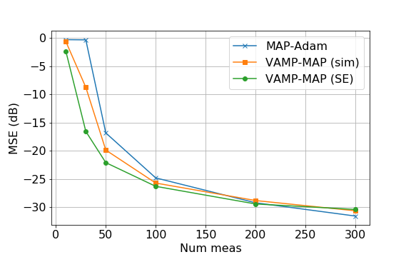
Figure 2: Normalized MSE for a random multi-layer network for (a) MAP inference computed by Adam optimizer; (b) MAP inference from ML-VAMP; (c) State evolution prediction.

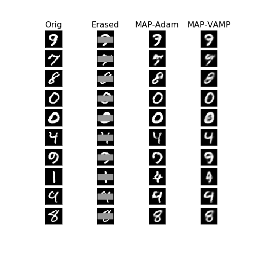
Figure 3: MNIST inpainting where the rows 10-20 of the 28 $\times$ 28 digits are erased.

Conclusions

MAP inference combined with deep generative priors provides a powerful tool for complex inverse problems. Rigorous analysis of these methods has been difficult. ML-VAMP with MAP estimation provides a computationally tractable method for performing the MAP inference with performance that can be rigorously and precisely characterized in a certain large system limit. The approach thus offers a new and potentially powerful approach for understanding and improving deep network-based inference.

Appendix A Proof of Theorem 1

The linear equalities in (13) can be rewritten as,

$$\mathbf{r}_{k\ell}^{+} =\widehat{\mathbf{z}}^{+}_{k\ell}+\frac{1}{\alpha^{-}_{k\ell}}\mathbf{s}^{+}_{k\ell}$$ (24a)

$$\mathbf{r}_{k+1,\ell}^{-} =\widehat{\mathbf{z}}^{-}_{k\ell}-\frac{1}{\alpha^{+}_{k\ell}}\mathbf{s}^{-}_{k\!+\!1,\ell}$$ (24b)

Substituting (24) in lines 10 and 20 of Algorithm 1 give the updates (14b) and (15b) in Theorem 1. It remains to show that the optimization problem in updates (14a) and (15a) is equivalent to (5). It suffices to show that the terms dependent on $(z_{\ell-1}^{-},z^{+}_{\ell})$ in both the objective functions $J_{\ell}$ from (5) and $\mathcal{L}_{\ell}$ from (14a) and (15a) are identical. This follows immediately on substituting (24) in (3).

It now suffices to show that any fixed point of Algorithm 1 is a critical point of the augmented Lagrangian in (11). Since we are looking only at fixed points, we can drop the dependence on the iteration $k$. So, for example, we can write $\mathbf{r}_{\ell}^{+}$ for $\mathbf{r}_{k\ell}^{+}$. To show that $\widehat{\mathbf{z}}^{+}_{\ell},\widehat{\mathbf{z}}^{-}_{\ell}$ are critical points of the constrained optimization (10), we need to show that there exists dual parameters $\mathbf{s}_{\ell}$ such that for all $\ell=0,\ldots,L\!-\!1$,

$$\widehat{\mathbf{z}}^{+}_{\ell}=\widehat{\mathbf{z}}^{-}_{\ell},$$ (25)

$$\frac{\partial\mathcal{L}(\widehat{\mathbf{z}}^{+},\widehat{\mathbf{z}}^{-},\mathbf{s})}{\partial\mathbf{z}^{+}_{\ell}}=0,\quad\frac{\partial\mathcal{L}(\widehat{\mathbf{z}}^{+},\widehat{\mathbf{z}}^{-},\mathbf{s})}{\partial\mathbf{z}^{-}_{\ell}}=0,$$ (26)

where $\mathcal{L}(\cdot)$ is the Lagrangian in (11).

We first prove (25) whereby primal feasibility is satisfied. At any fixed point of (7), we have

$$\eta_{\ell}=\gamma^{+}_{\ell}+\gamma^{-}_{\ell}=\frac{\gamma^{+}_{\ell}}{\alpha_{\ell}^{-}}=\frac{\gamma_{\ell}^{-}}{\alpha_{\ell}^{+}}.$$

Therefore,

$$\alpha_{\ell}^{-}=\frac{\gamma^{+}_{\ell}}{\gamma_{\ell}^{+}+\gamma_{\ell}^{-}}=1-\frac{\gamma^{-}_{\ell}}{\gamma_{\ell}^{+}+\gamma_{\ell}^{-}}=1-\alpha^{+}_{\ell}.$$ (27)

Now, from line 10 in Algorithm 1,

$$\widehat{\mathbf{z}}^{+}_{\ell} =(1-\alpha^{+}_{\ell})\mathbf{r}^{+}_{\ell}+\alpha^{+}_{\ell}\mathbf{r}^{-}_{\ell}$$

$$=\alpha^{-}_{\ell}\mathbf{r}^{+}_{\ell}+\alpha^{+}_{\ell}\mathbf{r}^{-}_{\ell},$$ (28)

where the last step used (27). Similarly, from line 20,

$$\widehat{\mathbf{z}}^{-}_{\ell}=\alpha^{-}_{\ell}\mathbf{r}^{+}_{\ell}+\alpha^{+}_{\ell}\mathbf{r}^{-}_{\ell}.$$ (29)

Equations (28) and (29) prove (25). In the sequel, we will let $\widehat{\mathbf{z}}_{\ell}$ denote $\widehat{\mathbf{z}}^{+}_{\ell}$ and $\widehat{\mathbf{z}}^{-}_{\ell}$ since they are equal. As a consequence of the primal feasibility $\widehat{\mathbf{z}}^{+}_{\ell}=\widehat{\mathbf{z}}^{-}_{\ell}$, observe that

$$\mathbf{s}_{\ell}^{+}-\mathbf{s}_{\ell}^{-}=(\alpha_{\ell}^{+}+\alpha_{\ell}^{-})\widehat{\mathbf{z}}_{\ell}-\alpha^{+}_{\ell}\mathbf{r}_{\ell}^{-}-\alpha^{-}_{\ell}\mathbf{r}_{\ell}^{+}=0,$$ (30)

where we have used (27) and (28). Define $\mathbf{s}:=\mathbf{s}^{+}=\mathbf{s}^{-}$, by virtue of the equality shown above.

Having shown the equivalence of Algorithm 1 and the iterative updates in the statement of the theorem, we can say that there exists a one-to-one linear mapping between their fixed points $\{\widehat{\mathbf{z}},\mathbf{r}^{+},\mathbf{r}^{-}\}$ (from Algorithm 1) and $\{\widehat{\mathbf{z}},\mathbf{s}\}$ (from Theorem 1). Now to show (26) it suffices to show that $\mathbf{s}_{\ell}$ is a valid dual parameter for which the following stationarity conditions hold,

$$\frac{\partial\mathcal{L}_{\ell}(\mathbf{z}^{-}_{\ell-1},\mathbf{z}^{+}_{\ell};\widehat{\mathbf{z}}^{+}_{\ell-1},\widehat{\mathbf{z}}^{-}_{\ell},\mathbf{s}_{\ell-1},\mathbf{s}_{\ell})}{\partial\mathbf{z}^{-}_{\ell-1}}\Bigg{\rvert}_{(\widehat{\mathbf{z}}_{\ell-1}^{-},\widehat{\mathbf{z}}_{\ell}^{+})}\owns\ \ {\bf 0},$$ (31)

$$\frac{\partial\mathcal{L}_{\ell}(\mathbf{z}^{-}_{\ell-1},\mathbf{z}^{+}_{\ell};\widehat{\mathbf{z}}^{+}_{\ell-1},\widehat{\mathbf{z}}^{-}_{\ell},\mathbf{s}_{\ell-1},\mathbf{s}_{\ell})}{\partial\mathbf{z}^{+}_{\ell}}\Bigg{\rvert}_{(\widehat{\mathbf{z}}_{\ell-1}^{-},\widehat{\mathbf{z}}_{\ell}^{+})}\owns\ \ {\bf 0}.$$ (32)

Indeed the above conditions are the stationarity conditions of the optimization problem in (14a) and (15a).

Appendix B Empirical Convergence of Random Variables

We follow the framework of Bayati and Montanari [31], which models various sequences as deterministic, but with components converging empirically to a distribution. We start with a brief review of useful definitions. Let $\mathbf{x}=(\mathbf{x}_{1},\ldots,\mathbf{x}_{N})$ be a block vector with components $\mathbf{x}_{n}\in{\mathbb{R}}^{r}$ for some $r$. Thus, the vector $\mathbf{x}$ is a vector with dimension $rN$. Given any function $g:{\mathbb{R}}^{r}\rightarrow{\mathbb{R}}^{s}$, we define the componentwise extension of $g(\cdot)$ as the function,

$$\mathbf{g}(\mathbf{x}):=(g(\mathbf{x}_{1}),\ldots,g(\mathbf{x}_{N}))\in{\mathbb{R}}^{Ns}.$$ (33)

That is, $\mathbf{g}(\cdot)$ applies the function $g(\cdot)$ on each $r$-dimensional component. Similarly, we say $\mathbf{g}(\mathbf{x})$ acts componentwise on $\mathbf{x}$ whenever it is of the form (33) for some function $g(\cdot)$.

Next consider a sequence of block vectors of growing dimension,

$$\mathbf{x}(N)=(\mathbf{x}_{1}(N),\ldots,\mathbf{x}_{N}(N)),\qquad N=1,\,2,\,\ldots,$$

where each component $\mathbf{x}_{n}(N)\in{\mathbb{R}}^{r}$. In this case, we will say that $\mathbf{x}(N)$ is a block vector sequence that scales with $N$ under blocks $\mathbf{x}_{n}(N)\in{\mathbb{R}}^{r}$. When $r=1$, so that the blocks are scalar, we will simply say that $\mathbf{x}(N)$ is a vector sequence that scales with $N$. Such vector sequences can be deterministic or random. In most cases, we will omit the notational dependence on $N$ and simply write $\mathbf{x}$.

Now, given $p\geq 1$, a function $f:{\mathbb{R}}^{r}\rightarrow{\mathbb{R}}^{s}$ is called pseudo-Lipschitz continuous of order $p$, if there exists a constant $C>0$ such that for all $\mathbf{x}_{1},\mathbf{x}_{2}\in{\mathbb{R}}^{r}$,

$$\|f(\mathbf{x}_{1})-f(\mathbf{x}_{2})\|\leq C\|\mathbf{x}_{1}-\mathbf{x}_{2}\|\left[1+\|\mathbf{x}_{1}\|^{p-1}+\|\mathbf{x}_{2}\|^{p-1}\right].$$

Observe that in the case $p=1$, pseudo-Lipschitz continuity reduces to the standard Lipschitz continuity. Given $p\geq 1$, we will say that the block vector sequence $\mathbf{x}=\mathbf{x}(N)$ converges empirically with $p$-th order moments if there exists a random variable $X\in{\mathbb{R}}^{r}$ such that

1. $\mathbb{E}\|X\|_{p}^{p}<\infty$; and

2. for any $f:{\mathbb{R}}^{r}\rightarrow{\mathbb{R}}$ that is pseudo-Lipschitz continuous of order $p$,

   $$\lim_{N\rightarrow\infty}\frac{1}{N}\sum_{n=1}^{N}f(\mathbf{x}_{n}(N))=\mathbb{E}\left[f(X)\right].$$ (34)

In (34), we have the empirical mean of the components $f(\mathbf{x}_{n}(N))$ of the componentwise extension $\mathbf{f}(\mathbf{x}(N))$ converging to the expectation $\mathbb{E}[f(X)]$. In this case, with some abuse of notation, we will write

$$\lim_{N\rightarrow\infty}\left\{\mathbf{x}_{n}\right\}\stackrel{{\scriptstyle PL(p)}}{{=}}X,$$ (35)

where, as usual, we have omitted the dependence on $N$ in $\mathbf{x}_{n}(N)$. Importantly, empirical convergence can de defined on deterministic vector sequences, with no need for a probability space. If $\mathbf{x}=\mathbf{x}(N)$ is a random vector sequence, we will often require that the limit (35) holds almost surely.

We conclude with one final definition. Let ${\bm{\phi}}(\mathbf{r},\gamma)$ be a function on $\mathbf{r}\in{\mathbb{R}}^{s}$ and $\gamma\in{\mathbb{R}}$. We say that ${\bm{\phi}}(\mathbf{r},\gamma)$ is uniformly Lipschitz continuous in $\mathbf{r}$ at $\gamma=\overline{\gamma}$ if there exists constants $L_{1}$ and $L_{2}\geq 0$ and an open neighborhood $U$ of $\overline{\gamma}$, such that

$$\|{\bm{\phi}}(\mathbf{r}_{1},\gamma)-{\bm{\phi}}(\mathbf{r}_{2},\gamma)\|\leq L_{1}\|\mathbf{r}_{1}-\mathbf{r}_{2}\|,$$ (36)

for all $\mathbf{r}_{1},\mathbf{r}_{2}\in{\mathbb{R}}^{s}$ and $\gamma\in U$; and

$$\|{\bm{\phi}}(\mathbf{r},\gamma_{1})-{\bm{\phi}}(\mathbf{r},\gamma_{2})\|\leq L_{2}\left(1+\|\mathbf{r}\|\right)|\gamma_{1}-\gamma_{2}|,$$ (37)

for all $\mathbf{r}\in{\mathbb{R}}^{s}$ and $\gamma_{1},\gamma_{2}\in U$.

Appendix C Large System Limit: Model Details

In addition to the assumptions in Section IV, we describe a few more technical assumptions. First, we need that the activation functions ${\bm{\phi}}_{\ell}(z_{\ell\!-\!1},\xi_{\ell})$ in (1b) act componentwise meaning that,

$$\left[{\bm{\phi}}_{\ell}(\mathbf{z}_{\ell\!-\!1},{\bm{\xi}}_{\ell})\right]_{n}=\phi_{\ell}(z_{\ell\!-\!1,n},\xi_{\ell,n})$$ (38)

for some scalar-valued function $\phi_{\ell}(\cdot)$ for all components $n$. That is, for a nonlinear layer $\ell=2,4,\ldots,L$, each output $z^{0}_{\ell,n}$ depends only on the corresponding input component $z^{0}_{\ell\!-\!1,n}$. Standard activations such as ReLU or sigmoid would satisfy this property. In addition, we require that the activation function components $\phi_{\ell}(\cdot)$ are pseudo-Lipschitz continuous of order two.

Next, we need certain assumptions on the estimation functions $\mathbf{g}_{\ell}^{\pm}(\cdot)$. For the estimation functions corresponding to the nonlinear layers, $\ell=2,4,\ldots,L-2$, we assume that for each parameter $\theta_{k\ell}^{-}$, the function $\mathbf{g}_{\ell}^{+}(\mathbf{r}_{\ell\!-\!1}^{+},\mathbf{r}_{\ell}^{-},\theta_{\ell}^{-})$ is Lipschitz continuous in $(\mathbf{r}^{+}_{\ell\!-\!1},\mathbf{r}^{-}_{\ell})$ and $\mathbf{g}^{+}_{\ell}(\cdot)$ acts componentwise in that,

$$\widehat{\mathbf{z}}^{+}_{\ell}=\mathbf{g}_{\ell}^{+}(\mathbf{r}^{+}_{\ell\!-\!1},\mathbf{r}^{-}_{\ell},\theta_{\ell}^{+})\Leftrightarrow\widehat{z}^{+}_{\ell,i}=g_{\ell}^{+}(r^{+}_{\ell\!-\!1,i},r^{-}_{\ell,i},\theta_{\ell}^{+}),$$ (39)

for $i=1,\ldots,N_{\ell}$. for some scalar-valued function $g_{\ell}^{+}(\cdot)$. Thus, each element $\widehat{z}^{+}_{\ell,i}$ of the output vector $\widehat{\mathbf{z}}^{+}_{\ell}$ depends only the corresponding elements of the inputs $r^{+}_{\ell\!-\!1,i}$ and $r^{-}_{\ell,i}$. We make a similar assumption on the first estimation function $\mathbf{g}^{+}_{0}(\cdot)$ as well as the reverse functions $\mathbf{g}^{-}_{\ell}(\cdot)$ for $\ell=2,4,\ldots,L$ and define $g_{0}^{+}(\cdot)$ and $g_{\ell}^{-}(\cdot)$ in a similar manner.

Note that for the linear layers $\ell=1,3,\ldots,L\!-\!1$, we assume the MAP denoiser (4). For the linear layer, this is identical to the MMSE denoiser and the estimation functions can be written as,

$$\mathbf{g}^{+}_{\ell}(\mathbf{r}^{+}_{\ell\!-\!1},\mathbf{r}^{-}_{\ell\!-\!1},\theta^{+}_{\ell})$$

$$=\mathbf{V}_{\ell}{\mathbf{G}}^{+}_{\ell}(\mathbf{V}_{\ell\!-\!1}\mathbf{r}^{+}_{\ell\!-\!1},\mathbf{V}_{\ell}^{\text{\sf T}}\mathbf{r}^{-}_{\ell\!-\!1},\bar{\mathbf{s}}_{\ell},\bar{\mathbf{b}}_{\ell},\theta^{-}_{\ell})$$ (40a)

$$\mathbf{g}^{-}_{\ell}(\mathbf{r}^{+}_{\ell\!-\!1},\mathbf{r}^{-}_{\ell\!-\!1},\theta^{+}_{\ell})$$

$$:=\mathbf{V}_{\ell\!-\!1}^{\text{\sf T}}{\mathbf{G}}^{+}_{\ell}(\mathbf{V}_{\ell\!-\!1}\mathbf{r}^{+}_{\ell\!-\!1},\mathbf{V}_{\ell}^{\text{\sf T}}\mathbf{r}^{-}_{\ell\!-\!1},\bar{\mathbf{s}}_{\ell},\bar{\mathbf{b}}_{\ell},\theta^{-}_{\ell}),$$ (40b)

where, for each parameter value $\theta^{\pm}_{\ell}$, the functions ${\mathbf{G}}^{\pm}_{\ell}(\cdot)$ are Lipschitz continuous in $(\mathbf{r}^{+}_{\ell\!-\!1},\mathbf{r}^{-}_{\ell},\bar{\mathbf{s}}_{\ell})$ and are componentwise extensions of ${G}_{\ell}^{\pm}$ defined as,

$$\begin{bmatrix}{G}_{\ell}^{-}(\bar{u}_{\ell\!-\!1},\bar{u}_{\ell},s_{\ell},\bar{b}_{\ell},\gamma_{\ell\!-\!1}^{+},\gamma_{\ell}^{-})\\ {G}_{\ell}^{+}(\bar{u}_{\ell\!-\!1},\bar{u}_{\ell},s_{\ell},\bar{b}_{\ell},\gamma_{\ell\!-\!1}^{+},\gamma_{\ell}^{-})\end{bmatrix}$$

$$=\begin{bmatrix}\gamma_{\ell\!-\!1}^{+}+\nu_{\ell}s_{\ell}^{2}&-\nu_{\ell}s_{\ell}\\ -\nu_{\ell}s_{\ell}&\gamma_{\ell}^{-}+\nu_{\ell}\end{bmatrix}^{-1}\begin{bmatrix}\gamma_{\ell\!-\!1}^{+}\bar{u}_{\ell\!-\!1}-\nu_{\ell}s_{\ell}\bar{b}_{\ell}\\ \gamma_{\ell}^{-}\bar{u}_{\ell}+\nu_{\ell}\bar{b}_{\ell}\end{bmatrix},$$ (41)

We call the functions ${\mathbf{G}}^{\pm}_{\ell}(\cdot)$, the transformed denoising functions. We refer the reader to the appendices of [30] for a detailed derivation of $\mathbf{G}^{\pm}_{\ell}$. We now need two further technical assumptions.

Algorithm 2 Transformed ML-VAMP Recursion

1:  // Initialization

2:  Initial vectors $\mathbf{w}_{\ell}$, $\mathbf{q}^{0}_{0}$, $\mathbf{q}_{0\ell}^{-}$

3:  $\mathbf{q}^{0}_{0}=\mathbf{f}^{0}_{0}(\mathbf{w}_{0}),\quad\mathbf{p}^{0}_{0}=\mathbf{V}_{0}\mathbf{q}^{0}_{0}$

4:  for $\ell=1,\ldots,L\!-\!1$ do

5:     $\mathbf{q}^{0}_{\ell}=\mathbf{f}^{0}_{\ell}(\mathbf{p}^{0}_{\ell\!-\!1},\mathbf{w}_{\ell},\Lambda_{01}^{-})$

6:     $\mathbf{p}^{0}_{\ell}=\mathbf{V}_{\ell}\mathbf{q}^{0}_{\ell}$

7:  end for

8:  

9:  for $k=0,1,\dots,N_{\rm it}-1$ do

10:     // Forward Pass

11:     $\widehat{\mathbf{q}}^{+}_{k0}=\mathbf{h}^{+}_{0}(\mathbf{q}^{-}_{k\ell},\mathbf{w}_{\ell},\theta^{+}_{k0})$

12:     $\alpha^{+}_{k0}={\langle\partial\mathbf{h}^{+}_{0}(\mathbf{q}^{-}_{k0},\mathbf{w}_{\ell},\theta^{+}_{k0})/\partial\mathbf{q}^{-}_{k0}\rangle}$

13:     $\Lambda_{k0}^{+}=(\alpha_{k0}^{+},\theta_{k0}^{+})$

14:     $\mathbf{q}^{+}_{k0}=\mathbf{f}^{+}_{0}(\mathbf{q}^{-}_{k0},\mathbf{w}_{\ell},\Lambda^{+}_{k0})$

15:     $\mathbf{p}^{+}_{k0}=\mathbf{V}_{0}\mathbf{q}^{+}_{k0}$

16:     for $\ell=1,\ldots,L\!-\!1$ do

17:        $\widehat{\mathbf{q}}^{+}_{k\ell}=\mathbf{h}^{+}_{\ell}(\mathbf{p}^{0}_{\ell\!-\!1},\mathbf{p}^{+}_{k,\ell\!-\!1},\mathbf{q}^{-}_{k\ell},\mathbf{w}_{\ell},\theta^{+}_{k\ell})$

18:        $\alpha^{+}_{k\ell}={\langle\partial\mathbf{h}^{+}_{\ell}(\mathbf{p}^{+}_{k,\ell\!-\!1},\mathbf{q}^{-}_{k\ell},\mathbf{w}_{\ell},\theta^{+}_{k\ell})/\partial\mathbf{q}^{-}_{k\ell}\rangle}$

19:        $\Lambda_{k\ell}^{+}=(\alpha_{k\ell}^{+},\theta_{k\ell}^{+})$

20:        $\mathbf{q}^{+}_{k\ell}=\mathbf{f}^{+}_{\ell}(\mathbf{p}^{+}_{k,\ell\!-\!1},\mathbf{q}^{-}_{k\ell},\mathbf{w}_{\ell},\Lambda^{+}_{k\ell})$

21:        $\mathbf{p}^{+}_{k\ell}=\mathbf{V}_{\ell}\mathbf{q}^{+}_{k\ell}$

22:     end for

23:     

24:     // Reverse Pass

25:     $\widehat{\mathbf{p}}^{-}_{k\!+\!1,L\!-\!1}=\mathbf{h}^{-}_{L}(\mathbf{p}^{+}_{k,L\!-\!1},\mathbf{w}_{L},\theta^{-}_{kL})$

26:     $\alpha^{-}_{k,L\!-\!1}={\langle\partial\mathbf{h}^{-}_{L}(\mathbf{p}^{+}_{k,L\!-\!1},\mathbf{w}_{L},\theta^{-}_{kL})/\partial\mathbf{p}^{+}_{k,L\!-\!1}\rangle}$

27:     $\Lambda_{kL}^{-}=(\alpha_{k,L\!-\!1}^{-},\theta_{kL}^{-})$

28:     $\mathbf{p}^{-}_{k\!+\!1,L\!-\!1}=\mathbf{f}^{-}_{L}(\mathbf{p}^{+}_{k,L\!-\!1},\mathbf{w}_{L},\Lambda^{-}_{kL})$

29:     for $\ell=L-2,\ldots,0$ do

30:        $\widehat{\mathbf{p}}^{-}_{k\!+\!1,\ell\!-\!1}=\mathbf{h}^{-}_{\ell\!+\!1}(\mathbf{p}^{+}_{k\ell},\mathbf{q}^{-}_{k,\ell\!+\!1},\mathbf{w}_{\ell\!+\!1},\theta^{-}_{k,\ell\!+\!1})$

31:        $\alpha^{-}_{k\ell}={\langle\partial\mathbf{h}^{-}_{\ell\!+\!1}(\mathbf{p}^{+}_{k\ell},\cdots)/\partial\mathbf{p}^{+}_{k\ell}\rangle}$

32:        $\Lambda_{k,\ell\!+\!1}^{-}=(\alpha_{k,\ell\!+\!1}^{-},\theta_{k,\ell\!+\!1}^{-})$

33:        $\mathbf{p}^{-}_{k\!+\!1,\ell}=\mathbf{f}^{-}_{\ell\!+\!1}(\mathbf{p}^{+}_{k\ell},\mathbf{q}^{-}_{k,\ell\!+\!1},\mathbf{w}_{\ell\!+\!1},\Lambda^{-}_{k,\ell\!+\!1})$

34:        $\mathbf{q}^{-}_{k\!+\!1,\ell}=\mathbf{V}_{\ell}^{\text{\sf T}}\mathbf{p}^{-}_{k\!+\!1,\ell}$

35:     end for

36:  end for

Algorithm 3 State Evolution for ML-VAMP

0:  Vector update component functions $f^{0}_{\ell}(\cdot)$ and $f^{\pm}_{k\ell}(\cdot)$

1:  

2:  // Initial pass

3:  Initial random variables: $W_{\ell}$, $Q_{0\ell}^{-}$, $\ell=0,\ldots,L\!-\!1$

4:  $Q^{0}_{0}=f^{0}_{0}(W_{0})$

5:  $P^{0}_{0}\sim{\mathcal{N}}(0,\tau^{0}_{0})$, $\tau^{0}_{0}=\mathbb{E}(Q^{0}_{0})^{2}$

6:  for $\ell=1,\ldots,L\!-\!1$ do

7:     $Q^{0}_{\ell}=f^{0}_{\ell}(P^{0}_{\ell\!-\!1},W_{\ell})$

8:     $P^{0}_{\ell}={\mathcal{N}}(0,\tau^{0}_{\ell})$, $\tau^{0}_{\ell}=\mathbb{E}(Q^{0}_{\ell})^{2}$

9:  end for

10:  

11:  for $k=0,1,\dots$ do

12:     // Forward Pass

13:     $\widehat{Q}^{+}_{k0}=h^{+}_{0}(Q_{k0}^{-},W_{0},\theta^{+}_{k0}))$

14:     $\overline{\alpha}_{k0}^{+}=\mathbb{E}(\partial h^{+}_{0}(Q_{k0}^{-},W_{0},\theta^{+}_{k0})/\partial Q_{k0}^{-})$

15:     $\overline{\Lambda}_{k0}^{+}=(\overline{\alpha}^{+}_{k0},\theta_{k0}^{+})$

16:     $Q_{k0}^{+}=f^{+}_{k0}(Q_{k0}^{-},W_{0},\overline{\Lambda}^{+}_{k0})$

17:     $(P^{0}_{0},P_{k0}^{+})={\mathcal{N}}(\mathbf{0},\mathbf{K}_{k0}^{+})$, $\mathbf{K}_{k0}^{+}=\mathrm{Cov}(Q^{0}_{0},Q_{k0}^{+})$

18:     for $\ell=1,\ldots,L-1$ do

19:        $\widehat{Q}^{+}_{k\ell}=h^{+}_{\ell}(P^{0}_{\ell\!-\!1},P^{+}_{k,\ell\!-\!1},Q_{k\ell}^{-},W_{\ell},\theta^{+}_{k\ell}))$

20:        $\overline{\alpha}_{k0}^{+}=\mathbb{E}(\partial h^{+}_{\ell}(\ldots))/\partial Q_{k\ell}^{-})$

21:        $\overline{\Lambda}_{k\ell}^{+}=(\overline{\alpha}^{+}_{k\ell},\theta_{k\ell}^{+})$

22:        $Q_{k\ell}^{+}=f^{+}_{k\ell}(P^{0}_{\ell\!-\!1},P^{+}_{k,\ell\!-\!1},Q_{k\ell}^{-},W_{\ell},\overline{\Lambda}^{+}_{k\ell})$

23:        $(P^{0}_{\ell},P_{k\ell}^{+})={\mathcal{N}}(\mathbf{0},\mathbf{K}_{k\ell}^{+})$, $\mathbf{K}_{k\ell}^{+}=\mathrm{Cov}(Q^{0}_{\ell},Q_{k\ell}^{+})$

24:     end for

25:     

26:     // Reverse Pass

27:     $\widehat{P}_{k\!+\!1,L\!-\!1}^{-}=h^{-}_{kL}(P^{0}_{L\!-\!1},P_{k,L\!-\!1}^{+},W_{L},\theta^{-}_{k\!+\!1,L})$

28:     $\overline{\alpha}_{k,L\!-\!1}^{-}=\partial h^{-}_{kL}(\cdots)/\partial P_{k,L\!-\!1}^{+}$

29:     $\overline{\Lambda}_{k,L\!-\!1}^{-}=(\overline{\alpha}^{-}_{k,L\!-\!1},\theta_{k,L\!-\!1}^{-})$

30:     $P_{k\!+\!1,L\!-\!1}^{-}=f^{-}_{kL}(P^{0}_{L\!-\!1},P_{k,L\!-\!1}^{+},W_{L},\overline{\Lambda}^{-}_{k\!+\!1,L})$

31:     $\tau_{k\!+\!1,L\!-\!1}^{-}=\mathbb{E}(P^{-}_{k\!+\!1,L\!-\!1})^{2}$

32:     $Q_{k\!+\!1,L\!-\!1}^{-}={\mathcal{N}}(0,\tau_{k\!+\!1,L\!-\!1}^{-})$

33:     for $\ell=L\!-\!1,\ldots,1$ do

34:        $\widehat{P}_{k\!+\!1,\ell\!-\!1}^{-}=h^{-}_{k\ell}(P^{0}_{\ell\!-\!1},P_{k,\ell\!-\!1}^{+},W_{\ell},\theta^{-}_{k\!+\!1,\ell})$

35:        $\overline{\alpha}_{k,\ell\!-\!1}^{-}=\mathbb{E}(\partial h^{-}_{k\ell}(\ldots)/\partial P_{k,L\!-\!1}^{+})$

36:        $\overline{\Lambda}_{k\ell}^{-}=(\overline{\alpha}^{-}_{k,\ell\!-\!1},\theta_{k,\ell}^{-})$

37:        $P_{k\!+\!1,\ell\!-\!1}^{-}=f^{-}_{k\ell}(P^{0}_{\ell\!-\!1},P^{+}_{k,\ell\!-\!1},Q_{k\!+\!1,\ell}^{-},W_{\ell},\overline{\Lambda}^{-}_{k\ell})$

38:        $\tau_{k\!+\!1,\ell\!-\!1}^{-}=\mathbb{E}(P_{k\!+\!1,\ell\!-\!1}^{-})^{2}$

39:        $Q_{k\!+\!1,\ell\!-\!1}^{-}={\mathcal{N}}(0,\tau_{k\!+\!1,\ell\!-\!1}^{-})$

40:     end for

41:  end for

Appendix D Proof of Theorem 2

D-A Transformed MLP

The SE analysis of MMSE ML-VAMP in [30] proves a result on a general class of multi-layer recursions, called Gen-ML. To prove Theorem 2, we will show that ML-VAMP algorithm in Algorithm 1 is of the form of an almost identical recursion with some minor changes in notation. Theorem 2 in this paper will then follow from applying the general result in [30]. Since most of the proof is identical, we highlight only the main differences.

Similar to [30], we rewrite the MLP in (1) in a certain transformed form. To this end, define the disturbance vectors,

$$\mathbf{w}_{0} :=\widehat{\mathbf{z}}^{0}_{0},\quad\mathbf{w}_{\ell}:={\bm{\xi}}_{\ell},\quad\ell=2,4,\ldots,L$$ (42a)

$$\mathbf{w}_{\ell} =(\bar{\mathbf{s}}_{\ell},\bar{\mathbf{b}}_{\ell},\bar{{\bm{\xi}}}_{\ell}),\quad\ell=1,3,\ldots,L\!-\!1.$$ (42b)

Also, define the scalar-valued functions,

$$f^{0}_{0}(w_{0}):=w_{0},$$ (43a)

$$f^{0}_{\ell}(p^{0}_{\ell\!-\!1},w_{\ell})=f^{0}_{\ell}(p^{0}_{\ell\!-\!1},\xi_{\ell}):=\phi_{\ell}(p^{0}_{\ell\!-\!1},\xi_{\ell}),$$

$$\ell=2,4,\ldots,L$$ (43b)

$$f^{0}_{\ell}(p^{0}_{\ell\!-\!1},w_{\ell})=f^{0}_{\ell}(p^{0}_{\ell\!-\!1},(\bar{s}_{\ell},\bar{b}_{\ell},\bar{\xi}_{\ell}))=\bar{s}_{\ell}p^{0}_{\ell}+\bar{b}_{\ell}+\bar{\xi}_{\ell},$$

$$\ell=1,3,\ldots,L\!-\!1.$$ (43c)

Let $\mathbf{f}^{0}_{\ell}(\cdot)$ be their componentwise extension, meaning that

$$\left[\mathbf{f}^{0}_{\ell}(\mathbf{p}^{0}_{\ell\!-\!1,n},\mathbf{w}_{\ell,n})\right]_{n}:=f^{0}_{\ell}(p^{0}_{\ell\!-\!1,n},w_{\ell,n}),$$

so that $\mathbf{f}^{0}_{\ell}(\cdot)$ acts with the scalar-valued function $f^{0}_{\ell}(\cdot)$ on each component of the vectors. With this definition, it is shown in [30] that the vectors $\mathbf{p}^{0}_{\ell}$ and $\mathbf{q}^{0}_{\ell}$ satisfy the recursions in “Initialization" section of Algorithm 2, the transformed algorithm. This system of equations is represented diagrammatically in the top panel of Fig. 4. In comparison to Fig. 1, the transforms $\mathbf{W}_{\ell}$ of the linear layers have been expanded using the SVD $\mathbf{W}_{\ell}=\mathbf{V}_{\ell}{\bm{\Sigma}}_{\ell}\mathbf{V}_{\ell\!-\!1}$ and inserting intermediate variables $\mathbf{q}^{0}_{\ell}$ and $\mathbf{p}^{0}_{\ell}$. With the transformation, the MLP (1) is equivalent to a sequence of linear transforms by orthogonal matrices $\mathbf{V}_{\ell}$ and non-linear componentwise mappings $f^{0}_{\ell}(\cdot)$.

Figure 4: Transformed view of the MLP and message passing system in Fig. 1. The linear transforms $\mathbf{W}_{\ell}$ are replaced by the SVD $\mathbf{W}_{\ell}=\mathbf{V}_{\ell}{\bm{\Sigma}}_{\ell}\mathbf{V}_{\ell\!-\!1}$, and intermediate layers are added for each component of the SVD. With this transformation, the MLP and message passing algorithm are reduced to alternating multiplications by $\mathbf{V}_{\ell}$ and $\mathbf{V}_{\ell}^{*}$ and componentwise (possibly nonlinear) functions.

D-B Parameters

To handle parameterized functions, the analysis in [30] introduces the concept of parameter lists. For our purpose, let

$$\Lambda^{+}_{k\ell}:=(\alpha_{k\ell}^{+},\theta_{k\ell}^{+}),\quad\Lambda^{-}_{k\ell}:=(\alpha_{k\ell}^{-},\theta_{k\ell}^{-}),$$ (44)

which is simply the parameter $\alpha_{k\ell}^{\pm}$ along with the parameter $\theta_{k\ell}^{\pm}$ for the estimators.

D-C Estimation Functions

Similar to the transformed system in the top panel of Fig. 4, we next represent the steps in the ML-VAMP Algorithm 1 as a sequence of alternating linear and nonlinear maps. Let $\ell=0,2,4,\ldots,L$ be the index of a nonlinear layer and define the scalar-valued functions,

$$h^{+}_{0}(q_{0}^{-},w_{0},\theta_{k0}^{+}):=g^{+}_{0}(q^{-}_{0}+w_{0},\theta_{k0}^{+}),$$ (45a)

$$h^{+}_{\ell}(p^{0}_{\ell\!-\!1},p_{\ell\!-\!1}^{+},q_{\ell}^{-},w_{\ell},\theta_{k\ell}^{+})$$

$$:=g^{+}_{\ell}(p_{\ell\!-\!1}^{+}+p^{0}_{\ell\!-\!1},q^{-}_{\ell}+q^{0}_{\ell},\theta_{k\ell}^{+}),$$ (45b)

$$h^{-}_{L}(p^{0}_{L\!-\!1},p_{L\!-\!1}^{+},w_{L},\theta_{k,L}^{-}):=g^{-}_{L}(p_{L\!-\!1}^{+}+p^{0}_{L\!-\!1},\theta_{k,L}^{-}).$$ (45c)

$$h^{-}_{\ell}(p^{0}_{\ell\!-\!1},p_{\ell\!-\!1}^{+},q_{\ell}^{-},w_{\ell},\theta_{k,\ell\!+\!1}^{+})$$

$$:=g^{-}_{\ell}(p_{\ell\!-\!1}^{+}+p^{0}_{\ell\!-\!1},q^{-}_{\ell}+q^{0}_{\ell},\theta_{k\ell}^{-}),$$ (45d)

For $\ell=1,3,\ldots,L\!-\!1$, the index of a linear layer, and $w_{\ell}=(\bar{s}_{\ell},\bar{b}_{\ell})$, let

$$h^{+}_{\ell}(p_{\ell\!-\!1}^{0},p_{\ell\!-\!1}^{+},q_{\ell}^{-},w_{\ell},\theta_{k\ell}^{+})$$

$$:=G^{+}_{\ell}(p_{\ell\!-\!1}^{+}+p^{0}_{\ell\!-\!1},q^{-}_{\ell}+q^{0}_{\ell},\bar{s}_{\ell},\bar{b}_{\ell},\theta^{+}_{k\ell}),$$ (46a)

$$h^{-}_{\ell}(p_{\ell\!-\!1}^{0},p_{\ell\!-\!1}^{+},q_{\ell}^{-},w_{\ell},\theta_{k\ell}^{-})$$

$$:=G^{-}_{\ell}(p_{\ell\!-\!1}^{+}+p^{0}_{\ell\!-\!1},q^{-}_{\ell}+q^{0}_{\ell},\bar{s}_{\ell},\bar{b}_{\ell},\theta^{-}_{k\ell}),$$ (46b)

where $G^{\pm}(\cdot)$ are the components of the transformed linear estimation functions. For both the linear and nonlinear layers, we then define the update functions as,

$$f^{+}_{0}(q_{0}^{-},w_{0},\Lambda_{k0}^{+}):=\frac{1}{1-\alpha_{k\ell}^{+}}$$

$$\times\left[h^{+}_{0}(q_{0}^{-},w_{0},\theta_{k0}^{+})-w_{0}-\alpha_{k0}^{+}q_{0}^{-}\right],$$ (47a)

$$f^{+}_{\ell}(p^{0}_{\ell\!-\!1},p_{\ell\!-\!1}^{+},q_{\ell}^{-},w_{\ell},\Lambda_{k\ell}^{+}):=\frac{1}{1-\alpha_{k\ell}^{+}}$$

$$\times\left[h^{+}_{\ell}(p^{0}_{\ell\!-\!1},p_{\ell\!-\!1}^{+},q_{\ell}^{-},w_{\ell},\theta_{k\ell}^{+})-q^{0}_{\ell}-\alpha_{k\ell}^{+}Q_{\ell}^{-}\right],$$ (47b)

$$f^{-}_{L}(p^{0}_{L\!-\!1},p_{L\!-\!1}^{+},w_{L},\Lambda_{kL}^{-}):=\frac{1}{1-\alpha_{k\ell}^{-}}$$

$$\times\left[h^{-}_{L}(p^{0}_{L\!-\!1},p_{L\!-\!1}^{+},w_{L},\theta_{kL}^{-})-p^{0}_{L\!-\!1}-\alpha_{k,L\!-\!1}^{-}p_{L\!-\!1}^{+}\right],$$ (47c)

$$f^{-}_{\ell}(p^{0}_{\ell\!-\!1},p_{\ell\!-\!1}^{+},q_{\ell}^{-},w_{\ell},\Lambda_{k\ell}^{-}):=\frac{1}{1-\alpha_{k,\ell\!-\!1}^{-}}$$

$$\times\left[h^{-}_{\ell}(p^{0}_{\ell\!-\!1},p_{\ell\!-\!1}^{+},q_{\ell}^{-},w_{\ell},\theta_{k\ell}^{-})-p^{0}_{\ell\!-\!1}-\alpha_{k,\ell\!-\!1}^{-}p_{\ell\!-\!1}^{+}\right].$$ (47d)

With these definitions, let $\mathbf{f}^{\pm}_{\ell}(\cdot)$ and $\mathbf{h}^{\pm}_{\ell}(\cdot)$ be the componentwise extensions of $f^{\pm}_{\ell}(\cdot)$ and $h^{\pm}_{\ell}(\cdot)$. It is then shown in [30] that the vectors in (22) satisfy the recursions in the “Forward" and “Reverse" passes of the transformed ML recursion in Algorithm 2.

This is diagrammatically represented in the bottom panel of Fig. 4. We see that, in the forward pass, the vectors are generated by an alternating sequence of componentwise mappings where

$$\mathbf{q}^{+}_{k\ell}=\mathbf{f}^{+}_{\ell}(\mathbf{p}^{+}_{k,\ell\!-\!1},\mathbf{q}^{-}_{k\ell},\cdots),$$

followed by multiplication by $\mathbf{V}_{\ell}$,

$$\mathbf{p}^{+}_{k\ell}=\mathbf{V}_{\ell}\mathbf{q}^{+}_{k\ell}.$$

Similarly, in the reverse pass, we have a componentwise mapping,

$$\mathbf{p}^{-}_{k\ell}=\mathbf{f}^{-}_{\ell\!+\!1}(\mathbf{p}^{+}_{k\ell},\mathbf{q}^{-}_{k,\ell\!+\!1},\cdots),$$

followed by multiplication by $\mathbf{V}_{\ell}^{\text{\sf T}}$,

$$\mathbf{q}^{-}_{k\ell}=\mathbf{V}_{\ell}^{\text{\sf T}}\mathbf{p}^{-}_{k\ell}.$$

Thus, similar to the MLP, we have written the forward and reverse passes of the multi-layer updates as alternating sequence of componentwise (possibly nonlinear) functions followed by multiplications by orthogonal matrices.

D-D SE Analysis

Now that the variables and the ML-VAMP algorithm estiamtes are written in the form of Algorithm (2), the analysis of [30] to derive a simple state evolution. Let

$$W_{0} :=Z^{0}_{0},\quad W_{\ell}:=\Xi_{\ell},\quad\ell=2,4,\ldots,L$$ (48a)

$$W_{\ell} =(\bar{S}_{\ell},\bar{B}_{\ell},\bar{\Xi}_{\ell}),\quad\ell=1,3,\ldots,L\!-\!1,$$ (48b)

where $Z^{0}_{0}$, $\Xi_{\ell}$ and $(\bar{S}_{\ell},\bar{B}_{\ell},\bar{\Xi}_{\ell})$ are the random variable limits in (18) and (20). With these definitions, we can recursively define the random variables $Q_{k\ell}^{\pm}$ and $P_{k\ell}^{\pm}$ from the steps in Algorithm 3. This recursive definition of random variables is called the state evolution. We see that the SE updates in Algorithm 3 are in a one-to-one correspondence with the steps in Transformed ML-VAMP algorithm, Algorithm 2. The key difference is that the SE updates involves scalar random variables, as opposed to vectors. The random variables are all either Gaussian random variables or the output of nonlinear function of the Gaussian random variables. In addition, the parameters of the Gaussians such as $\mathbf{K}^{+}_{k\ell}$ and $\tau^{-}_{k\ell}$ are fully deterministic since they are computed via expectations.

We now make further assumption:

Assumption 1.

Let $\overline{\alpha}_{k\ell}^{\pm}$ be generated by the SE recursions in Algorithm 3. Then $\overline{\alpha}^{\pm}_{k\ell}\in(0,1)$ from the for all $k$ and $\ell$.

We can now state the main result. The result includes Theorem 2 as a special case.

Theorem 3.

Let $\mathbf{w}_{\ell},\mathbf{p}^{\pm}_{k\ell}$, $\mathbf{q}^{\pm}_{k\ell}$, $\mathbf{p}^{0}_{\ell}$, $\mathbf{q}^{0}_{\ell}$ be defined as above. Consider the sequence of random variables defined by the SE updates in Algorithm 3 under the above assumptions. Then,

1. For any fixed $k$ and $\ell=1,\ldots,L\!-\!1$, the parameter list $\Lambda_{k\ell}^{+}$ converges as

   $$\lim_{N\rightarrow\infty}\Lambda_{k\ell}^{+}=\overline{\Lambda}_{k\ell}^{+}$$ (49)

   almost surely. Also, the components of $\mathbf{w}_{\ell}$, $\mathbf{p}^{0}_{\ell\!-\!1}$, $\mathbf{q}^{0}_{\ell}$, $\mathbf{p}_{0,\ell\!-\!1}^{+},\ldots,\mathbf{p}_{k,\ell\!-\!1}^{+}$ and $\mathbf{q}_{0\ell}^{\pm},\ldots,\mathbf{q}_{k\ell}^{\pm}$ almost surely empirically converge jointly with limits,

   $$\lim_{N\rightarrow\infty}\left\{(p^{0}_{\ell\!-\!1,n},p^{+}_{i,\ell\!-\!1,n},q^{0}_{\ell,n},q^{-}_{j\ell,n},q^{+}_{j\ell,n})\right\}$$

   $$=(P^{0}_{\ell\!-\!1},P^{+}_{i,\ell\!-\!1},Q^{0}_{\ell},Q^{-}_{j\ell},Q^{+}_{j\ell}),$$ (50)

   for all $i,j=0,\ldots,k$, where the variables $P^{0}_{\ell\!-\!1}$, $P_{i,\ell\!-\!1}^{+}$ and $Q_{j\ell}^{-}$ are zero-mean jointly Gaussian random variables independent of $W_{\ell}$ with

   $$\begin{split}&\mathrm{Cov}(P^{0}_{\ell\!-\!1},P_{i,\ell\!-\!1}^{+})=\mathbf{K}_{i,\ell\!-\!1}^{+},\quad\mathbb{E}(Q_{j\ell}^{-})^{2}=\tau_{j\ell}^{-},\\ &\mathbb{E}(P_{i,\ell\!-\!1}^{+}Q_{j\ell}^{-})=0,\quad\mathbb{E}(P^{0}_{\ell\!-\!1}Q_{j\ell}^{-})=0,\end{split}$$

   The identical result holds for $\ell=0$ with the variables $\mathbf{p}_{i,\ell\!-\!1}^{+}$ and $P_{i,\ell\!-\!1}^{+}$ removed.

2. For any fixed $k>0$ and $\ell=1,\ldots,L\!-\!1$, the parameter lists $\Lambda_{k\ell}^{-}$ converge as

   $$\lim_{N\rightarrow\infty}\Lambda_{k\ell}^{-}=\overline{\Lambda}_{k\ell}^{-}$$ (51)

   almost surely. Also, the components of $\mathbf{w}_{\ell}$, $\mathbf{p}^{0}_{\ell\!-\!1}$, $\mathbf{p}_{0,\ell\!-\!1}^{+},\ldots,\mathbf{p}_{k\!-\!1,\ell\!-\!1}^{+}$, $\mathbf{p}_{0,\ell\!-\!1}^{+},\ldots,\mathbf{p}_{k\!-\!1,\ell\!-\!1}^{+}$, and $\mathbf{q}_{0\ell}^{-},\ldots,\mathbf{q}_{k\ell}^{-}$ almost surely empirically converge jointly with limits,

   $$\lim_{N\rightarrow\infty}\left\{(p^{0}_{\ell\!-\!1,n},p^{+}_{i,\ell\!-\!1,n},q^{-}_{j\ell,n},q^{+}_{j\ell,n})\right\}$$

   $$=(P^{0}_{\ell\!-\!1},P^{+}_{i,\ell\!-\!1},Q^{-}_{j\ell},Q^{+}_{j\ell}),$$ (52)

   for all $i=0,\ldots,k\!-\!1$ and $j=0,\ldots,k$, where the variables $P^{0}_{\ell\!-\!1}$, $P_{i,\ell\!-\!1}^{+}$ and $Q_{j\ell}^{-}$ are zero-mean jointly Gaussian random variables independent of $W_{\ell}$ with

   $$\begin{split}&\mathrm{Cov}(P^{0}_{\ell\!-\!1},P_{i,\ell\!-\!1}^{+})=\mathbf{K}_{i,\ell\!-\!1}^{+},\quad\quad\mathbb{E}(Q_{j\ell}^{-})^{2}=\tau_{j\ell}^{-},\\ &\mathbb{E}(P_{i,\ell\!-\!1}^{+}Q_{j\ell}^{-})=0,\quad\mathbb{E}(P^{0}_{\ell\!-\!1}Q_{j\ell}^{-})=0,\end{split}$$ (53)

   The identical result holds for $\ell=L$ with all the variables $\mathbf{q}_{j\ell}^{-}$ and $Q_{j\ell}^{-}$ removed. Also, for $k=0$, we remove the variables with $\mathbf{p}_{k\!-\!1,\ell}^{+}$ and $P_{k\!-\!1,\ell}^{+}$.

Proof.

This is proven almost identically to the result in [30]. $\Box$

Appendix E Numerical Experiments Details

Synthetic random network

The simulation is identical to [30], except that we have run MAP ML-VAMP intead of MMSE ML-VAMP. The details of the simulation are as follows: As described in Section V, the network input is a $N_{0}=20$ dimensional Gaussian unit noise vector $\mathbf{z}_{0}$. and has three hidden layers with 100 and 500 units and a variable number $N_{y}$ of output units. For the weight matrices and bias vectors in all but the final layer, we took $\mathbf{W}_{\ell}$ and $\mathbf{b}_{\ell}$ to be random i.i.d. Gaussians. The mean of the bias vector was selected so that only a fixed fraction, $\rho=0.4$, of the linear outputs would be positive. The activation functions were rectified linear units (ReLUs), $\phi_{\ell}(z)=\max\{0,x\}$. Hence, after activation, there would be only a fraction $\rho=0.4$ of the units would be non-zero. In the final layer, we constructed the matrix similar to [34] where $\mathbf{A}=\mathbf{U}\mathrm{Diag}(\mathbf{s})\mathbf{V}^{\text{\sf T}}$, with $\mathbf{U}$ and $\mathbf{V}$ be random orthogonal matrices and $\mathbf{s}$ be logarithmically spaced valued to obtain a desired condition number of $\kappa=10$. It is known from [34] that matrices with high condition numbers are precisely the matrices in which AMP algorithms fail. For the linear measurements, $\mathbf{y}=\mathbf{A}\mathbf{z}_{5}+\mathbf{w}$, the noise level $10\log_{10}(\mathbb{E}\|\mathbf{w}\|^{2}/\|\mathbf{A}\mathbf{z}_{5}\|^{2})$ is set at 30 dB. In Fig. 2, we have plotted the normalized MSE (in dB) which we define as

$$\mathrm{NMSE}:=10\log_{10}\left[\frac{\|\mathbf{z}^{0}_{0}-\widehat{\mathbf{z}}^{\pm}_{k0}\|^{2}}{\|\mathbf{z}^{0}_{0}\|^{2}}\right].$$

Since each iteration of ML-VAMP involves a forward and reverse pass, we say that each iteration consists of two “half-iterations", using the same terminology as turbo codes. The left panel of Fig. 2 plots the NMSE vs. half iterations.

MNIST inpainting

The well-known MNIST dataset consists of handwritten images of size $28\times 28=784$ pixels. We followed the procedure in [2] for training a generative model from 50,000 digits. Each image $\mathbf{x}$ is modeled as the output of a neural network input dimension of 20 variables followed by a single hidden layer with 400 units and an output layer of 784 units, corresponding to the dimension of the digits. ReLUs were used for activation functions and a sigmoid was placed at the output to bound the final pixel values between 0 and 1. The inputs $\mathbf{z}^{0}_{0}$ were the modeled as zero mean Gaussians with unit variance. The data was trained using the Adam optimizer with the default parameters in TensorFlow The training optimization was run with 20,000 steps with a batch size of 100 corresponding to 40 epochs.

The ML-VAMP algorithm was compared against MAP estimation. As studied in [5, 6], MAP estimation can be performed via numerical minimization of the likelihood. In this study, We used TensorFlow for the minimization. We found the fastest convergence with the Adam optimizer at a step-size of 0.01. This required only 500 iterations to be within 1% of the final loss function. For MAP ML-VAMP, the sigmoid function does not have an analytic denoiser, so it was approximated with a probit output. We found that the basic MAP ML-VAMP algorithm could be unstable. Hence, damping as described in [34] and [18] was used. With damping, we needed to run the ML-VAMP algorithm for up to 500 iterations, which is comparable to the Adam optimizer.

References

[1]
D. J. Rezende, S. Mohamed, and D. Wierstra, “Stochastic backpropagation and
approximate inference in deep generative models,” in Proc. ICML,
2014, pp. 1278–1286.
[2]
D. P. Kingma and M. Welling, “Auto-encoding variational bayes,”
arXiv:1312.6114, 2013.
[3]
A. Radford, L. Metz, and S. Chintala, “Unsupervised representation learning
with deep convolutional generative adversarial networks,” arXiv
preprint arXiv:1511.06434, 2015.
[4]
R. Salakhutdinov, “Learning deep generative models,” Annual Review of
Statistics and Its Application, vol. 2, pp. 361–385, 2015.
[5]
R. Yeh, C. Chen, T. Y. Lim, M. Hasegawa-Johnson, and M. N. Do, “Semantic image
inpainting with perceptual and contextual losses,” arXiv:1607.07539,
2016.
[6]
A. Bora, A. Jalal, E. Price, and A. G. Dimakis, “Compressed sensing using
generative models,” Proc. ICML, 2017.
[7]
J. R. Chang, C.-L. Li, B. Poczos, and B. V. Kumar, “One network to solve them
all—solving linear inverse problems using deep projection models,” in
2017 IEEE International Conference on Computer Vision (ICCV). IEEE, 2017, pp. 5889–5898.
[8]
A. Mousavi, A. B. Patel, and R. G. Baraniuk, “A deep learning approach to
structured signal recovery,” in Proc. IEEE Allerton Conference,
2015, pp. 1336–1343.
[9]
C. Metzler, A. Mousavi, and R. Baraniuk, “Learned D-amp: Principled neural
network based compressive image recovery,” in Proc. NIPS, 2017, pp.
1772–1783.
[10]
M. Borgerding, P. Schniter, and S. Rangan, “AMP-inspired deep networks for
sparse linear inverse problems,” IEEE Transactions on Signal
Processing, vol. 65, no. 16, pp. 4293–4308, 2017.
[11]
P. Hand and V. Voroninski, “Global guarantees for enforcing deep generative
priors by empirical risk,” arXiv preprint arXiv:1705.07576, 2017.
[12]
V. Shah and C. Hegde, “Solving linear inverse problems using gan priors: An
algorithm with provable guarantees,” arXiv preprint arXiv:1802.08406,
2018.
[13]
D. L. Donoho, A. Maleki, and A. Montanari, “Message-passing algorithms for
compressed sensing,” PNAS, vol. 106, no. 45, pp. 18 914–18 919,
Nov. 2009.
[14]
A. Manoel, F. Krzakala, M. Mézard, and L. Zdeborová, “Multi-layer
generalized linear estimation,” arXiv:1701.06981, 2017.
[15]
A. K. Fletcher, S. Rangan, and P. Schniter, “Inference in deep networks in
high dimensions,” Proc. IEEE ISIT, 2018.
[16]
M. Gabrié, A. Manoel, C. Luneau, J. Barbier, N. Macris, F. Krzakala, and
L. Zdeborová, “Entropy and mutual information in models of deep neural
networks,” in Proc. NIPS, 2018.
[17]
G. Reeves, “Additivity of information in multilayer networks via additive
gaussian noise transforms,” arXiv preprint arXiv:1710.04580, 2017.
[18]
S. Rangan, P. Schniter, and A. K. Fletcher, “Vector approximate message
passing,” in Proc. IEEE ISIT, 2017, pp. 1588–1592.
[19]
J. Ma and L. Ping, “Orthogonal AMP,” IEEE Access, vol. 5, pp.
2020–2033, 2017.
[20]
K. Takeuchi, “Rigorous dynamics of expectation-propagation-based signal
recovery from unitarily invariant measurements,” in Proc. IEEE ISIT,
2017, pp. 501–505.
[21]
T. P. Minka, “Expectation propagation for approximate bayesian inference,” in
Proc. Uncertainty in artificial intelligence, 2001, pp. 362–369.
[22]
M. Opper and O. Winther, “Expectation consistent approximate inference,”
Journal of Machine Learning Research, vol. 6, no. Dec, pp. 2177–2204,
2005.
[23]
B. Cakmak, O. Winther, and B. H. Fleury, “S-AMP: Approximate message passing
for general matrix ensembles,” in Proc. IEEE ITW, 2014.
[24]
S. Boyd, N. Parikh, E. Chu, B. Peleato, J. Eckstein et al.,
“Distributed optimization and statistical learning via the alternating
direction method of multipliers,” Foundations and
Trends® in Machine learning, vol. 3, no. 1, pp. 1–122,
2011.
[25]
S. Rangan, P. Schniter, E. Riegler, A. K. Fletcher, and V. Cevher, “Fixed
points of generalized approximate message passing with arbitrary matrices,”
IEEE Trans. Info. Theory, vol. 62, no. 12, pp. 7464–7474, 2016.
[26]
S. Rangan, A. K. Fletcher, P. Schniter, and U. S. Kamilov, “Inference for
generalized linear models via alternating directions and Bethe free energy
minimization,” IEEE Trans. Info. Theory, vol. 63, no. 1, pp.
676–697, 2017.
[27]
A. Manoel, F. Krzakala, G. Varoquaux, B. Thirion, and L. Zdeborová,
“Approximate message-passing for convex optimization with non-separable
penalties,” arXiv preprint arXiv:1809.06304, 2018.
[28]
B. He, H. Liu, J. Lu, and X. Yuan, “Application of the strictly contractive
peaceman-rachford splitting method to multi-block separable convex
programming,” in Splitting Methods in Communication, Imaging, Science,
and Engineering. Springer, 2016, pp.
195–235.
[29]
D. Han and X. Yuan, “Convergence analysis of the peaceman-rachford splitting
method for nonsmooth convex optimization,” J. Optim. Theory
Appl.,(Under-revision), vol. 1, 2012.
[30]
A. K. Fletcher, S. Rangan, and P. Schniter, “Inference in deep networks in
high dimensions,” arXiv preprint arXiv:1706.06549, 2017.
[31]
M. Bayati and A. Montanari, “The dynamics of message passing on dense graphs,
with applications to compressed sensing,” IEEE Trans. Info. Theory,
vol. 57, no. 2, pp. 764–785, Feb. 2011.
[32]
D. P. Kingma and J. Ba, “Adam: A method for stochastic optimization,”
arXiv preprint arXiv:1412.6980, 2014.
[33]
P. Pandit, M. Sahraee, S. Rangan, and A. K. Fletcher, “Asymptotics of MAP
inference in deep networks,” arxiv preprint, 2019.
[34]
S. Rangan, P. Schniter, and A. K. Fletcher, “On the convergence of approximate
message passing with arbitrary matrices,” in Proc. IEEE ISIT, Jul.
2014, pp. 236–240.