Β 

Bernoulli Race Particle Filters


Β 


Sebastian M Schmon Β Β Β Β Β Β Β Β Β Β Β Β Β Β Β Β Β Β Β Β Β Β  Arnaud Doucet Β Β Β Β Β Β Β Β Β Β Β Β Β Β Β Β Β Β Β Β Β Β  George Deligiannidis

Department of Statistics University of Oxford Β Β Β Β Β Β Β Β Β Β Β Β Β Β Β Β Β Β Β Β Β Β  Department of Statistics University of Oxford Β Β Β Β Β Β Β Β Β Β Β Β Β Β Β Β Β Β Β Β Β Β  Department of Statistics University of Oxford

Abstract

When the weights in a particle filter are not available analytically, standard resampling methods cannot be employed. To circumvent this problem state-of-the-art algorithms replace the true weights with non-negative unbiased estimates. This algorithm is still valid but at the cost of higher variance of the resulting filtering estimates in comparison to a particle filter using the true weights. We propose here a novel algorithm that allows for resampling according to the true intractable weights when only an unbiased estimator of the weights is available. We demonstrate our algorithm on several examples.

Keywords: Bernoulli factory, random weight particle filter, unbiased estimation, Rao-Blackwellization

Introduction

Over the last 25 years particle filters have become a standard tool for optimal estimation in the context of general state space hidden Markov models (HMMs) with applications in ever more complex scenarios. HMMs are described by a latent (unobserved) process (Xt)tβˆˆβ„•subscriptsubscript𝑋𝑑𝑑ℕ(X_{t})_{t\in\mathbb{N}} taking values in a space 𝖷𝖷\mathsf{X} and evolving according to the state transition density

Xt∣(Xtβˆ’1=x)∼f(β‹…βˆ£x)X_{t}\mid(X_{t-1}=x)\sim f(\,\cdot\mid x)

for tβ‰₯2𝑑2t\geq 2 and X1βˆΌΞΌβ€‹(β‹…)similar-tosubscript𝑋1πœ‡β‹…X_{1}\sim\mu(\cdot). The states can be observed through an observation process (Yt)tβˆˆβ„•subscriptsubscriptπ‘Œπ‘‘π‘‘β„•(Y_{t})_{t\in\mathbb{N}}, taking values in a space 𝖸𝖸\mathsf{Y} with observation density

Yt∣(Xt=x)∼g(β‹…βˆ£x).Y_{t}\mid(X_{t}=x)\sim g(\,\cdot\mid x).

Particle filters (PFs) sequentially approximate the joint distributions

Ο€t​(x1:t)subscriptπœ‹π‘‘subscriptπ‘₯:1𝑑\displaystyle\pi_{t}\left(x_{1:t}\right) =p​(x1:t∣y1:t)absent𝑝conditionalsubscriptπ‘₯:1𝑑subscript𝑦:1𝑑\displaystyle=p(x_{1:t}\mid y_{1:t})
=g​(y1∣x1)​μ​(x1)β€‹βˆk=2tg​(yk∣xk)​f​(xk∣xkβˆ’1)p​(y1:t)absent𝑔conditionalsubscript𝑦1subscriptπ‘₯1πœ‡subscriptπ‘₯1superscriptsubscriptproductπ‘˜2𝑑𝑔conditionalsubscriptπ‘¦π‘˜subscriptπ‘₯π‘˜π‘“conditionalsubscriptπ‘₯π‘˜subscriptπ‘₯π‘˜1𝑝subscript𝑦:1𝑑\displaystyle=\frac{g(y_{1}\mid x_{1})\mu(x_{1})\prod_{k=2}^{t}g(y_{k}\mid x_{k})f(x_{k}\mid x_{k-1})}{p(y_{1:t})}
=g​(y1∣x1)​μ​(x1)β€‹βˆk=2tϖ​(xk∣yk,xkβˆ’1)p​(y1:t)absent𝑔conditionalsubscript𝑦1subscriptπ‘₯1πœ‡subscriptπ‘₯1superscriptsubscriptproductπ‘˜2𝑑italic-Ο–conditionalsubscriptπ‘₯π‘˜subscriptπ‘¦π‘˜subscriptπ‘₯π‘˜1𝑝subscript𝑦:1𝑑\displaystyle=\frac{g(y_{1}\mid x_{1})\mu(x_{1})\prod_{k=2}^{t}\varpi\left(x_{k}\mid y_{k},x_{k-1}\right)}{p(y_{1:t})}

on the space 𝖷tsuperscript𝖷𝑑\mathsf{X}^{t} at time t𝑑t by evolving a set of samples, termed particles, through time. We use here the shorthand notation xj:k=(xj,…,xk)subscriptπ‘₯:π‘—π‘˜subscriptπ‘₯𝑗…subscriptπ‘₯π‘˜x_{j:k}=(x_{j},\ldots,x_{k}). The quantity p​(y1:t)𝑝subscript𝑦:1𝑑p(y_{1:t}) denotes the marginal likelihood of the model

p​(y1:t)=∫g​(y1∣x1)​μ​(x1)β€‹βˆk=2tϖ​(xk∣yk,xkβˆ’1)​d​x1:t𝑝subscript𝑦:1𝑑𝑔conditionalsubscript𝑦1subscriptπ‘₯1πœ‡subscriptπ‘₯1superscriptsubscriptproductπ‘˜2𝑑italic-Ο–conditionalsubscriptπ‘₯π‘˜subscriptπ‘¦π‘˜subscriptπ‘₯π‘˜1𝑑subscriptπ‘₯:1𝑑p(y_{1:t})=\int g(y_{1}\mid x_{1})\mu(x_{1})\prod_{k=2}^{t}\varpi\left(x_{k}\mid y_{k},x_{k-1}\right)dx_{1:t} (1)

which is usually intractable. The PF algorithm proceeds as follows. Given a set of particles {Xtβˆ’1i,i=1,…,N}formulae-sequencesuperscriptsubscript𝑋𝑑1𝑖𝑖1…𝑁\{X_{t-1}^{i},i=1,\ldots,N\} at time tβˆ’1𝑑1t-1 the particles are propagated through q​(xt∣xtβˆ’1,yt)π‘žconditionalsubscriptπ‘₯𝑑subscriptπ‘₯𝑑1subscript𝑦𝑑q(x_{t}\mid x_{t-1},y_{t}). To adjust for the discrepancy between the distribution of the proposed states and Ο€t​(x1:t)subscriptπœ‹π‘‘subscriptπ‘₯:1𝑑\pi_{t}\left(x_{1:t}\right) the particles are weighted by

wt​(xtβˆ’1,xt)subscript𝑀𝑑subscriptπ‘₯𝑑1subscriptπ‘₯𝑑\displaystyle w_{t}(x_{t-1},x_{t}) =ϖ​(xt∣yt,xtβˆ’1)q​(xt∣xtβˆ’1,yt),tβ‰₯2,formulae-sequenceabsentitalic-Ο–conditionalsubscriptπ‘₯𝑑subscript𝑦𝑑subscriptπ‘₯𝑑1π‘žconditionalsubscriptπ‘₯𝑑subscriptπ‘₯𝑑1subscript𝑦𝑑𝑑2\displaystyle=\frac{\varpi\left(x_{t}\mid y_{t},x_{t-1}\right)}{q(x_{t}\mid x_{t-1},y_{t})},\quad t\geq 2, (2)
w1​(x1)subscript𝑀1subscriptπ‘₯1\displaystyle w_{1}(x_{1}) =g​(y1∣x1)​μ​(x1)q​(x1∣y1).absent𝑔conditionalsubscript𝑦1subscriptπ‘₯1πœ‡subscriptπ‘₯1π‘žconditionalsubscriptπ‘₯1subscript𝑦1\displaystyle=\frac{g(y_{1}\mid x_{1})\mu(x_{1})}{q(x_{1}\mid y_{1})}.

A subsequent resampling step according to these weights ensures that only promising particles survive. Here we consider only multinomial resampling, where we write I1:N∼Mult​{N;w1,…,wN}similar-tosubscript𝐼:1𝑁Mult𝑁subscript𝑀1…subscript𝑀𝑁I_{1:N}\sim\textsf{Mult}\left\{N;w_{1},\ldots,w_{N}\right\} to denote the vector I1:Nsubscript𝐼:1𝑁I_{1:N} consisting of N𝑁N samples from a multinomial distribution with probabilities proportional to w1,…,wNsubscript𝑀1…subscript𝑀𝑁w_{1},\ldots,w_{N}. The algorithm is summarized in AlgorithmΒ 1.

Algorithm 1 Particle filter with N𝑁N particles
1:At time t=1𝑑1t=1
2:Sample X~1i∼q(β‹…βˆ£y1),i=1…N\widetilde{X}_{1}^{i}\sim q(\cdot\mid y_{1}),\quad i=1\ldots N
3:Compute weights
w1,i=wt​(X~1i),i=1,…,Nformulae-sequencesubscript𝑀1𝑖subscript𝑀𝑑superscriptsubscript~𝑋1𝑖𝑖1…𝑁w_{1,i}=w_{t}(\widetilde{X}_{1}^{i}),\quad i=1,\ldots,N
4:I1:N∼Mult​{N;w1,1,…,w1,N}similar-tosubscript𝐼:1𝑁Mult𝑁subscript𝑀11…subscript𝑀1𝑁I_{1:N}\sim\textsf{Mult}\left\{N;w_{1,1},\ldots,w_{1,N}\right\}
5:Set X1i=X~1Ii,i=1.…,Nformulae-sequenceformulae-sequencesuperscriptsubscript𝑋1𝑖superscriptsubscript~𝑋1subscript𝐼𝑖𝑖1…𝑁X_{1}^{i}=\widetilde{X}_{1}^{I_{i}},\quad i=1.\ldots,N
6:At times tβ‰₯2𝑑2t\geq 2
7:Sample X~ti∼q(β‹…βˆ£Xtβˆ’1i,yt),i=1,…,N\widetilde{X}_{t}^{i}\sim q(\,\cdot\mid X_{t-1}^{i},y_{t}),\quad i=1,\ldots,N
8:Compute weights as in (2)
wt,i=wt​(Xtβˆ’1i,X~ti),i=1,…,Nformulae-sequencesubscript𝑀𝑑𝑖subscript𝑀𝑑superscriptsubscript𝑋𝑑1𝑖superscriptsubscript~𝑋𝑑𝑖𝑖1…𝑁w_{t,i}=w_{t}(X_{t-1}^{i},\widetilde{X}_{t}^{i}),\quad i=1,\ldots,N
9:I1:N∼Mult​{N;wt,1,…,wt,N}similar-tosubscript𝐼:1𝑁Mult𝑁subscript𝑀𝑑1…subscript𝑀𝑑𝑁I_{1:N}\sim\textsf{Mult}\{N;w_{t,1},\ldots,w_{t,N}\}
10:For i=1,…,N𝑖1…𝑁i=1,\ldots,N set
X1:tisuperscriptsubscript𝑋:1𝑑𝑖\displaystyle X_{1:t}^{i} =(X1:(tβˆ’1)Ii,X~tIi).absentsuperscriptsubscript𝑋:1𝑑1subscript𝐼𝑖superscriptsubscript~𝑋𝑑subscript𝐼𝑖\displaystyle=\left(X_{1:(t-1)}^{I_{i}},\widetilde{X}_{t}^{I_{i}}\right).

In most applications, interest lies not in the distribution itself, but rather in the expectations

ℐ​(h)=∫h​(x1:t)​πt​(x1:t)​𝑑x1:tβ„β„Žβ„Žsubscriptπ‘₯:1𝑑subscriptπœ‹π‘‘subscriptπ‘₯:1𝑑differential-dsubscriptπ‘₯:1𝑑\mathcal{I}(h)=\int h(x_{1:t})\pi_{t}(x_{1:t})dx_{1:t} (3)

for some test function h:𝖷t→ℝ:β„Žβ†’superscript𝖷𝑑ℝh\colon\mathsf{X}^{t}\rightarrow\mathbb{R}. Applying a PF we can estimate this integral, for a set of particle genealogies {X1:ti,i=1,…,N}formulae-sequencesuperscriptsubscript𝑋:1𝑑𝑖𝑖1…𝑁\left\{X_{1:t}^{i},i=1,\ldots,N\right\}, by taking

ℐ^t,PF​(h)=1Nβ€‹βˆ‘i=1Nh​(X1:ti).subscript^ℐ𝑑PFβ„Ž1𝑁superscriptsubscript𝑖1π‘β„Žsuperscriptsubscript𝑋:1𝑑𝑖\widehat{\mathcal{I}}_{t,\mathrm{PF}}(h)=\frac{1}{N}\sum_{i=1}^{N}h\left(X_{1:t}^{i}\right). (4)

When the PF weights (2) are not available analytically, standard resampling routinesβ€”steps 3 and 7 in AlgorithmΒ 1β€”cannot be performed. However, in many cases one might be able to construct an unbiased estimator of the resampling weights. [liu1998sequential, rousset2006discussion, DelMoral2007, fearnhead2008particle] show that using random but unbiased non-negative weights still yields a valid algorithm. This can be easily seen by considering a standard particle filter on an extended space. Yet, this flexibility does not come without cost. Replacing the true weights with a noisy estimate increases the variance for Monte Carlo estimates of type (4).

Here we introduce a new resampling scheme that allows for multinomial resampling from the true intractable weights while just requiring access to non-negative unbiased estimates. Thus, any PF estimate of type (4) will have the same variance as if the true weights were known. This algorithm relies on an extension of recent work in [dughmi2017bernoulli] where the authors consider an unrelated problem.

In the supplementary material we collect the proofs for Propositions 3, 4 and 5, Theorem 6 and additional simulation studies. Code to reproduce our results is available online111URL: http://www.stats.ox.ac.uk/~schmon/..

1 Particle Filters with Intractable Weights

Particle filters for state space models with intractable weights rely on the observation that replacing the true weights with a non-negative unbiased estimate is equivalent to a particle filter on an extended space. In this section we introduce some examples of models where the weights are indeed not available analytically and review briefly how the random weight particle filter (RWPF) can be applied in these instances.

1.1 Locally optimal proposal

Recall that in the setting of a PF for a state space model at time tβˆ’1𝑑1t-1 the proposal for t𝑑t which leads to the minimum one step variance, termed the locally optimal proposal qβˆ—superscriptπ‘žq^{*}, is

qβˆ—β€‹(xt∣xtβˆ’1,yt)=g​(yt∣xt)​f​(xt∣xtβˆ’1)p​(yt∣xtβˆ’1),superscriptπ‘žconditionalsubscriptπ‘₯𝑑subscriptπ‘₯𝑑1subscript𝑦𝑑𝑔conditionalsubscript𝑦𝑑subscriptπ‘₯𝑑𝑓conditionalsubscriptπ‘₯𝑑subscriptπ‘₯𝑑1𝑝conditionalsubscript𝑦𝑑subscriptπ‘₯𝑑1q^{*}(x_{t}\mid x_{t-1},y_{t})=\frac{g(y_{t}\mid x_{t})f(x_{t}\mid x_{t-1})}{p(y_{t}\mid x_{t-1})},

see, e.g. [doucet2000sequential, Proposition 2]. Sampling from the locally optimal proposal is usually straightforward using a rejection sampler. The weights

wt​(xtβˆ’1,xt)subscript𝑀𝑑subscriptπ‘₯𝑑1subscriptπ‘₯𝑑\displaystyle w_{t}(x_{t-1},x_{t}) =p​(yt∣xtβˆ’1)absent𝑝conditionalsubscript𝑦𝑑subscriptπ‘₯𝑑1\displaystyle=p(y_{t}\mid x_{t-1})
=∫g​(yt∣xt)​f​(xt∣xtβˆ’1)​𝑑xt,absent𝑔conditionalsubscript𝑦𝑑subscriptπ‘₯𝑑𝑓conditionalsubscriptπ‘₯𝑑subscriptπ‘₯𝑑1differential-dsubscriptπ‘₯𝑑\displaystyle=\int g(y_{t}\mid x_{t})f(x_{t}\mid x_{t-1})dx_{t}, (5)

however, are intractable if the integral on the right-hand side does not have an analytical expression, thus prohibiting an exact implementation of this algorithm. Our algorithm will enable us to resample according to these weights.

1.2 Partially observed diffusions

Most research on particle filters with intractable weights has been carried out in the setting of partially observed diffusions, see e.g. [fearnhead2008particle], which we will describe here briefly. For simplicity, consider the univariate diffusion222It is not necessary to restrict oneself to univariate diffusions, see e.g. [fearnhead2008particle]. process of the form

d​Xt=a​(Xt)​d​t+d​Bt,t∈[0,𝒯],formulae-sequence𝑑subscriptπ‘‹π‘‘π‘Žsubscript𝑋𝑑𝑑𝑑𝑑subscript𝐡𝑑𝑑0𝒯dX_{t}=a(X_{t})dt+dB_{t},\quad t\in[0,\mathcal{T}], (6)

where a:ℝ→ℝ:π‘Žβ†’β„β„a\colon\mathbb{R}\rightarrow\mathbb{R} denotes the drift function and π’―βˆˆβ„π’―β„\mathcal{T}\in\mathbb{R} is the time horizon. For a general diffusion constant speed as assumed in (6) can be obtained whenever the Lamperti transform is available. The diffusion is observed at discrete times ti,i=1,…​Tformulae-sequencesubscript𝑑𝑖𝑖1…𝑇t_{i},i=1,\ldots T with measurement error described by the density g​(yti∣xti)𝑔conditionalsubscript𝑦subscript𝑑𝑖subscriptπ‘₯subscript𝑑𝑖g(y_{t_{i}}\mid x_{t_{i}}). In this model the resampling weights are often intractable since for most diffusion processes the transition density fΔ​t​(xti∣xtiβˆ’1)subscript𝑓Δ𝑑conditionalsubscriptπ‘₯subscript𝑑𝑖subscriptπ‘₯subscript𝑑𝑖1f_{\Delta t}(x_{t_{i}}\mid x_{t_{i-1}}) over the interval with length Δ​t=tiβˆ’tiβˆ’1Δ𝑑subscript𝑑𝑖subscript𝑑𝑖1\Delta t=t_{i}-t_{i-1} is not available analytically. However, as shown in [rogers1985smooth, dacunha1986estimation, beskos2005exact] the transition density over an interval of length Δ​tΔ𝑑\Delta t can be expressed as

fΔ​t​(y∣x)subscript𝑓Δ𝑑conditional𝑦π‘₯\displaystyle f_{\Delta t}(y\mid x) =φ​(y;x,Δ​t)​exp⁑(A​(y)βˆ’A​(x))absentπœ‘π‘¦π‘₯Δ𝑑𝐴𝑦𝐴π‘₯\displaystyle=\varphi(y;x,\Delta t)\exp\left(A(y)-A(x)\right)
×𝔼​[exp⁑(βˆ’βˆ«0Δ​tϕ​(Ws)​𝑑s)]absent𝔼delimited-[]superscriptsubscript0Δ𝑑italic-Ο•subscriptπ‘Šπ‘ differential-d𝑠\displaystyle\quad\times\mathbb{E}\left[\exp\left(-\int_{0}^{\Delta t}\phi(W_{s})ds\right)\right] (7)

where φ​(β‹…;x,Δ​t)πœ‘β‹…π‘₯Δ𝑑\varphi(\,\cdot\,;x,\Delta t) is the density of a Normal distribution with mean xπ‘₯x and variance Δ​tΔ𝑑\Delta t, (Ws)s∈[0,Δ​t]subscriptsubscriptπ‘Šπ‘ π‘ 0Δ𝑑\left(W_{s}\right)_{s\in[0,\Delta t]} denotes a Brownian bridge from xπ‘₯x to y𝑦y and ϕ​(x)=(a2​(x)+a′​(x))/2italic-Ο•π‘₯superscriptπ‘Ž2π‘₯superscriptπ‘Žβ€²π‘₯2\phi(x)=\left(a^{2}(x)+a^{\prime}(x)\right)/2 for a function A:ℝ→ℝ:𝐴→ℝℝA\colon\mathbb{R}\rightarrow\mathbb{R} with A′​(x)=a​(x)superscript𝐴′π‘₯π‘Žπ‘₯A^{\prime}(x)=a(x). The expectation on the right-hand side in (7) is with respect to the Brownian bridge and is usually intractable. Thus, for a particle filter to work in this example one either needs to implement a Bootstrap PF, which can sample the diffusion (6) exactly [beskos2005exact, see, e.g.], or one constructs an unbiased estimator of the expectation on the right-hand side to employ the RWPF. Note that for a function g𝑔g and U∼Unif​[0,t]similar-toπ‘ˆUnif0𝑑U\sim\mathrm{Unif}[0,t] we have

𝔼​[g​(WU)λ∣Ws,0≀s≀t]=∫0tg​(Ws)λ​t​𝑑s.𝔼delimited-[]conditional𝑔subscriptπ‘Šπ‘ˆπœ†subscriptπ‘Šπ‘ 0𝑠𝑑superscriptsubscript0𝑑𝑔subscriptπ‘Šπ‘ πœ†π‘‘differential-d𝑠\mathbb{E}\left[\frac{g(W_{U})}{\lambda}\mid W_{s},0\leq s\leq t\right]=\int_{0}^{t}\frac{g(W_{s})}{\lambda t}ds.

Using this relationship we can use debiasing schemes such as the Poisson estimator [Beskos2006] to find a non-negative unbiased estimator of the expectation of the exponential.

1.3 Random weight particle filter

Here we briefly review the RWPF and compare its asymptotic variance to that of a PF with known weights. Assume one does not have access to the weight ϖ​(xt∣yt,xtβˆ’1)italic-Ο–conditionalsubscriptπ‘₯𝑑subscript𝑦𝑑subscriptπ‘₯𝑑1\varpi\left(x_{t}\mid y_{t},x_{t-1}\right) in (2) but only to some non-negative unbiased estimate Ο–^​(xt∣yt,xtβˆ’1,Ut)^italic-Ο–conditionalsubscriptπ‘₯𝑑subscript𝑦𝑑subscriptπ‘₯𝑑1subscriptπ‘ˆπ‘‘\hat{\varpi}(x_{t}\mid y_{t},x_{t-1},U_{t}), where Utsubscriptπ‘ˆπ‘‘U_{t} are auxiliary variables sampled from some density mπ‘šm. Then we carry out the multinomial resampling in AlgorithmΒ 1 by taking I1:N∼Mult​{N;w^t,1,…,w^t,N}similar-tosubscript𝐼:1𝑁Mult𝑁subscript^𝑀𝑑1…subscript^𝑀𝑑𝑁I_{1:N}\sim\textsf{Mult}\{N;\hat{w}_{t,1},\ldots,\hat{w}_{t,N}\}, where w^t,ksubscript^π‘€π‘‘π‘˜\hat{w}_{t,k} is defined as in (2) with ϖ​(xt∣yt,xtβˆ’1)italic-Ο–conditionalsubscriptπ‘₯𝑑subscript𝑦𝑑subscriptπ‘₯𝑑1\varpi\left(x_{t}\mid y_{t},x_{t-1}\right) replaced by Ο–^​(xt∣yt,xtβˆ’1,Ut)^italic-Ο–conditionalsubscriptπ‘₯𝑑subscript𝑦𝑑subscriptπ‘₯𝑑1subscriptπ‘ˆπ‘‘\hat{\varpi}(x_{t}\mid y_{t},x_{t-1},U_{t}). This is equivalent to a standard particle filter on the extended space targeting at time t𝑑t the distribution

π¯t​(x1:t,u1:t)∝∏k=1tΟ–^​(xk∣yk,xkβˆ’1,uk)​m​(uk)proportional-tosubscriptΒ―πœ‹π‘‘subscriptπ‘₯:1𝑑subscript𝑒:1𝑑superscriptsubscriptproductπ‘˜1𝑑^italic-Ο–conditionalsubscriptπ‘₯π‘˜subscriptπ‘¦π‘˜subscriptπ‘₯π‘˜1subscriptπ‘’π‘˜π‘šsubscriptπ‘’π‘˜\bar{\pi}_{t}\left(x_{1:t},u_{1:t}\right)\propto\prod_{k=1}^{t}\hat{\varpi}(x_{k}\mid y_{k},x_{k-1},u_{k})m\left(u_{k}\right)

which satisfies

π¯t​(x1:t,u1:t)=Ο€t​(x1:t)​π¯t​(u1:t∣x1:t)subscriptΒ―πœ‹π‘‘subscriptπ‘₯:1𝑑subscript𝑒:1𝑑subscriptπœ‹π‘‘subscriptπ‘₯:1𝑑subscriptΒ―πœ‹π‘‘conditionalsubscript𝑒:1𝑑subscriptπ‘₯:1𝑑\bar{\pi}_{t}\left(x_{1:t},u_{1:t}\right)=\pi_{t}(x_{1:t})\bar{\pi}_{t}(u_{1:t}\mid x_{1:t}) (8)

with

π¯t​(u1:t∣x1:t)=∏k=1tΟ–^​(xk∣yk,xkβˆ’1,uk)​m​(uk)ϖ​(xk∣yk,xkβˆ’1).subscriptΒ―πœ‹π‘‘conditionalsubscript𝑒:1𝑑subscriptπ‘₯:1𝑑superscriptsubscriptproductπ‘˜1𝑑^italic-Ο–conditionalsubscriptπ‘₯π‘˜subscriptπ‘¦π‘˜subscriptπ‘₯π‘˜1subscriptπ‘’π‘˜π‘šsubscriptπ‘’π‘˜italic-Ο–conditionalsubscriptπ‘₯π‘˜subscriptπ‘¦π‘˜subscriptπ‘₯π‘˜1\bar{\pi}_{t}(u_{1:t}\mid x_{1:t})=\prod_{k=1}^{t}\frac{\hat{\varpi}(x_{k}\mid y_{k},x_{k-1},u_{k})m\left(u_{k}\right)}{\varpi\left(x_{k}\mid y_{k},x_{k-1}\right)}.

A PF targeting the sequence of distributions Ο€tsubscriptπœ‹π‘‘\pi_{t} directly can be interpreted as a Rao-Blackwellized PF [doucet2000sequential] of the PF on the extended space. Hence, the following is a direct consequence of [chopin2004central].

Proposition 1.

For any sufficiently regular333We refer the reader to [chopin2004central] for the mathematical details. real-valued test function hβ„Žh, the exact weight PF (EWPF) and RWPF estimators of ℐ​(h)β„β„Ž\mathcal{I}(h) defined in (3) both satisfy a N𝑁\sqrt{N}-central limit theorem with asymptotic variances satisfying ΟƒEWPF,h2≀σRWPF,h2superscriptsubscript𝜎EWPFβ„Ž2superscriptsubscript𝜎RWPFβ„Ž2\sigma_{\text{EWPF},h}^{2}\leq\sigma_{\text{RWPF},h}^{2}.

2 Bernoulli Races

Assume now that the intractable weights can be written as follows

wt​(xtβˆ’1,xt)=g​(yt∣xt)​f​(xt∣xtβˆ’1)q​(xt∣xtβˆ’1,yt)subscript𝑀𝑑subscriptπ‘₯𝑑1subscriptπ‘₯𝑑𝑔conditionalsubscript𝑦𝑑subscriptπ‘₯𝑑𝑓conditionalsubscriptπ‘₯𝑑subscriptπ‘₯𝑑1π‘žconditionalsubscriptπ‘₯𝑑subscriptπ‘₯𝑑1subscript𝑦𝑑\displaystyle w_{t}(x_{t-1},x_{t})=\frac{g(y_{t}\mid x_{t})f\left(x_{t}\mid x_{t-1}\right)}{q\left(x_{t}\mid x_{t-1},y_{t}\right)}
=c​(xtβˆ’1,xt,yt)​b​(xtβˆ’1,xt,yt),absent𝑐subscriptπ‘₯𝑑1subscriptπ‘₯𝑑subscript𝑦𝑑𝑏subscriptπ‘₯𝑑1subscriptπ‘₯𝑑subscript𝑦𝑑\displaystyle=c\left(x_{t-1},x_{t},y_{t}\right)b\left(x_{t-1},x_{t},y_{t}\right), (9)

where 0≀b​(x,xβ€²,y)≀10𝑏π‘₯superscriptπ‘₯′𝑦10\leq b(x,x^{\prime},y)\leq 1 for all x,xβ€²,yβˆˆπ–·π‘₯superscriptπ‘₯′𝑦𝖷x,x^{\prime},y\in\mathsf{X}, and that we are able to generate a coin flip Z𝑍Z with ℙ​(Z=1)=b​(x,xβ€²,y)ℙ𝑍1𝑏π‘₯superscriptπ‘₯′𝑦\mathbb{P}(Z=1)=b\left(x,x^{\prime},y\right). We will assume that c​(x,xβ€²,y)𝑐π‘₯superscriptπ‘₯′𝑦c(x,x^{\prime},y) in (9) is analytically available for any x,xβ€²,yπ‘₯superscriptπ‘₯′𝑦x,x^{\prime},y. For brevity we will denote (9) as wi=ci​bisubscript𝑀𝑖subscript𝑐𝑖subscript𝑏𝑖w_{i}=c_{i}b_{i}, for particles i=1,…,N𝑖1…𝑁i=1,\ldots,N, dropping for now the dependence on t𝑑t.

The aim of this section is to develop an algorithm to perform multinomial sampling proportional to the weights wisubscript𝑀𝑖w_{i}, that is, sample from discrete distributions of the form

p​(i)=ci​biβˆ‘k=1Nck​bk,i=1,…​Nformulae-sequence𝑝𝑖subscript𝑐𝑖subscript𝑏𝑖superscriptsubscriptπ‘˜1𝑁subscriptπ‘π‘˜subscriptπ‘π‘˜π‘–1…𝑁p(i)=\frac{c_{i}b_{i}}{\sum_{k=1}^{N}c_{k}b_{k}},\quad i=1,\ldots N (10)

where c1,…,cNsubscript𝑐1…subscript𝑐𝑁c_{1},\ldots,c_{N} denote fixed constants whereas the b1,…,bNsubscript𝑏1…subscript𝑏𝑁b_{1},\ldots,b_{N} are unknown probabilities. We assume we are able to sample coins Zi∼Ber​(bi),i=1,…,N.formulae-sequencesimilar-tosubscript𝑍𝑖Bersubscript𝑏𝑖𝑖1…𝑁Z_{i}\sim\mathrm{Ber}(b_{i}),i=1,\ldots,N. In practice, the c1,…,cNsubscript𝑐1…subscript𝑐𝑁c_{1},\ldots,c_{N} are selected to ensure that b1,…,bNsubscript𝑏1…subscript𝑏𝑁b_{1},\ldots,b_{N} take values between 0 and 1. The Bernoulli race algorithm for multinomial sampling proceeds by first proposing from the distribution

ℙ​(I=i)=ciβˆ‘k=1Nckℙ𝐼𝑖subscript𝑐𝑖superscriptsubscriptπ‘˜1𝑁subscriptπ‘π‘˜\mathbb{P}\left(I=i\right)=\frac{c_{i}}{\sum_{k=1}^{N}c_{k}} (11)

and then sampling ZI∼Ber​(bI)similar-tosubscript𝑍𝐼Bersubscript𝑏𝐼Z_{I}\sim\mathrm{Ber}(b_{I}). If ZI=1subscript𝑍𝐼1Z_{{I}}=1, return I𝐼{I}, otherwise the algorithm restarts. Pseudo code describing this procedure is presented in Algorithm 2. If we take cj=1subscript𝑐𝑗1c_{j}=1 for all j=1,…,N𝑗1…𝑁j=1,\ldots,N we recover the original Bernoulli race algorithm from [dughmi2017bernoulli].

1:Draw IβˆΌπ–¬π—Žπ—…π—β€‹{1;c1,…,cN}similar-toπΌπ–¬π—Žπ—…π—1subscript𝑐1…subscript𝑐𝑁I\sim\mathsf{Mult}\{1;c_{1},\ldots,c_{N}\}
2:Draw Z∼bIsimilar-to𝑍subscript𝑏𝐼Z\sim b_{{I}}
3:ifΒ Z=1𝑍1Z=1Β then return I=I𝐼𝐼I=I
4:else go back to line 1
5:endΒ if
Algorithm 2 Bernoulli race
Proposition 2.

Algorithm 2 samples from the distribution

p​(i)=ℙ​(I=i∣ZI=1)=ci​biβˆ‘k=1Nck​bk.𝑝𝑖ℙ𝐼conditional𝑖subscript𝑍𝐼1subscript𝑐𝑖subscript𝑏𝑖superscriptsubscriptπ‘˜1𝑁subscriptπ‘π‘˜subscriptπ‘π‘˜p(i)=\mathbb{P}(I=i\mid Z_{I}=1)=\frac{c_{i}b_{i}}{\sum_{k=1}^{N}c_{k}b_{k}}.
Proof.

Note that the probability of sampling I=i𝐼𝑖I=i and accepting is

ℙ​(I=i,Zi=1)=bi​ciβˆ‘kck.β„™formulae-sequence𝐼𝑖subscript𝑍𝑖1subscript𝑏𝑖subscript𝑐𝑖subscriptπ‘˜subscriptπ‘π‘˜\mathbb{P}(I=i,Z_{i}=1)=\frac{b_{i}c_{i}}{\sum_{k}c_{k}}.

It follows that observing ZI=1subscript𝑍𝐼1Z_{I}=1 has probability ℙ​(ZI=1)=βˆ‘kbk​ck/βˆ‘kckβ„™subscript𝑍𝐼1subscriptπ‘˜subscriptπ‘π‘˜subscriptπ‘π‘˜subscriptπ‘˜subscriptπ‘π‘˜\mathbb{P}(Z_{I}=1)=\sum_{k}b_{k}c_{k}/\sum_{k}c_{k}. Now for any i=1,…​N𝑖1…𝑁i=1,\ldots N

p​(i)𝑝𝑖\displaystyle p(i) =ℙ​(I=i∣ZI=1)absentℙ𝐼conditional𝑖subscript𝑍𝐼1\displaystyle=\mathbb{P}(I=i\mid Z_{I}=1)
=ℙ​(I=i,Zi=1)ℙ​(ZI=1)absentβ„™formulae-sequence𝐼𝑖subscript𝑍𝑖1β„™subscript𝑍𝐼1\displaystyle=\frac{\mathbb{P}(I=i,Z_{i}=1)}{\mathbb{P}(Z_{I}=1)}
=bi​ciβˆ‘kck/βˆ‘kbk​ckβˆ‘kck=bi​ciβˆ‘kbk​ck.∎absentsubscript𝑏𝑖subscript𝑐𝑖subscriptπ‘˜subscriptπ‘π‘˜subscriptπ‘˜subscriptπ‘π‘˜subscriptπ‘π‘˜subscriptπ‘˜subscriptπ‘π‘˜subscript𝑏𝑖subscript𝑐𝑖subscriptπ‘˜subscriptπ‘π‘˜subscriptπ‘π‘˜\displaystyle=\frac{b_{i}c_{i}}{\sum_{k}c_{k}}\Big{/}\frac{\sum_{k}b_{k}c_{k}}{\sum_{k}c_{k}}=\frac{b_{i}c_{i}}{\sum_{k}b_{k}c_{k}}.\qed

2.1 Efficient Implementation

This algorithm repeatedly proposes an a priori unknown amount of random variables from the multinomial distribution (11). NaΓ―ve implementations of multinomial sampling are of complexity O​(N)𝑂𝑁O(N) for one draw from the multinomial distribution. Standard resampling algorithms, however, can sample N𝑁N random variables at cost O​(N)𝑂𝑁O(N) [hol2006resampling, see e.g.] but in this case the number of samples needs to be known beforehand. We show here that Bernoulli resampling can still be implemented with an average of O​(N)𝑂𝑁O(N) operations.

To ensure that the Bernoulli resampling is fast we need cheap samples from the multinomial distribution with weights proportional to c1,…,cNsubscript𝑐1…subscript𝑐𝑁c_{1},\ldots,c_{N}. We can achieve this with the Alias method [walker1974new, walker1977efficient] which requires O​(N)𝑂𝑁O(N) preprocessing after which we can sample with O​(1)𝑂1O(1) complexity. Hence, the overall complexity depends on the number of calls to the Bernoulli factory per sample. Denote Cj,Nsubscript𝐢𝑗𝑁C_{j,N} the number of coin flips that are required to accept a value for the j𝑗jth sample, where j=1,…,N𝑗1…𝑁j=1,\ldots,N. The random variable Cj,Nsubscript𝐢𝑗𝑁C_{j,N} follows a geometric distribution with success probability

ρN=ℙ​(ZI=1)=βˆ‘k=1Nck​bkβˆ‘k=1Nck.subscriptπœŒπ‘β„™subscript𝑍𝐼1superscriptsubscriptπ‘˜1𝑁subscriptπ‘π‘˜subscriptπ‘π‘˜superscriptsubscriptπ‘˜1𝑁subscriptπ‘π‘˜\rho_{N}=\mathbb{P}(Z_{I}=1)=\frac{\sum_{k=1}^{N}c_{k}b_{k}}{\sum_{k=1}^{N}c_{k}}. (12)

The expected number of trials until a value is accepted is then

𝔼​[Cj,N]=1ρN(j=1,…,N).𝔼delimited-[]subscript𝐢𝑗𝑁1subscriptπœŒπ‘π‘—1…𝑁\mathbb{E}\left[C_{j,N}\right]=\frac{1}{\rho_{N}}\quad\left(j=1,\ldots,N\right).

The complexity of the resampling algorithm depends on the values of the acceptance probabilities b1,…,bNsubscript𝑏1…subscript𝑏𝑁b_{1},\ldots,b_{N}. For example, if all probabilities are identical, that is, b1=…=bN=bsubscript𝑏1…subscript𝑏𝑁𝑏b_{1}=\ldots=b_{N}=b, we expect N/b𝑁𝑏N/b coin flips, each of cost O​(1)𝑂1O(1), which leads to overall order O​(N)𝑂𝑁O(N) complexity. In practice, however, the success probabilities of our Bernoulli factories are all different. Assuming all bj,j=1,…,Nformulae-sequencesubscript𝑏𝑗𝑗1…𝑁b_{j},j=1,\ldots,N are non-zero, the expected algorithmic complexity per particle is bounded by the inverse of smallest and largest Bernoulli probabilities. Let bΒ―=min⁑{b1,…,bN}¯𝑏subscript𝑏1…subscript𝑏𝑁\underline{b}=\min\{b_{1},\ldots,b_{N}\}. Then,

𝔼​[Cj,N]=βˆ‘kckβˆ‘kbk​ckβ‰€βˆ‘kckbΒ―β€‹βˆ‘kck=1b¯𝔼delimited-[]subscript𝐢𝑗𝑁subscriptπ‘˜subscriptπ‘π‘˜subscriptπ‘˜subscriptπ‘π‘˜subscriptπ‘π‘˜subscriptπ‘˜subscriptπ‘π‘˜Β―π‘subscriptπ‘˜subscriptπ‘π‘˜1¯𝑏\mathbb{E}[C_{j,N}]=\frac{\sum_{k}c_{k}}{\sum_{k}b_{k}c_{k}}\leq\frac{\sum_{k}c_{k}}{\underline{b}\sum_{k}c_{k}}=\frac{1}{\underline{b}}

and with bΒ―=max⁑{b1,…,bm}¯𝑏subscript𝑏1…subscriptπ‘π‘š\overline{b}=\max\{b_{1},\ldots,b_{m}\}

𝔼​[Cj,N]β‰₯1bΒ―.𝔼delimited-[]subscript𝐢𝑗𝑁1¯𝑏\mathbb{E}[C_{j,N}]\geq\frac{1}{\overline{b}}.

In practice, the complexity of the Bernoulli sampling algorithm depends on the behavior of ρNsubscriptπœŒπ‘\rho_{N} as shown by the following central limit theorem.

Proposition 3.

Assume limNβ†’βˆžΟN=:ρ∈(0,1)\lim_{N\rightarrow\infty}\rho_{N}=:\rho\in(0,1). Then we have the following central limit theorem for the average number of coin flips as Nβ†’βˆžβ†’π‘N\rightarrow\infty

N​(1Nβ€‹βˆ‘j=1NCj,Nβˆ’1ρN)​→𝑑​𝒩​(0,1βˆ’ΟΟ2),𝑁1𝑁superscriptsubscript𝑗1𝑁subscript𝐢𝑗𝑁1subscriptπœŒπ‘π‘‘β†’π’©01𝜌superscript𝜌2\sqrt{N}\left(\frac{1}{N}\sum_{j=1}^{N}C_{j,N}-\frac{1}{\rho_{N}}\right)\overset{d}{\rightarrow}\mathcal{N}\left(0,\frac{1-\rho}{\rho^{2}}\right),

where →𝑑𝑑→\overset{d}{\rightarrow} denotes convergence in distribution.

In particular, Proposition 3 implies that the run-time concentrates around N/ρN𝑁subscriptπœŒπ‘N/\rho_{N} with fluctuations of order N𝑁\sqrt{N}. Thus, the order of complexity depends on the order of ρNsubscriptπœŒπ‘\rho_{N} and we have complexity O​(N)𝑂𝑁O(N) if

lim supNβ†’βˆž|βˆ‘k=1Nckβˆ‘k=1Nck​bk|<∞.subscriptlimit-supremum→𝑁superscriptsubscriptπ‘˜1𝑁subscriptπ‘π‘˜superscriptsubscriptπ‘˜1𝑁subscriptπ‘π‘˜subscriptπ‘π‘˜\limsup_{N\rightarrow\infty}\left|\frac{\sum_{k=1}^{N}c_{k}}{\sum_{k=1}^{N}c_{k}b_{k}}\right|<\infty. (13)

As an example consider the case where c1=…=cN=csubscript𝑐1…subscript𝑐𝑁𝑐c_{1}=\ldots=c_{N}=c are all identical. Then at time t𝑑t

ρt,N=1Nβ€‹βˆ‘k=1Nwt,k.subscriptπœŒπ‘‘π‘1𝑁superscriptsubscriptπ‘˜1𝑁subscriptπ‘€π‘‘π‘˜\rho_{t,N}=\frac{1}{N}\sum_{k=1}^{N}w_{t,k}. (14)

An instance of this setting is the locally optimal proposal presented in Section 1.1. It is well known that as Nβ†’βˆžβ†’π‘N\rightarrow\infty (14) will converge towards p​(yt∣y1:tβˆ’1)𝑝conditionalsubscript𝑦𝑑subscript𝑦:1𝑑1p(y_{t}\mid y_{1:t-1}) and indeed we see that the algorithm’s run-time will concentrate around a quantity of order N𝑁N.

Remark.

After the Alias table is constructed, the algorithm can be implemented in parallel. This can lead to considerable gains if the number of particles used in the particle filter is high. If c1=…=cN=csubscript𝑐1…subscript𝑐𝑁𝑐c_{1}=\ldots=c_{N}=c, or if the constants denote a distribution for which a table as in the Alias method is already implemented before program execution, the above algorithm can be implemented entirely in parallel. [murray2016parallel] consider the case of multinomial resampling using a rejection sampler with uniform proposal on the set {1,…,N}1…𝑁\{1,\ldots,N\} with known weights and show that this algorithm has parallel complexity O​(log⁑N).𝑂𝑁O(\log N).

2.2 Estimating the Probability of Stopping

In our later applications we will be interested in evaluating the success probability

ρN=βˆ‘k=1Nck​bkβˆ‘k=1Nck.subscriptπœŒπ‘superscriptsubscriptπ‘˜1𝑁subscriptπ‘π‘˜subscriptπ‘π‘˜superscriptsubscriptπ‘˜1𝑁subscriptπ‘π‘˜\rho_{N}=\frac{\sum_{k=1}^{N}c_{k}b_{k}}{\sum_{k=1}^{N}c_{k}}.

Assume that we sample N𝑁N independent realizations from a multinomial distribution using the Bernoulli race algorithm described above and that C1,N,…,CN,Nsubscript𝐢1𝑁…subscript𝐢𝑁𝑁C_{1,N},\ldots,C_{N,N} are the geometric random variables that count the number of trials until the algorithm accepts a value and terminates. Then ρ^Nnaive=1/CΒ―Nsuperscriptsubscript^πœŒπ‘naive1subscript¯𝐢𝑁\hat{\rho}_{N}^{\mathrm{naive}}=1/\bar{C}_{N}, where CΒ―N=βˆ‘k=1NCk,N/Nsubscript¯𝐢𝑁superscriptsubscriptπ‘˜1𝑁subscriptπΆπ‘˜π‘π‘\bar{C}_{N}=\sum_{k=1}^{N}C_{k,N}/N is a consistent estimator of ρ𝜌\rho since 𝔼​(Ci,N)=1/ρN𝔼subscript𝐢𝑖𝑁1subscriptπœŒπ‘\mathbb{E}(C_{i,N})=1/\rho_{N} for all i=1,…,N𝑖1…𝑁i=1,\ldots,N and therefore by a weak law of large numbers CΒ―Nβ†’1/ρ→subscript¯𝐢𝑁1𝜌\bar{C}_{N}{\rightarrow}1/\rho in probability and 1/CΒ―N→ρ→1subscriptΒ―πΆπ‘πœŒ1/\bar{C}_{N}{\rightarrow}\rho in probability by the continuous mapping theorem. Unfortunately, the estimator ρ^Nnaivesuperscriptsubscript^πœŒπ‘naive\hat{\rho}_{N}^{\mathrm{naive}} is not unbiased which would be desirable. However, this can be remedied by constructing the minimum variance unbiased estimator [hogg2005introduction, see] for a geometric distribution. This result is well known, but we repeat it here for convenience.

Proposition 4.

For Nβˆˆβ„•π‘β„•N\in\mathbb{N} let C1,N,…,CN,Nsubscript𝐢1𝑁…subscript𝐢𝑁𝑁C_{1,N},\ldots,C_{N,N} denote independent samples from a geometric distribution with success probability ρNsubscriptπœŒπ‘\rho_{N}, then the minimum variance unbiased estimator for ρNsubscriptπœŒπ‘\rho_{N} is

ρ^Nmvue=Nβˆ’1βˆ‘k=1NCk,Nβˆ’1.superscriptsubscript^πœŒπ‘mvue𝑁1superscriptsubscriptπ‘˜1𝑁subscriptπΆπ‘˜π‘1\hat{\rho}_{N}^{\mathrm{mvue}}=\frac{N-1}{\sum_{k=1}^{N}C_{k,N}-1}. (15)

In order to understand the asymptotic behavior of the estimator (15) we also provide the following central limit theorem.

Proposition 5.

For Nβˆˆβ„•π‘β„•N\in\mathbb{N} let C1,N,C2,N,…subscript𝐢1𝑁subscript𝐢2𝑁…C_{1,N},C_{2,N},\ldots denote independent samples from a geometric distribution with success probability ρNsubscriptπœŒπ‘\rho_{N}, then

N​(ρ^Nmvueβˆ’ΟN)​→𝑑​𝒩​(0,(1βˆ’Ο)​ρ2).𝑁superscriptsubscript^πœŒπ‘mvuesubscriptπœŒπ‘π‘‘β†’π’©01𝜌superscript𝜌2\sqrt{N}\left(\hat{\rho}_{N}^{\mathrm{mvue}}-\rho_{N}\right)\overset{d}{\rightarrow}\mathcal{N}\left(0,\left(1-\rho\right)\rho^{2}\right).

3 Bernoulli Race Particle Filter

3.1 Algorithm Description

We now consider the application of the Bernoulli race algorithm to particle filter methods. The Bernoulli race can be employed as a multinomial resampling algorithm, Mult{w1,…,wN}subscript𝑀1…subscript𝑀𝑁\{w_{1},\ldots,w_{N}\}, in AlgorithmΒ 1. However, the clear advantage is that this algorithm can be implemented even if the true weights are not analytically available, but we do have access to non-negative unbiased estimates. A [0,1]01[0,1]-valued unbiased estimator b^^𝑏\hat{b} for b𝑏b can be converted into an unbiased coin flip by noting that ℙ​(V≀b^)=b,ℙ𝑉^𝑏𝑏\mathbb{P}\left(V\leq\hat{b}\right)=b, where V∼Unif​[0,1]similar-to𝑉Unif01V\sim\mathrm{Unif}[0,1] [latuszynski2011simulating, see e.g. Lemma 2.1 in].

We will refer to such a particle filter as a Bernoulli race particle filter (BRPF).

3.2 Likelihood estimation

Even though the Bernoulli race resampling scheme enables us to resample according to the true weights, the normalizing constant or marginal likelihood (1) remains intractable. We show here how we can still obtain an unbiased estimator for the normalizing constant. We first recall that in particle filters an estimator of the normalizing constant is obtained by

p^​(y1:T)=∏t=1Tp^​(yt∣y1:tβˆ’1)=∏t=1T1Nβ€‹βˆ‘k=1Nwt,k.^𝑝subscript𝑦:1𝑇superscriptsubscriptproduct𝑑1𝑇^𝑝conditionalsubscript𝑦𝑑subscript𝑦:1𝑑1superscriptsubscriptproduct𝑑1𝑇1𝑁superscriptsubscriptπ‘˜1𝑁subscriptπ‘€π‘‘π‘˜\hat{p}(y_{1:T})=\prod_{t=1}^{T}\hat{p}(y_{t}\mid y_{1:t-1})=\prod_{t=1}^{T}\frac{1}{N}\sum_{k=1}^{N}w_{t,k}. (16)

This estimator is well-known to be unbiased [del2004feynman, see]. If the weights are not available this estimator cannot be employed. Fortunately, the quantity (16) comes up naturally when running the BRPF. Recall that the probability for the Bernoulli race to stop at a given iteration, i.e. to accept a value, is

ℙ​(Cj,N=1)=βˆ‘k=1Nct,k​bt,kβˆ‘k=1Nct,k=1Nβ€‹βˆ‘k=1Nwt,k1Nβ€‹βˆ‘k=1Nct,k.β„™subscript𝐢𝑗𝑁1superscriptsubscriptπ‘˜1𝑁subscriptπ‘π‘‘π‘˜subscriptπ‘π‘‘π‘˜superscriptsubscriptπ‘˜1𝑁subscriptπ‘π‘‘π‘˜1𝑁superscriptsubscriptπ‘˜1𝑁subscriptπ‘€π‘‘π‘˜1𝑁superscriptsubscriptπ‘˜1𝑁subscriptπ‘π‘‘π‘˜\mathbb{P}\left(C_{j,N}=1\right)=\frac{\sum_{k=1}^{N}c_{t,k}b_{t,k}}{\sum_{k=1}^{N}c_{t,k}}=\frac{\frac{1}{N}\sum_{k=1}^{N}w_{t,k}}{\frac{1}{N}\sum_{k=1}^{N}c_{t,k}}.

Thus, conditional on the weights wt,k,k=1,…,Nformulae-sequencesubscriptπ‘€π‘‘π‘˜π‘˜1…𝑁w_{t,k},k=1,\ldots,N, an unbiased estimator of (16) is given by virtue of (15):

ρ^N,T=∏t=1T1Nβ€‹βˆ‘k=1Nct,kβ‹…Nβˆ’1βˆ‘k=1NCk,Nβˆ’1.subscript^πœŒπ‘π‘‡superscriptsubscriptproduct𝑑1𝑇1𝑁superscriptsubscriptπ‘˜1𝑁⋅subscriptπ‘π‘‘π‘˜π‘1superscriptsubscriptπ‘˜1𝑁subscriptπΆπ‘˜π‘1\hat{\rho}_{N,T}=\prod_{t=1}^{T}\frac{1}{N}\sum_{k=1}^{N}c_{t,k}\cdot\frac{N-1}{\sum_{k=1}^{N}C_{k,N}-1}. (17)
Theorem 6.

The estimator (17) is unbiased for p​(y1:T)𝑝subscript𝑦:1𝑇p(y_{1:T}), i.e. 𝔼​[ρ^N,T]=p​(y1:T)𝔼delimited-[]subscript^πœŒπ‘π‘‡π‘subscript𝑦:1𝑇\mathbb{E}\left[\hat{\rho}_{N,T}\right]=p(y_{1:T}).

4 Applications

4.1 Locally optimal proposal

We start with a Gaussian state space model. In linear Gaussian state space models the Kalman Filter can be used to analytically evolve the system through time. Nevertheless, the aim here is a proof of concept of the BRPF. We assume the latent variables follow the Markov chain

Xt=a​Xtβˆ’1+Vtsubscriptπ‘‹π‘‘π‘Žsubscript𝑋𝑑1subscript𝑉𝑑X_{t}=aX_{t-1}+V_{t}

where we take a=0.8π‘Ž0.8a=0.8 and we observe these hidden variables through the observation equation

Yt=Xt+Wtsubscriptπ‘Œπ‘‘subscript𝑋𝑑subscriptπ‘Šπ‘‘Y_{t}=X_{t}+W_{t}

with initialization X0βˆΌπ’©β€‹(0,5)similar-tosubscript𝑋0𝒩05X_{0}\sim\mathcal{N}(0,5) and VtβˆΌπ’©β€‹(0,5)similar-tosubscript𝑉𝑑𝒩05V_{t}\sim\mathcal{N}(0,5), WtβˆΌπ’©β€‹(0,5)similar-tosubscriptπ‘Šπ‘‘π’©05W_{t}\sim\mathcal{N}(0,5). In this particular instance the locally optimal proposal is available analytically, but in most practical scenarios this will not be the case. For this reason sampling from the locally optimal proposal is implemented using a rejection sampler that proposes from the state equation. Coin flips for the weights (5) can be obtained by sampling from the model ΞΎt∼f(β‹…βˆ£xtβˆ’1)\xi_{t}\sim f(\cdot\mid x_{t-1}) and computing

Zt=1​{U≀exp⁑(βˆ’(ytβˆ’ΞΎt)210)},U∼Unif​[0,1].formulae-sequencesubscript𝑍𝑑1π‘ˆsuperscriptsubscript𝑦𝑑subscriptπœ‰π‘‘210similar-toπ‘ˆUnif01Z_{t}=1\left\{U\leq\exp\left(-\frac{(y_{t}-\xi_{t})^{2}}{10}\right)\right\},\quad U\sim\mathrm{Unif}[0,1].

This leads to the choice ct,1=…=ct,N=1/10​πsubscript𝑐𝑑1…subscript𝑐𝑑𝑁110πœ‹c_{t,1}=\ldots=c_{t,N}=1/\sqrt{10\pi} and

bt,k=∫exp⁑(βˆ’(ytβˆ’x)210)​f​(x∣xtβˆ’1)​𝑑xtβˆ’1.subscriptπ‘π‘‘π‘˜superscriptsubscript𝑦𝑑π‘₯210𝑓conditionalπ‘₯subscriptπ‘₯𝑑1differential-dsubscriptπ‘₯𝑑1b_{t,k}=\int\exp\left(-\frac{(y_{t}-x)^{2}}{10}\right)f(x\mid x_{t-1})dx_{t-1}.

Note that ct,ksubscriptπ‘π‘‘π‘˜c_{t,k} is defined such that

supx,xβ€²,ybt​(x,xβ€²,y)=1subscriptsupremumπ‘₯superscriptπ‘₯′𝑦subscript𝑏𝑑π‘₯superscriptπ‘₯′𝑦1\displaystyle\sup_{x,x^{\prime},y}b_{t}(x,x^{\prime},y)=1

Such a choice ensures that the acceptance probability in the Bernoulli race, AlgorithmΒ 2, is as large as possible. This can lead to a considerable speedup when using the Bernoulli resampling algorithm.

4.1.1 Complexity and Run-time

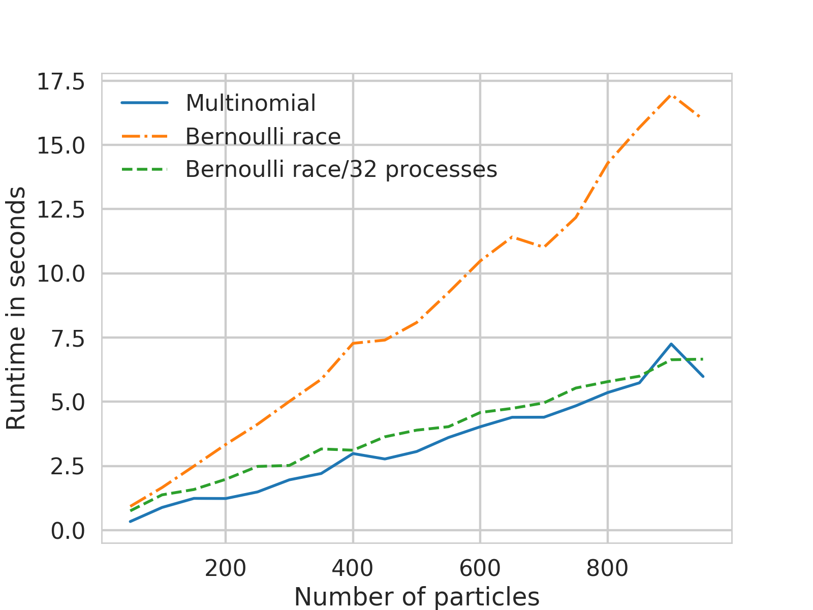
Figure 1 shows the run-time for RWPF and the BRPF for the Gaussian state space model. The BRPF clearly has linear complexity in the number of particles. In a sequential implementation the Bernoulli race (orange) performs worse than the classical resampling scheme (blue), but the difference vanishes when implementing a parallel version of the Bernoulli race (green, with 32 cores). This demonstrates the speedup due to parallel sampling of the coin flips. Since we need many Bernoulli random variables each of which is computationally cheap this algorithm lends itself to a implementation using GPUs to further improve the performance of the Bernoulli race.
Refer to caption
Figure 1: Comparison of the run-time for RWPF and BRPF for Gaussian state space model. For BRPF we show a sequential and a parallel implementation with 32 cores. For all algorithms we show wall-clock time for number of particles N𝑁N.

4.1.2 Efficiency

As alluded to earlier, if Bernoulli resampling is performed, the variance for any Monte Carlo estimate (4) will be the same as if the true weights were known and one applies standard multinomial resampling. From Proposition 1 it follows that the asymptotic variance of any Monte Carlo estimate of type (4) will be smaller when applying a BRPF over a RWPF. While the variance for functions (4) in the BRPF coincides with the standard particle filter we do not have access to the same estimator for the normalising constant and instead need to use the methods from Section 3.2.

For these reasons we will compare the performance of the BRPF with the RWPF for a set of different test functions h:𝖷T→ℝ:β„Žβ†’superscript𝖷𝑇ℝh\colon\mathsf{X}^{T}\rightarrow\mathbb{R} by comparing the variance of PF estimates (4). We then study the estimation of the normalizing constant separately. For the simulation we consider the functions

h1​(x1:T)subscriptβ„Ž1subscriptπ‘₯:1𝑇\displaystyle h_{1}(x_{1:T}) =1Tβ€‹βˆ‘t=1Txt,absent1𝑇superscriptsubscript𝑑1𝑇subscriptπ‘₯𝑑\displaystyle=\frac{1}{T}\sum_{t=1}^{T}x_{t}, h2​(x1:T)subscriptβ„Ž2subscriptπ‘₯:1𝑇\displaystyle\quad h_{2}(x_{1:T}) =β€–x1:Tβ€–2,absentsubscriptnormsubscriptπ‘₯:1𝑇2\displaystyle=\|x_{1:T}\|_{2},
h3​(x1:T)subscriptβ„Ž3subscriptπ‘₯:1𝑇\displaystyle h_{3}(x_{1:T}) =xT,absentsubscriptπ‘₯𝑇\displaystyle=x_{T}, h4​(x1:T)subscriptβ„Ž4subscriptπ‘₯:1𝑇\displaystyle\quad h_{4}(x_{1:T}) =(xTβˆ’xΒ―T)2,absentsuperscriptsubscriptπ‘₯𝑇subscriptΒ―π‘₯𝑇2\displaystyle=\left(x_{T}-\bar{x}_{T}\right)^{2},

where xΒ―T=βˆ‘i=1NxTi/NsubscriptΒ―π‘₯𝑇superscriptsubscript𝑖1𝑁superscriptsubscriptπ‘₯𝑇𝑖𝑁\bar{x}_{T}=\sum_{i=1}^{N}x_{T}^{i}/N. The PF approximations (4) using h3subscriptβ„Ž3h_{3} and h4subscriptβ„Ž4h_{4} are estimators for the quantities ΞΌT=∫xT​p​(d​xT∣y1:T)subscriptπœ‡π‘‡subscriptπ‘₯𝑇𝑝conditional𝑑subscriptπ‘₯𝑇subscript𝑦:1𝑇\mu_{T}=\int x_{T}p(dx_{T}\mid y_{1:T}) and ∫(xTβˆ’ΞΌT)2​p​(d​xT∣y1:T)superscriptsubscriptπ‘₯𝑇subscriptπœ‡π‘‡2𝑝conditional𝑑subscriptπ‘₯𝑇subscript𝑦:1𝑇\int\left(x_{T}-\mu_{T}\right)^{2}p(dx_{T}\mid y_{1:T}).

All estimates are based on 100 runs of each particle filter using N=100𝑁100N=100 particles. The results are collected in Table 1. We denote the standard deviation of the test functions under the BRPF as ΟƒBRPFsubscript𝜎BRPF\sigma_{\mathrm{BRPF}} and ΟƒRWPFsubscript𝜎RWPF\sigma_{\mathrm{RWPF}} for the RWPF. All measures indicate a reduction in the standard deviation. For the estimator of the function h1subscriptβ„Ž1h_{1}, the standard deviation is reduced by 26%percent2626\% when compared to the RWPF.

Table 1: For test functions hi,…​i=1,…,4formulae-sequencesubscriptβ„Žπ‘–β€¦π‘–1…4h_{i},\ldots i=1,\ldots,4 the standard deviation for RWPF and BRPF over 100 iterations.
Test function ΟƒRWPFsubscript𝜎RWPF\sigma_{\mathrm{RWPF}} ΟƒBRPFsubscript𝜎BRPF\sigma_{\mathrm{BRPF}} ΟƒBRPF/ΟƒRWPFsubscript𝜎BRPFsubscript𝜎RWPF\sigma_{\mathrm{BRPF}}/\sigma_{\mathrm{RWPF}}
h1subscriptβ„Ž1h_{1} 0.17 0.12 0.740.740.74
h2subscriptβ„Ž2h_{2} 0.93 0.78 0.840.840.84
h3subscriptβ„Ž3h_{3} 0.19 0.19 0.960.960.96
h4subscriptβ„Ž4h_{4} 0.42 0.40 0.940.940.94

We now investigate the estimates for the normalizing constant. TableΒ 2 shows the standard deviation of the (log-)normalizing constant of a Gaussian state space model for T=50𝑇50T=50 time steps. In this setting it is not obvious why the Bernoulli race resampling estimate should outperform the estimate provided by the RWPF. In our case however, we find that the BRPF performs better.

Table 2: Comparison of the normalizing constant estimate for different implementations of the particle filter.
sd​(log⁑p^​(y1:T))sd^𝑝subscript𝑦:1𝑇\mathrm{sd}(\log\hat{p}(y_{1:T}))
BRPF 0.55
RWPF 0.66

4.2 Partially Observed Diffusion

We use the sine diffusion, a commonly used example in the context of partially observed diffusions, see e.g. [fearnhead2008particle], given by the stochastic differential equation (SDE)

d​Xs=sin⁑(Xs)​d​t+d​Bs,s∈[0,15].formulae-sequence𝑑subscript𝑋𝑠subscript𝑋𝑠𝑑𝑑𝑑subscript𝐡𝑠𝑠015dX_{s}=\sin(X_{s})dt+dB_{s},\quad s\in[0,15].

Here, (Bs)s∈[0,15]subscriptsubscript𝐡𝑠𝑠015(B_{s})_{s\in[0,15]} denotes a Brownian motion and the drift function in (6) is a​(x)=sin⁑(x).π‘Žπ‘₯π‘₯a(x)=\sin(x). Consequently, A​(x)=βˆ’cos⁑(x)𝐴π‘₯π‘₯A(x)=-\cos(x) and with Ο•(x)=(sin(x)2+cos(x))/2\phi(x)=\left(\sin(x)^{2}+\cos(x)\right)/2, the transition density is

fΔ​t​(x,y)subscript𝑓Δ𝑑π‘₯𝑦\displaystyle f_{\Delta t}(x,y) =φ​(y;x,Δ​t)​exp⁑(βˆ’cos⁑(y)+cos⁑(x))absentπœ‘π‘¦π‘₯Δ𝑑𝑦π‘₯\displaystyle=\varphi(y;x,\Delta t)\exp\left(-\cos(y)+\cos(x)\right)
×𝔼​[exp⁑(βˆ’βˆ«0Δ​tϕ​(Ws)​𝑑s)].absent𝔼delimited-[]superscriptsubscript0Δ𝑑italic-Ο•subscriptπ‘Šπ‘ differential-d𝑠\displaystyle\quad\times\mathbb{E}\left[\exp\left(-\int_{0}^{\Delta t}\phi(W_{s})ds\right)\right]. (18)

We observe the state of the SDE through zero mean Gaussian noise with standard deviation 5 yielding weights

w​(xtβˆ’1,xt,yt)=φ​(yt;xt,52)​fΔ​t​(xt∣xtβˆ’1)q​(xt∣xtβˆ’1,yt),𝑀subscriptπ‘₯𝑑1subscriptπ‘₯𝑑subscriptπ‘¦π‘‘πœ‘subscript𝑦𝑑subscriptπ‘₯𝑑superscript52subscript𝑓Δ𝑑conditionalsubscriptπ‘₯𝑑subscriptπ‘₯𝑑1π‘žconditionalsubscriptπ‘₯𝑑subscriptπ‘₯𝑑1subscript𝑦𝑑w(x_{t-1},x_{t},y_{t})=\frac{\varphi(y_{t};x_{t},5^{2})f_{\Delta t}(x_{t}\mid x_{t-1})}{q(x_{t}\mid x_{t-1},y_{t})},

As the proposal q(β‹…βˆ£xtβˆ’1,yt)q(\cdot\mid x_{t-1},y_{t}) we take one step of the Euler–Maruyama scheme.
Refer to caption
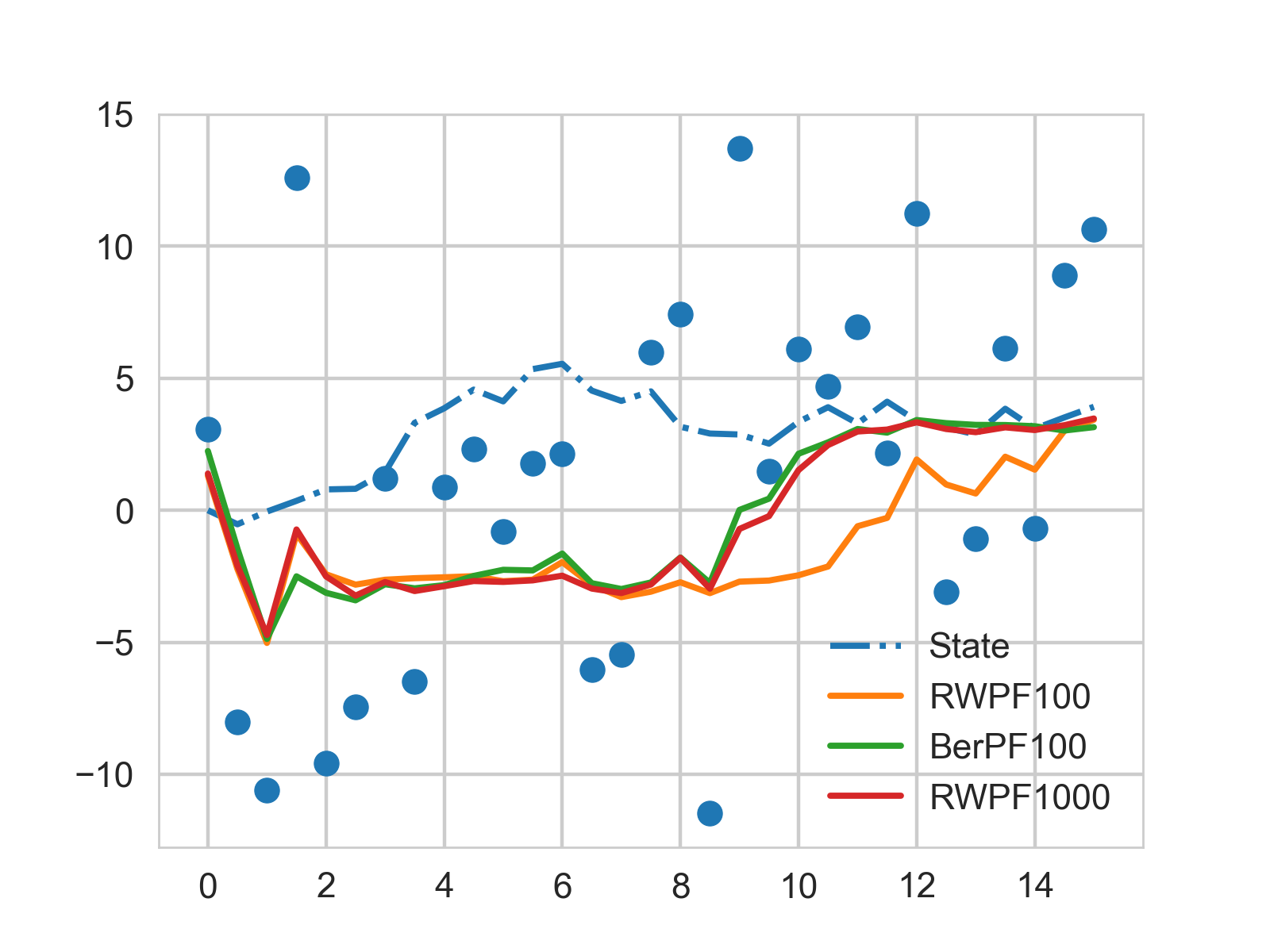
Figure 2: Tracking performance for different particle filters; RWPF with 100 particles (RWPF100) and 1000 particles (RWPF1000) as well as a particle filter using Bernoulli resampling with 100 particles (BerPF100).

The weights are intractable because of the expectation on the right-hand side in (18). The construction of unbiased coin flips can often rely on similar techniques as the construction of unbiased estimators. We can construct an unbiased estimator for the transition density in the following way. Fix a Brownian bridge (Ws)s∈[0,Δ​t]subscriptsubscriptπ‘Šπ‘ π‘ 0Δ𝑑\left(W_{s}\right)_{s\in[0,\Delta t]} starting at xπ‘₯x and finishing at y𝑦y. Sample κ∼Pois​(λ​Δ​t)similar-toπœ…Poisπœ†Ξ”π‘‘\kappa\sim\mathrm{Pois}(\lambda\Delta t), U1​…,Uκ∼U​[0,Δ​t]similar-tosubscriptπ‘ˆ1…subscriptπ‘ˆπœ…π‘ˆ0Δ𝑑U_{1}\ldots,U_{\kappa}\sim U[0,\Delta t] then the Poisson estimator [Beskos2006] is given by

P^​(ΞΊ,U1​…,UΞΊ)=exp⁑{(Ξ»βˆ’c)​Δ​t}β€‹βˆi=1ΞΊ{cβˆ’Ο•β€‹(WUi)}Ξ»,^π‘ƒπœ…subscriptπ‘ˆ1…subscriptπ‘ˆπœ…πœ†π‘Ξ”π‘‘superscriptsubscriptproduct𝑖1πœ…π‘italic-Ο•subscriptπ‘Šsubscriptπ‘ˆπ‘–πœ†\hat{P}(\kappa,U_{1}\ldots,U_{\kappa})=\exp\left\{\left(\lambda-c\right)\Delta t\right\}\prod_{i=1}^{\kappa}\frac{\left\{c-\phi\left(W_{U_{i}}\right)\right\}}{\lambda},

where c𝑐c is chosen such that the estimator is non-negative. The Poisson estimator is unbiased

𝔼​[P^​(ΞΊ,U1​…,UΞΊ)]=𝔼​[exp⁑(βˆ’βˆ«0Δ​tϕ​(Ws)​𝑑s)].𝔼delimited-[]^π‘ƒπœ…subscriptπ‘ˆ1…subscriptπ‘ˆπœ…π”Όdelimited-[]superscriptsubscript0Δ𝑑italic-Ο•subscriptπ‘Šπ‘ differential-d𝑠\mathbb{E}\left[\hat{P}(\kappa,U_{1}\ldots,U_{\kappa})\right]=\mathbb{E}\left[\exp\left(-\int_{0}^{\Delta t}\phi(W_{s})ds\right)\right]. (19)
Refer to caption
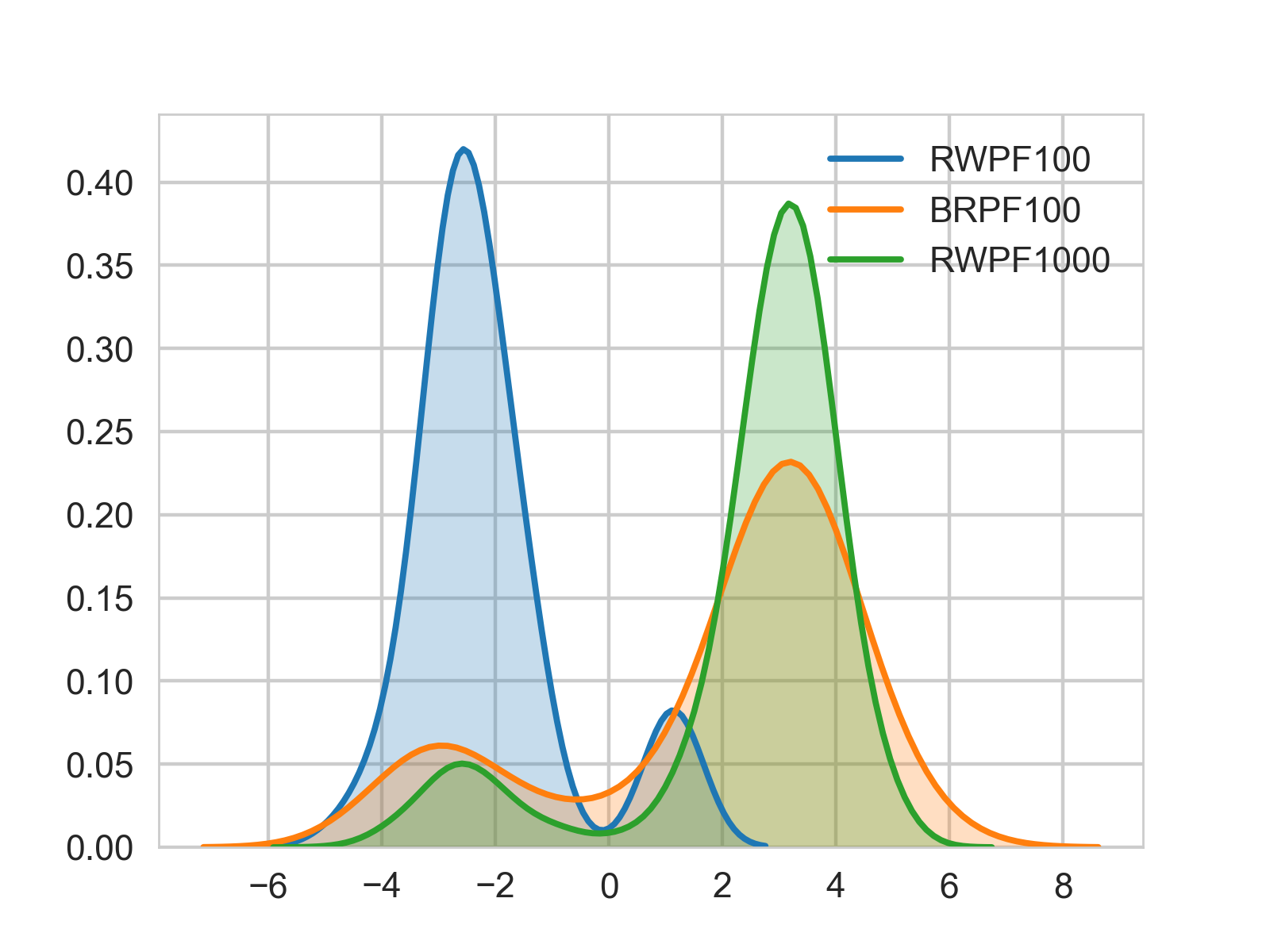
Figure 3: Kernel density estimate of p​(x10∣y1:10)𝑝conditionalsubscriptπ‘₯10subscript𝑦:110p(x_{10}\mid y_{1:10}) based on particle approximations from a RWPF with 100 particles (RWPF) a BRPF with 100 particles (Bernoulli) and a RWPF with 1000 particles.

For the purposes of implementing the BRPF, we need to construct a coin flip with success probability proportional to (19). We use the probability generating function approach which works analogously to the Poisson estimator. Sample κ∼Pois​(λ​Δ​t),Vi∼Unif​[0,1],i=1,…​κformulae-sequencesimilar-toπœ…Poisπœ†Ξ”π‘‘formulae-sequencesimilar-tosubscript𝑉𝑖Unif01𝑖1β€¦πœ…\kappa\sim\mathrm{Pois}(\lambda\Delta t),V_{i}\sim\mathrm{Unif}[0,1],i=1,\ldots\kappa, then

Z=∏i=1ΞΊ1​{Vi≀{cβˆ’Ο•β€‹(WUi)}Ξ»}𝑍superscriptsubscriptproduct𝑖1πœ…1subscript𝑉𝑖𝑐italic-Ο•subscriptπ‘Šsubscriptπ‘ˆπ‘–πœ†Z=\prod_{i=1}^{\kappa}1\left\{V_{i}\leq\frac{\left\{c-\phi\left(W_{U_{i}}\right)\right\}}{\lambda}\right\}

has success probability

exp⁑{(cβˆ’Ξ»)​Δ​t}​𝔼​[exp⁑(βˆ’βˆ«0Δ​tϕ​(Ws)​𝑑s)].π‘πœ†Ξ”π‘‘π”Όdelimited-[]superscriptsubscript0Δ𝑑italic-Ο•subscriptπ‘Šπ‘ differential-d𝑠\exp\left\{(c-\lambda)\Delta t\right\}\mathbb{E}\left[\exp\left(-\int_{0}^{\Delta t}\phi(W_{s})ds\right)\right].

Hence, to implement the BRPF we can choose

ct,ksubscriptπ‘π‘‘π‘˜\displaystyle c_{t,k} =φ​(yt;xt,52)​φ​(xt;xtβˆ’1,Δ​t)φ​(yt;xtβˆ’1+Δ​t​sin⁑(xtβˆ’1),Δ​t)absentπœ‘subscript𝑦𝑑subscriptπ‘₯𝑑superscript52πœ‘subscriptπ‘₯𝑑subscriptπ‘₯𝑑1Ξ”π‘‘πœ‘subscript𝑦𝑑subscriptπ‘₯𝑑1Δ𝑑subscriptπ‘₯𝑑1Δ𝑑\displaystyle=\frac{\varphi(y_{t};x_{t},5^{2})\varphi(x_{t};x_{t-1},\Delta t)}{\varphi(y_{t};x_{t-1}+\Delta t\sin(x_{t-1}),\Delta t)}
Γ—exp⁑(βˆ’cos⁑(xt)+cos⁑(xtβˆ’1)βˆ’(cβˆ’Ξ»)​Δ​t)absentsubscriptπ‘₯𝑑subscriptπ‘₯𝑑1π‘πœ†Ξ”π‘‘\displaystyle\quad\times\exp\left(-\cos(x_{t})+\cos(x_{t-1})-(c-\lambda)\Delta t\right)
bt,ksubscriptπ‘π‘‘π‘˜\displaystyle b_{t,k} =exp⁑{(cβˆ’Ξ»)​Δ​t}​𝔼​[exp⁑(βˆ’βˆ«0Δ​tϕ​(Wsk)​𝑑s)],absentπ‘πœ†Ξ”π‘‘π”Όdelimited-[]superscriptsubscript0Δ𝑑italic-Ο•superscriptsubscriptπ‘Šπ‘ π‘˜differential-d𝑠\displaystyle=\exp\left\{(c-\lambda)\Delta t\right\}\mathbb{E}\left[\exp\left(-\int_{0}^{\Delta t}\phi(W_{s}^{k})ds\right)\right],

where (Wsk)s∈[0,Δ​t]subscriptsuperscriptsubscriptπ‘Šπ‘ π‘˜π‘ 0Δ𝑑(W_{s}^{k})_{s\in[0,\Delta t]} denotes a Brownian bridge from xtβˆ’1ksuperscriptsubscriptπ‘₯𝑑1π‘˜x_{t-1}^{k} to xtksuperscriptsubscriptπ‘₯π‘‘π‘˜x_{t}^{k}.

4.2.1 Complexity and Run-time

As in the previous example, we observe the BRPF to be of order O​(N)𝑂𝑁O(N) and slower than the RWPF. However, implementing the Bernoulli race in parallel yields almost the same performance in terms of run-time. The details can be found in the supplementary material.

4.2.2 Efficiency

One run for the RWPF and the BRPF is shown in FigureΒ 2, where we show the true state of the SDE as well as the noisy observations and the particle filter approximations. In this scenario precise state estimation is hampered by the high noise and resulting partial multimodality of the filtering distribution as shown in FigureΒ 3. For N=100𝑁100N=100, FigureΒ 2 shows that the BRPF performs much better as it finds the true state earlier. The RWPF finds this trajectory only when the number of particles is increased (here we show also the case N=1000𝑁1000N=1000). With the same test functions as above we compare both algorithms in TableΒ 3. We observe gains for all functions, with the most significant gain for the conditional mean, h3subscriptβ„Ž3h_{3}. Again, the Bernoulli race will ordinarily be slower, but most of the difference in run-time vanishes when the Bernoulli race is implemented in parallel. Further details are provided in the supplementary material.

Table 3: Comparison of the normalizing constant estimate for different implementations of the particle filter.
Test function ΟƒRWBFsubscript𝜎RWBF\sigma_{\mathrm{RWBF}} ΟƒBRPFsubscript𝜎BRPF\sigma_{\mathrm{BRPF}} ΟƒBRPF/ΟƒRWPFsubscript𝜎BRPFsubscript𝜎RWPF\sigma_{\mathrm{BRPF}}/\sigma_{\mathrm{RWPF}}
h1subscriptβ„Ž1h_{1} 1.41 1.27 0.91
h2subscriptβ„Ž2h_{2} 1.61 1.58 0.98
h3subscriptβ„Ž3h_{3} 1.26 0.64 0.50
h4subscriptβ„Ž4h_{4} 1.09 0.87 0.80
Table 4: Comparison of the normalizing constant estimate for different implementations of the particle filter.
sd​(log⁑p^​(y1:T))sd^𝑝subscript𝑦:1𝑇\mathrm{sd}(\log\hat{p}(y_{1:T}))
RWPF 3.83
BRPF 3.11
Bootstrap 3.13

As a final test we use both particle filters for estimating the (log\log-)normalizing constant. The results are listed in TableΒ 4. For comparison we also employ a bootstrap particle filter using the exact algorithm [beskos2005exact] to propose from the model. We observed this implementation to be slower than the other two. The BRPF estimate (17) outperforms the RWPF and the bootstrap PF.

5 Conclusion

We have introduced the idea of Bernoulli races to resampling in particle filtering, utilizing the equivalence of unbiased estimation and the construction of unbiased coin-flips. This algorithm provides the first resampling scheme to allow for exact implementation of multinomial resampling when the weights are intractable, but unbiased estimates are available. We have shown that our algorithm has a complexity of order N𝑁N, like standard multinomial resampling, and demonstrated its advantages over alternative methods in a variety of settings. In doing so we have focused our attention to the resampling step. Further gains using our algorithm could be obtained by considering auxiliary particle filters and to resample only if the effective sample size drops beyond a certain threshold. We expect both to positively impact the performance of the BRPF.

Β 

Supplementary Material to Bernoulli Race Particle Filters


Β 

Appendix A Proofs

When we say that T𝑇T is a geometric random variable with parameter, or success probability, p𝑝p we mean that

ℙ​(Tβ‰₯k)=(1βˆ’p)k,kβ‰₯1.formulae-sequenceβ„™π‘‡π‘˜superscript1π‘π‘˜π‘˜1\mathbb{P}(T\geq k)=(1-p)^{k},\qquad k\geq 1.
Proposition 3.

Assume limNβ†’βˆžΟN=:ρ∈(0,1)\lim_{N\rightarrow\infty}\rho_{N}=:\rho\in(0,1). Then we have the following central limit theorem for the average number of coin flips as Nβ†’βˆžβ†’π‘N\rightarrow\infty

N​(1Nβ€‹βˆ‘j=1NCj,Nβˆ’1ρN)​→𝑑​𝒩​(0,1βˆ’ΟΟ2),𝑁1𝑁superscriptsubscript𝑗1𝑁subscript𝐢𝑗𝑁1subscriptπœŒπ‘π‘‘β†’π’©01𝜌superscript𝜌2\sqrt{N}\left(\frac{1}{N}\sum_{j=1}^{N}C_{j,N}-\frac{1}{\rho_{N}}\right)\overset{d}{\rightarrow}\mathcal{N}\left(0,\frac{1-\rho}{\rho^{2}}\right),

where →𝑑𝑑→\overset{d}{\rightarrow} denotes convergence in distribution.

Proof.

The random variables Zi,N=(Ci,Nβˆ’1/ρN)/Nsubscript𝑍𝑖𝑁subscript𝐢𝑖𝑁1subscriptπœŒπ‘π‘Z_{i,N}=\left(C_{i,N}-1/\rho_{N}\right)/\sqrt{N} form a triangular array

{Zi,N;i=1,…​N,Nβˆˆβ„•}formulae-sequencesubscript𝑍𝑖𝑁𝑖1…𝑁𝑁ℕ\left\{Z_{i,N};i=1,\ldots N,N\in\mathbb{N}\right\}

of row wise independent random variables. Define sN2=βˆ‘i=1Nvar​(Zi,N)=(1βˆ’ΟN)/ρN2superscriptsubscript𝑠𝑁2superscriptsubscript𝑖1𝑁varsubscript𝑍𝑖𝑁1subscriptπœŒπ‘superscriptsubscriptπœŒπ‘2s_{N}^{2}=\sum_{i=1}^{N}\mathrm{var}\left(Z_{i,N}\right)=\left(1-\rho_{N}\right)/\rho_{N}^{2} and notice that sN2β†’1βˆ’Οβˆˆ(0,1)β†’superscriptsubscript𝑠𝑁21𝜌01s_{N}^{2}\to 1-\rho\in(0,1) as Nβ†’βˆžβ†’π‘N\to\infty. In addition one can easily show that 𝔼​[|Z1,N|3]𝔼delimited-[]superscriptsubscript𝑍1𝑁3\mathbb{E}[|Z_{1,N}|^{3}] are bounded uniformly in N𝑁N and therefore

1sN3β€‹βˆ‘i=1N𝔼​[Zi,N]1superscriptsubscript𝑠𝑁3superscriptsubscript𝑖1𝑁𝔼delimited-[]subscript𝑍𝑖𝑁\displaystyle\frac{1}{s_{N}^{3}}\sum_{i=1}^{N}\mathbb{E}\left[Z_{i,N}\right] =ρN3/2(1βˆ’ΟN)3​NN3/2​𝔼​[|Z1,N|3]absentsuperscriptsubscriptπœŒπ‘32superscript1subscriptπœŒπ‘3𝑁superscript𝑁32𝔼delimited-[]superscriptsubscript𝑍1𝑁3\displaystyle=\frac{\rho_{N}^{3/2}}{(1-\rho_{N})^{3}}\frac{N}{N^{3/2}}\mathbb{E}\left[\left|Z_{1,N}\right|^{3}\right]
≀CNβ†’0,asΒ Nβ†’βˆž,formulae-sequenceabsent𝐢𝑁→0asΒ Nβ†’βˆž\displaystyle\leq\frac{C}{\sqrt{N}}\to 0,\qquad\text{as $N\to\infty$},

that is the Lyapunov condition is satisfied and therefore Nβ†’βˆžβ†’π‘N\rightarrow\infty

1Nβ€‹βˆ‘i=1N(Ci,Nβˆ’1ρN)​→𝑑​𝒩​(0,s2),1𝑁superscriptsubscript𝑖1𝑁subscript𝐢𝑖𝑁1subscriptπœŒπ‘π‘‘β†’π’©0superscript𝑠2\frac{1}{\sqrt{N}}\sum_{i=1}^{N}\left(C_{i,N}-\frac{1}{\rho_{N}}\right)\overset{d}{\rightarrow}\mathcal{N}\left(0,s^{2}\right),

where s2=limNβ†’βˆžsN2=(1βˆ’Ο)/ρ2.superscript𝑠2subscript→𝑁superscriptsubscript𝑠𝑁21𝜌superscript𝜌2s^{2}=\lim_{N\rightarrow\infty}s_{N}^{2}=(1-\rho)/\rho^{2}. ∎

Proposition 4.

For Nβˆˆβ„•π‘β„•N\in\mathbb{N} let C1,N,…,CN,Nsubscript𝐢1𝑁…subscript𝐢𝑁𝑁C_{1,N},\ldots,C_{N,N} denote independent samples from a geometric distribution with success probability ρNsubscriptπœŒπ‘\rho_{N}, then the minimum variance unbiased estimator for ρNsubscriptπœŒπ‘\rho_{N} is

ρ^Nmvue=Nβˆ’1βˆ‘k=1NCk,Nβˆ’1.superscriptsubscript^πœŒπ‘mvue𝑁1superscriptsubscriptπ‘˜1𝑁subscriptπΆπ‘˜π‘1\hat{\rho}_{N}^{\mathrm{mvue}}=\frac{N-1}{\sum_{k=1}^{N}C_{k,N}-1}. (20)
Proof.

This is a straightforward application of the Lehmann-ScheffΓ© Theorem [hogg2005introduction, Theorem 7.4.1]. Take the unbiased estimator 1​{C1,N=1}1subscript𝐢1𝑁11\left\{C_{1,N}=1\right\}, where 1​{A}1𝐴1\{A\} denotes the indicator function of the set A𝐴A, and condition on the complete and sufficient statistic (of the coin flips) βˆ‘k=1NCk,Nsuperscriptsubscriptπ‘˜1𝑁subscriptπΆπ‘˜π‘\sum_{k=1}^{N}C_{k,N}. A straightforward calculation yields

𝔼​[1​{C1,N=1}βˆ£βˆ‘k=1NCk,N=n]𝔼delimited-[]conditional1subscript𝐢1𝑁1superscriptsubscriptπ‘˜1𝑁subscriptπΆπ‘˜π‘π‘›\displaystyle\mathbb{E}\left[1\left\{C_{1,N}=1\right\}\mid\sum_{k=1}^{N}C_{k,N}=n\right] =ℙ​(C1=1,βˆ‘k=2NCk,N=nβˆ’1)ℙ​(βˆ‘k=1NCk,N=n)absentβ„™formulae-sequencesubscript𝐢11superscriptsubscriptπ‘˜2𝑁subscriptπΆπ‘˜π‘π‘›1β„™superscriptsubscriptπ‘˜1𝑁subscriptπΆπ‘˜π‘π‘›\displaystyle=\frac{\mathbb{P}\left(C_{1}=1,\sum_{k=2}^{N}C_{k,N}=n-1\right)}{\mathbb{P}\left(\sum_{k=1}^{N}C_{k,N}=n\right)}
=p​(nβˆ’2Nβˆ’2)​pNβˆ’1​(1βˆ’p)nβˆ’N(nβˆ’1Nβˆ’1)​pN​(1βˆ’p)nβˆ’Nabsent𝑝binomial𝑛2𝑁2superscript𝑝𝑁1superscript1𝑝𝑛𝑁binomial𝑛1𝑁1superscript𝑝𝑁superscript1𝑝𝑛𝑁\displaystyle=\frac{p\binom{n-2}{N-2}p^{N-1}(1-p)^{n-N}}{\binom{n-1}{N-1}p^{N}(1-p)^{n-N}}
=Nβˆ’1nβˆ’1absent𝑁1𝑛1\displaystyle=\frac{N-1}{n-1}

and thus

ρ^Nmvue=𝔼​[1​{C1,N=1}βˆ£βˆ‘k=1NCk,N]=Nβˆ’1βˆ‘k=1NCk,Nβˆ’1.∎superscriptsubscript^πœŒπ‘mvue𝔼delimited-[]conditional1subscript𝐢1𝑁1superscriptsubscriptπ‘˜1𝑁subscriptπΆπ‘˜π‘π‘1superscriptsubscriptπ‘˜1𝑁subscriptπΆπ‘˜π‘1\hat{\rho}_{N}^{\mathrm{mvue}}=\mathbb{E}\left[1\left\{C_{1,N}=1\right\}\mid\sum_{k=1}^{N}C_{k,N}\right]=\frac{N-1}{\sum_{k=1}^{N}C_{k,N}-1}.\qed
Proposition 5.

For Nβˆˆβ„•π‘β„•N\in\mathbb{N} let C1,N,C2,N,…subscript𝐢1𝑁subscript𝐢2𝑁…C_{1,N},C_{2,N},\ldots denote independent samples from a Geometric distribution with success probability ρNsubscriptπœŒπ‘\rho_{N}, then

N​(ρ^Nmvueβˆ’ΟN)​→𝑑​𝒩​(0,(1βˆ’Ο)​ρ2).𝑁superscriptsubscript^πœŒπ‘mvuesubscriptπœŒπ‘π‘‘β†’π’©01𝜌superscript𝜌2\sqrt{N}\left(\hat{\rho}_{N}^{\mathrm{mvue}}-\rho_{N}\right)\overset{d}{\rightarrow}\mathcal{N}\left(0,\left(1-\rho\right)\rho^{2}\right).
Proof.

By Proposition 3 we have convergence

N​(1Nβ€‹βˆ‘i=1NCi,Nβˆ’1ρN)​→𝑑​𝒩​(0,1βˆ’ΟΟ2).𝑁1𝑁superscriptsubscript𝑖1𝑁subscript𝐢𝑖𝑁1subscriptπœŒπ‘π‘‘β†’π’©01𝜌superscript𝜌2\sqrt{N}\left(\frac{1}{N}\sum_{i=1}^{N}C_{i,N}-\frac{1}{\rho_{N}}\right)\overset{d}{\rightarrow}\mathcal{N}\left(0,\frac{1-\rho}{\rho^{2}}\right).

In addition,

|N​(βˆ‘i=1NCi,Nβˆ’1Nβˆ’1βˆ’1ρN)βˆ’N​(1Nβ€‹βˆ‘i=1NCi,Nβˆ’1ρN)|𝑁superscriptsubscript𝑖1𝑁subscript𝐢𝑖𝑁1𝑁11subscriptπœŒπ‘π‘1𝑁superscriptsubscript𝑖1𝑁subscript𝐢𝑖𝑁1subscriptπœŒπ‘\displaystyle\left|\sqrt{N}\left(\frac{\sum_{i=1}^{N}C_{i,N}-1}{N-1}-\frac{1}{\rho_{N}}\right)-\sqrt{N}\left(\frac{1}{N}\sum_{i=1}^{N}C_{i,N}-\frac{1}{\rho_{N}}\right)\right| β†’0β†’absent0\displaystyle\rightarrow 0

almost surely, so

N​(βˆ‘i=1NCi,Nβˆ’1Nβˆ’1βˆ’1ρN)​→𝑑​𝒩​(0,1βˆ’ΟΟ2).𝑁superscriptsubscript𝑖1𝑁subscript𝐢𝑖𝑁1𝑁11subscriptπœŒπ‘π‘‘β†’π’©01𝜌superscript𝜌2\sqrt{N}\left(\frac{\sum_{i=1}^{N}C_{i,N}-1}{N-1}-\frac{1}{\rho_{N}}\right)\overset{d}{\rightarrow}\mathcal{N}\left(0,\frac{1-\rho}{\rho^{2}}\right).

By the δ𝛿\delta-Method with g​(x)=1/x𝑔π‘₯1π‘₯g(x)=1/x, |g′​(x)|=1/x2superscript𝑔′π‘₯1superscriptπ‘₯2|g^{\prime}(x)|=1/x^{2} we obtain

N​(g​(βˆ‘i=1NCi,Nβˆ’1Nβˆ’1)βˆ’g​(1ρN))𝑁𝑔superscriptsubscript𝑖1𝑁subscript𝐢𝑖𝑁1𝑁1𝑔1subscriptπœŒπ‘\displaystyle\sqrt{N}\left(g\left(\frac{\sum_{i=1}^{N}C_{i,N}-1}{N-1}\right)-g\left(\frac{1}{\rho_{N}}\right)\right) =N​(Nβˆ’1βˆ‘Ci,Nβˆ’1βˆ’ΟN)absent𝑁𝑁1subscript𝐢𝑖𝑁1subscriptπœŒπ‘\displaystyle=\sqrt{N}\left(\frac{N-1}{\sum C_{i,N}-1}-\rho_{N}\right)
→𝑑​𝒩​(0,1βˆ’ΟΟ2⋅ρ4)=𝒩​(0,(1βˆ’Ο)​ρ2).βˆŽπ‘‘β†’π’©0β‹…1𝜌superscript𝜌2superscript𝜌4𝒩01𝜌superscript𝜌2\displaystyle\overset{d}{\rightarrow}\mathcal{N}\left(0,\frac{1-\rho}{\rho^{2}}\cdot\rho^{4}\right)=\mathcal{N}\left(0,\left(1-\rho\right)\rho^{2}\right).\qed
Theorem 6.

The estimator

ρ^N,T=∏t=1T1Nβ€‹βˆ‘k=1Nctkβ‹…Nβˆ’1βˆ‘k=1NCk,Nβˆ’1.subscript^πœŒπ‘π‘‡superscriptsubscriptproduct𝑑1𝑇1𝑁superscriptsubscriptπ‘˜1𝑁⋅superscriptsubscriptπ‘π‘‘π‘˜π‘1superscriptsubscriptπ‘˜1𝑁subscriptπΆπ‘˜π‘1\hat{\rho}_{N,T}=\prod_{t=1}^{T}\frac{1}{N}\sum_{k=1}^{N}c_{t}^{k}\cdot\frac{N-1}{\sum_{k=1}^{N}C_{k,N}-1}.

is unbiased for p​(y1:T)𝑝subscript𝑦:1𝑇p(y_{1:T}), i.e.

𝔼​[ρ^N,T]=p​(y1:T).𝔼delimited-[]subscript^πœŒπ‘π‘‡π‘subscript𝑦:1𝑇\mathbb{E}\left[\hat{\rho}_{N,T}\right]=p(y_{1:T}).
Proof.

The main argument is that the standard proof for unbiasedness using backward induction can be adapted to include our estimator using the geometric random variables C1,N,…,CN,Nsubscript𝐢1𝑁…subscript𝐢𝑁𝑁C_{1,N},\ldots,C_{N,N}. Denote by X,X¯𝑋¯𝑋X,\overline{X} the random variables before and after resampling respectively. Then we have

𝔼​[1Nβ€‹βˆ‘i=1NwTk∣XTβˆ’11:N]𝔼delimited-[]conditional1𝑁superscriptsubscript𝑖1𝑁superscriptsubscriptπ‘€π‘‡π‘˜superscriptsubscript𝑋𝑇1:1𝑁\displaystyle\mathbb{E}\left[\frac{1}{N}\sum_{i=1}^{N}w_{T}^{k}\mid{X}_{T-1}^{1:N}\right]
=𝔼​[1Nβ€‹βˆ‘i=1Ng​(yT∣XTi)∣XTβˆ’11:N]absent𝔼delimited-[]conditional1𝑁superscriptsubscript𝑖1𝑁𝑔conditionalsubscript𝑦𝑇superscriptsubscript𝑋𝑇𝑖superscriptsubscript𝑋𝑇1:1𝑁\displaystyle=\mathbb{E}\left[\frac{1}{N}\sum_{i=1}^{N}g(y_{T}\mid{X}_{T}^{i})\mid{X}_{T-1}^{1:N}\right]
=1Nβ€‹βˆ‘i=1N∫g​(yT∣xTi)​p​(xTi∣XTβˆ’11:N)​𝑑xTiabsent1𝑁superscriptsubscript𝑖1𝑁𝑔conditionalsubscript𝑦𝑇superscriptsubscriptπ‘₯𝑇𝑖𝑝conditionalsuperscriptsubscriptπ‘₯𝑇𝑖superscriptsubscript𝑋𝑇1:1𝑁differential-dsuperscriptsubscriptπ‘₯𝑇𝑖\displaystyle=\frac{1}{N}\sum_{i=1}^{N}\int g(y_{T}\mid{x}_{T}^{i})p(x_{T}^{i}\mid{X}_{T-1}^{1:N})dx_{T}^{i}
=1Nβ€‹βˆ‘i=1N∫g​(yT∣xTi)β€‹βˆ‘j=1Nf​(xTi∣XTβˆ’1j)​g​(yTβˆ’1∣XTβˆ’1j)βˆ‘k=1Ng​(yTβˆ’1∣XTβˆ’1k)​d​xTiabsent1𝑁superscriptsubscript𝑖1𝑁𝑔conditionalsubscript𝑦𝑇superscriptsubscriptπ‘₯𝑇𝑖superscriptsubscript𝑗1𝑁𝑓conditionalsuperscriptsubscriptπ‘₯𝑇𝑖superscriptsubscript𝑋𝑇1𝑗𝑔conditionalsubscript𝑦𝑇1superscriptsubscript𝑋𝑇1𝑗superscriptsubscriptπ‘˜1𝑁𝑔conditionalsubscript𝑦𝑇1superscriptsubscript𝑋𝑇1π‘˜π‘‘superscriptsubscriptπ‘₯𝑇𝑖\displaystyle=\frac{1}{N}\sum_{i=1}^{N}\int g(y_{T}\mid x_{T}^{i})\sum_{j=1}^{N}f(x_{T}^{i}\mid{X}_{T-1}^{j})\frac{g(y_{T-1}\mid{X}_{T-1}^{j})}{\sum_{k=1}^{N}g(y_{T-1}\mid{X}_{T-1}^{k})}d{x}_{T}^{i}
=1Nβ€‹βˆ‘i=1Nβˆ‘j=1N∫g​(yT∣xTi)​f​(xTi∣XTβˆ’1j)​g​(yTβˆ’1∣XTβˆ’1j)βˆ‘k=1Ng​(yTβˆ’1∣XTβˆ’1k)​𝑑xTiabsent1𝑁superscriptsubscript𝑖1𝑁superscriptsubscript𝑗1𝑁𝑔conditionalsubscript𝑦𝑇superscriptsubscriptπ‘₯𝑇𝑖𝑓conditionalsuperscriptsubscriptπ‘₯𝑇𝑖superscriptsubscript𝑋𝑇1𝑗𝑔conditionalsubscript𝑦𝑇1superscriptsubscript𝑋𝑇1𝑗superscriptsubscriptπ‘˜1𝑁𝑔conditionalsubscript𝑦𝑇1superscriptsubscript𝑋𝑇1π‘˜differential-dsuperscriptsubscriptπ‘₯𝑇𝑖\displaystyle=\frac{1}{N}\sum_{i=1}^{N}\sum_{j=1}^{N}\int g(y_{T}\mid x_{T}^{i})f(x_{T}^{i}\mid{X}_{T-1}^{j})\frac{g(y_{T-1}\mid{X}_{T-1}^{j})}{\sum_{k=1}^{N}g(y_{T-1}\mid{X}_{T-1}^{k})}d{x}_{T}^{i}
=1Nβ€‹βˆ‘i=1Nβˆ‘j=1Np​(yT∣XTβˆ’1j)​g​(yTβˆ’1∣XTβˆ’1j)βˆ‘k=1Ng​(yTβˆ’1∣XTβˆ’1k)absent1𝑁superscriptsubscript𝑖1𝑁superscriptsubscript𝑗1𝑁𝑝conditionalsubscript𝑦𝑇superscriptsubscript𝑋𝑇1𝑗𝑔conditionalsubscript𝑦𝑇1superscriptsubscript𝑋𝑇1𝑗superscriptsubscriptπ‘˜1𝑁𝑔conditionalsubscript𝑦𝑇1superscriptsubscript𝑋𝑇1π‘˜\displaystyle=\frac{1}{N}\sum_{i=1}^{N}\sum_{j=1}^{N}p(y_{T}\mid X_{T-1}^{j})\frac{g(y_{T-1}\mid{X}_{T-1}^{j})}{\sum_{k=1}^{N}g(y_{T-1}\mid{X}_{T-1}^{k})}
=βˆ‘j=1Np​(yTβˆ’1:T∣XTβˆ’1j)βˆ‘k=1Ng​(yTβˆ’1∣XTβˆ’1k).absentsuperscriptsubscript𝑗1𝑁𝑝conditionalsubscript𝑦:𝑇1𝑇superscriptsubscript𝑋𝑇1𝑗superscriptsubscriptπ‘˜1𝑁𝑔conditionalsubscript𝑦𝑇1superscriptsubscript𝑋𝑇1π‘˜\displaystyle=\frac{\sum_{j=1}^{N}p(y_{T-1:T}\mid{X}_{T-1}^{j})}{\sum_{k=1}^{N}g(y_{T-1}\mid{X}_{T-1}^{k})}.

Now, considering the case where we estimate the weights using the geometric random variables, we have

𝔼​[1Nβ€‹βˆ‘k=1NcTkβ‹…Nβˆ’1βˆ‘k=1NCk,N,Tβˆ’1∣XTβˆ’11:N]𝔼delimited-[]conditional1𝑁superscriptsubscriptπ‘˜1𝑁⋅superscriptsubscriptπ‘π‘‡π‘˜π‘1superscriptsubscriptπ‘˜1𝑁subscriptπΆπ‘˜π‘π‘‡1superscriptsubscript𝑋𝑇1:1𝑁\displaystyle\mathbb{E}\left[\frac{1}{N}\sum_{k=1}^{N}c_{T}^{k}\cdot\frac{N-1}{\sum_{k=1}^{N}C_{k,N,T}-1}\mid X_{T-1}^{1:N}\right]
=𝔼​[1Nβ€‹βˆ‘k=1NcTk​𝔼​{Nβˆ’1βˆ‘k=1NCk,N,Tβˆ’1∣XT1:N,XΒ―Tβˆ’11:N}∣XTβˆ’11:N]absent𝔼delimited-[]conditional1𝑁superscriptsubscriptπ‘˜1𝑁superscriptsubscriptπ‘π‘‡π‘˜π”Όconditional-set𝑁1superscriptsubscriptπ‘˜1𝑁subscriptπΆπ‘˜π‘π‘‡1superscriptsubscript𝑋𝑇:1𝑁superscriptsubscript¯𝑋𝑇1:1𝑁superscriptsubscript𝑋𝑇1:1𝑁\displaystyle=\mathbb{E}\left[\frac{1}{N}\sum_{k=1}^{N}c_{T}^{k}\mathbb{E}\left\{\frac{N-1}{\sum_{k=1}^{N}C_{k,N,T}-1}\mid{X}_{T}^{1:N},\overline{X}_{T-1}^{1:N}\right\}\mid X_{T-1}^{1:N}\right]
=𝔼​[1Nβ€‹βˆ‘k=1NcTkβ€‹βˆ‘k=1NwTkβˆ‘k=1NcTk∣XTβˆ’11:N]absent𝔼delimited-[]conditional1𝑁superscriptsubscriptπ‘˜1𝑁superscriptsubscriptπ‘π‘‡π‘˜superscriptsubscriptπ‘˜1𝑁superscriptsubscriptπ‘€π‘‡π‘˜superscriptsubscriptπ‘˜1𝑁superscriptsubscriptπ‘π‘‡π‘˜superscriptsubscript𝑋𝑇1:1𝑁\displaystyle=\mathbb{E}\left[\frac{1}{N}\sum_{k=1}^{N}c_{T}^{k}\frac{\sum_{k=1}^{N}w_{T}^{k}}{\sum_{k=1}^{N}c_{T}^{k}}\mid X_{T-1}^{1:N}\right]
=𝔼​[1Nβ€‹βˆ‘k=1NwTk∣XTβˆ’11:N]absent𝔼delimited-[]conditional1𝑁superscriptsubscriptπ‘˜1𝑁superscriptsubscriptπ‘€π‘‡π‘˜superscriptsubscript𝑋𝑇1:1𝑁\displaystyle=\mathbb{E}\left[\frac{1}{N}\sum_{k=1}^{N}w_{T}^{k}\mid X_{T-1}^{1:N}\right]
=βˆ‘k=1Np​(yTβˆ’1:T∣xTβˆ’1k)βˆ‘k=1Ng​(yTβˆ’1∣xTβˆ’1k)absentsuperscriptsubscriptπ‘˜1𝑁𝑝conditionalsubscript𝑦:𝑇1𝑇superscriptsubscriptπ‘₯𝑇1π‘˜superscriptsubscriptπ‘˜1𝑁𝑔conditionalsubscript𝑦𝑇1superscriptsubscriptπ‘₯𝑇1π‘˜\displaystyle=\frac{\sum_{k=1}^{N}p(y_{T-1:T}\mid x_{T-1}^{k})}{\sum_{k=1}^{N}g(y_{T-1}\mid x_{T-1}^{k})}

and

𝔼​[(1Nβ€‹βˆ‘j=1NcTβˆ’1jβ‹…Nβˆ’1βˆ‘k=1NCk,N,Tβˆ’1βˆ’1)β‹…(1Nβ€‹βˆ‘j=1NcTjβ‹…Nβˆ’1βˆ‘k=1NCk,N,Tβˆ’1)∣XTβˆ’21:N]𝔼delimited-[]conditionalβ‹…1𝑁superscriptsubscript𝑗1𝑁⋅superscriptsubscript𝑐𝑇1𝑗𝑁1superscriptsubscriptπ‘˜1𝑁subscriptπΆπ‘˜π‘π‘‡111𝑁superscriptsubscript𝑗1𝑁⋅superscriptsubscript𝑐𝑇𝑗𝑁1superscriptsubscriptπ‘˜1𝑁subscriptπΆπ‘˜π‘π‘‡1superscriptsubscript𝑋𝑇2:1𝑁\displaystyle\mathbb{E}\left[\left(\frac{1}{N}\sum_{j=1}^{N}c_{T-1}^{j}\cdot\frac{N-1}{\sum_{k=1}^{N}C_{k,N,T-1}-1}\right)\cdot\left(\frac{1}{N}\sum_{j=1}^{N}c_{T}^{j}\cdot\frac{N-1}{\sum_{k=1}^{N}C_{k,N,T}-1}\right)\mid X_{T-2}^{1:N}\right]
=𝔼​[𝔼​[(1Nβ€‹βˆ‘j=1NcTβˆ’1jβ‹…Nβˆ’1βˆ‘k=1NCk,N,Tβˆ’1βˆ’1)β‹…(1Nβ€‹βˆ‘j=1NcTjβ‹…Nβˆ’1βˆ‘k=1NCk,N,Tβˆ’1)∣XTβˆ’2:Tβˆ’11:N,XΒ―Tβˆ’21:N,C1:N,N,Tβˆ’1]∣XTβˆ’21:N]absent𝔼delimited-[]conditional𝔼delimited-[]conditionalβ‹…1𝑁superscriptsubscript𝑗1𝑁⋅superscriptsubscript𝑐𝑇1𝑗𝑁1superscriptsubscriptπ‘˜1𝑁subscriptπΆπ‘˜π‘π‘‡111𝑁superscriptsubscript𝑗1𝑁⋅superscriptsubscript𝑐𝑇𝑗𝑁1superscriptsubscriptπ‘˜1𝑁subscriptπΆπ‘˜π‘π‘‡1superscriptsubscript𝑋:𝑇2𝑇1:1𝑁superscriptsubscript¯𝑋𝑇2:1𝑁subscript𝐢:1𝑁𝑁𝑇1superscriptsubscript𝑋𝑇2:1𝑁\displaystyle=\mathbb{E}\left[\mathbb{E}\left[\left(\frac{1}{N}\sum_{j=1}^{N}c_{T-1}^{j}\cdot\frac{N-1}{\sum_{k=1}^{N}C_{k,N,T-1}-1}\right)\cdot\left(\frac{1}{N}\sum_{j=1}^{N}c_{T}^{j}\cdot\frac{N-1}{\sum_{k=1}^{N}C_{k,N,T}-1}\right)\mid X_{T-2:T-1}^{1:N},\overline{X}_{T-2}^{1:N},C_{1:N,N,T-1}\right]\mid X_{T-2}^{1:N}\right]
=𝔼​[(1Nβ€‹βˆ‘j=1NcTβˆ’1jβ‹…Nβˆ’1βˆ‘k=1NCk,N,Tβˆ’1βˆ’1)​𝔼​[(1Nβ€‹βˆ‘j=1NcTjβ‹…Nβˆ’1βˆ‘k=1NCk,N,Tβˆ’1)∣XTβˆ’2:Tβˆ’11:N,XΒ―Tβˆ’21:N,C1:N,N,Tβˆ’1]∣XTβˆ’21:N]absent𝔼delimited-[]conditional1𝑁superscriptsubscript𝑗1𝑁⋅superscriptsubscript𝑐𝑇1𝑗𝑁1superscriptsubscriptπ‘˜1𝑁subscriptπΆπ‘˜π‘π‘‡11𝔼delimited-[]conditional1𝑁superscriptsubscript𝑗1𝑁⋅superscriptsubscript𝑐𝑇𝑗𝑁1superscriptsubscriptπ‘˜1𝑁subscriptπΆπ‘˜π‘π‘‡1superscriptsubscript𝑋:𝑇2𝑇1:1𝑁superscriptsubscript¯𝑋𝑇2:1𝑁subscript𝐢:1𝑁𝑁𝑇1superscriptsubscript𝑋𝑇2:1𝑁\displaystyle=\mathbb{E}\left[\left(\frac{1}{N}\sum_{j=1}^{N}c_{T-1}^{j}\cdot\frac{N-1}{\sum_{k=1}^{N}C_{k,N,T-1}-1}\right)\mathbb{E}\left[\left(\frac{1}{N}\sum_{j=1}^{N}c_{T}^{j}\cdot\frac{N-1}{\sum_{k=1}^{N}C_{k,N,T}-1}\right)\mid X_{T-2:T-1}^{1:N},\overline{X}_{T-2}^{1:N},C_{1:N,N,T-1}\right]\mid X_{T-2}^{1:N}\right]
=𝔼​[(1Nβ€‹βˆ‘j=1NcTβˆ’1jβ‹…Nβˆ’1βˆ‘k=1NCk,N,Tβˆ’1βˆ’1)β€‹βˆ‘k=1Np​(yTβˆ’1:T∣XTβˆ’1k)βˆ‘k=1Ng​(yTβˆ’1∣XTβˆ’1k)∣XTβˆ’21:N]absent𝔼delimited-[]conditional1𝑁superscriptsubscript𝑗1𝑁⋅superscriptsubscript𝑐𝑇1𝑗𝑁1superscriptsubscriptπ‘˜1𝑁subscriptπΆπ‘˜π‘π‘‡11superscriptsubscriptπ‘˜1𝑁𝑝conditionalsubscript𝑦:𝑇1𝑇superscriptsubscript𝑋𝑇1π‘˜superscriptsubscriptπ‘˜1𝑁𝑔conditionalsubscript𝑦𝑇1superscriptsubscript𝑋𝑇1π‘˜superscriptsubscript𝑋𝑇2:1𝑁\displaystyle=\mathbb{E}\left[\left(\frac{1}{N}\sum_{j=1}^{N}c_{T-1}^{j}\cdot\frac{N-1}{\sum_{k=1}^{N}C_{k,N,T-1}-1}\right)\frac{\sum_{k=1}^{N}p(y_{T-1:T}\mid X_{T-1}^{k})}{\sum_{k=1}^{N}g(y_{T-1}\mid X_{T-1}^{k})}\mid X_{T-2}^{1:N}\right]
=𝔼​[𝔼​[(1Nβ€‹βˆ‘j=1NcTβˆ’1jβ‹…Nβˆ’1βˆ‘k=1NCk,N,Tβˆ’1βˆ’1)∣XTβˆ’1k,XΒ―Tβˆ’2k]β€‹βˆ‘k=1Np​(yTβˆ’1:T∣XTβˆ’1k)βˆ‘k=1Ng​(yTβˆ’1∣XTβˆ’1k)∣XTβˆ’21:N]absent𝔼delimited-[]conditional𝔼delimited-[]conditional1𝑁superscriptsubscript𝑗1𝑁⋅superscriptsubscript𝑐𝑇1𝑗𝑁1superscriptsubscriptπ‘˜1𝑁subscriptπΆπ‘˜π‘π‘‡11superscriptsubscript𝑋𝑇1π‘˜superscriptsubscript¯𝑋𝑇2π‘˜superscriptsubscriptπ‘˜1𝑁𝑝conditionalsubscript𝑦:𝑇1𝑇superscriptsubscript𝑋𝑇1π‘˜superscriptsubscriptπ‘˜1𝑁𝑔conditionalsubscript𝑦𝑇1superscriptsubscript𝑋𝑇1π‘˜superscriptsubscript𝑋𝑇2:1𝑁\displaystyle=\mathbb{E}\left[\mathbb{E}\left[\left(\frac{1}{N}\sum_{j=1}^{N}c_{T-1}^{j}\cdot\frac{N-1}{\sum_{k=1}^{N}C_{k,N,T-1}-1}\right)\mid X_{T-1}^{k},\overline{X}_{T-2}^{k}\right]\frac{\sum_{k=1}^{N}p(y_{T-1:T}\mid X_{T-1}^{k})}{\sum_{k=1}^{N}g(y_{T-1}\mid X_{T-1}^{k})}\mid X_{T-2}^{1:N}\right]
=𝔼​[(1Nβ€‹βˆ‘k=1NwTβˆ’1k)β‹…βˆ‘k=1Np​(yTβˆ’1:T∣XTβˆ’1k)βˆ‘k=1Ng​(yTβˆ’1∣XTβˆ’1k)∣XTβˆ’21:N].absent𝔼delimited-[]conditionalβ‹…1𝑁superscriptsubscriptπ‘˜1𝑁superscriptsubscript𝑀𝑇1π‘˜superscriptsubscriptπ‘˜1𝑁𝑝conditionalsubscript𝑦:𝑇1𝑇superscriptsubscript𝑋𝑇1π‘˜superscriptsubscriptπ‘˜1𝑁𝑔conditionalsubscript𝑦𝑇1superscriptsubscript𝑋𝑇1π‘˜superscriptsubscript𝑋𝑇2:1𝑁\displaystyle=\mathbb{E}\left[\left(\frac{1}{N}\sum_{k=1}^{N}w_{T-1}^{k}\right)\cdot\frac{\sum_{k=1}^{N}p(y_{T-1:T}\mid X_{T-1}^{k})}{\sum_{k=1}^{N}g(y_{T-1}\mid X_{T-1}^{k})}\mid X_{T-2}^{1:N}\right].

For the final expectation, we can calculate

𝔼​[1Nβ€‹βˆ‘k=1NwTβˆ’1kβ‹…βˆ‘k=1Np​(yTβˆ’1:T∣XTβˆ’1k)βˆ‘k=1Ng​(yTβˆ’1∣XTβˆ’1k)∣XTβˆ’21:N]𝔼delimited-[]conditional1𝑁superscriptsubscriptπ‘˜1𝑁⋅superscriptsubscript𝑀𝑇1π‘˜superscriptsubscriptπ‘˜1𝑁𝑝conditionalsubscript𝑦:𝑇1𝑇superscriptsubscript𝑋𝑇1π‘˜superscriptsubscriptπ‘˜1𝑁𝑔conditionalsubscript𝑦𝑇1superscriptsubscript𝑋𝑇1π‘˜superscriptsubscript𝑋𝑇2:1𝑁\displaystyle\mathbb{E}\left[\frac{1}{N}\sum_{k=1}^{N}w_{T-1}^{k}\cdot\frac{\sum_{k=1}^{N}p(y_{T-1:T}\mid X_{T-1}^{k})}{\sum_{k=1}^{N}g(y_{T-1}\mid X_{T-1}^{k})}\mid X_{T-2}^{1:N}\right]
=𝔼​[1Nβ€‹βˆ‘k=1Ng​(yTβˆ’1∣XTβˆ’1k)β€‹βˆ‘k=1Np​(yTβˆ’1:T∣XTβˆ’1k)βˆ‘k=1Ng​(yTβˆ’1∣XTβˆ’1k)∣XTβˆ’21:N]absent𝔼delimited-[]conditional1𝑁superscriptsubscriptπ‘˜1𝑁𝑔conditionalsubscript𝑦𝑇1superscriptsubscript𝑋𝑇1π‘˜superscriptsubscriptπ‘˜1𝑁𝑝conditionalsubscript𝑦:𝑇1𝑇superscriptsubscript𝑋𝑇1π‘˜superscriptsubscriptπ‘˜1𝑁𝑔conditionalsubscript𝑦𝑇1superscriptsubscript𝑋𝑇1π‘˜superscriptsubscript𝑋𝑇2:1𝑁\displaystyle=\mathbb{E}\left[\frac{1}{N}\sum_{k=1}^{N}g(y_{T-1}\mid X_{T-1}^{k})\frac{\sum_{k=1}^{N}p(y_{T-1:T}\mid X_{T-1}^{k})}{\sum_{k=1}^{N}g(y_{T-1}\mid X_{T-1}^{k})}\mid X_{T-2}^{1:N}\right]
=𝔼​[1Nβ€‹βˆ‘k=1Np​(yTβˆ’1:T∣XTβˆ’1k)∣XTβˆ’21:N]absent𝔼delimited-[]conditional1𝑁superscriptsubscriptπ‘˜1𝑁𝑝conditionalsubscript𝑦:𝑇1𝑇superscriptsubscript𝑋𝑇1π‘˜superscriptsubscript𝑋𝑇2:1𝑁\displaystyle=\mathbb{E}\left[\frac{1}{N}\sum_{k=1}^{N}p(y_{T-1:T}\mid X_{T-1}^{k})\mid X_{T-2}^{1:N}\right]
=1Nβ€‹βˆ‘k=1N∫p​(yTβˆ’1:T∣xTβˆ’1k)​p​(xTβˆ’1k∣XTβˆ’21:N)​𝑑xTβˆ’1kabsent1𝑁superscriptsubscriptπ‘˜1𝑁𝑝conditionalsubscript𝑦:𝑇1𝑇superscriptsubscriptπ‘₯𝑇1π‘˜π‘conditionalsuperscriptsubscriptπ‘₯𝑇1π‘˜superscriptsubscript𝑋𝑇2:1𝑁differential-dsuperscriptsubscriptπ‘₯𝑇1π‘˜\displaystyle=\frac{1}{N}\sum_{k=1}^{N}\int p(y_{T-1:T}\mid x_{T-1}^{k})p(x_{T-1}^{k}\mid X_{T-2}^{1:N})dx_{T-1}^{k}
=1Nβ€‹βˆ‘k=1N∫p​(yTβˆ’1:T∣xTβˆ’1k)β€‹βˆ‘j=1Ng​(yTβˆ’2∣XTβˆ’2j)​f​(xTβˆ’1k∣XTβˆ’2j)βˆ‘j=1Ng​(yTβˆ’2∣XTβˆ’2j)​𝑑xTβˆ’1kabsent1𝑁superscriptsubscriptπ‘˜1𝑁𝑝conditionalsubscript𝑦:𝑇1𝑇superscriptsubscriptπ‘₯𝑇1π‘˜superscriptsubscript𝑗1𝑁𝑔conditionalsubscript𝑦𝑇2superscriptsubscript𝑋𝑇2𝑗𝑓conditionalsuperscriptsubscriptπ‘₯𝑇1π‘˜superscriptsubscript𝑋𝑇2𝑗superscriptsubscript𝑗1𝑁𝑔conditionalsubscript𝑦𝑇2superscriptsubscript𝑋𝑇2𝑗differential-dsuperscriptsubscriptπ‘₯𝑇1π‘˜\displaystyle=\frac{1}{N}\sum_{k=1}^{N}\int p(y_{T-1:T}\mid x_{T-1}^{k})\frac{\sum_{j=1}^{N}g(y_{T-2}\mid X_{T-2}^{j})f(x_{T-1}^{k}\mid X_{T-2}^{j})}{\sum_{j=1}^{N}g(y_{T-2}\mid X_{T-2}^{j})}dx_{T-1}^{k}
=βˆ‘j=1Np​(yTβˆ’1:T∣XTβˆ’2j)​g​(yTβˆ’2∣XTβˆ’2j)βˆ‘k=1Ng​(yTβˆ’2∣XTβˆ’2k)=βˆ‘j=1Np​(yTβˆ’2:T∣XTβˆ’2j)βˆ‘j=1Ng​(yTβˆ’2∣XTβˆ’2j).absentsuperscriptsubscript𝑗1𝑁𝑝conditionalsubscript𝑦:𝑇1𝑇superscriptsubscript𝑋𝑇2𝑗𝑔conditionalsubscript𝑦𝑇2superscriptsubscript𝑋𝑇2𝑗superscriptsubscriptπ‘˜1𝑁𝑔conditionalsubscript𝑦𝑇2superscriptsubscript𝑋𝑇2π‘˜superscriptsubscript𝑗1𝑁𝑝conditionalsubscript𝑦:𝑇2𝑇superscriptsubscript𝑋𝑇2𝑗superscriptsubscript𝑗1𝑁𝑔conditionalsubscript𝑦𝑇2superscriptsubscript𝑋𝑇2𝑗\displaystyle=\sum_{j=1}^{N}p(y_{T-1:T}\mid X_{T-2}^{j})\frac{g(y_{T-2}\mid X_{T-2}^{j})}{\sum_{k=1}^{N}g(y_{T-2}\mid X_{T-2}^{k})}=\frac{\sum_{j=1}^{N}p(y_{T-2:T}\mid X_{T-2}^{j})}{\sum_{j=1}^{N}g(y_{T-2}\mid X_{T-2}^{j})}.

Repeated application of these steps yields

𝔼​[∏t=1T1Nβ€‹βˆ‘k=1Nctkβ‹…Nβˆ’1βˆ‘k=1NCk,Nβˆ’1]𝔼delimited-[]superscriptsubscriptproduct𝑑1𝑇1𝑁superscriptsubscriptπ‘˜1𝑁⋅superscriptsubscriptπ‘π‘‘π‘˜π‘1superscriptsubscriptπ‘˜1𝑁subscriptπΆπ‘˜π‘1\displaystyle\mathbb{E}\left[\prod_{t=1}^{T}\frac{1}{N}\sum_{k=1}^{N}c_{t}^{k}\cdot\frac{N-1}{\sum_{k=1}^{N}C_{k,N}-1}\right] =𝔼​[1Nβ€‹βˆ‘k=1Ng​(y1∣X1k)β€‹βˆ‘j=1Np​(y1:T∣X1j)βˆ‘j=1Ng​(y1∣X1j)]absent𝔼delimited-[]1𝑁superscriptsubscriptπ‘˜1𝑁𝑔conditionalsubscript𝑦1superscriptsubscript𝑋1π‘˜superscriptsubscript𝑗1𝑁𝑝conditionalsubscript𝑦:1𝑇superscriptsubscript𝑋1𝑗superscriptsubscript𝑗1𝑁𝑔conditionalsubscript𝑦1superscriptsubscript𝑋1𝑗\displaystyle=\mathbb{E}\left[\frac{1}{N}\sum_{k=1}^{N}g(y_{1}\mid X_{1}^{k})\frac{\sum_{j=1}^{N}p(y_{1:T}\mid X_{1}^{j})}{\sum_{j=1}^{N}g(y_{1}\mid X_{1}^{j})}\right]
=p​(y1:T).∎absent𝑝subscript𝑦:1𝑇\displaystyle=p(y_{1:T}).\qed

Appendix B Further Details to the Applications

B.1 Locally optimal proposal: run-time

We conjecture that the advantage of the BRPF over the RWPF grows as the state transition get computationally more expensive. We will demonstrate that on a toy example.

First note that in case of the Gaussian state space model, the locally optimal proposal,

qβˆ—β€‹(xt∣yt,xtβˆ’1)superscriptπ‘žconditionalsubscriptπ‘₯𝑑subscript𝑦𝑑subscriptπ‘₯𝑑1\displaystyle q^{*}(x_{t}\mid y_{t},x_{t-1}) ∝g​(yt∣xt)​f​(xt∣xtβˆ’1)proportional-toabsent𝑔conditionalsubscript𝑦𝑑subscriptπ‘₯𝑑𝑓conditionalsubscriptπ‘₯𝑑subscriptπ‘₯𝑑1\displaystyle\propto g(y_{t}\mid x_{t})f(x_{t}\mid x_{t-1})
βˆΟ†β€‹(xt;12​(a​xtβˆ’1+yt),2.52)proportional-toabsentπœ‘subscriptπ‘₯𝑑12π‘Žsubscriptπ‘₯𝑑1subscript𝑦𝑑superscript2.52\displaystyle\propto\varphi\left(x_{t};\frac{1}{2}(ax_{t-1}+y_{t}),2.5^{2}\right)

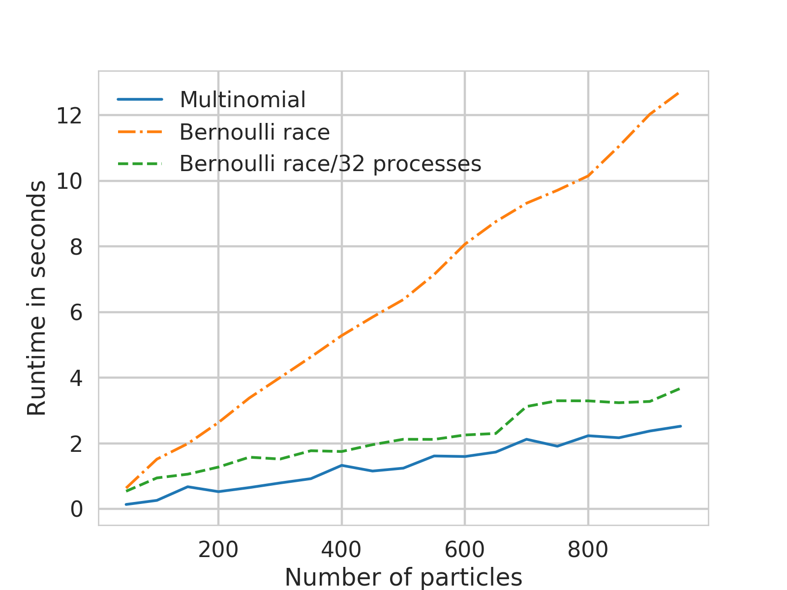
is known analytically and is Gaussian. Therefore, in this special case the rejection sampler can be avoided. This will not usually be the case, hence we use the rejection sampler for our simulation. However, this will significantly speed up the state transition. In FigureΒ 4 we compare the run-time of both, the RWPF and BRPF for different numbers of particles. In scenario (a) we use the cheap transition. Here the RWPF is very efficient. However, in scenario (b), which we also show in the main paper, where sampling from the transition is more expensive, we can implement the BRPF with the same run-time as the RWPF.
Refer to caption
(a) Simulating from known Gaussian.
Refer to caption
(b) Rejection Sampler.
Figure 4: Comparing the run-time for different implementation for the proposal q(β‹…βˆ£x,y)q(\cdot\mid x,y). In case (a) the Gaussian proposal is sampled using a naΓ―ve implementation. In (b) we use a rejection sampler proposing from the state transition.

B.2 Sine diffusion: run-time

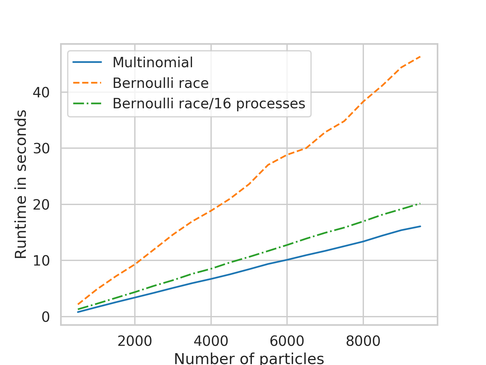
Here we compare the run-time for the RWPF and BRPF for the sine diffusion state space model. As pointed out in the main text, the BRPF is slower when implemented sequentially, but we observe in FigureΒ 5 that the difference almost completely vanishes when use a parallel implementation with 16 processes.
Refer to caption
Figure 5: Comparison of the run-time for RWPF and BRPF for sine diffusion state space model. For BRPF we show a sequential and a parallel implementation with 16 cores. For all algorithms we show wall-clock time for number of particles N𝑁N.

Appendix C Cox Process inference

To further demonstrate the range of possible application and for further illustration of the Bernoulli race particle filter, we consider another application of the BRPF to a Cox process whose intensity function is governed by a Gaussian process that is normalized through a sigmoid function. The underlying Gaussian process is modelled as a Gauss–Markov process, allowing us to perform inference sequentially as done by [li2018sequential] based on models of [christensen2012forecasting, adams2009tractable].

C.1 Likelihood and Estimation

We assume the latent Gaussian process to evolve according to the Ornstein–Uhlenbeck process

d​Xt=A​Xt​d​t+h​d​Btt∈[0,𝒯],formulae-sequence𝑑subscript𝑋𝑑𝐴subscriptπ‘‹π‘‘π‘‘π‘‘β„Žπ‘‘subscript𝐡𝑑𝑑0𝒯dX_{t}=AX_{t}dt+hdB_{t}\qquad t\in[0,\mathcal{T}], (21)

where (Bt)t∈[0,𝒯]subscriptsubscript𝐡𝑑𝑑0𝒯(B_{t})_{t\in[0,\mathcal{T}]} denotes a Brownian motion from 00 to 𝒯𝒯\mathcal{T}. We will describe the structural assumptions on A𝐴A and hβ„Žh in more detail below. Denote the observed data by s1:nβŠ‚[0,𝒯]subscript𝑠:1𝑛0𝒯s_{1:n}\subset[0,\mathcal{T}], where n𝑛n is the number of observations. We model the data by a Cox process with intensity function

λ​(t)=σ​(X1,t)=Ξ»max1+exp⁑(βˆ’X1,t)=Ξ»max​exp⁑(X1,t)1+exp⁑(X1,t),πœ†π‘‘πœŽsubscript𝑋1𝑑subscriptπœ†max1subscript𝑋1𝑑subscriptπœ†maxsubscript𝑋1𝑑1subscript𝑋1𝑑\lambda(t)=\sigma(X_{1,t})=\frac{\lambda_{\mathrm{max}}}{1+\exp(-X_{1,t})}=\lambda_{\mathrm{max}}\frac{\exp(X_{1,t})}{1+\exp(X_{1,t})},

where (X1,t)t∈[0,𝒯]subscriptsubscript𝑋1𝑑𝑑0𝒯(X_{1,t})_{t\in[0,\mathcal{T}]} is the first coordinate of the SDE (21) introduced before. The likelihood function of the Cox process conditional on the intensity is Poisson with

p​(s1:n∣λ,𝒯)=exp⁑(βˆ’βˆ«0𝒯λ​(s)​𝑑s)β€‹βˆi=1nλ​(si).𝑝conditionalsubscript𝑠:1π‘›πœ†π’―superscriptsubscript0π’―πœ†π‘ differential-d𝑠superscriptsubscriptproduct𝑖1π‘›πœ†subscript𝑠𝑖p(s_{1:n}\mid\lambda,\mathcal{T})=\exp\left(-\int_{0}^{\mathcal{T}}\lambda(s)ds\right)\prod_{i=1}^{n}\lambda(s_{i}). (22)

The likelihood is clearly intractable due to the integral which involves the latent Gaussian process. To implement a particle filter for sequential inference we need to find an unbiased coin with probability proportional to the integral in (22). For any interval [t0,t1]βŠ‚[0,𝒯]subscript𝑑0subscript𝑑10𝒯[t_{0},t_{1}]\subset[0,\mathcal{T}] we can find an estimator for exp⁑(βˆ’βˆ«t0t1λ​(s)​𝑑s)superscriptsubscriptsubscript𝑑0subscript𝑑1πœ†π‘ differential-d𝑠\exp(-\int_{t_{0}}^{t_{1}}\lambda(s)ds) by observing that for U∼Unif​[t0,t1]similar-toπ‘ˆUnifsubscript𝑑0subscript𝑑1U\sim\mathrm{Unif}[t_{0},t_{1}] and a fixed process X=(Xt)t∈[t0,t1]𝑋subscriptsubscript𝑋𝑑𝑑subscript𝑑0subscript𝑑1X=(X_{t})_{t\in[t_{0},t_{1}]} we have

𝔼​[λ​(U)∣X=x]𝔼delimited-[]conditionalπœ†π‘ˆπ‘‹π‘₯\displaystyle\mathbb{E}\left[\lambda(U)\mid X=x\right] =∫t0t1λ​(s)t1βˆ’t0​𝑑sabsentsuperscriptsubscriptsubscript𝑑0subscript𝑑1πœ†π‘ subscript𝑑1subscript𝑑0differential-d𝑠\displaystyle=\int_{t_{0}}^{t_{1}}\frac{\lambda(s)}{t_{1}-t_{0}}ds
=1t0βˆ’t1β€‹βˆ«t0t111+exp⁑(βˆ’xs)​𝑑sabsent1subscript𝑑0subscript𝑑1superscriptsubscriptsubscript𝑑0subscript𝑑111subscriptπ‘₯𝑠differential-d𝑠\displaystyle=\frac{1}{t_{0}-t_{1}}\int_{t_{0}}^{t_{1}}\frac{1}{1+\exp(-x_{s})}ds

and hence, if V∼Unif​[0,1]similar-to𝑉Unif01V\sim\mathrm{Unif}[0,1] independent of all other random variables, we obtain

P​(V≀λ​(U)∣X=x)=∫t0t1λ​(s)t1βˆ’t0​𝑑s.𝑃𝑉conditionalπœ†π‘ˆπ‘‹π‘₯superscriptsubscriptsubscript𝑑0subscript𝑑1πœ†π‘ subscript𝑑1subscript𝑑0differential-d𝑠P\left(V\leq\lambda(U)\mid X=x\right)=\int_{t_{0}}^{t_{1}}\frac{\lambda(s)}{t_{1}-t_{0}}ds.

Now sample K∼Pois​(Ξ»max​(t1βˆ’t0))similar-to𝐾Poissubscriptπœ†maxsubscript𝑑1subscript𝑑0K\sim\mathrm{Pois}(\lambda_{\mathrm{max}}(t_{1}-t_{0})), then an unbiased coin flip can be generated using

Z=∏i=1K1​{Vi≀λmaxβˆ’Ξ»β€‹(Ui)Ξ»max},𝑍superscriptsubscriptproduct𝑖1𝐾1subscript𝑉𝑖subscriptπœ†maxπœ†subscriptπ‘ˆπ‘–subscriptπœ†maxZ=\prod_{i=1}^{K}1\left\{V_{i}\leq\frac{\lambda_{\mathrm{max}}-\lambda(U_{i})}{\lambda_{\mathrm{max}}}\right\},

where 1​{A}1𝐴1\{A\} denotes the indicator function of the set A𝐴A. This estimator is indeed unbiased as can be seen by

𝔼​[Z]=𝔼​[∏i=1K1​{Vi≀λmaxβˆ’Ξ»β€‹(Ui)Ξ»max}∣X=x]𝔼delimited-[]𝑍𝔼delimited-[]conditionalsuperscriptsubscriptproduct𝑖1𝐾1subscript𝑉𝑖subscriptπœ†maxπœ†subscriptπ‘ˆπ‘–subscriptπœ†max𝑋π‘₯\displaystyle\mathbb{E}\left[Z\right]=\mathbb{E}\left[\prod_{i=1}^{K}1\left\{V_{i}\leq\frac{\lambda_{\mathrm{max}}-\lambda(U_{i})}{\lambda_{\mathrm{max}}}\right\}\mid X=x\right]
=eβˆ’Ξ»max​(t1βˆ’t0)β€‹βˆ‘k=0∞(Ξ»max​(t1βˆ’t0))kk!β€‹βˆi=1k𝔼​[1​{Vi≀λmaxβˆ’Ξ»β€‹(Ui)Ξ»max}∣K=k,X=x]absentsuperscript𝑒subscriptπœ†maxsubscript𝑑1subscript𝑑0superscriptsubscriptπ‘˜0superscriptsubscriptπœ†maxsubscript𝑑1subscript𝑑0π‘˜π‘˜superscriptsubscriptproduct𝑖1π‘˜π”Όdelimited-[]formulae-sequenceconditional1subscript𝑉𝑖subscriptπœ†maxπœ†subscriptπ‘ˆπ‘–subscriptπœ†maxπΎπ‘˜π‘‹π‘₯\displaystyle=e^{-\lambda_{\mathrm{max}}(t_{1}-t_{0})}\sum_{k=0}^{\infty}\frac{\left(\lambda_{\mathrm{max}}(t_{1}-t_{0})\right)^{k}}{k!}\prod_{i=1}^{k}\mathbb{E}\left[1\left\{V_{i}\leq\frac{\lambda_{\mathrm{max}}-\lambda(U_{i})}{\lambda_{\mathrm{max}}}\right\}\mid K=k,X=x\right]
=eβˆ’Ξ»max​(t1βˆ’t0)β€‹βˆ‘k=0∞λmaxk​(t1βˆ’t0)kk!​(∫t0t1Ξ»maxβˆ’Ξ»β€‹(s)Ξ»max​(t1βˆ’t0)​𝑑s)kabsentsuperscript𝑒subscriptπœ†maxsubscript𝑑1subscript𝑑0superscriptsubscriptπ‘˜0superscriptsubscriptπœ†maxπ‘˜superscriptsubscript𝑑1subscript𝑑0π‘˜π‘˜superscriptsuperscriptsubscriptsubscript𝑑0subscript𝑑1subscriptπœ†maxπœ†π‘ subscriptπœ†maxsubscript𝑑1subscript𝑑0differential-dπ‘ π‘˜\displaystyle=e^{-\lambda_{\mathrm{max}}(t_{1}-t_{0})}\sum_{k=0}^{\infty}\frac{\lambda_{\mathrm{max}}^{k}\left(t_{1}-t_{0}\right)^{k}}{k!}\left(\int_{t_{0}}^{t_{1}}\frac{\lambda_{\mathrm{max}}-\lambda(s)}{\lambda_{\mathrm{max}}(t_{1}-t_{0})}ds\right)^{k}
=eβˆ’Ξ»max​(t1βˆ’t0)β€‹βˆ‘k=0∞(∫t0t1Ξ»maxβˆ’Ξ»β€‹(s)​d​s)kk!​λmaxkabsentsuperscript𝑒subscriptπœ†maxsubscript𝑑1subscript𝑑0superscriptsubscriptπ‘˜0superscriptsuperscriptsubscriptsubscript𝑑0subscript𝑑1subscriptπœ†maxπœ†π‘ π‘‘π‘ π‘˜π‘˜superscriptsubscriptπœ†maxπ‘˜\displaystyle=e^{-\lambda_{\mathrm{max}}(t_{1}-t_{0})}\sum_{k=0}^{\infty}\frac{\left(\int_{t_{0}}^{t_{1}}\lambda_{\mathrm{max}}-\lambda(s)ds\right)^{k}}{k!\lambda_{\mathrm{max}}^{k}}
=eβˆ’Ξ»max​(t1βˆ’t0)​eΞ»max​(t1βˆ’t0)​exp⁑(βˆ’βˆ«t0t1λ​(s)​𝑑s)absentsuperscript𝑒subscriptπœ†maxsubscript𝑑1subscript𝑑0superscript𝑒subscriptπœ†maxsubscript𝑑1subscript𝑑0superscriptsubscriptsubscript𝑑0subscript𝑑1πœ†π‘ differential-d𝑠\displaystyle=e^{-\lambda_{\mathrm{max}}(t_{1}-t_{0})}e^{\lambda_{\mathrm{max}}(t_{1}-t_{0})}\exp\left(-\int_{t_{0}}^{t_{1}}\lambda(s)ds\right)
=exp⁑(βˆ’βˆ«t0t1λ​(s)​𝑑s).absentsuperscriptsubscriptsubscript𝑑0subscript𝑑1πœ†π‘ differential-d𝑠\displaystyle=\exp\left(-\int_{t_{0}}^{t_{1}}\lambda(s)ds\right).

To implement the Bernoulli race particle filter we sample from the prior, which can be done exactly, as seen in the next section. As we are sampling from the prior the particle weights just depend on the observation likelihood. Suppose the particle filter is at current time t0subscript𝑑0t_{0} and we propose to move to t1=t0+Δ​tsubscript𝑑1subscript𝑑0Δ𝑑t_{1}=t_{0}+\Delta t. Let (X1,t1k),k=1,…,Nformulae-sequencesuperscriptsubscript𝑋1subscript𝑑1π‘˜π‘˜1…𝑁(X_{1,t_{1}}^{k}),k=1,\ldots,N denote a proposed particle path. Then the weight is given by

g​(si:si∈[t0,t1]∣Xk)=exp⁑(βˆ’βˆ«t0t1Ξ»k​(s)​𝑑s)β€‹βˆi:si∈[t0,t1]λ​(sik),𝑔conditionalsubscript𝑠:𝑖subscript𝑠𝑖subscript𝑑0subscript𝑑1superscriptπ‘‹π‘˜superscriptsubscriptsubscript𝑑0subscript𝑑1superscriptπœ†π‘˜π‘ differential-d𝑠subscriptproduct:𝑖subscript𝑠𝑖subscript𝑑0subscript𝑑1πœ†subscriptsuperscriptπ‘ π‘˜π‘–g(s_{i\colon s_{i}\in[t_{0},t_{1}]}\mid X^{k})=\exp\left(-\int_{t_{0}}^{t_{1}}\lambda^{k}(s)ds\right)\prod_{i\colon s_{i}\in[t_{0},t_{1}]}\lambda(s^{k}_{i}),

where

Ξ»k​(s)=exp⁑(X1,sk)1+exp⁑(X1,sk).superscriptπœ†π‘˜π‘ superscriptsubscript𝑋1π‘ π‘˜1superscriptsubscript𝑋1π‘ π‘˜\lambda^{k}(s)=\frac{\exp(X_{1,s}^{k})}{1+\exp(X_{1,s}^{k})}.

In the notation of Section 4 we have

ct1ksuperscriptsubscript𝑐subscript𝑑1π‘˜\displaystyle c_{t_{1}}^{k} =∏i:si∈[t0,t1]Ξ»k​(si),absentsubscriptproduct:𝑖subscript𝑠𝑖subscript𝑑0subscript𝑑1superscriptπœ†π‘˜subscript𝑠𝑖\displaystyle=\prod_{i\colon s_{i}\in[t_{0},t_{1}]}\lambda^{k}(s_{i}),
bt1ksuperscriptsubscript𝑏subscript𝑑1π‘˜\displaystyle b_{t_{1}}^{k} =exp⁑(βˆ’βˆ«t0t1Ξ»k​(s)​𝑑s).absentsuperscriptsubscriptsubscript𝑑0subscript𝑑1superscriptπœ†π‘˜π‘ differential-d𝑠\displaystyle=\exp\left(-\int_{t_{0}}^{t_{1}}\lambda^{k}(s)ds\right).

To implement the estimator Z^^𝑍\hat{Z}, we need to be able to simulate a bridge from the stochastic differential equation (21). Since the process at hand is analytically tractable, exact sampling from the bridge is straightforward, see e.g. [bladt2016simulation] using the quantities computed below.

C.2 Ornstein–Uhlenbeck Prior

In this section we provide further details on the assumptions on the Gaussian process and show how we can sample the state transition. We assume the prior distribution on the latent space is given by the Ornstein–Uhlenbeck process (21), that is

d​Xt=A​Xt​d​t+h​d​Btt∈[0,𝒯].formulae-sequence𝑑subscript𝑋𝑑𝐴subscriptπ‘‹π‘‘π‘‘π‘‘β„Žπ‘‘subscript𝐡𝑑𝑑0𝒯dX_{t}=AX_{t}dt+hdB_{t}\qquad t\in[0,\mathcal{T}].

For A𝐴A and hβ„Žh we take the values

A𝐴\displaystyle A =[010ΞΈ],h=[0Οƒ]formulae-sequenceabsentdelimited-[]010πœƒβ„Ždelimited-[]0𝜎\displaystyle=\left[\begin{array}[]{cc}0&1\\ 0&\theta\end{array}\right],\quad h=\left[\begin{array}[]{c}0\\ \sigma\end{array}\right]

where ΞΈπœƒ\theta is a negative real value. The process can be written as a differential equation with random velocity following a mean reverting real-valued Ornstein–Uhlenbeck process,

(d​X1,td​X2,t)=[010ΞΈ]​(X1,tX2,t)​d​t+(0Οƒ)​d​Wt.matrix𝑑subscript𝑋1𝑑𝑑subscript𝑋2𝑑matrix010πœƒmatrixsubscript𝑋1𝑑subscript𝑋2𝑑𝑑𝑑matrix0πœŽπ‘‘subscriptπ‘Šπ‘‘\displaystyle\begin{pmatrix}dX_{1,t}\\ dX_{2,t}\\ \end{pmatrix}=\begin{bmatrix}0&1\\ 0&\theta\\ \end{bmatrix}\begin{pmatrix}X_{1,t}\\ X_{2,t}\\ \end{pmatrix}dt+\begin{pmatrix}0\\ \sigma\end{pmatrix}dW_{t}.

This can be written as

d​X1,t𝑑subscript𝑋1𝑑\displaystyle dX_{1,t} =X2,t​d​tabsentsubscript𝑋2𝑑𝑑𝑑\displaystyle=X_{2,t}dt
d​X2,t𝑑subscript𝑋2𝑑\displaystyle dX_{2,t} =θ​X2,t​d​t+σ​d​Bt.absentπœƒsubscript𝑋2π‘‘π‘‘π‘‘πœŽπ‘‘subscript𝐡𝑑\displaystyle=\theta X_{2,t}dt+\sigma dB_{t}.

This is a linear Gaussian system and thus the solution can be derived analytically, see e.g. [christensen2012forecasting]. The discretized system at time s>rπ‘ π‘Ÿs>r can be simulated exactly by sampling

Xs∣(Xr=x)βˆΌπ’©β€‹(eA​(sβˆ’r)​x,eA​(sβˆ’r)​Q​(r,s)​(eA​(sβˆ’r))T),similar-toconditionalsubscript𝑋𝑠subscriptπ‘‹π‘Ÿπ‘₯𝒩superscriptπ‘’π΄π‘ π‘Ÿπ‘₯superscriptπ‘’π΄π‘ π‘Ÿπ‘„π‘Ÿπ‘ superscriptsuperscriptπ‘’π΄π‘ π‘Ÿπ‘‡X_{s}\mid(X_{r}=x)\sim\mathcal{N}\left(e^{A(s-r)x},e^{A(s-r)}Q(r,s)\left(e^{A(s-r)}\right)^{T}\right),

where

Q(r,s)=∫rsexp(βˆ’At)hhTexp(βˆ’At)Tdt.Q(r,s)=\int_{r}^{s}\exp(-At)hh^{T}\exp(-At)^{T}dt.

In order to implement the Ornstein–Uhlenbeck process we need the quantities

exp⁑(A​t)𝐴𝑑\displaystyle\exp(At) =βˆ‘k=0∞tk​Akk!.absentsuperscriptsubscriptπ‘˜0superscriptπ‘‘π‘˜superscriptπ΄π‘˜π‘˜\displaystyle=\sum_{k=0}^{\infty}t^{k}\frac{A^{k}}{k!}.

Note that

A2=[010ΞΈ]​[010ΞΈ]=[0ΞΈ0ΞΈ2]superscript𝐴2delimited-[]010πœƒdelimited-[]010πœƒdelimited-[]0πœƒ0superscriptπœƒ2A^{2}=\left[\begin{array}[]{cc}0&1\\ 0&\theta\end{array}\right]\left[\begin{array}[]{cc}0&1\\ 0&\theta\end{array}\right]=\left[\begin{array}[]{cc}0&\theta\\ \text{0}&\theta^{2}\end{array}\right]
Ak=Aβ‹…Akβˆ’1superscriptπ΄π‘˜β‹…π΄superscriptπ΄π‘˜1\displaystyle A^{k}=A\cdot A^{k-1} =[010ΞΈ]​[0ΞΈkβˆ’20ΞΈkβˆ’1]absentdelimited-[]010πœƒdelimited-[]0superscriptπœƒπ‘˜20superscriptπœƒπ‘˜1\displaystyle=\left[\begin{array}[]{cc}0&1\\ \text{0}&\theta\end{array}\right]\left[\begin{array}[]{cc}0&\theta^{k-2}\\ \text{0}&\theta^{k-1}\end{array}\right]
=[0ΞΈkβˆ’10ΞΈk]absentdelimited-[]0superscriptπœƒπ‘˜10superscriptπœƒπ‘˜\displaystyle=\left[\begin{array}[]{cc}0&\theta^{k-1}\\ \text{0}&\theta^{k}\end{array}\right]

Hence, we can compute the matrix exponential analytically

exp⁑(A​t)𝐴𝑑\displaystyle\exp(At) =βˆ‘k=0∞tkk!​Akabsentsuperscriptsubscriptπ‘˜0superscriptπ‘‘π‘˜π‘˜superscriptπ΄π‘˜\displaystyle=\sum_{k=0}^{\infty}\frac{t^{k}}{k!}A^{k}
=βˆ‘k=0∞tkk!​[0ΞΈkβˆ’10ΞΈk]absentsuperscriptsubscriptπ‘˜0superscriptπ‘‘π‘˜π‘˜matrix0superscriptπœƒπ‘˜10superscriptπœƒπ‘˜\displaystyle=\sum_{k=0}^{\infty}\frac{t^{k}}{k!}\begin{bmatrix}0&\theta^{k-1}\\ 0&\theta^{k}\\ \end{bmatrix}
=[1001]+βˆ‘k=1∞tk​θkk!​[01/ΞΈ01]absentmatrix1001superscriptsubscriptπ‘˜1superscriptπ‘‘π‘˜superscriptπœƒπ‘˜π‘˜matrix01πœƒ01\displaystyle=\begin{bmatrix}1&0\\ 0&1\end{bmatrix}+\sum_{k=1}^{\infty}\frac{t^{k}\theta^{k}}{k!}\begin{bmatrix}0&1/\theta\\ 0&1\\ \end{bmatrix}
=[1001]+[0exp⁑(θ​t)/ΞΈβˆ’1/ΞΈ0exp⁑(θ​t)βˆ’1]absentmatrix1001matrix0πœƒπ‘‘πœƒ1πœƒ0πœƒπ‘‘1\displaystyle=\begin{bmatrix}1&0\\ 0&1\end{bmatrix}+\begin{bmatrix}0&\exp(\theta t)/\theta-1/\theta\\ 0&\exp(\theta t)-1\\ \end{bmatrix}
=[1exp⁑(θ​t)/ΞΈβˆ’1/ΞΈ0exp⁑(θ​t)].absentmatrix1πœƒπ‘‘πœƒ1πœƒ0πœƒπ‘‘\displaystyle=\begin{bmatrix}1&\exp(\theta t)/\theta-1/\theta\\ 0&\exp(\theta t)\\ \end{bmatrix}.

This gives us

exp⁑(βˆ’A​t)​hπ΄π‘‘β„Ž\displaystyle\exp(-At)h =[1exp⁑(βˆ’ΞΈβ€‹t)/ΞΈβˆ’1/ΞΈ0exp⁑(βˆ’ΞΈβ€‹t)]​[0Οƒ]absentmatrix1πœƒπ‘‘πœƒ1πœƒ0πœƒπ‘‘matrix0𝜎\displaystyle=\begin{bmatrix}1&\exp(-\theta t)/\theta-1/\theta\\ 0&\exp(-\theta t)\end{bmatrix}\begin{bmatrix}0\\ \sigma\end{bmatrix}
=[σθ​exp⁑(βˆ’ΞΈβ€‹t)βˆ’Οƒ/θσ​exp⁑(βˆ’ΞΈβ€‹t)]absentmatrixπœŽπœƒπœƒπ‘‘πœŽπœƒπœŽπœƒπ‘‘\displaystyle=\begin{bmatrix}\frac{\sigma}{\theta}\exp(-\theta t)-\sigma/\theta\\ \sigma\exp(-\theta t)\end{bmatrix}

and

exp⁑(βˆ’A​t)​h​hT​exp⁑(βˆ’A​t)π΄π‘‘β„Žsuperscriptβ„Žπ‘‡π΄π‘‘\displaystyle\exp(-At)hh^{T}\exp(-At)
=[σθ​exp⁑(βˆ’ΞΈβ€‹t)βˆ’Οƒ/θσ​exp⁑(βˆ’ΞΈβ€‹t)]​[σθ​exp⁑(βˆ’ΞΈβ€‹t)βˆ’Οƒ/θσ​exp⁑(βˆ’ΞΈβ€‹t)]absentmatrixπœŽπœƒπœƒπ‘‘πœŽπœƒπœŽπœƒπ‘‘matrixπœŽπœƒπœƒπ‘‘πœŽπœƒπœŽπœƒπ‘‘\displaystyle=\begin{bmatrix}\frac{\sigma}{\theta}\exp(-\theta t)-\sigma/\theta\\ \sigma\exp(-\theta t)\end{bmatrix}\begin{bmatrix}\frac{\sigma}{\theta}\exp(-\theta t)-\sigma/\theta&\sigma\exp(-\theta t)\end{bmatrix}
=[Οƒ2ΞΈ2​(exp⁑(βˆ’ΞΈβ€‹t)βˆ’1)2Οƒ2θ​(exp⁑(βˆ’2​θ​t)βˆ’exp⁑(βˆ’ΞΈβ€‹t))Οƒ2θ​(exp⁑(βˆ’2​θ​t)βˆ’exp⁑(βˆ’ΞΈβ€‹t))Οƒ2​exp⁑(βˆ’2​θ​t)].absentmatrixsuperscript𝜎2superscriptπœƒ2superscriptπœƒπ‘‘12superscript𝜎2πœƒ2πœƒπ‘‘πœƒπ‘‘superscript𝜎2πœƒ2πœƒπ‘‘πœƒπ‘‘superscript𝜎22πœƒπ‘‘\displaystyle=\begin{bmatrix}\frac{\sigma^{2}}{\theta^{2}}\left(\exp(-\theta t)-1\right)^{2}&\frac{\sigma^{2}}{\theta}\left(\exp(-2\theta t)-\exp(-\theta t)\right)\\ \frac{\sigma^{2}}{\theta}\left(\exp(-2\theta t)-\exp(-\theta t)\right)&\sigma^{2}\exp(-2\theta t)\end{bmatrix}.

Thus

Q​(r,s)π‘„π‘Ÿπ‘ \displaystyle Q(r,s) =∫rsexp(βˆ’At)hhTexp(βˆ’At)Tdt\displaystyle=\int_{r}^{s}\exp(-At)hh^{T}\exp(-At)^{T}dt
=[∫rsΟƒ2​(exp⁑(βˆ’ΞΈβ€‹t)βˆ’1)2​𝑑t∫rsΟƒ2θ​(exp⁑(βˆ’2​θ​t)βˆ’exp⁑(βˆ’ΞΈβ€‹t))​𝑑t∫rsΟƒ2​(exp⁑(βˆ’2​θ​t)βˆ’exp⁑(βˆ’ΞΈβ€‹t)/ΞΈ)​𝑑t∫rsΟƒ2​exp⁑(βˆ’2​θ​t)​𝑑t]absentmatrixsuperscriptsubscriptπ‘Ÿπ‘ superscript𝜎2superscriptπœƒπ‘‘12differential-d𝑑superscriptsubscriptπ‘Ÿπ‘ superscript𝜎2πœƒ2πœƒπ‘‘πœƒπ‘‘differential-d𝑑superscriptsubscriptπ‘Ÿπ‘ superscript𝜎22πœƒπ‘‘πœƒπ‘‘πœƒdifferential-d𝑑superscriptsubscriptπ‘Ÿπ‘ superscript𝜎22πœƒπ‘‘differential-d𝑑\displaystyle=\begin{bmatrix}\int_{r}^{s}\sigma^{2}\left(\exp(-\theta t)-1\right)^{2}dt&\int_{r}^{s}\frac{\sigma^{2}}{\theta}\left(\exp(-2\theta t)-\exp(-\theta t)\right)dt\\ \int_{r}^{s}\sigma^{2}\left(\exp(-2\theta t)-\exp(-\theta t)/\theta\right)dt&\int_{r}^{s}\sigma^{2}\exp(-2\theta t)dt\end{bmatrix}
=[Οƒ2ΞΈ3​(βˆ’2​θ​r+eβˆ’2​θ​rβˆ’4​eβˆ’ΞΈβ€‹rβˆ’eβˆ’2​θ​s+4​eβˆ’ΞΈβ€‹s+2​θ​s)Οƒ22​θ2​(eβˆ’2​rβ€‹ΞΈβˆ’eβˆ’2​s​θ)βˆ’Οƒ2ΞΈ2​(eβˆ’rβ€‹ΞΈβˆ’eβˆ’s​θ)Οƒ22​θ2​(eβˆ’2​rβ€‹ΞΈβˆ’eβˆ’2​s​θ)βˆ’Οƒ2ΞΈ2​(eβˆ’rβ€‹ΞΈβˆ’eβˆ’s​θ)Οƒ22​θ​(eβˆ’2​rβ€‹ΞΈβˆ’eβˆ’2​s​θ)]absentmatrixsuperscript𝜎2superscriptπœƒ32πœƒπ‘Ÿsuperscript𝑒2πœƒπ‘Ÿ4superscriptπ‘’πœƒπ‘Ÿsuperscript𝑒2πœƒπ‘ 4superscriptπ‘’πœƒπ‘ 2πœƒπ‘ superscript𝜎22superscriptπœƒ2superscript𝑒2π‘Ÿπœƒsuperscript𝑒2π‘ πœƒsuperscript𝜎2superscriptπœƒ2superscriptπ‘’π‘Ÿπœƒsuperscriptπ‘’π‘ πœƒsuperscript𝜎22superscriptπœƒ2superscript𝑒2π‘Ÿπœƒsuperscript𝑒2π‘ πœƒsuperscript𝜎2superscriptπœƒ2superscriptπ‘’π‘Ÿπœƒsuperscriptπ‘’π‘ πœƒsuperscript𝜎22πœƒsuperscript𝑒2π‘Ÿπœƒsuperscript𝑒2π‘ πœƒ\displaystyle=\begin{bmatrix}\frac{\sigma^{2}}{\theta^{3}}\left(-2\theta r+e^{-2\theta r}-4e^{-\theta r}-e^{-2\theta s}+4e^{-\theta s}+2\theta s\right)&\frac{\sigma^{2}}{2\theta^{2}}\left(e^{-2r\theta}-e^{-2s\theta}\right)-\frac{\sigma^{2}}{\theta^{2}}\left(e^{-r\theta}-e^{-s\theta}\right)\\ \frac{\sigma^{2}}{2\theta^{2}}\left(e^{-2r\theta}-e^{-2s\theta}\right)-\frac{\sigma^{2}}{\theta^{2}}\left(e^{-r\theta}-e^{-s\theta}\right)&\frac{\sigma^{2}}{2\theta}\left(e^{-2r\theta}-e^{-2s\theta}\right)\end{bmatrix}

The covariance matrix for the system transition

Cov​(r,s)=eA​(sβˆ’r)​Q​(r,s)​(eA​(sβˆ’r))TCovπ‘Ÿπ‘ superscriptπ‘’π΄π‘ π‘Ÿπ‘„π‘Ÿπ‘ superscriptsuperscriptπ‘’π΄π‘ π‘Ÿπ‘‡\displaystyle\mathrm{Cov}(r,s)=e^{A(s-r)}Q(r,s)\left(e^{A(s-r)}\right)^{T}

can thus be computed analytically.

C.3 Simulation

We simulate a non-homogeneous Poisson process in the interval [0,50]050[0,50] using the intensity function

λ​(s)=2​exp⁑(βˆ’s/15)+exp⁑(βˆ’((sβˆ’25)/10)2),πœ†π‘ 2𝑠15superscript𝑠25102\lambda(s)=2\exp(-s/15)+\exp\left(-((s-25)/10)^{2}\right),

see e.g. [adams2009tractable, li2018sequential]. We run the Bernoulli race particle filter with the above specification and 303030 particles to find the intensity function on the interval [0,50]050[0,50] which is divided into 10 equispaced intervals. The result of one run is shown in FigureΒ 6. We can see that the Bernoulli race particle filter is approximating the true intensity function.
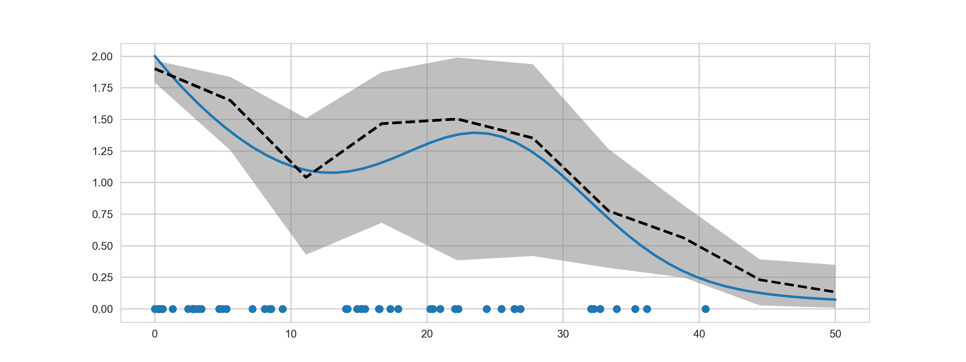
Refer to caption
Figure 6: Result of one run of the Bernoulli race particle filter using 30 particles. Arrival times of the Poisson process are shown as dots on the abscissa. The solid blue line shows the true intensity function and the dashed line shows the mean of the particle approximation at times t1,t2,…subscript𝑑1subscript𝑑2…t_{1},t_{2},\ldots. The shaded area highlights the 10% and 90% quantile of the particle approximation.