Inexact elastic shape matching in the square root normal field framework
Abstract.
This paper puts forth a new formulation and algorithm for the elastic matching problem on unparametrized curves and surfaces. Our approach combines the frameworks of square root normal fields and varifold fidelity metrics into a novel framework, which has several potential advantages over previous works. First, our variational formulation allows us to minimize over reparametrizations without discretizing the reparametrization group. Second, the objective function and gradient are easy to implement and efficient to evaluate numerically. Third, the initial and target surface may have different samplings and even different topologies. Fourth, texture can be incorporated as additional information in the matching term similarly to the fshape framework. We demonstrate the usefulness of this approach with several numerical examples of curves and surfaces.
Key words and phrases:
curve matching, surface matching, elastic shape analysis, square root normal fields, varifold distances2010 Mathematics Subject Classification:
68U05, 49Q10, 58D101. Introduction
1.1. Context.
The statistical analysis of datasets of curves and surfaces is an active research field with many applications in e.g. computer vision, robotics, and medical imaging; see [24, 4, 20] and references therein. A recurring and fundamental task is finding optimal point correspondences between given shapes (i.e., the matching or registration problem), where optimality is typically expressed in terms of an elastic deformation energy. Solving the elastic matching problem in a numerically efficient way, which scales well to high-dimensional data encountered in real-world applications, remains a major challenge to date.
1.2. Relation to previous work.
This paper draws on two lines of work: square root normal fields (SRNFs) [19, 14, 11, 12], which allow one to efficiently calculate elastic distances between parametrized shapes, and varifold distances [22, 9, 7, 18, 13], which are distances between unparametrized shapes without any elastic interpretation. For each of these frameworks, efficient numerical implementations have been developed.
1.3. Contribution.
We propose a new algorithm which combines SRNFs with varifold distances and inherits many advantages of both approaches. The key idea is to use varifold distances to relax the terminal constraint in the elastic matching problem. This bypasses the discretization of the reparametrization group, thereby eliminating the main computational burden in previous implementations of SRNF-based elastic shape matching. The resulting optimization problem is easy to implement and yields good results on some preliminary experiments on curves and surfaces. Moreover, the varifold distances allow one to match shapes with different meshes and even different topologies and to use texture information as in the fshape framework.
2. Shape analysis of curves and surfaces
2.1. Elastic shape analysis.
Elastic shape analysis operates in a Riemannian framework where infinitesimal shape deformations are measured by a Riemannian metric, which is often related to an elastic (or plastic) deformation energy; see the surveys [4, 12]. We consider parameterized shapes as elements of the Fréchet manifold of immersed hypersurfaces of a -dimensional compact manifold into . The corresponding space of unparameterized shapes is the quotient space , whose elements are denoted by . Given a -invariant weak Riemannian metric on , one defines a pseudo-distance between any two immersions and their equivalence classes by
| (1) | |||
| (2) |
Symmetry of the pseudo-distance on follows from the invariance of the metric with respect to reparametrizations. Under suitable conditions on the pseudo-distance is a distance, i.e., it separates points in the shape space of curves [17, 16] or surfaces [5].
From a numerical perspective, the challenge is to calculate the above distances and the corresponding optimizers efficiently. This minimization can be solved numerically by path straightening and geodesic shooting methods (see e.g. [10, 2]) or as in the next section by exploiting isometries to simpler spaces.
2.2. Square root normal fields.
Problem (1) simplifies considerably for certain first order Sobolev metrics [23, 25, 19, 21, 14, 11, 3]. One class of such metrics is defined using square root normal fields (SRNFs), which were introduced by Srivastava e.a. [19, 14] for planar curves and later generalized to surfaces by Jermyn e.a. [11]. The SRNF of an oriented immersed hypersurface is defined as , where is the unit normal field and the half density of . For example, the SRNF of a planar curve is given in coordinates by , where denotes rotation by 90 degrees and coordinates in subscripts denote derivatives. Similarly, the SRNF of a surface is given in coordinates as . In general, one obtains an elastic pseudo-Riemannian metric on by setting
where denotes the directional derivative of at in the direction . This pseudo-Riemannian metric is -invariant, and by construction the map is a Riemannian isometry into the flat space of square integrable vector-valued half densities. For curves one obtains a Riemannian metric by modding out translations. For surfaces the situation is more complicated, as described in [11], and the kernel of the pseudo-metric may be larger than only translations. The metric belongs to the class of first order Sobolev metrics, which have been studied in great detail [17, 16, 5].
The advantage of this construction is that the Riemannian distance of on can be approximated efficiently as follows:
| (3) |
Equality holds whenever the straight line between and is contained in the range of the map . In general, equality holds up to first order for close to because the map is a Riemannian isometry.
The approximate distance (3) descends to the quotient space as described in (2). However, (2) involves a minimization over the reparametrization group, which is computationally costly. For curves this can be solved by dynamic programming [19] or using an explicit formula [15]. For surfaces in spherical coordinates, Jermyn e.a. [11] proposed to discretize the diffeomorphism group of the two-dimensional sphere using spherical harmonics. This article puts forth an alternative method for minimization over the reparametrization group, which is based on varifold distances.
2.3. Varifold distances.
Geometric measure theory provides several embeddings of shape spaces into Banach spaces of distributions [22, 9, 7, 18, 13] with corresponding metrics. Varifold embeddings are one instance of this construction and are defined as follows (cf. [13] for details). Given a reproducing kernel Hilbert space of real-valued functions on , one associates to any immersion the varifold which satisfies
The map is reparametrization-invariant and, under suitable assumptions on the kernel of , injective [13]. Thus, one obtains a well-defined distance on the quotient space by defining for any two immersions :
From a computational point of view, these distances have explicit expressions in terms of the kernel function of and are easy to implement for discrete curves or surfaces. We will use such distances to relax the terminal constraint in the boundary value problem for geodesics on shape space, as described next.
2.4. Combining SRNFs and varifold distances.
Square root normal fields and varifold distances can be combined in an efficient matching algorithm for unparametrized shapes. This idea has been previously used in combination with large deformation models in [7, 13] and with metrics on the space of curves in [1]. The boundary value problem (2) for geodesics on can be formulated as the program
| (4) |
Relaxation using a (large) Lagrange multiplier and approximation of the elastic distance as in (3) yields
| (5) |
This program has several advantages over previous alternative formulations of the SRNF matching problem [19, 14, 11]. First, the objective function and its gradient are easy to implement and can be computed efficiently. Second, the initial and target surface may have different discretizations and even different topologies. Third, texture information can be incorporated into the varifold matching term similarly to the fshape framework [8, 6].
3. Numerical implementation and results
3.1. Algorithm.
Given a pair of curves or surfaces, the program (5) looks for a minimizer with and . Thus, the algorithm solves the registration problem and calculates the distance between the unparametrized shapes and . Note that it does, however, not provide a geodesic homotopy between these shapes. Such a homotopy can be obtained from the linear homotopy between and by (approximate) inversion of the SRNF map . For open curves this inversion is exact and easy to implement. For closed curves, the range of the SRNF map is not convex, and an approximate inverse has to be used [19]. For surfaces, this is a delicate issue [11], and to the best of our knowledge there exists no publicly available implementation for general triangulated surfaces.
3.2. Implementation.
To implement the program (5) numerically, one has to discretize the space of parametrized shapes. An advantage over [11] is that the reparametrization group does not need to be discretized. Piecewise linear curves and triangular meshes are suitable discretizations in our context, the reason being that square root normal fields and kernel-based varifold distances extend naturally to these spaces. The minimization is performed using an L-BFGS method. The gradient of the discretized energy functional (5), which is needed by the L-BFGS method, has an explicit form and can be implemented efficiently.
3.3. Curves.


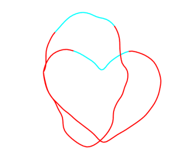
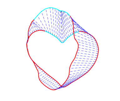
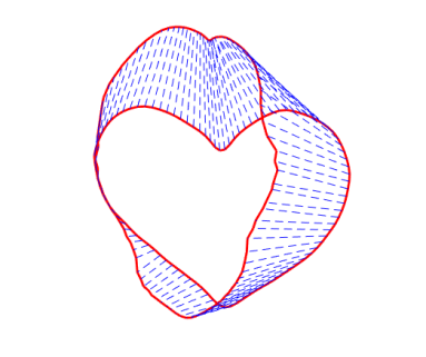
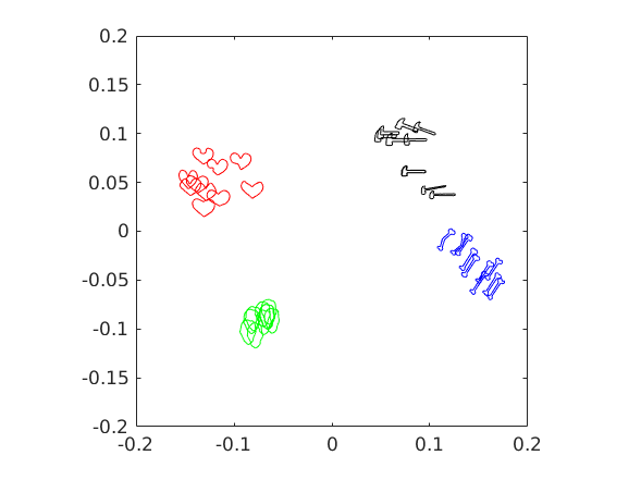
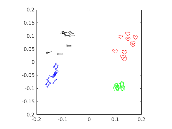
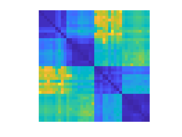
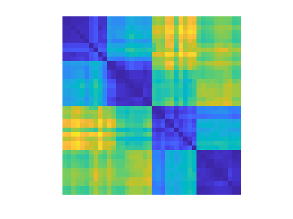
For curves, our algorithm is comparable to state of the art methods. On the Kimia dataset111Computer Vision Group at LEMS at Brown University: Database of 99 binary shapes. https://vision.lems.brown.edu/content/available-software-and-databases it produces distances and clusters which are similar to those based on dynamic programming, as shown in Fig 1. A nice feature of our algorithm, which stems from the use of varifold distances, is that the initial and target shapes are allowed to have different topologies. For example, one can match a single circle to a pair of circles, as demonstrated in Fig. 2. This is not possible using previous methods for shape matching using SRNFs or SRVTs. There are potential applications in cell division and removal of topological noise. Another feature of our algorithm is that it can account for functional data on the given shapes, as demonstrated in Fig. 3. To this aim, the varifold distance in (5) is replaced by a functional shape distance, as developed in [8, 6]. This has several applications. The functional data may be dictated by the application at hand, as e.g. in the case of texture information. An interesting alternative to be explored in future work is to use shape descriptors as functional data to guide the matching algorithm.
3.4. Surfaces.
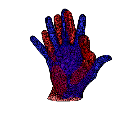
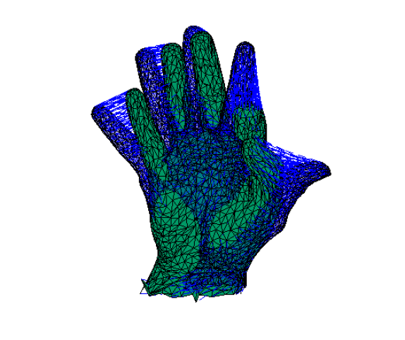
For surfaces, we obtain some promising first results and see a high potential of improvement over alternative methods. An example is presented in Fig. 4, where the optimal point correspondences between two hand postures were calculated. As the two triangulated surfaces in this experiment had different mesh connectivities, and no point-to-point correspondences were initially available, we had to initialize the optimization procedure with the template surface. After optimization using an adaptive choice of Lagrange multiplier in (5), we obtained an excellent fit of the deformed template onto the target with anatomically correct point correspondences.
References
- [1] Bauer, M., Bruveris, M., Charon, N., Møller-Andersen, J.: A relaxed approach for curve matching with elastic metrics. ESAIM COCV (2018), forthcoming
- [2] Bauer, M., Bruveris, M., Harms, P., Møller-Andersen, J.: A numerical framework for Sobolev metrics on the space of curves. SIAM J. Imaging Sci. 10(1), 47–73 (2017)
- [3] Bauer, M., Bruveris, M., Marsland, S., Michor, P.W.: Constructing reparameterization invariant metrics on spaces of plane curves. Differential Geom. Appl. 34, 139–165 (2014)
- [4] Bauer, M., Bruveris, M., Michor, P.W.: Overview of the geometries of shape spaces and diffeomorphism groups. J. Math. Imaging Vision 50(1-2), 60–97 (2014)
- [5] Bauer, M., Harms, P., Michor, P.W.: Sobolev metrics on shape space of surfaces. J. Geom. Mech. 3(4), 389–438 (2011)
- [6] Charlier, B., Charon, N., Trouvé, A.: The fshape framework for the variability analysis of functional shapes. Found. Comput. Math. 17(2), 287–357 (2017)
- [7] Charon, N., Trouvé, A.: The varifold representation of nonoriented shapes for diffeomorphic registration. SIAM J. Imaging Sci. 6(4), 2547–2580 (2013)
- [8] Charon, N., Trouvé, A.: Functional currents: a new mathematical tool to model and analyse functional shapes. J. Math. Imaging Vision 48(3), 413–431 (2014)
- [9] Glaunès, J., Qiu, A., Miller, M.I., Younes, L.: Large deformation diffeomorphic metric curve mapping. Int. J. Comput. Vis. 80(3), 317 (2008)
- [10] Huang, W., Gallivan, K.A., Srivastava, A., Absil, P.A.: Riemannian optimization for registration of curves in elastic shape analysis. J. Math. Imaging Vision 54(3), 320–343 (2016)
- [11] Jermyn, I.H., Kurtek, S., Klassen, E., Srivastava, A.: Elastic shape matching of parameterized surfaces using square root normal fields. In: European Conference on Computer Vision. pp. 804–817. Springer (2012)
- [12] Jermyn, I.H., Kurtek, S., Laga, H., Srivastava, A.: Elastic shape analysis of three-dimensional objects. Synthesis Lectures on Computer Vision 12(1), 1–185 (2017)
- [13] Kaltenmark, I., Charlier, B., Charon, N.: A general framework for curve and surface comparison and registration with oriented varifolds. In: Computer Vision and Pattern Recognition (CVPR) (2017)
- [14] Kurtek, S., Klassen, E., Gore, J.C., Ding, Z., Srivastava, A.: Elastic geodesic paths in shape space of parameterized surfaces. IEEE Trans. Pattern Anal. Mach. Intell. 34(9), 1717–1730 (2012)
- [15] Lahiri, S., Robinson, D., Klassen, E.: Precise matching of PL curves in in the square root velocity framework. Geom. Imaging Comput. 2(3), 133–186 (2015)
- [16] Mennucci, A., Yezzi, A., Sundaramoorthi, G.: Properties of Sobolev-type metrics in the space of curves. Interfaces Free Bound. 10(4), 423–445 (2008)
- [17] Michor, P.W., Mumford, D.: An overview of the Riemannian metrics on spaces of curves using the Hamiltonian approach. Appl. Comput. Harmon. Anal. 23(1), 74–113 (2007)
- [18] Roussillon, P., Glaunes, J.A.: Kernel metrics on normal cycles and application to curve matching. SIAM J. Imaging Sci. 9(4), 1991–2038 (2016)
- [19] Srivastava, A., Klassen, E., Joshi, S.H., Jermyn, I.H.: Shape analysis of elastic curves in Euclidean spaces. IEEE Trans. Pattern Anal. Mach. Intell. 33(7), 1415–1428 (2011)
- [20] Srivastava, A., Klassen, E.P.: Functional and shape data analysis. Springer (2016)
- [21] Sundaramoorthi, G., Mennucci, A., Soatto, S., Yezzi, A.: A new geometric metric in the space of curves, and applications to tracking deforming objects by prediction and filtering. SIAM J. Imaging Sci. 4(1), 109–145 (2011)
- [22] Vaillant, M., Glaunès, J.: Surface matching via currents. In: Biennial International Conference on Information Processing in Medical Imaging. pp. 381–392. Springer (2005)
- [23] Younes, L.: Computable elastic distances between shapes. SIAM J. Appl. Math. 58(2), 565–586 (1998)
- [24] Younes, L.: Shapes and diffeomorphisms, vol. 171. Springer Science & Business Media (2010)
- [25] Younes, L., Michor, P.W., Shah, J., Mumford, D.: A metric on shape space with explicit geodesics. Atti Accad. Naz. Lincei Rend. Lincei Mat. Appl. 19(1), 25–57 (2008)