Abstract

Fracture functions are parton distributions of an initial hadron in the presence of an almost collinear particle observed in the final state. They are important ingredients in QCD factorization for processes where a particle is produced diffractively. There are different fracture functions for a process in different kinematic regions. We take the production of a lepton pair combined with a diffractively produced particle in hadron collisions to discuss this. Those fracture functions can be factorized further if there are large energy scales involved. We perform one-loop calculations to illustrate the factorization in the case with the diffractively produced particle as a real photon. Evolution equations of different fracture functions are derived from our explicit calculations. They agree with expectations. These equations can be used for re-summations of large log terms in perturbative expansions.

1. Introduction

It is well-known that QCD factorization can be used to predict inclusive productions of a particle with large transverse momentum in hadron-collisions or in Semi-Inclusive DIS(SIDIS). The predictions from QCD factorizations are made in terms of parton distribution functions and parton fragmentation functions. But, if the transverse momentum $k_{\perp}$ of the produced particle is very small in hadron collisions or the particle produced in SIDIS is in target fragmentation region, the predictions with parton distribution functions and parton fragmentation functions fail, because perturbative coefficient functions in the factorization become divergent as powers of $\ln k_{\perp}$.

It has been proposed in [1] to use fracture functions to describe particle production in target fragmentation region of DIS. Experimentally, evidences of such a production have been found at HERA[2]. An one-loop calculation in [3] of SIDIS shows that QCD factorization with fracture functions can be made in the target fragmentation region in the sense that perturbatively calculable part is finite. At the moment, most information about fracture functions comes from analysis of HERA data, e.g., in [4, 5]. For hadron collisions, factorizations with fracture functions for the production of one particle combined with a lepton-pair have been shown to hold at one-loop level in [6, 7], where the produced particle is in the forward- or backward regions. We notice that fracture functions used in these works are for the case where the transverse momentum of the particle in the final state is not observed or integrated over.

Fracture functions, also called as diffractive parton distributions, are parton distributions of an initial hadron with one diffractively produced particle observed in the final state. There are different fracture functions, which can be used in different kinematic regions of a process. Taking the production of a lepton pair with large invariant mass in hadron collisions associated with a diffractively produced particle as an example, there are two kinematic regions where predictions can be made with fracture functions. One is the region in which the lepton pair is with large transverse momentum. The differential cross-section in this region can be factorized with the integrated fracture functions of partons, whose transverse momenta are integrated over. Another region is specified by the small transverse momentum of the lepton pair. In this case, the transverse momenta of partons can not be neglected, because the small transverse momentum of the lepton pair comes partly from that of partons. For this region, one needs to introduce Transverse Momentum Dependent(TMD) fracture functions. Integrated fracture functions have been defined in [8], where their asymptotic behavior has been derived for the region where the momentum fraction of the struck parton approaches its maximal value. In [9] TMD quark fracture functions have been classified for a polarized spin $1/2$ hadron in the initial state.

In this work, we discuss the factorizations for the production of lepton pair associated with a diffractively produced photon in hadron collisions in the two different kinematic regions discussed in the above. These factorizations can be proved following the proof for Drell-Yan processes in [10]. Then we study the factorization properties of integrated- and TMD quark fracture functions in the case that the produced particle is a real photon. We show that at one-loop level the integrated fracture function can be factorized with standard twist-2 parton distributions and fragmentation functions if the transverse momentum of the photon is large. We also show that the TMD quark fracture function in the impact parameter $b$ space can be factorized similarly, or with the integrated fracture function, if the parameter $b$ is small. Although we take the case of the photon, the general features of factorizations of fracture functions are the same as those in the case of a hadron. Through our results we can derive evolution equations and Collins-Soper equation of TMD fracture function. With arguments these equations are expected to be the same as those of twist-2- or TMD parton distributions. In this work we give their explicit derivations. Using these equations one can perform re-summations of large log’s in perturbative coefficient functions in collinear factorizations.

In this work we are concentrated on the case where a photon is produced diffractively. If we consider the production of a hadron instead of the photon, the factorization of differential cross-sections with fracture functions can be failed for hadron collisions as shown in [11]. For inclusive production of a single hadron in target fragmentation region of SIDIS, one can prove the factorization with fracture functions, as discussed in [8, 12]. The results about factorizations of fracture functions in a hadron are more complicated than those presented in this work. They are under preparing.

Our paper is organized as in the following: In Sect.2 we give and discuss factorization formulas with fracture functions for differential cross-section of the production of a lepton pair associated with a diffractively produced photon from hadron collisions in two kinematical regions. We also discuss the equivalence between TMD factorizations with differently defined TMD parton distributions. In Sect.3 we show at one-loop level that the integrated fracture function at large transverse momentum is factorized with parton distribution functions and fragmentation functions. A part of the evolution equation is the same as that of quark distribution as shown from our explicit result. In Sect.4 we study the TMD quark fracture function at large transverse momenta or at small impact parameter $b$. We show that at one-loop level the function can be factorized in terms of parton distribution functions and fragmentation functions if the transverse momentum of the final photon is large. We also show that in the case of the small transverse momentum the TMD fracture function in impact $b$-space is factorized with the integrated fracture function. From our results we derive the evolution equation of the renormalization scale $\mu$ and Collins-Soper equation. These equations are the same as those of TMD quark distribution as expected. Sect.5 is our summary.

2. Factorizations of Differential Cross-sections

2.1. Notations

We will use the light-cone coordinate system, in which a vector $a^{\mu}$ is expressed as $a^{\mu}=(a^{+},a^{-},\vec{a}_{\perp})=((a^{0}+a^{3})/\sqrt{2},(a^{0}-a^{3})/\sqrt{2},a^{1},a^{2})$ and $a_{\perp}^{2}=(a^{1})^{2}+(a^{2})^{2}$. We introduce two light cone vectors $n^{\mu}=(0,1,0,0)$ and $l^{\mu}=(1,0,0,0)$. The transverse metric is given by $g_{\perp}^{\mu\nu}=g^{\mu\nu}-n^{\mu}l^{\nu}-n^{\nu}l^{\mu}$.

We consider the process:

$$h_{A}(P_{A})+h_{B}(P_{B})\rightarrow\gamma^{*}(q)+\gamma(k)+X,$$ (1)

where the virtual photon will decay into an observed lepton-pair. The momenta are indicated in brackets. We take a frame in which the momenta in the process are given by:

$$P_{A}^{\mu}=(P_{A}^{+},0,0,0),\quad P_{B}^{\mu}=(0,P_{B}^{-},0,0),\quad q^{\mu}=(q^{+},q^{-},\vec{q}_{\perp}),\quad k^{\mu}=(k^{+},k^{-},\vec{k}_{\perp}),\quad q^{2}=Q^{2}.$$ (2)

We are interested in the kinematical region:

$$Q^{2}\gg\Lambda_{QCD}^{2},\quad k^{\mu}\sim Q(1,\lambda^{2},\lambda,\lambda),\quad\lambda\ll 1,$$ (3)

i.e., the observed photon is produced diffractively. We define the hadronic tensor for the process in Eq.(1) as:

$$W^{\mu\nu}=\sum_{X}\int\frac{d^{4}x}{(2\pi)^{4}}e^{iq\cdot x}\langle h_{A}(P_{A}),h_{B}(P_{B})|\bar{q}(0)\gamma^{\nu}q(0)|X,\gamma(k)\rangle\langle\gamma(k),X|\bar{q}(x)\gamma^{\mu}q(x)|h_{A}(P_{A}),h_{B}(P_{B})\rangle,$$ (4)

where the spin of the initial state is averaged and the spin of the final photon is summed. For simplicity we set the charge fraction $e_{q}$ of quarks as $1$. We consider the differential cross-section, in which only the momenta of the photon and the lepton pair are observed. It is given by:

$$(2\pi)^{3}2k^{0}\frac{d\sigma}{d^{4}qd^{3}k}=\frac{e^{4}}{12\pi sQ^{2}}W_{\mu\nu}\biggr{(}\frac{q^{\mu}q^{\nu}}{q^{2}}-g^{\mu\nu}\biggr{)}$$ (5)

with $s=2P_{A}^{+}P_{B}^{-}$.

With $Q^{2}\gg\Lambda_{QCD}^{2}$, there are effects which are calculable with perturbative QCD. One can separate or factorize nonperturbative effects from perturbative effects. The hadronic tensor takes different factorization forms in different regions of the transverse momentum $q_{\perp}$ of the lepton pair.

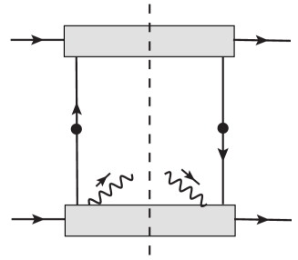
Figure 1: Tree-level diagram for the hadronic tensor.

2.2. Factorization with TMD fracture function

We discuss here the case with $q_{\perp}\sim Q\lambda$. At tree-level $W^{\mu\nu}$ receives the contribution from Fig.1, where a quark comes from hadron $h_{A}$ annihilates with an antiquark $\bar{q}$ from $h_{B}$ into the virtual photon. Since the real photon has $k_{\perp}\sim Q\lambda$ with $\lambda\rightarrow 0$, its production is nonperturbative. The description of the production is given by the fracture function indicated by the lower bubble in Fig.1. Since $q_{\perp}$ is small, one can not neglect the transverse momenta of partons.

Following general arguments for the factorization of Drell-Yan processes and SIDIS in [10, 13], the hadronic tensor can be factorized with TMD fracture function of $h_{A}$ and TMD parton distribution of $h_{B}$. We define the TMD fracture function of $h_{A}$ in impact parameter $b$-space with the transverse vector $b^{\mu}=(b^{1},b^{2})$ as:

$${\mathcal{F}}_{q/h_{A}}(x,b,\xi,k_{\perp})=\int\frac{d\lambda}{4\pi}e^{ixP_{A}^{+}\lambda}\sum_{X}\langle h_{A}(P_{A})|\bar{q}(0){\mathcal{L}}_{u}(0)\gamma^{+}|X,\gamma(k)\rangle\langle\gamma(k),X|{\mathcal{L}}^{\dagger}_{u}(\lambda n+b)q(\lambda n+b)|h_{A}(P_{A})\rangle.$$ (6)

Transforming it into the momentum space the function in the transverse momentum space is obtained:

$${\mathcal{F}}_{q/h_{A}}(x,k_{A\perp},\xi,k_{\perp})=\int\frac{d^{2}b}{(2\pi)^{2}}e^{ik_{A\perp}\cdot b}{\mathcal{F}}_{q/h_{A}}(x,b,\xi,k_{\perp}),$$ (7)

with $k^{+}=\xi P_{A}^{+}$. Here, the quark as the parton carries not only the part of the hadron momentum given by $k_{A}^{+}=xP_{A}^{+}$, but also a transverse momentum $k_{A\perp}$. The momentum fraction $x$ of the parton is in the region $1-\xi>x>0$. ${\mathcal{L}}_{u}$ is a gauge link to make the definition gauge invariant. Because $k_{A\perp}$ is not integrated over, light-cone singularities will appear if one defines TMD parton distributions with a gauge link along light-cone directions. Light-cone singularities are also called as rapidity divergences. We regularize the singularities as in [10, 13] by introducing the gauge link slightly off light-cone direction:

$${\mathcal{L}}_{u}(\xi)=P\exp\left(-ig_{s}\int_{-\infty}^{0}d\lambda u\cdot G(\lambda u+\xi)\right),$$ (8)

with $u^{\mu}=(u^{+},u^{-},0,0)$ and $u^{-}\gg u^{+}$. With the small- but finite $u^{+}$ light-cone singularities are regularized. The physical interpretation of the defined TMD fracture function is the parton distribution of $h_{A}$ in the presence of an observed photon in the final state. In the definition of Eq.(6) one should also add the gauge link of electromagnetic field to make the definition $U_{em}(1)$ gauge invariant. In this work we take the light-cone gauge $n\cdot A=0$ for QED, the electromagnetic gauge links are $1$ and can be omitted. We work only with the leading order of QED.

The TMD parton distribution of $h_{B}$ is defined similarly to Eqs.(6,7) as:

$$f_{\bar{q}/h_{B}}(y,b) = -\int\frac{d\lambda}{4\pi}e^{-iyP_{B}^{-}\lambda}\langle h_{B}(P_{B})|\bar{q}(0)\gamma^{-}{\mathcal{L}}_{v}(0){\mathcal{L}}_{v}^{\dagger}(\lambda l+b)q(\lambda l+b)|h_{B}(P_{B})\rangle,$$

$$f_{\bar{q}/h_{B}}(y,k_{B\perp}) = \int\frac{d^{2}b}{(2\pi)^{2}}e^{-ik_{B\perp}\cdot b}f_{\bar{q}/h_{B}}(x,b),$$ (9)

where the anti-quark as the parton carries the momentum $\tilde{k}_{B}^{\mu}=(0,yP_{B}^{-},k_{B\perp}^{1},k^{2}_{B\perp})$. The gauge link ${\mathcal{L}}_{v}$ here is along the direction $v^{\mu}=(v^{+},v^{-},0,0)$ and $v^{+}\gg v^{-}$. The gauge links along non-light-like directions introduce the dependence of TMD parton distribution and TMD fracture function on hadron’s energies or the parameters

$$\zeta_{v}^{2}=\frac{(2yv\cdot P_{B})^{2}}{v^{2}},\quad\zeta_{u}^{2}=\frac{(2xu\cdot P_{A})^{2}}{u^{2}}$$ (10)

respectively. The evolution of TMD fracture function and parton distribution along these parameters are governed by Collins-Soper equations, which are useful for resummations of large log’s of $k_{\perp}/Q$ or $q_{\perp}/Q$ in perturbative coefficient functions of collinear factorization.

Because the transverse momentum $q_{\perp}$ can also be generated from radiations of soft gluons, one needs not only TMD fracture function and TMD parton distribution for the factorization, but also a soft factor. The needed soft factor for the subtraction of soft gluons is defined as:

$$S(b,\rho)=\frac{1}{N_{c}}\langle 0|{\rm Tr}\left[{\mathcal{L}}^{\dagger}_{v}(b){\mathcal{L}}_{u}(b){\mathcal{L}}_{u}^{\dagger}(0){\mathcal{L}}_{v}(0)\right]|0\rangle,$$ (11)

with $\rho^{2}=(2u\cdot v)^{2}/(u^{2}v^{2})$. At tree-level one has $S^{(0)}(b,\rho)=1$. Following the studies in [10, 13], the hadronic tensor in the kinematical region $q_{\perp}\sim Q\lambda$ can be factorized as:

$$W^{\mu\nu} = -g_{\perp}^{\mu\nu}\frac{1}{N_{c}}H(Q,\zeta_{u},\zeta_{v})\int d^{2}b\ e^{-ib\cdot q_{\perp}}f_{\bar{q}/h_{B}}(y,b,\zeta_{v}){\mathcal{F}}_{q/h_{A}}(x,b,\xi,k_{\perp},\zeta_{u})S^{-1}(b,\rho)+\cdots,$$ (12)

with $q^{\mu}=(xP_{A}^{+},yP_{B}^{-},q_{\perp}^{1},q_{\perp}^{2})$. There are power corrections to the factorization formula denoted by $\cdots$. They are suppressed by powers of $\lambda$ or $\Lambda_{QCD}/Q$. $H$ is the perturbative coefficient. It is the same as that in TMD factorization of Drell-Yan process. From the explicit calculation in [14, 15], the perturbative coefficient is:

$$H = 1+\frac{\alpha_{s}C_{F}}{2\pi}\left[2\pi^{2}-4-\ln\frac{\mu^{2}}{Q^{2}}\left(1+\ln\rho^{2}\right)-\ln\rho^{2}+\frac{1}{2}\left(\ln^{2}\frac{Q^{2}}{\zeta_{v}^{2}}+\ln^{2}\frac{Q^{2}}{\zeta_{u}^{2}}\right)\right]+{\mathcal{O}}(\alpha_{s}^{2}).$$ (13)

In Eq.(12) we only give the contribution from the quark fracture function of $h_{A}$ and the TMD antiquark distribution of $h_{B}$. There are contributions from the TMD quark distribution of $h_{B}$ and the TMD antiquark fracture function of $h_{A}$. They can be obtained through transformation of charge-conjugation, i.e., by reversing the directions of quark lines in Fig.1.

In the above, the used TMD fracture function, parton distribution function are called as unsubtracted ones. They are defined with non light-cone gauge links for regularizing light-cone singularities. It is noted that the TMD fracture function here is defined with the same operators used to define TMD parton distributions, if one ignores the photon in the intermediate state in Eq.(6). There are different methods to regularize or eliminate the singularities. With different methods TMD parton distributions can be defined differently. In [16] light-cone gauge links are used to define unsubtracted TMD quark distributions. The light-cone singularities are cancelled by a soft factor which is different than the one here. In the framework of Soft Collinear Effective Theory(SCET), only light-cone gauge links are used. The light-cone singularities are regularized by the so-called $\delta$-regulators in [17] or by the $\nu$-regulators in [18]. Although TMD factorizations can be different with different TMD parton distributions, they are equivalent to each other. In the below we discuss the equivalence with Drell-Yan processes as an example, i.e., the process in Eq.(1) without the real photon in the final state.

The unsubtracted TMD quark distribution of $h_{A}$ with non light-cone gauge links is similar to Eq.(6):

$$f_{q/h_{A}}(x,b,\zeta_{u})=\int\frac{d\lambda}{4\pi}e^{ixP_{A}^{+}\lambda}\langle h_{A}(P_{A})|\bar{q}(0){\mathcal{L}}_{u}(0)\gamma^{+}{\mathcal{L}}^{\dagger}_{u}(\lambda n+b)q(\lambda n+b)|h_{A}(P_{A})\rangle,$$ (14)

and the unsubtracted antiquark distribution $f_{\bar{q}/h_{B}}$ of $h_{B}$ is defined in Eq.(9). It depends on the parameter $\zeta_{v}$. With the defined soft factor in Eq.(11) we can define the subtracted TMD parton distribution as:

$$q(x,b,\zeta_{u},\rho)=\frac{f_{q/h_{A}}(x,b,\zeta_{u})}{\sqrt{S(b,\rho)}},\quad\bar{q}(x,b,\zeta_{v},\rho)=\frac{f_{\bar{q}/h_{B}}(x,b,\zeta_{v})}{\sqrt{S(b,\rho)}}.$$ (15)

With these subtracted distributions, the hadronic tensor of Drell-Yan processes in the region of small $q_{\perp}$ is factorized as[13]:

$$W^{\mu\nu}=-g_{\perp}^{\mu\nu}\frac{1}{N_{c}}H(Q,\zeta_{u},\zeta_{v})\int d^{2}b\ e^{-ib\cdot q_{\perp}}q(x,b,\zeta_{u},\rho)\bar{q}(y,b,\zeta_{v},\rho)+\cdots,$$ (16)

with the same perturbative coefficient $H$ as given before. It should be noted that here the light-cone singularities in the TMD quark- and TMD anti-quark distributions are regularized independently, i.e., $\zeta_{u}$ and $\zeta_{v}$ are independent parameters. The parameter $\rho$ from the soft factor is fixed by $\zeta_{u}\zeta_{v}=\rho Q^{2}$.

In [16] a definition of the subtracted TMD quark distribution is given by taking the light-cone gauge link in the unsubtracted one. The subtracted one is divided with a different soft-factor than that in Eq.(11). The used soft factor is defined as a combination of different products of four gauge links. The light-cone singularity is cancelled by the soft factor. However, the soft factor contains gauge links along non-light-cone directions, characterized by the rapidity $y_{n}$. In the limit $y_{n}\rightarrow\pm\infty$, light-cone singularity appears. Therefore, the introduced TMD quark distribution in [16], denoted as $q_{J}(x,b,\zeta_{c})$, depends on the parameter $\zeta_{c}$:

$$\zeta_{c}^{2}=2(xP_{A}^{+})^{2}e^{-2y_{n}}.$$ (17)

Although the two subtracted distributions $q$ and $q_{J}$ are different, they have the same soft divergences. Therefore, the difference between the two distributions can be calculated perturbatively. From explicit results in [19] we can derive the relation between the two distributions at one-loop:

$$q(x,b,\zeta_{u},\rho)=C(b,\zeta_{u},\rho,\zeta_{c})q_{J}(x,b,\zeta_{c}),$$ (18)

with the perturbative coefficient as:

$$C(b,\zeta_{u},\rho,\zeta_{c})=1+\frac{\alpha_{s}C_{F}}{2\pi}\biggr{[}-\frac{1}{2}\ln^{2}\frac{\zeta_{u}^{2}}{\mu^{2}}-\ln\frac{\zeta_{u}^{2}}{\rho\zeta_{c}^{2}}\ln\frac{\mu^{2}b^{2}e^{2\gamma}}{4}+\ln\frac{\zeta_{u}^{2}}{\mu^{2}}-2-\frac{\pi^{2}}{2}\biggr{]}+{\mathcal{O}}(\alpha_{s}^{2}),$$ (19)

where $\gamma$ is Euler constant. Such a relation is also expected in the case of TMD fracture functions.

The factorization with TMD parton distributions in [16] is then given as:

$$W^{\mu\nu}=-g_{\perp}^{\mu\nu}\frac{1}{N_{c}}H_{J}(Q)\int d^{2}b\ e^{-ib\cdot q_{\perp}}q_{J}(x,b,\zeta_{c})\bar{q}_{J}(y,b,\zeta_{\bar{c}})+\cdots.$$ (20)

In the above the parameter $\zeta_{\bar{c}}$ in the anti-quark distribution $\bar{q}_{J}$, corresponding to $\zeta_{c}$ in $q_{J}$, is not independent. It is given as $2(yP_{B}^{-})^{2}e^{2y_{n}}$. This results in that the perturbative coefficient $H_{J}(Q)$ does not depend on $y_{n}$ or is free from light-cone singularities.

In the factorization given in Eq.(16) the parameter $\zeta_{u}$ and $\zeta_{v}$ are independent. If we take $\zeta_{u}=\zeta_{c}$ and $\zeta_{v}=\zeta_{\bar{c}}$, and express the TMD parton distributions in Eq.(16) with those defined in [16] by using Eq.(18) , we obtain the factorization formula in Eq.(20) and the perturbative coefficient $H_{J}(Q)$:

$$H_{J}(Q) = C(b,\zeta_{c},1,\zeta_{c})C(b,\zeta_{\bar{c}},1,\zeta_{\bar{c}})H(Q,\zeta_{c},\zeta_{\bar{c}})$$ (21)

$$= 1+\frac{\alpha_{s}C_{F}}{2\pi}\biggr{[}3\ln\frac{Q^{2}}{\mu^{2}}-\ln^{2}\frac{Q^{2}}{\mu^{2}}+\pi^{2}-8\biggr{]}+{\mathcal{O}}(\alpha_{s}^{2}).$$

The derived coefficient is in agreement with the coefficient given in [16]. This shows that the two factorizations with differently defined TMD parton distributions are equivalent. It is noted with $\zeta_{u}=\zeta_{c}$ and $\zeta_{u}=\zeta_{\bar{c}}$ that we have $\rho=1$ and the perturbative coefficient $C$ does not depend on $b$.

In the framework of SCET, TMD factorization of Drell-Yan processes has been studied intensively with the so-called $\delta$-regulators in [17]. Although the regulator is introduced in SCET, in full QCD it is equivalent to take light-cone gauge links to define unsubtracted TMD parton distributions and soft factor. But, the used gauge links are modified[20]. E.g., the gauge link along the $n$-direction, or ${\mathcal{L}}_{u}$ with $u^{+}=0$ is modified as:

$$P\exp\biggr{(}-ig_{s}\int^{0}_{-\infty}d\lambda n\cdot G(\lambda n+x)\biggr{)}\rightarrow P\exp\biggr{(}-ig_{s}\int^{0}_{-\infty}d\lambda n\cdot G(\lambda n+x)e^{-\delta^{+}\lambda}\biggr{)}.$$ (22)

With the small- but finite $\delta^{+}$ light-cone singularities are regularized. Because the subtracted TMD parton distributions involve a soft factor containing gauge links along the $n$- and $l$-direction, they depend on the parameters $\delta^{+}$ and $\delta^{-}$, the later regularizes the light-cone divergences in gauge links along the $l$-direction. Taking $\delta^{+}\propto\delta^{-}$, the subtracted TMD parton distributions are free from light-cone singularities. This is an advantage of the $\delta$-regulator. With it TMD parton distribution functions have been calculated at two loop in [21].

The factorization with TMD parton distributions defined with the $\delta$-regulators takes a similar form as discussed in the above. It is equivalent to the factorization with TMD factorization defined in [16], as shown in detail in [22]. Therefore, TMD factorizations with subtracted TMD parton distributions defined in different ways discussed here are all equivalent. Although the discussed equivalence is only for TMD parton distributions, it is expected that there is also such an equivalence in the case of TMD fracture functions. In this work we will only study the properties of TMD fracture function defined at the beginning of this section.

2.3. Factorization with integrated fracture function

We consider here the case that the transverse momentum of the lepton pair is large, e.g., $q_{\perp}\gg\lambda Q$. In this case the large $q_{\perp}$ is generated by hard radiations of partons. Therefore, one can neglect transverse momenta of incoming partons. This results in that one can use collinear factorization. In this kinematical region, the hadronic tensor at leading power is factorized as:

$$W^{\mu\nu} = \int dx_{A}dx_{B}\sum_{a,b}w_{ab}^{\mu\nu}(x_{A}P_{A},x_{B}P_{B},q)F_{a/h_{A}}(x_{A},\xi,k_{\perp})f_{b/h_{B}}(x_{B}),$$ (23)

where the sum is over all possible partons. $w^{\mu\nu}$ can be calculated with perturbation theory. $f_{b/B}$ is the standard parton distribution at twist-2, whose definition is given in [23]. $F_{a}$ is the fracture function of $h_{A}$. $w_{ab}^{\mu\nu}$ can be calculated with perturbation theory. At leading order they are determined by the tree-level partonic process $a+b\rightarrow\gamma^{*}+c$. We will only discuss the quark fracture function $F_{q}$ here, because of that it corresponds to the TMD fracture function introduced in the previous subsection.

The quark fracture function appearing in Eq.(23) is defined in [8] as:

$$F_{q/h_{A}}(x,\xi,k_{\perp})=\int\frac{d\lambda}{4\pi}e^{ixP_{A}^{+}\lambda}\sum_{X}\langle h_{A}(P_{A})|\bar{q}(0){\mathcal{L}}_{n}(0)\gamma^{+}|X,\gamma(k)\rangle\langle\gamma(k),X|{\mathcal{L}}_{n}^{\dagger}(\lambda n)q(\lambda n)|h_{A}(P_{A})\rangle.$$ (24)

It is noted that in the above the transverse momentum of the quark as a parton is integrated over. Because of this, the gauge links along the direction $n^{\mu}=(0,1,0,0)$ are used. With this definition there can be light-cone singularities in different contributions to $F_{q}$, but the sum is free from the singularities.

3. Factorization of Integrated Fracture Function

In this section we study the factorization of the integrated fracture function. If the observed photon in the final state has large transverse momentum, i.e., $k_{\perp}\gg\Lambda_{QCD}$, the integrated fracture function has a perturbatively calculable part. This part can be separated. The expected factorization takes the form:

$$F_{q/h_{A}}(x,\xi,k_{\perp})=\sum_{a}\int\frac{dy}{y}f_{a/h_{A}}(y)\biggr{[}{\mathcal{H}}_{a}(x/y,\xi/y,k_{\perp})+\sum_{b}\int\frac{dz}{z}D_{b}(z){\mathcal{H}}_{ab}(x/y,\xi/(yz),k_{\perp}/\sqrt{z})\biggr{]},$$ (25)

where the sum over $a$ or $b$ is the sum over all possible partons in QCD, including the contributions with the parton $a$ as a quark whose flavor is different than that of $q$ in $F_{q/h_{A}}$. ${\mathcal{H}}_{a}$ and ${\mathcal{H}}_{ab}$ are perturbative coefficient functions. $f_{a/h_{A}}$ is the twist-2 parton distribution of $h_{A}$. $D_{a}$ is the fragmentation function of a parton $a$ decaying into a photon. At one loop level, only ${\mathcal{H}}_{q,g}$ and ${\mathcal{H}}_{qg}$ are nonzero. The coefficient functions ${\mathcal{H}}_{a}$ and ${\mathcal{H}}_{ab}$, where the parton $a$ has the flavor other than that of $q$, will become nonzero beyond one-loop level.

At tree-level, i.e., at the order ${\mathcal{O}}(\alpha_{s}^{0})$, only ${\mathcal{H}}_{q}$ is nonzero. It is the same as the integrated quark fracture function of a quark at the order:

$$F_{q/q}^{(0)}(x,\xi,k_{\perp})={\mathcal{H}}^{(0)}_{q}(x,\xi,k_{\perp})=2e^{2}\delta(1-x-\xi)\frac{1}{k_{\perp}^{2}}\biggr{(}\gamma(\xi)-\frac{\epsilon}{2}\xi^{2}\biggr{)}.$$ (26)

The function $\gamma(\xi)$ is defined as:

$$\gamma(\xi)=1+(1-\xi)^{2},$$ (27)

which will be often used in our work. At one-loop, the perturbative coefficient functions receive contributions from Fig.2, Fig.3 and Fig.4. The one-loop correction of ${\mathcal{H}}_{q}$ is from diagrams given in Fig.2 and Fig.3. The diagrams in Fig.4 give contributions to ${\mathcal{H}}_{g}$ and ${\mathcal{H}}_{gq}$. In calculations of Fig.2 and Fig.3 we will have U.V. divergences represented by poles in $\epsilon=4-d$. Terms with U.V. poles are subtracted. There are collinear- and I.R. divergences. The I.R. divergences will be cancelled in the final results. The collinear divergences will be factorized into $f_{q/h_{A}}$ so that ${\mathcal{H}}^{(1)}_{q}$ is finite. Besides these singularities, there are light-cone singularities. They will also be cancelled because the transverse momentum of the parton is integrated here.

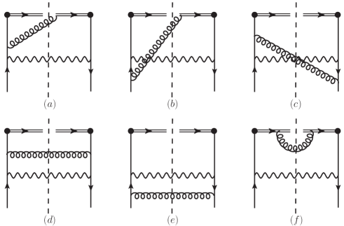
Figure 2: Diagrams for the fracture function in the case of large transverse momenta. Double lines represent gauge links. Self-energy diagrams and complex conjugated diagrams should be included.

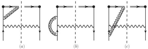
Figure 3: One-loop diagrams for the fracture function. Double lines represent gauge links. Self-energy diagrams and complex conjugated diagrams of the diagrams are not given here.

We first look at the contributions from Fig.2 and Fig.3. They are one-loop corrections of fracture function $F_{q/q}$ of an initial quark. The contributions from those diagrams, where one gluon is attached to gauge links along the direction $n$, have light-cone singularities. But they are cancelled in the sum. In the sum of the contributions from Fig.2a and Fig.3a and the sum of Fig.2b and Fig.3c there is no light-cone singularity:

$$F_{q/q}\Big{|}_{2a+3a} = \frac{e^{2}\alpha_{s}C_{F}}{\pi k_{\perp}^{2}}\gamma(\xi)\Biggl{\{}\left(\delta(z)+\frac{x}{\bar{\xi}(z)_{+}}\right)\ln\frac{\mu^{2}}{k_{\perp}^{2}}+\delta(z)(\ln\xi+2)+\frac{x}{\bar{\xi}(z)_{+}}\ln\xi\bar{\xi}^{2}-\left(\frac{\ln xz}{z}\right)_{+}\frac{x}{\bar{\xi}}\Biggr{\}},$$

$$F_{q/q}\Big{|}_{2b+3c} = \frac{e^{2}\alpha_{s}C_{F}}{\pi k_{\perp}^{2}}\Biggl{\{}\left(-\frac{2}{\epsilon_{c}}+\ln\frac{k_{\perp}^{2}}{\tilde{\mu}_{c}^{2}}\right)\left[\delta(z)\left(\gamma(\xi)\ln\bar{\xi}+2-\xi\right)+\xi+\frac{\gamma(\xi)}{(z)_{+}}-2\right]$$ (28)

$$+\delta(z)\Biggl{[}\frac{1}{4}\gamma(\xi)\ln^{2}\xi+\left(\xi-2-\frac{3}{2}\gamma(\xi)\ln\bar{\xi}\right)\ln\xi+\xi^{2}\ln\bar{\xi}+2\xi-4+\frac{\pi^{2}\gamma(\xi)}{6}$$

$$+\frac{\gamma(\xi)}{2}{\rm Li}_{2}(\xi)+\frac{\gamma(\xi)}{2}{\rm Li}_{2}\left(-\bar{\xi}/\xi\right)\Biggr{]}+\left(\frac{1}{z}\right)_{+}\left[\xi^{2}+\frac{\gamma(\xi)}{2}\ln\frac{\bar{z}^{2}}{x\xi^{2}\bar{\xi}^{2}}\right]+\frac{\gamma(\xi)}{2}\left(\frac{\ln x}{z}\right)_{+}$$

$$+\gamma(\xi)\left(\frac{\ln z}{z}\right)_{+}+(2-\xi)\ln\frac{\xi\bar{\xi}}{z\bar{z}}\Biggr{\}},$$

where $\tilde{\mu}_{c}$ is given by $4\pi\mu_{c}^{2}e^{-\gamma}$ with $\mu_{c}$ as the scale associated with the collinear divergence. $z$ is given by $z=1-x-\xi$. We use the notations $\bar{u}=1-u$ to simplify the expressions. The +-distribution in the above is defined as:

$$\int_{0}^{1-\xi}dx\ t(x)\frac{1}{(1-x-\xi)_{+}}=\int_{0}^{1-\xi}dx\frac{t(x)-t(1-\xi)}{(1-x-\xi)}.$$ (29)

The contributions from other diagrams have no light-cone divergence. They are:

$$F_{q/q}\Big{|}_{3b} = \frac{e^{2}\alpha_{s}C_{F}}{\pi k_{\perp}^{2}}\delta(z)\left[\frac{1}{2}\gamma(\xi)\ln\frac{\xi\mu^{2}}{k_{\perp}^{2}}+\xi\bar{\xi}\left(\frac{2}{\epsilon_{c}}+\ln\frac{\xi\tilde{\mu}_{c}^{2}}{k_{\perp}^{2}}\right)+\frac{3}{2}\xi\bar{\xi}+1\right],$$

$$F_{q/q}\Big{|}_{2c} = \frac{e^{2}\alpha_{s}C_{F}}{\pi k_{\bot}^{2}}\left[\frac{\xi x}{\bar{z}}\left(\frac{2}{\epsilon_{c}}+\ln\frac{\tilde{\mu}_{c}^{2}}{k_{\bot}^{2}}\right)+\left(\frac{\xi x}{\bar{z}}+\frac{\bar{x}}{2}\right)\ln\frac{\xi x}{z\bar{z}^{2}}+\frac{\bar{x}}{2}\ln\frac{xz}{\xi\bar{\xi}^{2}}+\frac{\gamma(\xi)x+\xi}{\bar{\xi}\bar{z}}-\frac{\bar{z}}{\bar{\xi}}+\xi-x\right],$$

$$F_{q/q}\Big{|}_{2d} = \frac{e^{2}\alpha_{s}C_{F}}{\pi k_{\perp}^{2}\bar{\xi}^{2}}\left[\gamma(\xi)z\left(\ln\frac{\mu^{2}}{k_{\perp}^{2}}+\ln\frac{\xi\bar{\xi}^{2}}{xz}-1\right)+\xi x\right],$$

$$F_{q/q}\Big{|}_{2e} = \frac{e^{2}\alpha_{s}C_{F}}{\pi k_{\bot}^{2}}\left[-z\left(1+\frac{x^{2}}{\bar{z}^{2}}\right)\left(\frac{2}{\epsilon_{c}}+\ln\frac{\tilde{\mu}_{c}^{2}}{k_{\bot}^{2}}+\ln\frac{\xi x}{z\bar{z}^{2}}\right)+\frac{\xi\bar{\xi}}{\bar{z}}\right].$$ (30)

The contribution of Fig.2f is zero because of that the gauge links are along the direction $n$ with $n^{2}=0$. Besides the contributions from Fig.2 and Fig.3, there are corrections from external lines and the quark propagator given by:

$$F_{q/q}(x,\xi,k_{\perp})\biggr{|}_{E}=-\frac{\alpha_{s}C_{F}}{4\pi}\biggr{[}\biggr{(}-\frac{2}{\epsilon_{c}}+\ln\frac{\mu^{2}}{\tilde{\mu}_{c}^{2}}\biggr{)}+2\biggr{(}1+\ln\frac{\xi\mu^{2}}{k_{\perp}^{2}}\biggr{)}\biggr{]}F_{q}^{(0)}(x,\xi,k_{\perp}).$$ (31)

Summing all contributions, we have the divergent part of the one-loop correction:

$$F_{q/q}^{(1)}\biggr{|}_{div.}=\frac{\alpha_{s}C_{F}e^{2}}{\pi k_{\perp}^{2}}\biggr{(}-\frac{2}{\epsilon_{c}}\biggr{)}\gamma(\xi/y)\biggr{(}\frac{1+y^{2}}{(1-y)_{+}}+\frac{3}{2}\delta(1-y)\biggr{)},$$ (32)

with $y=x+\xi$. The $+$-distribution here is the standard one:

$$\int_{\xi}^{1}dy\frac{1}{(1-y)_{+}}t(y)=\int_{\xi}^{1}dy\frac{1}{1-y}(t(y)-t(1))+t(1)\ln(1-\xi).$$ (33)

Using the result of the quark distribution of a quark as the target

$$f_{q/q}(x) = \delta(1-x)+\frac{\alpha_{s}}{2\pi}\left(-\frac{2}{\epsilon_{c}}+\ln\frac{\mu^{2}}{\tilde{\mu}_{c}^{2}}\right)C_{F}\biggr{(}\frac{1+x^{2}}{(1-x)_{+}}+\frac{3}{2}\delta(1-x)\biggr{)}+{\mathcal{O}}(\alpha_{s}^{2})$$ (34)

$$= \delta(1-x)+\frac{\alpha_{s}}{2\pi}\left(-\frac{2}{\epsilon_{c}}+\ln\frac{\mu^{2}}{\tilde{\mu}_{c}^{2}}\right)P_{qq}(x)+{\mathcal{O}}(\alpha_{s}^{2}),$$

we find that the collinear divergent part of the one-loop contribution of $F_{q}$ from Fig.2 and Fig.3 can be factorized with the quark distribution function. We have then the finite perturbative coefficient:

$${\cal H}_{q}^{(1)}(x,\xi,k_{\perp}) = \frac{e^{2}\alpha_{s}C_{F}}{\pi k_{\perp}^{2}}\left\{\ln\frac{\mu^{2}}{k_{\perp}^{2}}\left[\gamma(\xi)\gamma(\bar{y}/\bar{\xi})\left(\frac{1}{(\bar{y})_{+}}-\delta(\bar{y})\ln\bar{\xi}\right)-\gamma(\xi/y)\frac{1+y^{2}}{(\bar{y})_{+}}\right]\right.$$ (35)

$$+\delta(\bar{y})\left[\gamma(\xi)\left(-3\ln\xi\ln\bar{\xi}+2\ln\bar{\xi}+\frac{1}{2}\ln^{2}\xi+{\rm Li}_{2}\left(-\frac{\bar{\xi}}{\xi}\right)+{\rm Li}_{2}(\xi)+\frac{\pi^{2}}{6}-4\right)\right.$$

$$-4\bar{\xi}\left(\ln\bar{\xi}-2\right)+\xi^{2}+\xi\bigg{]}+\gamma(\xi)\left(\frac{1}{\bar{y}}\right)_{+}\left(2\frac{\bar{y}}{\bar{\xi}}\ln\frac{x}{\xi\bar{\xi}^{2}}-\ln\frac{x^{2}}{y^{2}\bar{\xi}^{2}}+\frac{2\xi^{2}\left(xy^{2}-\bar{\xi}\right)}{y^{2}\bar{\xi}\gamma(\xi)}\right)$$

$$+\left(-\gamma(\xi)\frac{\bar{y}}{\bar{\xi}^{2}}+\bar{y}+\xi\right)\ln\frac{\bar{y}x}{\xi\bar{\xi}^{2}}+\left(2y-\xi-(y+1)\frac{x^{2}}{y^{2}}\right)\ln\frac{\xi x}{y^{2}\bar{y}}-2\bar{\xi}\ln\frac{y}{\xi\bar{\xi}}$$

$$\left.+\frac{2}{\bar{\xi}}\ln\bar{y}-2\ln\frac{y\bar{y}}{\xi\bar{\xi}}+\frac{\xi^{2}-\xi\bar{\xi}}{y}+\frac{5\bar{y}+3}{\bar{\xi}}+\frac{(\xi^{2}-3)\bar{y}}{\bar{\xi}^{2}}+\frac{\xi^{2}}{y^{2}}-3\right\}+{\cal O}(\alpha_{s}^{2}),$$

which is finite.

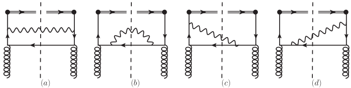
Figure 4: One-loop diagrams for the fracture function of a gluon.

The contributions from Fig.4 are those to the fracture function $F_{q/g}$ of an initial gluon. They are U.V. finite. They only contain collinear divergences represented by poles in $\epsilon_{c}=4-d$. The results are:

$$F_{q/g}\bigg{|}_{4a} = \frac{e^{2}\alpha_{s}}{2\pi k_{\perp}^{2}}\left[-\left(\bar{z}^{2}+z^{2}\right)\left(\frac{x^{2}}{\bar{z}^{2}}+1\right)\left(\frac{2}{\epsilon_{c}}+\ln\frac{\tilde{\mu}_{c}^{2}}{k_{\perp}^{2}}+\ln\frac{\xi x}{z\bar{z}^{2}}\right)+\frac{\xi\bar{x}}{\bar{z}}+4xz\right],$$

$$F_{q/g}\bigg{|}_{4b} = \frac{e^{2}\alpha_{s}}{2\pi k_{\perp}^{2}}\left[-\left(\bar{x}^{2}+x^{2}\right)\left(\frac{z^{2}}{\bar{x}^{2}}+1\right)\left(\frac{2}{\epsilon_{c}}+\ln\frac{\tilde{\mu}_{c}^{2}}{k_{\perp}^{2}}+\ln\frac{\xi^{3}x}{z\bar{x}^{2}}\right)+\frac{\xi}{\bar{x}}\left(\xi+x^{2}\right)+4x\bar{x}-3\xi x\right],$$

$$F_{q/g}\bigg{|}_{4c} = \frac{e^{2}\alpha_{s}}{2\pi k_{\perp}^{2}}\left[\left(x^{2}+z^{2}\right)\ln\frac{xz}{\bar{x}\bar{z}}-\frac{\left(-\bar{\xi}+x^{2}+z^{2}\right)\left(\bar{\xi}-2xz\right)}{\bar{x}\bar{z}}\right].$$ (36)

The contribution from Fig.4d is the same as that of Fig.4c. There are collinear divergences in the contribution from Fig.4a and 4b. It is clear that the collinear divergence in Fig.4b is factorized into the antiquark fragmentation function into the photon, which is the same as the quark fragmentation function. This fragmentation function can be easily calculated. Or it can be extracted from the quark fragmentation function into a gluon which is well-known. We have:

$$D_{q}(z)=\frac{e^{2}}{8\pi^{2}}\left(-\frac{2}{\epsilon_{c}}+\ln\frac{\mu^{2}}{\tilde{\mu}_{c}^{2}}\right)\frac{1+(1-z)^{2}}{z}+{\mathcal{O}}(\alpha_{s}).$$ (37)

Therefore, we determine ${\mathcal{H}}_{gq}$ at the leading order as:

$${{\cal H}}_{gq}(x,\xi,k_{\perp}) = \frac{4\pi\alpha_{s}}{k_{\perp}^{2}}\left(x^{2}+\bar{x}^{2}\right)\bar{x}\delta\left(\bar{x}-\xi\right)+{\cal O}(\alpha_{s}^{2}).$$ (38)

Using the result of the quark distribution function of a gluon, which is

$$f_{q/g}(x)=\frac{\alpha_{s}}{2\pi}\left(-\frac{2}{\epsilon_{c}}+\ln\frac{\mu^{2}}{\tilde{\mu}_{c}^{2}}\right)P_{qg}(x)+{\mathcal{O}}(\alpha_{s}^{2}),\quad P_{qg}(x)=\frac{1}{2}\biggr{(}x^{2}+(1-x)^{2}\biggr{)}$$ (39)

at the leading order, we find that the collinear divergence in Fig.4a is factorized. Hence, we have the finite result for ${\mathcal{H}}_{g}$ at the leading order:

$${\cal H}_{g}(x,\xi,k_{\perp}) = \frac{e^{2}\alpha_{s}}{2\pi k_{\bot}^{2}}\left\{-(y^{2}+\bar{y}^{2})\left[\left(\ln\frac{\mu^{2}}{k_{\bot}^{2}}+\ln\frac{\xi x}{\bar{y}y^{2}}\right)\left(\frac{x^{2}}{y^{2}}+1\right)+\frac{\xi^{2}}{y^{2}}\right]\right.$$ (40)

$$-\left(\bar{x}^{2}+x^{2}\right)\left(\frac{\bar{y}^{2}}{\bar{x}^{2}}+1\right)\left(\ln\frac{\mu^{2}}{k_{\bot}^{2}}+\ln\frac{\xi^{3}x}{\bar{y}\bar{x}^{2}}\right)+2\left(x^{2}+\bar{y}^{2}\right)\ln\frac{x\bar{y}}{\bar{x}y}$$

$$\left.-2\left(x^{2}+\bar{y}^{2}-\bar{\xi}\right)\frac{\bar{\xi}-2x\bar{y}}{\bar{x}y}+\xi\left(\frac{y}{\bar{x}}+\frac{\bar{x}}{y}\right)+8x\bar{y}\right\}+{\mathcal{O}}(\alpha^{2}_{s}).$$

From our result we can also derive the $\mu$-evolution of the integrated fracture function. It is given by

$$\frac{\partial F_{q/h_{A}}(x,\xi,k_{\perp},\mu)}{\partial\ln\mu}=\frac{\alpha_{s}}{\pi}\int_{x}^{1-\xi}\frac{dy}{y}P_{qq}(x/y)F_{q/h_{A}}(y,\xi,k_{\perp},\mu)+\cdots.$$ (41)

The explicitly given part is the same as the evolution of the standard quark distribution. Only the integration range is different because of that $F_{q}$ is zero for $x>1-\xi$. In Eq.(41) $\cdots$ denotes the contribution from mixing of gluon fracture function, which we can not derive from our existing results.

Similarly, the factorization in Eq.(25) also holds if we replace the photon with a hadron. In this case, only contributions with fragmentation functions exist because of that the hadron can only be produced through parton fragmentation.

4. Factorization of TMD Fracture Function

4.1 Factorization at Large Transverse Momenta

In general TMD fracture function is nonperturbative. However, if the transverse momentum $k_{A\perp}$ of the parton is much larger than $\Lambda_{QCD}$, then the $k_{A\perp}$-behavior of the TMD fracture function can be predicted by perturbative QCD. The predictions take different factorizations in the cases where the transverse momentum $k_{\perp}$ of the photon is at different orders. We will study the cases with $k_{\perp}\gg\Lambda_{QCD}$ and $k_{\perp}\sim\Lambda_{QCD}$.

We consider the case $k_{A\perp},k_{\perp}\gg\Lambda_{QCD}$ and $\ell_{\perp}=k_{A\perp}+k_{\perp}\gg\Lambda_{QCD}$. In this case there must be at least one energetic parton in the intermediate state. At leading order of $\alpha_{s}$, the dependence is determined by the process that a primary parton from $h_{A}$ emits one parton and one photon at tree-level before participating in hard scattering. The primary parton has only the transverse momentum at order of $\Lambda_{QCD}$ which can be neglected. Therefore, in the case $k_{A\perp},k_{\perp}\gg\Lambda_{QCD}$ and $\ell_{\perp}=k_{A\perp}+k_{\perp}\gg\Lambda_{QCD}$ one expects a factorization of ${\mathcal{F}}_{q/h_{A}}$ which takes a similar form as that in Eq.(25) with perturbative coefficient functions depending on transverse momenta. At the leading order of $\alpha_{s}$ the factorization is:

$${\mathcal{F}}_{q/h_{A}}(x,k_{A\perp},\xi,k_{\perp}) = \int_{x+\xi}^{1}\frac{dy}{y}\biggr{[}f_{q/h_{A}}(y){\mathcal{C}}_{q}(x/y,k_{A\perp},\xi/y,k_{\perp})+f_{g/h_{A}}(y){\mathcal{C}}_{g}(x/y,k_{A\perp},\xi/y,k_{\perp})\biggr{]},$$ (42)

where ${\mathcal{C}}_{q,g}$ are perturbative coefficient functions. Beyond the leading order, there are other contributions.

At leading order of $\alpha_{s}$, ${\mathcal{C}}_{q,g}$ receives contributions from Fig.2 and Fig.4 respectively. The contributions from Fig.2 are essentially those of the fracture function of an initial quark. The calculations are straightforward. The results of each diagram in Fig.2 in momentum space are:

$${\cal F}_{q/q}\big{|}_{2a} = \frac{\alpha_{s}C_{F}e^{2}}{2\pi^{2}k_{\perp}^{2}D_{d}}\biggl{[}\frac{k_{\perp}^{2}z(1-x/\xi)}{D_{\zeta}}-\frac{z\hat{\zeta}_{u}^{2}}{D_{\zeta}}(z\bar{\xi}+2z/\bar{\xi}-2\bar{\xi}^{2}-2)+\bar{\xi}(D_{d}/D_{\zeta}-1)\biggr{]}+{\cal O}(\epsilon),$$

$${\cal F}_{q/q}\big{|}_{2b} = \frac{\alpha_{s}C_{F}e^{2}}{2\pi^{2}k_{\perp}^{2}\ell_{\perp}^{2}}\biggl{[}\frac{z\hat{\zeta}_{u}^{2}}{D_{\zeta}}\left(\frac{k_{\perp}^{2}z\left(\xi^{2}+x^{2}+\xi x+x\right)}{\xi\bar{\xi}D_{d}}-\xi x+x+1\right)-\frac{k_{\perp}^{2}xz}{\xi D_{d}}$$

$$\qquad\qquad+\frac{\ell_{\perp}^{2}}{\xi D_{d}D_{\zeta}}\left(\xi D_{d}+k_{\perp}^{2}xz+z\zeta_{u}^{2}\xi(z-x\bar{\xi}-1)\right)-1\biggr{]}+{\cal O}(\epsilon),$$

$${\cal F}_{q/q}\big{|}_{2c} = \frac{\alpha_{s}C_{F}e^{2}}{2\pi^{2}k_{\perp}^{2}D_{d}}\biggl{[}\frac{\xi^{2}D_{c}(x-\xi\bar{x})+k_{\perp}^{2}z\left(\xi-3x^{2}+2x-3x\xi\right)}{\xi\bar{\xi}^{2}D_{d}}-\frac{k_{\perp}^{4}xz^{2}(\xi+x)}{\ell_{\perp}^{2}\xi^{2}\bar{\xi}^{2}D_{d}}-\frac{k_{\perp}^{2}z\left(\xi-x^{2}+\xi x\right)}{\ell_{\perp}^{2}\xi\bar{\xi}}$$

$$\qquad\qquad+\frac{\ell_{\perp}^{2}(\xi-2\xi x)}{\bar{\xi}^{2}D_{d}}+\frac{\bar{x}D_{d}}{\ell_{\perp}^{2}}-\frac{\bar{x}}{\bar{\xi}}\biggr{]}+{\cal O}(\epsilon),$$

$${\cal F}_{q/q}\big{|}_{2d} = \frac{\alpha_{s}C_{F}e^{2}}{\pi^{2}\bar{\xi}^{2}D_{d}^{2}}\biggl{[}\frac{\ell_{\perp}^{2}((\xi-2)(\xi+x)+2)}{k_{\perp}^{2}}-\frac{D_{c}\xi\left(\xi^{2}-2\xi-\bar{\xi}x+2\right)}{k_{\perp}^{2}}+\frac{z\left(\xi+z^{2}+z\right)}{\xi}\biggr{]}+{\cal O}(\epsilon),$$

$${\cal F}_{q/q}\big{|}_{2e} = \frac{\alpha_{s}C_{F}e^{2}z}{\pi^{2}\bar{\xi}\ell_{\perp}^{2}D_{d}}\biggl{[}\frac{k_{\perp}^{2}x^{2}z}{\xi^{2}\bar{\xi}D_{d}}+\frac{\ell_{\perp}^{2}x(x-z)}{\xi\bar{\xi}D_{d}}+\frac{2x^{2}-\xi\bar{\xi}+2\xi x-x}{\xi}\biggr{]}+{\cal O}(\epsilon),$$

$${\cal F}_{q/q}\big{|}_{2f} = -\frac{2\alpha_{s}C_{F}e^{2}}{\pi^{2}k_{\perp}^{2}}\cdot\frac{z\hat{\zeta}_{u}^{2}\gamma(\xi)}{(\ell_{\perp}^{2}+z^{2}\hat{\zeta}_{u}^{2})^{2}}+{\cal O}(\epsilon).$$ (43)

In the above we have used the notations:

$$\hat{\zeta}_{u}^{2}=2\frac{u^{-}}{u^{+}}(P_{A}^{+})^{2},\quad\ell_{\perp}=k_{A\perp}+k_{\perp},\quad D_{c}=\biggr{(}\ell_{\perp}+\frac{zk_{\perp}}{\xi}\biggr{)}^{2},\quad D_{d}=\biggr{(}\ell_{\perp}-\frac{zk_{\perp}}{1-\xi}\biggr{)}^{2}+\frac{xzk_{\perp}^{2}}{\xi(1-\xi)^{2}}.$$ (44)

The contributions involving gauge links are from Fig.2a, 2b and 2f. For them we need to take the limit $\hat{\zeta}_{u}\rightarrow\infty$ according to our definition in Eq.(7). From Eq.(43) the contributions contain these terms

$$\frac{\hat{\zeta}_{u}^{2}z^{2}}{(\ell_{\perp}^{2}+z^{2}\hat{\zeta}_{u}^{2})},\quad\frac{\hat{\zeta}_{u}^{2}z}{(\ell_{\perp}^{2}+z^{2}\hat{\zeta}_{u}^{2})},\quad\frac{\hat{\zeta}_{u}^{2}z}{(\ell_{\perp}^{2}+z^{2}\hat{\zeta}_{u}^{2})^{2}},$$ (45)

which contain the parameter $\hat{\zeta}_{u}$. We should take these terms as distributions and take the limit. The results of the limit are:

$$\frac{\hat{\zeta}_{u}^{2}z^{2}}{(\ell_{\perp}^{2}+z^{2}\hat{\zeta}_{u}^{2})} = 1+{\mathcal{O}}(\hat{\zeta}_{u}^{-2}),\quad\frac{\hat{\zeta}_{u}^{2}z}{(\ell_{\perp}^{2}+z^{2}\hat{\zeta}_{u}^{2})^{2}}=\frac{1}{2\ell_{\perp}^{2}}\delta(z)+{\mathcal{O}}(\hat{\zeta}_{u}^{-2}),$$

$$\frac{\hat{\zeta}_{u}^{2}z}{(\ell_{\perp}^{2}+z^{2}\hat{\zeta}_{u}^{2})} = \frac{1}{(1-x-\xi)_{+}}+\frac{1}{2}\delta(z)\ln\frac{x^{2}\hat{\zeta}_{u}^{2}}{\ell_{\perp}^{2}}+{\mathcal{O}}(\hat{\zeta}_{u}^{-2}),$$ (46)

with the $+$-distribution defined as given in Eq.(29). In taking the limit, we should make the following arrangement for the term with $\hat{\zeta}_{u}^{2}$ combined with $D_{d}$:

$$\frac{\hat{\zeta}_{u}^{2}z}{(\ell_{\perp}^{2}+z^{2}\hat{\zeta}_{u}^{2})D_{d}}=\frac{\hat{\zeta}_{u}^{2}z}{(\ell_{\perp}^{2}+z^{2}\hat{\zeta}_{u}^{2})}\frac{1}{\ell_{\perp}^{2}}+\frac{\hat{\zeta}_{u}^{2}z}{(\ell_{\perp}^{2}+z^{2}\hat{\zeta}_{u}^{2})}\biggr{(}\frac{1}{D_{d}}-\frac{1}{\ell_{\perp}^{2}}\biggr{)},$$ (47)

where the last term is finite at $z=0$ in the limit $\hat{\zeta}_{u}\rightarrow\infty$. This is important for the cases when we integrate over $\ell_{\perp}$ later. Otherwise, we will have spurious divergence at $z=0$. After taking the limit, we obtain ${\mathcal{C}}_{q}$ from Fig.2:

$${\mathcal{C}}_{q}(x,k_{A\perp},\xi,k_{\perp}) = \frac{\alpha_{s}C_{F}e^{2}}{\pi^{2}k_{\perp}^{2}}\Biggl{[}\frac{\delta(z)\gamma(\xi)}{\ell_{\perp}^{2}}\left(\ln\frac{\zeta_{u}^{2}}{\ell_{\perp}^{2}}-1\right)+\frac{\gamma(\xi)/z_{+}-x-\bar{\xi}}{\ell_{\perp}^{2}}-\frac{x(\xi^{2}\ell_{\perp}^{2}+z^{2}k_{\perp}^{4}/\ell_{\perp}^{2})}{\xi\bar{\xi}^{2}D_{d}^{2}}$$ (48)

$$\hskip 28.45274pt+\frac{\gamma(\xi)\bar{\xi}/z_{+}-x-1}{\bar{\xi}D_{d}}+\frac{k_{\perp}^{2}(\gamma(\xi)-z^{3}+3z^{2}+\xi z-4z)}{\xi\bar{\xi}\ell_{\perp}^{2}D_{d}}\Biggr{]}+{\mathcal{O}}(\epsilon),$$

where we have neglected terms at higher orders of $\epsilon=4-d$. It is interesting to note that there is no light-cone singularity in the contribution from Fig.2b, i.e., it does not contain terms with $\ln\zeta_{u}^{2}$. Only the contribution from Fig.2a has terms with $\ln\zeta_{u}^{2}$. This fact leads to that the Collins-Soper equation of the TMD fracture function, which governs the $\zeta_{u}$-dependence, is the same as that of TMD quark distribution. This is within expectation.

The contributions to ${\mathcal{C}}_{g}$ are from Fig.4. The diagrams in Fig.4 are essentially the TMD quark fracture function of a gluon as target. We obtain:

$${\cal F}_{q/g}\big{|}_{4a} = \frac{e^{2}\alpha_{s}z}{2\pi^{2}\xi\bar{\xi}D_{d}\ell_{\perp}^{2}}\Bigg{[}\frac{x}{\xi\bar{\xi}D_{d}}\left(xz^{2}k_{\perp}^{2}-\xi\left(\overline{z}^{2}+x^{2}-xz+z^{2}\right)\ell_{\perp}^{2}\right)+2(\overline{z}+1)\left(x^{2}+z^{2}\right)$$

$$-3\left(x^{2}+z\right)+1\Bigg{]}+{\cal O}(\epsilon),$$

$${\cal F}_{q/g}\big{|}_{4b} = \frac{e^{2}\alpha_{s}z}{2\pi^{2}\xi^{2}\bar{\xi}D_{d}D_{c}}\Bigg{[}\frac{-x}{\xi\bar{\xi}D_{d}}\left(xz^{2}k_{\perp}^{2}+\xi^{2}D_{c}\left(\bar{\xi}^{2}+\bar{x}-x(\xi+4z)\right)\right)+\bar{x}\left(-x\bar{\xi}+4x^{2}+z^{2}\right)$$

$$+x^{3}-(\xi+2)x+1\Bigg{]}+{\cal O}(\epsilon),$$

$${\cal F}_{q/g}\big{|}_{4c} = {\cal F}_{q}\big{|}_{3d}=\frac{e^{2}\alpha_{s}z}{4\pi^{2}\xi^{2}\bar{\xi}D_{c}D_{d}\ell_{\perp}^{2}}\Bigg{[}\frac{xz\bar{x}\bar{z}k_{\perp}^{2}\left(\ell_{\perp}^{2}-\xi D_{c}\right)}{\xi\bar{\xi}D_{d}}+x\xi\left(3\bar{\xi}^{2}-8xz\right)\frac{D_{c}\ell_{\perp}^{2}}{\bar{\xi}D_{d}}+z\bar{\xi}D_{d}\left(x^{2}+z^{2}\right)$$ (49)

$$-\xi D_{c}\left(\xi\bar{\xi}^{2}+x\left(x(x-\bar{x})-\xi^{2}-4\xi z\right)\right)+\ell_{\perp}^{2}\left(x^{2}(\bar{z}+x)-(\bar{\xi}-2x)^{2}-x\right)\Bigg{]}+{\cal O}(\epsilon).$$

These results do not depend on $\hat{\zeta}_{u}$. From them we have:

$${\mathcal{C}}_{g}(x,k_{A\perp},\xi,k_{\perp}) = \frac{\alpha_{s}e^{2}z}{2\pi^{2}}\Biggl{[}\frac{xzk_{\perp}^{2}-2\xi^{2}xD_{c}}{\xi^{2}\bar{\xi}^{2}D_{c}D_{d}^{2}}+\frac{2x^{2}(1+z)-\xi^{2}x-3x+1}{\xi^{2}\bar{\xi}D_{c}D_{d}}+\frac{z(\bar{\xi}^{2}-2xz)}{\xi^{2}D_{c}\ell_{\perp}^{2}}$$ (50)

$$\hskip 28.45274pt-\frac{2x^{2}(z-\xi)-\xi^{3}-3\xi^{2}x-x}{\xi\bar{\xi}D_{d}\ell_{\perp}^{2}}-\frac{xzk_{\perp}^{2}}{\xi\bar{\xi}^{2}D_{d}^{2}\ell_{\perp}^{2}}\Biggr{]}+{\mathcal{O}}(\epsilon),$$

where we have only kept the contributions at the leading order of $\epsilon$.

In the case that $k_{\perp},k_{A\perp}$ and $\ell_{\perp}$ are all much larger than $\Lambda_{QCD}$, the $k_{\perp}$- and $k_{A\perp}$- dependence are completely determined by perturbative coefficients ${\mathcal{C}}_{q}$ and ${\mathcal{C}}_{g}$. It is possible that one has $k_{\perp},k_{A\perp}\gg\ell_{\perp}\sim\Lambda_{QCD}$. In this case the TMD fracture function can be factorized with TMD quark distribution. By using the leading order result it is easy to find:

$${\mathcal{F}}_{q/h_{A}}(x,k_{A\perp},\xi,k_{\perp})=\int dk^{2}_{q\perp}\frac{dy}{y}C_{\perp}(x/y,k_{A\perp},\xi,k_{\perp},k_{q\perp})f_{q/h_{A}}(y,k_{q\perp}),$$ (51)

with $C_{\perp}$ determined as:

$$C_{\perp}(x/y,k_{A\perp},\xi,k_{\perp},k_{q\perp})=2e^{2}\delta(1-x-\xi)\delta^{2}(k_{A\perp}+k_{\perp}-k_{q\perp})\frac{1}{k_{\perp}^{2}}\gamma(\xi)+{\mathcal{O}}(\alpha_{s}).$$ (52)

Beyond the leading order here the parton fragmentation functions of a photon will be involved.

With the given results of Fig.2 and Fig.4 we can take the limit $k_{A\perp}\gg k_{\perp}\sim\Lambda_{QCD}$ to find the factorization in this limit. It is straightforward to find that the contributions from Fig.4 are proportional to $1/k_{A\perp}^{4}$, while the contributions from Fig.2 are proportional to $1/k_{A\perp}^{2}$. Therefore, we can neglect the contribution from Fig.4. The contribution from Fig.2 in the limit reads:

$${\mathcal{F}}_{q/q}(x,k_{A\perp},\xi,k_{\perp})\biggr{|}_{Fig.2}=\frac{e^{2}\alpha_{s}C_{F}}{\pi^{2}k_{\perp}^{2}k_{A\perp}^{2}}\frac{\gamma(\xi)}{\bar{\xi}}\biggr{[}\delta(1-x/\bar{\xi})\biggr{(}\ln\frac{\zeta_{u}^{2}}{k_{A\perp}^{2}}-1\biggr{)}+\frac{2}{(1-x/\bar{\xi})_{+}}-1-x/\bar{\xi}\biggr{]}.$$ (53)

Comparing the leading order result of the integrated fracture function in Eq.(26), we find the factorization in the limit $k_{A\perp}\gg k_{\perp}\sim\Lambda_{QCD}$ at the leading order of $\alpha_{s}$ as:

$${\mathcal{F}}_{q/h_{A}}(x,k_{A\perp},\xi,k_{\perp})=\int_{x}^{1-\xi}\frac{dy}{y}C_{q}(x/y,k_{A\perp},\zeta_{u})F_{q/h_{A}}(y,\xi,k_{\perp}),$$ (54)

with the perturbative coefficient function given by:

$$C_{q}(x,k_{A\perp},\zeta_{u})=\frac{\alpha_{s}C_{F}}{2\pi^{2}k_{A\perp}^{2}}\biggr{[}\delta(1-x)\biggr{(}\ln\frac{\zeta_{u}^{2}}{k_{A\perp}^{2}}-1\biggr{)}+\frac{2}{(1-x)_{+}}-1-x\biggr{]}+{\mathcal{O}}(\alpha_{s}^{2}).$$ (55)

In this case only the $k_{A\perp}$-dependence is determined by perturbative QCD, as expected. The $+$-distribution here is the standard one.

4.2. Factorization in Impact-Parameter Space

In this section we study factorization of the fracture function in $b$-space. We consider the limit $b\rightarrow 0$. In this limit, the function can be factorized into different forms, depending on the order of $k_{\perp}$. We first look at the case that $k_{\perp}\gg\Lambda_{QCD}$. In this case, the dependence on $k_{\perp}$ can be calculated with perturbative theory. The expected form of the factorization reads:

$${\mathcal{F}}_{q/h_{A}}(x,b,\xi,k_{\perp}) = \int_{x+\xi}^{1}\frac{dy}{y}\sum_{a}f_{a/h_{A}}(y)\hat{\mathcal{H}}_{a}(x/y,b,\xi/y,k_{\perp})$$ (56)

$$+\sum_{ab}\int\frac{dy}{y}\int\frac{dz}{z}f_{a/h_{A}}(y)D_{b}(z)\hat{\mathcal{H}}_{ab}(x/y,b,\xi/(yz),k_{\perp}/\sqrt{z})+{\mathcal{O}}(b).$$

The factorization form is similar to that given in Eq.(25). At one-loop level, only the perturbative coefficient functions $\hat{\mathcal{H}}_{q,g}$ and $\hat{\mathcal{H}}_{qg}$ are nonzero. Others become nonzero beyond one-loop. To determine perturbative coefficient functions, we note that these functions do not depend on the initial hadrons. They are determined by fracture functions of an initial parton instead of a hadron, i.e., fracture distributions of a parton. Therefore, we need to calculate ${\mathcal{F}}_{q/q}$ and ${\mathcal{F}}_{q/g}$. At tree-level, we have ${\mathcal{F}}_{q/q}$ and hence $\hat{\mathcal{H}}_{q}$ as:

$${\mathcal{F}}_{q/q}(x,b,\xi,k_{\perp})=\hat{\mathcal{H}}_{q}(x,b,\xi,k_{\perp})=2e^{2}\delta(1-x-\xi)\frac{1}{k_{\perp}^{2}}\biggr{(}\gamma(\xi)-\frac{\epsilon}{2}\xi^{2}\biggr{)}+{\mathcal{O}}(\alpha_{s})+{\mathcal{O}}(b).$$ (57)

Other perturbative coefficient functions are zero at tree-level. They become nonzero at higher orders of $\alpha_{s}$.

The one-loop correction to the tree-level ${\mathcal{F}}_{q}$ is represented by diagrams in Fig.2 and Fig.3. The correction from Fig.2 is the real part, while the correction from Fig.3 is the virtual part. The virtual part in the transverse momentum space is proportional to $\delta^{2}(\ell_{\perp})$ as the tree-level result does. We obtain the virtual part of each diagram after the subtraction of U.V. poles in the $b$-space as:

$${\mathcal{F}}_{q/q}\Big{|}_{3a} = -\frac{e^{2}\alpha_{s}C_{F}}{2\pi}\delta(z)\gamma(\xi)\frac{1}{k_{\perp}^{2}}\left[\ln^{2}\frac{k_{\perp}^{2}}{\xi\zeta_{u}^{2}}+\ln\frac{k_{\perp}^{2}}{\xi\mu^{2}}+\ln\frac{k_{\perp}^{2}}{\xi\zeta_{u}^{2}}+\frac{4\pi^{2}}{3}-2\right],$$

$${\mathcal{F}}_{q/q}\Big{|}_{3b} = \frac{e^{2}\alpha_{s}C_{F}}{\pi}\delta(z)\frac{1}{k_{\perp}^{2}}\left[\frac{1}{2}\gamma(\xi)\ln\frac{\xi\mu^{2}}{k_{\perp}^{2}}+\xi\bar{\xi}\left(\frac{2}{\epsilon_{c}}+\ln\frac{\xi\tilde{\mu}_{c}^{2}}{k_{\perp}^{2}}\right)+\frac{3}{2}\xi\bar{\xi}+1\right],$$

$${\mathcal{F}}_{q/q}\Big{|}_{3c} = \frac{e^{2}\alpha_{s}C_{F}}{\pi}\delta(z)\frac{1}{k_{\perp}^{2}}\Biggl{\{}-\frac{2\gamma(\xi)}{\epsilon_{c}^{2}}+\frac{1}{\epsilon_{c}}\left[\gamma(\xi)\ln\frac{\zeta_{u}^{2}}{x^{2}\tilde{\mu}_{c}^{2}}+\xi^{2}+2\xi-4\right]$$

$$+\frac{1}{4}\gamma(\xi)\left(\ln^{2}\frac{\zeta_{u}^{2}}{x^{2}k_{\perp}^{2}}-\frac{1}{2}\ln^{2}\frac{\zeta_{u}^{2}}{x^{2}\tilde{\mu}_{c}^{2}}+\ln^{2}\frac{k_{\perp}^{2}}{\tilde{\mu}_{c}^{2}}\right)+\frac{1}{8}\gamma(\xi)\ln\frac{\zeta_{u}^{2}}{x^{2}\tilde{\mu}_{c}^{2}}\left(\ln\frac{\zeta_{u}^{2}}{x^{2}k_{\perp}^{2}}-3\ln\frac{k_{\perp}^{2}}{\tilde{\mu}_{c}^{2}}\right)$$

$$-\frac{1}{4}\left(\xi^{2}-2\gamma(\xi)\ln\xi\bar{\xi}^{2}-3\xi+2\right)\ln\frac{\zeta_{u}^{2}}{x^{2}k_{\perp}^{2}}-\frac{1}{4}\left(\xi^{2}-2\gamma(\xi)\ln\xi+3\xi-2\right)\ln\frac{\zeta_{u}^{2}}{x^{2}\tilde{\mu}_{c}^{2}}$$

$$-\frac{1}{4}\left(\xi^{2}+2\gamma(\xi)\ln\xi+\xi-6\right)\ln\frac{k_{\perp}^{2}}{\tilde{\mu}_{c}^{2}}+\frac{\gamma(\xi)}{2}\ln^{2}\xi\bar{\xi}-\gamma(\xi){\rm Li}_{2}\left(-\xi/\bar{\xi}\right)$$

$$-\frac{\pi^{2}\gamma(\xi)}{24}+(\xi-2)(2+\ln\xi)\Biggr{\}},$$

$${\mathcal{F}}_{q/q}\Big{|}_{E} = -\frac{e^{2}\alpha_{s}C_{F}}{2\pi}\delta(z)\frac{1}{k_{\perp}^{2}}\Biggl{\{}\gamma(\xi)\Biggl{[}\left(-\frac{2}{\epsilon_{c}}+\ln\frac{\mu^{2}}{\tilde{\mu}_{c}^{2}}\right)-2\left(-\frac{2}{\epsilon_{c}}+\ln\frac{\mu^{2}}{\tilde{\mu}_{c}^{2}}\right)$$ (58)

$$+2\left(1+\ln\frac{\xi\mu^{2}}{k_{\perp}^{2}}\right)\Biggr{]}-\xi^{2}\Biggr{\}},$$

where the poles given as $1/\epsilon_{c}$ with $\epsilon_{c}=4-d$ are either collinear ones or I.R. ones. $\mu$ is the renormalization scale from the U.V. subtraction. There is a term with the double pole from Fig.3c. This double pole consists of a collinear pole and an I.R. pole. $\tilde{b}^{2}$ is given by $b^{2}e^{2\gamma}/4$. In Eq.(58) the last two lines stand for the sum of the virtual corrections from corrections of quark propagator, external quark lines and the self-energy of gauge links.

The real part of one-loop corrections is given by Fig.2. The result of Fig.2 in the transverse momentum space is essentially given in Eq.(43). The transformation into $b$-space is tedious. We give the result of each diagram of Fig.2 for small $b$:

$${\mathcal{F}}_{q/q}\Big{|}_{2a} = \frac{e^{2}\alpha_{s}C_{F}}{\pi k_{\perp}^{2}}\left\{-\frac{2\gamma(\xi)}{\epsilon_{c}^{2}}\delta(z)+\frac{\gamma(\xi)}{\epsilon_{c}}\delta(z)\left(\ln\frac{\tilde{\mu}_{c}^{2}}{\zeta_{u}^{2}}-2\ln\frac{\tilde{\mu}_{c}^{2}\xi}{k_{\perp}^{2}}+1-2\frac{\bar{\xi}}{\gamma(\xi)}\right)\right.$$

$$-\frac{\delta(z)}{2}\left[\xi^{2}\left(\ln\frac{\tilde{\mu}_{c}^{2}}{\zeta_{u}^{2}}-2\ln\frac{\tilde{\mu}_{c}^{2}\xi}{k_{\perp}^{2}}\right)+\gamma(\xi)\left(-\frac{1}{2}\ln\left(\tilde{b}^{2}\tilde{\mu}_{c}^{2}\right)\ln\frac{\tilde{\mu}_{c}^{2}}{\tilde{b}^{2}\zeta_{u}^{4}}+\ln\frac{\tilde{\mu}_{c}^{2}}{k_{\perp}^{2}}\ln\frac{\tilde{\mu}_{c}^{2}\xi^{2}}{k_{\perp}^{2}}\left.\left.+\ln^{2}\xi+\frac{\pi^{2}}{4}\right)\right]\right.\right.$$

$$\left.+\gamma(\xi)\left[-\left(\frac{1}{z}\right)_{+}\left(\ln\tilde{b}^{2}k_{\perp}^{2}+\ln\frac{x}{\xi\bar{\xi}^{2}}\right)-\left(\frac{\ln z}{z}\right)_{+}+\frac{1}{\bar{\xi}}\left(\ln\tilde{b}^{2}k_{\perp}^{2}+\ln\frac{xz}{\xi\bar{\xi}^{2}}\right)\right]\right\}+{\cal O}(b),$$

$${\mathcal{F}}_{q/q}\Big{|}_{2b} = \frac{e^{2}\alpha_{s}C_{F}}{\pi k_{\perp}^{2}}\left\{\frac{4\gamma(\xi)}{\epsilon_{c}^{2}}\delta(z)+\left(\frac{2}{\epsilon_{c}}+\ln\frac{\tilde{\mu}_{c}^{2}\xi}{k_{\perp}^{2}}\right)\left[\delta(z)\left(\gamma(\xi)\ln\frac{\tilde{\mu}_{c}^{2}\xi}{k_{\perp}^{2}}-\xi^{2}\right)+\frac{1}{\bar{z}}\left(-\frac{\gamma(\xi)}{(z)_{+}}+x\bar{\xi}+x+2\right)\right]\right.$$

$$+\frac{1}{\bar{z}}\biggr{[}\left(-\frac{\gamma(\xi)}{(z)_{+}}+x\bar{\xi}+x+2\right)\ln\frac{\bar{\xi}}{z\bar{z}}+\left(\frac{1}{z}\right)_{+}\left(\xi^{2}-\gamma(\xi)\ln z\right)+\gamma(\xi)\left(\frac{\ln z}{z}\right)_{+}-\xi^{2}\biggr{]}$$

$$\left.+\frac{\gamma(\xi)\delta(z)}{2}\left(-\ln^{2}\frac{\tilde{\mu}_{c}^{2}\xi}{k_{\perp}^{2}}+\frac{\pi^{2}}{6}\right)\right\}+{\cal O}(b),$$

$${\mathcal{F}}_{q/q}\Big{|}_{2c} = \frac{e^{2}\alpha_{s}C_{F}}{\pi k_{\bot}^{2}}\left[\frac{\xi x}{\bar{z}}\left(\frac{2}{\epsilon_{c}}+\ln\frac{\tilde{\mu}_{c}^{2}}{k_{\bot}^{2}}\right)+\left(\frac{\xi x}{\bar{z}}+\frac{\bar{x}}{2}\right)\ln\frac{\xi x}{z\bar{z}^{2}}+\frac{\bar{x}}{2}\ln\frac{xz}{\xi\bar{\xi}^{2}}+\frac{\gamma(\xi)x+\xi}{\bar{\xi}\bar{z}}-\frac{\bar{z}}{\bar{\xi}}+\xi-x\right]+{\mathcal{O}}(b),$$

$${\mathcal{F}}_{q/q}\Big{|}_{2d} = \frac{e^{2}\alpha_{s}C_{F}}{\pi k_{\bot}^{2}\bar{\xi}^{2}}\left[-\gamma(\xi)z\left(\ln\tilde{b}^{2}k_{\perp}^{2}+\ln\frac{xz}{\xi\bar{\xi}^{2}}+1\right)+\xi x\right]+{\mathcal{O}}(b^{2}),$$

$${\mathcal{F}}_{q/q}\Big{|}_{2e} = \frac{e^{2}\alpha_{s}C_{F}}{\pi k_{\bot}^{2}}\left[-z\left(1+\frac{x^{2}}{\bar{z}^{2}}\right)\left(\frac{2}{\epsilon_{c}}+\ln\frac{\tilde{\mu}_{c}^{2}}{k_{\bot}^{2}}+\ln\frac{\xi x}{z\bar{z}^{2}}\right)+\frac{\xi\bar{\xi}}{\bar{z}}\right]+{\mathcal{O}}(b),$$

$${\mathcal{F}}_{q/q}\Big{|}_{2f} = \frac{e^{2}\alpha_{s}C_{F}}{\pi k_{\bot}^{2}}\delta(z)\left(\frac{2}{\epsilon_{c}}\gamma(\xi)+\gamma(\xi)\ln(\tilde{b}^{2}\tilde{\mu}^{2}_{c})-\xi^{2}\right)+{\mathcal{O}}(b),$$ (59)

with the $+$-distribution defined as in Eq.(29). In both real- and virtual corrections there are divergent contributions given by terms containing poles in $\epsilon_{c}$. In our results, the U.V. divergences are subtracted or regularized by the nonzero impact parameter $b$. The light-cone divergences are regularized by non-light cone gauge links. In the limit $d\rightarrow 4$ we have only the divergent contributions which have poles in $\epsilon_{c}$. When we sum these divergent contributions, we find that all double poles are cancelled and the sum contains only collinear single poles:

$${\mathcal{F}}_{q/q}\biggr{|}_{div.}=\frac{e^{2}\alpha_{s}C_{F}}{\pi}\frac{1}{k_{\perp}^{2}}\biggr{(}\frac{2}{\epsilon_{c}}\biggr{)}\gamma(\xi/y)\biggr{(}-\frac{3}{2}\delta(1-y)-\frac{1+y^{2}}{(1-y)_{+}}\biggr{)},\quad y=x+\xi$$ (60)

with the $+$-distribution as the standard one given in Eq.(33). Using the result of the quark distribution of a quark as the target in Eq.(34), we find that the collinear divergent part of the one-loop contribution of ${\mathcal{F}}_{q/q}$ from Fig.2 and Fig.3 can be factorized into the quark distribution function. Therefore, the one-loop contribution to the perturbative coefficient function $\hat{\mathcal{H}}_{q}$ is finite. We find that our one-loop result of $\hat{{\cal H}}_{q}$ can be written in the form:

$$\hat{{\cal H}}_{q}^{(1)}(x,b,\xi,k_{\perp}) = -\frac{e^{2}\alpha_{s}C_{F}}{\pi k_{\perp}^{2}}\gamma(\xi)\biggr{[}\gamma(\bar{y}/\bar{\xi})\left(\frac{1}{(\bar{y})_{+}}-\delta(\bar{y})\ln\bar{\xi}\right)\ln(\tilde{b}^{2}\mu^{2})+\frac{1}{2}\delta(\bar{y})\biggr{(}\ln^{2}(\tilde{b}^{2}\zeta_{u}^{2}e^{-1})$$ (61)

$$+3\pi^{2}+3\biggr{)}\biggr{]}+{{\cal H}}_{q}^{(1)}(x,\xi,k_{\perp})+{\cal O}(\alpha_{s}^{2}),$$

where ${{\cal H}}_{q}^{(1)}$ is given in Sect. 3.

At the order of $\alpha_{s}$, the perturbative coefficient functions $\hat{\mathcal{H}}_{g}$ and $\hat{\mathcal{H}}_{gq}$ become nonzero. They are determined by calculating the fracture function of a gluon. The contribution is represented by diagrams in Fig.4. It is noted that there is no U.V. divergence and $\zeta_{u}$-dependence in the contribution. Because of that it is U.V. finite, the contribution from each diagram in Fig.4 in the small-$b$ limit is the same as given in Eq.(36). Therefore, the factorization is the same as discussed in Sect.3. Because of this, the perturbative coefficient functions $\hat{\mathcal{H}}_{g}$ and $\hat{\mathcal{H}}_{gq}$ are the same as ${\mathcal{H}}_{g}$ and ${\mathcal{H}}_{gq}$ given in the last section, respectively. We have:

$$\hat{\mathcal{H}}_{g}={\mathcal{H}}_{g}+{\mathcal{O}}(\alpha_{s}^{2}),\quad\hat{\mathcal{H}}_{gq}={\mathcal{H}}_{gq}+{\mathcal{O}}(\alpha_{s}^{2}).$$ (62)

Beyond one-loop level, they become different.

The factorization given in Eq.(56) is for the case for $k_{\perp}\gg\Lambda_{QCD}$. The $k_{\perp}$-behavior is determined by the perturbative coefficient functions given in the above. If $k_{\perp}$ is at the order of $\Lambda_{QCD}$, the behavior can not be predicted by perturbative QCD. In this case, another factorization is needed. By comparing the result of the integrated fracture function, we find that the TMD fracture function can be factorized with the integrated fracture function as:

$${\mathcal{F}}_{q/h_{A}}(x,b,\xi,k_{\perp})=\int_{x}^{1-\xi}\frac{dy}{y}C_{q}(x/y,b,\zeta_{u})F_{q/h_{A}}(y,\xi,k_{\perp}),$$ (63)

where $C_{q}$ is the perturbative coefficient function. It is given by:

$$C_{q}(x,b,\zeta_{u})=\delta(1-x)-\frac{\alpha_{s}C_{F}}{4\pi}\left[\frac{2(1+x^{2})}{(1-x)_{+}}\ln(\tilde{b}^{2}\mu^{2})+\delta(1-x)\left(\ln^{2}(\tilde{b}^{2}\zeta_{u}^{2}e^{-1})+3\pi^{2}+3\right)\right]+{\mathcal{O}}(\alpha_{s}^{2}).$$ (64)

This formula is for the case of $k_{\perp}\sim\Lambda_{QCD}$. The $k_{\perp}$-behavior is described by the integrated fracture function which is nonperturbative.

From our results represented in this section, we can directly derive the evolution equations of $\mu$ and $\zeta_{u}$. The $\mu$-evolution is given by:

$$\frac{\partial{\mathcal{F}}_{q/h_{A}}(x,b,\xi,k_{\perp},\zeta_{u},\mu)}{\partial\ln\mu}=2\gamma_{F}{\mathcal{F}}_{q/h_{A}}(x,b,\xi,k_{\perp},\zeta_{u},\mu),\quad\gamma_{F}=\frac{3\alpha_{s}C_{F}}{4\pi}+{\mathcal{O}}(\alpha_{s}^{2}),$$ (65)

where $\gamma_{F}$ is the anomalous dimension of quark fields in axial gauge. The evolution equation of $\zeta_{u}$ is called as Collins-Soper equation[10], which is very useful for resummation of large log’s in perturbation theory. From our explicit result we obtain Collins-Soper equation of the fracture function:

$$\frac{\partial{\mathcal{F}}_{q/h_{A}}(x,b,\xi,k_{\perp},\zeta_{u},\mu)}{\partial\ln\zeta_{u}} = -\frac{\alpha_{s}C_{F}}{\pi}\biggr{(}\ln\frac{\zeta_{u}^{2}b^{2}e^{2{\gamma}-1}}{4}\biggr{)}{\mathcal{F}}_{q/h_{A}}(x,b,\xi,k_{\perp},\zeta_{u},\mu)+{\mathcal{O}}(\alpha_{s}^{2}).$$ (66)

These two evolution equations are exactly the same as those of quark TMD parton distributions, as expected. It is noted that one can define subtracted fracture function with the soft factor as discussed in Sect.2. for TMD quark distributions. In this case, the Collins-Soper equation can be derived only from the soft factor, whose results at three-loop are derived in [24, 25].

5. Summary

We have discussed factorizations of production of a lepton pair combined with a diffractively produced photon in hadron-hadron collisions. In different kinematic regions factorizations can be made with different fracture functions. We take the diffractively produced particle as a photon to show at one-loop level that TMD- and integrated quark fracture function can be factorized with standard parton distribution functions and fragmentation function, if the transverse momentum of the produced photon is much larger than $\Lambda_{QCD}$. In the $b$-space with the small transverse momentum of the photon, the TMD fracture function is factorized with the integrated fracture function. From our explicit calculations, the renormalization group equation of integrated fracture function and Collins-Soper equation of TMD fracture function are derived. The derived equations are in agreement with expected. Our main results provide a connection between factorizations with fracture functions and those with twist-2 parton distribution functions and fragmentation functions. They will be helpful for resummations of large log terms in collinear factorizations of relevant processes and building phenomenological models of fracture functions.

Acknowledgments

The work is supported by National Natural Science Foundation of P.R. China(No.11675241,11821505). The work of K.B. Chen is supported by China Postdoctoral Science Foundation(No.2018M631588). The partial support from the CAS center for excellence in particle physics(CCEPP) is acknowledged.

References

[1] L. Trentadue and G. Veneziano, Phys. Lett. B323 (1994) 201.
[2] M. Derrick et al., Zeus Collaboration, Phys. Lett. B315 (1993) 481.
[3] D. Graudenz, Nucl. Phys. B432 (1994) 351.
[4] A. Aktas, et al., H1 Collaboration, Eur. Phys. J. C48 (2006) 715,
e-Print: hep-ex/0606004.
[5] M. Goharipour, H. Khanpour and V. Guzey, Eur. Phys. J. C78 (2018) no.4, 309,
e-Print: arXiv:1802.01363 [hep-ph].
[6] F.A. Ceccopieri and L. Trentadue, Phys. Lett. B668 (2008) 319.
[7] F.A. Ceccopieri, Phys. Lett. B703 (2011) 491.
[8] A. Berera and D.E. Soper, Phys. Rev. D53 (1996) 6162, e-Print:hep-ph/9509239.
[9] M. Anselmino, V. Barone and A. Kotzinian, Phys. Lett. B699 (2011) 108, e-Print:arXiv:1102.4214.
[10] J.C. Collins, D.E. Soper and G. Sterman, Nucl. Phys. B250 (1985) 199, Nucl. Phys. B261, 104 (1985).
[11] J.C. Collins, L. Frankfurt and M. Strikman, Phys.Lett. B307 (1993) 161,
e-Print: hep-ph/9212212.