Minimal surfaces with non-trivial geometry in the three-dimensional Heisenberg group

Abstract.

We study symmetric minimal surfaces in the three-dimensional Heisenberg group $\mathrm{Nil}_{3}$ using the generalized Weierstrass type representation, the so-called loop group method. In particular, we will present a general scheme for how to construct minimal surfaces in ${\rm Nil}_{3}$ with non-trivial geometry. Special emphasis will be put on equivariant minimal surfaces. Moreover, we will classify equivariant minimal surfaces given by one-parameter subgroups of the isometry group $\mathrm{Iso}_{\circ}(\mathrm{Nil}_{3})$ of $\mathrm{Nil}_{3}$.

In every class of surfaces those with a large group of symmetries have usually particularly nice properties. The most well known examples are rotationally invariant surfaces, namely surfaces of revolution in Euclidean $3$-space $\mathbb{R}^{3}$. More generally, surfaces in $\mathbb{R}^{3}$ invariant under helicoidal motion have been studied extensively. In particular, do Carmo and Dajczer proved that the associated family of a non-zero constant mean curvature (CMC in short) surface of revolution consists of helicoidal surfaces of constant mean curvature [12].

As is well known, the constancy of mean curvature for surfaces in $\mathbb{R}^{3}$ is equivalent to the harmonicity of the Gauss map. Based on this fundamental connection between CMC surfaces and harmonic maps, we can construct CMC surfaces via the loop group theoretic Weierstrass type representation of harmonic maps (now referred as to the generalized Weierstrass type representation) due to Pedit, Wu and the first named author of the present paper [26]. From the harmonic map point of view, we notice the fundamental fact that the Gauss map of helicoidal CMC surfaces in $\mathbb{R}^{3}$, especially CMC surfaces of revolution in $\mathbb{R}^{3}$, are symmetric harmonic maps into the unit $2$-sphere $\mathbb{S}^{2}$. Haak [34] gave an alternative proof of the do Carmo-Dajczer theorem by using the generalized Weierstrass type representation. The general theory of symmetry of CMC surfaces in $\mathbb{R}^{3}$ is well organized [17, 18]. It is known that rotationally symmetric harmonic maps of Riemann surfaces are characterized as those with a many surface classes. For example, in our previous paper [21], the present authors established a generalized Weierstrass type representation for minimal surfaces in the $3$-dimensional Heisenberg group $\mathrm{Nil}_{3}$ which is one of the model spaces of Thurston geometries [46]. In this paper we study symmetric minimal surfaces in $\mathrm{Nil}_{3}$ via the generalized Weierstrass type representation established in [21].

To illustrate the methods discussed in this paper, we present here a brief account of the geometry of symmetric minimal surfaces in the Heisenberg group.

• In 1995, Caddeo, Piu and Ratto studied rotational minimal surfaces in $\mathrm{Nil}_{3}$. On the other hand, in 1999, Figueroa, Mercuri and Pedro studied helicoidal CMC surfaces as well as translation invariant CMC surfaces (including minimal ones) in $\mathrm{Nil}_{3}$.

• Berard and Cavalcante studied the stability of rotational minimal surfaces [2].

Since we only know few examples of symmetric minimal surfaces above constructed using exclusively methods of classical differential geometry, it is difficult to describe the moduli spaces of minimal surfaces with symmetry in ${\rm Nil}_{3}$. To describe a moduli space, one needs first a systematic construction of symmetric minimal surfaces.

For this purpose we use the generalized Weierstrass representation (loop group method) for minimal surfaces in $\mathrm{Nil}_{3}$. The starting point of the generalized Weierstrass representation is to connect minimal surfaces in $\mathrm{Nil}_{3}$ and harmonic maps into the hyperbolic $2$-space $\mathbb{H}^{2}$ as well as loops of flat connections (see Appendix A of the present paper).

Those interactions between minimal surfaces, harmonic maps and loops of flat connections are derived from the following important discoveries:

• In 2009, Fernandez and Mira found a correspondence between minimal surfaces in $\mathrm{Nil}_{3}$ and (non-maximal) spacelike CMC surfaces in Minkowski $3$-space $\mathbb{L}^{3}$ (see [29]).

• In 2005, Berdinsky and Taimanov gave a spinor representation and nonlinear Dirac equations of the surfaces in $\mathrm{Nil}_{3}$ [4]. Berdinski [3] obtained a system of matrix valued functions which has spinor field solutions to the nonlinear Dirac equations given in [4] (see Appendix A.4). In case of minimal surfaces, Berdinsky’s system describes harmonic maps into the Riemannian symmetric space $\mathbb{H}^{2}=\mathrm{SU}_{1,1}/\mathrm{U}_{1}$.

It is crucial to understand the serious differences between Euclidean CMC surface theory and minimal surface theory in $\mathrm{Nil}_{3}$. In the Euclidean case, the Gauss map of a CMC surface is a harmonic map into the unit $2$-sphere $\mathbb{S}^{2}=\mathrm{SU}_{2}/\mathrm{U}_{1}$. Next, the universal covering group of the Euclidean motion group is expressed as $\mathrm{SU}(2)\ltimes\mathfrak{su}(2)$. Thus the special unitary group $\mathrm{SU}(2)$ acts isometrically on both $\mathbb{S}^{2}$ and $\mathbb{R}^{3}$.

On the other hand, the normal Gauss map of a minimal surface in $\mathrm{Nil}_{3}$ takes value in the hyperbolic $2$-space $\mathbb{H}^{2}=\mathrm{SU}_{1,1}/\mathrm{U}_{1}$. However, the identity component of the isometry group of $\mathrm{Nil}_{3}$ is $\mathrm{Nil}_{3}\rtimes\mathrm{U}_{1}$. Thus there is no isometric action of $\mathrm{SU}_{1,1}$ on $\mathrm{Nil}_{3}$. This difference means that we can not associate to each $g\in\mathrm{SU}_{1,1}$ an isometry of ${\rm Nil}_{3}$.

From a symmetry point of view, we realize that one-parameter subgroups of $\mathrm{SU}_{1,1}$ act on normal Gauss maps as isometries, but not on the corresponding minimal surfaces in $\mathrm{Nil}_{3}$.

Thus we can not apply the general theory of symmetric harmonic maps [14, 17, 18] to minimal surfaces in ${\rm Nil}_{3}$.

To overcome these difficulties, in the present paper, we investigate first the action of isometries on minimal surfaces in ${\rm Nil}_{3}$ and their effects on the normal Gauss maps. In addition we describe these actions as monodromy of extended frames. This enables us to study minimal surfaces with symmetry via loop group method. Based on these fundamental facts, we establish a general theory of minimal surfaces in ${\rm Nil}_{3}$ with symmetry. In this paper we consider exclusively minimal surfaces in ${\rm Nil}_{3}$ without vertical points. In particular, we consider only symmetries associated with transformations in the identity component of $\mathrm{SU}_{1,1}$.

This is the first time that the loop group method contributes to the study of minimal surfaces in $3$-dimensional homogeneous Riemannian spaces of non-constant curvature. This paper is organized as follows. In Section 1, we start with introducing the notion of symmetry for surfaces in ${\rm Nil}_{3}$. We give a fundamental characterization of symmetric minimal surfaces in ${\rm Nil}_{3}$ in terms of the property of corresponding normal Gauss maps (Theorem 1.5). Theorem 1.5 clarifies the serious differences between minimal surface theory in ${\rm Nil}_{3}$ and that of CMC surfaces in Euclidean $3$-space. Based on Theorem 1.5, we will discuss how to construct minimal surfaces in ${\rm Nil}_{3}$ with non-trivial topology via the generalized Weierstrass type representation [21]. We will give a detailed study of the potentials invariant under all deck transformations. One of the key clues of these studies is the Iwasawa decomposition of the loop group of $\mathrm{SU}_{1,1}$. Because of the non compactness of $\mathrm{SU}_{1,1}$, the Iwasawa decomposition of loop group is much involved, see [5, 21, 40]. Note that in case of CMC surfaces in $\mathbb{R}^{3}$ the key clue is the loop group of the compact simple Lie group $\mathrm{SU}_{2}$. The non-compactness of $\mathrm{SU}_{1,1}$ causes case by case studies on monodromy matrices. To obtain detailed information on the behavior of extended frames under deck transformations, we consider meromorphic extensions of minimal surfaces. As a result we obtain closing conditions for minimal surfaces with symmetry (Theorem 2.11, Corollary 2.12).

In Section 3, we will briefly discuss the construction of minimal cylinders by a method which is analogous to the one introduced in [23] for CMC cylinders in Euclidean $3$-space. In particular, we will show the existence of such cylinders which are not equivariant, see Example 3.1. In [43], we will discuss minimal cylinders in ${\rm Nil}_{3}$ detail. For later use, in Section 4, we recall the classification of homogeneous minimal surfaces in ${\rm Nil}_{3}$.

In the final section, we start with an explicit description of one-parameter groups of isometries on ${\rm Nil}_{3}$. Lemma 5.2 and Theorem 5.3 give a complete description of one-parameter groups of isometries of ${\rm Nil}_{3}$ (compare with [32]). These results themselves are valuable for the Riemannian geometry of ${\rm Nil}_{3}$. By our results, we can arrive at the classification of equivariant minimal surfaces in ${\rm Nil}_{3}$ (Corollary 5.6). It turned out that equivariant minimal surfaces in ${\rm Nil}_{3}$ (in the sense of Definition 5.1) are exhausted by minimal helicoidal surfaces and minimal translation invariant surfaces. Our goal of the present paper is to give a construction method for equivariant minimal surfaces in ${\rm Nil}_{3}$ via the generalized Weierstrass type representation. To this end, we need to determine the potentials (data of generalized Weierstrass type representation) for equivariant minimal surfaces. For the detailed analysis of one-parameter groups of automorphism on Riemann surfaces and compatible actions of one-parameter groups of isometries of ${\rm Nil}_{3}$, we will introduce the notion of $\mathbb{R}$-equivariant minimal surface and $\mathbb{S}^{1}$-equivariant minimal surface in ${\rm Nil}_{3}$. We will determine potentials for those equivariant minimal surfaces. We will finally give a method of construction of all equivariant minimal surfaces by virtue of the generalized Weierstrass type representation. An explicit construction of equivariant minimal surfaces will be done in a future publication [42].

Throughout this paper we will assume that all Riemann surfaces occurring are connected and denote by $\mathbb{S}^{2}$, $\mathbb{H}^{2}$, $\mathbb{C}$ the unit sphere in $\mathbb{R}^{3}$, the unit disk (sometimes equivalently replaced by the upper half-plane $\mathbb{H}$) and the complex plane, respectively. Since there does not exist any compact minimal surface in ${\rm Nil}_{3}$ [31], each Riemann surface occurring in this paper will have $\mathbb{H}^{2}$ or $\mathbb{C}$ as its universal cover.

As we have pointed out before, in this paper we use the generalized Weierstrass type representation established in [21]. For the convenience of the reader we have added a fairly extensive Appendix. Here we recall results of [21] which are of relevance to this paper. But we also expand the discussion of loc.cit., where it is useful for the goals of this paper. In Appendix A we recall the notation and the results of Sections 1–5 of [21]. In Appendix B we describe in some detail the various realizations of the normal Gauss map in the unit disk $\mathbb{H}^{2}$, the upper hemisphere $\mathbb{S}^{2}_{+}$, and the hyperboloid $\mathbb{Q}^{2}$ (a model of the hyperbolic $2$-space). This clarifies the discussion of loc.cit. We also introduce the notion of a general extended frame, which is contained implicitly in loc.cit, but is needed explicitly for the investigation of symmetries in this paper. Appendix C presents details beyond loc. cit relating to the representation of extended frames of harmonic maps into any of the three realizations of $\mathbb{H}^{2}$ listed above, and also to the validity of Theorem 6.1 of loc. cit under weaker assumptions. The latter actually presents the Sym formula in the way needed for loc. cit and this paper. We thus have corrected the phrasing of the statement of Theorem 6.1, loc. cit. The proof was given under the weaker assumptions already in loc. cit. In Appendix D we prove that essentially all (anyway real analytic) geometric matrix functions occurring in this paper can be extended to globally meromorphic matrix functions in two independent complex variables. This is needed in Section 2.3.1 of this paper. Finally, the last Appendix E gives a geometric meaning to the linear isomorphism from $\mathfrak{su}_{1,1}$ to $\mathfrak{nil}_{3}$, used in the proof of the Sym formula Theorem 6.1. of [21].

1. Minimal surfaces with symmetries in ${\rm Nil}_{3}$

In this section, we discuss symmetries of minimal surfaces in the $3$-dimensional Heisenberg group ${\rm Nil}_{3}$. For fundamental properties of the homogeneous Riemannian space ${\rm Nil}_{3}$, we refer to our previous paper [21] or to Appendix A.1. Since there does not exist any compact minimal surface (without boundary) in ${\rm Nil}_{3}$, we will discuss in this paper exclusively non-compact Riemann surfaces.

A symmetry of some surface $S$ in some (metric) space $N$ is an isometry $\rho$ of $N$ which maps $S$ onto itself: $\rho(S)=S$. In this paper we consider the case, where $\rho$ is an orientation preserving isometry of ${\rm Nil}_{3}$. It turns out (see Theorem 5.9) that in some cases a symmetry is implemented by a pair of maps $(\gamma,\rho)$ such that the minimal surface $f:\mathcal{R}\rightarrow{\rm Nil}_{3}$ satisfies $f(\gamma.p)=\rho.f(p)$ for all $p\in\mathcal{R}$, with some Riemann surface $\mathcal{R}$ and automorphism $\gamma\in\operatorname{Aut}(\mathcal{R})$. Thus we start from the following definition of symmetric surfaces in a Riemannian manifold. We will denote by $\operatorname{Iso}(N)$ the group of isometries of $N$ and by $\operatorname{Iso}_{\circ}(N)$ its connected identity component.

Definition 1.1.

Let $f:\mathcal{R}\to N$ be a map from a Riemann surface $\mathcal{R}$ into a Riemannian manifold $N$. Moreover, let $\gamma$ and $\rho$ be elements of $\operatorname{Aut}(\mathcal{R})$ and $\operatorname{Iso}(N)$, respectively. Then $f$ is symmetric with respect to $(\gamma,\rho)\in\operatorname{Aut}(\mathcal{R})\times\operatorname{Iso}(N)$ if

(1.1) $$f\circ\gamma=\rho\circ f$$

holds.

1.1. Navigating between a Riemann surface and its universal cover

We will frequently consider a conformal immersion $f:\mathcal{R}\rightarrow{\rm Nil}_{3}$ from some Riemann surface $\mathcal{R}$ into the $3$-dimensional Heisenberg group ${\rm Nil}_{3}$ and its lift $\tilde{f}:\widetilde{\mathcal{R}}\rightarrow{\rm Nil}_{3}$ to the universal cover $\widetilde{\mathcal{R}}$ of $\mathcal{R}$. Then

$$\tilde{f}=f\circ\pi_{\mathcal{R}},$$

where $\pi_{\mathcal{R}}:\widetilde{\mathcal{R}}\rightarrow\mathcal{R}$ denotes the natural projection.

Following the procedure of [21] we need to consider a matrix valued function $\varPhi$, the generating spinors $\psi_{j}$ and an extended frame $F$ for the discussion of $f$ and the corresponding objects, capped with a “$\sim$” for $\tilde{f}$ (see Appendix A.2).

Note that extended frames are always defined on the universal cover of a given Riemann surface, whence we always drop the superscript “$\sim$” for extended frames. Then we obtain, see also the appendix A.2,

$$f^{-1}\partial f=\varPhi=\sum_{k=1}^{3}\phi_{k}e_{k}$$

with respect to the natural basis $\{e_{1},e_{2},e_{3}\}$ of Lie algebra $\mathfrak{nil}_{3}$ of ${\rm Nil}_{3}$ and the corresponding representation for $\tilde{f}$. Here $\partial$ and $\bar{\partial}$ are defined as

$$\partial=\frac{1}{2}\left(\frac{\partial}{\partial x}-i\frac{\partial}{\partial y}\right),\quad\bar{\partial}=\frac{1}{2}\left(\frac{\partial}{\partial x}+i\frac{\partial}{\partial y}\right)$$

for a conformal coordinate $z=x+iy$. Hence

$$\tilde{\varPhi}=\varPhi\circ\pi_{\mathcal{R}}\quad\mbox{and}\quad{\tilde{\phi}}_{j}=\phi_{j}\circ\pi_{\mathcal{R}}$$

for $j=1$,$2$,$3$. It will be convenient to abbreviate

$$f(z,\bar{z})=(f_{1}(z,\bar{z}),f_{2}(z,\bar{z}),f_{3}(z,\bar{z}))$$

by $f(z)=(f_{1}(z),f_{2}(z),f_{3}(z))$. Then

(1.2) $$f(z)^{-1}\partial f(z) =\frac{d}{dt}\Big{|}_{t=0}\left(f(z)^{-1}f(z+t)\right)$$

$$=\left(\partial f_{1}(z),\partial f_{2}(z),\partial f_{3}(z)+\frac{1}{2}(-f_{1}(z)\partial f_{2}(z)+f_{2}(z)\partial f_{1}(z))\right),$$

in view of the fact that the product in ${\rm Nil}_{3}$ is given by the formula (see also appendix A.1):

(1.3) $$(x_{1},x_{2},x_{3})\cdot(u_{1},u_{2},u_{3})=\left(x_{1}+u_{1},x_{2}+u_{2},x_{3}+u_{3}+\frac{1}{2}(x_{1}u_{2}-x_{2}u_{1})\right).$$

Now let us consider the generating spinors $\psi_{1}(dz)^{1/2}$ and $\psi_{2}(d\bar{z})^{1/2}$ of the conformal immersion $f:\mathcal{R}\to{\rm Nil}_{3}$ (see [21, Section 3] or appendix A.2).

We need to express $\tilde{\phi}_{j}$ and $\phi_{j}$ by the $\tilde{\psi}_{j}$ and $\psi_{j}$ respectively. These functions are uniquely defined up to a sign and from the defining equation we obtain $\tilde{\psi}_{j}^{2}=\psi_{j}^{2}\circ\pi_{\mathcal{R}}$. Since the choice of sign has no effect on the discussion of minimal surfaces in ${\rm Nil}_{3}$, without loss of generality we choose the sign such that

$$\tilde{\psi}_{j}=\psi_{j}\circ\pi_{\mathcal{R}}.$$

Next we discuss the relation between the normal Gauss maps of $f$ and $\tilde{f}$. The left translated unit normal of $f$ in $\mathfrak{nil}_{3}$ to the origin of a conformal immersion $f:\mathcal{R}\to{\rm Nil}_{3}$ takes value in the hyperboloid model $\mathbb{Q}^{2}$ of the hyperbolic $2$-space $\mathbb{H}^{2}$ embedded in the Minkowski $3$-space $\mathbb{L}^{3}$, see Appendix B.1 or [21]. Via its stereographic projection of $\mathbb{Q}^{2}$ onto $\mathbb{H}^{2}$, we obtain a map $g$ into the Poincaré disk $\mathbb{H}^{2}$ and call it the normal Gauss map.

Since the normal Gauss maps $g$ and $\tilde{g}$ of $f$ and $\tilde{f}$ are expressed by the corresponding generating spinors (which have the relation stated above) it is clear that we also have

$$\tilde{g}=g\circ\pi_{\mathcal{R}}.$$

Considering now a map $f$ with a symmetry $(\gamma,\rho)$, that is, satisfying equation (1.1), we obtain the corresponding equation

$$\tilde{f}(\tilde{\gamma}.z)=\rho.\tilde{f}(z),$$

where $\tilde{\gamma}$ denotes the automorphism of $\widetilde{\mathcal{R}}$ induced by $\gamma$.

1.2. The transformation behaviour of the generating spinors, the normal Gauss map and the extended frame

First we recall from [21] that the isometry group of $\mathrm{Nil}_{3}$ has two connected components. The identity component acts by orientation preserving diffeomorphisms and the elements of the other connected component reverse the orientation. In this paper we will consider exclusively orientation preserving transformations and therefore will only consider $\mathrm{Iso}_{\circ}(\mathrm{Nil}_{3})$, the identity component of the isometry group $\operatorname{Iso}({\rm Nil}_{3})$ of $\mathrm{Nil}_{3}$. We recall that $\mathrm{Iso}_{\circ}(\mathrm{Nil}_{3})$ is isomorphic to the the semi-direct product $\mathrm{Nil}_{3}\rtimes\mathrm{U}_{1}$ of $\mathrm{Nil}_{3}$ and $\mathrm{U}_{1}$ , $\mathrm{Iso}_{\circ}(\mathrm{Nil}_{3})\cong\mathrm{Nil}_{3}\rtimes\mathrm{U}_{1}$, with the action:

(1.4) $$((a_{1},a_{2},a_{3}),e^{i\theta}).(x_{1},x_{2},x_{3})=(a_{1},a_{2},a_{3})\cdot(\cos\theta x_{1}-\sin\theta x_{2},\sin\theta x_{1}+\cos\theta x_{2},x_{3}),$$

where “$\,\cdot\,$” denotes the product in ${\rm Nil}_{3}$ defined by (1.3). Since ${\rm Nil}_{3}\subset\mathrm{Nil}_{3}\rtimes\mathrm{U}_{1}$ is normal in $\operatorname{Iso}_{\circ}({\rm Nil}_{3})$ we can write $\rho$ as

$$\rho=ps,$$

where $p\in{\rm Nil}_{3}$ and $s=e^{i\theta}\in\mathrm{U}_{1}$.

The Lie algebra $\mathfrak{iso}(\mathrm{Nil}_{3})$ of $\mathrm{Iso}_{\circ}(\mathrm{Nil}_{3})$ is generated by four Killing vector fields

(1.5) $$E_{1}=\frac{\partial}{\partial x_{1}}-\frac{1}{2}x_{2}\frac{\partial}{\partial x_{3}},\;E_{2}=\frac{\partial}{\partial x_{2}}+\frac{1}{2}x_{1}\frac{\partial}{\partial x_{3}},\;E_{3}=\frac{\partial}{\partial x_{3}}\quad\mbox{and}\quad E_{4}=-x_{2}\frac{\partial}{\partial x_{1}}+x_{1}\frac{\partial}{\partial x_{2}},$$

respectively. The commutation relations are respectively

$$[E_{4},E_{1}]=E_{2},\quad[E_{4},E_{2}]=-E_{1}\quad\mbox{and}\quad[E_{1},E_{2}]=E_{3}.$$

Next we recall from Appendix A.2 of the appendix the notation: $f^{-1}\partial fdz=\varPhi{d}z$ on a simply connected domain $\mathbb{D}$ that takes values in the complexification $\mathfrak{nil}_{3}^{\mathbb{C}}$ of the Lie algebra $\mathfrak{nil}_{3}$. With respect to the natural basis $\{e_{1},e_{2},e_{3}\}$ of $\mathfrak{nil}_{3}$, we expand $\varPhi$ as $\varPhi=\sum_{k=1}^{3}\phi_{k}e_{k}$ and obtain $(\phi_{1})^{2}+(\phi_{2})^{2}+(\phi_{3})^{2}=0,$ since $f$ is conformal.

Theorem 1.2.

Let $f:\mathbb{D}\rightarrow{\rm Nil}_{3}$ be a minimal surface in ${\rm Nil}_{3}$ and $(\gamma,\rho)$ a symmetry of $f$. Writing $\rho=ps,$ where $p\in{\rm Nil}_{3}$ and $s=e^{i\theta}\in\mathrm{U}_{1}$ as above, we obtain for $f\circ\gamma$ the transformation formula

(1.6) $$f(\gamma.z)^{-1}\hat{\partial}f(\gamma.z) =(s.f(z))^{-1}(s.\hat{\partial}f(z))$$

$$=\left(\mathfrak{c}\hat{\partial}f_{1}-\mathfrak{s}\hat{\partial}f_{2},\mathfrak{s}\partial f_{1}+\mathfrak{c}\hat{\partial}f_{2},\hat{\partial}f_{3}+\frac{1}{2}(-f_{1}\hat{\partial}f_{2}+f_{2}\hat{\partial}f_{1})\right),$$

where $\hat{\partial}=\frac{\partial}{\partial(\gamma.z)}$, $\mathfrak{c}=\cos\theta$ and $\mathfrak{s}=\sin\theta$.

Proof.

Recall that we will use the abbreviation $f(z,\bar{z})=f(z)$. Now consider the equation $\rho.f(z)=(ps).f(z)$ and differentiate. By the formula for the action of $\rho$ defined in (1.4), we obtain $\hat{\partial}(ps.f(z))=ps.(\hat{\partial}f(z))$, where $ps.\partial f$ denotes the action of $ps\in\operatorname{Iso}_{\circ}({\rm Nil}_{3})$ on the tangent bundle ${\rm T{\rm Nil}_{3}}\cong{\rm Nil}_{3}\ltimes\mathfrak{nil}_{3}$. Hence

$$f(\gamma.z)^{-1}\hat{\partial}f(\gamma.z)=(\rho.f(z))^{-1}\hat{\partial}(\rho.f(z))=(s.f(z))^{-1}.p^{-1}.p.(s.\hat{\partial}f(z)),$$

thus

$$f(\gamma.z)^{-1}\hat{\partial}f(\gamma.z)=(s.f(z))^{-1}(s.\hat{\partial}f(z)).$$

Clearly, the right side only involves the “fiber rotation” given by $\theta$. From (1.4), we obtain

$$s.(\hat{\partial}f_{1},\hat{\partial}f_{2},\hat{\partial}f_{3})=(\mathfrak{c}\hat{\partial}f_{1}-\mathfrak{s}\hat{\partial}f_{2},\mathfrak{s}\hat{\partial}f_{1}+\mathfrak{c}\hat{\partial}f_{2},\hat{\partial}f_{3}),$$

where $\mathfrak{c}=\cos\theta$ and $\mathfrak{s}=\sin\theta$. Thus in view of the formula given in (1.2), we obtain

$$(s.f)^{-1}(s.\hat{\partial}f) =\left(-(\mathfrak{c}f_{1}-\mathfrak{s}f_{2}),-(\mathfrak{s}f_{1}+\mathfrak{c}f_{2}),-f_{3}\right)\cdot(\mathfrak{c}\hat{\partial}f_{1}-\mathfrak{s}\hat{\partial}f_{2},\mathfrak{s}\hat{\partial}f_{1}+\mathfrak{c}\hat{\partial}f_{2},\hat{\partial}f_{3})$$

$$=\big{(}\mathfrak{c}\hat{\partial}f_{1}-\mathfrak{s}\hat{\partial}f_{2},\;\mathfrak{s}\hat{\partial}f_{1}+\mathfrak{c}\hat{\partial}f_{2},$$

$$\phantom{==}\left.\hat{\partial}f_{3}+\tfrac{1}{2}\left\{-(\mathfrak{c}f_{1}-\mathfrak{s}f_{2})(\mathfrak{s}\hat{\partial}f_{1}+\mathfrak{c}\hat{\partial}f_{2})+(\mathfrak{s}f_{1}+\mathfrak{c}f_{2})(\mathfrak{c}\hat{\partial}f_{1}-\mathfrak{s}\hat{\partial}f_{2})\right\}\right)$$

$$=\left(\mathfrak{c}\hat{\partial}f_{1}-\mathfrak{s}\hat{\partial}f_{2},\mathfrak{s}\hat{\partial}f_{1}+\mathfrak{c}\hat{\partial}f_{2},\hat{\partial}f_{3}+\frac{1}{2}(-f_{1}\hat{\partial}f_{2}+f_{2}\hat{\partial}f_{1})\right).$$

This completes the proof. ∎

Corollary 1.3.

Retaining the notation used above we obtain the following formula $:$

$$(f\circ\gamma)^{-1}\hat{\partial}(f\circ\gamma)=\left(\hat{\phi}_{1},\hat{\phi}_{2},\hat{\phi}_{3}\right)=\left(\overline{\hat{\psi}_{2}}^{2}-\hat{\psi}_{1}^{2},\;i\left(\overline{\hat{\psi}_{2}}^{2}+\hat{\psi}_{1}^{2}\right),\;2\hat{\psi}_{1}\overline{\hat{\psi}_{2}}\right),$$

where $\hat{\partial}=\frac{\partial}{\partial(\gamma.z)}$, $\hat{\phi}_{j},(j=1,2,3)$ and $\hat{\psi}_{j},(j=1,2)$ are the components of $(f\circ\gamma)^{-1}\hat{\partial}(f\circ\gamma)$ and the corresponding spinors respectively. From the last section we know $f^{-1}\partial f=(\phi_{1},\phi_{2},\phi_{3})$, hence

$$\begin{pmatrix}\hat{\phi}_{1}\\ \hat{\phi}_{2}\end{pmatrix}=\frac{1}{\partial(\gamma.z)}\begin{pmatrix}\mathfrak{c}&-\mathfrak{s}\\ \mathfrak{s}&\mathfrak{c}\end{pmatrix}\begin{pmatrix}\phi_{1}\\ \phi_{2}\end{pmatrix}.$$

Moreover,

$$\hat{\psi}_{1}=\epsilon e^{i\theta/2}\psi_{1}(\partial(\gamma.z))^{-1/2}\quad\mbox{and}\quad\hat{\psi}_{2}=\epsilon e^{i\theta/2}\psi_{2}(\overline{\partial(\gamma.z)})^{-1/2},$$

with $\epsilon=\pm 1$.

Proof.

It only remains to prove the last two claims. To verify this we observe that from the matrix equation we infer

$$\begin{cases}2\overline{\hat{\psi}_{2}}^{2}=\hat{\phi}_{1}-i\hat{\phi}_{2}=\partial(\gamma.z)^{-1}\left(\mathfrak{c}\phi_{1}-\mathfrak{s}\phi_{2}-i\mathfrak{s}\phi_{1}-i\mathfrak{c}\phi_{2}\right)=2\partial(\gamma.z)^{-1}(\mathfrak{c}-i\mathfrak{s})\overline{\psi_{2}}^{2}\\ 2{\hat{\psi}_{1}}^{2}=-\hat{\phi}_{1}-i\hat{\phi}_{2}=-(\partial(\gamma.z))^{-1}\left(\mathfrak{c}\phi_{1}-\mathfrak{s}\phi_{2}+i\mathfrak{s}\phi_{1}+i\mathfrak{c}\phi_{2}\right)=2(\partial(\gamma.z))^{-1}(\mathfrak{c}+i\mathfrak{s})\psi_{1}^{2}\end{cases}.$$

Thus we obtain in view of the relations discussed in the previous subsection$:$

(1.7) $$\hat{\psi}_{1}=\epsilon_{1}e^{i\theta/2}\psi_{1}(\partial(\gamma.z))^{-1/2}\quad\mbox{and}\quad\hat{\psi}_{2}=\epsilon_{2}e^{i\theta/2}\psi_{2}(\overline{\partial(\gamma.z)})^{-1/2},$$

with $\epsilon_{j}=\pm 1$. The equation above for $(s.f)^{-1}(s.\partial f)$ shows that the third component does not change with $\theta$. Therefore we have $\hat{\psi}_{1}\overline{\hat{\psi}_{2}}\partial(\gamma.z)^{-1}=\psi_{1}\overline{\psi_{2}}$ and $\epsilon_{1}=\epsilon_{2}=\epsilon=\pm 1$ follows. ∎

As a consequence, the normal Gauss map satisfies the following transformation formula

(1.8) $$g(\gamma.z)=\frac{\>\>\hat{\psi}_{2}\>\>}{\overline{\hat{\psi}_{1}}}=\frac{\>\>e^{i\theta/2}\>\psi_{2}\>\>}{e^{-i\theta/2}\>\overline{\psi_{1}}}=e^{i\theta}g(z).$$

This shows that $g(\gamma.z)=R.g(z)$, that is,

Corollary 1.4.

Retaining the notation above, the normal Gauss map has the transformation behaviour $g\circ\gamma=R\circ g,$ where $R$ is the rotation about $0\in\mathbb{H}^{2}$ by the angle $\theta$.

Next we consider an extended frame $F$ of the minimal surface $f$ in ${\rm Nil}_{3}$. By equation (B.2) we know that any other extended frame $\tilde{F}$ of $f$ is given by $\tilde{F}=AF$ for some $A\in\Lambda{\rm SU}_{1,1\sigma}$ such that $A|_{\lambda=1}=\operatorname{id}$. Applying this to $\hat{f}=f\circ\gamma$ we obtain in view of (1.7) the equation

(1.9) $$F(\gamma.z,\overline{\gamma.z},\lambda=1)=M(\gamma,\lambda=1)F(z,\bar{z},\lambda=1)k(\gamma,z,\bar{z})$$

where

(1.10) $$M(\gamma,\lambda=1)=\operatorname{diag}(e^{i\frac{\theta}{2}},e^{-i\frac{\theta}{2}}),\quad k(\gamma,z,\bar{z})=\operatorname{diag}\left(\frac{\left|\sqrt{\partial(\gamma.z)}\right|}{\sqrt{\partial(\gamma.z)}},\frac{\left|\sqrt{\partial(\gamma.z)}\right|}{\overline{\sqrt{\partial(\gamma.z)}}}\right)\in{\rm U}_{1},$$

and in particular $M(1,\lambda=1)=\operatorname{id}$.

1.3. Characterizing symmetries of a minimal immersion by symmetries of its associated normal Gauss map

In the theorem below we characterize symmetric minimal surfaces in ${\rm Nil}_{3}$ by symmetric harmonic normal Gauss maps. Note that the unit disk $\mathbb{H}^{2}$ is represented in the form $\mathbb{H}^{2}=\mathrm{SU}_{1,1}/\mathrm{U}_{1}$ as a Riemannian symmetric space, where $\mathrm{SU}_{1,1}$ acts by Möbius transformations and the base point is $z=0$.

Theorem 1.5.

Let $\mathcal{R}$ be a Riemann surface, $f:\mathcal{R}\to{\rm Nil}_{3}$ a minimal surface and $g:\mathcal{R}\to\mathbb{H}^{2}$ the normal Gauss map of $f$. Then the following statements hold$:$

1. If $f$ is symmetric relative to $(\gamma,\rho)$, then $g$ is symmetric relative to $(\gamma,R)$, that is,

   $$g\circ\gamma=R\circ g$$

   holds, where $R$ is a rotation about $0\in\mathbb{H}^{2}$ such that the angle of $R$ is given by that of the fiber rotation of $\rho$.

2. Conversely, if $g$ is symmetric with respect to $(\gamma,R)$ such that $R$ is a rotation about $0\in\mathbb{H}^{2}$, then $f$ is symmetric with respect to $(\gamma,\rho)$, that is,

   (1.11) $$f\circ\gamma=\rho\circ f$$

   holds, where $\rho$ is an element in $\operatorname{Iso}_{\circ}({\rm Nil}_{3})$ and such that the angle of the fiber rotation of $\rho$ is given by that of $R$.

Proof.

Recall that we will use the abbreviation $f(z,\bar{z})=f(z)$.

Part (a): The claim follows from (1.8).

Part (b): Let $g:\mathcal{R}\to\mathbb{H}^{2}$ be the normal Gauss map of $f$ and assume $g(\gamma.z)=e^{i\theta}g(z)=R.g(z)$ holds. Since $f$ is already defined on $\mathcal{R}$, it is easy to see that it suffices to verify equation (1.11) on the universal cover. Hence we can assume without loss of generality that $\mathcal{R}$ is simply-connected.

Let $F$ be an extended frame of the minimal surface $f$ as in (A.17) such that the immersion $(\Xi_{\mathrm{nil}}\circ\hat{f})|_{\lambda=1}$ obtained by inserting $F$ into the Sym formula (C.3) at $\lambda=1$ becomes the original minimal surface $f$. (Note that such an extended frame exists by Theorem C.3.)

Then the extended frame $F$ of $f$ satisfies

(1.12) $$\hat{F}(z,\bar{z},\lambda)=F(\gamma.z,\overline{\gamma.z},\lambda)=M(\gamma,\lambda)F(z,\bar{z},\lambda)k(\gamma,z,\bar{z}),$$

where

$$M(\gamma,\lambda=1)=\operatorname{diag}(e^{i\frac{\theta}{2}},e^{-i\frac{\theta}{2}}),\quad\mbox{and in particular}\quad M(1,\lambda=1)=\operatorname{id},$$

and $k(\gamma,z,\bar{z})$ is a $\lambda$-independent $\mathrm{U}_{1}$-valued map, see also Proposition 2.1. So far, in the last equation, $M$ and $k$ may not be defined uniquely. However, since the monodromy of $g$ is a one-parameter group, the lift $F$, for $\lambda=1$, inherits the property of having a one-parameter group of monodromy matrices. As a consequence, the matrix $k$ is a crossed homomorphism, see also Section 2.1. The introduction of $\lambda$ does not change $k$, whence the monodromy matrix is a ($\lambda$-dependent) one-parameter group. From this the representation above follows uniquely.

Now a straightforward computation shows that $\hat{f}$ changes by $\gamma$ as

$$\hat{f}(\gamma.z)= \left(\operatorname{Ad}(M)f_{\mathbb{L}^{3}}(z)+X\right)^{o}$$

$$+\left(\operatorname{Ad}(M)\left(-\frac{i}{2}\lambda\partial_{\lambda}f_{\mathbb{L}^{3}}(z)\right)+\frac{1}{2}[X,\operatorname{Ad}(M)f_{\mathbb{L}^{3}}(z)]+Y\right)^{d},$$

and thus

$$\hat{f}(\gamma.z)|_{\lambda=1}= \left.\left\{\operatorname{Ad}(M)\hat{f}(z)+X^{o}+\frac{1}{2}\left([X,\operatorname{Ad}(M)f_{\mathbb{L}^{3}}(z)]\right)^{d}+Y^{d}\right\}\right|_{\lambda=1}$$

where $X$ and $Y$ are defined by

$$X=-i\lambda(\partial_{\lambda}M)M^{-1},\quad\mbox{and}\quad Y=-\frac{i}{2}\lambda\partial_{\lambda}X=-\frac{1}{2}\lambda\partial_{\lambda}(\lambda(\partial_{\lambda}M)M^{-1}),$$

respectively. Note $[X,\operatorname{Ad}(M)f_{\mathbb{L}^{3}}(z)]^{d}=[X^{o},(\operatorname{Ad}(M)f_{\mathbb{L}^{3}}(z))^{o}]^{d}$ and $(f_{\mathbb{L}^{3}}(z))^{o}=(\hat{f}(z))^{o}$. Then we set

$$X|_{\lambda=1} =p\mathcal{E}_{1}+q\mathcal{E}_{2}+*\mathcal{E}_{3}=\frac{1}{2}\begin{pmatrix}*&-q+ip\\ -q-ip&*\end{pmatrix},$$

and

$$Y|_{\lambda=1} =*\mathcal{E}_{1}+*\mathcal{E}_{2}+r\mathcal{E}_{3}=\frac{1}{2}\begin{pmatrix}-ir&*\\ *&ir\end{pmatrix},$$

where the basis $\mathcal{E}_{i}(i=1,2,3)$ was defined in (B.1), $p$, $q$, $r$ are some real constants. Altogether this shows

$$\hat{f}(\gamma.z)|_{\lambda=1}= \left.\left\{\operatorname{Ad}(M)\hat{f}(z)+\frac{1}{2}\left([X^{o},(\operatorname{Ad}(M)f_{\mathbb{L}^{3}}(z))^{o}]\right)^{d}+T\right\}\right|_{\lambda=1}$$

where

$$T=\frac{1}{2}\begin{pmatrix}-ir&-q+ip\\ -q-ip&ir\end{pmatrix},$$

Hence $\hat{f}$ and thus the resulting minimal surface $f=(\Xi_{\mathrm{nil}}\circ\hat{f})|_{\lambda=1}$ in ${\rm Nil}_{3}$ is symmetric with respect to $(\gamma,\rho)$, that is,

$$f(\gamma.z)=\rho.f(z),$$

holds, where $\rho$ is given by $\rho=((p,q,r),e^{i\theta})$. The angle of fiber rotation is clearly given by that of $R$. ∎

Remark 1.6.

1. Part (a) in Theorem 1.5 is due to Daniel [11] in the case where either $\rho$ is a translation by an element of ${\rm Nil}_{3}$ or a rotation.

2. The proof of part (a) above works for general $\rho\in\operatorname{Iso}_{\circ}({\rm Nil}_{3})$ and part (b) proves the converse of part (a).

3. We would like to point out that part (a) actually holds for any surface in ${\rm Nil}_{3}$. In the proof of part (b) we used the Sym-formula for minimal surfaces. Thus at this point we do not know whether it holds for any surface in ${\rm Nil}_{3}$, or not.

2. Minimal surfaces in ${\rm Nil}_{3}$ from non-simply-connected surfaces

In this section we will discuss how one can construct minimal surfaces in ${\rm Nil}_{3}$ which are defined on a non-simply-connected Riemann surface $\mathcal{R}$. The description will use potentials as discussed in [21]. We will discuss the corresponding closing conditions of the monodromy representation of the fundamental group $\pi_{1}(\mathcal{R})$. There are naturally two parts in this discussion.

2.1. Invariant potentials

Let $\mathcal{R}$ be an arbitrary connected non-compact Riemann surface and $\pi_{\mathcal{R}}:\widetilde{\mathcal{R}}\rightarrow\mathcal{R}$ its universal cover. Let $f:\mathcal{R}\rightarrow{\rm Nil}_{3}$ be a minimal surface. Then also $\tilde{f}:\widetilde{\mathcal{R}}\rightarrow{\rm Nil}_{3}$, defined by $\tilde{f}=f\circ\pi_{\mathcal{R}}$ is a minimal surface. Clearly, this surface satisfies $\tilde{f}\circ\tau=\tilde{f}$ for all $\tau\in\pi_{1}(\mathcal{R})$, where the latter group is considered as the group of deck transformations of $\mathcal{R}$ acting on $\widetilde{\mathcal{R}}$. For a minimal surface in ${\rm Nil}_{3}$ we have always considered the corresponding normal Gauss map. In the present situation we obtain two normal Gauss maps, $g:\mathcal{R}\rightarrow\mathbb{H}^{2}$ for $f$ and $\tilde{g}:\widetilde{\mathcal{R}}:\rightarrow\mathbb{H}^{2}$ for $\tilde{f}$. They are related by $\tilde{g}=g\circ\pi_{\mathcal{R}}$. Let $\tilde{F}$ denote the extended frame of $\tilde{g}$. (For more on the relation between the surface and its lift to the universal cover, see Section 1.1.)

Hereafter we use loop groups for our study. We refer to Appendix A.5 for fundamental facts on loop groups used frequently in this paper.

Proposition 2.1.

For any extended frame $\tilde{F}$ of $\tilde{g}$ and for every $\tau\in\pi_{1}(\mathcal{R})$, there exists some diagonal matrix $\tilde{k}(\tau,z,\bar{z})$ in ${\rm U}_{1}$ and $M(\tau,\lambda)$ taking values in $\Lambda{\rm SU}_{1,1\sigma}$ such that

(2.1) $$\tilde{F}(\tau.z,\overline{\tau.z},\lambda)=M(\tau,\lambda)\tilde{F}(z,\bar{z},\lambda)\tilde{k}(\tau,z,\bar{z})\quad\mbox{and}\quad M(\tau,\lambda=1)=\operatorname{id}.$$

Proof.

Since $f$ is symmetric with respect to $(\tau,\operatorname{id})$, (1.9) can be rephrased as

$$\tilde{F}(\tau.z,\overline{\tau.z},\lambda=1)=M(\tau,\lambda=1)\tilde{F}(z,\bar{z},\lambda=1)\tilde{k}(\tau,z,\bar{z})\quad\mbox{and}\quad M(\tau,\lambda=1)=\operatorname{id}.$$

Therefore

$$\tilde{F}(\tau.z,\overline{\tau.z},\lambda)=M(\tau,\lambda)\tilde{F}(z,\bar{z},\lambda)\tilde{k}(\tau,z,\bar{z},\lambda)$$

follows, where $M$ and $\tilde{k}$ take values in $\Lambda{\rm SU}_{1,1\sigma}$ and ${\rm U}_{1}$, respectively. To show $\tilde{k}$ is independent of $\lambda$, look at the Maurer-Cartan form $\tilde{\alpha}^{\lambda}$ of $\tilde{F}$. Then the Maurer-Cartan forms of $\tilde{F}(\tau.z,\overline{\tau.z},\lambda)$ and $\tilde{F}(z,\bar{z},\lambda)$ have the same $\lambda$ distribution. Thus $\tilde{k}$ is independent of $\lambda$. Therefore (2.1) holds. ∎

Note that we also use $\tau$ for the induced action of $\tau$ on $\widetilde{\mathcal{R}}$ and $\tilde{k}(\tau,z,\bar{z})$ satisfies the “crossed-homomorphism” property:

$$\tilde{k}(\mu\tau,z,\bar{z})=\tilde{k}(\tau,z,\bar{z})\tilde{k}(\mu,\tau.z,\overline{\tau.z}).$$

Then we have the following theorem.

Theorem 2.2.

Every crossed homomorphism $\tilde{k}(\tau,z,\bar{z})$ occurring above is a “co-boundary”, that is, it can be written in the form

$$\tilde{k}(\tau,z,\bar{z})=\tilde{k}_{0}(z,\bar{z})\tilde{k}_{0}^{-1}(\tau.z,\overline{\tau.z}),$$

where $\tilde{k}_{0}$ is a real-analytic ${\rm U}_{1}$-valued function. In particular, the frame $\hat{F}=\tilde{F}\tilde{k}_{0}$ satisfies $\hat{F}(\tau.z,\overline{\tau.z},\lambda)=M(\tau,\lambda)\hat{F}(z,\bar{z},\lambda)$ for $\tau\in\pi_{1}(\mathcal{R})$. As a consequence, for every minimal surface in ${\rm Nil}_{3}$ there exists a frame defined on $\mathcal{R}$. More precisely,

$$\hat{F}(\tau.z,\overline{\tau.z},\lambda=1)=M(\tau,\lambda=1)\hat{F}(z,\bar{z},\lambda=1)$$

for $\tau\in\pi_{1}(\mathcal{R})$.

Remark 2.3.

It is important to distinguish our extended frame built from the $\psi_{j}$’s in (A.17) from the above “invariant frame”.

Before giving the proof we recall: Following the discussion for other surface classes, like CMC surfaces in $\mathbb{R}^{3},$ one will construct an invariant potential. For this one usually needs to do two steps. The first step follows the Appendix of [26]:

Theorem 2.4 (Lemma 4.11 in [26]).

If $\mathcal{R}$ is non-compact, then there exists some $($real analytic$)$ matrix function $\tilde{V}_{+}:\widetilde{\mathcal{R}}\rightarrow\Lambda^{+}{\rm SL}_{2}\mathbb{C}_{\sigma}$ such that the matrix $\tilde{C}$ defined by

$$\tilde{C}(z,\lambda):=\tilde{F}(z,\bar{z},\lambda)\tilde{V}_{+}(z,\bar{z},\lambda)$$

is holomorphic in $z\in\widetilde{\mathcal{R}}$ and $\lambda\in\mathbb{C}^{*}$.

Now $\tilde{C}$ inherits from its construction and from $\tilde{F}$ the transformation behaviour

(2.2) $$\tilde{C}(\tau.z,\lambda)=M(\tau,\lambda)\tilde{C}(z,\lambda)W_{+}(\tau,z,\lambda),$$

where $\tau\in\pi_{1}(\mathcal{R})$ and $W_{+}:\widetilde{\mathcal{R}}\rightarrow\Lambda^{+}{\rm SL}_{2}\mathbb{C}_{\sigma}$ is holomorphic in $z$ and $\lambda$. The second step is to prove the existence of an invariant potential.

Theorem 2.5.

The matrix function $W_{+}$ is a crossed homomorphism, that is, the identity

$$W_{+}(\tau\mu,z,\lambda)=W_{+}(\tau,\mu.z,\lambda)W_{+}(\mu,z,\lambda)$$

holds for all $\tau,\mu\in\pi_{1}(\mathcal{R})$. Moreover, there exists some holomorphic matrix function $P_{+}:\widetilde{\mathcal{R}}\rightarrow\Lambda^{+}{\rm SL}_{2}\mathbb{C}_{\sigma}$ such that

$$W_{+}(\tau,z,\lambda)=P_{+}(z,\lambda)P_{+}(\tau.z,\lambda)^{-1}.$$

In particular, $C=\tilde{C}P_{+}$ satisfies

$$C(\tau.z,\lambda)=M(\tau,\lambda)C(z,\lambda)$$

for all $\tau\in\pi_{1}(\mathcal{R})$ and all $\lambda\in\mathbb{C}^{*}$.

Proof.

Following the proof of Theorem 3.2 of [19] or the proof of Theorem 31.2 of [33] and using Theorem 8.2 in [6] which implies the vanishing of $\mathrm{H}^{1}(\mathbb{D},\Lambda^{+}{\rm SL}_{2}\mathbb{C}_{\sigma})$, one obtains that the cocycle $W_{+}(\gamma,z,\lambda)$ splits in $\Lambda^{+}{\rm SL}_{2}\mathbb{C}_{\sigma}$. ∎

From Theorem 2.5 we immediately have the following Corollary.

Corollary 2.6.

The differential one-form $\eta=C^{-1}dC$ is invariant under $\pi_{1}(\mathcal{R})$ and is called an invariant holomorphic potential. In particular, each minimal surface of ${\rm Nil}_{3}$ can be constructed from some invariant holomorphic potential.

Proof of Theorem 2.2.

Let $\tilde{F}$ be as in Proposition 2.1 and $C$ as in Theorem 2.5. Then $\tilde{F}=CP_{+}^{-1}\tilde{V}_{+}^{-1}=CL_{+}$. Here $L_{+}$ is real analytic. From the equation (2.1) we now obtain

$$C(\tau.z,\lambda)L_{+}(\tau.z,\overline{\tau.z},\lambda)=M(\tau,\lambda)C(z,\lambda)L_{+}(z,\bar{z},\lambda)\tilde{k}(\tau,z,\bar{z}).$$

Since $C(\tau.z,\lambda)=M(\tau,\lambda)C(z,\lambda)$ this equation yields the equation

$$L_{+}(\tau.z,\overline{\tau.z},\lambda)=L_{+}(z,\bar{z},\lambda)\tilde{k}(\tau,z,\bar{z})$$

and this implies $\tilde{k}_{0}^{-1}(\tau.z,\overline{\tau.z})=\tilde{k}_{0}^{-1}(z,\bar{z})\tilde{k}(\tau,z,\bar{z})$, where $\tilde{k}_{0}^{-1}$ denotes the leading term of $L_{+}$, that is, the expansion of $L_{+}$ with respect to $\lambda$ is given by $L_{+}=\tilde{k}_{0}^{-1}+\lambda L_{+1}+\cdots$. Note that in this equation we can assume without loss of generality that $\tilde{k}_{0}$ is unitary, and the claim follows. ∎

2.2. From invariant potentials to surfaces

In this subsection we start from some Riemann surface $\mathcal{R}$ and consider a holomorphic potential $\eta$ which is defined on the simply-connected cover $\widetilde{\mathcal{R}}$ of $\mathcal{R}$ and is invariant under the fundamental group $\pi_{1}(\mathcal{R})$ as in Corollary 2.6. Reversing the construction discussed above (which lead from an immersion to an invariant potential), we first solve the ODE

$$dC=C\eta,$$

with $C(z_{0},\lambda)\in\Lambda{\rm SL}_{2}\mathbb{C}_{\sigma}$ for some base point $z_{0}\in\widetilde{\mathcal{R}}$. It is easy to see that any such $C$ satisfies

$$C(\tau.z,\lambda)=\rho(\tau,\lambda)C(z,\lambda)$$

for all $\tau\in\pi_{1}(\mathcal{R})$ and where $\rho(-,\lambda):\pi_{1}(\mathcal{R})\rightarrow\Lambda{\rm SL}_{2}\mathbb{C}_{\sigma}$ is a homomorphism. From the discussion of the previous subsection we know that the monodromy matrix $\rho(\tau,\lambda)$ needs to be contained in $\Lambda{\rm SU}_{1,1\sigma}$. We therefore need to consider two cases:

The monodromy case 1: The matrix $\rho(\tau,\lambda)$ is contained in $\Lambda{\rm SU}_{1,1\sigma}$ for all $\tau\in\pi_{1}(\mathcal{R})$. This case will be discussed in Section 2.3.

The monodromy case 2: The matrix $\rho(\tau,\lambda)$ is not contained in $\Lambda{\rm SU}_{1,1\sigma}$ for all $\tau\in\pi_{1}(\mathcal{R})$, but one can associate with $C$ another monodromy matrix which is contained in $\Lambda{\rm SU}_{1,1\sigma}$. This case will be discussed in Section 2.4.

2.3. The monodromy case 1

We want to retrieve the relation between $C$ and $F$. For this purpose, we quote [40] (see also [5, Theorem 2.1]):

Theorem 2.7 (Iwasawa decomposition).

There is an open and dense subset $\mathcal{I}=\mathcal{I}_{e}\cup\mathcal{I}_{\omega}$ of $\widetilde{\mathcal{R}}$ such that

$$C(z,\lambda)\in\Lambda{\rm SU}_{1,1\sigma}\cdot\Lambda^{+}{\rm SL}_{2}\mathbb{C}_{\sigma}$$

if $z\in\mathcal{I}_{e}$, and

$$C(z,\lambda)\in\Lambda{\rm SU}_{1,1\sigma}\cdot\omega_{0}\cdot\Lambda^{+}{\rm SL}_{2}\mathbb{C}_{\sigma}$$

if $z\in\mathcal{I}_{\omega},$ where $\omega_{0}=\left(\begin{smallmatrix}0&\lambda\\ -\lambda^{-1}&0\end{smallmatrix}\right).$

The open dense subset $\mathcal{I}$ will be called the Iwasawa core. It consists of two connected open cells, called Iwasawa cells. The next step in our construction procedure will be an Iwasawa decomposition of $C$. We distinguish the two cases listed in the theorem above.

Theorem 2.8.

Let $\eta$ be an invariant potential on $\widetilde{\mathcal{R}}$ and $C$ a solution to $dC=C\eta$. Assume that the monodromy representation $\rho$ of $C$ relative to $\pi_{1}(\mathcal{R})$ takes value in $\Lambda{\rm SU}_{1,1\sigma}$. For $z\in\mathcal{I}_{e}$, take the (unique) Iwasawa decomposition

(2.3) $$C(z,\lambda)=F(z,\bar{z},\lambda)V_{+}(z,\bar{z},\lambda),$$

where the diagonal entries of $V_{+0}$ for the expansion $V_{+}=V_{+0}+\lambda V_{+1}+\lambda^{2}V_{+2}\cdots$ are assumed to be positive. Then

1. For each symmetry $(\tau,\rho(\tau,\lambda))$ of $C$ the automorphism $\tau\in\pi_{1}(\mathcal{R})$ leaves $\mathcal{I}_{e}$ and $\mathcal{I}_{\omega}$ invariant and acts bi-holomorphically there.

2. $F(\tau.z,\overline{\tau.z},\lambda)=\rho(\tau,\lambda)F(z,\bar{z},\lambda)$ for all $z\in\mathcal{I}_{e}$.

Proof.

$(1)$ By the definition of a symmetry we have $C(\tau.z,\lambda)=\rho(\tau,\lambda)C(z,\lambda)$ with $\rho(\tau,\lambda)\in\Lambda{\rm SU}_{1,1\sigma}$. Using (2.3) we derive $C(\tau.z,\lambda)=\rho(\tau,\lambda)F(z,\bar{z},\lambda)V_{+}(z,\bar{z},\lambda)$. This is an Iwasawa decomposition with factors $\rho(\tau,\lambda)F(z,\bar{z},\lambda)$ and $V_{+}(z,\bar{z},\lambda)$. Hence $\tau.z\in\mathcal{I}_{e}$. Let now $w\in\mathcal{I}_{\omega}$. Then $\tau(w)\notin\mathcal{I}_{e},$ since $\tau$ leaves $\mathcal{I}_{e}$ invariant. Since $\tau$ is an open map, the image of $\mathcal{I}_{\omega}$ under $\tau$ can not attain a point in $\widetilde{\mathcal{R}}\setminus\mathcal{I}_{e}\cup\mathcal{I}_{\omega}$ either.

$(2)$ The general theory tells us $F(\tau.z,\overline{\tau.z},\lambda)=\rho(\tau,\lambda)F(z,\bar{z},\lambda)k(z,\bar{z}).$ On the other hand, we obtain from (2.3) the equations $F(\tau.z,\overline{\tau.z},\lambda)V_{+}(\tau.z,\overline{\tau.z},\lambda)=C(\tau.z,\lambda)=\rho(\tau,\lambda)C(z,\lambda)=\rho(\tau,\lambda)F(z,\bar{z},\lambda)V_{+}(z,\bar{z},\lambda).$ Hence $k(z,\bar{z})=V_{+}(z,\bar{z},\lambda)V_{+}(\tau.z,\overline{\tau.z},\lambda)^{-1}$ and $k$ is actually the leading term of this product. But by assumption, the leading term is positive real, while $k$ is unitary. Therefore $k=\operatorname{id}$. ∎

Remark 2.9.

The frame $F$ obtained by Theorem 2.8 is a general extended frame of a harmonic map into $\mathbb{H}^{2}$ in the sense of Definition B.1, and it is an extended frame of some minimal surface in ${\rm Nil}_{3}$.

Note, as a consequence of part $(1)$ above, $\tau$ also acts bijectively on $\widetilde{\mathcal{R}}\setminus\mathcal{I}_{e}\cup\mathcal{I}_{\omega}$. To discuss the behaviour of the extended frame under $\tau\in\pi_{1}(\mathcal{R})$ on $z\in\mathcal{I}_{w}$, in the next subsubsection we consider an analytic continuation of a minimal surface defined on $z\in\mathcal{I}_{e}$ to a minimal surface defined on $z\in\mathcal{I}_{w}$ using a unique meromorphic extension.

2.3.1. Meromorphic extension of a minimal surface

In this subsubsection we extend a result of [20] to the present paper. We start by explaining what this result means for the surfaces considered in [20, Section 9.3, 9.4], that is, the constant mean curvature $0<H<1$ surfaces in the hyperbolic $3$-space $\mathbb{H}^{3}$. Let $\mathbb{D}$ be a simply connected domain in $\mathbb{C}$ and $e\in\mathbb{D}$. Moreover, let $\eta$ be a holomorphic potential for a surface of the class considered. Then, solving the ODE $dC=C\eta,C(e,\lambda)=\operatorname{id}$ we obtain a “holomorphic extended frame” defined on $\mathbb{D}$. It turns out that the “Gauss map” has as target space a non-compact $4$-symmetric space $\mathrm{SL}_{2}\mathbb{C}/\mathrm{U}_{1}$. The Lie group $\mathrm{SL}_{2}\mathbb{C}$ defining this $4$-symmetric space is non-compact. In particular, not each matrix in the twisted loop group of $\mathrm{SL}_{2}\mathbb{C}$ associated to the $4$-symmetric space $\mathrm{SL}_{2}\mathbb{C}/\mathrm{U}_{1}$ has an Iwasawa decomposition of the form (2.3). However, as in the case of the present paper, there exist two open Iwasawa cells, $\mathcal{I}_{e}$ and $\mathcal{I}_{w}$ for which $C$ has a decomposition similar to what was stated in the Iwasawa decomposition Theorem just above. Applying the Sym-formula to the frame obtained by the Iwasawa decomposition for $z\in\mathcal{I}_{e}$ one obtains a surface of the type considered (actually a surface on each connected component of $\mathcal{I}_{e}$. It is not difficult to show that these surfaces are uniquely determined by $C$.) One can apply a similar procedure for the set $\mathcal{I}_{w}$. This way one always obtains (at least) two surfaces, one on $\mathcal{I}_{e}$ and one on $\mathcal{I}_{w}$. How are these surfaces related? One can show that, in general, any extended frame defined from $C$ by Iwasawa decomposition experiences a catastrophic singularity along the boundary between $\mathcal{I}_{e}$ and $\mathcal{I}_{w}$. It is now of great importance, that each constant mean curvature $H<1$ surface in the hyperbolic $3$-space $\mathbb{H}^{3}$ defined by the extended frame (via the Sym formula for constant mean curvature $H<1$ surfaces in $\mathbb{H}^{3}$) has a meromorphic extension to two complex variables $(z,w)\in\mathbb{D}\times\overline{\mathbb{D}}$. Thus this extension is a complex(ified) meromorphic surface which restricts on $\mathcal{I}_{e}\cup\mathcal{I}_{w}$ to meromorphic surfaces of constant mean curvature $0<H<1$. Loosely speaking, each constant mean curvature $0<H<1$ surface in $\mathbb{H}^{3}$ defined on the first cell $\mathcal{I}_{e}$ can be analytically continued to the second cell $\mathcal{I}_{\omega}$. For more details we refer to [20, Section 9.4](see also [23, Theorem 3.2]).

There is only little known about how these real surfaces are related. In general, these surfaces are highly singular along the boundary between $\mathcal{I}_{e}$ and $\mathcal{I}_{w}$. But in some cases the surfaces extend smoothly across the boundary (with vanishing functional determinant, of course.) See [41] for some results in this direction.

Analogously, in the situation considered in this paper, the Sym formula in (C.3) for minimal surfaces in ${\rm Nil}_{3}$ defined on $\mathcal{I}_{e}$ can be analytically continued to $\mathcal{I}_{\omega}$. This works as follows: Let $C=FV_{+}$ be an Iwasawa decomposition for $z\in\mathcal{I}_{e}$. In view of [23, Theorem 3.2], which can be checked to also hold in the present case, one can extend $Fl$ meromorphically to $\mathbb{D}\times\overline{\mathbb{D}}$, where $l$ is a properly chosen $\lambda$-independent diagonal matrix. Moreover, note that the proof of [23, Theorem 3.2] shows that $l_{0}^{2}>0$ for $z\in\mathcal{I}_{e}$ and $l_{0}^{2}<0$ for $z\in\mathcal{I}_{w}$, where $l_{0}$ is the $(1,1)$-entry of $l$. These facts are proven in Appendix D below in detail. Then the Sym formula $f_{\mathbb{L}^{3}}$ for spacelike surface in $\mathbb{L}^{3}$ in (C.2) can be rephrased as

$$f_{\mathbb{L}^{3}}=-i\lambda(\partial_{\lambda}(Fl))(Fl)^{-1}-\frac{i}{2}\operatorname{Ad}(Fl)\sigma_{3},$$

where $\sigma_{3}=\left(\begin{smallmatrix}1&0\\ 0&-1\end{smallmatrix}\right)$. Then $f_{\mathbb{L}^{3}}$ clearly has a meromorphic extension to $\mathbb{D}\times\overline{\mathbb{D}}$. Therefore the formula in (C.3)

$$\hat{f}=(f_{\mathbb{L}^{3}})^{o}-\frac{i}{2}\lambda(\partial_{\lambda}f_{\mathbb{L}^{3}})^{d},$$

and the whole Sym formula have accordingly a meromorphic extension to $\mathbb{D}\times\overline{\mathbb{D}}$. Note, so far we have used the meromorphic extension of the frame obtained by an Iwasawa decomposition for values in the first Iwasawa cell $\mathcal{I}_{e}$.

Next we want to express this formula for the immersion by a formula using the frame occurring in the Iwasawa decomposition of $C(z,\lambda)$ for $z\in\mathcal{I}_{\omega}$. Let $C=\tilde{F}\omega_{0}\tilde{V}_{+}$ be an Iwasawa decomposition for $z\in\mathcal{I}_{w}$. On the one hand, choosing a $\lambda$-independent diagonal matrix $k$ with positive entries such that $k^{-2}=-l^{-2}$ (note that the $(1,1)$-entry $l_{0}$ of $l$ satisfies $-l_{0}^{-2}>0$ for $z\in\mathcal{I}_{w}$), we have that

(2.4) $$C=(Flk^{-1}\omega_{0}^{-1})\omega_{0}(kl^{-1}V_{+})$$

is the Iwasawa decomposition for $z\in\mathcal{I}_{w}$, see Appendix D.1 below. The formula just above yields, written out, the original formula $C=FV_{+}$. This is also an Iwasawa decomposition for the second Iwasawa cell, thus $\tilde{F}=Flk^{-1}\omega_{0}^{-1}$. Therefore

$$Fl=\tilde{F}\omega_{0}k.$$

Then, for $z\in\mathcal{I}_{w}$, $f_{\mathbb{L}^{3}}$ can be rephrased as

$$f_{\mathbb{L}^{3}}=-i\lambda(\partial_{\lambda}(\tilde{F}\omega_{0}))(\tilde{F}\omega_{0})^{-1}-\frac{i}{2}\operatorname{Ad}(\tilde{F}\omega_{0})\sigma_{3}$$

Thus it is natural to use for $z\in\mathcal{I}_{w}$ formula (C.3) and the whole Sym formula and to use this formula for $\tilde{F}\omega_{0}$. Therefore in the second Iwasawa cell actually $\tilde{F}\omega_{0}$ is “the frame” to use.

2.3.2. Symmetries of the meromorphic extension

Here we discuss symmetries of the meromorphic extension of a minimal surface. Like in [23, Section 3] we consider the pair of potentials $\left(\eta(z,\lambda),\varphi(\eta(w,\lambda))\right)$, where $\varphi$ denotes the involution of the loop algebra $\Lambda\mathfrak{sl}_{2}\mathbb{C}_{\sigma}$ defined by (D.1) which determines the real form $\Lambda\mathfrak{su}_{1,1\sigma}$, the Lie algebra of $\Lambda{\rm SU}_{1,1\sigma}$.

Assume that $\eta$ is an invariant potential under $\pi_{1}(\mathcal{R})$, thus $\varphi(\eta)$ is also invariant under $\pi_{1}(\mathcal{R})$. Consider the pair of differential equations

$$d(C,R)=(C,R)(\eta,\varphi(\eta)).$$

Then we obtain for the second potential the solution $R(w,\lambda)=\varphi(C(w,\lambda))$, where $\varphi$ denotes the real form involution on the group level. Assume that

$$\rho(\tau,\lambda)\in\Lambda{\rm SU}_{1,1\sigma},$$

for some $\tau\in\pi_{1}(\mathcal{R})$. Then relative to $(\tau,\rho)$ both solutions have the same monodromy matrix, that is,

$$C(\tau.z)=\rho(\tau,\lambda)C(z),\quad R(\bar{\tau}.w)=\rho(\tau,\lambda)R(w).$$

By using (D.2) and (D.3), we have

$$U(z,w,\lambda)=C(z,\lambda)V_{+}^{-1}(z,w,\lambda)=R(w,\lambda)V_{-}^{-1}(z,w,\lambda)B(z,w),$$

whence

(2.5) $$R(w,\lambda)^{-1}C(z,\lambda)=V_{-}(z,w,\lambda)^{-1}B(z,w)V_{+}(z,w,\lambda),$$

where $V_{-}(z,w,\lambda)$ and $V_{+}(z,w,\lambda)$ have leading term $\operatorname{id}$ and $B$ is diagonal.

In this form all three factors are uniquely determined. Therefore, since the left side does not change, if one replaces $w$ by $\bar{\tau}.w$ and $z$ by $\tau.z$, this also holds for the three factors on the right side. Substituting this into (2.5), we obtain the equations

$$R(\bar{\tau}.w,\lambda)^{-1}C(\tau.z,\lambda)=R(w,\lambda)^{-1}C(z,\lambda),$$

$$V_{\pm}(\tau.z,\bar{\tau}.w,\lambda)=V_{\pm}(z,w,\lambda),\quad\mbox{and}\quad B(\tau.z,\bar{\tau}.w)=B(z,w).$$

Then

$$U(\tau.z,\bar{\tau}.w,\lambda)=\rho(\tau,\lambda)U(z,w,\lambda)S_{+}(z,w,\lambda),$$

for some plus matrix $S_{+}$. Since $\hat{\varphi}U=UB^{-1}$, it follows that $S_{+}$ is diagonal.

2.3.3. The case $C(z,\lambda)\in\Lambda{\rm SU}_{1,1\sigma}\cdot\omega_{0}\cdot\Lambda^{+}{\rm SL}_{2}\mathbb{C}_{\sigma}$ in the monodromy case 1

For $z\in\mathcal{I}_{\omega}$ we choose the (unique) Iwasawa decomposition

(2.6) $$C(z,\lambda)=\tilde{F}(z,\bar{z},\lambda)\omega_{0}\tilde{V}_{+}(z,\bar{z},\lambda),$$

where the diagonal of the first term of $\tilde{V}_{+}$ is assumed positive. In this subsubsection it is our goal to find a transformation formula for symmetries of the surface over $\mathcal{I}_{\omega}$ generated by some potential $\eta$. We recall that one should use the Iwasawa decomposition formula (2.4) and hence should use

$$\tilde{F}\omega_{0}=Flk^{-1}$$

in the usual Sym formula not $F$. This was obtained above by using [23, Theorem 3.2] generalized to our present case, see Appendix D for details. To find the correct transformation formula for symmetries we need to proceed analogously.

Theorem 2.10.

Retain the assumptions of Theorem 2.8 and choose the unique Iwasawa decomposition $C=\tilde{F}\omega_{0}\tilde{V}_{+}$ for $z\in\mathcal{I}_{w}$ as in (2.6). Then for all $z\in\mathcal{I}_{w}$,

$$\tilde{F}(\tau.z,\overline{\tau.z},\lambda)\omega_{0}=\rho(\tau,\lambda)\tilde{F}(z,\bar{z},\lambda)\omega_{0}.$$

Proof.

The general theory tells us $\tilde{F}(\tau.z,\overline{\tau.z},\lambda)\omega_{0}(\lambda)=\rho(\tau,\lambda)\tilde{F}(z,\bar{z},\lambda)\omega_{0}(\lambda)\tilde{k}(z,\bar{z}).$ On the other hand, we obtain from (2.3) the equations

$$\tilde{F}(\tau.z,\overline{\tau.z},\lambda)\omega_{0}\tilde{V}_{+}(\tau.z,\overline{\tau.z},\lambda)=C(\tau.z,\lambda)=\rho(\tau,\lambda)C(z,\lambda)=\rho(\tau,\lambda)\tilde{F}(z,\bar{z},\lambda)\omega_{0}\tilde{V}_{+}(z,\bar{z},\lambda).$$

Hence $\tilde{k}(z,\bar{z})=\tilde{V}_{+}(z,\bar{z},\lambda)\tilde{V}_{+}(\tau.z,\overline{\tau.z},\lambda)^{-1}$ and $\tilde{k}$ is actually the leading term of this product. But by assumption, the leading term is positive real, while $\tilde{k}$ is unitary. Therefore $\tilde{k}=\operatorname{id}$. ∎

2.3.4. The closing condition

Let us consider next a single symmetry $(\tau,\rho(\tau,\lambda))$ of $C(z,\lambda)$. Then from Theorem 1.5 we infer that $\tau$ can induce a symmetry of some minimal surface in ${\rm Nil}_{3}$ if and only if $\rho(\tau,\lambda=1)$ has only unimodular eigenvalues. Let us consider now $\hat{F}=SF$, where

(2.7) $$S(\lambda) \Lambda{\rm SU}_{1,1\sigma} S(\lambda=1) \rho(\tau,\lambda=1)$$ takes values in and diagonalizes .

Then we obtain the following theorem.

Theorem 2.11.

Retain the notation and the assumptions of Theorem 2.8 and assume that $S$ satisfies (2.7). Let $\hat{f}$ be the minimal surface in ${\rm Nil}_{3}$ defined on $\mathcal{I}_{e}$ or $\mathcal{I}_{w}$ and defined from $\hat{F}=SF$ or $S\tilde{F}\omega_{0}$ via the Sym formula (C.3). Then the monodromy matrix $M(\tau,\lambda)=S(\lambda)\rho(\tau,\lambda)S(\lambda)^{-1}$ is in $\Lambda{\rm SU}_{1,1\sigma}$ has only unimodular eigenvalues and is diagonal for $\lambda=1$. Moreover, $\hat{f}|_{\lambda=1}$ satisfies

$$\hat{f}(\tau.z,\overline{\tau.z},{\lambda=1})=\hat{f}(z,\bar{z},{\lambda=1})$$

for all $z\in\mathcal{I}_{e}$ or $z\in\mathcal{I}_{w}$ if and only if

(2.8) $$M(\lambda=1)=\pm\operatorname{id},\quad X^{o}(\lambda=1)=0\quad\mbox{and}\quad Y^{d}(\lambda=1)=0$$

holds, where $X=-i\lambda(\partial_{\lambda}M)M^{-1}$ and $Y=-\frac{1}{2}\lambda\partial_{\lambda}(\lambda(\partial_{\lambda}M)M^{-1})$, respectively.

Proof.

We abbreviate $\hat{f}(z,\bar{z},\lambda=1)$ by $\hat{f}(z)$. We want to characterize what it means that $\hat{f}(\tau.z)=\hat{f}(z)$ holds. Using the definition of the action of the group of isometries we obtain (setting $\hat{f}=(\hat{f}_{1},\hat{f}_{2},\hat{f}_{3})$) as in the proof of Part (b) in Theorem 1.5 :

$$(\hat{f}_{1}(\tau.z),\hat{f}_{2}(\tau.z),\hat{f}_{3}(\tau.z)) =((p,q,r),e^{i\theta}).(\hat{f}_{1}(z),\hat{f}_{2}(z),\hat{f}_{3}(z))$$

$$=(p,q,r)\cdot(\cos\theta\hat{f}_{1}(z)-\sin\theta\hat{f}_{2}(z),\sin\theta\hat{f}_{1}(z)+\cos\theta\hat{f}_{2}(z),\hat{f}_{3}(z)),$$

where $\theta$ and $(p,q,r)$ are defined by $M(\tau,\lambda=1)=\operatorname{diag}(e^{i\frac{\theta}{2}},e^{-i\frac{\theta}{2}})$,

$$X|_{\lambda=1}=\frac{1}{2}\begin{pmatrix}*&-q+ip\\ -q-ip&*\end{pmatrix},\quad\mbox{and}\quad Y|_{\lambda=1}=\frac{1}{2}\begin{pmatrix}-ir&*\\ *&ir\end{pmatrix},$$

respectively. As a consequence, the following conditions are equivalent to $\hat{f}(\tau.z)=\hat{f}(z)$ :

$$p+\cos\theta\hat{f}_{1}(z)-\sin\theta\hat{f}_{2}(z)=\hat{f}_{1}(z),\quad q+\sin\theta\hat{f}_{1}(z)+\cos\theta\hat{f}_{2}(z)=\hat{f}_{2}(z)$$

$$r+\hat{f}_{3}(z)+\frac{1}{2}(p(\sin\theta\hat{f}_{1}(z)+\cos\theta\hat{f}_{2}(z))-q(\sin\theta\hat{f}_{1}(z)+\cos\theta\hat{f}_{2}(z))=\hat{f}_{3}(z).$$

It is easy to verify that the first two equations only have a $z$-independent solution if $\cos\theta\neq 1$. This does not make sense in our case, since $f$ defines a surface. We thus can assume without loss of generality that $\cos\theta=1$. But in this case $p=q=r=0$ and the claim follows, since $M$, $X^{o}$ and $Y^{d}$ clearly satisfy the conditions (2.8). ∎

The condition $M(\tau,\lambda=1)=\operatorname{id}$ implies that we can choose without loss of generality $S(\lambda)\equiv\operatorname{id}$ above. Hence we obtain

Corollary 2.12.

Retain the notation and the assumptions of Theorem 2.11. Let $\hat{f}$ be the minimal surface in ${\rm Nil}_{3}$ defined on $\mathcal{I}_{e}$ or $\mathcal{I}_{w}$ and defined from $F$ or $\tilde{F}\omega_{0}$ via the Sym formula (C.3). In particular, assume that the monodromy matrices $M(\tau,\lambda)=\rho(\tau,\lambda)$ are in $\Lambda{\rm SU}_{1,1\sigma}$ and all $\tau\in\pi_{1}(\mathcal{R})$ and attain the value $\operatorname{id}$ for $\lambda=1$. Then $\hat{f}|_{\lambda=1}$ satisfies for all $z\in\mathcal{I}_{e}$ or $z\in\mathcal{I}_{w}$ and all $\tau\in\pi_{1}(\mathcal{R}):$

$$\hat{f}(\tau.z,\overline{\tau.z},\lambda=1)=\hat{f}(z,\bar{z},\lambda=1)$$

if and only if the following holds$:$

$$X^{o}(\lambda=1)=0\quad\mbox{and}\quad Y^{d}(\lambda=1)=0.$$

Remark 2.13.

If the general extended frame is in one of the two open cells, then it will stay in the same open cell when subjected to the action of some symmetry. As a consequence, if a frame ever reaches the boundary between the two open Iwasawa cells, then it will stay there under the action of any symmetry. If $(\tau,\rho)$ denotes a symmetry of some $f$, then the image $f(\mathbb{D})$ is the union of three parts: $f(\mathcal{I}_{e})$, $f(\mathcal{I}_{\omega}),$ and $f(\mathcal{B})$, where $\mathcal{B}$ denotes the boundary between the open Iwasawa cells.

2.4. The monodromy case 2

We respectively discuss the monodromy case 2 with $z\in\mathcal{I}_{e}$ or $z\in\mathcal{I}_{\omega}$.

2.4.1. The case of $z\in\mathcal{I}_{e}$

For the construction of a symmetry $(\gamma,\rho)$ one frequently starts from some potential $\eta$, which is (say up to a gauge) invariant under $\gamma$

$$\eta\circ\gamma=\eta\#W_{+},$$

where $W_{+}:\mathbb{D}\to\Lambda^{+}{\rm SL}_{2}\mathbb{C}_{\sigma}$ and where $\#$ means “gauging”, that is,

$$\eta\#W_{+}=W_{+}^{-1}\eta W_{+}+W_{+}^{-1}dW_{+}.$$

Note that $\eta$ is an invariant potential under $\gamma$ if $W_{+}=\operatorname{id}$. Then the solution $C(z,\lambda)$ to

$$dC=C\eta$$

with some initial condition $C(z=z_{0},\lambda)\in\Lambda{\rm SL}_{2}\mathbb{C}_{\sigma},\;z\in\mathcal{I}_{e}$ satisfies

(2.9) $$C(\gamma.z,\lambda)=L(\gamma,\lambda)C(z,\lambda)W_{+}(\gamma,z,\lambda)$$

for some $L\in\Lambda{\rm SL}_{2}\mathbb{C}_{\sigma}$. If $L\in\Lambda{\rm SU}_{1,1\sigma}$, then the Iwasawa decomposition $C=FV_{+}$ implies

$$F(\gamma.z,\overline{\gamma.z},\lambda)=L(\gamma,\lambda)F(z,\bar{z},\lambda)k(\gamma,z,\bar{z}),$$

for some diagonal matrix $k\in{\rm U}_{1}$. In general one will obtain $L\notin\Lambda{\rm SU}_{1,1\sigma}$. Then the formula just above can not be obtained. So it seems impossible to obtain a symmetry associated with the action of $\gamma$. However, in some cases a symmetry $(\gamma,\rho)$ does exist (see for example [16]). Then in addition to (2.9) we also have

$$C(\gamma.z,\lambda)=\rho(\gamma,\lambda)C(z,\lambda)Q_{+}(\gamma,z,\lambda),$$

with $\rho(\gamma,\lambda)\in\Lambda{\rm SU}_{1,1\sigma}$. Then

$$L(\gamma,\lambda)^{-1}\rho(\gamma,\lambda)C(z,\lambda)=C(z,\lambda)W_{+}(\gamma,z,\lambda)Q_{+}(\gamma,z,\lambda)^{-1}.$$

Since we consider surfaces defined on $\mathcal{I}_{e}$ we choose a base point $z_{0}\in\mathcal{I}_{e}$ such that $C(z_{0},\lambda)=\operatorname{id}$. Putting $z=z_{0}$ yields

$$L(\gamma,\lambda)^{-1}\rho(\gamma,\lambda)=W_{+}(\gamma,z_{0},\lambda)Q_{+}(\gamma,z_{0},\lambda)^{-1}.$$

As a consequence

$$\rho(\gamma,\lambda)=L(\gamma,\lambda)b_{+}(\gamma,\lambda)\in\Lambda{\rm SU}_{1,1\sigma}$$

and

$$b_{+}(\gamma,\lambda)C(z,\lambda)=C(z,\lambda)B_{+}(\gamma,z,\lambda)$$

with $B_{+}(\gamma,z,\lambda)=W_{+}(\gamma,z,\lambda)Q_{+}(\gamma,z,\lambda)^{-1}$.

Theorem 2.14.

Assume $\eta$ is a potential for a minimal surface in ${\rm Nil}_{3}$ and satisfies

$$\eta\circ\gamma=\eta\#W_{+}$$

for some $W_{+}\in\Lambda^{+}{\rm SL}_{2}\mathbb{C}_{\sigma}$, $\gamma\in\operatorname{Aut}(\mathbb{D})$ and where $\#$ denotes gauging. Then for the solution to $dC=C\eta,C(z_{0},\lambda)=\operatorname{id}$ for some fixed base point $z_{0}\in\mathcal{I}_{e}$, we obtain

$$\gamma^{*}C=LCW_{+},$$

where $L\in\Lambda{\rm SL}_{2}\mathbb{C}_{\sigma}$. Moreover, the following statements are equivalent$:$

1. There exists a $\rho\in\Lambda{\rm SU}_{1,1\sigma}$ such that $(\gamma,\rho)$ is a symmetry of the minimal surface in ${\rm Nil}_{3}$ associated with $\eta$.

2. There exists some $b_{+}\in\Lambda^{+}{\rm SL}_{2}\mathbb{C}_{\sigma}$ such that the following conditions are satisfied$:$

   1. $L(\lambda)b_{+}(\lambda)^{-1}\in\Lambda{\rm SU}_{1,1\sigma}$,

   2. $b_{+}(\lambda)C(z,\lambda)=C(z,\lambda)B_{+}(z,\lambda)$ for some $B_{+}(z,\lambda)\in\Lambda^{+}{\rm SL}_{2}\mathbb{C}_{\sigma}$,

   3. $L(\lambda)b_{+}(\lambda)^{-1}|_{\lambda=1}$ has unimodular eigenvalues.

Proof.

From the discussion above, the necessary part is clear. Thus we only need to prove sufficiency. But $C\circ\gamma=LCW_{+}=Lb_{+}^{-1}b_{+}CW_{+}=\rho(\lambda)CB_{+}W_{+}$ with $\rho(\lambda)=L(\lambda)b_{+}(\lambda)^{-1}$. Since $\rho$ is in $\Lambda{\rm SU}_{1,1\sigma}$, the statement is proven. ∎

Remark 2.15.

1. The third condition in $(2)$ of Theorem 2.14, that is, $L(\lambda)b_{+}(\lambda)^{-1}|_{\lambda=1}$ has unimodular eigenvalues, is purely local, since in general the eigenvalues of $L(\lambda)b_{+}(\lambda)^{-1}$ on $\lambda\in\mathbb{S}^{1}$ are not unimodular, see Remark 5.23.

2. We will apply this result to the construction of equivariant minimal surfaces with a complex period elsewhere.

3. Note, the case just discussed can only happen, if there exist several “monodromy matrices” $M(\gamma,\lambda)$ and “gauges” $T_{+}(\gamma,z,\lambda)$ satisfying $C(\gamma.z,\lambda)=M(\gamma,\lambda)C(z,\lambda)T_{+}(\gamma,z,\lambda)$. In particular, the isotropy group of the dressing action is “non-trivial” at the surface determined by $C(z,\lambda)$.

2.4.2. The case of $z\in\mathcal{I}_{\omega}$

This case is similar to the case of $z\in\mathcal{I}_{e}$. We again consider some potential $\eta$, which is (say up to a gauge) invariant under $\gamma$

$$\eta\circ\gamma=\eta\#W_{+},$$

where $W_{+}:\mathbb{D}\to\Lambda^{+}{\rm SL}_{2}\mathbb{C}_{\sigma}$. Then any solution $C(z,\lambda)$ to

$$dC=C\eta$$

with some initial condition $C(z=z_{0},\lambda)\in\Lambda{\rm SL}_{2}\mathbb{C}_{\sigma},\;z_{0}\in\mathcal{I}_{\omega}$ satisfies

(2.10) $$C(\gamma.z,\lambda)=L(\gamma,\lambda)C(z,\lambda)W_{+}(\gamma,z,\lambda)$$

for some $L\in\Lambda{\rm SL}_{2}\mathbb{C}_{\sigma}$. If $L\in\Lambda{\rm SU}_{1,1\sigma}$, then the Iwasawa decomposition $C=\tilde{F}\omega_{0}\tilde{V}_{+}$ implies

$$\tilde{F}(\gamma.z,\overline{\gamma.z},\lambda)\omega_{0}=L(\gamma,\lambda)\tilde{F}(z,\bar{z},\lambda)\omega_{0}H_{+}(z,\bar{z},\lambda)$$

for some matrix $H_{+}$. But since we have assumed $L$ to be in $\Lambda{\rm SU}_{1,1\sigma}$, we obtain $H_{+}\in\Lambda{\rm SU}_{1,1\sigma}$, whence $H_{+}(z,\bar{z},\lambda)=k(\gamma,z,\bar{z})$ for some diagonal matrix $k\in{\rm U}_{1}$.

In general one will obtain $L\notin\Lambda{\rm SU}_{1,1\sigma}$. Then the formula just above can not be obtained. So it seems impossible to obtain a symmetry associated with the action of $\gamma$. However, in some cases a symmetry $(\gamma,\rho)$ does exist (see for example [16]). Then in addition to (2.10) we also have

$$C(\gamma.z,\lambda)=\rho(\gamma,\lambda)C(z,\lambda)Q_{+}(\gamma,z,\lambda),$$

with $\rho(\gamma,\lambda)\in\Lambda{\rm SU}_{1,1\sigma}$. Then

$$L(\gamma,\lambda)^{-1}\rho(\gamma,\lambda)C(z,\lambda)=C(z,\lambda)W_{+}(\gamma,z,\lambda)Q_{+}(\gamma,z,\lambda)^{-1}.$$

Since we consider surfaces defined on $\mathcal{I}_{\omega}$ we choose a base point $z_{0}\in\mathcal{I}_{\omega}$ such that $C(z_{0},\lambda)=\omega_{0}$. Putting $z=z_{0}$ in the last equation above yields

$$L(\gamma,\lambda)^{-1}\rho(\gamma,\lambda)\omega_{0}=\omega_{0}W_{+}(\gamma,z_{0},\lambda)Q_{+}(\gamma,z_{0},\lambda)^{-1}.$$

As a consequence, setting $b=\omega_{0}W_{+}(\gamma,z_{0},\lambda)Q_{+}(\gamma,z_{0},\lambda)^{-1}\omega_{0}^{-1}$, we derive

$$\rho(\gamma,\lambda)=L(\gamma,\lambda)b(\gamma,\lambda)\in\Lambda{\rm SU}_{1,1\sigma}$$

and

$$b(\gamma,\lambda)C(z,\lambda)=C(z,\lambda)B_{+}(\gamma,z,\lambda)$$

with $B_{+}(\gamma,z,\lambda)=W_{+}(\gamma,z,\lambda)Q_{+}(\gamma,z,\lambda)^{-1}$ and

$$\omega_{0}^{-1}\;b\;\omega_{0}\in\Lambda^{+}{\rm SL}_{2}\mathbb{C}_{\sigma}.$$

Theorem 2.16.

Assume $\eta$ is a potential for a minimal surface in ${\rm Nil}_{3}$ and satisfies

$$\eta\circ\gamma=\eta\#W_{+}$$

for some $W_{+}\in\Lambda^{+}{\rm SL}_{2}\mathbb{C}_{\sigma}$, $\gamma\in\operatorname{Aut}(\mathbb{D})$ and where $\#$ denotes gauging. Then for the solution to $dC=C\eta,C(z_{0},\lambda)=\omega_{0}$ for some fixed base point $z_{0}\in\mathcal{I}_{\omega}$ we obtain

$$\gamma^{*}C=LCW_{+},$$

where $L\in\Lambda{\rm SL}_{2}\mathbb{C}_{\sigma}$. Moreover, the following statements are equivalent$:$

1. There exists a $\rho\in\Lambda{\rm SU}_{1,1\sigma}$ such that $(\gamma,\rho)$ is a symmetry of the minimal surface in ${\rm Nil}_{3}$ associated with $\eta$.

2. There exists some $b\in\Lambda{\rm SL}_{2}\mathbb{C}_{\sigma}$ such that the following conditions are satisfied$:$

   1. $\omega_{0}^{-1}b\omega_{0}\in\Lambda^{+}{\rm SL}_{2}\mathbb{C}_{\sigma}$,

   2. $Lb\in\Lambda{\rm SU}_{1,1\sigma}$,

   3. $bC=CB_{+}$ for some $B_{+}(z,\lambda)\in\Lambda^{+}{\rm SL}_{2}\mathbb{C}_{\sigma}$,

   4. $L(\lambda)b(\lambda)|_{\lambda=1}$ has unimodular eigenvalues.

Proof.

From the discussion above, the necessary part is clear. Thus we only need to prove sufficiency. But $C\circ\gamma=LCW_{+}=Lbb^{-1}CW_{+}=\rho(\lambda)CB_{+}^{-1}W_{+}$ with $\rho(\lambda)=L(\lambda)b(\lambda)$, where we have used that item (b) above also holds for $b^{-1}$ and $B_{+}^{-1}$. Since $\rho$ is in $\Lambda{\rm SU}_{1,1\sigma}$, the statement is proven. ∎

3. Minimal cylinders

The construction method for minimal surfaces in ${\rm Nil}_{3}$ outlined above applies to all minimal surfaces in ${\rm Nil}_{3}$ which have a non-trivial fundamental group. The case of a trivial fundamental group has already been discussed in [21].

For most subclasses of minimal surfaces in ${\rm Nil}_{3}$, as generally for all (sub-)classes of “integrable surfaces”, a thorough discussion usually requires additional and special techniques. Most of the rest of this paper is devoted to a discussion of “equivariant” minimal surfaces in ${\rm Nil}_{3}$. This also includes the class of homogeneous surfaces mentioned in the next section.

Another natural class of surfaces consists of all minimal cylinders in ${\rm Nil}_{3}$. A thorough discussion of this class of minimal surfaces in ${\rm Nil}_{3}$ would go beyond the scope of this paper, but will be presented in [43].

In this section we will present an example of a non-equivariant minimal cylinder in ${\rm Nil}_{3}$. We have proven mathematically all the required properties (in particular the closing conditions for the period) in [43], but will point out here only the basic data and show some pictures computed following the loop group method presented in this paper.

Example 3.1 (A minimal cylinder in ${\rm Nil}_{3}$).

Let $\zeta$ be the holomorphic potential, defined on $\mathbb{C}$,

(3.1) $$\zeta(z,\lambda)=\lambda^{-1}\begin{pmatrix}0&\overline{v(\bar{z})}\\ -v(z)&0\end{pmatrix}dz+\lambda\begin{pmatrix}0&-\overline{v(\bar{z})}\\ v(z)&0\end{pmatrix}dz,$$

where

$$v(z)=\frac{1-i\sin z}{(-i+\sin z)^{2}}.$$

Clearly, the scalar function $v$, and consequently the one-form $\zeta(z,\lambda)$, are invariant under the transformation $z\mapsto z+p$, where $p$ is any integer multiple of $2\pi$. For our goal of constructing a minimal cylinder in ${\rm Nil}_{3}$ we consider this potential to have the period $p=2\pi$.

Let us consider the solution $dC=C\zeta$ with $C(0,\lambda)=\operatorname{id}$. Then $C_{0}(z)=C(z,\lambda=1)$ is given by

$$C_{0}(z)=\operatorname{id}.$$

Note, that $C_{0}(z+p)=C_{0}(z)$ holds for all $z\in\mathbb{C}$.

Since $\zeta$ takes values in $\Lambda\mathfrak{su}_{1,1\sigma}$ for $z\in\mathbb{R}$, it is easy to verify that for real $z$ the matrix function $C(z,\lambda)$ is, up to a diagonal gauge, an extended frame of some minimal surface $f$ in ${\rm Nil}_{3}$. Moreover, one can verify that the matrix function $C(z,\lambda)$ defined above satisfies

(3.2) $$C(z+p,\lambda)=M(\lambda)C(z,\lambda)$$

with $M(\lambda)\in\Lambda{\rm SU}_{1,1\sigma}$ for $\lambda\in\mathbb{S}^{1}$ and

(3.3) $$M(\lambda=1)=C_{0}(p)=\operatorname{id}.$$

Now a straightforward computation shows $X^{o}|_{\lambda=1}=0$ and $Y^{d}|_{\lambda=1}=0$, respectively. This proves that the minimal surface in ${\rm Nil}_{3}$ constructed by the potential stated above yields, for $\lambda=1$, a minimal cylinder in ${\rm Nil}_{3}$. This fact is illustrated by the following pictures:

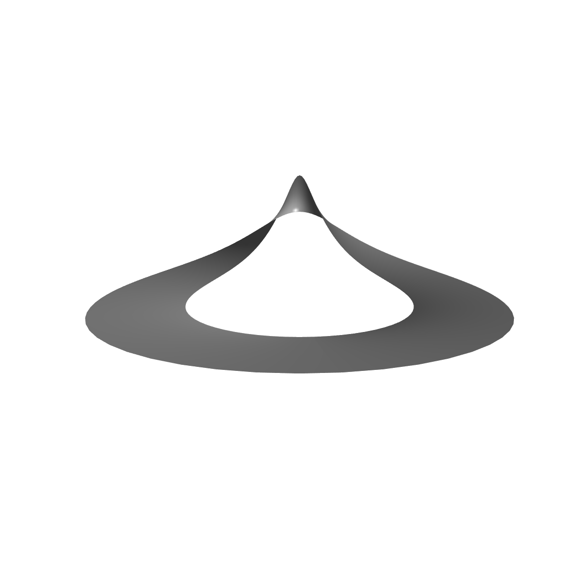
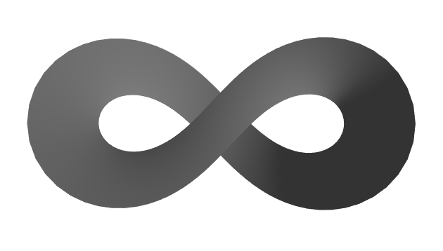
Figure 1. Two views of the same minimal cylinder in ${\rm Nil}_{3}$ from the hermitian potential $\zeta$ given in (3.1). The right-hand side picture is a rotation view of the left-hand side picture. The figures are made from MATLAB program of the loop group construction outlined in Appendix B programmed by David Brander (Technical University of Denmark).

Finally we point out that the minimal cylinder just constructed is not equivariant, since the Abresch-Rosenberg differential of the surface is $4(\cos^{2}z+\sin^{2}3z)dz^{2}$ which has zeros on $\mathbb{C}$ while it is constant on $\mathbb{C}$ for the equivariant case.

4. Homogeneous minimal surfaces in ${\rm Nil}_{3}$

The homogeneous minimal surfaces in ${\rm Nil}_{3}$ were classified in Appendix B of [21]. For the sake of completeness we recall this result.

4.1. Classification of homogeneous minimal surfaces

A surface $f:M\to{\rm Nil}_{3}$ is called homogeneous if there exists an injectively immersed Lie group $G\subset\operatorname{Iso}_{\circ}({\rm Nil}_{3})$ which acts transitively on $f(M)$.

Since $\operatorname{Iso}_{\circ}({\rm Nil}_{3})$ acts transitively on all of ${\rm Nil}_{3}$, clearly $G\neq\operatorname{Iso}_{\circ}({\rm Nil}_{3})$. If $\dim G=3$, then, for every point in $f(M)$, there exists a $1$-dimensional isotropy group. After left translation by same element in ${\rm Nil}_{3}\subset\operatorname{Iso}_{\circ}({\rm Nil}_{3})$, we can assume that $f(M)$ contains some element $c$ of the center of ${\rm Nil}_{3}$ and we take this element as our base point. Since ${\rm Nil}_{3}$ is normal in $\operatorname{Iso}_{\circ}({\rm Nil}_{3})$ one can write every $h\in\operatorname{Iso}({\rm Nil}_{3})$ in the form $h=p\phi$ where $p\in{\rm Nil}_{3}$ and $\phi\in\mathrm{U}_{1}$ as we have used in the proof of Theorem 1.5. We obtain $c=h(c)=pc$, whence $p=\mathrm{id}$. This shows that the isotropy group is ${\rm U}_{1}$ and we can assume without loss of generality that $G$ contains a $2$-dimensional subgroup $G_{0}\subset{\rm Nil}_{3}$ which already acts transitively. A simple argument with Lie algebras shows that there is, up to conjugacy, exactly one $2$-dimensional subgroup permitting conjugacy by elements of $\operatorname{Iso}_{\circ}({\rm Nil}_{3})$.

Finally, assume that we have some $2$-dimensional subgroup $G\subset\operatorname{Iso}_{\circ}({\rm Nil}_{3})$ which acts transitively on some minimal surface $f(\mathcal{R})$ in ${\rm Nil}_{3}$. We can assume again that $f(\mathcal{R})$ in ${\rm Nil}_{3}$ contains an element $c\in{\rm center(Nil_{3})}$ and that $G$ is not contained in ${\rm Nil}_{3}$.

Proposition 4.1.

Homogeneous surfaces in ${\rm Nil}_{3}$ are congruent to one of the following surfaces$:$

1. An orbit of a normal subgroup

   $$G(t)=\{(x_{1},tx_{1},x_{3})\in{\rm Nil}_{3}\ |\;x_{1},x_{3}\in\mathbb{R}\}\subset{\rm Nil}_{3},$$

   or

   $$G(\infty)=\{(0,x_{2},x_{3})\in{\rm Nil}_{3}\ |\;x_{2},x_{3}\in\mathbb{R}\}\subset{\rm Nil}_{3}.$$

2. An orbit of the Lie subgroup

   $$\{((0,0,s),e^{it})\ |\ s,t\in\mathbb{R}\}\subset{\rm Nil}_{3}\rtimes\mathrm{U}_{1}.$$

In the former case, surfaces are vertical planes. Surfaces in the latter case are Hopf cylinders over circles. Thus the only homogeneous minimal surfaces in ${\rm Nil}_{3}$ are vertical planes. In particular the quadratic differential $B$ vanishes identically on homogeneous surfaces.

Remark 4.2.

1. Note that part $(1)$ follows from [21] and part $(2)$ follows from Theorem 5.3 below.

2. The homogeneous minimal surfaces in ${\rm Nil}_{3}$ are exactly those minimal surfaces in ${\rm Nil}_{3}$ for which the function $w$ in (A.7) cannot be defined, that is, they are exactly those minimal surfaces in ${\rm Nil}_{3}$ for which the loop group approach does not work, that is, the case of $B\equiv 0$.

5. Equivariant minimal surfaces in ${\rm Nil}_{3}$

In this section we will discuss minimal surfaces in ${\rm Nil}_{3}$ which possess a one-parameter group of symmetries. We begin by stating the following basic definition.

Definition 5.1.

Let $f:\mathcal{R}\rightarrow{\rm Nil}_{3}$ be a surface. Then $f$ is called equivariant, if there exists a pair of one-parameter groups $(\gamma_{t},\rho_{t})\in\operatorname{Aut}(\mathcal{R})\times\operatorname{Iso}_{\circ}({\rm Nil}_{3})$ such that

(5.1) $$f\circ\gamma_{t}=\rho_{t}\circ f$$

holds.

In Theorem 5.9, we will show that if a minimal surface $S\subset{\rm Nil}_{3}$ is invariant under a one-parameter group $\rho_{t}\in\operatorname{Iso}_{\circ}({\rm Nil}_{3})$, $\rho_{t}.S=S$, there exists a special Riemann surface $\mathbb{S}$, an immersion $f:\mathbb{S}\to{\rm Nil}_{3}$ with $f(\mathbb{S})=S$ and a one-parameter group $\gamma_{t}\in\operatorname{Aut}(\mathbb{S})$ such that $f$ is equivariant in the sense of (5.1) with respect to $(\gamma_{t},\rho_{t})$.

5.1. One-parameter groups of $\operatorname{Iso}_{\circ}({\rm Nil}_{3})$

To carry out our study of equivariant minimal surfaces we will need a more detailed description of the isometry group $\operatorname{Iso}_{\circ}({\rm Nil}_{3})$. By definition, each element of the isometry group $\operatorname{Iso}_{\circ}({\rm Nil}_{3})={\rm Nil}_{3}\rtimes{\rm U}_{1}$ is of the form $((a_{1},a_{2},a_{3}),e^{i\theta})$. Recall the group multiplication

$$(a_{1},a_{2},a_{3})\cdot(x_{1},x_{2},x_{3})=\left(a_{1}+x_{1},a_{2}+x_{2},a_{3}+x_{3}+\frac{1}{2}(a_{1}x_{2}-a_{2}x_{1})\right)$$

of ${\rm Nil}_{3}$ and the action of $\operatorname{Iso}_{\circ}({\rm Nil}_{3})$ on ${\rm Nil}_{3}$:

$$((a_{1},a_{2},a_{3}),e^{i\theta})\cdot(x_{1},x_{2},x_{3})=(a_{1},a_{2},a_{3})\cdot(\cos\theta{x}_{1}-\sin\theta{x}_{2},\sin\theta{x}_{1}+\cos\theta{x}_{2},x_{3}).$$

Note, the isometry $((0,0,0),e^{i\theta})$ acts on ${\rm Nil}_{3}$ as a homomorphism of groups. It will be convenient to introduce a “shorthand writing” for certain typical group elements. We will use

$$\alpha\equiv((a_{1},a_{2},0),1),\quad\mathfrak{c}\equiv((0,0,\mathfrak{c}),1),\quad e^{i\theta}\equiv((0,0,0),e^{i\theta}).$$

Then everything is expressed in terms of $\alpha=(a_{1},a_{2})=a_{1}+ia_{2},\mathfrak{c}$ and $e^{i\theta}$. In particular we have: Each element $\rho$ of $\operatorname{Iso}_{\circ}({\rm Nil}_{3})$ can be written uniquely in the form

$$\rho=\alpha\mathfrak{c}e^{i\theta}.$$

Here is the list of the multiplications of the basic generators with respect to the semi-direct product group structure introduced above:

1. The group of all $\mathfrak{c}$ is a one-dimensional group isomorphic to $\mathbb{R}$.

2. The group of all ${e^{i\theta}}$ is a one-dimensional group isomorphic to $\mathbb{S}^{1}$.

3. The centralizer of $\operatorname{Iso}_{\circ}({\rm Nil}_{3})$ consist exactly of all $\mathfrak{c}$.

4. For $\alpha,\beta\in\mathbb{C}\cong\mathbb{R}^{2}$, $\alpha\beta=(\alpha+\beta)\mathfrak{c}(\alpha,\beta)$ holds, where $\mathfrak{c}(\alpha,\beta)=\frac{1}{2}\operatorname{Im}(\bar{\alpha}\cdot\beta)$ and “$\;\cdot\;$” denotes the multiplication of the complex numbers $\bar{\alpha}$ and $\beta$.

5. For $\beta\in\mathbb{C}\cong\mathbb{R}^{2}$, $e^{i\theta}\beta=(e^{i\theta}\cdot\beta)e^{i\theta}$, where “$\;\cdot\;$” again denotes the multiplication of the complex numbers $\beta$ and $e^{i\theta}$.

Putting this all together, one can easily verify

$$(\alpha\mathfrak{c}e^{i\theta})(\beta\mathfrak{d}e^{i\tau})=(\alpha+e^{i\theta}\cdot\beta)\left(\mathfrak{c}+\mathfrak{d}+\frac{1}{2}\operatorname{Im}(\bar{\alpha}\cdot e^{i\theta}\cdot\beta)\right)e^{i(\theta+\tau)}.$$

Note that the identity element in $\operatorname{Iso}_{\circ}({\rm Nil}_{3})$ is $1=((0,0,0),1)$ and

(5.2) $$(\alpha\mathfrak{c}e^{i\theta})^{-1}=e^{-i\theta}(-\mathfrak{c})(-\alpha)=(-e^{-i\theta}\cdot\alpha)(-\mathfrak{c})e^{-i\theta}.$$

Finally for $a=\alpha\mathfrak{c}\in{\rm Nil}_{3}$, we have $e^{i\theta}a=(e^{i\theta}\cdot\alpha)\mathfrak{c}e^{i\theta}$ and denotes it by

(5.3) $$e^{i\theta}a=e^{i\theta}[a]e^{i\theta},$$

that is, $e^{i\theta}[a]=(e^{i\theta}\cdot\alpha)\mathfrak{c}$. In particular $e^{i\theta}[\mathfrak{c}]=\mathfrak{c}$ follows. Finally we mention that the one-parameter group $\rho_{\theta}\in\operatorname{Iso}_{\circ}({\rm Nil}_{3})$ generated by the Killing vector field $E_{4}=-x_{2}\frac{\partial}{\partial x_{1}}+x_{1}\frac{\partial}{\partial x_{2}}$ consists of rotations $\rho_{\theta}=((0,0,0),e^{i\theta})$ of angle $\theta$ about the $x_{3}$-axis. In our shorthand writing this is $\rho_{\theta}=e^{i\theta}$.

An isometry $\rho^{(\mathfrak{c})}_{t}\in\mathrm{Nil}_{3}\rtimes\mathrm{U}_{1}$ of the form

$$\rho_{t}^{(\mathfrak{c})}=(\mathfrak{c}t)e^{it}=((0,0,\mathfrak{c}t),e^{it}),$$

where $\mathfrak{c}\in{\rm center(Nil_{3})},t\in\mathbb{R}$, is called a helicoidal motion with pitch $\mathfrak{c}$. By what was said above it is clear that this motion moves the points in ${\rm Nil}_{3}$ along the $e_{3}$-axis $\mathbb{R}e_{3}$ and rotates them about this axis simultaneously. The family of all transformations $\rho^{(\mathfrak{c})}_{t}$ forms for fixed $\mathfrak{c}$ a one-parameter group. In general, a helicoidal motion along the axis $\alpha+\mathbb{R}e_{3}$ through the point $\alpha=(a_{1}+ia_{2},0)=(a_{1},a_{2},0)\in\mathbb{R}^{2}\subset{\rm Nil}_{3}$ and with pitch $\mathfrak{c}$ has the form:

(5.4) $$\rho_{t}^{(\mathfrak{c},\alpha)}=\alpha\{(t\mathfrak{c})e^{it}\}\alpha^{-1}=(t\mathfrak{c})\{\alpha e^{it}\}\alpha^{-1}\in\operatorname{Iso}_{\circ}({\rm Nil}_{3}).$$

Clearly, the transformations $\rho_{t}^{(\mathfrak{c},\alpha)}\;(t\in\mathbb{R})$ form a one-parameter group. Moreover, a simple computation yields the natural and unique representation:

(5.5) $$\rho_{t}^{(\mathfrak{c},\alpha)}=(\alpha\cdot(1-e^{it}))\left(\mathfrak{c}t-\frac{|\alpha|^{2}}{2}\sin t\right)e^{it}.$$

A translation motion $\rho_{t}\in{\rm Nil}_{3}$ in direction $(a_{1},a_{2},\mathfrak{c})\in{\rm Nil}_{3}$ is given by

(5.6) $$\rho_{t}=(t\alpha)(t\mathfrak{c})\in\operatorname{Iso}_{\circ}({\rm Nil}_{3}).$$

In general one can consider any one-parameter group, not only a translation motion nor only a helicoidal motion along the axes $\alpha+\mathbb{R}e_{3},\alpha=a^{h}$. However, the following Theorem 5.3 implies that actually any one-parameter group which is not given by translations can be interpreted as a helicoidal motion, (for example [32, Theorem 2]).

Lemma 5.2.

Let $\rho=p\phi\in\operatorname{Iso}_{\circ}({\rm Nil}_{3})$ with $p=\pi_{0}\mathfrak{p}_{c}$, where $\pi_{0}\in\mathbb{R}^{2}$, $\mathfrak{p}_{c}\in{\rm center(Nil_{3})}$ and $\phi=e^{iq}\in{\rm U}_{1}$ for some $q\notin 2\pi\mathbb{Z}$. Then $\rho$ can be represented uniquely in the form

$$\rho=\mathfrak{c}\alpha\phi\alpha^{-1}$$

for some $\alpha\in\mathbb{R}^{2}\subset{\rm Nil}_{3}$ and $\mathfrak{c}\in{\rm center(Nil_{3})}$.

Proof.

We compute the coefficients of any expression of the form

$$\mathfrak{c}\alpha\phi\alpha^{-1}$$

with $\mathfrak{c}\in{\rm center(Nil_{3})}$, $\alpha=a^{h}=a_{1}+ia_{2}$ and $\phi=e^{iq}$. Since $\phi$ satisfies (5.3), $\phi\alpha=\phi[\alpha]\phi$ and we derive

$$\alpha\phi\alpha^{-1}=\alpha\left(\phi\alpha^{-1}\phi^{-1}\right)\phi=\alpha\phi[\alpha^{-1}]\phi.$$

Now a straightforward computation shows that $w=(\mathfrak{c}\alpha\phi\alpha^{-1})\phi$ has the coefficients

$$w_{1} =a_{1}-a_{1}\cos q+a_{2}\sin q,\quad w_{2}=a_{2}-a_{1}\sin q-a_{2}\cos q,\quad w_{3} =\mathfrak{c}-\frac{1}{2}(a_{1}^{2}+a_{2}^{2})\sin q,$$

where we set $w=(w_{1},w_{2},w_{3})\in{\rm Nil}_{3}$. Using $q\notin 2\pi\mathbb{Z}$ it is easy to prove that $(a_{1},a_{2},\mathfrak{c})\rightarrow(w_{1},w_{2},w_{3})$ is a diffeomorphism from $\mathbb{R}^{3}$ to $\mathbb{R}^{3}$. Therefore the $p$ defined by $\rho$ can be derived from some $(a_{1},a_{2},\mathfrak{c})$ and the claim follows. ∎

Theorem 5.3.

Assume $\rho_{t}$ is a one-parameter group in $\operatorname{Iso}_{\circ}({\rm Nil}_{3})$ which is not contained entirely in ${\rm Nil}_{3}$. Then with the notation of Lemma 5.2, $\rho_{t}$ can be represented in the form

$$\rho_{t}=\mathfrak{c}_{t}\alpha\phi_{t}\alpha^{-1},$$

where $\mathfrak{c}_{t}=t\mathfrak{c}\in{\rm center(Nil_{3})},\alpha=a^{h}\in{\rm Nil}_{3}$ is independent of $t$, and $\phi_{t}=e^{itq}$ with $q\neq 0$.

Proof.

Let $\rho_{t}$ denote the given one-parameter group. We can write $\rho_{t}=\pi_{t}\mathfrak{p}_{t}\phi_{t}$. Assuming without loss of generality $q(0)=0$ this decomposition is unique. By definition $\rho_{t+s}=\pi_{t+s}\mathfrak{p}_{t+s}\phi_{t+s}.$ Moreover,

$$\rho_{t}\rho_{s}=\pi_{t}\mathfrak{p}_{t}\phi_{t}\pi_{s}\mathfrak{p}_{s}\phi_{s}=\gamma_{t,s}\mathfrak{h}_{t,s}\phi_{t}\phi_{s}.$$

The equality $\rho_{t+s}=\rho_{t}\rho_{s}$ now implies that $\phi_{t}$ is a one-parameter group. Hence $\phi_{t}=e^{itq}$ where $q\neq 0$, otherwise $\rho_{t}$ would be contained entirely in ${\rm Nil}_{3}$. Now we write $\rho_{t}=\mathfrak{c}_{t}\alpha_{t}\phi_{t}\alpha_{t}^{-1}$ as in Lemma 5.2. Then

$$\rho_{s}\rho_{r}=(\mathfrak{c}_{s}\alpha_{s}\phi_{s}\alpha_{s}^{-1})(\mathfrak{c}_{r}\alpha_{r}\phi_{r}\alpha_{r}^{-1})=\rho_{r+s}.$$

Using formula $\phi a=\phi[a]\phi$ by (5.3), we rephrase the middle term above as

$$(\mathfrak{c}_{s}\alpha_{s}\phi_{s}\alpha_{s}^{-1})(\mathfrak{c}_{r}\alpha_{r}\phi_{r}\alpha_{r}^{-1}) =(\mathfrak{c}_{s}\alpha_{s}\phi_{s}[\alpha_{s}^{-1}])(\mathfrak{c}_{r}\phi_{s}[\alpha_{r}\phi_{r}[\alpha_{r}^{-1}]]\phi_{s+r})$$

$$=(\mathfrak{c}_{s}\mathfrak{c}_{r}\alpha_{s}\phi_{s}[\alpha_{s}^{-1}])(\phi_{s}[\alpha_{r}\phi_{r}[\alpha_{r}^{-1}]]\phi_{r+s}),$$

where we have also used that $\phi_{s}[\mathfrak{c}_{r}]=\mathfrak{c}_{r}$ holds, since $\phi[\mathfrak{c}]=\mathfrak{c}$ for all $\mathfrak{c}\in{\rm center(Nil_{3})}$. Comparing this to $\rho_{r+s}$ we observe

(5.7) $$(\mathfrak{c}_{r}\mathfrak{c}_{s}\alpha_{s}\phi_{s}[\alpha_{s}^{-1}])(\phi_{s}[\alpha_{r}\phi_{r}[\alpha_{r}^{-1}]])=\mathfrak{c}_{r+s}\alpha_{r+s}\phi_{r+s}[\alpha_{r+s}^{-1}].$$

Recall that $\alpha_{t}$ has no component in ${\rm center(Nil_{3})}$, that is, $\alpha_{t}=a_{t}^{h}$, whence $\phi_{t}[\alpha_{t}]=e^{iqt}\cdot\alpha_{t}$. But then $\alpha_{r+s}\phi_{r+s}[\alpha^{-1}_{r+s}]=\alpha_{r+s}-e^{iq(r+s)}\cdot\alpha_{r+s}$ modulo ${\rm center(Nil_{3})}$ and $(\alpha_{s}\phi_{s}[\alpha_{s}^{-1}])(\phi_{s}[\alpha_{r}\phi_{r}[\alpha_{r}^{-1}]])=\alpha_{s}-e^{isq}\cdot\alpha_{s}+e^{isq}\cdot(\alpha_{r}-e^{irq}\alpha_{r})$ modulo ${\rm center(Nil_{3})}$ follows. As a consequence we obtain the following equation of complex numbers

(5.8) $$(1-e^{iqs})\cdot\alpha_{s}+e^{iqs}\cdot(1-e^{iqr})\alpha_{r}=(1-e^{iq(r+s)})\cdot\alpha_{s+r}.$$

Differentiating (5.8) for $s$ at $s=0$ we obtain $-iq\cdot\alpha_{0}+iq(1-e^{iqr})\cdot\alpha_{r}=-iq\cdot e^{iqr}\cdot\alpha_{r}+(1-e^{iqr})\cdot\frac{d}{dr}\cdot\alpha_{r}$. This equation simplifies to yield

(5.9) $$iq\cdot(\alpha_{r}-\alpha_{0})=(1-e^{iqr})\cdot\frac{d}{dr}\alpha_{r}.$$

Differentiating (5.8) for $r$ at $r=0$, we obtain $e^{iqs}(-iq)\alpha_{0}=-iqe^{iqs}\cdot\alpha_{s}+(1-e^{iqs})\cdot\frac{d}{ds}\alpha_{s}$, which simplifies to

(5.10) $$iqe^{iqs}\cdot(\alpha_{s}-\alpha_{0})=(1-e^{iqs})\cdot\frac{d}{ds}\alpha_{s}.$$

From (5.9) and (5.10), we obtain that $\alpha_{t}$ is constant (say equal to $\alpha$). Since now $\alpha=\alpha_{r}=\alpha_{s}=\alpha_{r+s}$ and since also (5.7) holds, we obtain

(5.11) $$(\mathfrak{c}_{r}\mathfrak{c}_{s}\alpha\phi_{s}[\alpha^{-1}])(\phi_{s}[\alpha\phi_{r}[\alpha^{-1}]])=\mathfrak{c}_{r+s}\alpha\phi_{r+s}[\alpha^{-1}].$$

Since $\phi_{*}$ is a homomorphism of ${\rm Nil}_{3}$, we obtain

$$(\phi_{s}[\alpha^{-1}])(\phi_{s}[\alpha\phi_{r}[\alpha^{-1}]])=(\phi_{s}[\alpha^{-1}])(\phi_{s}[\alpha])(\phi_{s}[\phi_{r}[\alpha^{-1}]]).$$

Therefore the factors on the right cancel. This implies $\mathfrak{c}_{r}\mathfrak{c}_{s}=\mathfrak{c}_{r+s}$ and the claim follows. ∎

Remark 5.4.

The theorem above was stated (without proof) in Theorem 2 in [32].

In view of Theorem 5.3 above we introduce the following definition.

Definition 5.5.

Let $f:\mathcal{R}\to\mathrm{Nil}_{3}$ be a conformal immersion from a Riemann surface $\mathcal{R}$ into ${\rm Nil}_{3}$.

1. $f$ is said to be a helicoidal surface if the image $f(\mathcal{R})$ is invariant under a one-parameter group of helicoidal motions $\{\rho_{t}^{(\mathfrak{c},\alpha)}\}_{t\in\mathbb{R}}$ as defined in (5.5), that is,

   $$f(\mathcal{R})=\rho_{t}^{(\mathfrak{c},\alpha)}.f(\mathcal{R})$$

   holds for all $t\in\mathbb{R}$. In particular, $f$ is said to be a rotational surface if the helicoidal motion does not have a pitch.

2. $f$ is said to be a translation invariant surface if the image $f(\mathcal{R})$ is invariant under a one-parameter group of translation motions $\{\rho_{t}\}_{t\in\mathbb{R}}$ defined as in (5.6), that is,

   $$f(\mathcal{R})=\rho_{t}.f(\mathcal{R})$$

   holds for all $t\in\mathbb{R}$.

As a corollary of Theorem 5.3, we have the following.

Corollary 5.6.

The family of equivariant minimal surfaces in the sense of Definition 5.1 consists of all minimal helicoidal surfaces and all minimal translational surfaces.

Example 5.7.

The standard helicoid

$$f(x_{1},x_{2})=(x_{1},x_{2},\mathfrak{c}\tan^{-1}(x_{2}/x_{1}))$$

is a helicoidal minimal surface in $\mathrm{Nil}_{3}$. In fact this surface is invariant under the helicoidal motion of pitch $\mathfrak{c}$.

Remark 5.8.

Caddeo, Piu and Ratto [8] studied rotational surfaces of constant mean curvature (including minimal surfaces) in $\mathrm{Nil}_{3}$ via “equivariant submanifold geometry” in the sense of W. Y. Hsiang [36]. Moreover, Figueroa, Mercuri and Pedrosa [32] investigated surfaces of constant mean curvature invariant under some one-parameter isometry group. For minimal surfaces the results of this paper recover their results. The moduli space of all equivariant minimal surfaces in $\mathrm{Nil}_{3}$ will be given in the forthcoming paper [42].

5.2. Equivariance induced by one-parameter groups of $\operatorname{Iso}_{\circ}({\rm Nil}_{3})$

We now show that a one-parameter group of symmetries of a conformal minimal immersion $f$ from a Riemann surface $\mathcal{R}$ in ${\rm Nil}_{3}$ induces a minimal horizontal plane or a one-parameter group of symmetries for a conformal minimal immersion $\tilde{f}$ of a strip $\mathbb{S}$. More precisely we have the following theorem.

Theorem 5.9.

Let $f$ be a conformal minimal immersion from a Riemann surface $\mathcal{R}$ into ${\rm Nil}_{3}$ and $\rho_{t}$ a one-parameter group in $\operatorname{Iso}_{\circ}({\rm Nil}_{3})$ acting as a group of symmetries of $f$, that is, $\rho_{t}.f(\mathcal{R})=f(\mathcal{R})$ holds.

1. Assume that the one-parameter group $\rho_{t}$ acts with fixed points. Then $f(\mathcal{R})$ is a horizontal plane.

2. Assume that the one-parameter group $\rho_{t}$ acts without fixed points. Then there exists an open strip $\mathbb{S}\subset\mathbb{C}$ containing the real axis and an immersion $\tilde{f}:\mathbb{S}\to{\rm Nil}_{3}$ such that $f(\mathcal{R})=\tilde{f}(\mathbb{S})$ and

   $$\rho_{t}.\tilde{f}(z)=\tilde{f}(\gamma_{t}.z),$$

   for all $z\in\mathbb{S}$, holds.

Proof.

(1): Since $\rho_{t}$ is classified as in Definition 5.5 and has fixed points by assumption, it must be a rotation around the axis through a point $(a,b,0)\in{\rm Nil}_{3}$ parallel to the $e_{3}$-axis. Then we can choose a simply-connected domain $\tilde{\mathbb{D}}\subset\mathbb{C}$ which contains $z=0$ and a minimal immersion $\tilde{f}:\tilde{\mathbb{D}}\to{\rm Nil}_{3}$ such that $\tilde{f}(\tilde{\mathbb{D}})\subset f(\mathcal{R})$ and $\tilde{f}(0)$ is one of fixed points of $\rho_{t}$. Moreover there exists a $\gamma_{t}:z\mapsto ze^{it}$ as a local one-parameter group of $\tilde{\mathbb{D}}$ such that $0\in\tilde{\mathbb{D}}$ is a fixed point of $\gamma_{t}$ and $\tilde{f}$ is equivariant with respect to $(\gamma_{t},\rho_{t})$. Then for the harmonic normal Gauss map $g:\mathbb{D}\rightarrow\mathbb{H}^{2}$ and an extended frame $F$ of $f$ we obtain

(5.12) $$g(\gamma_{t}.z,\overline{\gamma_{t}.z})=e^{iat}g(z,\bar{z})$$

for some $a\in\mathbb{R}$ and the extended frame $F$ satisfies

(5.13) $$F(\gamma_{t}.z,\overline{\gamma_{t}.z},\lambda)=M_{t}(\lambda)F(z,\bar{z},\lambda)k(t,z,\bar{z}),$$

where $M_{t}(\lambda)\in\Lambda{\rm SU}_{1,1\sigma}$ and $M_{t}(\lambda=1)=\operatorname{diag}(e^{ait/2},e^{ait/2})$ and $k(t,z,\bar{z})\in{\rm U}_{1}$, see Proposition 2.1. For $z=0$ we infer

(5.14) $$F(0,\lambda)=M_{t}(\lambda)F(0,\lambda)k(t,0),$$

Replacing $F$ by $\hat{F}(z,\bar{z},\lambda)=F(0,\lambda)^{-1}F(z,\bar{z},\lambda)$, we obtain $\hat{F}(0,\lambda)=\operatorname{id}$ and, setting $\hat{M}_{t}(\lambda)=F(0,\lambda)^{-1}M_{t}(\lambda)F(0,\lambda)$ we derive

(5.15) $$\hat{F}(\gamma_{t}.z,\overline{\gamma_{t}.z},\lambda)=\hat{M}_{t}(\lambda)\hat{F}(z,\bar{z},\lambda)k(t,z,\bar{z}).$$

As a consequence we obtain

(5.16) $$\hat{M}_{t}(\lambda)=k(t,0)^{-1}=k_{0}(t).$$

In particular, $k_{0}(t)=\hat{M}_{t}(\lambda)$ is independent of $\lambda$ and contained in ${\rm U}_{1}$. Hence $\hat{M}_{t}(\lambda)$ is diagonal. As a consequence we have two cases:

Case 1. $\hat{M}_{t}(\lambda)=\operatorname{id}$ for all $t\in\mathbb{R}$. In this case also $M_{t}(\lambda)=\operatorname{id}$ for all $t\in\mathbb{R}$. But then $f(e^{it}z)=f(z)$ for all $t\in\mathbb{R}$ and $f$ is not a surface.

Case 2. $\hat{M}_{t}(\lambda)=k_{0}(t)=\operatorname{diag}(e^{iat/2},e^{iat/2})\neq\operatorname{id}$, that is, $a\in\mathbb{R}\setminus 2\pi\mathbb{Z}$. Since $\hat{F}(0,\lambda)=\operatorname{id}$ we can perform the Birkhoff decomposition $\hat{F}(z,\bar{z},\lambda)=\hat{F}_{-}(z,\lambda)\hat{L}_{+}(z,\bar{z},\lambda)$ around $z=0$ and obtain

(5.17) $$\hat{F}_{-}(\gamma_{t}.z,\lambda)=k_{0}(t)\hat{F}_{-}(z,\lambda)k_{0}(t)^{-1}.$$

Note that $\hat{F}(0,0,\lambda)=\operatorname{id}$ implies that $\hat{F}_{-}$ is holomorphic with respect to $z$ in an open neighbourhood of $z=0$. Let $\eta_{-}(z,\lambda)=\hat{F}_{-}^{-1}d\hat{F}_{-}$, then $\eta_{-}(z,\lambda)=\lambda^{-1}\xi(z)dz$ is the normalized potential associated with the minimal surface $f$, the normal Gauss map $g$, and the frame $\hat{F}$. Then we obtain from (5.17):

(5.18) $$\xi(e^{it}z)e^{it}=k_{0}(t)\xi(z)k_{0}(t)^{-1}.$$

Writing

(5.19) $$\xi=\lambda^{-1}\begin{pmatrix}0&-p\\ Bp^{-1}&0\end{pmatrix},$$

the equation (5.18) yields

(5.20) $$p(e^{it}z)e^{it}=e^{iat}p(z),$$

and we have

(5.21) $$B(e^{it}z)e^{2it}=B(z),$$

since $B(z)dz^{2}$ is a globally defined quadratic differential. Note that $a$ takes values in $\mathbb{R}\setminus 2\pi\mathbb{Z}$. From the last equation it now follows that $B(z)$ is identically zero.

From equation (5.20) we infer that $p$ is of the form $p(z)=p_{j}z^{j}$ for some $j\in\mathbb{Z}$ and $p_{j}\neq 0$. Moreover, $j+1=a$ holds.

Since we know that $\hat{F}_{-}$ is holomorphic at $z=0$ it follows that $p$ is holomorphic at $z=0$, whence $j\geq 0$ follows. Now, if $j>0$, then the surface $f$ has a branch point at $z=0$, a contradiction. As a consequence, $j=0$. This case has already been considered in [21, Section 6] and it was shown that the corresponding minimal surfaces are horizontal planes. Then since the Abresch-Rosenberg differential $Bdz^{2}$ vanishes on $\tilde{f}(\tilde{\mathbb{D}})\subset f(\mathcal{R})$, it vanishes on $f(\mathcal{R})$ and the whole surface $f(\mathcal{R})$ is the horizontal plane.

(2): Since $\rho_{t}$ acts without fixed points on $f(\mathcal{R})$, around any $p_{0}\in f(\mathcal{R})$ there exists a chart $\psi_{0}:\mathbb{D}_{0}\rightarrow{\rm Nil}_{3}$ such that $\psi(0)=p_{0}$ and $\mathbb{D}_{0}$ is an open rectangle containing the origin and with axes parallel to the usual coordinate axes of $\mathbb{R}^{2}$. Moreover, for all $z\in\mathbb{D}_{0}$ and sufficiently small $t\in I=(-\epsilon,\epsilon)$ we have with $f_{0}=f\circ\psi_{0}$:

$$f_{0}(z+t)=\rho_{t}.f_{0}(z).$$

This follows from the fact that the (never vanishing) vector field generating the one-parameter group action $\rho_{t}$ can be represented as $\frac{\partial}{\partial x}$ in some chart.

Let $\mathbb{S}$ denote the strip parallel to the real axis and containing $\mathbb{R}$ which has the same height as $\mathbb{D}_{0}$. By [7] there exists a Delaunay type matrix $D(\lambda)$ which generates a minimal immersion $f_{o}^{\sharp}$ on $\mathbb{S}$ which coincides with $f_{0}$ on $\mathbb{D}_{0}$, see also Theorem 5.20.

We claim $f_{o}^{\sharp}(\mathbb{S})\subset f(\mathcal{R})$. Suppose this is wrong, then there exists a line segment $L$ in $\mathbb{S}$, parallel to the $x$-axis, such that $f_{o}^{\sharp}$ leaves $f(\mathcal{R})$ at some endpoint $l_{0}$ of $L$. Let us write $l_{0}=(t_{0},y_{0})$ and let us assume without loss of generality $t_{0}>0.$ Let $s>0$ such that $(s,y_{0})\in\mathbb{D}_{0}.$ Then $t_{0}=ms+s^{*}$ with $0<s^{*}<s$ and $m\in\mathbb{Z}$. As a consequence $f_{0}^{\sharp}(0+t_{0})=(\rho_{s})^{m}.f_{0}(s^{*})\in f(\mathcal{R})$. Now we can choose a small chart around $q_{0}=f_{0}^{\sharp}(t_{0})$ which corresponds to a small box in $\mathbb{R}^{2}$ centered at $(t_{0},y_{0})$ such that, analogous to the argument above, $f_{0}^{\sharp}$ maps the small box into $f(\mathcal{R})$. Hence $f_{0}^{\sharp}$ maps a strictly larger line segment $L\subset L^{\sharp}$ into $f(\mathcal{R})$. This contradiction implies $f_{0}^{\sharp}(\mathbb{S})\subset f(\mathcal{R})$.

Finally we want to show $f_{0}^{\sharp}(\mathbb{S})=f(\mathcal{R})$. For this we choose $\mathbb{S}$ considered above as large as possible. Let us consider first the case, where $\mathbb{S}$ ends in the upper half-plane at the line $T_{u}$ and in the lower half-plane at the line $T_{l}$, both parallel to the $x$-axis. If there exists any point in $f(\mathcal{R})$ which is not contained in $f_{0}^{\sharp}(\mathbb{S})$, then we choose a curve in $f(\mathcal{R})$ connecting such a point with $f_{0}^{\sharp}(0)$. This curve needs to intersect $f_{0}^{\sharp}(T_{u})$ or $f_{0}^{\sharp}(T_{l}).$ At a point of intersection we apply the argument above and obtain an open strip containing the corresponding boundary line of the image of $f_{0}^{\sharp}$. Therefore $f_{0}^{\sharp}$ can be extended beyond this boundary line, a contradiction. We thus only need to consider the case ,where the strip is either half-infinite or all of $\mathbb{C}$ and where in $f(\mathcal{R})$ there is a boundary point $q_{0}$ of $f_{0}^{\sharp}(\mathbb{S})$, which can be obtained by taking a limit to $\infty$ inside $\mathbb{S}$. Then by the argument above we obtain a finite open strip $\mathbb{B}$ containing $q_{0}$ and an equivariant conformal map $f_{0}^{\prime}$ such that on some sub-strip of $\mathbb{B}$ and some half-plane the conformal maps $f_{0}^{\sharp}$ and $f_{0}^{\prime}$ have the same image. Since both maps are equivariant under real translations, they induce a bi-holomorphic change of coordinates of the type $(x,y)\mapsto(x,h(y))$. Hence $h(y)=y+c$. This is impossible, since one strip has infinite width and the other one has only finite width. ∎

Remark 5.10.

Above we have shown that the invariance of $f(\mathcal{R})$ under a one-parameter group without fixed points can be realized by an immersion of some open strip $\mathbb{S}$. However, in general it is not possible to define a one-parameter group on the original surface $\mathcal{R}$.

5.3. One-parameter groups of $\operatorname{Aut}(\mathcal{R})$

It is well known that only a few Riemann surfaces admit a one-parameter group of automorphisms. For non-compact simply-connected Riemann surfaces only the following cases occur (up to conjugation by bi-holomorphic automorphisms (see, for example [28, Section V-4]): Let us denote the complex plane by $\mathbb{C}$ and the upper half plane by $\mathbb{H}$, that is $\mathbb{H}=\{z\in\mathbb{C}\;|\;\operatorname{Im}z>0\}$.

1. $\mathbb{C}$ and all translations parallel to the $x$-axis,

2. $\mathbb{C}$ and all multiplications $z\rightarrow e^{ta}z$ with $a\in\mathbb{C}^{*}$.
   

3. $\mathbb{H}$ and all translations parallel to the real axis,

4. $\mathbb{H}$ and all multiplications $z\rightarrow az$ with $a$ positive real,

5. $\mathbb{H}$ and all automorphisms fixing the point $i$.

In the cases (1b) and (2c) the Riemann surface contains a point which is fixed by the one-parameter group. We will show in Theorem 5.13 below that these cases only consist of very special minimal surfaces. In case (1b), if one removes the origin and considers the map $\mathbb{C}\rightarrow\mathbb{C}^{*}=\mathbb{C}\smallsetminus\{0\},w\rightarrow e^{aw}$, then the group action pulls back to translation parallel to the $x$-axis. A similar observation holds in case (2c), if one interprets it as rotation about the origin of the unit disk. In case (2b), one can map $\mathbb{H}$ via $z\rightarrow\log(z)-i\pi/2$ to the strip parallel to the real axis between $y=\pi/2$ and $y=-\pi/2$ such that the one-parameter group turns into the group of translations parallel to the real axis.

In the following cases one can consider the universal cover and thus obtains strips with the one-parameter group of translations parallel to the real axis.

1. $\mathbb{H}^{2}_{*}=\mathbb{H}^{2}\smallsetminus\{0\}$ and all rotations about the origin,

2. $\mathbb{C}^{*}$ and all multiplications $z\rightarrow e^{ta}z$ with $a\in\mathbb{C}^{*}$,

3. $\mathbb{A}_{a,b}$ and all rotations about the origin, where $0<a<b$ and $\mathbb{A}_{a,b}=\{z\in\mathbb{C},0<a<|z|<b\}$.

Beyond the cases listed above, only tori admit one-parameter groups of automorphisms. Note that above already all conformal types of cylinders have been listed.

Definition 5.11.

Equivariant surfaces for which the group acts by translations (on a strip) will be called $\mathbb{R}$-equivariant. Equivariant surfaces for which the group acts by rotations (about a point) will be called $\mathbb{S}^{1}$-equivariant.

The cases (1b) and (3b) do not fall directly into these two categories. Note, all $\mathbb{S}^{1}$-equivariant cases have a natural fixed point contained in the domain of definition, or not.

Theorem 5.12.

Let $f:\mathcal{R}\to{\rm Nil}_{3}$ be an equivariant minimal surface of the type (3a), (3b) or (3c). Since the fixed point of $\gamma_{t}$ is not contained in $\mathcal{R}$, one can realize the universal cover $\mathbb{S}$ of $\mathcal{R}$ as a strip containing the $x$-axis, such that the induced map $\tilde{f}:\mathbb{S}\rightarrow{\rm Nil}_{3}$ is $\mathbb{R}$-equivariant relative to all real translations in the first two cases and in direction $a$ in the last case. Moreover, in the cases (3a) and (3c) $\tilde{f}$ is periodic and has a $($smallest$)$ positive real period, and in the case (3b) the period is $2\pi/a$.

Proof.

We only need to prove the last assertion. Suppose there does not exist a smallest positive period. Then there exists a sequence $p_{n}$ of positive periods converging to $0$. Since $f$ is real analytic, $f$ is constant, a contradiction, since $f$ is assumed to be a surface. In the case (3b) we consider the universal cover $\pi_{a}:\mathbb{C}\rightarrow\mathbb{C}^{*},w\rightarrow e^{aw}$. Then the given action corresponds to $w\rightarrow w+t$. Hence the period is $2\pi/a$. ∎

5.4. Special equivariant minimal surfaces

Next we will show that $\mathbb{S}^{1}$-equivariant minimal surfaces with fixed point or vanishing Abresch-Rosenberg differential are very special.

Theorem 5.13.

1. Consider an equivariant minimal surface in ${\rm Nil}_{3}$ with fixed point in ${\rm Nil}_{3}$, that is, it is in one of the cases (1b) or (2c). Then the Abresch-Rosenberg differential vanishes identically and such a minimal surface is only a horizontal plane.

2. Consider an equivariant minimal surface in ${\rm Nil}_{3}$ without fixed point and vanishing Abresch-Rosenberg differential. Then such a minimal surface is only a vertical plane.

Proof.

(1) The statement follows directly from $(1)$ in Theorem 5.9.

(2) By Proposition 2 in [21], such a minimal surface is only a horizontal plane or a vertical plane. The only vertical plane does not have any fixed point. ∎

5.5. Basics about $\mathbb{R}$-equivariant minimal surfaces

By our discussion in Sections 5.3 and 5.4, from here on we only need to consider $\mathbb{R}$-equivariant surfaces which are defined on some strip $\mathbb{S}$ and have non-vanishing Abresch-Rosenberg differentials. Specific properties of the different cases will be discussed elsewhere. For simplicity of notation we will, as before, abbreviate a function $p(z,\bar{z})$ by $p(z)$. Hence the expression $p(z)$ does not necessarily denote a function depending only on $z$.

Theorem 5.14.

Let $f:\mathbb{S}\to{\rm Nil}_{3}$ be an $\mathbb{R}$-equivariant minimal surface relative to the one-parameter group $(\gamma_{t},\rho_{t})$, $\gamma_{t}.z=z+t$, and $\rho_{t}$ a one-parameter group in $\operatorname{Iso}_{\circ}({\rm Nil}_{3})$ which is not contained in ${\rm Nil}_{3}$. Let $g$ denote the $($non-holomorphic$)$ normal Gauss map of $f$. Then we obtain

(5.22) $$f(z+t)=\rho_{t}.f(z)\quad\mbox{and}\quad g(z+t)=e^{iat}g(z)$$

with $0\neq a\in\mathbb{R}$.

Moreover,

1. For an extended frame $F$ of $f$ as given in (A.17), there exists some $k(t,z)\in{\rm U}_{1}$ satisfying

   (5.23) $$F(z+t,\lambda)=M_{t}(\lambda)F(z,\lambda)k(t,z),$$

   where $M_{t}\in\Lambda{\rm SU}_{1,1\sigma}$, $M_{t}(\lambda=1)=\operatorname{diag}(e^{iat/2},e^{-iat/2}).$

2. There exists a unitary diagonal matrix $\ell$ such that the frame $F_{\ell}=F\ell$ satisfies $k_{\ell}(t,z)\equiv\operatorname{id}$.

Proof.

The transformation behaviour (5.23) of $F$ follows, since $F:\mathbb{S}\rightarrow\Lambda{\rm SU}_{1,1\sigma}$ is a lift of $g:\mathbb{S}\rightarrow\mathbb{H}^{2}$, see also (1.12). Also note, since $M_{t}|_{\lambda=1}$ is a homomorphism, it is easy to verify that $k(t,z)$ satisfies the cocycle condition

(5.24) $$k(t+s,z)=k(t,z)k(s,z+t),$$

and we obtain (see for example Theorem 2.2 and [25, Theorem 4.1]):

$$k(t,z)=\ell(z)\ell(z+t)^{-1},$$

where $\ell(z)=\ell(x+iy)=k(x,iy)^{-1}$. As a consequence, replacing the original frame $F$ by $F\ell$ one obtains an extended frame as desired. ∎

Remark 5.15.

1. In the theorem above one could also permit one-parameter families $\rho_{t}$ which are contained in ${\rm Nil}_{3}$. This case will be discussed in Section 5.10 below.

2. Theorem 5.14 also holds for any general extended frame $F$ of a harmonic map $g$ which satisfies (5.22).

Definition 5.16.

A general extended frame satisfying

$$F(z+t,\lambda)=M_{t}(\lambda)F(z,\lambda)$$

will be called $\mathbb{R}$-equivariant.

5.6. A chain of extended frames

For a detailed discussion of the relation between spacelike CMC surfaces in Minkowski $3$-space $\mathbb{L}^{3}$ and minimal surfaces in ${\rm Nil}_{3}$ it is important to use extended frames with specific additional properties. In [21], also see (A.17), a specific extended frame was defined for all $\lambda=1$ and the matrix entries were (by definition) the spinors associated with the associated family $\{f^{\lambda}\}_{\lambda\in\mathbb{S}^{1}}$ of $f$. Note that the spinors of a minimal surface in ${\rm Nil}_{3}$ are defined uniquely up to a common sign. By continuity in $\lambda$, the choice of sign for the $\psi_{j}$ thus is the same for all $\lambda$, whence irrelevant.

Hence the first extended frame in our chain is an extended frame mentioned above and denoted by $F(z,\lambda)$ in (5.23). As pointed out in Theorem 5.14, this extended frame will, in general, not be $\mathbb{R}$-equivariant under the action of the translational one-parameter group $z\rightarrow z+t$. But we have shown that there exists some function $\ell(z)$ such that $F_{\ell}=F\ell$ defines an $\mathbb{R}$-equivariant general extended frame for the translational one-parameter group. The frame $F_{\ell}$ is our second frame. Finally we consider an $\mathbb{R}$-equivariant extended frame which also attains the value $\operatorname{id}$ at $z=0$ for all $\lambda$: $\hat{F}(z,\lambda)=F_{\ell}(0,\lambda)^{-1}F_{\ell}(z,\lambda)$.

Thus we have the following triple of extended frames

(5.25) $$F\longrightarrow F_{\ell}\longrightarrow\hat{F}.$$

Remark 5.17.

Note, the frames $F$ and $F_{\ell}$ generate the same surfaces in $\mathbb{L}^{3}$ and in ${\rm Nil}_{3}$ via the respective Sym formulas. The frame $\hat{F}$ generates in $\mathbb{L}^{3}$ a surface which is isometric to the previously generated surface, but the corresponding surface in ${\rm Nil}_{3}$ has, in general, no simple relation to the other (two) surfaces in ${\rm Nil}_{3}$. However, as will explained below, exactly this frame yields a very simple “degree-one-potential” from which we will be able to construct what we want. Note, in such a chain, if one assumes that any of these extended frames has a translational one-parameter group of symmetries, then all three frames have such a symmetry. The frames $\hat{F}$ are $\mathbb{R}$-equivariant general extended frames of the normal Gauss map $g$, where $g:\mathbb{S}\rightarrow\mathbb{H}^{2}$ is non-holomorphic (since the surface has non-vanishing Abresch-Rosenberg differential) harmonic, and also define spacelike CMC surfaces in Minkowski 3-space $\mathbb{L}^{3}$. For more details on $\mathbb{R}$-equivariant harmonic maps see, for example [7] and for spacelike CMC surfaces in $\mathbb{L}^{3}$ see, for example [5].

5.7. The construction principle

In order to construct $\mathbb{R}$-equivariant minimal surfaces in ${\rm Nil}_{3}$ we will start in general from some special potential and will arrive at some $\mathbb{R}$-equivariant general extended frame $\hat{F}$, assuming the monodromy has the required properties. (In a sense just reversing the arrows in (5.25) above.) What special potentials we will need to start from will be the contents of the next sections.

At any rate, we will obtain the transformation behaviour (for $t\in\mathbb{R}$ and $z\in\mathbb{S}^{\prime}$):

$$\hat{F}(z+t,\lambda)=\hat{M}_{t}(\lambda)\hat{F}(z,\lambda)$$

and we also know $\hat{F}(0,\lambda)=\operatorname{id}$. We will apply [7] to construct all of such frames. Note, while the potential will be defined on some strip $\mathbb{S}$, $\hat{F}$ may be defined on some smaller strip $\mathbb{S}^{\prime}$ only, see [42].

After $\hat{F}$ has been constructed we want to use this frame to construct $\mathbb{R}$-equivariant minimal surfaces in ${\rm Nil}_{3}$. But for this it is important to require that $\hat{M}_{t}$ is diagonalizable for $\lambda=1.$ In particular, the eigenvalues of $\hat{M}_{t}$ need to be unimodular at $\lambda=1$, see Theorem 5.14. Therefore, in general, we need to change the frame $\hat{F}$ to another frame, for which the monodromy is diagonal for $\lambda=1$. This is achieved by putting $F=SF$, where $S$ diagonalizes the monodromy as required. (For more details see below.) Comparing to the chain of frames above we observe, that this new frame plays the role of $F_{\ell}$.

Remark 5.18.

The general extended frame $\hat{F}$ with the right choice of initial condition $S$ gives the extended frame $F_{\ell}=S\hat{F}$, which is not $F$. However, this is irrelevant for the resulting minimal immersion $f$. More precisely, if one plugs $F$ and $F_{\ell}$ into the Sym formula, then the resulting minimal surfaces are the same. Thus we will only consider $F_{\ell}$.

As pointed out already above, the change from $\hat{F}$ to $F_{\ell}$ is by multiplication:

$$F_{\ell}(z,\lambda)=S(\lambda)\hat{F}(z,\lambda)$$

with $S(\lambda)\in\Lambda{\rm SU}_{1,1\sigma}$. Note since $\hat{M}_{t}$ is diagonalizable at $\lambda=1$ for all $t\in\mathbb{R}$, one can choose $S(\lambda)$ such that the monodromy $M_{t}(\lambda)=S(\lambda)\hat{M}_{t}(\lambda)S(\lambda)^{-1}$ of $F_{\ell}$ is diagonal for $\lambda=1$. More precisely, since $\hat{M}_{t}(\lambda=1)$ diagonalizable, we have two cases:

Case 1. The eigenvalues of $\hat{M}_{t}(\lambda=1)$ are both $1$. This means $\hat{M}_{t}(\lambda=1)=\operatorname{id}$. Then we can choose $S(\lambda)\in\Lambda{\rm SU}_{1,1\sigma}$ arbitrary.
Case 2. The unimodular eigenvalues of $\hat{M}_{t}(\lambda=1)$ are different. In this case there exists some matrix $S\in{\rm SU}_{1,1}$ such that $S\hat{M}_{t}(\lambda=1)S^{-1}$ is diagonal. Inserting $\lambda$ and $\lambda^{-1}$ respectively off-diagonal into $S$ we obtain a matrix $S(\lambda)\in\Lambda{\rm SU}_{1,1\sigma}$ such that $M_{t}(\lambda)=S(\lambda)\hat{M}_{t}(\lambda)S(\lambda)^{-1}$ is diagonal for $\lambda=1$.

Altogether we obtain that $F_{\ell}(z,\lambda)=S(\lambda)\hat{F}(z,\lambda)$ is a general extended frame for $g$ which has monodromy $M_{t}(\lambda)$, and $M_{t}(\lambda=1)$ is diagonal. As a consequence, we obtain an $\mathbb{R}$-equivariant minimal surface in ${\rm Nil}_{3}$ defined on some strip $\mathbb{S}^{\prime}$ containing the real axis by applying the Sym formula stated in Section C.2.

Remark 5.19.

In both cases above the choice of “initial condition” $S\in\Lambda{\rm SU}_{1,1\sigma}$ is not unique. Here is what happens for different choices:

Case 1. In the case of $\hat{M}_{t}(\lambda=1)=\operatorname{id}$ different initial conditions generally yield different equivariant minimal surfaces, see Section 5.10.

Case 2. Assume the eigenvalues of $\hat{M}_{t}(\lambda=1)$ are unimodular and different. Let $\tilde{S}\in\Lambda{\rm SU}_{1,1\sigma}$ be another initial condition such that $\tilde{S}\hat{M}_{t}\tilde{S}|_{\lambda=1}=S\hat{M}_{t}S^{-1}|_{\lambda=1}$. Then $\tilde{S}=\delta S$ with some loop $\delta\in\Lambda{\rm SU}_{1,1\sigma}$ such that $\delta|_{\lambda=1}$ is diagonal. Let $F_{\ell}$ and $\tilde{F}_{\ell}$ be the corresponding general extended frames associated with the initial conditions $S$ and $\tilde{S}$, respectively. Then we obtain $\tilde{F}_{\ell}=\delta F_{\ell}$. Inserting $F_{\ell}$ and $\tilde{F}_{\ell}$ into the Sym formula, the resulting minimal surfaces are the same up to a rigid motion (see the proof of (b) of Theorem 1.5 for the computation).

5.8. Degree one potentials

In the last subsection we have seen that for every $\mathbb{R}$-equivariant minimal surface in ${\rm Nil}_{3}$ its normal Gauss map is an $\mathbb{R}$-equivariant harmonic map into $\mathbb{H}^{2}$. These maps have been investigated in [5]. It will be more helpful to us to follow the approach of [7], translated into our setting. Here is our rendering of results of these two papers which are particularly relevant to this paper.

We consider $f:\mathbb{S}\to{\rm Nil}_{3}$ to be an $\mathbb{R}$-equivariant minimal surface relative to the one-parameter group $(\gamma_{t},\rho_{t})$, $\gamma_{t}.z=z+t$, that is,

$$f(\gamma_{t}.z)=\rho_{t}.f(z).$$

Let $g:\mathbb{S}\rightarrow\mathbb{H}^{2}$ denote its (non-holomorphic) harmonic normal Gauss map and $\hat{F}$ an $\mathbb{R}$-equivariant general extended frame for $g$ which attains the value identity at $0$. Let $\hat{M}_{t}(\lambda)\in\Lambda{\rm SU}_{1,1\sigma}$ denote the monodromy of $\hat{F}$.

By following [7, Section 3] in our setting and [5] we obtain the following characterization of all $\mathbb{R}$-equivariant minimal surfaces in ${\rm Nil}_{3}$:

Theorem 5.20.

Every $\mathbb{R}$-equivariant non-holomorphic harmonic map $g:\mathbb{S}\rightarrow\mathbb{H}^{2}$ associated with an $\mathbb{R}$-equivariant minimal surface in ${\rm Nil}_{3}$ can be obtained from a constant holomorphic potential $\eta=Ddz$ of the form

(5.26) $$D\in\Lambda\mathfrak{su}_{1,1\sigma},\quad D(\lambda)=\lambda^{-1}w_{-1}+w_{0}+\lambda w_{1},\quad\det D(\lambda=1)\geq 0,\quad(w_{-1})_{12}\neq 0,$$

where all $w_{j}$ are independent of $\lambda$ and $z$ and $(w_{-1})_{12}$ denotes the $(1,2)$-entry of $w_{-1}$. In particular $D$ has purely imaginary eigenvalues for $\lambda=1$.

Conversely, every constant $\eta=Ddz$ as in (5.26) with initial condition $S\in\Lambda{\rm SU}_{1,1\sigma}$ such that $SDS^{-1}|_{\lambda=1}$ is diagonal, generates an $\mathbb{R}$-equivariant harmonic map $g:\mathbb{S}\rightarrow\mathbb{H}^{2}$ defined on some strip $\mathbb{S}\subset\mathbb{C}$ parallel to the real axis, and, by the Sym-formula (C.3), generates an $\mathbb{R}$-equivariant minimal surface in ${\rm Nil}_{3}.$

Proof.

Following the proof of [7, Section 3] verbatim we obtain the first two statements of (5.26). The last statement expresses the fact that we assume $f$ to be an immersion at the base point “$z=0$”. Hence, to finish the proof of the first part of the claim we only need to prove the statement about the eigenvalues of $D$. But for the monodromy $\hat{M}_{t}$ of $\hat{F}$ defined in the last subsection we have $\hat{M}_{t}(\lambda)=F_{\ell}(0,\lambda)^{-1}M_{t}(\lambda)F_{\ell}(0,\lambda)$. Thus $\hat{M}_{t}(\lambda=1)$ has the same eigenvalues as $M_{t}(\lambda=1)$, where $M_{t}$ is the monodromy of a general extended frame $F_{\ell}$. But $\hat{M}_{t}(\lambda)=\exp(tD(\lambda))$ by definition of $D(\lambda$), see [7], and we know that $\hat{M}_{t}(\lambda=1)$ is diagonalizable for all $t$. Hence $D(\lambda=1)$ has only purely imaginary eigenvalues and the claim follows. The proof of the second part of the claim follows from [7, Section 3] and the fact that we need diagonalizable monodromy in our situation. ∎

Remark 5.21.

1. The potential $\eta=Ddz$ will be called the degree one potential of an $\mathbb{R}$-equivariant minimal surface $f$.

2. The theorem above does not specify the size of the strip $\mathbb{S}$ in the second part of the theorem, since the Iwasawa decomposition of $\exp(zD)$ is not global. This issue will be discussed in the forthcoming paper [42].

3. Since $D\in\Lambda\mathfrak{su}_{1,1\sigma}$, the diagonalizablity condition in Theorem 5.20 immediately implies that $\det D(\lambda=1)\geq 0$ and moreover, when $\det D(\lambda=1)=0$, then $D(\lambda=1)=0$ follows. On the contrary, in Proposition 5.31 when $\det D(\lambda=1)=0$ and $D(\lambda=1)\neq 0$ or $\det D(\lambda=1)<0$, we obtain non-equivariant minimal immersions which have an equivariant normal Gauss map.

With the notation of Theorem 5.20, and the explanation of the construction principle in the previous subsection, the procedure of constructing $\mathbb{R}$-equivariant minimal surfaces in ${\rm Nil}_{3}$ from degree one potentials $D$ is as follows:

Let us consider the solution $C$, taking values in $\Lambda{\rm SL}_{2}\mathbb{C}_{\sigma}$, of the holomorphic ODE $dC=C\eta$ with $\eta=Ddz$ and initial condition $\operatorname{id}$, Hence we obtain $C(z,\lambda)=\exp(zD(\lambda)).$ Then we perform an Iwasawa decomposition of $C$ near $z=0.$ We obtain

$$C=\hat{F}V_{+},$$

where $\hat{F}$ and $V_{+}$ take values in $\Lambda{\rm SU}_{1,1\sigma}$ and $\Lambda^{+}{\rm SL}_{2}\mathbb{C}_{\sigma}$, respectively. We then choose $S\in\Lambda{\rm SU}_{1,1\sigma}$ such that it diagonalizes $D$ for $\lambda=1$, that is $S(\lambda)\exp(tD(\lambda))S(\lambda)^{-1}$ is diagonal at $\lambda=1$. Since $S(\lambda)\exp(tD(\lambda))S(\lambda)^{-1}$ takes values in $\Lambda{\rm SU}_{1,1\sigma}$, we have for $F_{\ell}=S(\lambda)\hat{F}$

$$F_{\ell}(z+t,\lambda)=M_{t}(\lambda)F_{\ell}(z,\lambda),\quad M_{t}(\lambda)=S(\lambda)\exp(tD(\lambda))S(\lambda)^{-1}.$$

Then by the construction, $F_{\ell}$ is a general extended frame of some $\mathbb{R}$-equivariant harmonic map $g:\mathbb{S}\to\mathbb{H}^{2}$. Moreover since $M_{t}(\lambda=1)$ is diagonal by construction, the corresponding minimal surface $f$ in ${\rm Nil}_{3}$ is also $\mathbb{R}$-equivariant:

$$f(z+t)=\rho_{t}.f(z)$$

where $\rho_{t}\in\operatorname{Iso}_{\circ}({\rm Nil}_{3})$.

5.9. Monodromy matrices and symmetries induced by $\mathbb{R}$-equivariant actions

Note that to compute $\rho_{t}$ for all $\mathbb{R}$-equivariant minimal surfaces, which are obtained from degree one potentials, it is not necessary to work out the Iwasawa decomposition explicitly. It suffices to know the monodromy $M_{t}(\lambda)=S(\lambda)\exp(tD(\lambda))S(\lambda)^{-1}.$ In particular, the transformation behaviour of the $\mathbb{R}$-equivariant minimal surface $f$ in ${\rm Nil}_{3}$ under the transformation $z\mapsto z+t$:

$$f(z+t)=\rho_{t}.f(z),\quad\rho_{t}=((p_{t},q_{t},r_{t}),e^{it\theta}),$$

is determined by $M_{t}$ explicitly. In fact we consider a degree one potential $\eta=Ddz,\;z\in\mathbb{C}$ and $\lambda\in\mathbb{C}^{*}$, and write the matrix $D$ in the form

(5.27) $$D(\lambda)=\lambda^{-1}\begin{pmatrix}0&a\\ b&0\end{pmatrix}+\begin{pmatrix}ic&0\\ 0&-ic\end{pmatrix}+\lambda\begin{pmatrix}0&\bar{b}\\ \bar{a}&0\end{pmatrix}=\begin{pmatrix}ic&\lambda^{-1}a+\lambda\bar{b}\\ \lambda^{-1}b+\lambda\bar{a}&-ic\end{pmatrix},$$

where $a\in\mathbb{C}^{\times},b\in\mathbb{C}$, $c\in\mathbb{R}$ and $\det D(\lambda=1)=c^{2}-|a+\bar{b}|^{2}\geq 0$. Then Theorem 1.5 actually tells us how to compute $e^{it\theta}$ and $\rho_{t}$. Let $\hat{f}$ be the immersion obtained by inserting $F_{\ell}=S(\lambda)\hat{F}$ into the Sym formula (C.3) with $\lambda=1$. Then the proof of Theorem 1.5 shows that $\hat{f}$ changes under $\gamma_{t}$ as follows

$$\hat{f}(\gamma_{t}.z)= \left.\left\{\operatorname{Ad}(M_{t})\hat{f}(z)+\frac{1}{2}[X_{t}^{o},(\operatorname{Ad}(M_{t})f_{\mathbb{L}^{3}}(z))^{o}]^{d}+X_{t}^{o}+Y_{t}^{d}\right\}\right|_{\lambda=1},$$

where $f_{\mathbb{L}^{3}}$ is the map defined in (C.2), and

$$X_{t}=-i\lambda(\partial_{\lambda}M_{t})M_{t}^{-1},\quad Y_{t}=-\frac{i}{2}\lambda\partial_{\lambda}X_{t}=-\frac{1}{2}\lambda\partial_{\lambda}(\lambda(\partial_{\lambda}M_{t})M_{t}^{-1}).$$

As proved in Theorem 1.5, the resulting minimal surface $f$ satisfies

$$f(\gamma_{t}.z) =\rho_{t}.f(z)\quad\mbox{with}\;\;\rho_{t}=\left((p_{t},q_{t},r_{t}),\;e^{it\theta}\right)$$

where we set $$\theta=\det D|_{\lambda=1}=c^{2}-|a+\bar{b}|^{2}\geq 0$$,

$$X_{t}|_{\lambda=1} =\frac{1}{2}\begin{pmatrix}*&-q_{t}+ip_{t}\\ -q_{t}-ip_{t}&*\end{pmatrix}\quad\mbox{and}\quad Y_{t}|_{\lambda=1}=\frac{1}{2}\begin{pmatrix}-ir_{t}&*\\ *&ir_{t}\end{pmatrix}.$$

We want to compute $X_{t}$ and $Y_{t}$ in more detail. For this we write $\lambda=e^{iv}$, then for any function $H(\lambda)$ we have $\dot{H}=\frac{d}{dv}H=i\lambda\frac{d}{d\lambda}H$. Thus

$$X_{t}=-\dot{M}_{t}M_{t}^{-1},\quad Y_{t}=\frac{1}{2}\left\{\ddot{M}_{t}M_{t}^{-1}-(\dot{M}_{t}M_{t}^{-1})^{2}\right\}.$$

A straightforward computation shows the following corollary.

Corollary 5.22.

If $M_{t}=S\hat{M}_{t}S^{-1}$, then $X_{t}$ and $Y_{t}$ can be computed as

$$X_{t}|_{\lambda=1} =-S\left([S^{-1}\dot{S},\hat{M}_{t}]+\dot{\hat{M}}_{t}\right)\hat{M}_{t}^{-1}S^{-1}|_{\lambda=1},$$

$$Y_{t}|_{\lambda=1} =\frac{1}{2}S\left([S^{-1}\dot{S},L_{t}]+\dot{L}_{t}-L_{t}\hat{M}^{-1}L_{t}\right)\hat{M}_{t}^{-1}S^{-1}|_{\lambda=1},$$

where we set $L_{t}=[S^{-1}\dot{S},\hat{M}_{t}]+\dot{\hat{M}}_{t}$.

Note, an inspection of the last two formulas yields that $X_{t}|_{\lambda=1}$ and $Y_{t}|_{\lambda=1}$, and therefore also $\rho_{t}$, can be computed from $D$.

Remark 5.23.

The condition $\det D(\lambda=1)>0$, that is, the monodromy matrix $M_{t}(\lambda)=S(\lambda)\exp(tD(\lambda))S(\lambda)^{-1}$ has unimodular eigenvalues at $\lambda=1$, is purely local, since $\det D(\lambda)$ takes non-positive values in general only for some $\lambda\in\mathbb{S}^{1}$.

5.10. Translation invariant minimal surfaces

It is clear that all $\mathbb{R}$-equivariant minimal surfaces induce some one-parameter group $\{\rho_{t}\}_{t\in\mathbb{R}}\subset\operatorname{Iso}_{\circ}({\rm Nil}_{3})$, and by Theorem 5.3, such one-parameter groups describe a helicoidal motion or a translation motion. Therefore in the following sections we characterize helicoidal and translation invariant minimal surfaces by the degree one-potentials in detail.

In this section we characterize translation invariant (5.6) minimal surfaces in ${\rm Nil}_{3}$.

Theorem 5.24.

Let $f$ be a translation invariant minimal surface. Then $f$ is $\mathbb{R}$-equivariant. Moreover, the corresponding degree one potential $\eta=Ddz$ as in (5.27) satisfies $D|_{\lambda=1}=0$.

Conversely, let $\eta=Ddz$ be as in (5.27) a degree one potential satisfying $D|_{\lambda=1}=0$. Then the resulting $\mathbb{R}$-equivariant minimal surface is a translation invariant minimal surface.

Proof.

Let $f$ be a translation invariant minimal surface. Then it is clear that $f$ does not have a fixed point on the surface and thus it is an $\mathbb{R}$-equivariant surface by Theorem 5.9 and Theorem 5.12 and thus there exists a degree one potential $Ddz$ with $D$ as in (5.27). We also know $f(z+t)=\rho_{t}.f(z)$ with $\rho_{t}$ a one-parameter group of isometries of ${\rm Nil}_{3}$ as described in (5.6). In general, the rotation part of a symmetry $\rho_{t}$ yields, up to a factor $1/2$ the eigenvalues of $M_{t}(\lambda)$ at $\lambda=1$. Under our assumption the rotation part of $\rho_{t}$ is trivial, whence the eigenvalues of $M_{t}(\lambda)$ are identically $1$ at $\lambda=1$. But then the eigenvalues of $D(\lambda=1)$ vanish and since this matrix is diagonalizable, $D(\lambda=1)=0$ follows.

Conversely, let us start from some degree one potential $D$ satisfying $D|_{\lambda=1}=0$. From this we infer that $\hat{M}_{t}|_{\lambda=1}=\exp(tD)|_{\lambda=1}=\operatorname{id}$, whence the resulting equivariant surface does not have a rotation part, that is, $\theta=0$. Hence by Theorem 1.5, we conclude that the original one-parameter group in $\operatorname{Iso}_{\circ}({\rm Nil}_{3})$ actually is contained in ${\rm Nil}_{3}$. Therefore the surface is a translation invariant minimal surface. ∎

We now compute the one-parameter group $\{\rho_{t}\}_{t\in\mathbb{R}}$ with $\rho_{t}=(p_{t},q_{t},r_{t})\in{\rm Nil}_{3}$ given by the degree one potential $Ddz$ with $D|_{\lambda=1}=0$ as follows. Since $D|_{\lambda=1}=0$, we obtain that $D$ has the form

$$D(\lambda)=\begin{pmatrix}0&a(\lambda^{-1}-\lambda)\\ \bar{a}(-\lambda^{-1}+\lambda)&0\end{pmatrix},\quad a\in\mathbb{C}^{\times}.$$

We know from Section 5.7 that in the present case we can choose for $C(z,\lambda)$ any in initial condition $S(\lambda)$ taking values in $\Lambda{\rm SU}_{1,1\sigma}$.

Example 5.25.

We first choose the initial condition $S(\lambda)\equiv\operatorname{id}$. Then $M_{t}=\exp(tD)$ and by Corollary 5.22, we have

$$\mbox{ $(1,2)$-entry of $X_{t}|_{\lambda=1}$}=2iat\;\;\mbox{and}\;\;\mbox{$(1,1)$-entry of $Y_{t}|_{\lambda=1}$}=0.$$

Thus $\rho_{t}$ is given by

(5.28) $$\rho_{t}=((p_{t},q_{t},r_{t}),1)=((4t\operatorname{Re}a,4t\operatorname{Im}a,0),1).$$

Thus the surface is a translation invariant minimal surface with a direction $\rho_{t}$ given in (5.28).

Example 5.26.

We next normalize without loss of generality to $a=1$: Conjugate, if necessary, $D$ by a diagonal matrix so that $a$ is changed into a positive real number. Then change the complex coordinates by scaling. Now we choose another initial condition $S$, namely $S|_{\lambda=1}=$ “boost”,

$$S|_{\lambda=1}=\begin{pmatrix}\cosh p&e^{iq}\sinh p\\ e^{-iq}\sinh p&\cosh p\end{pmatrix}\in{\rm SU}_{1,1},\quad(p,q\in\mathbb{R}).$$

Note, any $\tilde{S}\in\Lambda{\rm SU}_{1,1\sigma}$ can be decomposed as

$$\tilde{S}=\operatorname{diag}(e^{i\ell},e^{-i\ell})S,\quad\left(\ell\in\mathbb{R},\;\;\tilde{S}\in\Lambda{\rm SU}_{1,1\sigma}\right),$$

where $S|_{\lambda=1}$ is a boost. Then the resulting surface defined by using the initial condition $S$ is congruent to the surface given by the initial condition $\tilde{S}$. Thus we only need to consider a boost as an initial condition. Without loss of generality we can assume $p\geq 0$ and $q\in[0,2\pi)$. Since the Iwasawa decomposition of $\exp(zD)=FV_{+}$ can be computed directly as

$$\exp(zD)=\exp\begin{pmatrix}0&z\lambda^{-1}-\bar{z}\lambda\\ -z\lambda^{-1}+\bar{z}\lambda&0\end{pmatrix}\exp\begin{pmatrix}0&(\bar{z}-z)\lambda\\ (-\bar{z}+z)\lambda&0\end{pmatrix},$$

a straightforward computation yields

$$SF|_{\lambda=1}=\begin{pmatrix}\cosh s\cosh p-ie^{iq}\sinh s\sinh p&i\sinh s\cosh p+e^{iq}\cosh s\sinh p\\ -i\sinh s\cosh p+e^{-iq}\cosh s\sinh p&\cosh s\cosh p+ie^{-iq}\sinh s\sinh p\end{pmatrix},$$

where $s=2\operatorname{Im}(z)$. From this it is easy to see that as spinors $\psi_{1}$ and $\psi_{2}$ at $\lambda=1$ one can choose

$$\psi_{1}|_{\lambda=1}=\sqrt{i}(\cosh s\cosh p-ie^{iq}\sinh s\sinh p),\quad\psi_{2}|_{\lambda=1}=\sqrt{i}(i\sinh s\cosh p+e^{iq}\cosh s\sinh p).$$

Then another straightforward computation shows that the conformal factor of the metric of the resulting surface is

$$e^{u/2}=2(|\psi_{1}|^{2}+|\psi_{2}|^{2})=2m\cosh\left(4y+\cosh^{-1}\left(\frac{\cosh 2p}{m}\right)\right),$$

where $m=\sqrt{(\cosh 2p)^{2}-(\sin q\sinh 2p)^{2}}$ and $z=x+iy$. Here note that $m>0$. In particular if $q=0$, then $|\psi_{1}|^{2}+|\psi_{2}|^{2}=\cosh 2p\cosh 4y$. From this, for any pair $(p,q)\in[0,\infty)\times[0,2\pi)$, there exists a $(\tilde{p},0)\in[0,\infty)\times\{0\}$ such that the conformal factors are the same function up to a translation in $y$. Therefore the resulting translation invariant minimal surfaces are parameterized by $p\in[0,\infty)$.

For the present case, where $q=0,$ the resulting translation invariant minimal surface can be computed as follows:

$$SF=S\begin{pmatrix}\cosh s&i\sinh s\\ -i\sinh s&\cosh s\end{pmatrix},$$

where $s=2\operatorname{Im}(\lambda^{-1}z)$ and $S|_{\lambda=1}=\begin{pmatrix}\cosh p&\sinh p\\ \sinh p&\cosh p\end{pmatrix}$. Then the resulting surface $\hat{f}$ can be computed as in the proof of Theorem 1.5

$$\hat{f}(z)=\left(\operatorname{Ad}(S)f_{\mathbb{L}^{3}}(z)\right)^{o}+\left(\operatorname{Ad}(S)\left(-\frac{i}{2}\lambda\partial_{\lambda}f_{\mathbb{L}^{3}}(z)\right)\right)^{d}+X^{o}+\left(\frac{1}{2}[X,\operatorname{Ad}(S)f_{\mathbb{L}^{3}}(z)]+Y\right)^{d}\Big{|}_{\lambda=1},$$

where $X=-i\lambda(\partial_{\lambda}S)S^{-1}$, $Y=-\frac{i}{2}\lambda\partial_{\lambda}X$,

$$f_{\mathbb{L}^{3}}(z)|_{\lambda=1}=\begin{pmatrix}-\frac{i}{2}\cosh(4y)&2ix-\frac{1}{2}\sinh(4y)\\ -2ix-\frac{1}{2}\sinh(4y)&\frac{i}{2}\cosh(4y)\end{pmatrix}$$

and

$$-\frac{i}{2}\lambda\partial_{\lambda}f_{\mathbb{L}^{3}}(z)|_{\lambda=1}=\begin{pmatrix}-ix\sinh(4y)&-iy-x\cosh(4y)\\ iy-x\cosh(4y)&ix\sinh(4y)\end{pmatrix}.$$

Let us consider the minimal surface

$$\hat{f}_{S}(z)=\left(\operatorname{Ad}(S)f_{\mathbb{L}^{3}}(z)\right)^{o}+\left(\operatorname{Ad}(S)\left(-\frac{i}{2}\lambda\partial_{\lambda}f_{\mathbb{L}^{3}}(z)\right)\right)^{d}\Big{|}_{\lambda=1}.$$

Then the term $X^{o}+\left(\frac{1}{2}[X,\operatorname{Ad}(S)f_{\mathbb{L}^{3}}(z)]+Y\right)^{d}\Big{|}_{\lambda=1}$ denotes the translation of $\hat{f}_{S}(z)$. Moreover, the resulting minimal translation invariant surface $f_{S}(z)$ is explicitly given by

(5.29) $$f_{S}(z)=\begin{pmatrix}4\cosh(2p)x+\sinh(2p)\cosh(4y)\\ \sinh(4y)\\ -2\sinh(2p)y+2\cosh(2p)x\sinh(4y)\end{pmatrix},$$

where $z=x+iy$. It is easy to see that $f_{S}(z)$ satisfies (5.30) and thus it is a translation invariant minimal surface.

Remark 5.27.

Note that $f_{S}$ in (5.29) is exactly the same surface as the following one given in [32, Theorem 6], [38, Part II, Example 1.8]:

(5.30) $$x_{3}=\frac{x_{1}x_{2}}{2}+c\left(\frac{x_{2}\sqrt{1+x_{2}^{2}}}{2}+\frac{1}{2}\ln\left(x_{2}+\sqrt{1+x_{2}^{2}}\right)\right)$$

with $c=\sinh 2p\in\mathbb{R}$ (see also [11, Example 8.2]). These surfaces are products of two appropriate curves (see [38, Part II, Example 1.8], [39]).

5.11. Helicoidal minimal surface

Next we consider helicoidal surfaces, in particular $\mathbb{R}$-equivariant surfaces for which $\rho_{t}$ is not contained entirely in ${\rm Nil}_{3}$. By Theorem 5.20 and Theorem 5.24 this is exactly the case when the degree one potential $D$ satisfies $\det D|_{\lambda=1}=c^{2}-|a+\bar{b}|^{2}>0$.

Computations with general coefficients $a,b,c$ are obviously quite laborious. Therefore we will restrict here to the case (5.31) below. Note that coefficients can be changed/simplified by using scalings of coordinates and/or immersions and one can move from one surface to another one in the same associated family etc. It is conjectured, that up to such manipulations the basic helicoidal surfaces can all be generated from the ones with $a=1$ and $c=2$. Therefore, we normalize $a$ and $c$ as

(5.31) $$a=1\quad\mbox{and}\quad c=2,$$

respectively. It seems that we can prove that without loss of generality $a$ and $c$ can be normalized as in (5.31), however, it is rather complicated and we postpone the proof until the forthcoming paper [42].

Then the condition $\det D|_{\lambda=1}>0$ is equivalent to that $b$ is inside the open disk

(5.32) $$\mathbb{D}=\left\{b\in\mathbb{C}\;\;|\;\;|1+b|^{2}<4\right\},$$

that is, the disk with center $(-1,0)$ and radius $2$ in the complex plane. Thus we have the following theorem.

Theorem 5.28.

Let $f$ be a helicoidal minimal surface in ${\rm Nil}_{3}$. Then the corresponding degree one potential $\eta=Ddz$ satisfies $\det D|_{\lambda=1}>0$. Conversely, let $\eta=Ddz$ be a degree one potential which satisfies condition (5.31) and $\det D|_{\lambda=1}>0$. Then there exists a helicoidal minimal surface with respect to the axis through the point $\alpha=a^{h}\in{\rm Nil}_{3}$ parallel to the $e_{3}$-axis with pitch $\mathfrak{c}$, where $\alpha$ and $\mathfrak{c}$ are defined by

(5.33) $$\alpha=\frac{i(2+\ell)(-6+\bar{b}+b(3+2\operatorname{Re}b)+4\ell)}{\ell^{2}(1+b)\sqrt{4-\ell^{2}}},$$

(5.34) $$\mathfrak{c}=\frac{-2(3\operatorname{Re}b-(\operatorname{Re}b)^{2}-|b|^{2}\operatorname{Re}b-|b|^{2})}{\ell^{4}},$$

with $\ell=\sqrt{\det D|_{\lambda=1}}=\sqrt{3-2\operatorname{Re}b-|b|^{2}}<2$.

Moreover, the minimal helicoidal surface becomes a rotational surface $($for obvious reasons usually called catenoid$)$ if and only if the pitch $\mathfrak{c}$ vanishes, that is, if

(5.35) $$3\operatorname{Re}b-(\operatorname{Re}b)^{2}-|b|^{2}\operatorname{Re}b-|b|^{2}=0$$

holds.

Proof.

Clearly, any helicoidal minimal surface $f$ does not have a fixed point on the surface and thus it is an $\mathbb{R}$-equivariant surface by Theorem 5.12. Thus the normal Gauss map $g$ is also equivariant and thus there exists a degree one potential $\eta=Ddz$ by Theorem 5.20. Since $f$ it is not a translation minimal surface, the eigenvalues of the monodromy matrix $M_{t}$ are unimodular and distinct, thus $D$ satisfies $\det D|_{\lambda=1}>0$.

Conversely, let $\eta=Ddz$ be a degree one potential which satisfies condition (5.31) and $\det D|_{\lambda=1}>0$.

Then let $\mbox{\boldmath$e$}_{1}$ and $\mbox{\boldmath$e$}_{2}$ denote orthonormal (with respect to the indefinite Hermitian inner product) eigenvectors of $D|_{\lambda=1}$. Then $(\mbox{\boldmath$e$}_{1},\mbox{\boldmath$e$}_{2})\in{\rm SU}_{1,1}$ and the matrix $S$, given by

(5.36) $$S^{-1}=\operatorname{diag}(\lambda^{1/2},\lambda^{-1/2})(\mbox{\boldmath$e$}_{1},\mbox{\boldmath$e$}_{2})\operatorname{diag}(\lambda^{-1/2},\lambda^{1/2}),$$

is contained in $\Lambda{\rm SU}_{1,1\sigma}$. If we choose $S$ as an initial condition for the solution to $dC=C\eta$, then we obtain

$$M_{t}|_{\lambda=1}=S\exp(tD)S^{-1}|_{\lambda=1}=\operatorname{diag}(e^{it\ell},e^{-it\ell}).$$

Then by using Corollary 5.22, $X_{t}=-i\lambda(\partial_{\lambda}M_{t})M_{t}$ and $Y_{t}=\frac{1}{2}\lambda\partial_{\lambda}(\lambda(\partial_{\lambda}M_{t})M_{t}^{-1})$ can be computed as

1. the $(1,2)$-entry of $X_{t}|_{\lambda=1}=\displaystyle\frac{i}{2}\alpha\left(1-e^{2i\ell t}\right)$,

2. the $(1,1)$-entry of $Y_{t}|_{\lambda=1}=\displaystyle-\frac{i}{2}\left(\mathfrak{c}2\ell t-\frac{|\alpha|^{2}}{2}\sin 2\ell t\right)$,

where $\alpha$, $\mathfrak{c}$ and $\ell$ are given in (5.33) and (5.34), respectively. Thus in the relation $f(\gamma_{t}.z)=\rho_{t}.f(z)$ the one-parameter group $\rho_{t}$ can be computed:

$$\rho_{t}=\left(\left(\operatorname{Re}(\alpha(1-e^{2i\ell t})),\;\operatorname{Im}(\alpha(1-e^{2i\ell t})),\;\mathfrak{c}2\ell t-\frac{|\alpha|^{2}}{2}\sin 2\ell t\right),\;e^{2i\ell t}\right).$$

From (5.5), $\rho_{t}$ is a helicoidal motion with angle $2\ell t$ through the point $(\operatorname{Re}(\alpha),\operatorname{Im}(\alpha),0)$ and the pitch $\mathfrak{c}$.

Finally, from (5.33) and (5.34) it is easy to see that the helicoidal motion gives a rotation if and only if the pitch $\mathfrak{c}$ vanishes, that is, (5.35) holds. This completes the proof. ∎

Remark 5.29.

1. Let us consider the case $b=0$ in (5.27) with $a=1$ and $c=2$. It is easy to see that $\det D|_{\lambda=1}>0$ holds. Moreover, this case was already considered in [21], and the resulting surface is a horizontal plane or a horizontal umbrella depending on the initial condition $S$. Since we are interested in the case of equivariant minimal surfaces, we consider only horizontal planes.

2. Let us consider the case $b=1$ in (5.27) with $a=1$ and $c=2$. It is easy to see that $\det D|_{\lambda=1}>0$ holds. Moreover, this case was already considered in [21], and the resulting surface is a horizontal plane.

3. Let us consider the case $a=1$ in (5.27) with $c=1-b$ and $0<b<1$. It is easy to see that $\det D|_{\lambda=1}>0$ holds. It is known that the resulting spacelike CMC surface $f_{\mathbb{L}^{3}}$ in $\mathbb{L}^{3}$, see Figure 3 in [5], is given by elementary functions. It has been called semitrough [35, page 98] and the corresponding minimal surface is the same surface as the one given in Example 8.4 of [11].

5.12. Minimal surfaces with $\mathbb{R}$-equivariant normal Gauss maps

As we have shown that equivariant minimal surfaces ${\rm Nil}_{3}$ have equivariant non-holomorphic harmonic normal Gauss maps and they induce the degree one potentials $\eta=D\>dz$. Conversely, $\eta=D\>dz$ with $D|_{\lambda=1}=0$ or $\det D|_{\lambda=1}>0$ induces an equivariant minimal surface in ${\rm Nil}_{3}$. In particular in the case of $\det D|_{\lambda=1}>0$, the initial condition $S\in\Lambda{\rm SU}_{1,1\sigma}$ is important to construct an helicoidal minimal surface, and it is essentially unique. If we choose an arbitrary intial condition $S\in\Lambda{\rm SU}_{1,1\sigma}$, then the resulting minimal surface is no longer equivariant.

Corollary 5.30.

Let $\eta=Ddz$ be a degree one potential which satisfies the condition (5.31) and $\det D|_{\lambda=1}>0$. Then there exist a two-parameter family of minimal surfaces which are symmetric with respect to $(\gamma,\rho)$ given by $\gamma:z\mapsto z+2\pi/\sqrt{\det D}\big{|}_{\lambda=1}$ and $\rho=((p,q,r),1)$ given in (5.37), that is, the resulting surface is periodic, but it is not equivariant in general.

Proof.

We choose an initial condition $\hat{S}$ in the construction of the resulting minimal surface $f$ given by the degree one potential $\eta=Ddz$ such that

$$\hat{S}=B_{0}S\in\Lambda{\rm SU}_{1,1\sigma},\quad\mbox{where}\quad B_{0}|_{\lambda=1}=\begin{pmatrix}\cosh p&e^{iq}\sinh p\\ e^{-iq}\sinh p&\cosh p\end{pmatrix}\quad(p,q\in\mathbb{R}),$$

and $S$ is the initial condition given in (5.36). Then the monodromy matrix

$$\hat{M}_{t}=B_{0}S\exp(tD)S^{-1}B_{0}^{-1}$$

at $\lambda=1$ can be computed as $\hat{M}_{t}|_{\lambda=1}=B_{0}\operatorname{diag}(e^{i\ell t},e^{-i\ell t})B_{0}^{-1}|_{\lambda=1}$, where $\ell=\sqrt{\det D}|_{\lambda=1}>0$. Therefore, for $t_{0}=2\pi/\ell$, we obtain $\hat{M}_{t_{0}}(\lambda=1)=\operatorname{id}$, and thus the resulting surface is symmetric with respect to $(\gamma,\rho)$, where $\gamma:z\to z+2\pi/\ell$ and $\rho=((p,q,r),1)$ and $p,q,r\in\mathbb{R}$ are given by

(5.37) $$\hat{X}_{t_{0}}|_{\lambda=1}=\frac{1}{2}\begin{pmatrix}*&-q+ip\\ -q-ip&*\end{pmatrix},\quad\quad\hat{Y}_{t_{0}}|_{\lambda=1}=\frac{1}{2}\begin{pmatrix}-ir&*\\ *&ir\end{pmatrix},$$

with

$$\hat{X}_{t_{0}}|_{\lambda=1} =-\dot{\hat{M}}_{t_{0}}{\hat{M}}_{t_{0}}^{-1}\big{|}_{\lambda=1},\quad\quad\hat{Y}_{t_{0}}|_{\lambda=1}=\frac{1}{2}\left\{\ddot{\hat{M}}_{t_{0}}{\hat{M}}_{t_{0}}^{-1}-(\dot{\hat{M}}_{t_{0}}{\hat{M}}_{t_{0}}^{-1})^{2}\right\}\big{|}_{\lambda=1}.$$

Here $\cdot$ denotes the derivative with respect to $v,\lambda=e^{iv}$. This completes the proof. ∎

It is also natural to think about the remaining cases, that is, the cases where $\det D|_{\lambda=1}=0$ with $D|_{\lambda=1}\neq 0$ or $\det D|_{\lambda=1}<0$. It is easy to see that the resulting normal Gauss maps from such degree one potentials $\eta=D\>dz$ are $\mathbb{R}$-equivariant, however, the minimal surfaces in ${\rm Nil}_{3}$ are not equivariant.

Proposition 5.31.

Let $\eta=Ddz$ be a degree one potential which satisfies the condition

$$\det D|_{\lambda=1}=0\; \quad D|_{\lambda=1}\neq 0 \det D|_{\lambda=1}<0$$ with or .

Then the normal Gauss map of the resulting minimal surface in ${\rm Nil}_{3}$ is equivariant, however the resulting surface itself does not have any symmetry.

Proof.

From the construction, it is clear that the normal Gauss map is equivariant. Since the monodromy matrix given by the potential $\eta$ does not have unimodular eigenvalues, thus the resulting surface does not have any symmetry by Theorem 1.5. ∎

Appendix A Preliminary results on ${\rm Nil}_{3}$, surfaces in ${\rm Nil}_{3}$ and flat connections for the harmonic normal Gauss map

A.1. Heisenberg group ${\rm Nil}_{3}$

As in [21] we realize the three-dimensional Heisenberg group ${\rm Nil}_{3}$ by $\mathbb{R}^{3}$ with the group multiplication

$$(a_{1},a_{2},a_{3})\cdot(x_{1},x_{2},x_{3})=\left(a_{1}+x_{1},a_{2}+x_{2},a_{3}+x_{3}+\frac{1}{2}(a_{1}x_{2}-a_{2}x_{1})\right).$$

and the left-invariant metric

$$ds^{2}=dx_{1}^{2}+dx_{2}^{2}+\left(dx_{3}+\frac{1}{2}(x_{2}dx_{1}-x_{1}dx_{2})\right)^{2}.$$

The Lie algebra of ${\rm Nil}_{3}$ will be denoted $\mathfrak{nil}_{3}$. The standard basis $e_{1},e_{2},e_{3}$ of $\mathfrak{nil}_{3}\cong\mathbb{R}^{3}$ induces left-invariant vector fields which will be denoted by $E_{1},E_{2},E_{3}$, see (1.5). By $\mathbb{D}$ we will always denote a non-compact simply-connected Riemann surface. Usually this will mean $\mathbb{D}$ the unit disk or the complex plane.

A.2. Surfaces in $\mathrm{Nil}_{3}$

Let $f:\mathcal{R}\to\mathrm{Nil}_{3}$ be a conformal immersion of a Riemann surface.

We consider the $1$-form $f^{-1}\partial fdz=\varPhi{d}z$ on a simply connected domain $\mathbb{D}\subset\mathcal{R}$ (or the universal cover of $\mathcal{R}$) that takes values in the complexification $\mathfrak{nil}_{3}^{\mathbb{C}}$ of the Lie algebra $\mathfrak{nil}_{3}$. With respect to the natural basis $\{e_{1},e_{2},e_{3}\}$ of $\mathfrak{nil}_{3}$, we expand $\varPhi$ as $\varPhi=\sum_{k=1}^{3}\phi_{k}e_{k}$ and obtain that $(\phi_{1})^{2}+(\phi_{2})^{2}+(\phi_{3})^{2}=0,$ since $f$ is conformal. Then there exist complex valued functions $\psi_{1}$ and $\psi_{2}$ such that

$$\phi_{1}=(\overline{\psi_{2}})^{2}-\psi_{1}^{2},\;\;\phi_{2}=i((\overline{\psi_{2}})^{2}+\psi_{1}^{2}),\;\;\phi_{3}=2\psi_{1}\overline{\psi_{2}},$$

where $\overline{\psi_{2}}$ denotes the complex conjugate of $\psi_{2}$. It is easy to check that $\psi_{1}(dz)^{1/2}$ and $\psi_{2}(d\bar{z})^{1/2}$ are well defined on $\mathcal{R}$. More precisely, $\psi_{1}(dz)^{1/2}$ and $\psi_{2}(d\bar{z})^{1/2}$ are respective sections of the spin bundles $\varSigma$ and $\bar{\varSigma}$ over $\mathcal{R}$.

The sections $\psi_{1}(dz)^{1/2}$ and $\psi_{2}(d\bar{z})^{1/2}$ are called the generating spinors of the conformally immersed surface $f$ in $\mathrm{Nil}_{3}$. The conformal factor $e^{u}$ of the induced metric $\langle df,df\rangle$ and the left translated vector field $f^{-1}N$ of the unit normal $N$ to $\mathfrak{nil}_{3}$ can be expressed by the generating spinors as follows:

(A.1) $$e^{u}=4(|\psi_{1}|^{2}+|\psi_{2}|^{2})^{2},$$

and

(A.2) $$f^{-1}N=\frac{1}{|\psi_{1}|^{2}+|\psi_{2}|^{2}}\left(2\operatorname{Re}(\psi_{1}\psi_{2})e_{1}+2\operatorname{Im}(\psi_{1}\psi_{2})e_{2}+(|\psi_{1}|^{2}-|\psi_{2}|^{2})e_{3}\right),$$

where $\operatorname{Re}$ and $\operatorname{Im}$ denote the real and the imaginary part of a complex number respectively. We define a function $h$ by

(A.3) $$h=e^{u/2}\langle f^{-1}N,e_{3}\rangle=2(|\psi_{1}|^{2}-|\psi_{2}|^{2}).$$

Then we get a section $h(dz)^{1/2}(d\bar{z})^{1/2}$ of $\varSigma\otimes\bar{\varSigma}$. This section is called the support of $f$. The coefficient function $h$ is called the support function of $f$ with respect to $z$. The support function $h$ is represented as $h=e^{u/2}\cos\vartheta$. Here $\vartheta$ denotes the angle between $N$ and the Reeb vector field $E_{3}$ (called the contact angle of $f$). From [21, Proposition 3.3], it is known that $f$ has support zero at $p$, that is, $h(p)=0$ if and only if $E_{3}$ is tangent to $f$ at $p$. Thus a surface $f$ is said to be nowhere vertical if it is nowhere tangent to $E_{3}$.

In this paper we will usually assume that any surface considered in this paper is nowhere vertical. In this case, the map $f^{-1}N$ has a nowhere vanishing third component. We usually normalize things so that this component is positive.

Remark A.1.

From (A.1) it follows that $f$ has branch points exactly where $\psi_{1}(p)=\psi_{2}(p)=0$ holds. From (A.3) it follows that $f$ is vertical exactly, where $|\psi_{1}(p)|=|\psi_{2}(p)|$ holds. Hence a nowhere vertical surface has no branch points and thus will be an immersion.

A.3. The normal Gauss map

We identify the Lie algebra $\mathfrak{nil}_{3}$ of ${\rm Nil}_{3}$ with Euclidean $3$-space $\mathbb{R}^{3}$ via the natural basis $\{e_{1},e_{2},e_{3}\}$. Under this identification, the map $f^{-1}N$ can be considered as a map into the unit $2$-sphere $\mathbb{S}^{2}\subset\mathfrak{nil}_{3}$. We now consider the normal Gauss map $g$ of the surface $f$ in ${\rm Nil}_{3}$. The map $g$ is defined as the composition of the stereographic projection $\pi$ from the south pole with $f^{-1}N$, that is, $g=\pi\circ f^{-1}N:\mathbb{D}\to\mathbb{C}\cup\{\infty\}$ and thus, applying the stereographic projection to $f^{-1}N$ defined in (A.2), we obtain

$$g=\frac{\>\>\psi_{2}\>\>}{\overline{\psi_{1}}}\;.$$

Note that the unit normal $N$ is represented in terms of the normal Gauss map $g$ as

(A.4) $$f^{-1}N=\frac{1}{1+|g|^{2}}\left(2\operatorname{Re}(g)e_{1}+2\operatorname{Im}(g)e_{2}+(1-|g|^{2})e_{3}\right).$$

The formula (A.4) implies that $f$ is nowhere vertical if and only if $|g|<1$ or $|g|>1$, and our usual assumptions imply that always $|g|<1$ holds.

Remark A.2.

The normal Gauss map of a vertical plane satisfies $|g|=1$. Conversely, if the normal Gauss map $g$ of a conformal minimal immersion $f$ satisfies $|g|\equiv 1$, then $f$ is a vertical plane.

A.4. Nonlinear Dirac equation and the Abresch-Rosenberg differential

It is known that the generating spinors $\psi_{1}$ and $\psi_{2}$ satisfy the following nonlinear Dirac equation, see [4, 21] for example:

(A.5) $$\not{D}\begin{pmatrix}\psi_{1}\\ \psi_{2}\end{pmatrix}:=\begin{pmatrix}\partial\psi_{2}+\mathcal{U}\psi_{1}\\ -\bar{\partial}\psi_{1}+\mathcal{V}\psi_{2}\end{pmatrix}=\left(\begin{array}[]{c}0\\ 0\end{array}\right),$$

where

(A.6) $$\mathcal{U}=\mathcal{V}=-\frac{H}{2}e^{u/2}+\frac{i}{4}h,$$

and $e^{u/2}$ and $h$ are expressed by $\psi_{1}$ and $\psi_{2}$ via (A.1) and (A.3). The complex function $\mathcal{U}(=\mathcal{V})$ is called the Dirac potential of the nonlinear Dirac operator $\not{D}$.

The Hopf differential $A\,dz^{2}$ is the $(2,0)$-part of the second fundamental form of $f$ derived from $N$. It is easy to see that $A$ can be expanded as

$$A=2(\psi_{1}\partial\overline{\psi_{2}}-\overline{\psi_{2}}\partial\psi_{1})+4i\psi_{1}^{2}(\overline{\psi_{2}})^{2}.$$

Next, define $B$ as the complex valued function

$$B=\frac{1}{4}(2H+i)\tilde{A},\;\;\;\;\;\mbox{where}\;\;\;\tilde{A}=A+\frac{\phi_{3}^{2}}{2H+i}.$$

Here $A$ and $\phi_{3}$ are respectively the Hopf differential and the $e_{3}$-component of $f^{-1}\partial f$ for $f$ in $\mathrm{Nil}_{3}$. The complex quadratic differential $\tilde{A}\,dz^{2}$ will be called the Berdinsky-Taimanov differential. It is known that $2Bdz^{2}$ is the original Abresch-Rosenberg differential [29, 1]. In this paper, by abuse of notation, we call $Bdz^{2}$ the Abresch-Rosenberg differential. We define a function $w$ using the Dirac potential $\mathcal{U}(=\mathcal{V})$ by

(A.7) $$e^{w/2}=\mathcal{U}=\mathcal{V}=-\frac{H}{2}e^{u/2}+\frac{i}{4}h.$$

Here, to define the complex function $w$, we need to assume that the mean curvature $H$ and the support function $h$ do not have any common zero. For nonzero constant mean curvature surfaces this is no restriction, however, for minimal surfaces, this assumption is equivalent to that $h$ never vanishes, that is, that these surfaces are nowhere vertical. The opposite, minimal vertical surfaces which are always vertical are just vertical planes, as explained above.

Theorem A.3 ([3]).

Let $\mathbb{D}$ be a simply connected domain in $\mathbb{C}$ and $f:\mathbb{D}\rightarrow{\rm Nil}_{3}$ a conformal immersion and $w$ the complex function defined in (A.7). Then the vector $\tilde{\psi}=(\psi_{1},\psi_{2})$ satisfies the system of equations

(A.8) $$\partial\tilde{\psi}=\tilde{\psi}\tilde{U},\;\;\bar{\partial}\tilde{\psi}=\tilde{\psi}\tilde{V},\;\;$$

where

(A.9) $$\tilde{U}=\begin{pmatrix}\frac{1}{2}\partial w+\frac{1}{2}\partial He^{-w/2+u/2}&-e^{w/2}\\ Be^{-w/2}&0\end{pmatrix},\;\;\tilde{V}=\begin{pmatrix}0&-\bar{B}e^{-w/2}\\ e^{w/2}&\frac{1}{2}\bar{\partial}w+\frac{1}{2}\bar{\partial}He^{-w/2+u/2}\end{pmatrix}.$$

Here $e^{w}$ never vanishes on $\mathbb{D}$.

Conversely, every vector solution $\tilde{\psi}$ to (A.8), where $e^{w}$ never vanishes on $\mathbb{D}$ and where (A.7), (A.9), (A.1) and (A.3) are satisfied, is a solution to the nonlinear Dirac equation (A.5) with (A.6) and therefore is induced by some conformal immersion into ${\rm Nil}_{3}$.

A.5. Loop groups

Here we recall definitions of various loop groups, see [44] in detail. Let ${\rm SL}_{2}\mathbb{C}$ be a special linear Lie group of degree $2$, and define a twisted loop group of ${\rm SL}_{2}\mathbb{C}$, that is, a space of maps from $\mathbb{S}^{1}$ into ${\rm SL}_{2}\mathbb{C}$:

(A.10) $$\Lambda{\rm SL}_{2}\mathbb{C}_{\sigma}=\{g:\mathbb{S}^{1}\to{\rm SL}_{2}\mathbb{C}\;|\;g(-\lambda)=\sigma g(\lambda)\},$$

where $\sigma=\operatorname{Ad}(\sigma_{3})$. We induce a suitable topology (such as a Wiener topology) on $\Lambda{\rm SL}_{2}\mathbb{C}_{\sigma}$ such that $\Lambda{\rm SL}_{2}\mathbb{C}_{\sigma}$ becomes an infinite dimensional Banach Lie group. Then we can define several subgroups of $\Lambda{\rm SL}_{2}\mathbb{C}_{\sigma}$:

(A.11) $$\Lambda{\rm SU}_{1,1\sigma}=g\in\Lambda{\rm SL}_{2}\mathbb{C}_{\sigma}\;|\;\sigma_{3}\left(g(1/\bar{\lambda})^{t}\right)^{-1}\sigma_{3}=g(\lambda)\},$$

(A.12) $$\Lambda^{\pm}{\rm SL}_{2}\mathbb{C}_{\sigma}=\{g\in\Lambda{\rm SL}_{2}\mathbb{C}_{\sigma}\;|\;\mbox{g can be extended holomorphically to $D^{\pm}$}\},$$

where $D^{+}$ (resp. $D^{-}$) denotes inside (resp. outside) of the unit disk on the extended plane $\mathbb{C}\cup\{\infty\}$. These subgroups $\Lambda{\rm SU}_{1,1\sigma}$, $\Lambda^{+}{\rm SL}_{2}\mathbb{C}_{\sigma}$ and $\Lambda^{-}{\rm SL}_{2}\mathbb{C}_{\sigma}$ are called the twisted loop group of ${\rm SU}_{1,1}$, the “positive” and the “negative” loop groups of ${\rm SL}_{2}\mathbb{C}$, respectively. By $\Lambda_{*}^{+}{\rm SL}_{2}\mathbb{C}_{\sigma}$ we denote the subgroup of elements of $\Lambda^{+}{\rm SL}_{2}\mathbb{C}_{\sigma}$ which take the value identity at zero. Similarly, by $\Lambda_{*}^{-}{\rm SL}_{2}\mathbb{C}_{\sigma}$ we denote the subgroup of elements of $\Lambda^{-}{\rm SL}_{2}\mathbb{C}_{\sigma}$ which take the value identity at infinity.

A.6. Flat connections

Recall that from our assumptions we know that the unit normal $f^{-1}N$ is upward, that is, the $e_{3}$-component of $f^{-1}N$ is positive. We assume from now on that

$$H=$$ constant.

Hence the matrices $\tilde{U}$ and $\tilde{V}$ in (A.9) above simplify. Next we introduce a parameter $\lambda$ as follows

(A.13) $$\tilde{U}^{\lambda}=\begin{pmatrix}\frac{1}{2}\partial w&-\lambda^{-1}e^{w/2}\\ \lambda^{-1}Be^{-w/2}&0\end{pmatrix},\;\;\tilde{V}^{\lambda}=\begin{pmatrix}0&-\lambda\bar{B}e^{-w/2}\\ \lambda e^{w/2}&\frac{1}{2}\bar{\partial}w\end{pmatrix}.$$

At this point we state a result which is crucial for the rest of the paper.

Theorem A.4.

Assume that the mean curvature $H$ is constant. Then equation (A.8) is solvable if and only if the matrix zero-curvature condition

(A.14) $$\tilde{U}_{\bar{z}}^{\lambda}-\tilde{V}_{z}^{\lambda}=[\tilde{U}^{\lambda},\tilde{V}^{\lambda}]$$

holds.

Proof.

Writing out the integrability condition for (A.8) we obtain an equation, where $(\psi_{1},\psi_{2})$ is multiplied to $\tilde{U}_{\bar{z}}^{\lambda}-\tilde{V}_{z}^{\lambda}-[\tilde{U}^{\lambda},\tilde{V}^{\lambda}]$. Working out the equation (A.14) and subtracting one side from the other, we obtain a diagonal matrix of trace $0$. Since $(\psi_{1},\psi_{2})$ only vanishes on a nowhere dense set, the integrability condition is equivalent to that the diagonal coefficients vanish. But this is the claim. ∎

From (A.14), it follows that there exists a matrix valued function $\tilde{F}:\mathbb{D}\to\Lambda{\rm GL}_{2}\mathbb{C}_{\sigma}$ such that $\tilde{F}^{-1}d\tilde{F}=\tilde{U}^{\lambda}dz+\tilde{V}^{\lambda}d\bar{z}$.

For the purposes of this paper it will be convenient to change the matrices $\tilde{U}^{\lambda}$ and $\tilde{V}^{\lambda}$ by the gauge $\operatorname{diag}(e^{-w/4},e^{-w/4})$. We thus obtain the equation

(A.15) $$\alpha^{\lambda}=U^{\lambda}dz+V^{\lambda}d\bar{z}$$

with coefficient matrices

(A.16) $$U^{\lambda}=\begin{pmatrix}\frac{1}{4}\partial w&-\lambda^{-1}e^{w/2}\\ \lambda^{-1}Be^{-w/2}&-\frac{1}{4}\partial w\end{pmatrix},\quad V^{\lambda}=\begin{pmatrix}-\frac{1}{4}\bar{\partial}w&-\lambda\bar{B}e^{-w/2}\\ \lambda e^{w/2}&\frac{1}{4}\bar{\partial}w\end{pmatrix}.$$

Note that this system of equations still is integrable, that is, satisfies the integrability condition (A.14) for the new coefficient matrices. Using this matrix zero-curvature condition. we can show that minimal surfaces in ${\rm Nil}_{3}$ are characterized in terms of their normal Gauss map as follows. We first recall Theorem 5.3 in [21].

Theorem A.5.

Let $f:\mathbb{D}\to{\rm Nil}_{3}$ be a conformal immersion which is nowhere vertical and $\alpha^{\lambda}$ the $1$-form defined in (A.15). Moreover, assume that the unit normal $f^{-1}N$ is upward. Then the following statements are equivalent:

1. $f$ is a minimal surface.

2. $d+\alpha^{\lambda}$ is a family of flat connections of the trivial bundle $\mathbb{D}\times{\rm SU}_{1,1}$.

3. The normal Gauss map $g$ for $f$ is a non-holomorphic harmonic map into the hyperbolic $2$-space $\mathbb{H}^{2}=\mathrm{SU}_{1,1}/\mathrm{U}_{1}$.

Remark A.6.

1. The equivalence (1) $\Leftrightarrow$ (3) has been proven by [30], see also [37, 11]. We have given a new proof for this reulst in [21].

2. The statement that the non-holomorphic harmonic normal Gauss map into $\mathbb{H}^{2}$ implies the item $(2)$ also holds and will be discussed in greater generality below.

3. We also note that the non-holomorphicity of the normal Gauss map derives from the fact that the upper right corner of the $(1,0)$-part of $\alpha^{\lambda}$ (that is, $U^{\lambda}$) is purely imaginary, and never vanishes, since the surface is nowhere vertical.

By $(2)$ of Theorem A.5, there exists an $F:\mathbb{D}\to\Lambda{\rm SU}_{1,1\sigma}$ such that $F^{-1}dF=\alpha^{\lambda}$. The argument leading to $(5.8)$ in the proof of Theorem 5.3, [21], shows that actually the following matrix, written in terms of the generating spinors, solves this equation for $\lambda=1$:

(A.17) $$F|_{\lambda=1}=\frac{1}{\sqrt{|\psi_{1}|^{2}-|\psi_{2}|^{2}}}\begin{pmatrix}\sqrt{i}^{-1}\psi_{1}&\sqrt{i}^{-1}\psi_{2}\\ \sqrt{i}\;\overline{\psi_{2}}&\sqrt{i}\;\overline{\psi_{1}}\end{pmatrix}$$

The frame $F$ as given in (A.17) will be called an extended frame of the minimal surface $f$.

Remark A.7.

The formula above can be rewritten by using a “hidden symmetry”: In view of (A.7) we obtain for minimal surfaces in ${\rm Nil}_{3}$ the relation

(A.18) $$e^{w/2}=\frac{i}{2}(|\psi_{1}|^{2}-|\psi_{2}|^{2}),$$

where by (A.16) the right upper corner of the $(1,0)$-part of $\alpha$, the Maurer-Cartan form of the moving frame $F(z,\bar{z},\lambda)$ for $\lambda=1$, is $-e^{w/2}$.

Appendix B The loop group construction of harmonic maps from $\mathbb{D}$ into $\mathbb{H}^{2}=\mathrm{SU}_{1,1}/\mathrm{U}_{1}$.

In Appendix A we have considered a minimal immersion into ${\rm Nil}_{3}$ and have recalled the construction of an $\mathbb{S}^{1}$-family $\alpha^{\lambda}$ of flat connections. Moreover, we have pointed out that for such a minimal immersion the normal Gauss map $g$ is a harmonic map into the unit disk $\mathbb{H}^{2}={\rm SU}_{1,1}/{\rm U}_{1}$. More precisely, $g$ is obtained from $f^{-1}N$ by a stereographic projection (where this is carried out in $\mathfrak{su}_{1,1}\cong\mathbb{R}^{3}$ which is considered as a Euclidean space).

In this section we briefly recall other realizations of the hyperbolic $2$-space $\mathbb{H}^{2}$ and how all harmonic maps into $\mathbb{H}^{2}=\mathrm{SU}_{1,1}/\mathrm{U}_{1}$ can be constructed by the loop group method. This construction is one of the two main tools for the construction of all minimal surfaces in ${\rm Nil}_{3}$ by the loop group method.

B.1. Realizing Minkowski $3$-space $\mathbb{L}^{3}$ as the usual Euclidean $3$-space $\mathbb{R}^{3}$

To relate the setting of the theory of harmonic maps into $\mathbb{H}^{2}={\rm SU}_{1,1}/{\rm U}_{1}$ to our setting we need to consider a natural isomorphism between the usual Euclidean space $\mathfrak{nil}_{3}\cong\mathbb{R}^{3}$ with natural basis $e_{1},e_{2},e_{3},$ and the Minkowski $3$-space $\mathbb{L}^{3}$ realized by the Lie algebra $\mathfrak{nil}_{3}$ with natural basis $\mathcal{E}_{1}$, $\mathcal{E}_{2}$, and $\mathcal{E}_{3}$, spelled out explicitly below.

The Killing form of $\mathfrak{su}_{1,1}$ induces a Lorentz metric on $\mathfrak{su}_{1,1}$. Thus we regard $\mathfrak{su}_{1,1}$ as the Minkowski 3-space $\mathbb{L}^{3}$. The basis of $\mathbb{L}^{3}\cong\mathfrak{su}_{1,1}$

(B.1) $$\mathcal{E}_{1}=\frac{1}{2}\begin{pmatrix}0&i\\ -i&0\end{pmatrix},\;\;\mathcal{E}_{2}=\frac{1}{2}\begin{pmatrix}0&-1\\ -1&0\end{pmatrix}\;\;\mbox{and}\;\;\;\mathcal{E}_{3}=\frac{1}{2}\begin{pmatrix}-i&0\\ 0&i\end{pmatrix}.$$

is an orthonormal basis of $\mathfrak{su}_{1,1}=\mathbb{L}^{3}$ with timelike vector $\mathcal{E}_{3}$ relative to the non-degenerate bilinear form $\langle A,B\rangle=2\operatorname{Tr}AB$.

An explicit isometry $J:\mathbb{L}^{3}\rightarrow\mathfrak{su}_{1,1}$ is given by the map

$$(x_{1},x_{2},x_{3})^{t}\mapsto x_{3}\mathcal{E}_{3}-x_{1}\mathcal{E}_{2}-x_{2}\mathcal{E}_{1}.$$

It is easy to verify that that this map is an isomorphism of Lie algebras, where the Lie algebra structure of $\mathbb{L}^{3}$ is given by the usual cross product.

Note that the group ${\rm SU}_{1,1}$ acts on $\mathfrak{su}_{1,1}=\mathbb{L}^{3}$ by the adjoint representation. In particular, the timelike vector $\mathcal{E}_{3}$ generates the rotation group $\mathrm{SO}_{2}\cong\operatorname{Ad}(\exp(t\mathcal{E}_{3}))$ which acts isometrically on $\mathbb{L}^{3}$ by rotations around the $x_{3}$-axis. On the other hand, the isometries $\exp(t\mathcal{E}_{1})$ and $\exp(t\mathcal{E}_{2})$ are so called boosts.

B.2. Realizing the left translated unit normal and the normal Gauss map in $\mathfrak{su}_{1,1}$

From Section A.3 we know that $f^{-1}N$ and $g$ are realized in the same $3$-dimensional vector space which we will consider to be the natural $\mathbb{R}^{3}$ as well as to be the three-dimensional Minkowski space $\mathbb{L}^{3}$. These (identical vector) spaces will be provided with the usual non-degenerate bilinear forms relative to the natural basis $e_{1},e_{2},e_{3}$ respectively and with $e_{3}$ the timelike vector in the Minkowski case.

By what was said in Section A.3 we know that $f^{-1}N$ takes values in the two sphere $\mathbb{S}^{2}$ relative to the definite metric, actually in the upper hemisphere $\mathbb{S}_{+}^{2}$, and $g$ takes values in $\mathbb{H}^{2}$, realized by the hyperbolic $2$-space $\mathbb{H}^{2}$ as the unit disc (in the definite metric) in the complex plane $\mathbb{C}$ perpendicular (in both metrics) to the $e_{3}$-direction.

The stereographic projection $\pi:\mathbb{S}^{2}_{+}\rightarrow\mathbb{H}^{2}$ (relative to the definite metric) maps $f^{-1}N$ bi-holomorphically onto $\mathbb{H}^{2}$. The group ${\rm SU}_{1,1}$ acts on $\mathbb{C}$ by Möbius transformations, leaving $\mathbb{H}^{2}$ invariant, and this action transforms via the stereographic projection to a group of conformal transformations on $\mathbb{S}^{2}$ which leaves $\mathbb{S}_{+}^{2}$ invariant.

It is well known that the linear fractional action of ${\rm SU}_{1,1}$ on $\mathbb{S}_{+}^{2}$ just mentioned is induced by the standard linear action of $\mathrm{SO}^{+}(2,1)$ on $\mathbb{L}^{3}$.

More precisely, for a concrete realization one considers the forward light cone with vertex at the “south pole” $-e_{3}$ on the $x_{3}$-axis and its boundary intersecting the $x_{1}x_{2}$-plane in the unit circle. Then the stereographic projection from the south pole to the $x_{1}x_{2}$-plane and the stereographic projection to the hyperboloid

$$\mathbb{Q}^{2}=\left\{v\in\mathbb{L}^{3}\,|\,\langle v,v\rangle=-1,\>\>\langle v,e_{3}\rangle<0\right\}$$

inside the open forward light cone give diffeomorphisms, and an isometry from the unit disk $\mathbb{H}^{2}$ to the hyperbolid $\mathbb{Q}^{2}$.

These projections are equivariant relative to the group actions of ${\rm SU}_{1,1}$ discussed above. In particular, the action of ${\rm SU}_{1,1}$ is linear and implemented by the adjoint representation.

B.3. General extended frames of harmonic maps into $\mathbb{H}^{2}={\rm SU}_{1,1}/{\rm U}_{1}$

In the last sections we have considered three diffeomorphic space forms of negative curvature, $\mathbb{H}^{2}$, $\mathbb{S}_{+}^{2}$, and $\mathbb{Q}^{2}$.

For a given minimal surface $f:\mathbb{D}\rightarrow{\rm Nil}_{3}$ we have correspondingly three normal Gauss maps:

• The normal Gauss map $g:\mathbb{D}\rightarrow\mathbb{H}^{2}$, see definition above.

• The translated unit normal $f^{-1}N=\pi^{-1}\circ g:\mathbb{D}\rightarrow\mathbb{S}_{+}^{2}$, with $\pi$ a stereographic projection, see above.

• The corresponding map $N_{\mathbb{L}^{3}}:\mathbb{D}\rightarrow\mathbb{Q}^{2}$.

It is known [21] that the normal Gauss map is harmonic. Since the other maps are obtained from $g$ by equivariant conformal diffeomorphisms, they are harmonic as well.

By [26], each of these harmonic maps can be obtained by the loop group method: Let us explain briefly how this works the case of $g$. Here we have as target space $\mathbb{H}^{2}=\mathrm{SU}_{1,1}/\mathrm{U}_{1}$. First one chooses some frame $F:\mathbb{D}\rightarrow{\rm SU}_{1,1}$, which is unique up to right multiplication by an element in ${\rm U}_{1}$. Note that this implies $g=F$ mod ${\rm U}_{1}$ in our case. Then one introduces (as usual, see for example Section A.6 for more details) the loop parameter into the Maurer-Cartan form $\alpha=F^{-1}dF$, arriving at $\alpha^{\lambda}$ as above. Solving $F^{-1}dF=\alpha^{\lambda}$ one obtains what we call for the time being a “general extended frame $F(z,\bar{z},\lambda)$”. From this extended frame one obtains the (meromorphic) normalized frame $F_{-}(z,\lambda)$ by a Birkhoff decomposition (see for example Section C.3 for more details).

The Maurer Cartan form $\eta_{-}(z,\lambda)=F_{-}(z,\bar{z},\lambda)^{-1}dF_{-}(z,\lambda)$ is called the normalized potential. This is a meromorphic one-form defined on $\mathbb{D}$ which has a special form, see for example (C.4).

Starting, conversely, from any normalized potential as stated above, one can reverse the steps: first solve an ODE, then find a $\lambda$-dependent frame $F\in\Lambda{\rm SU}_{1,1\sigma}$ by an Iwasawa decomposition (see Step I​I in Section C.3) and finally one obtains a harmonic map into $\mathbb{H}^{2}$ by projection to the quotient space $\mathbb{H}^{2}$.

Definition B.1.

The extended frames defined above have not restrictions on the initial conditions nor on any special additional property. They are therefore called the general extended frames.

Theorem B.2.

For a harmonic map $g:\mathbb{D}\rightarrow\mathrm{SU}_{1,1}/\mathrm{U}_{1}$ any two general extended frames $F(z,\bar{z},\lambda)$ and $\tilde{F}(z,\bar{z},\lambda)$ for $g$ satisfy

$$\tilde{F}(z,\bar{z},\lambda)=A(\lambda)F(z,\bar{z},\lambda)k(z,\bar{z})$$

with some $A(\lambda)\in\Lambda{\rm SU}_{1,1\sigma}$ satisfying $A(\lambda=1)=\operatorname{id}$ and $k\in\mathrm{U}_{1}$.

Proof.

Let $F(z,\bar{z},\lambda)$ and $\hat{F}(z,\bar{z},\lambda)$ be general extended frames of $g$, that is, $F(z,\bar{z},\lambda=1)$ and $\tilde{F}(z,\bar{z},\lambda=1)$ are frames of $g$. Therefore $F(z,\bar{z},\lambda=1)=\tilde{F}(z,\bar{z},\lambda=1)k(z,\bar{z})$ for some $k\in U_{1}$. Now the claim follows. ∎

Remark B.3.

1. An extended frame $F$ of a minimal surface $f$ as in (A.17) is of course a general extended frame of the harmonic map induced by the normal Gauss map of $f$. Moreover, two extended frames $\tilde{F}$ and $F$ of $f$ are related by

   (B.2) $$\tilde{F}=AF,$$

   with some $A(\lambda)\in\Lambda{\rm SU}_{1,1\sigma}$ satisfying $A(\lambda=1)=\operatorname{id}$. Here $k\in{\rm U}_{1}$ is identity since $F|_{\lambda=1}$ is given by the generating spinors $\psi_{1},\psi_{2}$ of the minimal surface $f$.

2. If one wants the two loop group procedures outlined above to be inverse to each other, then one can achieve this by choosing some fixed base point $z_{0}\in\mathbb{D}$ and assume that all matrix functions occurring above attain the value $\operatorname{id}$ at $z_{0}$.

Appendix C The loop group construction of minimal surfaces in ${\rm Nil}_{3}$

C.1. Extended frames of minimal surfaces in ${\rm Nil}_{3}$ and extended frames of harmonic maps into $\mathbb{H}^{2}\cong\mathrm{SU}_{1,1}/\mathrm{U}_{1}$

For the purposes of this paper we need to use special frames in order to construct minimal surfaces in ${\rm Nil}_{3}$.

For this we would like to point out, that in the proof of Theorem 6.1 in [21] it was shown that the map $N_{\mathbb{L}^{3}}:\mathbb{D}\rightarrow\mathbb{Q}^{2}$, equivalent to $g$, has a frame of the form (A.17). Moreover, the $(1,2)$-entry of the $(1,0)$-part of the Maurer-Cartan form of this frame never vanishes on $\mathbb{D}$, since we only considered minimal immersions into ${\rm Nil}_{3}$ there. We generalize this result by proving the following “folk theorem”:

Theorem C.1.

Assume the matrix valued function $\hat{F}:\mathbb{D}\to\Lambda{\rm SU}_{1,1\sigma}$ satisfies

$$\hat{\alpha}^{\lambda}=\hat{F}^{-1}d\hat{F},$$

where

(C.1) $$\alpha^{\lambda}=\hat{U}^{\lambda}dz+\hat{V}^{\lambda}d\bar{z}$$

with

$$\hat{U}^{\lambda}=\begin{pmatrix}a&-\lambda^{-1}b\\ \lambda^{-1}c&-a\end{pmatrix},\quad\quad\hat{V}^{\lambda}=\begin{pmatrix}q&-\lambda b\\ \lambda r&-q\end{pmatrix},$$

and where $b$ never vanishes on $\mathbb{D}$. Then $a=q=iu$ with $u$ a real valued function, as well as $p=\bar{c}$ and $r=\bar{b}.$ Moreover, after a diagonal gauge in $\Lambda{\rm SU}_{1,1\sigma}$ we can assume that $b$ is purely imaginary and never vanishes on $\mathbb{D}$. In this case, after writing $b$ in the form $b=-e^{w/2}$ the matrices $\hat{U}^{\lambda}$ and $\hat{V}^{\lambda}$ attain the explicit form stated in equation (A.15).

Sketch of the proof.

The first claim follows from $\hat{F}\in\Lambda{\rm SU}_{1,1\sigma}.$ Writing $b$ in the form $b=ive^{is}$ with $v$ and $s$ real valued functions we see that the diagonal gauge in $\Lambda{\rm SU}_{1,1\sigma}$ with $(1,1)$-entry $e^{-is/2}$ verifies the second claim. Assuming the first two claims are satisfied, then the last claim follows by an evaluation of the integrability condition of $\hat{\alpha}^{\lambda}$. ∎

Corollary C.2.

If $\hat{F}:\mathbb{D}\to\Lambda{\rm SU}_{1,1\sigma}$ is a general extended frame of a harmonic map $N_{\mathbb{L}^{3}}:\mathbb{D}\rightarrow\mathbb{Q}^{2}$, such that the $(1,2)$-entry of the $(1,0)$-part of the Maurer Cartan form of $\hat{F}$ never vanishes on $\mathbb{D}$, then there exists a matrix function $k:\mathbb{D}\rightarrow\mathrm{U}_{1}$ such that $\hat{F}=Fk$ with $F$ a general extended frame of $g$ which satisfies (A.15) and is of the form (A.17) for all $\lambda\in\mathbb{S}^{1}$. Moreover, equation (A.18) holds for all $\lambda\in\mathbb{S}^{1}$.

Proof.

By the theorem above we can assume without loss of generality that the Maurer-Cartan form of $\hat{F}$ has the form stated in (A.15). Using (A.18) we can define for all $\lambda\in\mathbb{S}^{1}$ the function $h$ which is supposed to become $2(|\psi_{1}|^{2}-|\psi_{2}|^{2})$. Putting

$$\hat{F}_{11}=\psi_{1}\sqrt{2}(ih)^{-1/2}\quad\mbox{and}\quad\hat{F}_{12}=\psi_{2}\sqrt{2}(ih)^{-1/2},$$

we have rewritten $\hat{F}$ for all $\lambda\in\mathbb{S}^{1}$ in the special form (A.17).

∎

By the results above we have found very special frames for harmonic maps into $\mathbb{Q}^{2}$. What we still want to show is that the functions $\psi_{j}$ occurring in these frames define a minimal surface in ${\rm Nil}_{3}$. We will achieve this in the next subsection.

C.2. Sym-formula

We regard $\mathfrak{su}_{1,1}$ as the Minkowski 3-space $\mathbb{L}^{3}$ as in Section B.1. We identify the Lie algebra $\mathfrak{nil}_{3}$ of ${\rm Nil}_{3}$ with the Lie algebra $\mathfrak{su}_{1,1}$ as a real vector space. Then the corresponding linear isomorphism $\Xi:\mathfrak{su}_{1,1}\to\mathfrak{nil}_{3}$ is given by

$$\mathfrak{su}_{1,1}\ni x_{1}\mathcal{E}_{1}+x_{2}\mathcal{E}_{2}+x_{3}\mathcal{E}_{3}\longmapsto x_{1}e_{1}+x_{2}e_{2}+x_{3}e_{3}\in\mathfrak{nil}_{3}.$$

It should be remarked that the linear isomorphism $\Xi$ is not a Lie algebra isomorphism. For geometric meaning of this linear isomorphism, see Appendix E.

Next we consider the exponential map $\exp:\mathfrak{nil}_{3}\to\mathrm{Nil}_{3}$. We define a smooth bijection $\Xi_{\rm nil}:\mathfrak{su}_{1,1}\to{\rm Nil}_{3}$ by $\Xi_{\rm nil}:=\exp\circ\Xi$. Under this identification $\mathrm{Nil}_{3}=\mathfrak{su}_{1,1}$, and $\mathrm{SO}_{2}=\{\exp(t\mathcal{E}_{3})\}_{t\in\mathbb{R}}$ acts isometrically on $\mathrm{Nil}_{3}$ by rotations around the $x_{3}$-axis.

In what follows we will take derivatives for the variable $\lambda$. Note that for $\lambda=e^{i\theta}\in\mathbb{S}^{1}$, we have $\partial_{\theta}=i\lambda\partial_{\lambda}$. The following result is essentially Theorem 6.1 of [21], but has weaker assumptions. It turns out that the proof stays correct for the slightly more general assumptions stated just below.

Theorem C.3.

Let $F:\mathbb{D}\to\Lambda{\rm SU}_{1,1\sigma}$ be a general extended frame of a harmonic map $g:\mathbb{D}\rightarrow\mathbb{H}^{2}$, such that the $(1,2)$-entry of the $(1,0)$-part of the Maurer Cartan form of $F$ never vanishes on $\mathbb{D}$, and such that $F$ satisfies the conclusions of Corollary C.2.

Define the maps $f_{\mathbb{L}^{3}}$ and $N_{\mathbb{L}^{3}}$ respectively by

(C.2) $$f_{\mathbb{L}^{3}}=-i\lambda(\partial_{\lambda}F)F^{-1}-\frac{i}{2}\operatorname{Ad}(F)\sigma_{3}.\;\;\mbox{and}\;\;N_{\mathbb{L}^{3}}=\frac{i}{2}\operatorname{Ad}(F)\sigma_{3},$$

where $\sigma_{3}=\left(\begin{smallmatrix}1&0\\ 0&-1\end{smallmatrix}\right)$. Moreover, define a map $f^{\lambda}:\mathbb{D}\to\mathrm{Nil}_{3}$ by

(C.3) $$f^{\lambda}:=\Xi_{\mathrm{nil}}\circ\hat{f}\quad\mbox{with}\quad\hat{f}=(f_{\mathbb{L}^{3}})^{o}-\frac{i}{2}\lambda(\partial_{\lambda}f_{\mathbb{L}^{3}})^{d},$$

where the superscripts “$o$” and “$d$” denote the off-diagonal and diagonal part, respectively. Then, for each $\lambda\in\mathbb{S}^{1}$, the following statements hold:

1. The map $f_{\mathbb{L}^{3}}$ is a spacelike constant mean curvature surface with mean curvature $H=1/2$ in $\mathbb{L}^{3}$ and $N_{\mathbb{L}^{3}}$ is the timelike unit normal vector of $f_{\mathbb{L}^{3}}$.

2. The map $f^{\lambda}$ is a minimal surface in ${\rm Nil}_{3}$ and $N_{\mathbb{L}^{3}}$ is the isometric image of the normal Gauss map of $f^{\lambda}$ in the hyperboloid $\mathbb{Q}^{2}$ under the natural isometry from the unit disk $\mathbb{H}^{2}$ onto $\mathbb{Q}^{2}$ $($see Section B.2 for details$)$. In particular, any general extended frame of $g$ is an extended frame of some minimal surface $f$. Furthermore, $f^{\lambda}|_{\lambda=1}$ and $f$ are the same up to a translation.

Conversely, for each minimal surface $f:\mathbb{D}\rightarrow{\rm Nil}_{3}$ there exists an extended frame such that the Sym-formula applied to this frame produces for $\lambda=1$ the given immersion $f$.

Proof.

We only need to prove the “converse” statement. To do this, we choose an extended frame $F$ of the form (A.17) for the given surface $f$. By the results above we know that $F$ does induce (for $\lambda=1$) a minimal surface $\tilde{f}$ in ${\rm Nil}_{3}$ via the Sym formula. Moreover, $f$ and $\tilde{f}$ only differ by a translation in ${\rm Nil}_{3}$. It thus suffices to prove that there exists a matrix $A(\lambda)\in\Lambda{\rm SU}_{1,1\sigma}$ satisfying $A(\lambda=1)=\operatorname{id}$ such that the frame $\check{F}=A(\lambda)F$ induces, via the Sym formula, exactly the original surface $f$ for $\lambda=1$. In fact if we choose

$$A(\lambda)=\exp B(\lambda)\quad\mbox{with}\quad B(\lambda)=\frac{1}{4}B_{1}(\lambda-\lambda^{-1})+\frac{1}{8}B_{2}(\lambda-\lambda^{-1})^{2}$$

such that $B(\lambda)\in\Lambda\mathfrak{su}_{1,1\sigma}$, then $A(\lambda)\in\Lambda{\rm SU}_{1,1\sigma}$ and $A(\lambda=1)=\operatorname{id}$. Moreover, the respective minimal surfaces given by the frames $F$ and $\check{F}$ differ by a translation $T=(p,q,r)$ with

$$p=-\operatorname{Re}(b_{112}),\quad q=-\operatorname{Im}(b_{112})\quad\mbox{and}\quad r=-ib_{211},$$

respectively, where $b_{112}$ is the $(12)$-entry of $B_{1}$ and $b_{211}$ is the $(11)$-entry of $B_{2}$. ∎

In view of Corollary C.2, we obtain

Corollary C.4.

Let $F:\mathbb{D}\to\Lambda{\rm SU}_{1,1\sigma}$ be a general extended frame of a harmonic map $g:\mathbb{D}\rightarrow\mathbb{H}^{2}$, such that the $(1,2)$-entry of the $(1,0)$-part of the Maurer Cartan form of $F$ never vanishes on $\mathbb{D}$. Define the maps $f_{\mathbb{L}^{3}}$ and $N_{\mathbb{L}^{3}}$ as in the last theorem. Then the conclusions of the theorem above also hold.

Moreover, from Corollary A.17 for $g$ and Theorem C.3 we have

Corollary C.5.

Let $F$ be an extended frame of a minimal surface $f$ as defined in (A.17), and let $\alpha^{\lambda}$ denote the Maurer-Cartan form of $F$. Moreover let $\hat{F}$ be a any solution of $\hat{F}^{-1}d\hat{F}=\alpha^{\lambda}$ which takes values in $\Lambda{\rm SU}_{1,1\sigma}$, that is, $F$ and $\hat{F}$ are related in the form $F=A\hat{F}$ with some $z$-independent matrix $A\in\Lambda{\rm SU}_{1,1\sigma}$. Then plugging $\hat{F}$ into the Sym formula (C.3), we obtain a minimal surface $\hat{f}$ in ${\rm Nil}_{3}$ and $\hat{F}$ is an extended frame for $\hat{f}.$

Remark C.6.

In general, this surface $\hat{f}$ is not isometric to the original minimal surface $f$, see Example 5.26.

C.3. Generalized Weierstrass type representation

We now briefly summarize the results of the generalized Weierstrass type representation in [21, Section 7] as follows: Let $F$ be an extended frame of some minimal surface $f$ as in (A.17) defined on a simply connected domain $\mathbb{D}$. The Birkhoff decomposition, see [21, Theorem 7.1] or [44], of $F$ is given as

$$F=F_{-}F_{+},\quad F_{-}\in\Lambda_{*}^{-}{\rm SL}_{2}\mathbb{C}_{\sigma},\quad F_{+}\in\Lambda^{+}{\rm SL}_{2}\mathbb{C}_{\sigma}.$$

Then by [21, Theorem 7.2] $F_{-}$ is meromorphic with respect to $z$ and moreover, the Maurer-Cartan form $F_{-}^{-1}dF_{-}$ satisfies

(C.4) $$\xi_{-}=F_{-}^{-1}dF_{-}=\lambda^{-1}\begin{pmatrix}0&-p\\ Bp^{-1}&0\end{pmatrix}dz,$$

where $p$ is a meromorphic function on $\mathbb{D}$ and $Bdz^{2}$ is the Abresch-Rosenberg differential which is a holomorphic quadratic differential. The meromorphic $1$-form $\xi_{-}$ as in (C.4) will be called the normalized potential.

Conversely,

Step I. Let $\xi_{-}$ be a meromorphic 1-form of the form stated in (C.4) which has a global meromorphic solution to $dC=C\xi_{-}$ and solve the linear ODE:

$$dC=C\xi_{-}\quad\mbox{with $C(z_{0},\lambda)\in\Lambda{\rm SL}_{2}\mathbb{C}_{\sigma}$}.$$

Step I​I. Apply the unique Iwasawa decomposition as stated in [21, Remark 8.1] for $C$ near $z_{0}$, that is,

$$C=FV_{+}\in\Lambda{\rm SU}_{1,1\sigma}\cdot\Lambda^{+}{\rm SL}_{2}\mathbb{C}_{\sigma}\quad\mbox{or}\quad C=F\omega_{0}V_{+}\in\Lambda{\rm SU}_{1,1\sigma}\cdot\omega_{0}\cdot\Lambda^{+}{\rm SL}_{2}\mathbb{C}_{\sigma},$$

where $\omega_{0}=\left(\begin{smallmatrix}0&\lambda\\ -\lambda^{-1}&0\end{smallmatrix}\right)$. Then from Theorem 8.2 in [21], it follows that there exists some diagonal matrix $D\in\Lambda{\rm SU}_{1,1\sigma}$ such that $FD$ or $\omega_{0}FD$ is an extended frame of some minimal surface in ${\rm Nil}_{3}$ in the sense of Corollary C.5.

Step I​I​I. In the final step, minimal surfaces in ${\rm Nil}_{3}$ can be obtained by the Sym formula in Theorem C.3.

Remark C.7.

We note that the normal Gauss map $N_{\mathbb{L}^{3}}$ of the resulting minimal surface can be obtained by the extended frame $FD$ or $\omega_{0}FD$ by

$$\frac{i}{2}\operatorname{Ad}(F)\sigma_{3}\quad\mbox{or}\quad\frac{i}{2}\operatorname{Ad}(\omega_{0}F)\sigma_{3},$$

which is in fact the unit normal to the spacelike constant mean curvature $H=1/2$ surface $f_{\mathbb{L}^{3}}$ in $\mathbb{L}^{3}$ defined in (C.2).

We will explain how to produce all minimal surfaces by our method. The main point is Birkhoff splittability of an extended frame of a minimal surface which satisfies (A.17). Starting from some minimal surface we obtain a special frame $\tilde{F}$ as in (A.17). Note that $\tilde{F}$ is independent of $\lambda$. Choose some fixed base point $z_{0}\in\mathbb{D}$ and consider $B_{0}=\tilde{F}(z_{0})$. Now consider $B(\lambda)=\left(\begin{smallmatrix}b_{11}&\lambda^{-1}b_{12}\\ \lambda\overline{b_{12}}&\overline{b_{11}}\end{smallmatrix}\right)\in\Lambda{\rm SU}_{1,1\sigma}$, where the $b_{ij}\;(1\leq i,j\leq 2)$ are the entries of $B_{0}$. Note that $B(\lambda)$ is Birkhoff splittable $B=B_{-}B_{+}$ with $B_{-}=\left(\begin{smallmatrix}1&\lambda^{-1}\\ 0&1\end{smallmatrix}\right)$, and $B_{+}$ lower triangular, as can be verified by a simple computation. Note that $B_{+11}$ never vanishes.

Next solve the Maurer-Cartan form equation for $F$ with initial condition $B(\lambda)$ for each $\lambda\in\mathbb{S}^{1}$. This will produce an extended frame which coincides with the original $\tilde{F}$ for $\lambda=1$ and which will be Birkhoff splittable near the base point $z_{0}$.

Appendix D Real form involution and global meromorphicity

Let $\eta(z,\lambda)$ be a potential for a minimal surface in ${\rm Nil}_{3}$. Consider the solution to $dC=C\eta$, satisfying $C(0,\lambda)=\operatorname{id}$. Let $\varphi$ denote the involution which characterizes the real form $\Lambda{\rm SU}_{1,1\sigma}$ in $\Lambda{\rm SL}_{2}\mathbb{C}_{\sigma}$. Then we have $\varphi(g)=\sigma_{3}\overline{{}^{t}g(1/\bar{\lambda})}^{-1}\sigma_{3}$ for $g\in\Lambda{\rm SL}_{2}\mathbb{C}_{\sigma}$. By abuse of notation, put

(D.1) $$\varphi\left(\eta(w,\lambda)\right)=-\sigma_{3}\overline{{}^{t}\eta(\bar{w},1/\bar{\lambda})}\sigma_{3}.$$

We now introduce $\iota:A(z,w,\lambda)\mapsto A(w,z,\lambda)$ for $A:\mathbb{D}\times\overline{\mathbb{D}}\to\Lambda{\rm SL}_{2}\mathbb{C}_{\sigma}$ and define (group level)

$$\hat{\varphi}\left(A(z,w,\lambda)\right)=\iota(\varphi A(z,w,\lambda))=\sigma_{3}\overline{{}^{t}A(\bar{w},\bar{z},1/\bar{\lambda})}^{-1}\sigma_{3}.$$

In this sense we abbreviate

$$R(w,\lambda)=\varphi(C(w,\lambda))=\sigma_{3}\overline{{}^{t}C(\bar{w},1/\bar{\lambda})}^{-1}\sigma_{3}.$$

Now, analogous to the usual loop group approach to the construction of integrable surfaces we consider next $Q(z,w,\lambda)=R(w,\lambda)^{-1}C(z,\lambda)$ and consider its (meromorphic) Birkhoff decomposition

(D.2) $$Q(z,w,\lambda)=R(w,\lambda)^{-1}C(z,\lambda)=V_{-}^{-1}(z,w,\lambda)S(z,w)V_{+}(z,w,\lambda),$$

where $V_{+}$ and $V_{-}$ have leading term $\operatorname{id}$, and $S$ is a $\lambda$-independent diagonal matrix. As pointed out in [26], the entries of $V_{+},V_{-}$ and $S$ are quotients of the entries of $C^{-1}R$. As a consequence they are meromorphic functions on $\mathbb{D}\times\overline{\mathbb{D}}$. From (D.2), it is easy to see that

(D.3) $$U=CV_{+}^{-1}=RV_{-}^{-1}S.$$

D.1. Iwasawa decomposition and the decomposition of $B$

Eventually, we want to determine $S$ in more detail. To start with we observe

$$\hat{\varphi}(R^{-1}C)=(R^{-1}C)^{-1}.$$

From this we infer the equations

(D.4) $$\hat{\varphi}(V_{+})=V_{-}\quad\mbox{and}\quad\hat{\varphi}(S)=S^{-1}.$$

For $U=CV_{+}^{-1}=RV_{-}^{-1}S$, we thus obtain $\hat{\varphi}(U)=US^{-1}$. We want to prove: $S=\pm(\hat{\varphi}l)^{-1}l$ for some $\lambda$-independent diagonal matrix $l$. To begin with we consider $S(0,0)$. We observe that (D.4) implies that $S(0,0)$ is real (and non-zero anyway).

Case 1: $S(0,0)>0$: Writing $S(z,w)=\operatorname{diag}(e^{b(z,w)},e^{-b(z,w)})$, we see that to prove our claim we need to find some function $a(z,w)$ such that

$$b(z,w)=a(z,w)+\overline{a(\bar{w},\bar{z})}$$

with $a(0,0)$ real. But $\hat{\varphi}S=S^{-1}$ implies

$$\overline{b(\bar{w},\bar{z})}=b(z,w).$$

Using this and a power series expansion of $b$ and setting

$$a(z,w)=\sum_{0<n<m}b_{nm}z^{n}w^{m}+\frac{1}{2}\sum_{n=0}b_{nn}z^{n}w^{n}.$$

we obtain $b(z,w)=a(z,w)+\overline{a(\bar{w},\bar{z})}$. Hence (so far at least locally) we obtain, as desired, $S=(\hat{\varphi}l)^{-1}l$. Moreover, $\hat{U}=Ul^{-1}$ satisfies $\hat{\varphi}(\hat{U})=\hat{U}$. In addition

$$C=\hat{U}\hat{V}_{+},$$

with $\hat{V}_{+}=lV_{+}$.

Case 2: $S(0,0)<0$: Write $S=-S_{0},$ then $\hat{\varphi}S_{0}=S_{0}^{-1}$ and $S_{0}(0,0)>0$ holds. The argument given just above produces some $k$ satisfying $S_{0}=(\hat{\varphi}k)^{-1}k$. Then $\check{U}=Uk^{-1}$ satisfies $\hat{\varphi}(\check{U})=-\check{U}$, what we are not interested in. Therefore we reconsider

$$R^{-1}C=\hat{V}_{-}^{-1}(-\operatorname{id})\hat{V}_{+}=\hat{V}_{-}^{-1}((\hat{\varphi}\omega_{0})^{-1}\omega_{0})\hat{V}_{+},$$

with $\omega_{0}=\left(\begin{smallmatrix}0&\lambda\\ -\lambda^{-1}&0\end{smallmatrix}\right)$. We obtain

(D.5) $$\hat{U}=C\hat{V}_{+}^{-1}\omega_{0}^{-1}=R\hat{V}_{-}^{-1}(\varphi\omega_{0})^{-1}.$$

Consequently we arrive at

$$C=\hat{U}\omega_{0}\hat{V}_{+}\quad\mbox{and}\quad\hat{\varphi}(\hat{U})=\hat{U}.$$

When $w=\bar{z}$, then $\hat{\varphi}$ is the anti-linear involution defining $\Lambda{\rm SU}_{1,1\sigma}$ and thus $\hat{U}$ takes values $\Lambda{\rm SU}_{1,1\sigma}$. Moreover the leading term of $\hat{V}_{+}=lV_{+}$ has real entries. Let $C=FV_{+}$ be the (unique) Iwasawa decomposition on $z\in\mathcal{I}_{e}$ as in (2.3). Then we have $\hat{U}=F$ and thus

$$Fl=U$$

holds, and $Fl$ has a unique meromorphic extension. Moreover, on $z\in\mathcal{I}_{w}$, we have

$$\hat{U}=Flk^{-1}w_{0}^{-1}$$

for $\hat{U}$ defined in (D.5).

Appendix E Geometric meaning of the linear isomorphism $\mathfrak{su}_{1,1}$ and $\mathfrak{nil}_{3}$

E.1. Unimodular Lie algebras

Let us consider a $3$-dimensional real unimodular Lie algebra $\mathfrak{g}$ with basis $\{e_{1},e_{2},e_{3}\}$. This Lie algebra is defined by the commutation relations:

$$[e_{1},e_{2}]=c_{3}\>e_{3},\ \ [e_{2},e_{3}]=c_{1}\>e_{1},\ \ [e_{3},e_{1}]=c_{2}\>e_{2}.$$

We introduce an inner product on $\mathfrak{g}$ so that $\{e_{1},e_{2},e_{3}\}$ is orthonormal with respect to it.

Here we introduce auxiliary parameters $\mu_{1}$, $\mu_{2}$, $\mu_{3}$ by

$$\mu_{i}=\frac{1}{2}(c_{1}+c_{2}+c_{3})-c_{i},\ \ i=1,2,3.$$

Now we restrict our attention to the range:

$$c_{1}=c_{2}=:c\leq 0,\ \ \ c_{3}=:2\tau\geq 0.$$

We denote the metric Lie algebra by $\mathfrak{g}(c,\tau)$. The corresponding simply connected Lie group with left invariant metric is denoted by $G(c,\tau)$.

Then we have the following table of sectional curvatures:

$$K(e_{1}\wedge e_{2})=-3\tau^{2}+2c\tau,\ \ K(e_{2}\wedge e_{3})=K(e_{1}\wedge e_{3})=\tau^{2}.$$

The quantity $\kappa:=K(e_{1}\wedge e_{2})+3\tau^{2}=2c\tau$ is called the base curvature of $G(c,\tau)$.

Example E.1 ($\mathrm{Nil}_{3}$).

Let us choose $c=0$ then $\mathfrak{g}(0,\tau)$ is isomorphic to $\mathfrak{nil}_{3}(\tau)$. We have $\mu_{1}=\mu_{2}=-\mu_{3}=\tau$, so we get $K(e_{1}\wedge e_{2})=-3\tau^{2}$, $K(e_{2}\wedge e_{3})=K(e_{1}\wedge e_{3})=\tau^{2}$. Hence $\kappa=0$.

Example E.2 ($\mathrm{SU}_{1,1}$).

Next let us consider the case $c<0$. In this case, the Lie algebra is isomorphic to $\mathfrak{su}_{1,1}$ and the isometry group of the corresponding simply connected Lie group $G(c,\tau)$ is 4-dimensional and $K(e_{1}\wedge e_{2})=-3\tau^{2}+2c\tau$, $K(e_{2}\wedge e_{3})=K(e_{1}\wedge e_{3})=\tau^{2}$. Hence $\kappa=2c\tau<0$.

One can see that $\mathfrak{nil}_{3}(\tau)=\lim_{c\to 0}\mathfrak{g}(c,\tau)$. We can show that there is a real analytic collapsing $G(c,\tau)\to\mathrm{Nil}_{3}(\tau)$. Note that for $c<0$, $G(c,\tau)$ is the universal covering of $\mathrm{SU}_{1,1}$.

E.2. Anti de Sitter space

Now we consider the metric induced from the Killing form of $\mathfrak{su}_{1,1}$.

First we take the basis $\{e_{1},e_{2},e_{3}\}$ of $\mathfrak{g}(c,\tau)$ as before. Next we choose $c$ so that $c=-2\tau>0$. Moreover we define a scalar product $\langle\cdot,\cdot\rangle_{L}$ by the rule $\{e_{1},e_{2},e_{3}\}$ is orthogonal and

$$\langle e_{1},e_{1}\rangle_{L}=\langle e_{2},e_{2}\rangle_{L}=-\langle e_{3},e_{3}\rangle_{L}=1.$$

Denote by $\omega$ the left invariant $1$-form on $G(-2\tau,\tau)$ dual to $e_{3}$. Then the two scalar products are related by $\langle\cdot,\cdot\rangle_{L}=\langle\cdot,\cdot\rangle-2\omega^{2}$.

This scalar product is given explicitly by

$$\langle X,Y\rangle_{L}=\frac{1}{2\tau^{2}}\mathrm{tr}\>(XY).$$

This shows that the induced Lorentzian metric is bi-invariant and proportional to the Killing metric. Since the metric is bi-invariant, we have

$$\langle R(X,Y)Y,X\rangle=\frac{1}{4}\langle[X,Y],[X,Y]\rangle_{L}.$$

This implies that $G(-2\tau,\tau)$ is of constant curvature $-\tau^{2}$.

From these observations we can interpret the isomorphism $\mathfrak{nil}_{3}(1/2)\to\mathfrak{su}_{1,1}$ in the following way.

1. For $\tau>0$ and $c<0$, we consider the unimodular Lie algebra $\mathfrak{g}(c,\tau)$ with basis $\{e_{1},e_{2},e_{3}\}$ and equip a scalar product $\langle\cdot,\cdot\rangle=\langle\cdot,\cdot\rangle_{c,\tau}$.

2. Take $c=-2\tau$ and change the inner product to the scalar product $\langle\cdot,\cdot\rangle_{L}$. Then we have the Minkowski 3-space $\mathbb{L}^{3}=\mathbb{R}e_{1}\oplus\mathbb{R}e_{2}\oplus\mathbb{R}e_{3}$;

   $$\mathbb{L}^{3}:=(\mathfrak{g}(-2\tau,\tau),\langle\cdot,\cdot\rangle_{L}).$$

   The Lie algebra is $\mathfrak{su}_{1,1}$.

3. On the other hand, fixing the inner product $\langle\cdot,\cdot\rangle$ on $\mathfrak{g}(c,\tau)$.

   Then the resulting $\lim_{c\to 0}\mathfrak{g}(c,\tau)$ is Euclidean $3$-space $\mathbb{R}^{3}=\mathbb{R}e_{1}\oplus\mathbb{R}e_{2}\oplus\mathbb{R}e_{3}$ with nilpotent Lie algebra structure. Thus $\lim_{c\to 0}\mathfrak{g}(c,\tau)$ is $\mathfrak{nil}_{3}(\tau)$.

Thus there is a linear isomorphism (identity map)

$$\mathfrak{su}_{1,1}=\mathfrak{g}(-2\tau,\tau)\longleftrightarrow\mathfrak{g}(0,\tau)=\mathfrak{nil}_{3}(\tau)$$

given by $e_{i}\longleftrightarrow e_{i}$.

Thus the isomorphism first observed by Cartier [9] is just the identity map. Note that the simply connected Lie group $G(-2\tau,\tau)$ equipped with left invariant Riemannian metric is the model space $\widetilde{\mathrm{PSL}}_{2}$ of Thurston geometry.

E.3. Explicit models

Take the following split-quaternion basis:

$$\mbox{\boldmath$i$}=\begin{pmatrix}i&0\\ 0&-i\end{pmatrix},\ \ \mbox{\boldmath$j$}^{\prime}=\begin{pmatrix}0&-i\\ i&0\end{pmatrix},\ \ \mbox{\boldmath$k$}^{\prime}=\begin{pmatrix}0&1\\ 1&0\end{pmatrix}.$$

of $\mathfrak{su}_{1,1}$. We define the basis $\{\mathcal{E}^{\tau}_{1},\mathcal{E}_{2}^{\tau},\mathcal{E}^{\tau}_{3}\}$ by

$$\mathcal{E}^{\tau}_{1}=-\tau\mbox{\boldmath$j$}^{\prime},\ \ \mathcal{E}_{2}^{\tau}=-\tau\mbox{\boldmath$k$}^{\prime},\ \ \mathcal{E}_{3}^{\tau}=-\tau\mbox{\boldmath$i$}.$$

This basis satisfies

$$[\mathcal{E}^{\tau}_{1},\mathcal{E}^{\tau}_{2}]=2\tau\mathcal{E}^{\tau}_{3},\ \ [\mathcal{E}^{\tau}_{2},\mathcal{E}^{\tau}_{3}]=-2\tau\mathcal{E}^{\tau}_{1},\ \ [\mathcal{E}^{\tau}_{3},\mathcal{E}^{\tau}_{1}]=-2\tau\mathcal{E}^{\tau}_{2}.$$

We use the scalar product

$$\langle X,Y\rangle_{\tau}:=\frac{1}{2\tau^{2}}\mathrm{tr}\>(XY),$$

then $\{\mathcal{E}^{\tau}_{1},\mathcal{E}_{2}^{\tau},\mathcal{E}^{\tau}_{3}\}$ is orthonormal. The sectional curvature is $-\tau^{2}$. If we put $e_{i}=\mathcal{E}^{\tau}_{i}$, then $c_{1}=c_{2}=-2\tau<0$ and $c_{3}=2\tau>0$.

Thus we have the following fact.

Theorem E.3.

For a positive number $\tau$, we take a basis $\{e_{1},e_{2},e_{3}\}$ of $\mathfrak{su}_{1,1}$ defined by $e_{i}=-\tau\>\mathcal{E}^{\tau}_{i}$. Introduce two scalar products on $\mathfrak{su}_{1,1}$ by

• The inner product defined by the rule, $\{e_{1},e_{2},e_{3}\}$ is orthonormal with respect to it.

• The Lorentzian scalar product

  $$\langle X,Y\rangle_{L}=\frac{1}{2\tau^{2}}\mathrm{tr}\>(XY).$$

Then we have

• With respect to the Riemannian metric, $\mathrm{SU}_{1,1}$ has sectional curvatures

  $$K(e_{1}\wedge e_{2})=-7\tau^{2},\ \ K(e_{2}\wedge e_{3})=K(e_{3}\wedge e_{1})=\tau^{2}.$$

  The base curvature is $-4\tau^{2}$.

• With respect to the Lorentzian metric, $\mathrm{SU}_{1,1}$ is of constant curvature $-\tau^{2}$.

In both cases the quotient space $\mathbb{H}^{2}=\mathrm{SU}_{1,1}/\mathrm{U}_{1}$ is of constant curvature $-4\tau^{2}$.

If we choose $\tau=1/2$, we recover the situations in this article.

If we define the sign $\epsilon$ by

$$\epsilon=\begin{cases}+1&\mbox{Riemannian metric}\\ -1&\mbox{Lorentzian metric}.\end{cases}$$

The we have the unified formula for the sectional curvatures:

$$K(e_{1}\wedge e_{2})=-3\epsilon\tau^{2}-4\tau^{2},\ \ K(e_{2}\wedge e_{3})=K(e_{3}\wedge e_{1})=\epsilon\tau^{2}.$$

E.4. Sister surfaces [10]

Let us take a minimal surface $f:\mathbb{D}\to\mathrm{Nil}_{3}(\tau)$. Then its sister surface $\tilde{f}:\mathbb{D}\to G(c,\tilde{\tau})$ is defined by the relation

$$-4\tau^{2}=\tilde{\kappa}-4\tilde{\tau}^{2},\ \ \tau^{2}=\tilde{\tau}^{2}+\tilde{H}^{2},\ \ \tilde{H}=-\tilde{\kappa}/4,\ \ \tilde{\kappa}=2c\tilde{\tau}.$$

If we choose $c=-2\tilde{\tau}$, we get $-4\tilde{H}^{2}=\tilde{\kappa}=-4\tilde{\tau}^{2}$. Thus we may choose $\tilde{H}=\tilde{\tau}>0$. Thus $\tilde{\tau}=\tau/\sqrt{2}$. Hence $\tilde{f}$ is a constant mean curvature surface in $G(-\sqrt{2}\tau,\tau/\sqrt{2})$ with mean curvature $\tau/\sqrt{2}$.

Acknowledgements  This work was started during a visit of the third named author at the Technical University of Munich and a visit of the first named author at Hirosaki University. They would like to express their sincere gratitude for the hospitality extended to them by the corresponding departments. They also thank to the referee for a thorough reading and thoughtful remarks.

References

• [1] U. Abresch, H. Rosenberg. Generalized Hopf differentials. Mat. Contemp. 28: 1–28, 2005.
• [2] P. Bérard, M. P. Cavalcante. Stability properties of rotational catenoids in the Heisenberg group. Mat. Contemp. 43: 37–60, 2012.
• [3] D. A. Berdinskiĭ. Surfaces of constant mean curvature in the Heisenberg group (Russian). Mat. Tr. 13(2): 3–9, 2010. English translation: Siberian Adv. Math. 22(2): 75–79, 2012.
• [4] D. A. Berdinskiĭ, I. A. Taĭmanov. Surfaces in three-dimensional Lie groups (Russian). Sibirsk. Mat. Zh. 46(6): 1248–1264, 2005. English translation: Siberian Math. J. 46(6): 1005–1019.
• [5] D. Brander, W. Rossman, N. Schmitt. Holomorphic representation of constant mean curvature surfaces in Minkowski space: consequences of non-compactness in loop group methods. Adv. in Math. 223(3): 949–986, 2010.
• [6] L. Bungart. On analytic fiber bundles I, Topology 7:55–68, 1968.
• [7] F. E. Burstall, M. Kilian. Equivariant harmonic cylinders. Q. J. Math. 57(4): 449–468, 2006.
• [8] R. Caddeo, P. Piu, A. Ratto. $SO(2)$-invariant minimal and constant mean curvature surfaces in 3-dimensional homogeneous spaces. Manuscripta Math. 87(1): 1–12, 1995.
• [9] S. Cartier. Surfaces des espaces homogènes de dimension 3. Thèse de Doctorat, Université Paris-Est Marne-la-Vallée. 2011.
• [10] B. Daniel. Isometric immersions into $3$-dimensional homogeneous manifolds. Comment. Math. Helv. 82(1)): 87–131, 2007.
• [11] B. Daniel. The Gauss map of minimal surfaces in the Heisenberg group. Int. Math. Res. Not. IMRN. 2011(3): 674–695, 2011.
• [12] M. P. do Carmo, M. Dajczer. Helicoidal surfaces with constant mean curvature. Tôhoku Math. J. (2) 34(3): 425–435, 1982.
• [13] J. Dorfmeister. Generalized Weierstraß representation of surfaces. in: Surveys on geometry and integrable systems, Adv. Stud. Pure Math. 51, Mathematical Society of Japan, Tokyo, pp. 55–111, 2008.
• [14] J. F. Dorfmeister. Loop groups and surfaces with symmetries. in: Riemann surfaces, harmonic maps and visualization. OCAMI Stud., 3, Osaka Munic. Univ. Press, Osaka, pp. 29–39, 2010.
• [15] J. Dorfmeister, G. Haak. Meromorphic Potentials and Smooth CMC Surfaces Math Z. 224: 603–640, 1997.
• [16] J. Dorfmeister, G. Haak. On constant mean curvature surfaces with periodic metric. Pacific J. Math. 182(2): 229–287, 1998.
• [17] J. Dorfmeister, G. Haak. On symmetries of constant mean curvature surfaces. I. General theory. Tôhoku Math. J. (2) 50(3): 437–454, 1998.
• [18] J. Dorfmeister, G. Haak. On symmetries of constant mean curvature surfaces. II. Symmetries in a Weierstraß-type representation. Int. J. Math. Game Theory Algebra 10:2 121–146, 2000.
• [19] J. Dorfmeister, G. Haak, Construction of non-simply connected CMC surfaces via dressing. J. Math. Soc. Japan 55: (2003), 335–364, 2003.
• [20] J. F. Dorfmeister, J. Inoguchi, S.-P. Kobayashi. Constant mean curvature surfaces in hyperbolic 3-space via loop groups. J. Reine Angew. Math. 686: 1–36, 2014.
• [21] J. F. Dorfmeister, J. Inoguchi, S.-P. Kobayashi. A loop group method for minimal surfaces in the three-dimensional Heisenberg group. Asian J. Math. 20(3): 409–448, 2016.
• [22] J. F. Dorfmeister, J. Inoguchi, S.-P. Kobayashi. A solution to the Bernstein problem in the three-dimensional Heisenberg group via loop groups. Canadian Math. Bull. 59(1): 50–61, 2016.
• [23] J. F. Dorfmeister, S.-P. Kobayashi. Coarse classification of constant mean curvature cylinders. Trans. Amer. Math. Soc. 359(6): 2483–2500, 2007.
• [24] J. F. Dorfmeister, H. Ma. Some new examples of minimal Lagrangian surfaces in $\mathbb{C}P^{2}$. In preparation, 2019.
• [25] J. F. Dorfmeister, H. Ma. A new look at equivariant minimal Lagrangian surfaces in $\mathbb{C}P^{2}$. Geometry and topology of manifolds, Springer Proc. Math. Stat. 154: 97–125, 2016.
• [26] J. Dorfmeister, F. Pedit, H. Wu. Weierstrass type representation of harmonic maps into symmetric spaces. Comm. Anal. Geom. 6(4): 633–668, 1998.
• [27] J. F. Dorfmeister, P. Wang. On symmetric Willmore surfaces in spheres I: The orientation preserving case. Differential Geom. Appl. 43: 102–129, 2015.
• [28] H. M.  Farkas, I. Kra. Riemann surfaces. Second edition, Graduate Texts in Mathematics, Springer-Verlag, New York, 1992.
• [29] I. Fernandez, P. Mira. Holomorphic quadratic differentials and the Bernstein problem in Heisenberg space. Trans. Amer. Math. Soc. 361(11): 5737–5752, 2009.
• [30] C. Figueroa. Weierstrass formula for minimal surfaces in Heisenberg group. Pro Mathematica 13(25-26): 71–85, 1999.
• [31] C. B. Figueroa. On the Gauss map of a minimal surface in the Heisenberg group. Mat. Contemp. 33: 139–156, 2007.
• [32] C. B. Figueroa, F. Mercuri, R. H. L. Pedrosa. Invariant surfaces of the Heisenberg groups. Ann. Mat. Pura Appl. (4) 177: 173–194, 1999.
• [33] O. Forster, Lectures on Riemann surfaces, Graduate Texts in Mathematics 81, Springer-Verlag, New York, 1991.
• [34] G. Haak. On a theorem by do Carmo and Dajczer. Proc. Amer. Math. Soc. 126(5): 1547–1548, 1998.
• [35] Z.-C. Han, L.-F. Tam, A. Treibergs, T. Wan. Harmonic maps from the complex plane into surfaces with nonpositive curvature. Comm. Anal. Geom. 3(1-2): 85–114, 1995.
• [36] W.-Y. Hsiang. On generalization of theorems of A. D. Alexandrov and C. Delaunay on hypersurfaces of constant mean curvature. Duke Math. J. 49(3): 485–496, 1982.
• [37] J. Inoguchi. Minimal surfaces in the 3-dimensional Heisenberg group. Differ. Geom. Dyn. Syst. 10: 163–169, 2008.
• [38] J. Inoguchi, T. Kumamoto, N. Ohsugi, Y. Suyama. Differential geometry of curves and surfaces in 3-dimensional homogeneous spaces I, II. Fukuoka Univ. Sci. Rep. 29(2): 155–182, 1999, 30(1): 17–47, 2000.
• [39] J. Inoguchi, R. López, M. I. Munteanu. Minimal translation surfaces in the Heisenberg group ${\rm Nil}_{3}$. Geom. Dedicata, 161: 221–231, 2012.
• [40] P. Kellersch. Eine Verallgemeinerung der Iwasawa Zerlegung in Loop Gruppen. DGDS. Differential Geometry—Dynamical Systems. Monographs, 4, Geometry Balkan Press, Bucharest, 2004.
• [41] S.-P. Kobayashi. Totally symmetric surfaces of constant mean curvature in hyperbolic 3-space. Bull. Aust. Math. Soc., 82: 240–253, 2010.
• [42] S.-P. Kobayashi. The moduli space of equivariant minimal surfaces in the three-dimensional Heisenberg group. In preparation, 2019.
• [43] S.-P. Kobayashi. Minimal cylinders in the three-dimensional Heisenberg group. arXiv:2206.06625, 2022.
• [44] A. Pressley, G. Segal. Loop groups. Oxford Mathematical Monographs. The Clarendon Press Oxford University Press, New York, 1986. Oxford Science Publications.
• [45] H. Röhrl. Das Riemann-Hilbertsche Problem der Theorie der linearen Differentialgleichungen, Math. Ann., 133:1–25, 1957.
• [46] W. M. Thurston (S. Levy ed.). Three-dimensional geometry and topology. Vol. 1, Princeton Math. Series, Vol. 35, Princeton Univ. Press, 1997.