neuralRank: Searching and ranking ANN-based model repositories

Abstract

Widespread applications of deep learning have led to a plethora of pre-trained neural network models for common tasks. Such models are often adapted from other models via transfer learning. The models may have varying training sets, training algorithms, network architectures, and hyper-parameters. For a given application, what is the most suitable model in a model repository? This is a critical question for practical deployments but it has not received much attention. This paper introduces the novel problem of searching and ranking models based on suitability relative to a target dataset and proposes a ranking algorithm called neuralRank. The key idea behind this algorithm is to base model suitability on the discriminating power of a model, using a novel metric to measure it. With experimental results on the MNIST, Fashion, and CIFAR10 datasets, we demonstrate that (1) neuralRank is independent of the domain, the training set, or the network architecture and (2) that the models ranked highly by neuralRank ranking tend to have higher model accuracy in practice.

1 Introduction

Deep neural networks continue to evolve rapidly and their application domains are also becoming widespread ranging from image / video classification and natural language processing to agriculture and healthcare. With the increased availability of tutorials and easy access to platforms such as TensorFlow and PyTorch for creating neural networks, there has been a steep rise in the number of architectures and corresponding models. For example, the official TensorFlow model repository, TensorFlow Hub has several hundred models. The open source community has tens of thousands of models that are available for developers to consume. Some examples of such open source models include Caffe Model zoo, Model Depot, and PyTorch Pre-Trained models.

A key challenge in training neural networks is the need for labeled data, which is difficult to obtain Yosinski et al. (2014), leading to the rise of transfer learning, the idea of reusing layers from pre-trained models. Transfer learning is a key field of deep learning that shows that general features learned from vast amounts of labeled datasets available to a few organizations can be reused by those that lack access to large labeled datasets. However, a key issue that developers face is how to choose the right pre-trained model. A naive mechanism is to tag the models using keywords and let the user search on these keywords. For example, a search for “image classification” in TFHub provides 700 model results. A typical developer uses a combination of keyword search and other factors such as the depth of the architecture, the number of parameters to retrain, the input size of the images, and the input dataset on which the pre-trained model was generated. Based on these factors, one can choose multiple models from a domain and evaluate them in a brute-force manner on the target dataset based on suitable measures of model performance, e.g., accuracy. However, such an approach has two major shortcomings: (1) the set of labels used for training the pre-trained model may be different from those in the target dataset, rendering meaningless any evaluation of models based on predicted labels, and (2) models trained on domains different from the target domain may be more suitable but finding those via brute-force is not scalable. Such an haphazard approach to searching for the right model seriously hinders mainstream applications of deep learning.

In this paper, we tackle the problem of finding the right model through a search and rank approach, analogous to the web search problem. As such, Internet search engines became dominant because of their capability to search and return a ranked list of relevant results. We develop a simple yet elegant solution to the problem of search and rank in the context of identifying the right pre-trained model for a given deep learning task. As far as the authors are aware, this is the first paper that addresses the problem of model ranking in neural networks. Specifically, we define the model ranking problem as follows: Given a set $\mathbb{M}=\{M_{1},M_{2},...,M_{Z}\}$ of models, and a target dataset $T=\{\langle X_{1},Y_{1}\rangle,\langle X_{2},Y_{2}\rangle,...,\langle X_{T},Y_{T}\rangle\}$, rank the $Z$ models based on a relevancy metric, where the relevancy metric identifies the “best” model for the classification task on the target labeled dataset. Given the heterogeneity of training algorithms, network architectures, and hyper-parameters, we need to examine approaches that are generally applicable, in spite of the heterogeneity.

Our approach to model ranking is simple yet powerful as we observe in the rest of this paper. We adopt cluster quality as the main relevancy metric for ranking the models, based on outputs at each layer of the neural network produced from transformed outputs of the preceding layers. Hence, when the target dataset is processed through an existing pre-trained model, outputs at each layer correspond to a set of clusters, one cluster per label in the target dataset. We show that the cohesiveness and separation of the clusters is independent of the label set, training algorithm, network architecture, or hyper-parameters used during training. Further, we show that the well-known cluster quality metric of Silhouette’s coefficient Rousseeuw (1987) that is also computationally efficient ($O(n^{2})$ in the number of samples in the target dataset) is an accurate predictor of model suitability.

Armed with these insights, this paper proposes neuralRank – an algorithm for ranking neural-network models that is based on a measure of cluster quality and assumes no knowledge of how the models are trained or what domain they belong to. In the neuralRank algorithm, latent-space projections of a target dataset are first computed. Next, for meaningful distance measurements, the dimensionality of the projections is reduced via the well-known technique of principal component analysis (PCA). Lastly, a Silhouette’s coefficient on the PCA projections is computed using the labels in the target dataset. Higher scores imply greater cluster quality and hence greater model suitability.

We evaluate neuralRank by building a model zoo from the MNIST, Fashion, and CIFAR10 datasets with each model having a different subset of the class labels to emulate domain and label set differences. The experiments are designed to investigate three main questions: (a) how well does the neuralRank ranking match actual model performance on the target dataset, (b) is neuralRank independent of domains, network architecture, and label sets, and (c) how sensitive is neuralRank to the chosen dimensionality of PCA. The results indicate that neuralRank ranking accurately predicts how a model may perform on the target dataset, even when the target dataset is from a completely different domain. Further, neuralRank is shown to be independent of network architecture and label sets of pre-trained models as well as robust across a wide range of PCA dimensionality. Lastly, an explanation of why neuralRank approach works is provided via a visualization of the latent-space.

In summary, this paper makes the following contributions: it (1) introduces the novel and significant problem of model search, (2) formulates the problem of model search in terms of cluster quality, and (3) proposes and evaluates the computationally efficient yet powerful metric of Silhouette’s coefficient for model ranking. The rest of this paper is organized as follows. Section 2 formulates the problem of model search and Section 3 details the neuralRank algorithm. Experimental results are presented in Section 4 with Section 5 describing related works. Lastly, Section 6 concludes the paper with ideas for future work.

2 Model Search Problem

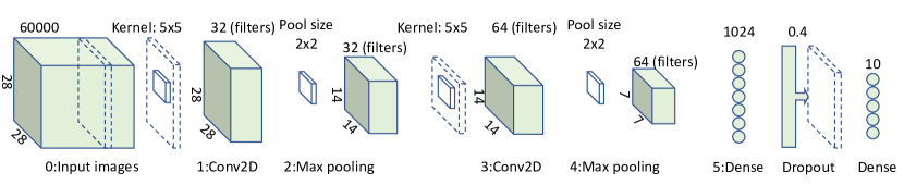
Figure 1: CNN network architecture used for all experiments

Given a set $\mathbb{M}=\{M_{1},M_{2},\ldots,M_{Z}\}$ of models, and a target dataset $T=\{\langle X_{1},Y_{1}\rangle,\langle X_{2},Y_{2}\rangle,\ldots,\langle X_{T},Y_{T}\rangle\}$, rank the $Z$ models based on a relevancy metric that identifies the “best” model for the classification task on the target labeled dataset.

With infinite resource and a large enough target dataset, an obvious approach would be applying transfer learning to retrain all model zoo models or even train new models from scratch. However, given the scarcity of labeled target datasets as well as the resource costs, such an approach does not scale. Hence, there is need for a computationally efficient approach to estimate model performance on a target dataset without having access to a large number of labeled samples. Basing model suitability on the discriminating power of models and a computationally efficient metric to measure the discriminating power is the key contribution of this paper. We formally define the problem and the metric in the following.

In general, a neural network consists of layers $0\leq n\leq N$, where $N$ is the number of parameterized layers in the network. Neurons in layer $n$ produce latent-space output $L^{n}$ by applying a pre-defined function $f_{n}$ to the outputs of the previous layer $L^{n-1}$, thus $L^{n}=f_{n}(L^{n-1})$. In general, the functions implement a variety of transformations, including but not limited to convolutions, weighted sum with bias, normalizations, and ReLU activations. $L^{0}$ is defined separately as the feature input vector $X_{i}$. By $f_{n}(X_{i})$, we denote output $L^{n}_{i}$ after the input $X_{i}$ is processed through all layers before $n$. Similarly, $L^{N}$ is the same as the predicted labels $Y^{{}^{\prime}}$ with $Y$ being the ground-truth labels.

With $K$ classes, $T$ labeled inputs in the target dataset, centroid $C_{k}^{n}$ on the outputs of layer $n$ of class $k$ is defined as follows.

$$C_{k}^{n}=\sum\limits_{i=1}^{T}\frac{L^{n}_{i}|Y_{i}=k}{T}$$ (1)

Intuitively, a discriminating model should place similar inputs closer together and as far away from other clusters as possible. We apply Silhouette’s coefficient $SC$ on the layer $n$ outputs $L^{n}$ defined as follows in terms of the intra-cluster (cohesion) and inter-cluster distance (separation) measures $a$ and $b$, respectively.

$$SC(L^{n},Y)=\sum\limits_{i=1}^{T}\frac{\frac{b(L^{n}_{i})-a(L^{n}_{i})}{max(a(L^{n}_{i}),b(L^{n}_{i}))}}{T}$$ (2)

Mean intra-cluster distance $a$ is defined relative to a point $L^{n}_{i}$ and all other points $L^{n}_{j}$ in the same class as $L^{n}_{i}$ as shown in Equation 3. Mean intra-cluster distance $b$ for a given point $L^{n}_{i}$ is simply the distance to the centroid of the nearest class as shown in Equation 4. $C_{k}^{n*}$ indicates the centroid of the closest class to $L^{n}_{i}$.

$$a(L^{n}_{i})=\sum\limits_{j=1}^{T}\frac{dist(L^{n}_{i},L^{n}_{j})|Y_{i},Y_{j}=k,i\neq j}{T}$$ (3)

$$b(L^{n}_{i})=dist(L^{n}_{i}-C_{k}^{n*})|Y_{i}\neq k$$ (4)

As $a$ and $b$ need to be computed for all points $L^{n}_{i}\in L^{n}$, computing SC involves $T^{2}$ distance computations on the latent-space projections $L^{n}$. A variety of distance measures $dist$ can be applied, we use cosine distance in this paper due to its robustness in high-dimensional spaces. An ideal model generates latent-space projections $L^{n}$ that maximize $b$ and minimize $a$, yielding SC score close to $1$. When a model cannot discriminate well across classes in $X$, $b$ and $a$ are similar, yielding SC score close to $0$. In the worst case, a model may discriminate within a class but not across classes, yielding a negative SC score.

3 neuralRank Algorithm

Input: Target dataset $(X,Y)$, Models $\mathbb{M}$

Input: Layer $n$, Projection dimensionality $D$

Output: Sorted SC scores $SC_{M}$ for all $M\in\mathbb{M}$

$SC_{list}\leftarrow\varnothing$

foreach $M\in\mathbb{M}$ do

       $N\leftarrow M$.layers

       if $n\leq N$ then

             $L^{n}\leftarrow M_{n}(X)$

             $PCA_{n}\leftarrow PCA(L^{n},D)$

             $SC_{M}\leftarrow SC(PCA_{n},Y)$

             $SC_{list}\leftarrow SC_{list}\cup SC_{M}$

            

       end if

      else

             Raise Error

       end if

      

end foreach

return Sort($SC_{list}$)

Algorithm 1 neuralRank algorithm

The algorithm involves computing SC score on latent-space projections at a chosen layer $n$ for all models in the model zoo, given a target dataset $(X,Y)$. Later, we show via experiments that typically, choosing the last dense layer works well as it captures the richest features in the inputs. No knowledge of how the models were trained or network architecture of models is assumed.

Algorithm 1 outlines the main steps of the neuralRank algorithm. Apart from the target dataset and the model repository, two parameters are needed: (1) $n$ is the chosen latent-space layer and (2) $D$ is the dimensionality to which $L^{n}$ needs to be reduced to. Latent-space outputs commonly have a large number of dimensions and distance measures do not work well on high-dimensional vectors. To overcome this, PCA is applied on the outputs $L^{n}$ to reduce the dimensionality down to $D$ and SC is measured on the reduced PCA projections.

4 Experimental Evaluation

We evaluate neuralRank on the datasets from three separate domains: MNIST hand-written digit images LeCun and Cortes (2010), Fashion apparel images Xiao et al. (2017), and CIFAR10 birds, animals, and vehicles images Krizhevsky et al. (2009). Both MNIST and fashion have $28\times 28$ grey scale images whereas CIFAR10 has $32\times 32$ color images that we resize to $28\times 28$ grey scale. Each of the datasets have 10 classes with 60K images in the training set and 10K images in the validation set. The validation sets from each of the datasets are used in all of the experiments. In the first set of experiments, the same CNN-based network architecture as shown in Figure 1 is used for training the models for each dataset. Later, we also experiment with a different architecture. A dropout rate of $0.4$ is applied on the last dense layer for regularization. All models are trained with learning rate of $0.001$ and cross-entropy loss. By default, $D=10$ is used in the PCA reduction step.

Model name	Training Dataset	Training Classes
$M_{10}$	MNIST	all
$M_{0-4}$	MNIST	0-4
$M_{5-9}$	MNIST	5-9
$F_{10}$	Fashion	all
$F_{0-4}$	Fashion	0-4
$F_{5-9}$	Fashion	5-9
$C_{10}$	CIFAR10	all
$C_{0-4}$	CIFAR10	0-4
$C_{5-9}$	CIFAR10	5-9

Table 1: Model zoo: 9 models, 3 datasets

To emulate a model zoo with models having varying degree of domain differences, three training subsets are created with samples from: (1) all classes, (2) first five classes, and (3) the remaining classes. Table 1 describes all the models in the model zoo. In the following, we investigate these questions via experiments.

• What latent-space layer should the neuralRank scores be based on?

• Is neuralRank independent of domains?

• How well does the neuralRank ranking match actual model performance?

• How sensitive are the results to the choice of $D$ in the PCA dimensionality reduction step?

• Is neuralRank independent of network architecture?

• How sensitive are the results to the dimensionality of the chosen layer?

4.1 Q₁: Latent-space layers

	$L^{0}$	$L^{1}$	$L^{2}$	$L^{3}$	$L^{4}$	$L^{5}$
$M_{10}$	0.346	0.361	0.396	0.480	0.548	0.784
$M_{0-4}$	0.346	0.369	0.409	0.477	0.544	0.821
$M_{5-9}$	0.346	0.360	0.393	0.391	0.455	0.463
$F_{10}$	0.346	0.306	0.343	0.275	0.359	0.248
$F_{0-4}$	0.346	0.328	0.366	0.257	0.356	0.276
$F_{5-9}$	0.346	0.276	0.315	0.272	0.350	0.210
$C_{10}$	0.346	0.329	0.367	0.313	0.368	0.293
$C_{0-4}$	0.346	0.351	0.380	0.337	0.394	0.315
$C_{5-9}$	0.346	0.324	0.361	0.325	0.389	0.303

Table 2: SC scores based on projections at $L^{0}$–$L^{5}$

We test neuralRank with latent-space projections at each layer to find the layer at which the scores of the most suitable models exhibit the sharpest contrast with the rest of the models. Silhouette’s coefficient (SC) defined in Eq 2, is applied to rank all models in the zoo, assuming a target dataset of MNIST inputs with classes $0-4$. Table 2 shows SC scores across $L^{0}-L^{5}$ (layer indices from Figure 1) with top-3 ranked models highlighted. The MNIST models consistently achieve the highest scores, which is not surprising given the target dataset. Importantly, the SC scores on first few layers do not exhibit much contrast whereas the last dense layer shows the sharpest contrast. This is expected because the level of abstraction increases with higher layers. We shall focus on $L^{5}$ for subsequent experiments.

4.2 Q₂: Domain independence

$M_{10}$	$M_{0-4}$	$M_{5-9}$	$F_{10}$	$F_{0-4}$	$F_{5-9}$	$C_{10}$	$C_{0-4}$	$C_{5-9}$
0.099	0.081	0.061	0.499	0.540	0.082	0.212	0.182	0.180

Table 3: SC scores on $L^{5}$ projections of Fashion inputs with classes $0-4$

$M_{10}$	$M_{0-4}$	$M_{5-9}$	$F_{10}$	$F_{0-4}$	$F_{5-9}$	$C_{10}$	$C_{0-4}$	$C_{5-9}$
0.862	0.871	0.859	0.942	0.943	0.875	0.892	0.886	0.883

Table 4: Accuracy of transfer learned models on the target dataset Fashion $0-4$

If neuralRank is indeed domain independent, rankings should not necessarily follow domain boundaries. Hence, we should be able to find cases where models outside of the domain of the target dataset are found to be more suitable than the ones matching the domain. Results in Table 2 follow along the domain boundaries and hence do not help answer this question. In the next experiment, we choose a target dataset of Fashion inputs with classes $0-4$ and observe the SC scores on layer $5$. Table 3 shows the results with top-3 ranked models highlighted. The top-2 ranks go to $F_{0-4}$ and $F_{10}$ and follow along the domain boundary. However, the third rank goes to $C_{0-4}$, which is a completely different domain (animals and vehicles) and has a clearly better score than $F_{5-9}$. One explanation is that CIFAR10 being a richer and noisier dataset, CIFAR models have been forced to learn to discriminate with richer features and such discriminatory power is domain independent.

4.3 Q₃: Ranking and model performance

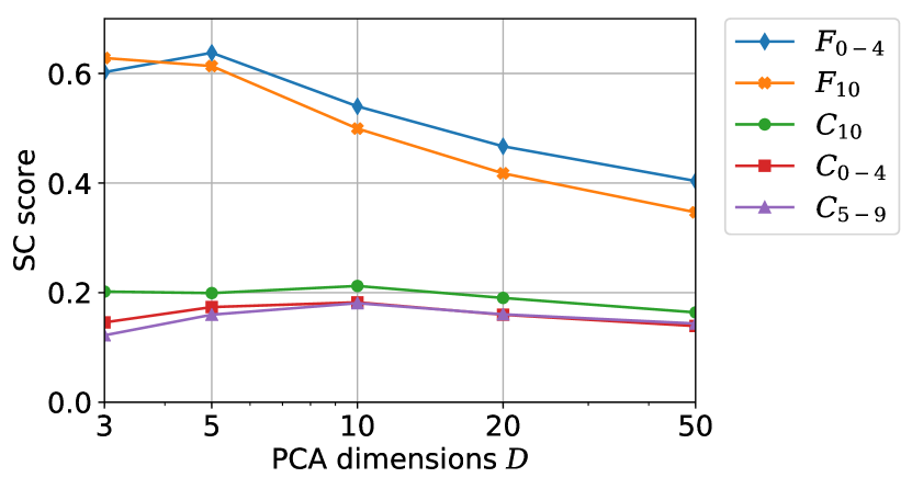
Figure 2: SC scores of top-5 models from Table 3 on $L^{5}$ with varying PCA dimensions $D$

Although the above SC score ranking results make sense, whether or not the high-ranked models actually perform well on the target datasets remains to be validated. To validate this, with the same target dataset as in Section 4.2, i.e., Fashion inputs with classes $0-4$, we apply the standard transfer learning technique of freezing weights on all layers except the logits layer. As a result, logits layer of each of the models in the zoo is retrained to correspond to the classes in the target dataset. Table 4 reports the prediction accuracy of each of the transferred models on the target dataset. The ranking of models based on SC for layer $5$ in Table 3 matches well the ranking of models based on accuracy. This result validates that SC scores can reliably predict model performance.

Although the above results establish the power of SC score experimentally, explaining why it works is important as well. Since the SC score measures the discriminatory power of models, higher rank should correspond to better discrimination. To explain this visually, Figure 3 depicts 3-dimensional PCA of the latent-space projections $L^{0}$, $L^{2}$, and $L^{5}$ of Fashion inputs with classes 0-4 using $F_{0-4}$, $C_{10}$, and $F_{5-9}$ models (ranks 1, 3, and 7 in Table 3). Color indicates class labels.

As expected, for all three models, $L^{5}$ shows the best discrimination among classes. More importantly, $F_{0-4}$ (rank 1) shows a much better discrimination than the other two models. Similarly, $C_{10}$ (rank 3) shows better discrimination than $F_{5-9}$ (rank 7), explaining why it should rank higher even though it was trained on a completely different domain.

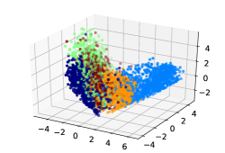
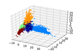
(a) $F_{0-4}$, $L^{0}$	(b) $F_{0-4}$, $L^{2}$	(c) $F_{0-4}$, $L^{5}$
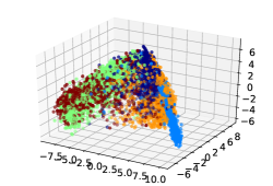
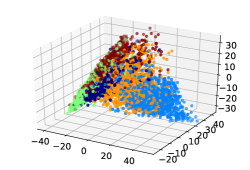
(d) $C_{10}$, $L^{0}$	(e) $C_{10}$, $L^{2}$	(f) $C_{10}$, $L^{5}$
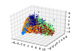
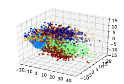
(g) $F_{5-9}$, $L^{0}$	(h) $F_{5-9}$, $L^{2}$	(i) $F_{5-9}$, $L^{5}$

Figure 3: 3D PCA visualization of latent-space projections of Fashion 0-4 inputs on $F_{0-4}$, $C_{10}$, and $F_{5-9}$

	$M_{10}^{l}$	$M_{0-4}^{l}$	$M_{5-9}^{l}$	$F_{10}^{l}$	$F_{0-4}^{l}$	$F_{5-9}^{l}$	$C_{10}^{l}$	$C_{0-4}^{l}$	$C_{5-9}^{l}$
MNIST SC score	0.671	0.723	0.419	0.226	0.231	0.189	0.301	0.305	0.304
MNIST Accuracy	0.998	0.998	0.992	0.987	0.975	0.977	0.986	0.982	0.986
Fashion SC score	0.174	0.134	0.107	0.418	0.436	0.170	0.235	0.195	0.212
Fashion Accuracy	0.881	0.864	0.868	0.939	0.939	0.878	0.883	0.855	0.876

Table 5: SC scores at $L^{3}$ and accuracy after transfer learning on lite models

	$F_{10}$	$F_{0-4}$	$C_{10}$	$C_{0-4}$	$C_{5-9}$	$F_{10}^{512}$	$F_{0-4}^{512}$	$C_{10}^{512}$	$C_{0-4}^{512}$	$C_{5-9}^{512}$
SC score	0.499	0.540	0.212	0.182	0.180	0.476	0.561	0.191	0.185	0.160
Accuracy	0.940	0.940	0.893	0.881	0.879	0.946	0.946	0.851	0.863	0.868

Table 6: SC scores at $L^{5}$ on Fashion inputs with 0–4 classes and accuracy after transfer learning on models with $512$ neurons in $L^{5}$

4.4 Q₄: Sensitivity to PCA dimensionality

As described in Section 3, a key step before computing SC scores is to reduce the dimensionality of latent-space projections to $D$ and avoid distance measurements on high-dimensional vectors. Hence, it is important to show that the results are not highly-sensitive to choice of $D$ and choosing a reasonable $D$ is trivial. Figure 2 shows changes to SC scores on $L^{5}$ with Fashion inputs having classes 0-4, with varying values of $D$ for the top-5 models from Table 3. Line cross-overs correspond to changes in ranking results. As is evident from the plot, ranking results do not change across a large range of $D$ values, generally in the ballpark of $5-50$, which is about two-orders of magnitude fewer dimensions than the original vector with 1024 dimensions for $L^{5}$. The lines do cross-over for very small and very large values of $D$, which is expected.

4.5 Q₅: Network architecture independence

All of the results so far are based on the architecture shown in Figure 1 and do not demonstrate network architecture independence on their own. In this experiment, we modify the architecture by dropping the second convolutional and max-pool layers and train nine more models with the same training set and algorithms as before. We call this the lite models and denote them as before with the lite annotation, e.g., $M_{10}^{l}$ is a lite version of $M_{10}$. Next, we repeat the ranking experiments on the new models with the same target datasets: (1) MNIST inputs with classes $0-4$ and (2) Fashion inputs with classes $0-4$. Table 5 shows the SC score on the last dense layer $L^{3}$ for both target datasets along with the actual accuracy after re-training the logits layer. Clearly, ranking and accuracy results on lite models match previous results, confirming that regardless of the network architecture, SC score is a relaible predictor of model performance. Further, taking the results of Tables 3, 4, and 5 together, ranking of all 18 models based on SC score matches the ranking based on the accuracy results.

4.6 Q₆: Dimensionality of the chosen layer

In the above experiments, the last dense layer outputs ($L^{5}$ in the original models and $L^{3}$ in the lite models) had the same dimensionality of 1024 neurons (as shown in Figure 1). As the dimensionality of the chosen layer may vary greatly in practice, it is important to study how sensitive neuralRank is to differences in the dimensioanlity of the chosen layer. To test this, we create a model zoo consisting of the top-5 best performing models from Table 3, modify layer 5 to have 512 neurons, and train five more models with the modified layer 5. Table 6 shows the SC scores and accuracy results after transfer learning on all ten models. The new models with 512 neurons are annotated with $512$, i.e., $F_{10}^{512}$ is the modified version of $F_{10}$. As the results show, regardless of the dimensions in $L^{5}$, top-5 models according to the SC score are also the top-5 models based on actual accuracy performance.

5 Related Work

This paper is the first to introduce the notion of searching across models generated by neural networks. As such, we believe that the closest relevant work is that of transfer learning, where the goal is to understand which layers are applicable to a new dataset and “transfer” these to a “new” network. Several papers have explored this area, a few key ones are Yosinski et al. (2014); Han et al. (2015). The key premise of transfer learning is to determine which portions of an existing neural network can be reused and to what extent. The reusability depends on the application domain. For example, Yosinski et al. (2014); Sun et al. (2014) show that many of the initial layers of a deep neural network trained for specific image and video classification tasks are applicable to other tasks (different from the one that they were trained on). Another recent example is in the domain of Natural Language Processing, where models such as BERT Devlin et al. (2018), ELMo Peters et al. (2018), and ULMFiT Howard and Ruder (2018) are fine tuned to be used for various text problems. The success of transfer learning in these domains shows that certain portions of neural networks can be “frozen” and reused. However, these fall short of addressing which models are the best suited for the problem at hand. This paper builds on concepts from transfer learning and shows that we can use a simple cluster quality metric to determine which components of the neural network are applicable in a structured manner.

The next relevant work is that of interpretability, where the goal is to better understand what each layer of the neural network is “doing”. One of the approaches to interpretability is to use visualization  Olah et al. (2017, 2018); Krause et al. (2016); Bau et al. (2017), where each of the layers of the neural network is visualized as an image. This approach is quite useful when working with image data, which provides some insights into what each layer is capturing. For example, as is well-illustrated in Olah et al. (2017), the initial layers are capturing edges, followed by textures and patterns, then parts and finally objects (leading to classes). One notices that as we gradually go up the layers, the complexity of the recognition grows. These visualizations are quite useful for humans to understand why a network is working as observed and what kind of features it is learning in each layer. However, the work on visualization does not quantify the applicability of layers for a different task.

6 Conclusions

As applications of deep learning models grow, large repositories of models are springing up. This paper introduced the problem of searching and ranking such model repositories. A novel technique for ranking models is proposed based on Silhouette’s coefficient on latent-space projections. A key new insight is that the discriminatory power of a model is a reliable indicator of model suitability regardless of the domain or the training method. The proposed technique also lends itself well to a visual explanation of rankings. Through rigorous experiments, the ranking algorithm is shown to work well across domains, network architectures, and dimensionality of the chosen latent-space projections. Most importantly, the ranking results correspond well to the actual model performance after transfer learning.

Although these are promising results, this paper represents a first step in solving the broader problem of model search. A key assumption needs to be relaxed for solving the broader problem: an unsupervised technique for model search wherein the target dataset is not labeled. This is a significant problem because in many applications, acquiring sufficient amount of labeled data is costly or even infeasible. Also, this is a challenging problem because model suitability is relative to the needs of an application and labels represent the application requirements, e.g., classifying vehicles in images versus classifying landmarks.

References

- Bau et al. [2017] David Bau, Bolei Zhou, Aditya Khosla, Aude Oliva, and Antonio Torralba. Network dissection: Quantifying interpretability of deep visual representations. In Computer Vision and Pattern Recognition, 2017.
- Devlin et al. [2018] Jacob Devlin, Ming-Wei Chang, Kenton Lee, and Kristina Toutanova. BERT: pre-training of deep bidirectional transformers for language understanding. CoRR, abs/1810.04805, 2018.
- Han et al. [2015] Song Han, Jeff Pool, John Tran, and William Dally. Learning both weights and connections for efficient neural network. In C. Cortes, N. D. Lawrence, D. D. Lee, M. Sugiyama, and R. Garnett, editors, Advances in Neural Information Processing Systems 28, pages 1135–1143. 2015.
- Howard and Ruder [2018] Jeremy Howard and Sebastian Ruder. Fine-tuned language models for text classification. CoRR, abs/1801.06146, 2018.
- Krause et al. [2016] Josua Krause, Adam Perer, and Kenney Ng. Interacting with predictions: Visual inspection of black-box machine learning models. In Proceedings of the 2016 CHI Conference on Human Factors in Computing Systems, pages 5686–5697, 2016.
- Krizhevsky et al. [2009] Alex Krizhevsky, Vinod Nair, and Geoffrey Hinton. Cifar-10 (canadian institute for advanced research). 2009.
- LeCun and Cortes [2010] Yann LeCun and Corinna Cortes. MNIST handwritten digit database. 2010.
- Olah et al. [2017] Chris Olah, Alexander Mordvintsev, and Ludwig Schubert. Feature visualization. Distill, 2017. https://distill.pub/2017/feature-visualization.
- Olah et al. [2018] Chris Olah, Arvind Satyanarayan, Ian Johnson, Shan Carter, Ludwig Schubert, Katherine Ye, and Alexander Mordvintsev. The building blocks of interpretability. Distill, 2018. https://distill.pub/2018/building-blocks.
- Peters et al. [2018] Matthew E. Peters, Mark Neumann, Mohit Iyyer, Matt Gardner, Christopher Clark, Kenton Lee, and Luke Zettlemoyer. Deep contextualized word representations. In Proc. of NAACL, 2018.
- Rousseeuw [1987] Peter Rousseeuw. Silhouettes: A graphical aid to the interpretation and validation of cluster analysis. J. Comput. Appl. Math., 20(1):53–65, November 1987.
- Sun et al. [2014] Yi Sun, Xiaogang Wang, and Xiaoou Tang. Deep learning face representation from predicting 10,000 classes. In The IEEE Conference on Computer Vision and Pattern Recognition (CVPR), June 2014.
- Xiao et al. [2017] Han Xiao, Kashif Rasul, and Roland Vollgraf. Fashion-mnist: a novel image dataset for benchmarking machine learning algorithms. CoRR, abs/1708.07747, 2017.
- Yosinski et al. [2014] Jason Yosinski, Jeff Clune, Yoshua Bengio, and Hod Lipson. How transferable are features in deep neural networks? In Z. Ghahramani, M. Welling, C. Cortes, N. D. Lawrence, and K. Q. Weinberger, editors, Advances in Neural Information Processing Systems 27, pages 3320–3328. 2014.