Matrix Completion via Nonconvex Regularization: Convergence of the Proximal Gradient Algorithm

Abstract

Matrix completion has attracted much interest in the past decade in machine learning and computer vision. For low-rank promotion in matrix completion, the nuclear norm penalty is convenient due to its convexity but has a bias problem. Recently, various algorithms using nonconvex penalties have been proposed, among which the proximal gradient descent (PGD) algorithm is one of the most efficient and effective. For the nonconvex PGD algorithm, whether it converges to a local minimizer and its convergence rate are still unclear. This work provides a nontrivial analysis on the PGD algorithm in the nonconvex case. Besides the convergence to a stationary point for a generalized nonconvex penalty, we provide more deep analysis on a popular and important class of nonconvex penalties which have discontinuous thresholding functions. For such penalties, we establish the finite rank convergence, convergence to restricted strictly local minimizer and eventually linear convergence rate of the PGD algorithm. Meanwhile, convergence to a local minimizer has been proved for the hard-thresholding penalty. Our result is the first shows that, nonconvex regularized matrix completion only has restricted strictly local minimizers, and the PGD algorithm can converge to such minimizers with eventually linear rate under certain conditions. Illustration of the PGD algorithm via experiments has also been provided. Code is available at https://github.com/FWen/nmc.

I Introduction

Matrix completion deals with the problem of recovering of a matrix from its partially observed (may be noisy) entries, which has attracted considerable interest recently [1]–[4]. The matrix completion problem arises in many applications in signal processing, image/video processing, and machine learning, such as rating value estimation in recommendation system [7], friendship prediction in social network, collaborative filtering [8], image processing [6], [10], video denoising [12], [13], system identification [14], multiclass learning [15], [16], and dimensionality reduction [17]. Specifically, the goal of matrix completion is to recover a matrix ${\bf{M}}\in{\mathbb{R}^{m\times n}}$ from its partially observed (incomplete) entries

$${{\bf{Y}}_{i,j}}={{\bf{M}}_{i,j}},~{}~{}~{}~{}(i,j)\in\Omega$$ (1)

where $\Omega\subset[1,\cdots,m]\times[1,\cdots,n]$ is a random subset. Obviously, the completion of an arbitrary matrix is an ill-posed problem. To make the problem well-posed, a commonly used assumption is that the underlying matrix ${\bf{M}}$ comes from a restricted class, e.g., low-rank. Exploiting the low-rank structure of the matrix is a powerful method.

Modeling the matrix completion problem as a low-rank matrix recovery problem, a natural formulation is to minimize the rank of ${\bf{M}}$ under the linear constraint (1) as

$$\begin{split}&\mathop{{\rm{minimize}}}\limits_{\bf{X}}{\rm{rank}}({\bf{X}})\\ &\textrm{subject to }~{}~{}{{\mathcal{P}}_{\Omega}}({\bf{X}})={{\bf{Y}}_{\Omega}}\end{split}$$ (2)

where ${{\mathcal{P}}_{\Omega}}:{\mathbb{R}^{m\times n}}\to{\mathbb{R}^{m\times n}}$ denotes projection onto the set $\Omega$, and ${{\bf{Y}}_{\Omega}}={{\mathcal{P}}_{\Omega}}({\bf{Y}})$. While the nonconvex rank minimization problem (2) is highly nonconvex and difficult to solve, a popular convex relaxation method is to replace the rank function by its convex envelope, the nuclear norm ${\left\|\cdot\right\|_{*}}$,

$$\begin{split}&\mathop{{\rm{minimize}}}\limits_{\bf{X}}{\left\|{\bf{X}}\right\|_{*}}\\ &\textrm{subject to }~{}~{}{{\mathcal{P}}_{\Omega}}({\bf{X}})={{\bf{Y}}_{\Omega}}.\end{split}$$ (3)

In most realistic applications, entry-wise noise is inevitable. Taking entry-wise noise into consideration, a robust variant of (3) is

$$\begin{split}&\mathop{{\rm{minimize}}}\limits_{\bf{X}}{\left\|{\bf{X}}\right\|_{*}}\\ &\textrm{subject to }~{}~{}\left\|{{{\bf{Y}}_{\Omega}}-{{\mathcal{P}}_{\Omega}}({\bf{X}})}\right\|_{F}^{2}\leq\varepsilon\end{split}$$ (4)

where $\varepsilon>0$ is the noise tolerance. This constrained formulation (4) can be converted into an unconstrained form as

$$\mathop{{\rm{minimize}}}\limits_{\bf{X}}\frac{1}{2}\left\|{{{\bf{Y}}_{\Omega}}-{{\mathcal{P}}_{\Omega}}({\bf{X}})}\right\|_{F}^{2}+\lambda{\left\|{\bf{X}}\right\|_{*}}$$ (5)

where $\lambda>0$ is a regularization parameter related to the noise tolerance parameter $\varepsilon$ in (4). The unconstrained formulation is favorable in some applications as existing efficient first-order convex algorithms, such as alternative direction method of multipliers (ADMM) or proximal gradient descent (PGD) algorithm, can be directly applied. Even in the noise free case, the solution of (5) can accurately approach that of (3) via choosing a sufficiently small value of $\lambda$, since the solution of (5) satisfies ${\left\|{{{\bf{Y}}_{\Omega}}-{{\mathcal{P}}_{\Omega}}({\bf{X}}))}\right\|_{F}}\to 0$ as $\lambda\to{\rm{0}}$. The problems (3) and (4) can be recast into semi-definite program (SDP) problems and solved to global minimizer by well-established SDP solvers when the matrix dimension is not large. For problems with larger size, more efficient first-order algorithms have been developed based on the formulation (5), e.g., variants of the proximal gradient method [19], [20].

Besides the tractability of the convex formulations (3)–(5) employing nuclear norm, theoretical guarantee provided in [1], [2], [21], [22] demonstrated that under certain conditions, e.g., when the low-rank matrix ${\bf{M}}$ satisfies an incoherence condition and the observed entries are uniformly randomly sampled, ${\bf{M}}$ can be exactly recovered from a small portion of its entries with high probability by using the nuclear norm regularization. However, the nuclear norm regularization has a bias problem and would introduce bias to the recovered singular values [23]–[25]. To alleviate the bias problem and achieve better recovery performance, a nonconvex low-rank penalty, such as the Schatten-$q$ norm (which is in fact the $\ell_{q}$ norm of the matrix singular values with $0<q<1$), smoothly clipped absolute deviation (SCAD), minimax concave (MC), or firm-thresholding penalty can be used. In the past a few years, nonconvex regularization has shown better performance over convex regularization in many sparse and low-rank recovery involved applications. These applications include compressive sensing, sparse regression, sparse demixing, sparse covariance and precision matrix estimation, and robust principal component analysis [9], [26].

In this work, we consider the following formulation for matrix completion

$$\mathop{{\rm{minimize}}}\limits_{\bf{X}}F({\bf{X}}):=\frac{1}{2}\left\|{{{\bf{Y}}_{\Omega}}-{{\mathcal{P}}_{\Omega}}({\bf{X}})}\right\|_{F}^{2}+\lambda\bar{R}({\bf{X}})$$ (6)

where $\bar{R}$ is a generalized nonconex low-rank promotion penalty. For the particular case of $\bar{R}$ being the nuclear norm, i.e., $\bar{R}(\cdot)={\left\|\cdot\right\|_{*}}$, this formulation reduces to (5). Existing works considering the nonconvex formulation (6) include [27]–[31]. In [27], [28], the Schatten-$q$ norm has been considered and PGD methods have been proposed. In [29], using a smoothed Schatten-$q$ norm, an iteratively reweighted algorithm has been designed for (6), which involves solving a sequence of linear equations. Another iteratively reweighted algorithm for Schatten-$q$ norm regularized matrix minimization problem with a generalized smooth loss function has been investigated in [30]. More recently in [31], $\bar{R}$ being the MC penalty has been considered and an ADMM algorithm has been developed.

Besides, for the linearly constrained formulation, an iterative algorithm employing Schatten-$q$ norm, which monotonically decreasing the objective, has been proposed in [32]. Meanwhile, a truncated nuclear norm has been used in [33]. Then, robust matrix completion using Schatten-$q$ regularization has been considered in [34]. Moreover, it has been shown in [35] that, the sufficient condition for reliable recovery of Schatten-$q$ norm regularization is weaker than that of nuclear norm regularization.

Among the nonconvex algorithms for the problem (6), only subsequence convergence of the methods [27]–[31] have been proved. In fact, based on the recent convergence results for nonconvex and nonsmooth optimization [36]–[38], global convergence of the PGD algorithm [27], [28] and the ADMM algorithm [31] to a stationary point can be guaranteed under some mild conditions. However, for a nonconvex $\bar{R}$, whether these algorithms converge to a local minimizer is still unclear. Meanwhile, for the problem (6), linear convergence rate of the PGD algorithm has been established when $\bar{R}$ is the nuclear norm under certain conditions [39], [40], but the convergence rate of PGD in the case of a nonconvex $\bar{R}$ is still an open problem.

To address these problems, this work provides a thorough analysis on the PGD algorithm for the matrix completion problem (6) using a generalized nonconvex penalty. The main contributions are as follows.

I-A Contribution

First, we derived some properties on the gradient and Hessian of a generalized low-rank penalty, which are important for the convergence analysis. Then, for a popular and important class of nonconvex penalties which have discontinuous thresholding functions, we have established the following convergence properties for the PGD algorithm under certain conditions:

1) rank convergence within finitely many iterations;

2) convergence to a restricted strictly local minimizer;

3) convergence to a local minimizer for the hard-thresholding penalty;

4) an eventually linear convergence rate.

As the singular value thresholding function is implicitly dependent on the low-rank matrix, the derivation is nontrivial. Finally, illustration of the PGD algorithm via inpainting experiments has been provided.

It is worth noting that, there exist a line of recent works on factorization based nonconvex algorithms, e.g., [5], [11], [18]. It has been shown that the nonconvex objective function has no spurious local minimum, and efficient nonconvex optimization algorithms can converge to local minimum. While these works focus on matrix factorization based methods, this work considers the general matrix completion problem (6). Our result is the first explains that the nonconvex matrix completion problem (6) only have restricted strictly local minimum, and the PGD algorithm can converge to such minimum with eventually linear rate under certain conditions.

Outline: The rest of this paper is organized as follows. Section II introduces the proximity operator for generalized nonconvex penalty, and reviews the PGD algorithm for matrix completion. Section III provides convergence analysis of the PGD algorithm. Section IV provides experimental results on inpainting. Finally, section V ends the paper with concluding remarks.

TABLE I: Proximity operator for some popular regularization penalties.

Penalty name	Penalty formulation	Proximity operator
(i) Hard thresholding	${R}(x)={\rm{|}}x{{\rm{|}}_{0}}$	${P_{R,\eta}}(t)=\left\{{\begin{array}[]{*{20}{l}}{0,}&{|t|\leq\sqrt{2/\eta}}\\ {t,}&{|t|\geq\sqrt{2/\eta}}\end{array}}\right.$
(ii) Soft thresholding	${R}(x)={\rm{|}}x{\rm{|}}$	${P_{R,\eta}}(t)={\rm{sign}}(t)\max\left\{{|t|-1/\eta,0}\right\}$
(iii) $\ell_{q}$-norm	${R}(x)={\rm{|}}x{{\rm{|}}^{q}}$, $0<q<1$	${P_{R,\eta}}(t)=\left\{{\begin{array}[]{*{20}{l}}{0,}&{{\rm{|}}t{\rm{|}}\leq\tau}\\ {{{\rm{sign}}(t){h^{-1}}({\rm{|}}t{\rm{|}})},}&{{\rm{|}}t{\rm{|}}\geq\tau}\end{array}}\right.$ where $h(x)=q{x^{q-1}}/\eta+x$, $\tau={\beta_{\eta}}+q\beta_{\eta}^{q-1}/\eta$, ${\beta_{\eta}}={[2(1-q)/\eta]^{1/(2-q)}}$

Notations: For a matrix ${\bf{X}}\in{\mathbb{R}^{m\times n}}$, ${\rm{rank}}({\bf{X}})$, ${\rm{tr}}({\bf{X}})$, ${\left\|{\bf{X}}\right\|_{F}}$ and $\mathcal{R}({\bf{X}})$ stand for the rank, trace, Frobenius norm and range space of ${\bf{X}}$, respectively, whilst ${\sigma_{i}}({\bf{X}})$ denotes the $i$-th largest singular value, and

$${\bm{\sigma}}({\bf{X}}) :={[{\sigma_{1}}({\bf{X}}),\cdots,{\sigma_{\min(m,n)}}({\bf{X}})]^{T}}$$

$${{\bm{\sigma}}_{r}}({\bf{X}}) :={[{\sigma_{1}}({\bf{X}}),\cdots,{\sigma_{r}}({\bf{X}})]^{T}}$$

$${{\bm{\sigma}}_{r\bot}}({\bf{X}}) :={[{\sigma_{r+1}}({\bf{X}}),\cdots,{\sigma_{\min(m,n)}}({\bf{X}})]^{T}}.$$

For a symmetric real matrix ${\bf{X}}$, ${\lambda_{\max}}({\bf{X}})$ and ${\lambda_{\min}}({\bf{X}})$ respectively denote the maximal and minimal eigenvalues, whilst ${\bm{\lambda}}({\bf{X}})$ contains the descendingly ordered eigenvalues. ${\bf{X}}\succeq{\bf{0}}$ and ${\bf{X}}\succ{\bf{0}}$ mean that ${\bf{X}}$ is semi-definite and positive definite, respectively. ${\bf{X}}(i,j)$ denotes the $(i,j)$-th element. ${\rm{vec}}(\cdot)$ is the “vectorization” operator stacking the columns of the matrix one below another. ${\bf{diag}}({\bf{v}})$ represents the diagonal matrix generated by the vector ${\bf{v}}$, ${\rm{diag}}({\bf{X}})$ represents the vector containing the diagonal elements of ${\bf{X}}$. ${\left\|\cdot\right\|_{2}}$ denotes the Euclidean norm. $\odot$ and $\otimes$ denote the Hadamard and Kronecker product, respectively. $\langle\cdot,\cdot\rangle$ and ${(\cdot)^{T}}$ denote the inner product and transpose, respectively. ${\rm{sign}}(\cdot)$ denotes the sign of a quantity with ${\rm{sign}}(0){\rm{=}}0$. ${{\bf{I}}_{m}}$ is an $m\times m$ identity matrix. ${\bf{0}}$ is a zero vector or matrix with a proper size.

II Proximity Operator and Proximal Gradient Algorithm

This section introduces the proximity operator for nonconvex regularization and the PGD algorithm for the matrix completion problem (6).

II-A Proximal Operator for Nonconvex Penalties

For a proper and lower semicontinuous penalty function $R$, the corresponding proximity operator is defined as

$${P_{R,\eta}}(t)=\arg\mathop{\min}\limits_{x}\left\{{R(t)+\frac{\eta}{2}{{(x-t)}^{\rm{2}}}}\right\}$$ (7)

where $\eta>0$ is a penalty parameter.

Table I shows several popular penalties along with their thresholding functions. The proximal minimization problem (7) for many popular nonconvex penalties can be computed in an efficient manner. The hard-thresholding is a natural selection for sparsity promotion, while the soft-thresholding is of the most popular due to its convexity. The $\ell_{q}$ penalty with $0<q<1$ bridges the gap between the hard- and soft-thresholding penalties. Except for two known cases of $q=\frac{1}{2}$ and $q=\frac{2}{3}$, the proximity operator of the ${\ell_{q}}$ penalty does not have a closed-form expression, but it can be efficiently computed by an iterative method. Moreover, there also exist other nonconvex penalties, including the $q$-shrinkage [41]–[42], SCAD [43], MC [44] and firm thresholding [45].

As shown in Fig. 1, the soft-thresholding imposes a constant shrinkage on the parameter when the parameter magnitude exceeds the threshold, and, thus, has a bias problem. The hard- and SCAD thresholding are unbiased for large parameter. The other nonconvex thresholding functions are sandwiched between the hard- and the soft-thresholding, which can mitigate the bias problem of the soft-thresholding. For a generalized nonconvex penalty, we make the following assumptions.

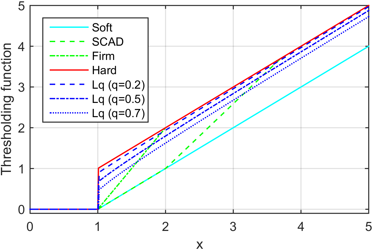
Figure 1: Thresholding/shrinkage function output (with a same threshold).

Assumption 1: ${R}$ is an even folded concave function, which satisfies the following conditions:

(i) ${R}$ is non-decreasing on $[0,\infty)$ with ${R}(0)=0$;

(ii) for any $t>0$, there exists a $c>0$ such that ${R}(|x|)\geq c{x^{2}}$ for any $|x|\in[0,t]$;

(iii) ${R}$ is ${C^{2}}$ on $(-\infty,0)\cup(0,\infty)$, and ${R^{\prime\prime}}\leq 0$ on $(0,\infty)$;

(iv) the first-order derivative ${R^{\prime}}$ is convex on $(0,\infty)$ and $\mathop{\lim}\limits_{|x|\to\infty}{R^{\prime}}(|x|)/|x|=0$.

This assumption implies that $R$ is coercive, weakly sequential lower semi-continuous in $\ell^{2}$, and responsible for sparsity promotion.

II-B Generalized Singular Value Thresholding

For a matrix ${\bf{X}}\in{\mathbb{R}^{m\times n}}$, low-rank inducing on ${\bf{X}}$ can be achieved via sparsity inducing on the singular values as

$$\bar{R}({\bf{X}}):=R({\bm{\sigma}}({\bf{X}}))=\sum\nolimits_{i=1}{R({\sigma_{i}}({\bf{X}}))}$$ (8)

where $R$ is a sparsity inducing penalty. For the particular cases of $R$ being the ${\ell_{0}}$, ${\ell_{q}}$ and ${\ell_{1}}$ norm, $\bar{R}({\bf{X}})$ become the rank, Schatten-$q$ norm and nuclear norm of ${\bf{X}}$, respectively. For such a low-rank penalty, define the corresponding proximal operator

$${\bar{P}_{\bar{R},\eta}}({\bf{T}})=\arg\mathop{\min}\limits_{\bf{X}}\left\{{\bar{R}({\bf{X}})+\frac{\eta}{2}\left\|{{\bf{X}}-{\bf{T}}}\right\|_{F}^{2}}\right\}.$$ (9)

Property 1. [Generalized singular value thresholding]: Let ${\bf{T}}={\bf{Udiag}}({\bm{\sigma}}({\bf{T}})){{\bf{V}}^{T}}$ be any full singular value decomposition (SVD) of ${\bf{T}}$, where ${\bf{U}}\in{\mathbb{R}^{m\times m}}$ and ${\bf{V}}\in{\mathbb{R}^{n\times n}}$ contain the left and right singular vectors, respectively. Then, the proximal minimization problem (9) is solved by the singular-value thresholding operator

$${\bar{P}_{\bar{R},\eta}}({\bf{T}})={\bf{U}}{\bf{diag}}\left\{{{P_{R,\eta}}({\bm{\sigma}}({\bf{T}}))}\right\}{{\bf{V}}^{T}}$$ (10)

where

$${P_{R,\eta}}({\bm{\sigma}}({\bf{T}}))={[{P_{R,\eta}}({\sigma_{1}}({\bf{T}})),\cdots,{P_{R,\eta}}({\sigma_{\min(m,n)}}({\bf{T}}))]^{T}}.$$

Although this property can be derived via straightforwardly extending Lemma 1 in [7], we provide here a completely different but more intuitive derivation of it. Assume that the minimizer ${{\bf{X}}^{*}}$ of (9) is of rank $r$ with any truncated SVD ${{\bf{X}}^{*}}={{\bf{U}}^{*}}{{\bf{\Sigma}}^{*}}{{\bf{V}}^{*T}}$, where ${{\bf{\Sigma}}^{*}}{{=}}{\bf{diag}}({{\bm{\sigma}}_{r}}({{\bf{X}}^{*}}))$. Then, the objective in (9) can be equivalently rewritten as

$$T({\bf{X}}):=R({{\bm{\sigma}}_{r}}({\bf{X}}))+\frac{\eta}{2}\left\|{{\bf{X}}-{\bf{T}}}\right\|_{F}^{2}.$$ (11)

By Assumption 1, $R$ is differential on $(0,+\infty)$, hence, $T$ is differential with respective to rank-$r$ matrix ${\bf{X}}$. Denote

$${{\bf{\Sigma}}^{*}}^{\prime}={\bf{diag}}({[R^{\prime}({\sigma_{1}}({{\bf{X}}^{*}})),\cdots,R^{\prime}({\sigma_{r}}({{\bf{X}}^{*}}))]^{T}})$$

where $R^{\prime}$ is the first-order derivative of $R$, we have (see Appendix A)

$${\nabla_{\bf{X}}}T({{\bf{X}}^{*}})={{\bf{U}}^{*}}{{\bf{\Sigma}}^{*}}^{\prime}{{\bf{V}}^{*T}}+\eta({\bf{X^{*}}}-{{\bf{U}}^{*}}{{\bf{U}}^{*T}}{\bf{TV}}{{\bf{V}}^{*T}}).$$ (12)

Let ${\nabla_{\bf{X}}}T({{\bf{X}}^{*}})={\bf{0}}$, and use ${{\bf{U}}^{*T}}{{\bf{U}}^{*}}={{\bf{I}}_{r}}$, ${{\bf{V}}^{*T}}{{\bf{V}}^{*}}={{\bf{I}}_{r}}$, it follows from (12) that

$${{\bf{\Sigma}}^{*}}^{\prime}+\eta{{\bf{\Sigma}}^{*}}-\eta{{\bf{U}}^{*T}}{\bf{T}}{{\bf{V}}^{*}}={\bf{0}}.$$

Since ${{\bf{\Sigma}}^{*}}^{\prime}$ and ${{\bf{\Sigma}}^{*}}$ are diagonal, and the columns of ${{\bf{U}}^{*}}$ (also ${{\bf{V}}^{*}}$) are orthogonal, it is easy to see that there exists a full SVD ${\bf{T}}={\bf{U\Sigma}}{{\bf{V}}^{T}}$ such that

$${\bf{U}}=[{{\bf{U}}^{*}},{\bf{U}}_{\bot}^{*}]~{}~{}~{}~{}{\rm{and}}~{}~{}~{}~{}{\bf{V}}=[{{\bf{V}}^{*}},{\bf{V}}_{\bot}^{*}].$$ (13)

Substituting these relations into (11) yields

$$T({\bf{X}}^{*})=R({{\bm{\sigma}}_{r}}({{\bf{X}}^{*}}))+\frac{\eta}{2}\left\|{{{\bm{\sigma}}_{r}}({{\bf{X}}^{*}})-{{\tilde{\bm{\sigma}}}_{T,r}}}\right\|_{2}^{2}$$ (14)

where ${\tilde{\bm{\sigma}}_{T,r}}$ contains $r$ singular values of ${\bf{T}}$. As (14) is separable, ${\{{\sigma_{i}}({{\bf{X}}^{*}})\}_{1\leq i\leq r}}$ can be solved element-wise as (7), i.e., ${\sigma_{i}}({{\bf{X}}^{*}})={P_{R,\eta}}({\tilde{\bm{\sigma}}_{T,r}}(i))$. Further, $R$ is nondecreasing on $(0,+\infty)$ by Assumption 1, hence ${P_{R,\eta}}(x)\leq{P_{R,\eta}}(y)$ for any $0<x\leq y$. Thus, ${\tilde{\bm{\sigma}}_{T,r}}$ must contain the $r$ largest singular values of ${\bf{T}}$ with a same descending order as ${{\bm{\sigma}}_{r}}({{\bf{X}}^{*}})$, i.e., ${\tilde{\bm{\sigma}}_{T,r}}={{\bm{\sigma}}_{r}}({\bf{T}})={[{\sigma_{1}}({\bf{T}}),\cdots,{\sigma_{r}}({\bf{T}})]^{T}}$. Consequently, we have ${{\bm{\sigma}}_{r}}({{\bf{X}}^{*}})={P_{R,\eta}}({{\bm{\sigma}}_{r}}({\bf{T}}))$, which together with ${P_{R,\eta}}({[{\sigma_{r+1}}({\bf{T}}),\cdots,{\sigma_{\min(m,n)}}({\bf{T}})]^{T}})={\bf{0}}$ and (13) results in (10).

II-C PGD Algorithm for Matrix Completion

PGD is a powerful optimization algorithm suitable for many large-scale problems arising in signal/image processing, statistics and machine learning. It can be viewed as a variant of majorization minimization algorithms which has a special choice for the quadratic majorization. Let

$$G({\bf{X}}):=\frac{1}{2}\left\|{{{\bf{Y}}_{\Omega}}-{{\mathcal{P}}_{\Omega}}({\bf{X}}))}\right\|_{F}^{2}.$$

The core idea of the PGD algorithm is to consider a linear approximation of $G$ at the $(k+1)$-th iteration at a given point ${{\bf{X}}^{k}}$ as

$$\begin{split}{F_{L}}({\bf{X}};{{\bf{X}}^{k}})=G({{\bf{X}}^{k}})&+\left\langle{{\bf{X}}-{{\bf{X}}^{k}},\nabla G({{\bf{X}}^{k}})}\right\rangle\\ &+\frac{L}{2}\left\|{{\bf{X}}-{{\bf{X}}^{k}}}\right\|_{F}^{2}+\lambda\bar{R}({\bf{X}})\end{split}$$ (15)

where $\nabla G({{\bf{X}}^{k}})={{\mathcal{P}}_{\Omega}}({{\bf{X}}^{k}})-{{\bf{Y}}_{\Omega}}$ and $L>0$ is a proximal parameter. Then, minimizing ${F_{L}}({\bf{X}};{{\bf{X}}^{k}})$ is a form of the proximity operator (9) as

$${{\bf{X}}^{k+1}}={\bar{P}_{\bar{R},L/\lambda}}\left({{{\bf{X}}^{k}}-\frac{1}{L}\nabla G({{\bf{X}}^{k}})}\right)$$ (16)

which can be computed as (10).

In the PGD algorithm, the dominant computational load in each iteration is the SVD calculation. To further improve the efficiency of the algorithm and make it scale well for large-scale problems, the techniques such as approximate SVD or PROPACK [7], [19] can be adopted.

III Convergence Analysis

This section investigates the convergence properties of the PGD algorithm with special consideration on the class of nonconvex penalties which have discontinuous thresholding functions. First, we make some assumptions on the discontinuous property of such threshoding functions.

Assumption 2: ${R}$ satisfies Assumption 1, and the corresponding proximity operator has a formulation as

$${P_{{R},\eta}}(t)=\left\{{\begin{array}[]{*{20}{l}}{0,}&{{\rm{|}}t{\rm{|}}\leq{\tau_{\eta}}}\\ {{\rm{sign}}(t)\rho_{\eta}^{-1}(|t|),}&{{\rm{|}}t{\rm{|}}\geq{\tau_{\eta}}}\end{array}}\right.$$ (17)

where ${\rho_{\eta}}$ is defined on $\mathbb{R}_{+}$ as ${\rho_{\eta}}:x\mapsto{R^{\prime}}(x)/\eta+x$, for any $\eta>0$ and $x>0$. ${\tau_{\eta}}>0$ is the threshold point given by ${\tau_{\eta}}={\rho_{\eta}}({\beta_{\eta}})$. ${\beta_{\eta}}=\rho_{\eta}^{-1}({\tau_{\eta}})>0$ is the “jumping” size at the threshold point. ${P_{R,\eta}}(t)$ is continuous on $\{|t|\neq{\tau_{\eta}}\}$ and the range of ${P_{{R},\eta}}(t)$ is $(-\infty,-{\beta_{\eta}}]\cup\{0\}\cup[{\beta_{\eta}},+\infty)$.

A significant property of such a nonconvex penalty is its jumping discontinuity. Typical nonconvex penalties satisfying this discontinuous property include the ${\ell_{0}}$, ${\ell_{q}}$, and log-$q$ penalties.

In the analysis, the Kurdyka-Lojasiewicz (KL) property of the objective function is used. In the convergence analysis, based on a “uniformization” result [36], using the KL property can considerably predigest the main arguments and avoid involved induction reasoning.

Definition 1. [KL property]: For a proper function $f:{\mathbb{R}^{n}}\to\mathbb{R}$ and any ${x_{0}}\in{\rm{dom}}\partial f$, if there exists $\eta>0$, a neighborhood $\mathcal{V}$ of ${x_{0}}$ and a continuous concave function $\varphi:[0,\eta)\to{\mathbb{R}_{+}}$ such that:

(i) $\varphi(0)=0$ and $\varphi$ is continuously differentiable on $(0,\eta)$ with positive derivatives;

(ii) for all $x\in\mathcal{V}$ satisfying $f({x_{0}})<f(x)<f({x_{0}})+\eta$, it holds that $\varphi^{\prime}(f(x)-f({x_{0}})){\rm{dist}}(0,\partial f(x))\geq 1$;

then $f$ is said to have the KL property at $x_{0}$. Further, if a proper closed function $f$ satisfies the KL property at all points in ${\rm{dom}}\partial f$, it is called a KL function.

Furthermore, we define the restricted strictly local minimizer as follows. Let ${\mathcal{P}}_{\Omega}^{\bot}:{\mathbb{R}^{m\times n}}\to{\mathbb{R}^{m\times n}}$ denote the projection onto the complementary set of $\Omega$.

Definition 2. [Restricted strictly local minimizer]: For a proper function $f:{\mathbb{R}^{m\times n}}\to{\mathbb{R}}$, any ${{\bf{X}}^{*}}\in{\rm{dom}}\partial f$ and a subset $\Omega\subset[1,\cdots,m]\times[1,\cdots,n]$, if there exists a neighborhood $\mathcal{V}$ of ${{\bf{X}}^{*}}$ such that for any ${\bf{X}}\in\mathcal{V}$,

$$f({\mathcal{P}_{\Omega}}({\bf{X}})+\mathcal{P}_{\Omega}^{\bot}({{\bf{X}}^{*}}))>f({{\bf{X}}^{*}})$$

${{\bf{X}}^{*}}$ is said to be a $\Omega$-restricted strictly local minimizer of $f$.

It is obvious that, if ${{\bf{X}}^{*}}$ is a strictly local minimizer of $f$, then ${{\bf{X}}^{*}}$ is a $\Omega$-restricted strictly local minimizer of $f$, but not vice versa.

Meanwhile, we provide three lemmas needed in later analysis. The first lemma is on the distance between the singular values of two matrices.

Lemma 1: For two matrices ${\bf{A}}\in{\mathbb{R}^{m\times n}}$ and ${\bf{B}}\in{\mathbb{R}^{m\times n}}$, it holds

$$\left\|{{\bm{\sigma}}({\bf{A}})-{\bm{\sigma}}({\bf{B}})}\right\|_{2}^{2}\leq\left\|{{\bf{A}}-{\bf{B}}}\right\|_{F}^{2}.$$

This result can be directly derived by extending the Hoffman-Wielandt Theorem [47], which indicates that the “distance” between the respective singular values of two matrices is bounded by the “distance” between the matrices.

The following two lemmas present some properties of the gradient and Hessian of a generalized low-rank penalty [46] (the derivation is also provided here in Appendices A and B).

Lemma 2: For a matrix ${\bf{X}}\in{\mathbb{R}^{m\times n}}$ of rank $r$, $r\leq\min(m,n)$, with any truncated SVD ${\bf{X}}={\bf{U\Sigma V}}^{T}$, ${\bf{\Sigma}}={\bf{diag}}({{\bm{\sigma}}_{r}}({\bf{X}}))$, ${\bf{U}}\in{\mathbb{R}^{m\times r}}$ and ${\bf{V}}\in{\mathbb{R}^{n\times r}}$ contains the corresponding singular vectors. Suppose that $R$ is $C^{2}$ on $(0,+\infty)$, denote

$${\bf{\Sigma^{\prime}}}={\bf{diag}}(R^{\prime}({\sigma_{1}}({\bf{X}})),\cdots,R^{\prime}({\sigma_{r}}({\bf{X}})))$$

$${\bf{\Sigma^{\prime\prime}}}={\bf{diag}}(R^{\prime\prime}({\sigma_{1}}({\bf{X}})),\cdots,R^{\prime\prime}({\sigma_{r}}({\bf{X}}))).$$

Then, ${\nabla_{\bf{X}}}R({{\bm{\sigma}}_{r}}({\bf{X}}))={\bf{U\Sigma^{\prime}}}{{\bf{V}}^{T}}$ and

$$\begin{split}\nabla_{\bf{X}}^{2}R({{\bm{\sigma}}_{r}}({\bf{X}}))=\frac{1}{2}{{\bf{K}}_{nm}}\big{[}&({\bf{U\Sigma^{\prime\prime}}}{{\bf{V}}^{T}})\otimes({\bf{V}}{{\bf{U}}^{T}})\\ &+({\bf{U}}{{\bf{V}}^{T}})\otimes({\bf{V\Sigma^{\prime\prime}}}{{\bf{U}}^{T}})\big{]}\end{split}$$

where ${{\bf{K}}_{nm}}$ is a commutation matrix defined as ${\rm{vec}}({\bf{A}})={{\bf{K}}_{nm}}{\rm{vec}}({{\bf{A}}^{T}})$ for ${\bf{A}}\in{\mathbb{R}^{m\times n}}$.

Lemma 3: Under the condition and definition in Lemma 2, if $R^{\prime\prime}\neq 0$ on $(0,\infty)$, then, ${\rm{rank}}\left({\nabla_{\bf{X}}^{2}R({{\bm{\sigma}}_{r}}({\bf{X}}))}\right)={r^{2}}$ and the $r^{2}$ nonzero eigenvalues of $\nabla_{\bf{X}}^{2}R({{\bm{\sigma}}_{r}}({\bf{X}}))$ are given by

$${\rm{diag}}({\bf{\Sigma^{\prime\prime}}}\otimes{{\bf{I}}_{r}}+{{\bf{I}}_{r}}\otimes{\bf{\Sigma^{\prime\prime}}}).$$

Further suppose that $R^{\prime\prime}$ is a nondecreasing function on $(0,\infty)$, then it holds

$${\bf{0}}\succeq\nabla_{\bf{X}}^{2}R({{\bm{\sigma}}_{r}}({\bf{X}}))\succeq R^{\prime\prime}({\sigma_{r}}({\bf{X}})){{\bf{I}}_{mn}}.$$

III-A Convergence for A Generalized Nonconvex Penalty

In the following, let ${{\bf{{P}}}_{\Omega}}$ denote the matrix ${{\bf{{P}}}_{\Omega}}(i,j)={\rm{I}}\left({(i,j)\in\Omega}\right)$, such that ${{\mathcal{P}}_{\Omega}}({\bf{X}})={{\bf{{P}}}_{\Omega}}\odot{\bf{X}}$. Then, the Hessian of $G$ can be expressed as

$$\nabla_{\bf{X}}^{2}G({\bf{X}})={\bf{diag}}({\rm{vec}}({{\bf{{P}}}_{\Omega}})).$$

It is easy to see that ${\lambda_{\max}}\left({\nabla_{\bf{X}}^{2}G({\bf{X}})}\right)=1$. Then, for a generalized nonconvex penalty satisfying the KL property, the global convergence of the PGD algorithm to a stationary point can be directly derived from the results in [37], which is given as follows.

Property 2 [37]. [Convergence to stationary point]: Let $\{{{\bf{X}}^{k}}\}$ be a sequence generated by the PGD algorithm (16), suppose that $\bar{R}$ is a closed, proper, lower semi-continuous functions, if $L>1$, there hold

(i) the sequence $\{F({{\bf{X}}^{k}})\}$ is nonincreasing as

$$F({{\bf{X}}^{k+1}})\leq F({{\bf{X}}^{k}})-\frac{{L-1}}{2}\left\|{{{\bf{X}}^{k+1}}-{{\bf{X}}^{k}}}\right\|_{F}^{2},$$

and there exists a constant ${F^{*}}$ such that $\mathop{\lim}\limits_{k\to\infty}F({{\bf{X}}^{k}})={F^{*}}$;

(ii) ${\left\|{{{\bf{X}}^{k+1}}-{{\bf{X}}^{k}}}\right\|_{F}}\to 0$ as $k\to\infty$, $\{{{\bf{X}}^{k}}\}$ converges to a cluster point set, and any cluster point is a stationary point of $F$;

(iii) further, if there exists a point ${{\bf{X}}^{*}}$ at which $F$ satisfies the KL property, $\{{{\bf{X}}^{k}}\}$ has finite length

$$\sum\limits_{k=1}^{\infty}{{{\left\|{{{\bf{X}}^{k+1}}-{{\bf{X}}^{k}}}\right\|}_{F}}}<\infty$$

and $\{{{\bf{X}}^{k}}\}$ converges to ${{\bf{X}}^{*}}$.

Property 2(i) establishes the sufficient decrease property of the objective $F$, which is a basic property desired for a descent algorithm. Property 2(ii) establishes the subsequence convergence of the PGD algorithm, whilst (iii) establishes the global convergence of the PGD algorithm to a stationary point. Property 2(iii) obviously holds if $\bar{R}$ is a KL function. The global convergence result applies to a generalized nonconvex penalty $\bar{R}$ as long as it satisfies the KL property. The KL property is satisfied by most popular nonconvex penalties, such as the hard, $\ell_{q}$, SCAD and firm thresholding penalties.

III-B Convergence for Discontinuous Thresholding

Among existing nonconvex penalties, there is an important class which has discontinuous thresholding functions (also referred to as “jumping thresholding” in [48, 49, 50]), including the popular ${\ell_{0}}$, ${\ell_{q}}$, MC, firm thresholding and log-$q$ penalties. For such penalties, we present more deep analysis on the convergence properties of the PGD algorithm.

The first result is on the rank convergence of the sequence $\{{{\bf{X}}^{k}}\}$ generated by the PGD algorithm.

Lemma 4. [Rank convergence]: Let $\{{{\bf{X}}^{k}}\}$ be a sequence generated by the PGD algorithm (16). Suppose that $R$ satisfies Assumption 1 and 2, if $L>1$, then for any cluster point ${\bf{X}}^{*}$, there exist two positive integers ${k}^{*}$ and $r$ such that, when $k>{k^{*}}$,

$${\rm{rank(}}{{\bf{X}}^{k}}{\rm{)}}={\rm{rank(}}{{\bf{X}}^{*}}{\rm{)}}=r.$$

Proof: See Appendix C.

This lemma implies that the rank of ${{\bf{X}}^{k}}$ only changes finitely many times. By Lemma 4, when $k>{k^{*}}$, the rank of ${{\bf{X}}^{k}}$ freezes, i.e., ${\rm{rank}}({{\bf{X}}^{k}})=r$, $\forall k>{k^{*}}$. Let ${\bf{X}}$ be a rank-$r$ matrix, when $k>{k^{*}}$, minimizing the objective $F$ in (6) is equivalent to minimizing the following objective

$$\bar{F}({\bf{X}}):=\frac{1}{2}\left\|{{{\bf{Y}}_{\Omega}}-{{\mathcal{P}}_{\Omega}}({\bf{X}}))}\right\|_{F}^{2}+\lambda R({{\bm{\sigma}}_{r}}({\bf{X}})).$$ (18)

For $k>{k^{*}}$, we consider the equivalent objective (18), as $\bar{F}$ is $C^{2}$ when ${{\bm{\sigma}}_{r}}({\bf{X}})>0$ (as $R$ is $C^{2}$ on $(0,\infty)$ by Assumption 1), which facilitates further convergence analysis of ${\{{{\bf{X}}^{k}}\}_{k>{k^{*}}}}$. By Lemma 4, the convergence of the whole sequence ${\{{{\bf{X}}^{k}}\}}$ is equivalent to the convergence of the sequence ${\{{{\bf{X}}^{k}}\}_{k>{k^{*}}}}$.

Next, we provide a global convergence result for discontinuous thresholding penalties.

Theorem 1. [Convergence to local minimizer]: Under conditions of Lemma 4, suppose that $R$ is a KL function or satisfies the KL property at a cluster point of the sequence $\{{{\bf{X}}^{k}}\}$, if $L>1$, then $\{{{\bf{X}}^{k}}\}$ converges to a stationary point ${{\bf{X}}^{*}}$ of $F$. Further, let $r{\rm{=rank}}({{\bf{X}}^{*}})$, if

$$\lambda\nabla_{\bf{X}}^{2}R({{\bm{\sigma}}_{r}}({{\bf{X}}^{*}}))+{\bf{diag}}({\rm{vec}}({{\bf{{P}}}_{\Omega}}))\succeq{\bf{0}}$$ (19)

${{\bf{X}}^{*}}$ is a local minimizer of $F$.

The convergence to a stationary point can be directly claimed from Property 2. The convergence to a local minimizer is proved in Appendix D. Let $\sigma=\min({{\bm{\sigma}}_{r}}({{\bf{X}}^{*}}))={{{\sigma}}_{r}}({{\bf{X}}^{*}})$, a sufficient condition for (19) is

$$R^{\prime\prime}(\sigma)\geq 0.$$ (20)

This can be justified as follows. By Lemma 2 and 3, under Assumption 1, the Hessian of $R({{\bm{\sigma}}_{r}}({{\bf{X}}}))$ at ${{\bf{X}}^{*}}$satisfies

$$\nabla_{\bf{X}}^{2}R({{\bm{\sigma}}_{r}}({{\bf{X}}^{*}}))\succeq R^{\prime\prime}(\sigma){{\bf{I}}_{mn}}$$

which together with $\min({\rm{vec}}({{\bf{{P}}}_{\Omega}}))=0$, for any nonempty $\Omega\subset[1,\cdots,m]\times[1,\cdots,n]$, and the Weyl Theorem implies that the condition (19) is satisfied if (20) holds. Obviously, the sufficient condition (20) is satisfied by the hard-thresholding penalty, for which $R^{\prime\prime}(\sigma)=0$.

Corollary 1. [Convergence for hard thresholding]: Let $\{{{\bf{X}}^{k}}\}$ be a sequence generated by the PGD algorithm (16), $R$ is the hard-thresholding penalty, if $L>1$, $\{{{\bf{X}}^{k}}\}$ converges to a local minimizer ${{\bf{X}}^{*}}$ of $F$.

Next, we show that the nonconvex matrix completion problem (6) does not have strictly local minimizer, but has restricted strictly local minimizer. Specifically, if ${{\bf{X}}^{*}}$ is a strictly local minimizer of $F$ with ${\rm{rank}}({{\bf{X}}^{*}}){\rm{=}}r$, then for any sufficiently small ${\bf{E}}\in{\mathbb{R}^{m\times n}}$ satisfying ${\rm{rank}}({{\bf{X}}^{*}}+{\bf{E}}){{=}}r$, it holds $\bar{F}({{\bf{X}}^{*}}+{\bf{E}})>\bar{F}({{\bf{X}}^{*}})$, hence $\nabla_{\bf{X}}^{2}\bar{F}({{\bf{X}}^{*}})\succ{\bf{0}}$. However, when $r<\min(m,n)$, ${\lambda_{\max}}\left({\nabla_{\bf{X}}^{2}R({{\bm{\sigma}}_{r}}({{\bf{X}}^{*}}))}\right)={{0}}$ by Assumption 1 and Lemma 3, which together with ${\lambda_{\min}}\left({{\bf{diag}}({\rm{vec}}({{\bf{{P}}}_{\Omega}}))}\right)={{0}}$ and the Weyl Theorem implies that

$${\lambda_{\min}}\left({\nabla_{\bf{X}}^{2}\bar{F}({{\bf{X}}^{*}})}\right)\leq 0.$$

That is $\nabla_{\bf{X}}^{2}\bar{F}({{\bf{X}}^{*}})$ cannot be positive definite. Thus, ${{\bf{X}}^{*}}$ cannot be a strictly local minimizer of $F$, and the strictly local minimizer set of $F$ is empty. Despite of this, we have the following result of convergence to a restricted strictly local minimizer. In the following, let $\nabla_{{{\bf{X}}_{\Omega}}}^{2}R$ denote the submatrix of $\nabla_{\bf{X}}^{2}R$ corresponding to the index subset $\Omega$.

Theorem 2. [Convergence to $\Omega$-restricted strictly local minimizer]: Under conditions of Lemma 4, suppose that $R$ is a KL function or satisfies the KL property at a cluster point of the sequence $\{{{\bf{X}}^{k}}\}$, then $\{{{\bf{X}}^{k}}\}$ converges to a stationary point ${{\bf{X}}^{*}}$ of $F$. Further, let $r{\rm{=rank}}({{\bf{X}}^{*}})$, if

$$\lambda\nabla_{{{\bf{X}}_{\Omega}}}^{2}R({{\bm{\sigma}}_{r}}({{\bf{X}}^{*}}))+{{\bf{I}}_{|\Omega|}}\succ{\bf{0}}$$ (21)

${{\bf{X}}^{*}}$ is a $\Omega$-restricted strictly local minimizer of $F$.

The proof is given in Appendix E. Since $\nabla_{\bf{X}}^{2}R({{\bm{\sigma}}_{r}}({{\bf{X}}^{*}}))\succeq R^{\prime\prime}(\sigma){{\bf{I}}_{mn}}$, it is easy to see that

$$\nabla_{{{\bf{X}}_{\Omega}}}^{2}R({{\bm{\sigma}}_{r}}({{\bf{X}}^{*}}))\succeq R^{\prime\prime}(\sigma){{\bf{I}}_{|\Omega|}}.$$

Then, the condition in (21) is equivalent to

$$1+\lambda R^{\prime\prime}(\sigma)>0.$$ (22)

By this Theorem, we have the following result for the ${\ell_{q}}$ ($0<q<1$) penalty.

Corollary 2. [Convergence for ${\ell_{q}}$ penalty]: Let $\{{{\bf{X}}^{k}}\}$ be a sequence generated by the PGD algorithm (16), $R$ is the ${\ell_{q}}$ penalty with $0<q<1$, if $L>1$, $\{{{\bf{X}}^{k}}\}$ converges to a stationary point ${{{\bf{X}}^{*}}}$ of $F$. Further, if

$$\lambda<\frac{{{\sigma^{2-q}}}}{{q(1-q)}}~{}~{}~{}~{}{\rm{or}}~{}~{}~{}~{}L<\frac{2}{q}$$ (23)

then ${{{\bf{X}}^{*}}}$ is a $\Omega$-restricted strictly local minimizer of $F$.

For the ${\ell_{q}}$ ($0<q<1$) penalty,

$$R^{\prime\prime}(\sigma)=q(q-1){\sigma^{q-2}}$$

which together with (22) results in the left hand of (23). The right hand condition in (23) follows from the property of the $\ell_{q}$-thresholding (see Table I) and (16) that

$$\sigma=\min({{\bm{\sigma}}_{r}}({{\bf{X}}^{*}}))\geq{\left({\frac{{2(1-q)\lambda}}{L}}\right)^{\frac{1}{{2-q}}}}.$$

Furthermore, for the hard-thresholding penalty, the convergence to a $\Omega$-restricted strictly local minimizer is straightforward if $L>1$.

III-C Eventually Linear Convergence Rate for Discontinuous Thresholding

This subsection derives the linear convergence of the PGD algorithm for nonconvex penalties with discontinuous thresholding function. Before proceeding to the analysis, we first show some properties on the sequence $\{{{\bf{X}}^{k}}\}$ in the neighborhood of ${{\bf{X}}^{*}}$.

Consider a neighborhood of ${{\bf{X}}^{*}}$ as

$$\mathcal{N}({{\bf{X}}^{*}},\delta)= \{{\bf{X}}\in{\mathbb{R}^{m\times n}}:$$

$${\left\|{{\bf{X}}-{{\bf{X}}^{*}}}\right\|_{F}}<\delta,{\rm{rank}}({\bf{X}})={\rm{rank}}({{\bf{X}}^{*}})=r\}$$

for any $0<\delta<{\beta_{L}}$, ${\beta_{L}}$ is the “jumping” size of the thresholding function ${P_{R,L/\lambda}}$ (corresponding to ${\bar{P}_{\bar{R},L/\lambda}}$ in (16)) at the its threshold point. Under Assumption 1, $\nabla_{\bf{X}}^{2}R({{\bm{\sigma}}_{r}}({{\bf{X}}^{*}}))\geq R^{\prime\prime}(\sigma){{\bf{I}}_{mn}}$ by Lemma 3 and $R^{\prime\prime}$ is nondecreasing on $(0,+\infty)$, thus, there exists a sufficiently small constant ${c_{R}}>0$, which is dependent on $\delta$ and ${c_{R}}\to 0$ as $\delta\to 0$, such that.

$$\begin{split}&\left\langle{{\nabla_{\bf{X}}}R({{\bm{\sigma}}_{{r}}}({\bf{X}}))-{\nabla_{\bf{X}}}R({{\bm{\sigma}}_{{r}}}({{\bf{X}}^{*}})),{\bf{X}}-{{\bf{X}}^{*}}}\right\rangle\\ &\geq(R^{\prime\prime}(\sigma)-{c_{R}})\left\|{{\bf{X}}-{{\bf{X}}^{*}}}\right\|_{F}^{2}.\end{split}$$ (24)

For the second property, we denote ${\bf{Q}}={\bf{X}}-\frac{1}{L}\left[{{{\mathcal{P}}_{\Omega}}({\bf{X}})-{{\bf{Y}}_{\Omega}}}\right]$ and ${{\bf{Q}}^{*}}={{\bf{X}}^{*}}-\frac{1}{L}\left[{{{\mathcal{P}}_{\Omega}}({{\bf{X}}^{*}})-{{\bf{Y}}_{\Omega}}}\right]$ for some $L>1$, which have the following full SVD

$${\bf{Q}}=[{\bf{U}},{{\bf{U}}_{\bot}}]\left[{\begin{array}[]{*{20}{c}}\!{\bf{\Sigma}}&{\bf{0}}\!\\ \!{\bf{0}}&{{{\bf{\Sigma}}_{\bot}}}\!\end{array}}\right]{[{\bf{V}},{{\bf{V}}_{\bot}}]^{T}}$$

$${{\bf{Q}}^{*}}=[{{\bf{U}}^{*}},{\bf{U}}_{\bot}^{*}]\left[{\begin{array}[]{*{20}{c}}\!{{{\bf{\Sigma}}^{*}}}&{\bf{0}}\!\\ \!{\bf{0}}&{{\bf{\Sigma}}_{\bot}^{*}}\!\end{array}}\right]{[{{\bf{V}}^{*}},{\bf{V}}_{\bot}^{*}]^{T}}$$

where ${\bf{U}},{{\bf{U}}^{*}}\in{\mathbb{R}^{m\times r}}$, ${\bf{V}},{{\bf{V}}^{*}}\in{\mathbb{R}^{n\times r}}$ and

$${\bf{\Sigma}}={\bf{diag}}({{\bm{\sigma}}_{r}}({\bf{Q}})),~{}~{}~{}~{}{{\bf{\Sigma}}_{\bot}}={\bf{diag}}({{\bm{\sigma}}_{r\bot}}({\bf{Q}}))$$

$${{\bf{\Sigma}}^{*}}={\bf{diag}}({{\bm{\sigma}}_{r}}({{\bf{Q}}^{*}})),~{}~{}~{}~{}{\bf{\Sigma}}_{\bot}^{*}={\bf{diag}}({{\bm{\sigma}}_{r\bot}}({{\bf{Q}}^{*}})).$$

Let

$${{\bf{Q}}_{r}}={\bf{U\Sigma}}{{\bf{V}}^{T}},~{}~{}~{}~{}{{\bf{Q}}_{r\bot}}={{\bf{U}}_{\bot}}{{\bf{\Sigma}}_{\bot}}{\bf{V}}_{\bot}^{T}$$

$${\bf{Q}}_{r}^{*}={{\bf{U}}^{*}}{{\bf{\Sigma}}^{*}}{{\bf{V}}^{*}}^{T},~{}~{}~{}{\bf{Q}}_{r\bot}^{*}={\bf{U}}_{\bot}^{*}{\bf{\Sigma}}_{\bot}^{*}{\bf{V}}_{\bot}^{*T}.$$

Then, it follows that ${\bf{Q}}={{\bf{Q}}_{r}}+{{\bf{Q}}_{r\bot}}$, ${{\bf{Q}}^{*}}={\bf{Q}}_{r}^{*}+{\bf{Q}}_{r\bot}^{*}$ and

$$\left\|{{\bf{Q}}-{{\bf{Q}}^{*}}}\right\|_{F}^{2}=\left\|{{{\bf{H}}_{1}}}\right\|_{F}^{2}+\left\|{{{\bf{H}}_{2}}}\right\|_{F}^{2}+2\left\langle{{{\bf{H}}_{1}},{{\bf{H}}_{2}}}\right\rangle$$

where ${{\bf{H}}_{1}}={{\bf{Q}}_{r}}-{\bf{Q}}_{r}^{*}$ and ${{\bf{H}}_{2}}={{\bf{Q}}_{r\bot}}-{\bf{Q}}_{r\bot}^{*}$. When $\delta\to 0$ (hence ${\left\|{{\bf{X}}-{{\bf{X}}^{*}}}\right\|_{F}}\to 0$ and ${\left\|{{\bf{Q}}-{{\bf{Q}}^{*}}}\right\|_{F}}\to 0$), the range space of ${{\bf{H}}_{1}}$, denoted by $\mathcal{R}({{\bf{H}}_{1}})$, tends to be orthogonal with the range space of ${{\bf{H}}_{2}}$, denoted by $\mathcal{R}({{\bf{H}}_{2}})$. In other words, let ${\bm{\theta}}(\mathcal{R}({{\bf{H}}_{1}}),\mathcal{R}({{\bf{H}}_{2}}))$ be a vector contains the principal angles between the two range spaces $\mathcal{R}({{\bf{H}}_{1}})$ and $\mathcal{R}({{\bf{H}}_{2}})$, it follows that

$${\left\|{\cos{\bm{\theta}}(\mathcal{R}({{\bf{H}}_{1}}),\mathcal{R}({{\bf{H}}_{2}}))}\right\|_{2}}\to 0~{}~{}{\rm{as}}~{}~{}\delta\to 0.$$

Based on this fact, for each ${\bf{X}}\in\mathcal{N}({{\bf{X}}^{*}},\delta)$ there exists a constant $\alpha({\bf{X}})\in[-\frac{1}{2},\frac{1}{2}]$ which is dependent on $\delta$, satisfying $\alpha({\bf{X}})\to 0$ as $\delta\to 0$, such that

$$\left\langle{{{\bf{H}}_{1}},{{\bf{H}}_{2}}}\right\rangle=\alpha({\bf{X}})\big{(}{\left\|{{{\bf{H}}_{1}}}\right\|_{F}^{2}+\left\|{{{\bf{H}}_{2}}}\right\|_{F}^{2}}\big{)}.$$ (25)

For any ${\bf{X}}\in\mathcal{N}({{\bf{X}}^{*}},\delta)$, when ${{\bf{X}}^{*}}$ is a stationary point of the $F$ (hence a fixed point of the PGD algorithm, i.e., ${{\bf{X}}^{*}}={\bar{P}_{\bar{R},L/\lambda}}({{\bf{Q}}^{*}})={\bar{P}_{\bar{R},L/\lambda}}({\bf{Q}}_{r}^{*})$), it holds ${\left\|{{{\bf{Q}}_{r}}-{\bf{Q}}_{r}^{*}}\right\|_{F}}>0$ if ${\bf{X}}\neq{{\bf{X}}^{*}}$, since ${{\bf{X}}^{*}}\neq{\bar{P}_{\bar{R},L/\lambda}}({\bf{Q}})={\bar{P}_{\bar{R},L/\lambda}}({{\bf{Q}}_{r}})$ in this case. Meanwhile, a basic assumption which makes the matrix completion problem meaningful is that, the underlying low-rank matrix ${\bf{M}}$ is generated from a random orthogonal model (hence not sparse), whilst the cardinality is sampled uniformly at random [1], [2]. Based on these assumptions we can reasonably further make the following assumption.

Assumption 3: For ${\bf{X}}\in\mathcal{N}({{\bf{X}}^{*}},\delta)$ with a sufficiently small $\delta$ (hence $\alpha({\bf{X}})$ in (25) is sufficiently small),

$$\left\|{{{\bf{Q}}_{r\bot}}-{\bf{Q}}_{r\bot}^{*}}\right\|_{F}^{2}=\gamma({\bf{X}})\left\|{{\bf{Q}}-{{\bf{Q}}^{*}}}\right\|_{F}^{2}$$

$$\left\|{{{\mathcal{P}}_{\Omega}}({\bf{X}}-{{\bf{X}}^{*}})}\right\|_{F}^{2}=\xi({\bf{X}})\left\|{{\bf{X}}-{{\bf{X}}^{*}}}\right\|_{F}^{2}$$

$$\left\|{{\mathcal{P}}_{\Omega}^{\bot}({\bf{X}}-{{\bf{X}}^{*}})}\right\|_{F}^{2}=\big{(}1-\xi({\bf{X}})\big{)}\left\|{{\bf{X}}-{{\bf{X}}^{*}}}\right\|_{F}^{2}$$

for some $\gamma({\bf{X}})\in[0,1)$ and $\xi({\bf{X}})\in(0,1)$, with $\gamma({\bf{X}})$ and $\xi({\bf{X}})$ be respectively lower bounded by $\gamma\in[0,1)$ and $\xi\in(0,1)$. Meanwhile, $\alpha({\bf{X}})=0$ if $\gamma({\bf{X}})=0$ (since ${\left\|{{{\bf{Q}}_{r}}-{\bf{Q}}_{r}^{*}}\right\|_{F}}>0$ if ${\bf{X}}\neq{{\bf{X}}^{*}}$).

With the above properties, we obtain the following result.

Theorem 3. [Eventually linear rate for discontinuous thresholding]: Under conditions of Theorem 2 and Assumption 3, if

$$1+\lambda R^{\prime\prime}(\sigma){\rm{/}}L>\sqrt{(1-\gamma)(1-2\xi{\rm{/}}L+\xi{\rm{/}}{L^{2}})}$$

then $\{{{\bf{X}}^{k}}\}$ converges to a stationary point ${{\bf{X}}^{*}}$ of $F$ with an eventually linear convergence rate, i.e., there exists a positive integer ${k^{0}}$ and a constant $\rho\in(0,1)$ such that when $k>{k^{0}}$,

$${\left\|{{{\bf{X}}^{k+1}}-{{\bf{X}}^{*}}}\right\|_{F}}\leq\rho{\left\|{{{\bf{X}}^{k}}-{{\bf{X}}^{*}}}\right\|_{F}}$$

$${\left\|{{{\bf{X}}^{k+1}}-{{\bf{X}}^{*}}}\right\|_{F}}\leq\frac{\rho}{{1-\rho}}{\left\|{{{\bf{X}}^{k+1}}-{{\bf{X}}^{k}}}\right\|_{F}}.$$

The proof is given in Appendix F. For the matrix completion problem, the range space convergence property (25) and the nondegenerate conditions in Assumption 3 are needed to derive the local linear convergence for the singular-value thresholding based PGD algorithm. Based on this Theorem, we have the following result for the ${\ell_{q}}$ penalty.

Corollary 3. [Eventually linear rate for ${\ell_{q}}$ penalty]: Under conditions of Corollary 2 and Assumption 3, if

$$1+\lambda q(q-1){\sigma^{q-2}}{\rm{/}}L>\sqrt{(1-\gamma)(1-2\xi{\rm{/}}L+\xi{\rm{/}}{L^{2}})}$$

then $\{{{\bf{X}}^{k}}\}$ converges to a stationary point ${{\bf{X}}^{*}}$ (also a $\Omega$-restricted strictly local minimizer) of $F$ with an eventually linear convergence rate.

For the hard-thresholding penalty, eventually linear convergence is more straightforward.

Corollary 4. [Eventually linear rate for hard thresholding]: Under conditions of Corollary 1 and Assumption 3, $\{{{\bf{X}}^{k}}\}$ converges to a local minimizer ${{\bf{X}}^{*}}$ (also a $\Omega$-restricted strictly local minimizer) of $F$ with an eventually linear convergence rate.

IV Numerical Experiments

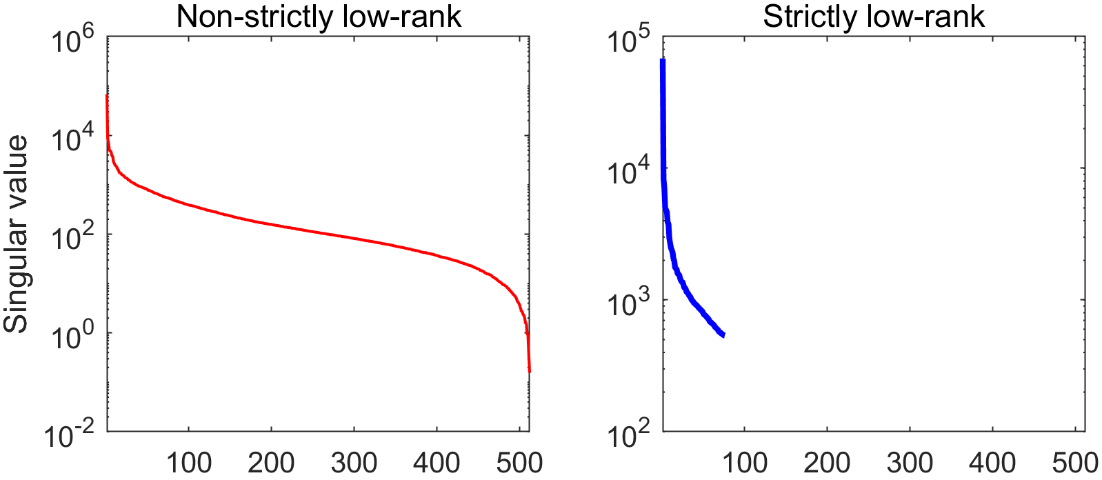
Figure 2: Sorted singular values in the two cases. Left: Non-strictly low-rank (the original image is used). Right: Strictly low-rank (the singular values of the original image are truncated to retain only the largest 15%).

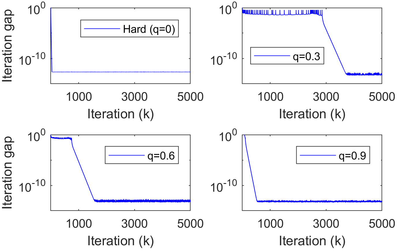
(a) Zero initialization

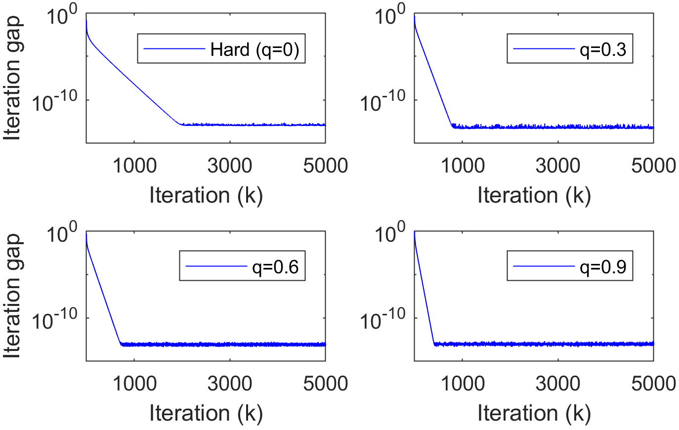
(b) Initialized with the solution of soft-thresholding

Figure 3: Convergence behavior of the PGD algorithm in the nonconvex case, (a) initialized with zero, (b) initialized with the solution of soft-thresholding.

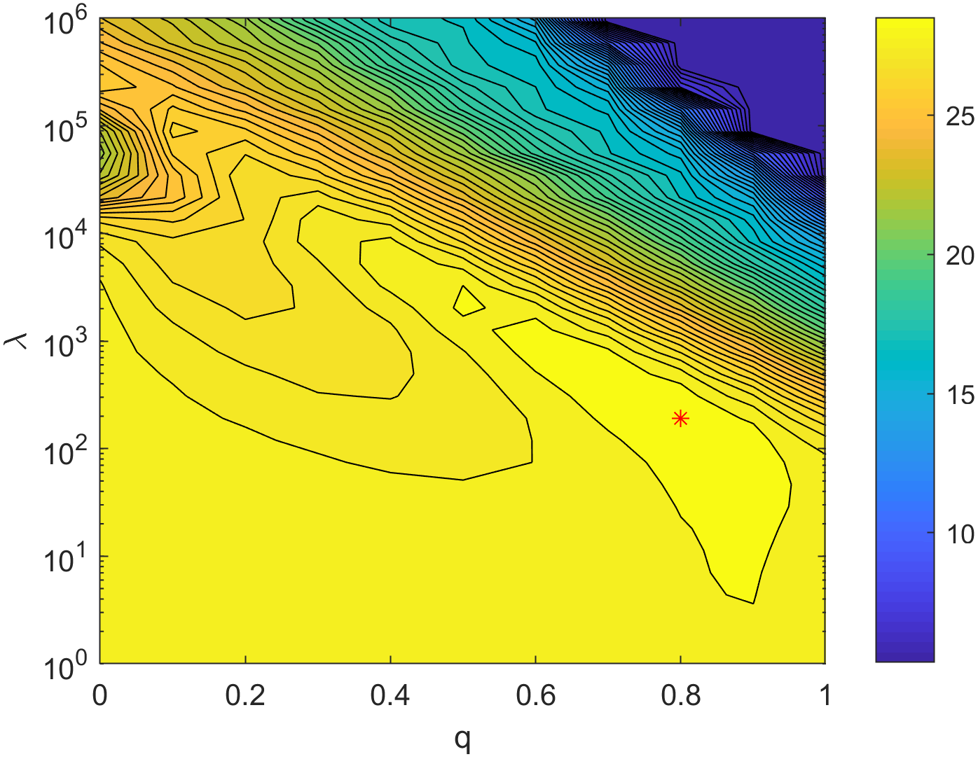
(a) Non-strictly low-rank

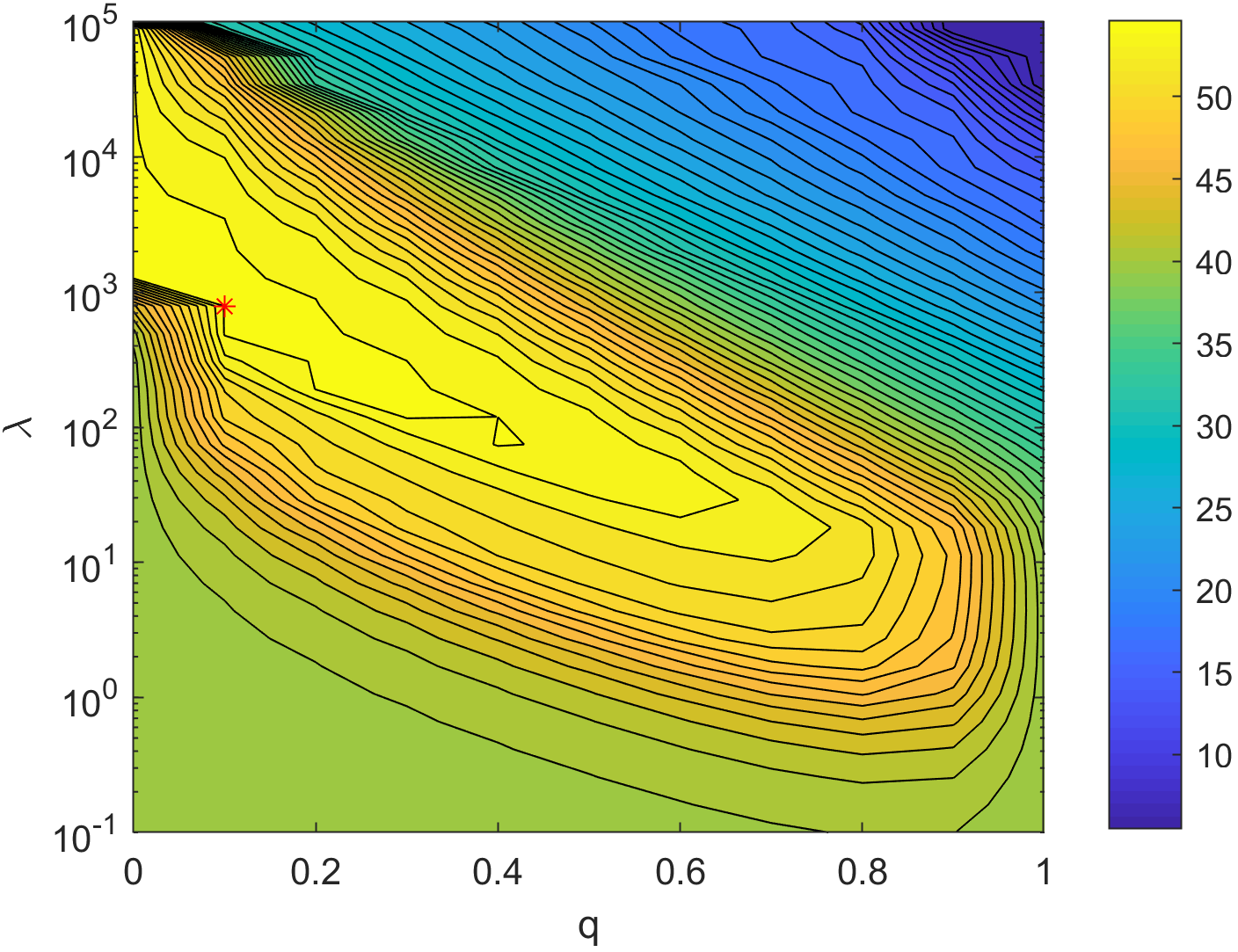
(b) Strictly low-rank

Figure 4: Recovery PSNR of the PGD algorithm with $\ell_{q}$ penalty in the case of SNR = 40 dB, (a) non-strictly low-rank, (b) strictly low-rank.

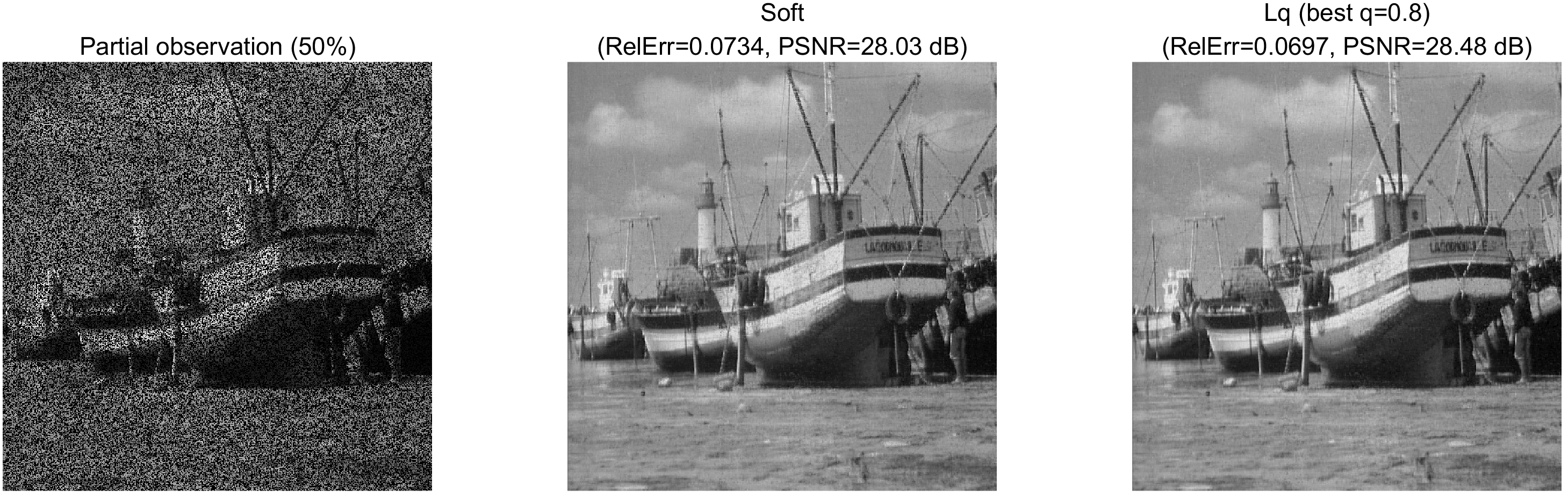
(a) Non-strictly low-rank

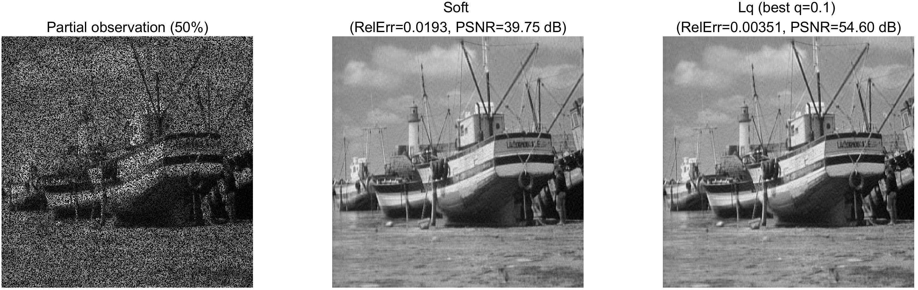
(b) Strictly low-rank

Figure 5: Recovery performance of the PGD algorithm on strictly and non-strictly low-rank images for SNR = 40 dB (along with the RelErr and PSNR of recovery). The values of $q$ providing the best performance of the $\ell_{q}$ penalty is presented.

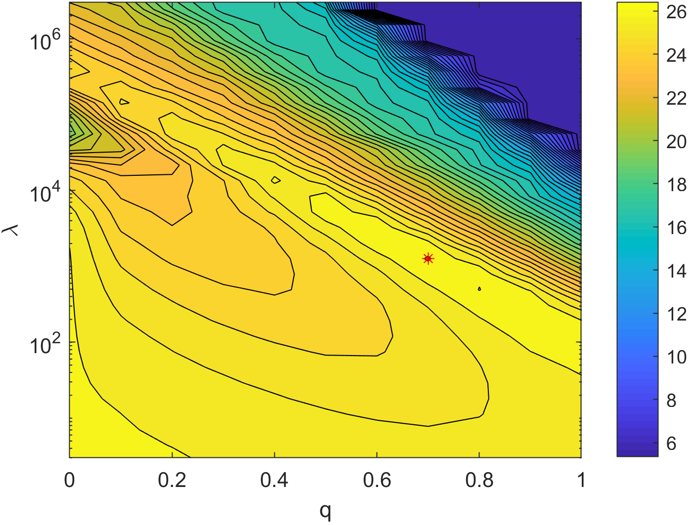
(a) Non-strictly low-rank

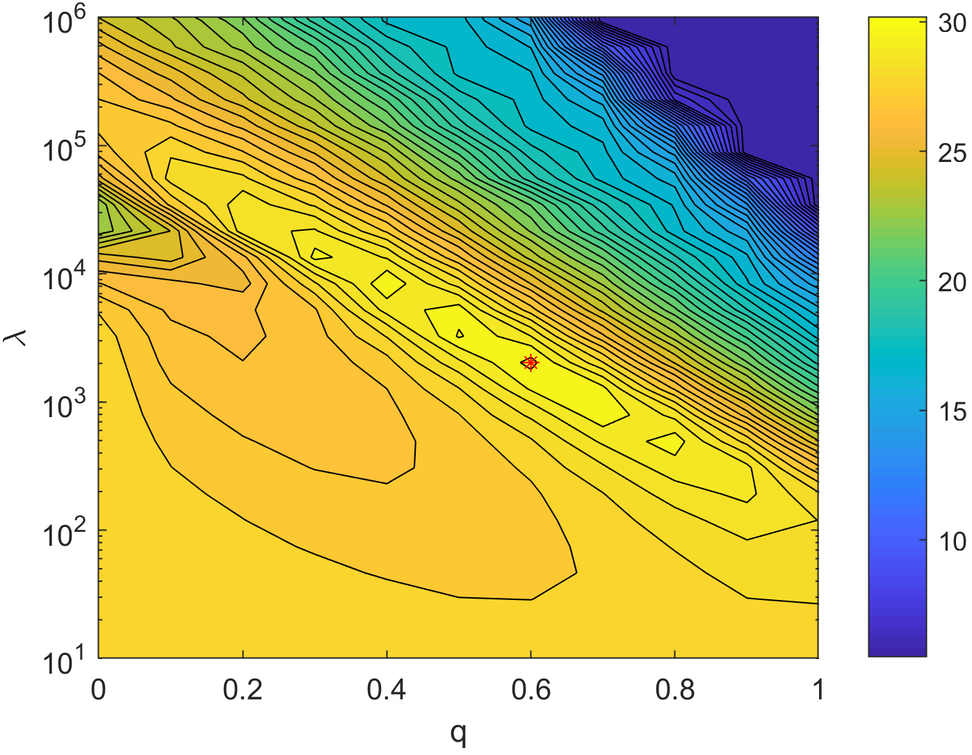
(b) Strictly low-rank

Figure 6: Recovery PSNR of the PGD algorithm with $\ell_{q}$ penalty in the case of SNR = 15 dB, (a) non-strictly low-rank, (b) strictly low-rank.

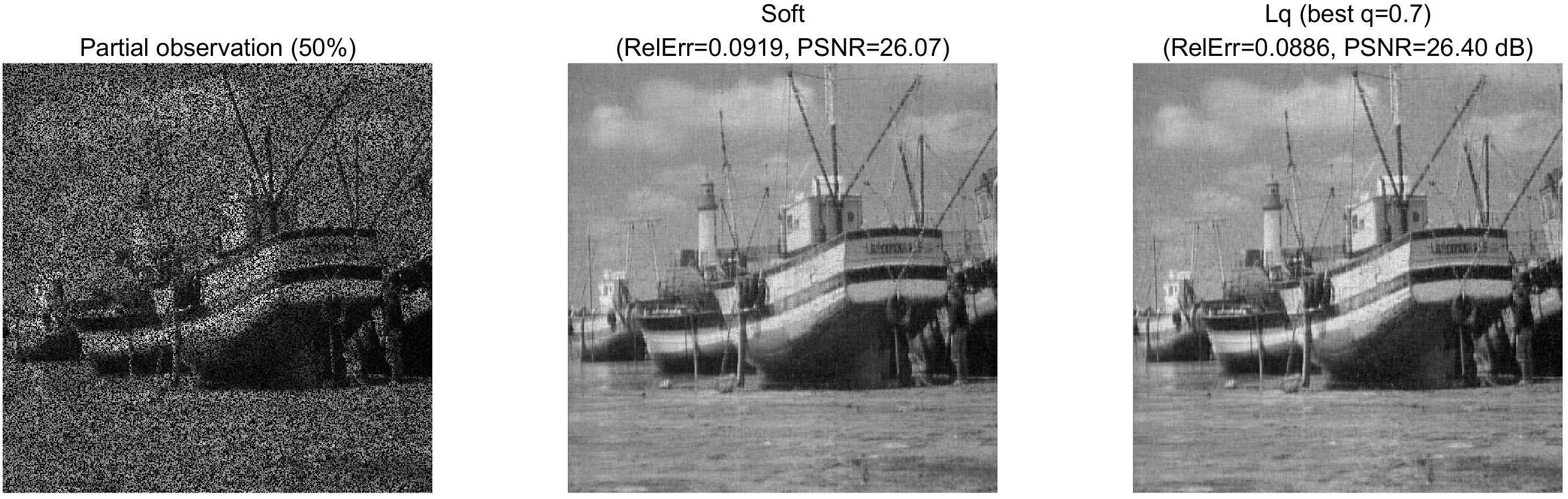
(a) Non-strictly low-rank

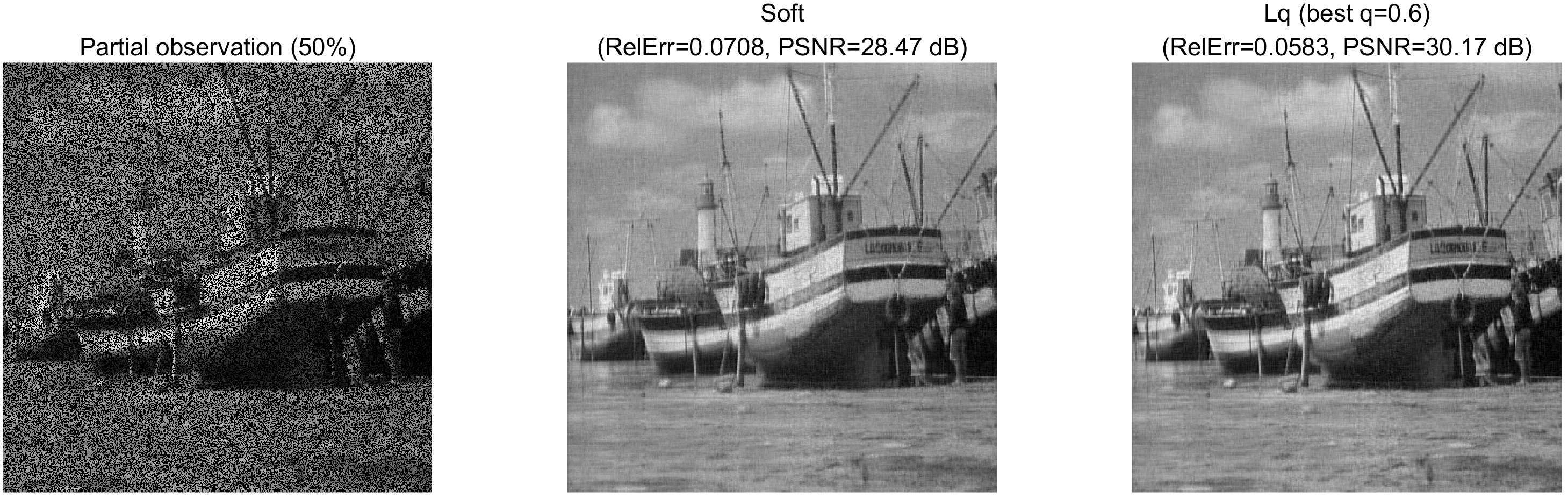
(b) Strictly low-rank

Figure 7: Recovery performance of the PGD algorithm on strictly and non-strictly low-rank images for SNR = 15 dB (along with the RelErr and PSNR of recovery). The values of $q$ providing the best performance of the $\ell_{q}$ penalty is presented.

In this section, we illustrate the PGD algorithm via numerical experiments on inpainting. We consider the $\ell_{q}$ penalty ($\bar{R}$ be the Schatten-$q$ norm) as it has a flexible parametric form that adapts to different penalty functions by varying the value of $q$. The goal is to recover a $512\times 512$ image from 50% of the pixels in the presence of entry noise, which is the case in many image inpainting and denoising applications (e.g., the other 50% of the pixels are corrupted by salt-and-pepper noise). Two cases are considered: 1) Non-strictly low-rank: the original image is used, which is not strictly low-rank but rather with singular values approximately following an exponential decay; 2) Strictly low-rank: the singular values of the original image are truncated and only the 15% largest values are retained, which results in a strictly low-rank image used for evaluation. Fig. 2 plots the sorted singular values in the two cases.

Fig. 3 shows the typical convergence behavior of the PGD algorithm for $q=\{0,0.3,0.6,0.9\}$ in two initialization conditions. The iteration gap ${\left\|{{{\bf{X}}^{k+1}}-{{\bf{X}}^{k}}}\right\|_{F}}/\sqrt{mn}$ is plotted. The results indicate that a good initialization facilitates the convergence of the PGD algorithm in the nonconvex case. Meanwhile, with zero initialization, the hard-thresholding seems to converge to a near local minimizer quickly. Eventually linear convergence rate of the PGD algorithm with $\ell_{q}$ penalty can be observed from the iteration gap variation. As well as most nonconvex algorithms, the performance of the PGD algorithm is closely related to the initialization. In the following, for the nonconvex case of $0\leq q<1$, we first run the PGD algorithm with $\ell_{1}$ (nuclear norm) penalty to obtain an initialization.

Fig. 4 shows the recovery peak-signal noise ratio (PSNR) of the PGD algorithm for different combinations of $q$ and $\lambda$ in the two considered cases, with entry-wise Gaussian noise of 40 dB. Fig. 5 shows the recovered images along with the relative error of recovery (RelErr) and PSNR of each recovered image. Fig. 6 and Fig. 7 show the results for a higher noise condition with entry-wise noise of 15 dB. The recovery PSNR comparison between the $\ell_{q}$ and $\ell_{1}$ penalties is provided in Table II. It can be seen that with a properly selected value of $q$, the $\ell_{q}$ penalty outperforms the $\ell_{1}$ penalty in all cases. The advantage of the $\ell_{q}$ penalty over the $\ell_{1}$ penalty is more prominent in the strictly low-rank case. For example in the low noise case with SNR = 40 dB, the advantage in the strictly low-rank case is about 14.85 dB, while that in the non-strictly low-rank case is only about 0.45 dB. This advantage wakens in the high noise case with SNR = 15 dB.

TABLE II: Recovery PSNR comparison (in dB) (along with the values of $q$ providing the best performance of the $\ell_{q}$ penalty).

	SNR = 40 dB		SNR = 15 dB
	$\ell_{1}$	$\ell_{q}$	$\ell_{1}$	$\ell_{q}$
non-strictly low-rank	28.03	28.48 ($q=0.8$)	26.07	26.40 ($q=0.7$)
strictly low-rank	39.75	54.60 ($q=0.1$)	28.47	30.17 ($q=0.6$)

Moreover, the results imply that for the $\ell_{q}$ penalty, in the low noise condition, e.g., SNR = 40 dB, a relatively small value of $q$, e.g., $q<0.5$, should be used in the strictly low-rank case, while a relatively large value of $q$, e.g., $q>0.5$, should be used in the non-strictly low-rank case. However, in the high noise case, e.g., SNR = 15 dB, a moderate value of $q$ tends to yield good performance.

V Conclusion

This work provided an analysis on the PGD algorithm for matrix completion using a nonconvex penalty. First, some properties on the gradient and Hessian of a generalized low-rank penalty have been established. Then, we provide more deep analysis on a popular class of nonconvex penalties which have discontinuous thresholding functions. For such penalties, we established the finite rank change, convergence to a restricted strictly local minimizer and an eventually linear convergence rate for the PGD algorithm under certain conditions. Meanwhile, convergence to a local minimizer has been obtained for the PGD algorithm with hard-thresholding penalty. Experimental results on inpainting demonstrated that, the benefit of using a nonconvex penalty is especially conspicuous in recovering a strictly low-rank matrix in the presence of small noise.

Appendix A Gradient and Hessian of Functions Contains Low-rank Penalty

In general, a low-rank penalty function is not differential with respective to a low-rank matrix. For example, for a generalized low-rank penalty defined as (8), $\bar{R}({\bf{X}})=R({\bm{\sigma}}({\bf{X}}))$ for a matrix ${\bf{X}}\in{\mathbb{R}^{m\times n}}$, since $R$ is usually nonsmooth at zero (such as the penalties mentioned in section II), $R({\bm{\sigma}}({\bf{X}}))$ is not differential when ${\rm{rank}}({\bf{X}})<\min(m,n)$. However, when $R$ is $C^{2}$ on $(0,+\infty)$, it is differential on $C^{2}$ arcs $t\to{\bf{X}}(t)$ if ${\rm{rank}}({\bf{X}}(t))$ is constant, although the rank may be less than $\min(m,n)$). Consider the latter case, we can analytically derive the gradient and Hessian of a function which contains a low-rank penalty as a term.

Suppose that ${\bf{X}}$ is of rank $r$, $r\leq\min(m,n)$, with any truncated SVD ${\bf{X}}={\bf{U\Sigma V}}^{T}$, where ${\bf{\Sigma}}={\bf{diag}}({{\bm{\sigma}}_{r}}({\bf{X}}))$, ${\bf{U}}\in{\mathbb{R}^{m\times r}}$ and ${\bf{V}}\in{\mathbb{R}^{m\times r}}$ contains the corresponding singular vectors. When $R$ is $C^{2}$ on $(0,+\infty)$ with first- and second-order derivative be $R^{\prime}$ and $R^{\prime\prime}$, respectively, denote

$${\bf{\Sigma^{\prime}}}={\bf{diag}}(R^{\prime}({\sigma_{1}}({\bf{X}})),\cdots,R^{\prime}({\sigma_{r}}({\bf{X}})))$$

$${\bf{\Sigma^{\prime\prime}}}={\bf{diag}}(R^{\prime\prime}({\sigma_{1}}({\bf{X}})),\cdots,R^{\prime\prime}({\sigma_{r}}({\bf{X}}))).$$

The differential of ${\bf{X}}$ can be computed as

$${\rm{d}}{\bf{X}}={\rm{d}}{\bf{U\Sigma}}{{\bf{V}}^{T}}+{\bf{U}}{\rm{d}}{\bf{\Sigma}}{{\bf{V}}^{T}}{\rm{+}}{\bf{U\Sigma}}{\rm{d}}{{\bf{V}}^{T}}.$$ (26)

Meanwhile, with ${{\bf{U}}^{T}}{\bf{U}}={{\bf{V}}^{T}}{\bf{V}}={{\bf{I}}_{r}}$ and

$${{\bf{U}}^{T}}{\rm{d}}{\bf{U\Sigma}}+{\bf{\Sigma}}{\rm{d}}{{\bf{V}}^{T}}{\bf{V}}={\bf{0}}$$ (27)

it follows that

$${{\bf{U}}^{T}}{\rm{d}}{\bf{XV}}={{\bf{U}}^{T}}{\rm{d}}{\bf{U\Sigma}}+{\rm{d}}{\bf{\Sigma}}+{\bf{\Sigma}}{\rm{d}}{{\bf{V}}^{T}}{\bf{V}}={\rm{d}}{\bf{\Sigma}}.$$ (28)

Then, we have

$${\rm{d}}R({{\bm{\sigma}}_{r}}({\bf{X}}))={\rm{d}}({\rm{tr(}}R({\bf{\Sigma}}){\rm{))}}={\rm{tr(}}{\bf{\Sigma^{\prime}}}{\rm{d}}{\bf{\Sigma}}{\rm{)}}={\rm{tr(}}{\bf{V\Sigma^{\prime}}}{{\bf{U}}^{T}}{\rm{d}}{\bf{X}}{\rm{)}}.$$ (29)

Thus, the gradient of $R({{\bm{\sigma}}_{r}}({\bf{X}}))$ is given by

$${\nabla_{\bf{X}}}R({{\bm{\sigma}}_{r}}({\bf{X}}))={\bf{U\Sigma^{\prime}}}{{\bf{V}}^{T}}.$$

A-A Derivation of (12)

Using (26)–(29)), the differential of the objective $T$ with respect to ${\bf{X}}$ can be expressed as

$$\begin{split}&{\rm{d}}(T({\bf{X}}))\\ &={\rm{d}}({\rm{tr(}}R({\bf{\Sigma}}){\rm{))}}+\frac{\eta}{2}{\rm{d}}\left({{\rm{tr(}}{{\bf{\Sigma}}^{2}}{\rm{)}}-{\rm{2tr}}({{\bf{T}}^{T}}{\bf{U\Sigma}}{{\bf{V}}^{T}})}\right)\\ &={\rm{tr(}}{\bf{V\Sigma^{\prime}}}{{\bf{U}}^{T}}{\rm{d}}{\bf{X}}{\rm{)}}+\eta\left({{\rm{tr(}}{\bf{\Sigma}}{\rm{d}}{\bf{\Sigma}}{\rm{)}}-{\rm{tr}}({{\bf{T}}^{T}}{\bf{U}}{\rm{d}}{\bf{\Sigma}}{{\bf{V}}^{T}})}\right)\\ &={\rm{tr(}}{\bf{V\Sigma^{\prime}}}{{\bf{U}}^{T}}{\rm{d}}{\bf{X}}{\rm{)}}+\eta{\rm{tr(}}{\bf{V\Sigma}}{{\bf{U}}^{T}}{\rm{d}}{\bf{X}}{\rm{)}}-\\ &~{}~{}~{}~{}~{}~{}~{}~{}~{}~{}~{}~{}~{}~{}~{}~{}~{}~{}~{}~{}~{}~{}~{}~{}~{}~{}~{}~{}~{}~{}\eta{\rm{tr}}({\bf{V}}{{\bf{V}}^{T}}{{\bf{T}}^{T}}{\bf{U}}{{\bf{U}}^{T}}{\rm{d}}{\bf{X}}).\end{split}$$ (30)

Thus, we have

$${\nabla_{\bf{X}}}T({\bf{X}})={{\bf{U}}^{T}}{\bf{\Sigma^{\prime}V}}+\eta\left({{\bf{X}}+{\bf{U}}{{\bf{U}}^{T}}{\bf{TV}}{{\bf{V}}^{T}}}\right)$$

which results in (12).

A-B Hessian of $R({{\bm{\sigma}}_{r}}({\bf{X}}))$

Follows from (29), using (26) we have

$$\begin{split}&{{\rm{d}}^{2}}R({{\bm{\sigma}}_{r}}({\bf{X}}))\\ &={\rm{tr}}\left({\left[{{\rm{d}}{\bf{V\Sigma^{\prime}}}{{\bf{U}}^{T}}+{\bf{V\Sigma^{\prime\prime}}}{\rm{d}}{\bf{\Sigma}}{{\bf{U}}^{T}}+{\bf{V\Sigma^{\prime}}}{\rm{d}}{{\bf{U}}^{T}}}\right]{\rm{d}}{\bf{X}}}\right)\\ &={\rm{tr}}\left({{\bf{V\Sigma^{\prime\prime}}}{\rm{d}}{\bf{\Sigma}}{{\bf{U}}^{T}}{\rm{d}}{\bf{X}}}\right)+{\rm{tr}}\left({{\rm{d}}{{\bf{X}}^{T}}({\rm{d}}{\bf{U\Sigma^{\prime}}}{{\bf{V}}^{T}}{\rm{+}}{\bf{U\Sigma^{\prime}}}{\rm{d}}{{\bf{V}}^{T}})}\right).\end{split}$$ (31)

Next, we show that

$${\rm{tr}}\left({{\rm{d}}{{\bf{X}}^{T}}({\rm{d}}{\bf{U\Sigma^{\prime}}}{{\bf{V}}^{T}}{\rm{+}}{\bf{U\Sigma^{\prime}}}{\rm{d}}{{\bf{V}}^{T}})}\right)={\bf{0}}.$$ (32)

There exists a full SVD ${\bf{X}}{\rm{=}}\bar{\bf{U}}\bar{\bf{\Sigma}}{\bar{\bf{V}}^{T}}$, with $\bar{\bf{U}}\in{\mathbb{R}^{m\times m}}$, $\bar{\bf{V}}\in{\mathbb{R}^{n\times n}}$ and $\bar{\bf{\Sigma}}\in{\mathbb{R}^{m\times n}}$, such that

$${\bf{U}}=\bar{\bf{U}}(:,1:r),~{}~{}{\bf{V}}=\bar{\bf{V}}(:,1:r),~{}~{}\bar{\bf{\Sigma}}=\left[{\begin{array}[]{*{20}{c}}\!{\bf{\Sigma}}&{\bf{0}}\!\\ \!{\bf{0}}&{\bf{0}}\!\end{array}}\right].$$

Then, denote

$$\bar{\bf{\Sigma}}^{\prime}=\left[{\begin{array}[]{*{20}{c}}\!{{\bf{\Sigma^{\prime}}}}&{\bf{0}}\!\\ \!{\bf{0}}&{\bf{0}}\!\end{array}}\right]$$

and use ${\bar{\bf{V}}^{T}}\bar{\bf{V}}=\bar{\bf{V}}{\bar{\bf{V}}^{T}}={{\bf{I}}_{n}}$, ${\bar{\bf{U}}^{T}}\bar{\bf{U}}{\rm{=}}\bar{\bf{U}}{\bar{\bf{U}}^{T}}{\rm{=}}{{\bf{I}}_{m}}$, ${\bar{\bf{U}}^{T}}{\rm{d}}\bar{\bf{U}}\bar{\bf{\Sigma}}^{\prime}{\rm{+}}\bar{\bf{\Sigma}}^{\prime}{\rm{d}}{\bar{\bf{V}}^{T}}\bar{\bf{V}}={\bf{0}}$, (32) can be justified as

$${\rm{tr}}\left({{\rm{d}}{{\bf{X}}^{T}}\left({{\rm{d}}{\bf{U\Sigma^{\prime}}}{{\bf{V}}^{T}}{\rm{+}}{\bf{U\Sigma^{\prime}}}{\rm{d}}{{\bf{V}}^{T}}}\right)}\right)$$

$$={\rm{tr}}\left({{\rm{d}}{{\bf{X}}^{T}}\left({{\rm{d}}\bar{\bf{U}}\bar{\bf{\Sigma}}^{\prime}{{\bar{\bf{V}}}^{T}}{\rm{+}}\bar{\bf{U}}\bar{\bf{\Sigma}}^{\prime}{\rm{d}}{{\bar{\bf{V}}}^{T}}}\right)}\right)$$

$$={\rm{tr}}\left({{\rm{d}}{{\bf{X}}^{T}}\bar{\bf{U}}{{\bar{\bf{U}}}^{T}}\left({{\rm{d}}\bar{\bf{U}}\bar{\bf{\Sigma}}^{\prime}{{{\bf{\bar{V}}}}^{T}}{\rm{+}}\bar{\bf{U}}\bar{\bf{\Sigma}}^{\prime}{\rm{d}}{{\bar{\bf{V}}}^{T}}}\right)\bar{\bf{V}}{{\bar{\bf{V}}}^{T}}}\right)$$

$$={\rm{tr}}\left({{\rm{d}}{{\bf{X}}^{T}}\bar{\bf{U}}\left({{{\bar{\bf{U}}}^{T}}{\rm{d}}\bar{\bf{U}}\bar{\bf{\Sigma}}^{\prime}{\rm{+}}\bar{\bf{\Sigma^{\prime}}}{\rm{d}}{{\bar{\bf{V}}}^{T}}\bar{\bf{V}}}\right){{\bar{\bf{V}}}^{T}}}\right)$$

$$={\bf{0}}.$$

Substituting (32) into (31), and using (28) and ${\rm{tr}}({\bf{ABCD}})={\rm{ve}}{{\rm{c}}^{T}}({{\bf{B}}^{T}})({{\bf{A}}^{T}}\otimes{\bf{C}}){\rm{vec}}({\bf{D}})$ yield

$$\begin{split}&{{\rm{d}}^{2}}R({{\bm{\sigma}}_{r}}({\bf{X}}))={\rm{tr}}\left({{\bf{V\Sigma^{\prime\prime}}}{{\bf{U}}^{T}}{\rm{d}}{\bf{XV}}{{\bf{U}}^{T}}{\rm{d}}{\bf{X}}}\right)\\ &={[{\rm{d(vec(}}{\bf{X}}{\rm{))]}}^{T}}{{\bf{K}}_{nm}}[({\bf{U\Sigma^{\prime\prime}}}{{\bf{V}}^{T}})\otimes({\bf{V}}{{\bf{U}}^{T}})]{\rm{d(vec(}}{\bf{X}}{\rm{))}}\end{split}$$ (33)

where ${{\bf{K}}_{nm}}$ is a commutation matrix defined as ${\rm{vec}}({\bf{A}})={{\bf{K}}_{nm}}{\rm{vec}}({{\bf{A}}^{T}})$ for ${\bf{A}}\in{\mathbb{R}^{m\times n}}$. Then, follows from (33) and the relation between Hessian matrix and second-order differential [51], Lemma 2 is derived.

Appendix B Proof of Lemma 3

First, using $({\bf{AB}})\otimes({\bf{CD}})=({\bf{A}}\otimes{\bf{C}})({\bf{B}}\otimes{\bf{D}})$, we have

$$({\bf{U\Sigma^{\prime\prime}}}{{\bf{V}}^{T}})\otimes({\bf{V}}{{\bf{U}}^{T}})+({\bf{U}}{{\bf{V}}^{T}})\otimes({\bf{V\Sigma^{\prime\prime}}}{{\bf{U}}^{T}})$$

$$=({\bf{U}}\otimes{\bf{V}})({\bf{\Sigma^{\prime\prime}}}\otimes{{\bf{I}}_{r}}){({\bf{V}}\otimes{\bf{U}})^{T}}$$

$$~{}~{}+({\bf{U}}\otimes{\bf{V}})({{\bf{I}}_{r}}\otimes{\bf{\Sigma^{\prime\prime}}}){({\bf{V}}\otimes{\bf{U}})^{T}}$$

$$=({\bf{U}}\otimes{\bf{V}})({\bf{\Sigma^{\prime\prime}}}\otimes{{\bf{I}}_{r}}+{{\bf{I}}_{r}}\otimes{\bf{\Sigma^{\prime\prime}}}){({\bf{V}}\otimes{\bf{U}})^{T}}.$$

Then, with the properties of commutation matrix,

$${{\bf{K}}_{nm}}({\bf{U}}\otimes{\bf{V}}){{\bf{K}}_{rr}}={\bf{V}}\otimes{\bf{U}}$$

and ${{\bf{K}}_{rr}}{\bf{K}}_{rr}^{-1}={{\bf{K}}_{rr}}{{\bf{K}}_{rr}}={{\bf{I}}_{{r^{2}}}}$, it follows that

$$\nabla_{\bf{X}}^{2}R({{\bm{\sigma}}_{r}}({\bf{X}}))$$

$$=\frac{1}{2}{{\bf{K}}_{nm}}\big{[}{({\bf{U}}\otimes{\bf{V}})({\bf{\Sigma^{\prime\prime}}}\otimes{{\bf{I}}_{r}}+{{\bf{I}}_{r}}\otimes{\bf{\Sigma^{\prime\prime}}}){{({\bf{V}}\otimes{\bf{U}})}^{T}}}\big{]}$$

$$=\frac{1}{2}({\bf{V}}\otimes{\bf{U}})\left[{{{\bf{K}}_{rr}}({\bf{\Sigma^{\prime\prime}}}\otimes{{\bf{I}}_{r}}+{{\bf{I}}_{r}}\otimes{\bf{\Sigma^{\prime\prime}}})}\right]{({\bf{V}}\otimes{\bf{U}})^{T}}.$$

Since ${{\bf{V}}^{T}}{\bf{V}}={{\bf{U}}^{T}}{\bf{U}}={{\bf{I}}_{r}}$, it is easy to see that

$${({\bf{V}}\otimes{\bf{U}})^{T}}({\bf{V}}\otimes{\bf{U}})=({{\bf{V}}^{T}}{\bf{V}}\otimes{{\bf{U}}^{T}}{\bf{U}})={{\bf{I}}_{{r^{2}}}}$$

which implies the columns of the matrix $({\bf{V}}\otimes{\bf{U}})$ are orthogonal. Meanwhile, the commutation matrix ${{\bf{K}}_{rr}}$ is orthogonal and in fact ${{\bf{K}}_{rr}}({\bf{\Sigma^{\prime\prime}}}\otimes{{\bf{I}}_{r}}+{{\bf{I}}_{r}}\otimes{\bf{\Sigma^{\prime\prime}}})$ is a rearrange of the diagonal elements of the diagonal matrix $({\bf{\Sigma^{\prime\prime}}}\otimes{{\bf{I}}_{r}}+{{\bf{I}}_{r}}\otimes{\bf{\Sigma^{\prime\prime}}})$. Thus, when $R^{\prime\prime}\neq 0$ on $(0,\infty)$, it follows from ${{\bm{\sigma}}_{r}}({\bf{X}})>0$ that

$${\rm{rank}}\left({\nabla_{\bf{X}}^{2}R({{\bm{\sigma}}_{r}}({\bf{X}}))}\right)={r^{2}}$$

and the $r^{2}$ nonzero eigenvalues of $\nabla_{\bf{X}}^{2}R({{\bm{\sigma}}_{r}}({\bf{X}}))$ are given by

$${\bm{\lambda}}\left({\nabla_{\bf{X}}^{2}R({{\bm{\sigma}}_{r}}({\bf{X}}))}\right)={\bm{\lambda}}({\bf{\Sigma^{\prime\prime}}}\otimes{{\bf{I}}_{r}}+{{\bf{I}}_{r}}\otimes{\bf{\Sigma^{\prime\prime}}}).$$

Moreover, under the assumption that $R^{\prime\prime}$ is a nondecreasing function on $(0,\infty)$, and with ${\sigma_{r}}({\bf{X}})=\min({{\bm{\sigma}}_{r}}({\bf{X}}))$, we have

$${\lambda_{\min}}\left({\nabla_{\bf{X}}^{2}R({{\bm{\sigma}}_{r}}({\bf{X}}))}\right)=R^{\prime\prime}({\sigma_{r}}({\bf{X}}))$$

$${\rm{and}}~{}~{}~{}~{}~{}~{}~{}~{}~{}~{}{\lambda_{\max}}\left({\nabla_{\bf{X}}^{2}R({{\bm{\sigma}}_{r}}({\bf{X}}))}\right)=0~{}~{}~{}~{}~{}~{}~{}~{}~{}~{}~{}~{}~{}~{}~{}~{}~{}~{}~{}~{}~{}~{}~{}~{}~{}~{}~{}~{}$$

which concludes the proof.

Appendix C Proof of Lemma 4

Let ${\beta_{L}}$ be the larger output of the singular value thresholding function ${P_{R,L/\lambda}}$ (corresponding to ${\bar{P}_{\bar{R},L/\lambda}}$ in (16)) at its discontinuous point. That is, ${\beta_{L}}$ is the jumping size at the discontinuous point of ${P_{R,L/\lambda}}$. Then, for any ${{\bf{X}}^{k}}$ generated by the PGD algorithm, it follows from the discontinuous thresholding property that, for $1\leq i\leq\min(m,n),~{}\forall k>0$,

$$\begin{split}{\sigma_{i}}({{\bf{X}}^{k}})\geq{\beta_{L}},&~{}~{}~{}{\rm{if}}~{}~{}~{}{\sigma_{i}}({{\bf{X}}^{k}})\neq 0.\end{split}$$ (34)

By Property 2(ii), there exists a sufficiently large positive integer ${k_{0}}$ such that when $k>{k_{0}}$ it holds

$${\left\|{{{\bf{X}}^{k+1}}-{{\bf{X}}^{k}}}\right\|_{F}}<{\beta_{L}}$$

which together with Lemma 1 implies

$${\left\|{{\bm{\sigma}}({{\bf{X}}^{k+1}})-{\bm{\sigma}}({{\bf{X}}^{k}})}\right\|_{2}}<{\beta_{L}}.$$ (35)

Denote ${r^{k}}={\rm{rank}}({{\bf{X}}^{k}})$, it follows from (34) that

$${\left\|{{\bm{\sigma}}({{\bf{X}}^{k+1}})-{\bm{\sigma}}({{\bf{X}}^{k}})}\right\|_{2}}\geq{\beta_{L}},~{}~{}{\rm{if}}~{}~{}{r^{k+1}}\neq{r^{k}}$$

which contradicts to (35) when $k>{k_{0}}$. Thus, ${r^{k+1}}={r^{k}}$ when $k>{k_{0}}$. It means that the rank of ${{\bf{X}}^{k}}$ converges

$${r^{k+1}}={r^{k}}=r,~{}~{}\forall k>{k_{0}}.$$ (36)

For any cluster point ${{\bf{X}}^{*}}$, there exists a subsequence $\{{{\bf{X}}^{{k_{j}}}}\}$ converging to ${{\bf{X}}^{*}}$, i.e., ${{\bf{X}}^{{k_{j}}}}\to{{\bf{X}}^{*}}$ as $j\to\infty$. Thus, there exists a sufficiently large positive integer ${j_{0}}$ such that ${k_{{j_{0}}}}>{k_{0}}$ and

$${\left\|{{\bm{\sigma}}({{\bf{X}}^{{k_{j}}}})-{\bm{\sigma}}({{\bf{X}}^{*}})}\right\|_{2}}<{\beta_{L}}$$

when $j>{j_{0}}$. Similar to the above analysis, we have

$${r^{{k_{j}}}}={\rm{rank(}}{{\bf{X}}^{*}}{\rm{)}},~{}~{}~{}~{}\forall j>{j_{0}}.$$

From (36), ${r^{{k_{j}}}}=r$, thus ${\rm{rank(}}{{\bf{X}}^{*}}{\rm{)}}=r$ for any cluster point ${{\bf{X}}^{*}}$. Consequently, taking ${k^{*}}>{k_{{j_{0}}}}$, Lemma 4 is proved based on the above analysis.

Appendix D Proof of Theorem 1

The condition in Theorem 1 implies that

$$\nabla_{\bf{X}}^{2}\bar{F}({{\bf{X}}^{*}})=\lambda\nabla_{\bf{X}}^{2}R({{\bm{\sigma}}_{r}}({{\bf{X}}^{*}}))+{\bf{diag}}({\rm{vec}}({{\bf{{\bf P}}}_{\Omega}}))\succeq{\bf{0}}.$$ (37)

Consider a sufficiently small matrix ${\bf{E}}$ with ${\left\|{\bf{E}}\right\|_{F}}<{\beta_{L}}$, ${\beta_{L}}$ is the is the “jumping” size of the singular value thresholding function ${P_{R,L/\lambda}}$ (corresponding to ${\bar{P}_{\bar{R},L/\lambda}}$ in (16)) at the its discontinuous point. Under Assumption 2, we have $\min\left({{{\bm{\sigma}}_{r}}({{\bf{X}}^{*}})}\right)\geq{\beta_{L}}$, thus, ${\rm{rank}}({{\bf{X}}^{*}}+{\bf{E}})\geq r$ for such a small ${\bf{E}}$. This can be justified as follows. With ${\left\|{\bf{E}}\right\|_{F}}<{\beta_{L}}$, by Lemma 1

$${\left\|{{{\bm{\sigma}}_{r}}({{\bf{X}}^{*}})-{{\bm{\sigma}}_{r}}({{\bf{X}}^{*}}+{\bf{E}})}\right\|_{2}}<{\beta_{L}}.$$ (38)

Since $\min\left({{{\bm{\sigma}}_{r}}({{\bf{X}}^{*}})}\right)\geq{\beta_{L}}$, it follows that

$${\left\|{{{\bm{\sigma}}_{r}}({{\bf{X}}^{*}})-{{\bm{\sigma}}_{r}}({{\bf{X}}^{*}}+{\bf{E}})}\right\|_{2}}\geq{\beta_{L}}~{}~{}{\rm{if}}~{}~{}{\rm{rank}}({{\bf{X}}^{*}}+{\bf{E}})<r$$

which contradict to (38).

Let $\tilde{\bf{U}}{\bf{diag}}\left({{\bm{\sigma}}({{\bf{X}}^{*}}+{\bf{E}})}\right){\tilde{\bf{V}}^{T}}$ be any full SVD of $({{\bf{X}}^{*}}+{\bf{E}})$ and denote

$${\bf{X}}_{e}^{*}=\tilde{\bf{U}}{\bf{diag}}\left({[{\bm{\sigma}}_{r}^{T}({{\bf{X}}^{*}}+{\bf{E}}),{\bf{0}}]}\right){\tilde{\bf{V}}^{T}}$$

$${\bf{X}}_{e\bot}^{*}=\tilde{\bf{U}}{\bf{diag}}\left({[{\bf{0}},{\bm{\sigma}}_{r\bot}^{T}({{\bf{X}}^{*}}+{\bf{E}})]}\right){\tilde{\bf{V}}^{T}}.$$

From the property of stationary point, ${{\bf{X}}^{*}}$ satisfies

$${\nabla_{\bf{X}}}G({{\bf{X}}^{*}})+\lambda{\nabla_{\bf{X}}}R({{\bm{\sigma}}_{r}}({{\bf{X}}^{*}}))={\bf{0}}.$$ (39)

Then, it follows from (37) and (39) that for sufficiently small matrix ${\bf{E}}$,

$$\begin{split}&G({\bf{X}}_{e}^{*})+\lambda R({{\bm{\sigma}}_{r}}({{\bf{X}}^{*}}+{\bf{E}}))\\ &\geq G({{\bf{X}}^{*}})+\lambda R({{\bm{\sigma}}_{r}}({{\bf{X}}^{*}}))=F({{\bf{X}}^{*}}).\end{split}$$ (40)

Denote

$${\bf{y}}={\rm{diag}}\left({{{\tilde{\bf{V}}}^{T}}{{[{\nabla_{{\bf{X}}_{e\bot}^{*}}}f({\bf{X}}_{e}^{*})]}^{T}}\tilde{\bf{U}}}\right).$$

For sufficiently small ${\bf{E}}$, by Lemma 1 and ${\rm{rank}}({{\bf{X}}^{*}})=r$, ${\sigma_{i}}({{\bf{X}}^{*}}+{\bf{E}})$ is also sufficiently small for $r+1\leq i\leq\min(m,n)$, then under Assumption 1 it holds that for $r+1\leq i\leq\min(m,n)$,

$$R({\sigma_{i}}({{\bf{X}}^{*}}+{\bf{E}}))\geq\frac{{{{\left\|{\bf{y}}\right\|}_{\infty}}}}{\lambda}{\sigma_{i}}({{\bf{X}}^{*}}+{\bf{E}})$$

where the equality holds if and only if ${\sigma_{i}}({{\bf{X}}^{*}}+{\bf{E}})=0$. Thus, for a sufficiently small ${\bf{E}}$ (hence ${\sigma_{i}}({{\bf{X}}^{*}}+{\bf{E}})$ is sufficient small for $r+1\leq i\leq\min(m,n)$), using ${{\bf{X}}^{*}}+{\bf{E}}={\bf{X}}_{e}^{*}+{\bf{X}}_{e\bot}^{*}$ and ${\bf{X}}_{e\bot}^{*}$ be also sufficient small, it holds that

$$\begin{split}&G({{\bf{X}}^{*}}+{\bf{E}})-G({\bf{X}}_{e}^{*})+\lambda R({{\bm{\sigma}}_{r\bot}}({{\bf{X}}^{*}}+{\bf{E}}))\\ &=\left\langle{{\nabla_{{\bf{X}}_{e\bot}^{*}}}G({\bf{X}}_{e}^{*}),{\bf{X}}_{e\bot}^{*}}\right\rangle+\lambda R({{\bm{\sigma}}_{r\bot}}({{\bf{X}}^{*}}+{\bf{E}}))+o\left({{{\left\|{{\bf{X}}_{e\bot}^{*}}\right\|}_{F}}}\right)\\ &={\rm{tr}}\left({{{[{\nabla_{{\bf{X}}_{e\bot}^{*}}}G({\bf{X}}_{e}^{*})]}^{T}}\tilde{\bf{U}}{\bf{diag}}\left({[{\bf{0}},{\bm{\sigma}}_{r\bot}^{T}({{\bf{X}}^{*}}+{\bf{E}})]}\right){{\tilde{\bf{V}}}^{T}}}\right)\\ &~{}~{}~{}~{}~{}~{}~{}~{}~{}~{}+\lambda R({{\bm{\sigma}}_{r\bot}}({{\bf{X}}^{*}}+{\bf{E}}))+o\left({{{\left\|{{\bm{\sigma}}_{r\bot}^{T}({{\bf{X}}^{*}}+{\bf{E}})}\right\|}_{2}}}\right)\\ &=\sum\limits_{i=r+1}^{\min(m,n)}{[{\bf{y}}(i){\sigma_{i}}({{\bf{X}}^{*}}+{\bf{E}})+\lambda R({\sigma_{i}}({{\bf{X}}^{*}}+{\bf{E}}))]}\\ &~{}~{}~{}~{}~{}~{}~{}~{}~{}~{}~{}~{}~{}~{}~{}~{}~{}+o\left({{{\left\|{{\bm{\sigma}}_{r\bot}^{T}({{\bf{X}}^{*}}+{\bf{E}})}\right\|}_{2}}}\right)\\ &\geq 0.\end{split}$$ (41)

Then, summing up the two inequalities (40) and (41), we have

$$F({{\bf{X}}^{*}}+{\bf{E}})-F({{\bf{X}}^{*}})\geq 0$$

for sufficiently small ${\bf{E}}$, which implies that ${{\bf{X}}^{*}}$ is a local minimizer of $F$.

Appendix E Proof of Theorem 2

The derivation follows similar to that in Appendix D. Briefly, the condition in Theorem 2 implies that

$$\nabla_{{{\bf{X}}_{\Omega}}}^{2}\bar{F}({{\bf{X}}^{*}})=\lambda\nabla_{{{\bf{X}}_{\Omega}}}^{2}R({{\bm{\sigma}}_{r}}({{\bf{X}}^{*}}))+{{\bf{I}}_{|\Omega|}}\succ{\bf{0}}.$$ (42)

Consider a sufficiently small matrix ${\bf{E}}$ with ${\left\|{\bf{E}}\right\|_{F}}<{\beta_{L}}$ such that ${\rm{rank}}({{\bf{X}}^{*}}+{\mathcal{P}_{\Omega}}({\bf{E}}))\geq r$ under Assumption 2. Let $\tilde{\bf{U}}{\bf{diag}}\left({{\bm{\sigma}}({{\bf{X}}^{*}}+{\mathcal{P}_{\Omega}}({\bf{E}}))}\right){\tilde{\bf{V}}^{T}}$ be any full SVD of $({{\bf{X}}^{*}}+{\mathcal{P}_{\Omega}}({\bf{E}}))$ and denote

$${\bf{X}}_{e}^{*}=\tilde{\bf{U}}{\bf{diag}}\left({[{\bm{\sigma}}_{r}^{T}({{\bf{X}}^{*}}+{\mathcal{P}_{\Omega}}({\bf{E}})),{\bf{0}}]}\right){\tilde{\bf{V}}^{T}}$$

$${\bf{X}}_{e\bot}^{*}=\tilde{\bf{U}}{\bf{diag}}\left({[{\bf{0}},{\bm{\sigma}}_{r\bot}^{T}({{\bf{X}}^{*}}+{\mathcal{P}_{\Omega}}({\bf{E}}))]}\right){\tilde{\bf{V}}^{T}}.$$

From the property of stationary point, ${{\bf{X}}^{*}}$ satisfies

$${\nabla_{{{\bf{X}}_{\Omega}}}}G({{\bf{X}}^{*}})+\lambda{\nabla_{{{\bf{X}}_{\Omega}}}}R({{\bm{\sigma}}_{r}}({{\bf{X}}^{*}}))={\bf{0}}.$$ (43)

Then, it follows from (42) and (43) that for sufficiently small matrix ${\bf{E}}$,

$$\begin{split}&G({\bf{X}}_{e}^{*})+\lambda R({{\bm{\sigma}}_{r}}({{\bf{X}}^{*}}+{\mathcal{P}_{\Omega}}({\bf{E}})))\\ &>G({{\bf{X}}^{*}})+\lambda R({{\bm{\sigma}}_{r}}({{\bf{X}}^{*}}))=F({{\bf{X}}^{*}}).\end{split}$$ (44)

For sufficiently small ${\bf{E}}$, ${\sigma_{i}}({{\bf{X}}^{*}}+{\bf{E}})$ is also sufficiently small for $r+1\leq i\leq\min(m,n)$, then, similar to (41) we have

$$G({{\bf{X}}^{*}}+{\mathcal{P}_{\Omega}}({\bf{E}}))-G({\bf{X}}_{e}^{*})+\lambda R({{\bm{\sigma}}_{r\bot}}({{\bf{X}}^{*}}+{\mathcal{P}_{\Omega}}({\bf{E}})))\geq 0.$$ (45)

Then, summing up (44) and (45), it follows that for sufficiently small ${\bf{E}}$,

$$F({{\bf{X}}^{*}}+{\mathcal{P}_{\Omega}}({\bf{E}}))-F({{\bf{X}}^{*}})>0$$

which implies that ${{\bf{X}}^{*}}$ is a $\Omega$-restricted strictly local minimizer of $F$ by Definition 2.

Appendix F Proof of Theorem 3

From Lemma 4, for $\delta<{\beta_{L}}$, there exists a sufficiently large integer ${k^{0}}>{k^{*}}$ (${k^{*}}$ defined in Lemma 4) such that ${\left\|{{{\bf{X}}^{k}}-{{\bf{X}}^{*}}}\right\|_{F}}<\delta$ and ${\rm{rank}}({{\bf{X}}^{k}})={r}$, $\forall k>{k^{0}}$. Let ${\bf{X}}$ be a rank-$r$ matrix with a truncated SVD ${\bf{X}}={\bf{Udiag}}\left({{{\bm{\sigma}}_{r}}({\bf{X}})}\right){{\bf{V}}^{T}}$, by Lemma 4, when $k>{k^{0}}$ the PGD algorithm in fact minimizes the following objective

$$f({\bf{X}}):=\lambda R({{\bm{\sigma}}_{r}}({\bf{X}}))+\frac{L}{2}\left\|{{\bf{X}}-{{\bf{X}}^{k}}+\frac{1}{L}\nabla G({{\bf{X}}^{k}})}\right\|_{F}^{2}$$

for which the gradient is (a similar derivation as in Appendix A)

$${\nabla_{\bf{X}}}f({\bf{X}})=\lambda{\nabla_{\bf{X}}}R({{\bm{\sigma}}_{{r}}}({\bf{X}}))+L({\bf{X}}-{\bf{U}}{{\bf{U}}^{T}}{{\bf{Q}}^{k}}{\bf{V}}{{\bf{V}}^{T}})$$ (46)

where ${{\bf{Q}}^{k}}={{\bf{X}}^{k}}-\frac{1}{L}\nabla G({{\bf{X}}^{k}})$. For $k>{k^{0}}$, let ${{\bf{X}}^{k}}={{\bf{U}}^{k}}{\bf{diag}}({{\bm{\sigma}}_{r}}({{\bf{X}}^{k}})){({{\bf{V}}^{k}})^{T}}$ and ${{\bf{X}}^{*}}={{\bf{U}}^{*}}{\bf{diag}}({{\bm{\sigma}}_{r}}({{\bf{X}}^{*}})){{\bf{V}}^{*}}^{T}$ be any truncated SVD of ${{\bf{X}}^{k}}$ and ${{\bf{X}}^{*}}$, respectively. For notation simplification in the sequel, we denote

$${\bm{\sigma}}_{r}^{k}={{\bm{\sigma}}_{r}}({{\bf{X}}^{k}}),~{}{\bm{\sigma}}_{r}^{*}={{\bm{\sigma}}_{r}}({{\bf{X}}^{*}}),~{}{{\bf{Q}}^{*}}={{\bf{X}}^{*}}-\frac{1}{L}\nabla G({{\bf{X}}^{*}}),$$

$${{\bf{\Sigma}}^{k+1}}={({{\bf{U}}^{k+1}})^{T}}{{\bf{Q}}^{k}}{{\bf{V}}^{k+1}},~{}~{}{{\bf{\Sigma}}^{*}}={{\bf{U}}^{*}}^{T}{{\bf{Q}}^{*}}{{\bf{V}}^{*}}.$$

From (46) the minimizer ${{\bf{X}}^{k+1}}$ satisfies ${\nabla_{\bf{X}}}f({{\bf{X}}^{k+1}})={\bf{0}}$, hence

$${{\bf{X}}^{k+1}}+\frac{\lambda}{L}{\nabla_{\bf{X}}}R({\bm{\sigma}}_{r}^{k+1})={{\bf{U}}^{k+1}}{{\bf{\Sigma}}^{k+1}}{({{\bf{V}}^{k+1}})^{T}}.$$ (47)

Meanwhile,

$${{\bf{X}}^{*}}+\frac{\lambda}{L}{\nabla_{\bf{X}}}R({\bf{\sigma}}_{r}^{*})={{\bf{U}}^{*}}{{\bf{\Sigma}}^{*}}{({{\bf{V}}^{*}})^{T}}.$$ (48)

Then, it follows from (47) and (48) that

$$\begin{split}&{{\bf{X}}^{k+1}}-{{\bf{X}}^{*}}+\frac{\lambda}{L}[{\nabla_{\bf{X}}}R({\bm{\sigma}}_{r}^{k+1})-{\nabla_{\bf{X}}}R({\bm{\sigma}}_{r}^{*})]\\ &={{\bf{U}}^{k+1}}{{\bf{\Sigma}}^{k+1}}{({{\bf{V}}^{k+1}})^{T}}-{{\bf{U}}^{*}}{{\bf{\Sigma}}^{*}}{{\bf{V}}^{*}}^{T}.\end{split}$$ (49)

By (24)

$$\begin{split}&\Big{\langle}{{{\bf{X}}^{k+1}}\!-\!{{\bf{X}}^{*}}\!+\!\frac{\lambda}{L}[{\nabla_{\bf{X}}}R({\bm{\sigma}}_{{r}}^{k+1})\!-\!{\nabla_{\bf{X}}}R({\bm{\sigma}}_{{r}}^{*})],{{\bf{X}}^{k+1}}-{{\bf{X}}^{*}}}\Big{\rangle}\\ &\geq(1+\lambda R^{\prime\prime}(\sigma)/L-\lambda{c_{R}}/L)\left\|{{{\bf{X}}^{k+1}}-{{\bf{X}}^{*}}}\right\|_{F}^{2}.\end{split}$$ (50)

From Property 1, ${{\bf{U}}^{k+1}}$ and ${{\bf{V}}^{k+1}}$ are the singular vectors of ${{\bf{Q}}^{k}}$ corresponding to ${{\bm{\sigma}}_{r}}({{\bf{Q}}^{k}})$, and

$${{\bf{\Sigma}}^{k+1}}={({{\bf{U}}^{k+1}})^{T}}{{\bf{Q}}^{k}}{{\bf{V}}^{k+1}}={\bf{diag}}({{\bm{\sigma}}_{r}}({{\bf{Q}}^{k}})).$$

Meanwhile, ${{\bf{U}}^{*}}$ and ${{\bf{V}}^{*}}$ are the singular vectors of ${{\bf{Q}}^{*}}$ corresponding to ${{\bm{\sigma}}_{r}}({{\bf{Q}}^{*}})$, and

$${{\bf{\Sigma}}^{*}}={{\bf{U}}^{*}}^{T}{{\bf{Q}}^{*}}{{\bf{V}}^{*}}={\bf{diag}}({{\bm{\sigma}}_{r}}({{\bf{Q}}^{*}})).$$

Then, it follows from (25) and Assumption 3 that, in a sufficiently small neighborhood of ${{\bf{X}}^{*}}$, there exists constants ${\alpha^{k}}:=\alpha({{\bf{X}}^{k}})$ (which is sufficiently small), ${\gamma^{k}}:=\gamma({{\bf{X}}^{k}})\in[0,1)$ and ${\xi^{k}}:=\xi({{\bf{X}}^{k}})\in(0,1)$, satisfying ${\beta^{k}}:=1/(1+2{\alpha^{k}})-{\gamma^{k}}>0$, such that

$$\begin{split}&\left\|{{{\bf{U}}^{k+1}}{{\bf{\Sigma}}^{k+1}}{{({{\bf{V}}^{k+1}})}^{T}}-{{\bf{U}}^{*}}{{\bf{\Sigma}}^{*}}{{\bf{V}}^{*}}^{T}}\right\|_{F}^{2}\\ &={\beta^{k}}\left\|{{{\bf{Q}}^{k}}-{{\bf{Q}}^{*}}}\right\|_{F}^{2}\\ &\!=\!{\beta^{k}}\left\|{\Big{(}1\!-\!\frac{1}{L}\Big{)}\left[{{\mathcal{P}}_{\Omega}}({{\bf{X}}^{k}})\!-\!{{\mathcal{P}}_{\Omega}}({{\bf{X}}^{*}})\right]\!+\!{\mathcal{P}}_{\Omega}^{\bot}({{\bf{X}}^{k}})\!-\!{\mathcal{P}}_{\Omega}^{\bot}({{\bf{X}}^{*}})}\right\|_{F}^{2}\\ &={\beta^{k}}\left\|{\Big{(}1-\frac{1}{L}\Big{)}{{\mathcal{P}}_{\Omega}}({{\bf{X}}^{k}}-{{\bf{X}}^{*}})+{\mathcal{P}}_{\Omega}^{\bot}({{\bf{X}}^{k}}-{{\bf{X}}^{*}})}\right\|_{F}^{2}\\ &={\beta^{k}}\left[{{{\Big{(}1-\frac{1}{L}\Big{)}}^{2}}\left\|{{{\mathcal{P}}_{\Omega}}({{\bf{X}}^{k}}-{{\bf{X}}^{*}})}\right\|_{F}^{2}+\left\|{{\mathcal{P}}_{\Omega}^{\bot}({{\bf{X}}^{k}}-{{\bf{X}}^{*}})}\right\|_{F}^{2}}\right]\\ &={\beta^{k}}\Big{(}1-\frac{2{\xi^{k}}}{L}+\frac{\xi^{k}}{L^{2}}\Big{)}\left\|{{{\bf{X}}^{k}}-{{\bf{X}}^{*}}}\right\|_{F}^{2}\end{split}$$ (51)

where $0<1-\frac{2{\xi^{k}}}{L}+\frac{\xi^{k}}{L^{2}}<1$ since $0<{\xi^{k}}<1$ and $L>1$. Then, it follows that

$$\begin{split}&\big{\langle}{{{\bf{U}}^{k+1}}{{\bf{\Sigma}}^{k+1}}{{({{\bf{V}}^{k+1}})}^{T}}-{{\bf{U}}^{*}}{{\bf{\Sigma}}^{*}}{{\bf{V}}^{*}}^{T},{{\bf{X}}^{k+1}}-{{\bf{X}}^{*}}}\big{\rangle}\\ &\leq{\left\|{{{\bf{U}}^{k+1}}{{\bf{\Sigma}}^{k+1}}{{({{\bf{V}}^{k+1}})}^{T}}-{{\bf{U}}^{*}}{{\bf{\Sigma}}^{*}}{{\bf{V}}^{*}}^{T}}\right\|_{F}}{\left\|{{{\bf{X}}^{k+1}}-{{\bf{X}}^{*}}}\right\|_{F}}\\ &\leq\sqrt{{\beta^{k}}\Big{(}1-\frac{2\xi^{k}}{L}+\frac{\xi^{k}}{L^{2}}\Big{)}}{\left\|{{{\bf{X}}^{k}}-{{\bf{X}}^{*}}}\right\|_{F}}{\left\|{{{\bf{X}}^{k+1}}-{{\bf{X}}^{*}}}\right\|_{F}}.\end{split}$$ (52)

Under the conditions in Theorem 2, we have $1+\lambda R^{\prime\prime}(\sigma)/L>0$ since $1+\lambda R^{\prime\prime}(\sigma)>0$ and $L>1$, which implies

$$1+\lambda R^{\prime\prime}(\sigma)/L-\lambda{c_{R}}/L>0$$

for sufficiently small ${c_{R}}$. In this case, from (49), (50) and (52), and without loss of any generality assuming that ${\left\|{{{\bf{X}}^{k+1}}-{{\bf{X}}^{*}}}\right\|_{F}}>0$ (the condition before convergence), we have

$${\left\|{{{\bf{X}}^{k+1}}-{{\bf{X}}^{*}}}\right\|_{F}}\leq\frac{{\sqrt{{\beta^{k}}(1-2{\xi^{k}}{\rm{/}}L+{\xi^{k}}{\rm{/}}{L^{2}})}}}{{1+\lambda R^{\prime\prime}(\sigma)/L-\lambda{c_{R}}/L}}{\left\|{{{\bf{X}}^{k}}-{{\bf{X}}^{*}}}\right\|_{F}}.$$ (53)

Let

$${\rho^{k}}=\frac{{\sqrt{{\beta^{k}}(1-2{\xi^{k}}{\rm{/}}L+{\xi^{k}}{\rm{/}}{L^{2}})}}}{{1+\lambda R^{\prime\prime}(\sigma)/L-\lambda{c_{R}}/L}}.$$

Consider a sufficiently small neighborhood of ${\bf{X}}^{*}$ with sufficiently small $\delta$, thus ${c_{R}}$ and ${\alpha^{k}}$ are sufficiently small, and with $0\leq{\gamma^{k}}<1$ and $0<{\xi^{k}}<1$, it holds $0<{\rho^{k}}<1$ if

$$1+\lambda R^{\prime\prime}(\sigma)/L>\sqrt{(1-{\gamma^{k}})(1-2{\xi^{k}}{\rm{/}}L+{\xi^{k}}{\rm{/}}{L^{2}})}.$$

When ${\gamma^{k}}$ and ${\xi^{k}}$ are respectively lower bounded by some $\gamma\in[0,1)$ and $\xi\in(0,1)$, $\forall k>{k^{0}}$, ${\rho^{k}}$ is upper bounded by some $\rho\in(0,1)$ if

$$1+\lambda R^{\prime\prime}(\sigma)/L>\sqrt{(1-\gamma)(1-2\xi{\rm{/}}L+\xi{\rm{/}}{L^{2}})}.$$ (54)

Thus, Theorem 3 is proved.

References

• [1] E. J. CandΓ¨s and B. Recht, β€œExact matrix completion via convex optimization,” Found. Comput. Math., vol. 9, no. 6, pp. 717–772, 2009.
• [2] E. J. CandΓ¨s and T. Tao, β€œThe power of convex relaxation: Near-optimal matrix completion,” IEEE Trans. Inf. Theory, vol. 56, no. 5, pp. 2053–2080, May 2010.
• [3] B. Recht, β€œA simpler approach to matrix completion,” J. Mach. Learn. Res., vol. 12, pp. 3413–3430, Jan. 2011.
• [4] P. D. M. Geona, M. Baburaj, and S. N. George, β€œEntropy-based reweighted tensor completion technique for video recovery,” IEEE Trans. Circuits and Systems for Video Technology, 2019.
• [5] R. Sun and Z. Q. Luo, β€œGuaranteed matrix completion via non-convex factorization,” IEEE Trans. Inf. Theory, vol. 62, no. 11, pp. 6535–6579, 2016.
• [6] F. Cao, M. Cai, and Y. Tan, β€œImage interpolation via low-rank matrix completion and recovery,” IEEE Trans. Circuits and Systems for Video Technology, vol. 25, no. 8, pp. 1261–1270, 2015.
• [7] R. Mazumder, T. Hastie, and R. Tibshirani, β€œSpectral regularization algorithms for learning large incomplete matrices,” J. Mach. Learn. Res., vol. 11, pp. 2287–2322, 2010.
• [8] J. Abernethy, F. Bach, T. Evgeniou, and J. P. Vert, β€œA new approach to collaborative filtering: Operator estimation with spectral regularization,” JMLR, vol. 10, pp. 803–826, 2009.
• [9] F. Wen, P. Liu. Y. Liu, R. C. Qiu, W. Yu, β€œRobust sparse recovery in impulsive noise via Lp-L1 optimization,” IEEE Trans. Signal Processing, vol. 65, no. 1, pp. 105–118, Jan. 2017.
• [10] N. Komodakis and G. Tziritas, β€œImage completion using global optimization,” in Proc. IEEE Conf. Computer Vision and Pattern Recognition, 2006.
• [11] T. Zhao, Z. Wang, and H. Liu, β€œA nonconvex optimization framework for low rank matrix estimation,” in Advances in Neural Information Processing Systems, pp. 559–567, 2015.
• [12] H. Ji, C. Liu, Z. Shen, and Y. Xu, β€œRobust video denoising using low rank matrix completion,” in Proc. IEEE Conf. Computer Vision and Pattern Recognition, 2010.
• [13] P. Chen and D. Suter, β€œRecovering the missing components in a large noisy low-rank matrix: Application to SFM,” IEEE Trans. Pattern Anal. Mach. Intell., vol. 26, no. 8, pp. 1051–1063, Aug. 2004.
• [14] Z. Liu and L. Vandenberghe, β€œInterior-point method for nuclear norm approximation with application to system identification,” SIAM J. Matrix Anal. Appl., vol. 31, no. 3, pp. 1235–1256, 2009.
• [15] A. Argyriou, C. A. Micchelli, and M. Pontil, β€œConvex multi-task feature learning,” J. Mach. Learn., vol. 73, no. 3, pp. 243–272, 2006.
• [16] G. Obozinski, B. Taskar, and M. Jordan, β€œJoint covariate selection and joint subspace selection for multiple classification problems,” Stat. Comput., vol. 20, pp. 231–252, 2010.
• [17] K. Q. Weinberger and L. K. Saul, β€œUnsupervised learning of image manifolds by semidefinite programming,” Int. J. Comput. Vis., vol. 70, pp. 77–90, 2006.
• [18] R. Ge, J. D. Lee, and T. Ma, β€œMatrix completion has no spurious local minimum,” in Advances in Neural Information Processing Systems, pp. 2973–2981, 2016.
• [19] S. Ma, D. Goldfarb, and L. Chen, β€œFixed point and Bregman iterative methods for matrix rank minimization,” Math. Program., vol. 128, no. 1–2, pp. 321–353, 2011.
• [20] K. C. Toh and S. Yun, β€œAn accelerated proximal gradient algorithm for nuclear norm regularized linear least squares problems,” Pacific J. Optim., vol. 6, no. 15, pp. 615–640, 2010.
• [21] E. J. CandΓ¨s and Y. Plan, β€œMatrix completion with noise,” Proc. IEEE, vol. 98, no. 6, pp. 925–936, Jun. 2010.
• [22] S. Negahban and M. J. Wainwright, β€œRestricted strong convexity and weighted matrix completion: Optimal bounds with noise,” J. Mach. Learn. Res., vol. 13, no. 1, pp. 1665–1697, 2012.
• [23] R. Chartrand and V. Staneva, β€œRestricted isometry properties and nonconvex compressive sensing,” Inverse Problems, vol. 24, no. 3, 2008.
• [24] F. Wen, L. Pei, Y. Yang, W. Yu, and P. Liu, β€œEfficient and robust recovery of sparse signal and image using generalized nonconvex regularization,” IEEE Trans. Computational Imaging, vol. 3, no. 4, pp. 566–579, 2017.
• [25] T. Hastie, R. Tibshirani, M. Wainwright. Statistical learning with sparsity: the lasso and generalizations. CRC Press, 2016.
• [26] F. Wen, L. Chu, P. Liu, and R. Qiu, β€œA survey on nonconvex regularization based sparse and low-rank recovery in signal processing, statistics, and machine learning,” IEEE Access, vol. 6, Nov. 2018.
• [27] G. Marjanovic and V. Solo, β€œOn $\ell_{q}$ optimization and matrix completion,” IEEE Trans. Signal Process., vol. 60, no. 11, pp. 5714–5724, 2012.
• [28] G. Marjanovic and V. Solo, β€œLq matrix completion,” ICASSP, 2012, pp. 3885–3888.
• [29] M. J. Lai, Y. Xu, and W. Yin, β€œImproved iteratively reweighted least squares for unconstrained smoothed Lq minimization,” SIAM J. Numer. Anal., vol. 51, no. 2, pp. 927–957, 2013.
• [30] Z. Lu and Y. Zhang, β€œSchatten-p quasi-norm regularized matrix optimization via iterative reweighted singular value minimization,” arXiv Preprint, arXiv:1401.0869v2, 2015.
• [31] Z. F. Jin, Z. Wan, Y. Jiao, et al., β€œAn alternating direction method with continuation for nonconvex low rank minimization,” Journal of Scientific Computing, vol. 66, no. 2, pp. 849–869, 2016.
• [32] F. Nie, H. Huang, and C. H. Q. Ding, β€œLow-rank matrix recovery via efficient Schatten p-norm minimization,” AAAI, 2012.
• [33] Y. Hu, D. Zhang, J. Ye, et al., β€œFast and accurate matrix completion via truncated nuclear norm regularization,” IEEE Trans. Pattern Analysis Machine Intelligence, vol. 35, no. 9, pp. 2117–2130, 2013.
• [34] F. Nie, H. Wang, X. Cai, et al., β€œRobust matrix completion via joint schatten p-norm and lp-norm minimization,” ICDM, 2012, pp. 566–574.
• [35] M. Malek-Mohammadi, M. Babaie-Zadeh, and M. Skoglund, β€œPerformance guarantees for Schatten-p quasi-norm minimization in recovery of low-rank matrices,” Signal Processing, vol. 114, pp. 225–230, 2015.
• [36] H. Attouch, J. Bolte, P. Redont, and A. Soubeyran, β€œProximal alternating minimization and projection methods for nonconvex problems: an approach based on the Kurdyka-Lojasiewicz inequality,” Mathematics of Operations Research, vol. 35, no. 2, pp. 438–457, 2010.
• [37] H. Attouch, J. Bolte, and B. Svaiter, β€œConvergence of descent methods for semi-algebraic and tame problems: Proximal algorithms, forward-backward splitting, and regularized Gauss-Seidel methods,” Math. Program. A, vol. 137, pp. 91–129, 2013.
• [38] G. Li and T. K. Pong, β€œGlobal convergence of splitting methods for nonconvex composite optimization,” SIAM J. Optimization, vol. 25, no. 4, pp. 2434–2460, Jul. 2015.
• [39] A. Agarwal, S. Negahban, and M. J. Wainwright, β€œFast global convergence of gradient methods for high-dimensional statistical recovery,” Ann. Statist., vol. 40, no. 5, pp. 2452–2482, 2012.
• [40] K. Hou, Z. Zhou, A. M.-C. So, and Z.-Q. Luo, β€œOn the linear convergence of the proximal gradient method for trace norm regularization,” in Proc. Adv. Neural Inf. Process. Syst. (NIPS), 2013, pp. 710–718.
• [41] R. Chartrand, β€œFast algorithms for nonconvex compressive sensing: MRI reconstruction from very few data,” in Proc. IEEE Int. Symp. Biomed. Imag., 2009, pp. 262–265.
• [42] J. Woodworth, R. Chartrand, β€œCompressed sensing recovery via nonconvex shrinkage penalties,” Inverse Problems, vol. 32, no. 7, pp. 1–25, 2016.
• [43] J. Fan and R. Li, β€œVariable selection via nonconcave penalized likelihood and its oracle properties,” Journal of the American Statistical Association, vol. 96, no. 456, pp. 1348–1360, 2001.
• [44] C. Zhang, β€œNearly unbiased variable selection under minimax concave penalty,” The Annals of Statistics, vol. 38, no. 2, pp. 894–942, 2010.
• [45] H.-Y. Gao and A. G. Bruce, β€œWave shrink with firm shrinkage,” Statistica Sinica, vol. 7, no. 4, pp. 855–874, 1997.
• [46] F. Wen, R. Ying, P. Liu, and T.-K. Truong, β€œNonconvex regularized robust PCA using the proximal block coordinate descent algorithm,” submitted to IEEE Trans. Signal Proessing.
• [47] A. J. Hoffman and H. W. Wielandt, β€œThe variation of the spectrum of a normal matrix,” Duke Math. J., vol. 20, no. 1, pp. 3–39, 1953.
• [48] J. Zeng, S. Lin, Y. Wang, and Z. Xu, β€œL1/2 regularization: Convergence of iterative half thresholding algorithm,” IEEE Trans. Signal Process., vol. 62, no. 9, pp. 2317–2329, Jul. 2014.
• [49] K. Bredies, D. Lorenz, and S. Reiterer, β€œMinimization of non-smooth, non-convex functionals by iterative thresholding,” J. Optim. Theory Appl., vol. 165, pp. 78–122, 2015.
• [50] J. Zeng, S. Lin, and Z. Xu, β€œSparse regularization: Convergence of iterative jumping thresholding algorithm,” IEEE Trans. Signal Process., vol. 64, no. 19, pp. 5106–5118, Oct. 2016.
• [51] J. R. Magnus and H. Neudecker, β€œMatrix differential calculus with applications in statistics and econometrics,” Wiley series in probability and mathematical statistics, 1988.