Nonparametric adaptive inference of birth and death models in a large population limit

Abstract.

Motivated by improving mortality tables from human demography databases, we investigate statistical inference of a stochastic age-evolving density of a population alimented by time inhomogeneous mortality and fertility. Asymptotics are taken as the size of the population grows within a limited time horizon: the observation gets closer to the solution of the Von Foerster Mc Kendrick equation, and the difficulty lies in controlling simultaneously the stochastic approximation to the limiting PDE in a suitable sense together with an appropriate parametrisation of the anisotropic solution. In this setting, we prove new concentration inequalities that enable us to implement the Goldenshluger-Lepski algorithm and derive oracle inequalities. We obtain minimax optimality and adaptation over a wide range of anisotropic Hölder smoothness classes.

Mathematics Subject Classification (2010): 62G05, 62M05, 60J80, 60J20, 92D25.

Keywords: Age-structured models, large population limit, concentration inequalities, nonparametric adaptive estimation, anisotropic estimation, Goldenshluger-Lepski method.

1. Introduction

1.1. Setting

Suppose one wishes to recover a probability density $g$ over the nonnegative real line $\mathbb{R}_{+}=[0,\infty)$ from a $N$-sample $a_{1},\ldots,a_{N}$, where the $a_{i}$ are not necessarily independent. If $Z^{N}=N^{-1}\sum_{i=1}^{N}\delta_{a_{i}}$ denotes the empirical distribution of the $N$-sample, designing a good statistical estimator of $g$ requires a fine quantitative control of the fluctuations in the convergence

(1) $$\int_{\mathbb{R}_{+}}\psi(a)Z^{N}(da)\rightarrow\int_{0}^{\infty}\psi(a)g(a)da$$

(at least in probability) as $N$ grows, for a large enough class of test functions $\psi$. Moreover, the performance of such a procedure depends on the smoothness properties of the function $g$, typically quantified by a smoothness parameter, like a (possibly fractional) number of derivatives in any reasonable sense and is usually unknown by the practitioner. For suitable $\psi$ (possibly data-dependent), optimal estimators can be found provided good concentration inequalities are available for (1), following the broad guiding principle of Lepski’s method [30, 17, 18] or other adaptive methods like model selection or wavelets, see for instance the comprehensive textbooks of Giné and Nickl [16] or Härdle et al. [19] or Tsybakov [44]. In this paper, we generalise the classical situation described above by adding a time variable. We investigate statistical inference of a time-evolving particle system governed by stochastic dynamics: for every $t\in[0,T]$, we observe the state of a population of (approximately) $N$ particles, encoded by its empirical measure $Z^{N}=\big{(}Z_{t}^{N}(da)\big{)}_{0\leq t\leq T}$. Informally, $Z^{N}$ is solution to a certain stochastic differential equation (SDE)

$$\mathcal{H}_{b,\mu}^{N}\big{(}Z^{N}\big{)}=0,$$

constructed in (10) below; $\mathcal{H}_{b,\mu}^{N}$ is parametrised by two functions $b$ and $\mu$ and $Z_{t}^{N}(da)$ represents the state of a population structured in age $a\in\mathbb{R}_{+}$, alimented by a time-inhomogeneous fertility rate $b(t,a)$ and decimated by a mortality rate $\mu(t,a)$. Moreover, we are given an initial empirical age distribution $Z_{0}^{N}$ at time $t=0$. Under appropriate regularity conditions we have a convergence $\mathcal{H}_{b,\mu}^{N}\rightarrow\mathcal{H}_{b,\mu}$ in a large population limit $N\rightarrow\infty$, where $\mathcal{H}_{b,\mu}(g)=0$ is an inhomogeneous version of the classical McKendrick Von Foerster renewal equation [35, 46], given by

(5) $$\left\{\begin{array}[]{ll}\partial_{t}g(t,a)+\partial_{a}g(t,a)+\mu(t,a)g(t,a)=0\\ \\ \displaystyle g(0,a)=g_{0}(a),\;\;g(t,0)=\int_{0}^{\infty}b(t,a)g(t,a)da.\\ \end{array}\right.$$

and that reveals the interplay between the limiting solution $g$ and the model parameter $b$ and $\mu$. In particular, we have a convergence

(6) $$\int_{0}^{T}\int_{\mathbb{R}_{+}}\psi(t,a)Z_{t}^{N}(da)dt\rightarrow\int_{0}^{T}\int_{0}^{\infty}\psi(t,a)g(t,a)da\,dt$$

(at least in probability) as $N$ grows for a rich enough class of functions $\psi$, and this situation generalises (1) in a time-dependent framework.

Informally, our statistical problem takes the following form: estimate $g$ or the parameters of the model $b,\mu$ from data $Z^{N}$ in the limit $N\rightarrow\infty$. In this setting, it is crucial to understand: (i) the quantitative properties of the convergence (6) and in particular, how concentration inequalities can be obtained (with a view towards an adaptive estimation scheme in the idea of Lepski’s principle) and (ii) what is the structure of the equation $\mathcal{H}_{b,\mu}(g)=0$ in terms of identification and interplay between the parameters $b,\mu,g$ and their smoothness properties. In particular, the anisotropic smoothness of $g$ viewed as a graph-manifold can benefit from the structure $\mathcal{H}_{b,\mu}(g)=0$ and lead to better approximation properties in certain directions along the characteristics of the transport.

1.2. Motivation

Of primary interest for us is human demography through the recent efforts and contributions for improving mortality estimates, see [8, 4, 5] among others and the references therein. In particular, the recent development of large human datasets like the Human Mortality Database (HMD) and Human Fertility Database (HFD) [21, 20] – in open access – allows one to process fertility and mortality data simultaneously, and subsequently addresses demographical issues such as the anomalies of cohort effects that have long fascinated demographers and actuaries [41, 7]. In this rejuvenated context, it becomes reasonable to study the estimation of population density or mortality rate in the enriched dynamical framework provided by birth-death particle systems that converge to the classical McKendrick Von Foerster equation in a large population limit, and revisit classical studies like e.g. [24, 38] for statistical estimation of the death rate; see the detailed literature review in next section. In this setting, we consider the idealised model where we can observe the (renormalised) evolution of the state of the population $Z^{N}_{t}$ continuously for $t\in[0,T]$, where $t=0$ is the starting date for the observation of the population and $t=T$ a terminal time horizon, fixed once for all. We are interested in identifying or estimating the parameters of the model. Of major importance is the inhomogeneous death rate $\mu(t,a)$. In our framework, we cannot recover the birth rate since we are not given any genealogical input: mathematically, this simply expresses the lack of injectivity of the mapping $b\mapsto g$. Still, our observation enables us to identify the functions $(t,a)\mapsto g(t,a)$ and $(t,a)\mapsto\mu(t,a)$ in the limit $N\rightarrow\infty$ and establish a thorough nonparametric estimation program, in the methodology of adaptive minimax estimation.

1.3. Link with literature on death rate inference

The main difficulty in establishing a consistent theory to estimate mortality rates comes from two key points: (i) incorporate the fact that the death rate depends on both age and time (non-homogeneous setting) and (ii) use as observables the outcome of a stochastic population dynamics (birth-death process). In the literature, we argue that each point is treated separately. The inference of a time-dependent death rate also related to a time-dependent covariate (possibly age), which relates to the first point has been addressed from a nonparametric perspective by e.g. [1, 12, 24, 34, 39, 6, 11] and the references therein. From [24], ”One way of understanding the difficulties in establishing an Aalen theory in the Lexis diagram is that although the diagram is two-dimensional, all movements are in the same direction (slope 1) and in the fully non-parametric model the diagram disintegrates into a continuum of life lines of slope 1 with freely varying intensities across lines. The cumulation trick from Aalen’s estimator (generalizing ordinary empirical distribution functions and Kaplan & Meier’s (1958) nonparametric empirical distribution function from censored data) does not help us here.” On the other side, the inference of an age-dependent death rate in an homogeneous birth-death model (or similar) - oiuyr second point - has been addressed in [9, 13, 22] among others. To the best of our knowledge, no statistical method deals with the usual problem faced by demographers related to the inference of a time and age-dependent death rate table based on the observation of population dynamics. Note that in this paper, the observation of the population is assumed to be continuous over time, whereas in practice the information on population exposure is extracted from census (point observation); these practical considerations are discussed in a companion paper, see [5].

1.4. Results and organisation of the paper

In a first part of the paper, Section 2, we construct the SDE that describes the state of the population $Z^{N}$ by means of a birth-death process characterised via a stochastic differential equation – given in (10) – driven by a random Poisson measure. We recall its convergence in a large population limit to the solution of the McKendrick Von Foerster equation $g$ based on classical results of [43, 36]. Our next step consists in quantifying the stability of the convergence $Z^{N}\rightarrow g$. To that end and anticipating the subsequent statistical analysis, we introduce two pseudo-distances:

$$\mathcal{W}_{w_{2}}^{N}(\mathcal{F})_{t}=\sup_{f\in\mathcal{F}}\int_{\mathbb{R}_{+}}w_{2}(t-a)f(t,a)\big{(}Z^{N}_{t}(da)-g(t,a)da\big{)}$$

and its integrated version

$$\mathcal{W}_{w_{1},w_{2}}^{N}(\mathcal{F})_{t}=\sup_{f\in\mathcal{F}}\int_{0}^{t}w_{1}(s)\int_{\mathbb{R}_{+}}w_{2}(s-a)f(s,a)\big{(}Z^{N}_{s}(da)-g(s,a)da\big{)}ds,$$

where $w_{1}$ and $w_{2}$ are two bounded weight functions and $\mathcal{F}$ a rich enough class of function with complexity measured in terms of entropy conditions. Note that formally $\mathcal{W}_{w_{2}}^{N}(\mathcal{F})_{t}$ is a degenerate version of $\mathcal{W}_{w_{1},w_{2}}^{N}(\mathcal{F})_{t}$. Taking $w_{1}=w_{2}=1$ is reminiscent of the 1-Wasserstein distance if $\mathcal{F}$ consists of $1$-Lipschitz functions. However, for the statistical analysis, we must be able to handle approximating kernels that do not have bounded Lipschitz norms, hence the presence of the weights $w_{1}$ and $w_{2}$ that can accomodate such kernels. The main result of this section, Theorem 6 states that under appropriate regularity conditions on $b$ and $\mu$, if $|w_{2}|_{1,\infty}^{-1}\mathcal{W}_{w_{2}}^{N}(\mathcal{F})_{0}$ is of (small) order $r_{N}$, so are

$$|w_{2}|_{1,\infty}^{-1}\mathcal{W}_{w_{2}}^{N}(\mathcal{F})_{T}\;\;\;\text{and}\;\;\;\big{(}|w_{1}|_{1,\infty}|w_{2}|_{1,\infty}\big{)}^{-1}\mathcal{W}_{\,w_{1},w_{2}}^{N}(\mathcal{F})_{T}.$$

The rate of decay $r_{N}$ possibly inflates by an order $N^{-1/2}$ and the result holds in terms of exponential decay of the fluctuation probabilities. The functional control $|\cdot|_{1,\infty}=(\|\cdot\|_{L^{1}}\|\cdot\|_{L^{\infty}})^{1/2}$ interpolates between $L^{1}$ and $L^{\infty}$-norms, and is sufficient to handle the behaviour of statistical kernels in an optimal way, since it can therefore be compared to the usual $L^{2}$-norm that appears in variance terms. The concentration of $\mathcal{W}_{w_{2}}^{N}(\mathcal{F})_{T}$ expresses a kind of stability of the particle system from $t=0$ to $t=T$, while the more intricate control of $\mathcal{W}_{\,w_{1},w_{2}}^{N}(\mathcal{F})_{T}$ is crucial to control variance terms in bi-variate kernel estimators for the nonparametric estimation of $g(t,a)$ and $\mu(t,a)$. The proof relies on a combination of martingales techniques in the spirit of Tran [43], a central reference for the paper, combined with classical tools from concentration of processes indexed by functions under entropy controls, following for instance Ledoux-Talagrand [28].

In a second part, Section 3, we construct nonparametric estimators of $g(t,a)$ and $\mu(t,a)$ by means of kernel approximation: we consider estimators of the form

$$\widehat{g}_{h}^{N}(t,a)=K_{h}\star Z_{t}^{N}(a)$$

for $g(t,a)$, where $\star$ denotes convolution and $K_{h}=h^{-1}K(h^{-1}\cdot)$, with $|K|_{1}=1$, is a kernel normalised in $L^{1}$ with bandwidth $h>0$. It is noteworthy that for estimating the population density $g(t,a)$ at time $t$, the information $Z_{t}^{N}$ is sufficient and we do not need the data $(Z_{s}^{N},s\neq t)$. The situation is very different for estimating $\mu(t,a)$ the main parameter of interest. We constuct a quotient estimator, inspired from a Nadaraya-Watson type procedure, and use

(7) $$\widehat{\mu}_{h_{1},h_{2},h_{3}}^{N}(t,a)=\frac{(H_{h_{1}}\otimes K_{h_{2}}\circ\varphi)\star\Gamma^{N}(du,ds)}{\widehat{g}_{h_{3}}^{N}(t,a)}$$

where $\Gamma^{N}(du,ds)$ is the point process of the death occurences in the population lifetime that can be extracted from $Z^{N}$ and that converges to $\pi=\mu g$, see (20) in Section 3.2 for the details. In (7), we consider a bivariate kernel $H\otimes K$ with bandwidth $(h_{1},h_{2})$ and $\varphi(t,a)=(t,t-a)$ is a certain change of coordinates that enables one to benefit from the smoothness along the characteristics of the transport. The choice of the bandwidths $h_{1},h_{2},h_{3}$ is chosen according to the data $Z^{N}$ itself, in the spirit of Lepski’s principle [17, 18]. In Theorems 11 and 13, we derive oracle inequalities that control the pointwise risk of $\widehat{g}_{h}^{N}(t,a)$ and $\widehat{\mu}_{h_{1},h_{2},h_{3}}^{N}(t,a)$ in terms of optimal balance between the error propagation of Theorem 6 and the linear approximation kernels.

Section 4 is devoted the adaptive estimation of $g$ and $\mu$ for the pointwise risk under smoothness constraints. In a first part, we study the smoothness of $g$ when $b$ and $\mu$ belong to anisotropic Hölder spaces (and for simplicity, we assume that the initial condition $g_{0}$ is sufficiently smooth). Thanks to the relatively explicit form of the solution of the McKendrick Von Foester equation, we establish in Proposition 16 that when parametrised via $\varphi$, the function $\widetilde{g}$ in the representation $g=\widetilde{g}\circ\varphi$ has explicitly quantifiable improved smoothness over $g$, suggesting to consider the approximation kernel $H_{h_{1}}\otimes K_{h_{2}}\circ\varphi$ for estimating $\pi$ via the quotient estimator (7) that implicitly uses the representation of $\mu=\pi/g$. We establish in Theorem 18 minimax lower bounds for estimating $g(t,a)$ and $\mu(t,a)$ and prove in Theorems 19 and 20 that these bounds are optimal in some cases, thanks to the oracle inequalities established Theorems 11 and 13. In particular, we achieve minimax adaptation over anisotropic Hölder smoothness constraints, up to poly-logarithmic terms.

The techniques developed in this paper have at least two possible lines of extensions for considering more general models than (5): (i) first, when we replace the constant transport by an arbitrary aging function solution to $dX_{t}=v(X_{t})dt$ if $X_{t}$ denotes the age evolution of an individual, and (ii) if we allow for interacting particle system in the following sense: we replace $\mu(t,a)$ by a population dependent mortality rate $\widetilde{\mu}(t,a)+\int_{\mathbb{R}_{+}}U(a,a^{\prime})Z^{N}_{s}(da^{\prime})$, as already studied for instance by Tran [9] for some baseline mortality rate $\widetilde{\mu}(t,a)$ affected in a mean-field sense by a kernel $U(a,a^{\prime})$. Under appropriate regularity assumptions, the limiting model takes the form

$$\left\{\begin{array}[]{ll}\partial_{t}g(t,a)+\partial_{a}\big{(}v(a)g(t,a)\big{)}+\big{(}\widetilde{\mu}(t,a)+\int_{\mathbb{R}_{+}}U(a,a^{\prime})g(t,a^{\prime})da^{\prime}\big{)}g(t,a)=0\\ \\ \displaystyle g(0,a)=g_{0}(a),\;\;g(t,0)=\int_{0}^{\infty}b(t,a)g(t,a)da.\\ \end{array}\right.$$

We intend to describe the extension to this situation in a forthcoming work. Sections 6 is devoted to the proof of the main concentration result of Theorem 6 and auxiliary stability results of Section 2. In Section 7, we give the proofs of the statistical results of 3 and 4. The Appendix Section 8 contains some useful technical and auxiliary results.

2. The microscopic model and its large population limit

2.1. Notation

The function spaces

We fix once for all a terminal time $T>0$ and $\mathcal{D}=[0,T]\times\mathbb{R}_{+}$. We work with the set of (measurable) functions

$$\mathcal{L}_{\mathcal{D}}^{\infty}=\big{\{}f:\mathcal{D}\rightarrow\mathbb{R},\;\sup_{t,a}|f(t,a)|<\infty\},$$

implicitly continuated on $\mathbb{R}\times\mathbb{R}$ by setting $f(t,a)=0$ for $(t,a)\notin\mathcal{D}$ and also introduce

$$\mathcal{L}_{\mathcal{D}}^{{\small\mathrm{time}}}=\big{\{}f:[0,T]\rightarrow\mathbb{R},\;\sup_{t}|f(t)|<\infty\},\;\;\mathcal{L}_{\mathcal{D}}^{{\small\mathrm{age}}}=\big{\{}f:\mathbb{R}_{+}\rightarrow\mathbb{R},\;\sup_{a}|f(a)|<\infty\},$$

with natural embeddings $\mathcal{L}_{\mathcal{D}}^{{\small\mathrm{time}}}\subset\mathcal{L}_{\mathcal{D}}^{\infty}$ and also $\mathcal{L}_{\mathcal{D}}^{{\small\mathrm{age}}}\subset\mathcal{L}_{\mathcal{D}}^{\infty}$ for appropriate arguments. For $p=1,2$, we set

(8) $$|f|_{p}=\big{(}\int_{\mathcal{D}}|f(t,a)|^{p}dtda\big{)}^{1/p},\;\;|f|_{\infty}=\sup_{(t,a)\in\mathcal{D}}|f(t,a)|,\;\;|f|_{1,\infty}=\big{(}|f|_{1}|f|_{\infty}\big{)}^{1/2}.$$

We obviously have $|f|_{2}\leq|f|_{1,\infty}$, but also the following interesting stability property under dilation: for every $\tau>0$,

$$|f|_{2}|\tau^{1/2}f(\tau\cdot)|_{1,\infty}=|\tau^{1/2}f(\tau\cdot)|_{2}|f|_{1,\infty}.$$

For $0\leq s\leq 1$, we denote by $\mathcal{C}^{s}_{\mathcal{D}}$ the set of $s$-Hölder continuous functions $f$ on $\mathcal{D}$ that satisfy

(9) $$|f(t,a)-f(t^{\prime},a^{\prime})|\leq c(|t-t^{\prime}|^{s}+|a-a^{\prime}|^{s})$$

for every $(t,a),(t^{\prime},a^{\prime})\in\mathcal{D}$ and some $c>0$.

The random measures

$\mathcal{M}_{F}$ denotes the set of finite point measures on $\mathbb{R}_{+}=[0,\infty)$ and ${\mathcal{M}_{F}}_{+}$ the set of positive finite measures on $\mathbb{R}_{+}$. Any $Z\in\mathcal{M}_{F}$ admits the representation $Z=\sum_{i=1}^{n}\delta_{a_{i}}$ for some ordered set $\{a_{1},\ldots,a_{n}\}\subset\mathbb{R}_{+}$. For a real-valued function $f$ defined on $\mathbb{R}_{+}$, we write

$$\langle Z,f\rangle=\int_{\mathbb{R}_{+}}f(a)Z(da)=\sum_{i=1}^{n}f(a_{i}).$$

In particular $n=\langle Z,{\bf 1}\rangle$. For $Z=\sum_{i=1}^{n}\delta_{a_{i}}\in\mathcal{M}_{F}$, abusing notation slightly, we define the evaluation maps $a_{i}(Z)=a_{i}$ and for $t\geq 0$, the shift $\tau_{t}Z=\sum_{i=1}^{n}\delta_{a_{i}+t}$.

2.2. Construction of the model

The basic assumptions on the model are the following:

Assumption 1.

We have

1. $b\in\mathcal{L}_{\mathcal{D}}^{\infty}$ and $\mu\in\mathcal{L}_{\mathcal{D}}^{\infty}$,

2. $NZ_{0}^{N}\in\mathcal{M}_{F}$ is random and satisfies $\sup_{N}\;\langle Z_{0}^{N},{\bf 1}\rangle\lesssim 1$ almost-surely; moreover $Z_{0}^{N}\rightarrow\xi_{0}$ narrowly, for some deterministic $\xi_{0}\in\mathcal{M}_{+}$,

3. $\xi_{0}(da)=g_{0}(a)da$ for some $g_{0}\in\mathcal{L}_{\mathcal{D}}^{\mathrm{age}}$ such that $\int_{0}^{\infty}g_{0}(a)da<\infty$.

For $t\in[0,T]$, consider the equation

$$Z_{t}^{N}=\; \tau_{t}Z_{0}^{N}+N^{-1}\int_{0}^{t}\int_{\mathbb{N}\times\mathbb{R}_{+}}\delta_{t-s}(da){\bf 1}_{\big{\{}0\leq\vartheta\leq b(s,a_{i}(Z_{s^{-}}^{N})),i\leq\langle NZ_{s^{-}}^{N},{\bf 1}\rangle\big{\}}}\mathcal{Q}_{1}(ds,di,d\vartheta)$$

(10) $$-N^{-1}\int_{0}^{t}\int_{\mathbb{N}\times\mathbb{R}_{+}}\delta_{a_{i}(Z_{s^{-}}^{N})+t-s}(da){\bf 1}_{\big{\{}0\leq\vartheta\leq\mu(s,a_{i}(Z_{s^{-}}^{N})),i\leq\langle NZ_{s^{-}}^{N},{\bf 1}\rangle\big{\}}}\mathcal{Q}_{2}(ds,di,d\vartheta),$$

where $\mathcal{Q}_{i}$, $i=1,2$ are independent Poisson random measures on $\mathbb{R}_{+}\times\mathbb{N}\setminus\{0\}\times\mathbb{R}_{+}$ with intensity measure $ds\big{(}\sum_{k\geq 1}\delta_{k}(di)\big{)}d\vartheta$. In this setting, the distribution $Z^{N}_{0}$ describes the renormalised state of the population at time $t=0$ and $N\langle Z^{N}_{0},{\bf 1}\rangle$ its size.

Under Assumption 1 (i), we have existence and strong uniqueness of a solution to (10) in $\mathbb{D}([0,T],\mathcal{M}_{+})$, the Skorokhod space of càdlàg processes with values in $\mathcal{M}_{+}$. Under Assumption 1 (i) and (ii), we even have the narrow convergence of $Z^{N}$ in $\mathbb{D}([0,T],\mathcal{M}_{+})$ to a deterministic limit $\xi\in\mathcal{C}([0,T],\mathcal{M}_{+})$, see e.g. [43, 15].

Figure 1. Sample path of $NZ_{0}^{N}(da)$ and its evolution without births (left), sample path of $(NZ_{t}^{N}(da))_{0\leq t\leq T}$ (right).

Under Assumption 1 (iii), the limit $\xi=(\xi_{t}(da))_{0\leq t\leq T}$ is smooth in the following sense: we have that $\xi_{t}(da)=g(t,a)da$, where $g$ is a weak solution to the McKendrick Von Foerster equation (5) defined in Section 1.1 above (see [35, 46] and the comprehensive textbook of Perthame [40]). With the notation of Section 1.1, the equation $\mathcal{H}^{N}_{b,\mu}(Z^{N})=0$ is given by (10) while $\mathcal{H}_{b,\mu}(g)=0$ is given by (5).

2.3. Stability of the model

Preliminaries

The stability of $Z^{N}_{t}(da)$ relative to its limit $g(t,a)$ will be expressed in terms of weighted quantities of the form

$$\mathcal{W}_{w_{2}}^{N}(\mathcal{F})_{t}=\sup_{f\in\mathcal{F}}\int_{\mathbb{R}_{+}}w_{2}(t-a)f_{t}(a)\big{(}Z^{N}_{t}(da)-g(t,a)da\big{)}$$

and also

$$\mathcal{W}_{w_{1},w_{2}}^{N}(\mathcal{F})_{t}=\sup_{f\in\mathcal{F}}\int_{0}^{t}w_{1}(s)\int_{\mathbb{R}_{+}}w_{2}(s-a)f_{s}(a)\big{(}Z^{N}_{s}(da)-g(s,a)da\big{)}ds,$$

where $w_{i}$, $1=1,2$ are two bounded weight functions (possibly taking negative values). For notational simplicity, we write $f_{t}(a)=f(t,a)$ for $f\in\mathcal{L}_{\mathcal{D}}^{\infty}$ when no confusion is possible. Implicitly, we assume that $\mathcal{F}$ is well-behaved in the sense that $\mathcal{W}_{w_{2}}^{N}(\mathcal{F})_{t}$ and $\mathcal{W}_{w_{1},w_{2}}^{N}(\mathcal{F})_{t}$ are measurable, as random variables on the ambient probability space over which $Z^{N}$ is defined.

The structure of $\mathcal{F}$

We describe the minimal structure we need to put on $\mathcal{F}$ so that the subsequent concentration properties hold for $\mathcal{W}_{w_{2}}^{N}(\mathcal{F})_{t}$ and $\mathcal{W}_{w_{1},w_{2}}^{N}(\mathcal{F})_{t}$. In particular, we must be able to control the complexity of $\mathcal{F}$ measured in terms of entropy. Let $\mathsf{s}_{t}$, $\mathsf{t}_{t}$ and $\mathsf{u}_{t}$ be the operators on $\mathcal{L}_{\mathcal{D}}^{\infty}$ defined by

$$\mathsf{s}_{t}(f)=\big{(}(s,a)\mapsto f(t,a+t)\big{)},\;\;\mathsf{t}_{t}(f)=\big{(}(s,a)\mapsto f(t,t-s)\big{)},\;\;\mathsf{u}_{t}(f)=\big{(}(s,a)\mapsto f(t,t+a-s)\big{)}.$$

Assumption 2.

We have $0,c_{0},c_{0}b,c_{0}\mu\in\mathcal{F}$ for some constant $c_{0}>0$. Moreover, for every $t\in[0,T]$, the class $\mathcal{F}$ is stable under the following operations:

(11) $$f\mapsto-f,\;(f,g)\mapsto fg,\;f\mapsto\mathsf{s}_{t}(f),\;f\mapsto\mathsf{t}_{t}(f),\;f\mapsto\mathsf{u}_{t}(f).$$

Let $\mathrm{diam}_{|\cdot|_{\infty}}(\mathcal{F})=\sup_{f,g\in\mathcal{F}}|f-g|_{\infty}$ and write $\mathcal{N}(\mathcal{F},|\cdot|_{\infty},\epsilon)$ for the minimal number of $\epsilon$-balls for the $|\cdot|_{\infty}$-metric that are necessary to cover $\mathcal{F}$.

Proposition 3.

Let $\mathcal{F}$ be the minimal set satisfying Assumption 2 for some $c_{0}>0$ such that $c_{1}=c_{0}\max(|b|_{\infty},|\mu|_{\infty})<1$. If moreover $b,\mu\in\mathcal{C}^{s}_{\mathcal{D}}$ for some $s>0$ ($\mathcal{C}^{s}$ is the set of Hölder continuous functions defined in (9)), then

(12) $$\mathrm{e}(\mathcal{F})=\int_{0}^{1}\log\big{(}1+\mathcal{N}(\mathcal{F},|\cdot|_{\infty},\epsilon)\big{)}d\epsilon<\infty.$$

Concentration properties

Definition 4 (mild concentration).

A sequence of nonnegative random variables $(X^{N})_{N\geq 1}$ has a mild concentration property of order $0\leq r_{N}\rightarrow 0$ if for large enough $N$, we have

$$\mathbb{P}\big{(}X^{N}\geq(1+u)r_{N}\big{)}\leq\frac{1}{e^{u}-1}\;\;\text{for every}\;\;u\geq 0.$$

Assumption 5.

The sequence

$$|w_{2}|_{1,\infty}^{-1}\max_{h=1,w_{2}}\mathcal{W}_{h}^{N}(\mathcal{F})_{0}$$

has a mild concentration property of order $r_{N}$ for some $0\leq r_{N}\rightarrow 0$.

Theorem 6.

Work under Assumptions 1, 2 and 5. Assume moreover $\mathrm{diam}_{|\cdot|_{\infty}}(\mathcal{F})\leq 1$ and

$$\mathrm{e}(\mathcal{F})=\int_{0}^{1}\log\big{(}1+\mathcal{N}(\mathcal{F},|\cdot|_{\infty},\epsilon)\big{)}d\epsilon<\infty.$$

If $w_{2}$ has compact support with length support bounded in $N$ by some $\mathfrak{u}>0$ and satisfies an estimate of the form

(13) $$|w_{2}|_{\infty}\lesssim\max(N^{1/2},r_{N}^{-1})|w_{2}|_{1},$$

then

$$\big{(}|w_{1}|_{1,\infty}|w_{2}|_{1,\infty}\big{)}^{-1}\mathcal{W}_{\,w_{1},w_{2}}^{N}(\mathcal{F})_{T}\;\;\;\text{and}\;\;\;|w_{2}|_{1,\infty}^{-1}\mathcal{W}_{w_{2}}^{N}(\mathcal{F})_{T}$$

share both a mild concentration property of order $C\max(r_{N},N^{-1/2})$, for an explicitly computable $C=C(\mathfrak{u},\mathrm{e}(\mathcal{F}),T,|b|_{\infty},|\mu|_{\infty},g_{0},|w_{1}|_{1},|w_{2}|_{1})>0$ continuous in its arguments. In particular, if $|w_{i}|_{1}$, $i=1,2$ is uniformly bounded in $N$, then $C$ can be chosen independently of $N$.

Several remarks are in order: 1) If the initial condition $Z_{0}^{N}$ is close to its limit $g_{0}$ in $\mathcal{W}_{w_{2}}(\mathcal{F})_{0}$-norm of order $r_{N}$, Theorem 6 states that the error inflates in $\mathcal{W}_{w_{2}}(\mathcal{F})_{t}$-norm by a factor no worse than $N^{-1/2}$ for $t\in[0,T]$. In particular, whenever $r_{N}\lesssim N^{-1/2}$, the error propagation is stable. 2) The order of magnitude of the error propagation is $\max(N^{-1/2},r_{N})$, as one could expect. As for the order in terms of $w_{1}$ or $w_{2}$, the ideal order would be the integrated squared-error norm $|w_{i}|_{2}$ as a variance term in a central limit theorem for instance. Here, we obtain the slightly worse interpolation quantity $|w_{i}|_{1,\infty}$ which is always bigger than $|w_{i}|_{2}$. However, for statistical purposes, when $w_{i}$ is replaced by a kernel $w_{i}=h_{N}^{-1}K(h_{N}^{-1}\cdot)$ for some kernel $K$ such that $|K|_{1}=1$, the order is sharp, since in that case

$$|w_{i}|_{1,\infty}\approx h_{N}^{-1/2}\approx|w_{i}|_{2}$$

and moreover $|w_{i}|_{1}$ is uniformly bounded in $N$. The fact that we have here the correct order for dilating kernels is crucial for nonparametric estimation and is the main purpose (and difficulty) of Theorem 6. This seems to be a standard situation for nonparametric estimation in structured populations, where such effects are also met, see [13, 22, 3]. 3) If $w_{2}$ is not compactly supported or if (13) does not hold, we still have that

$$\big{(}|w_{1}|_{1,\infty}|w_{2}|_{\infty}\big{)}^{-1}\mathcal{W}_{\,w_{1},w_{2}}^{N}(\mathcal{F})_{T}\;\;\;\text{and}\;\;\;|w_{2}|_{\infty}^{-1}\mathcal{W}_{w_{2}}^{N}(\mathcal{F})_{T}$$

share both a mild concentration property of order $C\max(r_{N},N^{-1/2})$, as explicitly obtained in the proof. However, such a result is not sufficient for nonparametric estimation: picking $w_{2}=h_{N}^{-1}K(h_{N}^{-1}\cdot)$ yields $|w_{2}|_{\infty}\approx h_{N}^{-1}$ which is dramatically worse than the expected $h_{N}^{-1/2}$ in kernel estimation. 4) The constant $C$ also depends on the length of the support of $w_{2}$, but that may be considered as fixed once for all for later statistical purposes. 5) Assumption 5 implies the moment estimate

(14) $$\mathbb{E}\big{[}\max_{h=1,w_{2}}\mathcal{W}_{h}^{N}(\mathcal{F})_{0}^{p}\big{]}\lesssim|w_{2}|_{1,\infty}^{p}r_{N}^{p}\;\;\text{for every}\;\;p>0.$$

6) We finally give a reasonable and sufficient condition for Assumption 5 to hold.

Proposition 7.

If $\mathcal{F}$ is uniformly bounded (in particular if $\mathcal{F}$ is the minimal set of Proposition 3) and if if $NZ_{0}^{N}(da)$ consists of a $N$-drawn of independent random variables with common distribution $g_{0}(a)da$ (with the normalisation assumption $\int_{\mathbb{R}_{+}}g_{0}(a)da=1$), we have Assumption 5.

The proof is based on a concentration inequality of Klein and Rio [25] and is developed in a statistical setting in Comte et al. [10] and is delayed until Appendix 8.2

We end this section by giving a global stability result for the propagation of the error $Z^{N}_{t}(da)-g(t,a)da$, given a preliminary control on $Z^{N}_{0}(da)-g(0,a)da$, which relies on the techniques developed in Theorem 6, but with a weaker moment condition for the initial control of the particle system.

Proposition 8.

Work under Assumptions 1 and 2. If

(15) $$\mathbb{E}\big{[}\max_{k=1,w_{2}}\mathcal{W}_{k}^{N}(\mathcal{F})_{0}^{p}\big{]}\leq|w_{2}|_{1,\infty}^{p}r_{N}^{p}$$

for some $r_{N}\geq 0$ and $p\geq 1$, and if $w_{2}$ is compactly supported and satisfies an estimate of the form $|w_{2}|_{\infty}\lesssim\max(N^{1/2},r_{N}^{-1})|w_{2}|_{1}$, then

(16) $$\mathbb{E}\big{[}\mathcal{W}_{w_{2}}^{N}(\mathcal{F})_{T}^{p}\big{]}\lesssim|w_{2}|_{1,\infty}^{p}\max(N^{-p/2},r_{N}^{p})$$

and

(17) $$\mathbb{E}\big{[}\mathcal{W}_{w_{1},w_{2}}^{N}(\mathcal{F})_{T}^{p}\big{]}\lesssim(|w_{1}|_{1,\infty}|w_{2}|_{1,\infty})^{p}\max(N^{-p/2},r_{N}^{p}).$$

3. Nonparametric estimation of $g$ and $\mu$

3.1. Kernel approximation

Definition 9.

A kernel $K$ of (integer) order $\ell_{0}\geq 1$ is a bounded function with compact support in $\mathbb{R}_{+}$ such that

$$\int_{0}^{\infty}\kappa^{\ell-1}K(\kappa)d\kappa={\bf 1}_{\{\ell=1\}},\;\;\text{for}\;\;\ell=1,\ldots,\ell_{0}-1.$$

For a bandwidth $h>0$, we set $K_{h}(\kappa)=h^{-1}K(h^{-1}\kappa)$ so that $|K_{h}|_{1}=|K|_{1}$. In order to approximate functions of $\mathcal{L}_{\mathcal{D}}^{\infty}$, we use bivariate kernels defined by

$$H\otimes K(t,a)=H(t)K(a)\;\;\text{for}\;\;(t,a)\in\mathcal{D},$$

with $H\in\mathcal{L}_{\mathcal{D}}^{{\small\mathrm{\,time}}}$, $K\in\mathcal{L}_{\mathcal{D}}^{{\small\mathrm{\,age}}}$. For a bivariate bandwidth $\boldsymbol{h}=(h_{1},h_{2})$ with $h_{i}>0$, let

$$(H\otimes K)_{\boldsymbol{h}}(t,a)=H_{h_{1}}(t)K_{h_{2}}(a)$$

and define the linear approximation

(18) $$(H\otimes K)_{\boldsymbol{h}}\star f(t,a)=\int_{0}^{T}\int_{0}^{\infty}f(s,u)(H\otimes K)_{\boldsymbol{h}}(t-s,a-u)dsdu.$$

We may also approximate $f$ in another system of coordinates: if $\varphi:\mathcal{D}\rightarrow\mathcal{D}$ is invertible, reparametrise $f$ via

$$f(t,a)=\widetilde{f}\circ\varphi(t,a)$$

and define the $\varphi$-skewed linear approximation

$$(H\otimes K)_{\boldsymbol{h}}\circ\varphi)\star f(t,a) =\int_{0}^{T}\int_{0}^{\infty}f(s,u)\big{(}(H\otimes K)_{\boldsymbol{h}}\circ\varphi\big{)}(s-t,u-a)dsdu$$

so that $\big{(}(H\otimes K)_{\boldsymbol{h}}\circ\varphi\big{)}\star f(t,a)=(H\otimes K)_{\boldsymbol{h}}\star\widetilde{f}\big{(}\varphi(t,a)\big{)}.$ The $\varphi$-skewed approximation potentially has better approximation properties for $\widetilde{f}$ in the viscinity of $\varphi(t,a)$ than $f$ in the viscinity of $(t,a)$, as will become transparent in Section 4 below.

3.2. Construction of estimators of $g$ and $\mu$

Construction of an estimator of $g$

Let $K\in\mathcal{L}_{\mathcal{D}}^{{\small\mathrm{\,age}}}$ be a kernel of order $\ell_{0}\geq 0$. For $(t,a)\in\mathcal{D}$, we consider the family of estimators

(19) $$\widehat{g}_{h}^{N}(t,a)=K_{h}\star Z_{t}^{N}(a)=\int_{\mathbb{R}_{+}}K_{h}(u-a)Z^{N}_{t}(du),\;\;h>0.$$

Remark 10.

At first glance, it may seem slightly suprising to build an estimator of the bivariate function $g(t,a)$ by means of (19) that uses data $Z_{t}^{N}$ only and discards the observation $(Z_{s}^{N},s\neq t)$. For instance, one may consider estimators of the form

$$\big{(}(H\otimes K)_{\boldsymbol{h}}\circ\varphi\big{)}\star Z^{N}(t,a)=\int_{0}^{T}\int_{\mathbb{R}_{+}}\big{(}(H\otimes K)_{\boldsymbol{h}}\circ\varphi\big{)}(s-t,u-a)Z_{s}^{N}(du)$$

Formally $\widehat{g}_{h}^{N}(t,a)=(H_{h_{1}=0}\otimes K_{h})\star Z^{N}(t,a)$ without any specific change of coordinates and we will see that such a simple procedure already achieves minimax optimality, see Section 4.3 below.

Construction of the process of death occurences

We first extract from the data $(Z_{t}^{N}(da))_{0\leq t\leq T}$ the random measure

$$\Gamma^{N}(dt,da)=\sum_{i\geq 1}\delta_{(T_{i},A_{i})}(dt,da)\;\;\text{on}\;\;[0,T]\times\mathbb{R}_{+}$$

associated with the successive times $T_{i}$ of the death occurences of the population during the observation period $[0,T]$, together with the corresponding ages $A_{i}$ of the individuals that die at time $T_{i}$.

Remember that the evaluation mappings $a_{i}(Z_{t}^{N})$ in the representation $Z_{t}^{N}=N^{-1}\sum_{i\geq 1}\delta_{a_{i}(Z_{t}^{N})}$ are ordered:

$$a_{1}(Z_{t}^{N})<a_{2}(Z_{t}^{N})<\ldots$$

and that $t\mapsto a_{i}(Z_{t})$ is increasing with slope one unless a birth or a death occurs, in which case we have a non-negative or a negative jump. It follows that

(20) $$\Gamma^{N}(dt,da)=\sum_{s>0}{\bf 1}_{\{i^{\star}=\inf\{i\geq 1,\Delta a_{i}(Z_{s}^{N})>0\}<\infty\}}\delta_{(s,a_{i^{\star}}(Z_{s^{-}}^{N}))}(dt,da)$$

on $[0,T]\times\mathbb{R}_{+}$, where we set $\Delta a_{i}(Z_{s}^{N})=a_{i}(Z_{s}^{N})-a_{i}(Z_{s^{-}}^{N})$ and with the usual convention $\inf\emptyset=\infty$. This second representation in terms of the jump measure of the processes $a_{i}(Z_{t}^{N})$ gives an explicit construction of $\Gamma^{N}(dt,da)$ as a function of $(Z_{t}^{N}(da),t\in[0,T])$.

Construction of an estimator of $\mu$

Let $H\in\mathcal{L}_{\mathcal{D}}^{{\small\mathrm{time}}}$ and $K\in\mathcal{L}_{\mathcal{D}}^{{\small\mathrm{age}}}$ be two kernels. For $(t,a)\in\mathcal{D}$ and $\varphi(t,a)=(t,t-a)$, consider the family

(21) $$\widehat{\pi}_{\boldsymbol{h}}^{N}(t,a)=\int_{0}^{T}\int_{\mathbb{R}_{+}}\big{(}(H\otimes K)_{\boldsymbol{h}}\circ\varphi\big{)}(s-t,u-a)\Gamma^{N}(ds,du),\;\;\boldsymbol{h}=(h_{1},h_{2})\;\;\text{with}\;\;h_{i}>0,$$

that estimate the function $\pi=\mu g$. An estimator of $\mu(t,a)$ is obtained by considering the ratio

(22) $$\widehat{\mu}_{h,\boldsymbol{h}}^{N}(t,a)_{\varpi}=\frac{\widehat{\pi}_{\boldsymbol{h}}^{N}(t,a)}{\widehat{g}_{h}^{N}(t,a)\vee\varpi}$$

for some threshold $\varpi>0$, and is thus specified by the bandwidths $h>0$, $\boldsymbol{h}=(h_{1},h_{2})$ with $h_{i}>0$ and $\varpi>0$.

3.3. Oracle inequalities

Estimation of $g$, data-driven bandwidth

Pick a lattice $\mathcal{G}_{1}^{N}$ included in $[N^{-1/2},(\log N)^{-1}]$ and such that $\mathrm{Card}(\mathcal{G}_{1}^{N})\lesssim N$. The algorithm, based on the Lepski’s principle as defined in the Goldenshluger-Lepski’s method [17, 18] requires the family of linear estimators

$$\Big{(}\widehat{g}_{h}^{N}(t,a),h\in\mathcal{G}_{1}^{N}\Big{)}$$

defined in (19) and selects an appropriate bandwidth $h=\widehat{h}^{N}(t,a)$ from the data $(Z_{t}^{N}(da))_{0\leq t\leq T}$. For $(t,a)\in\mathcal{D}$, writing $\{x\}_{+}=\max(x,0)$, define

$$\mathsf{A}_{h}^{N}(t,a)=\max_{h^{\prime}\leq h,h^{\prime}\in\mathcal{G}_{1}^{N}}\big{\{}\big{(}\widehat{g}_{h}^{N}(t,a)-\widehat{g}_{h^{\prime}}^{N}(t,a)\big{)}^{2}-(\mathsf{V}_{h}^{N}+\mathsf{V}_{h^{\prime}}^{N})\big{\}}_{+},$$

where

(23) $$\mathsf{V}_{h}^{N}=\big{(}4(\log N)C^{\star}N^{-1/2}|K_{h}|_{1,\infty}\big{)}^{2}$$

and $C^{\star}$ is a (known) upper bound of the constant $C$ of Theorem 6. (Remember that the constant $C$ depends on the parameters of the model via $|b|_{\infty},|\mu|_{\infty}$ and $g_{0}$.) Let

$$\widehat{h}^{N}(t,a)\in\text{argmin}_{h\in\mathcal{G}_{1}^{N}}\big{(}\mathsf{A}_{h}^{N}(t,a)+\mathsf{V}_{h}^{N}\big{)}.$$

The data-driven Goldenshluger-Lepski estimator of $g(t,a)$ is defined as

(24) $$\widehat{g}_{\star}^{N}(t,a)=\widehat{g}_{\widehat{h}^{N}(t,a)}^{N}(t,a).$$

Oracle estimate

We need some notation. Given a kernel $K_{h}$, the bias at scale $h$ of $g$ at point $(t,a)$ is defined as

(25) $$\mathcal{B}_{h}^{N}(g)(t,a)=\sup_{h^{\prime}\leq h,h^{\prime}\in\mathcal{G}_{1}^{N}}\Big{|}\int_{0}^{\infty}K_{h^{\prime}}(u-a)g(t,u)du-g(t,a)\Big{|}.$$

We are ready to give our first estimation result for every $(t,a)\in\mathcal{D}_{-}=\mathcal{D}\setminus\{t=a\}$.

Theorem 11.

Work under Assumptions 1, 2 and 5 with $r_{N}\leq N^{-1/2}$ and some $\mathcal{F}$ that satisfies $e(\mathcal{F})<\infty$. For $(t,a)\in\mathcal{D}_{-}$, specify $\widehat{g}_{\star}^{N}(t,a)$ with a bounded and compactly supported kernel $K$. The following oracle inequality holds true

$$\mathbb{E}\big{[}\big{(}\widehat{g}_{\star}^{N}(t,a)-g(t,a)\big{)}^{2}\big{]}\lesssim\inf_{h\in\mathcal{G}_{1}^{N}}\big{(}\mathcal{B}_{h}^{N}(g)(t,a)^{2}+\mathsf{V}_{h}^{N}\big{)}+\delta_{N}$$

for large enough $N$, with $\delta_{N}=N^{-1}$ and up to a constant that depends on $C^{\star}$ and $K$.

Some remarks: 1) The fact that we measure the performance of $\widehat{g}_{\star}^{N}$ at point $(t,a)$ in pointwise squared-error loss is inessential here. Other integrated norms like $|\cdot|_{p}$ would work as well, following the general proof of Lepski’s principle [29, 17, 18]. However, if we need a fine control of the bias in terms of smoothness space, this is no longer true and is linked to the anisotropic and spatial inhomogeneous smoothness structure of the solution $g$. This will become transparent in Theorems 19 and 36 below. 2) In (23), the choice of $C^{\star}$ has to be set in principle prior to the data analysis and is of course difficult to calibrate. It depends on upper bounds on many quantities like $e(\mathcal{F})$ that appear in the constant of Theorem 6 or supremum of norms of the unknown parameters $b$ and $\mu$. Moreover, the explicit value $C^{\star}$ obtained by tracking the constants in the computations of Section 6 is certainly too large. In practice, we need to inject some further prior knowledge and calibrate the threshold by some other method, possibly using data. Such approaches in the context of Lepski’s principle have been developed lately in [26]. 3) The proof relies on Theorem 6 which requires $e(\mathcal{F})$ to be finite. However, this requirement is not heavy, as soon as $b$ and $\mu$ have a minimal global Hölder smoothness, as stems from Proposition 3.

Estimation of $\mu$, data-driven bandwidth

Analogously to the bandwidth-selection method for estimation of $g$ following Lepski’s principle, we pick a discrete set $\mathcal{G}_{2}^{N}\subset[N^{-1/2},(\log N)^{-1}]^{2}$ with cardinality $\mathrm{Card}\mathcal{G}_{2}^{N}\lesssim N$. The construction is similar to that of $\widehat{g}_{\star}^{N}(t,a)$, given in addition the family of estimators

$$\big{(}\widehat{\pi}_{\boldsymbol{h}}^{N}(t,a),\boldsymbol{h}\in\mathcal{G}_{2}^{N}\big{)}$$

defined in (21). For $(t,a)\in\mathcal{D}$, let

$$\mathsf{A}_{\boldsymbol{h}}^{N}(t,a)=\max_{h^{\prime}\in\mathcal{G}_{2}^{N}}\big{\{}\big{(}\widehat{\pi}_{\boldsymbol{h}}^{N}(t,a)-\widehat{\pi}_{\boldsymbol{h}^{\prime}}^{N}(t,a)\big{)}^{2}-(\mathsf{V}_{\boldsymbol{h}}^{N}+\mathsf{V}_{\boldsymbol{h}^{\prime}}^{N})\big{\}}_{+},$$

where

(26) $$\mathsf{V}_{\boldsymbol{h}}^{N}=\big{(}4(\log N)C^{\star}N^{-1/2}|H_{h_{1}}|_{1,\infty}|K_{h_{2}}|_{1,\infty}\big{)}^{2}$$

and $C^{\star}$ is a (known) upper bound of the constant $C$ of Theorem 6. Let

$$\widehat{\boldsymbol{h}}^{N}(t,a)\in\text{argmin}_{\boldsymbol{h}\in\mathcal{G}_{2}^{N}}\big{(}\mathsf{A}_{\boldsymbol{h}}^{N}(t,a)+\mathsf{V}_{\boldsymbol{h}}^{N}(t,a)\big{)}.$$

The data-driven Goldenshluger-Lepski estimator of $\mu(t,a)$ is defined as

(27) $$\widehat{\mu}_{\star}^{N}(t,a)_{\varpi}=\mu_{\widehat{h}^{N}(t,a),\widehat{\boldsymbol{h}}^{N}(t,a)}^{N}(t,a)_{\varpi}.$$

Oracle estimates

In order to estimate $\mu$ in squared-error loss consistently with the quotient estimator (27), we need a (local) lower bound assumption on $g(t,a)$. Let

$$\mathcal{D}_{U} =\{(t,a)\in\mathcal{D},a>t\},$$

$$\mathcal{D}_{L} =\{(t,a)\in\mathcal{D},a<t\},$$

and $\mathcal{D}^{-}=\mathcal{D}\setminus\{t=a\}$ so that $\mathcal{D}^{-}=\mathcal{D}_{L}\cup\mathcal{D}_{U}$. A sufficient condition is given by the following

Assumption 12.

For every $(t,a)\in\mathcal{D}^{-}$ there exists an open set $\mathcal{U}_{(t,a)}$ such that

(28) $$\inf_{u\in\mathcal{U}_{(t,a)}}b(t-a,t-a+u)g_{0}(u)\geq\delta\;\;\text{if}\;\;(t,a)\in\mathcal{D}_{L}$$

and

(29) $$g_{0}(t-a)\geq\delta\;\;\text{if}\;\;(t,a)\in\mathcal{D}_{U},$$

for some $\delta>0$.

We need some notation. For $\boldsymbol{h}=(h_{1},h_{2})$ and $\boldsymbol{h}^{\prime}=(h_{1}^{\prime},h_{2}^{\prime})$ in $\mathcal{G}_{2}^{N}$, we say that $\boldsymbol{h}\leq\boldsymbol{h}^{\prime}$ if $h_{1}\leq h^{\prime}_{1}$ and $h_{2}\leq h^{\prime}_{2}$ hold simultaneously. Given a bivariate kernel $H\otimes K$, the bias at scale $\boldsymbol{h}$ of $\pi=\mu g$ at point $(t,a)$ in the direction $\varphi$ is defined as

(30) $$\mathcal{B}_{\boldsymbol{h}}^{N}(\mu g)(t,a)=\sup_{\boldsymbol{h}^{\prime}\leq\boldsymbol{h},\boldsymbol{h}^{\prime}\in\mathcal{G}_{2}^{N}}\Big{|}\int_{\mathcal{D}}\big{(}(H\otimes K)_{\boldsymbol{h}^{\prime}}\circ\varphi\big{)}(s-t,u-a)\pi(s,u)duds-\pi(t,a)\Big{|}.$$

Theorem 13.

Work under Assumptions 1, 2, 5 with $r_{N}\leq N^{-1/2}$ and some $\mathcal{F}$ that satisfies $e(\mathcal{F})<\infty$ together with Assumption 12. For $(t,a)\in\mathcal{D}^{-}$ specify $\widehat{\mu}_{\star}^{N}(t,a)_{\varpi}$ with kernels $H,K$. The following oracle inequality holds true

$$\mathbb{E}\big{[}\big{(}\mu_{\star}^{N}(t,a)_{\varpi}-\mu(t,a)\big{)}^{2}\big{]}\lesssim\inf_{h\in\mathcal{G}_{1}^{N}}\big{(}\mathcal{B}_{h}^{N}(g)(t,a)^{2}+\mathsf{V}_{h}^{N}\big{)}+\inf_{\boldsymbol{h}\in\mathcal{G}_{2}^{N}}\big{(}\mathcal{B}_{\boldsymbol{h}}^{N}(\mu g)(t,a)^{2}+\mathsf{V}_{\boldsymbol{h}}^{N}\big{)}+\delta_{N}$$

for large enough $N$ and small enough $\varpi>0$, with $\delta_{N}=N^{-1}$ and up to a constant that depends on $C^{\star}$ and the kernels $H,K$.

Some remarks: 1) Similar to the case of Theorem 11, other loss functions can be chosen. 2) We see that the performance of $\widehat{\mu}_{\star}^{N}(t,a)_{\varpi}$ is similar to the worst performance of the estimation of the product $\pi=\mu g$ and the estimation of $g$, as is standard in the study of quotient estimator in the classical Nadaraya-Watson (NW) sense [2, 37]. However, the situation is quite different here than what is customary in standard nonparametric regression with NW: the estimation of $g(t,a)$ is actually equivalent to the estimation of a univariate function, while $\pi(t,a)$ is related to a genuinely bi-variate estimation problem that suffers from a dimensional effect. Therefore, there is good hope to obtain here an optimal procedure, as will become transparent under Hölder anisotropic smoothness scales in the subsequent minimax theorems 18 and 20 below. 3) The same remark about the choice of $C^{\star}$ (and also the threshold $\varpi$) as in Theorem 11 above are valid in the context of the estimation of $\mu(t,a)$.

4. Adaptive estimation under anisotropic Hölder smoothness

4.1. The smoothness of the McKendrick Von Foerster equation

Definition 14.

Let $\alpha>0$, $x_{0}\in\mathbb{R}$ and $\mathcal{U}_{x_{0}}$ be a neighbourhood of $x_{0}$. We say that $f:\mathcal{U}_{x_{0}}\rightarrow\mathbb{R}$ belongs to $\mathcal{H}^{\alpha}(x_{0})$ if for every $x,y\in\mathcal{U}_{x_{0}}$

(31) $$|f^{(n)}(y)-f^{(n)}(x)|\leq C|y-x|^{\{\alpha\}}$$

having $\alpha=n+\{\alpha\}$ for a non-negative integer $n$ and $0<\{\alpha\}\leq 1$.

We obtain a semi-norm by setting $|f|_{\mathcal{H}^{\alpha}(x_{0})}=\sup_{x\in\mathcal{U}_{x_{0}}}|f(x)|+C_{\mathcal{U}_{x_{0}}}(f),$ where $C_{\mathcal{U}_{x_{0}}}(f)$ is the smallest constant $C$ for which (31) holds. The extension to multivariate functions is straightforward:

Definition 15.

The bivariate function $f$ belongs to the anisotropic Hölder class $\mathcal{H}^{\alpha_{1},\alpha_{2}}(x_{0},y_{0})$ if

$$|f|_{\mathcal{H}^{\alpha_{1},\alpha_{2}}(x_{0},y_{0})}=|f(\cdot,y_{0})|_{\mathcal{H}^{\alpha_{1}}(x_{0})}+|f(x_{0},\cdot)|_{\mathcal{H}^{\alpha_{2}}(y_{0})}<\infty.$$

We write $f\in\mathcal{H}$ if for every $(t,a)\in{\mathcal{D}}$, we have $f\in\mathcal{H}^{\sigma,\tau}(t,a)$.

Assumption 16.

For some $\alpha,\beta,\gamma,\delta>0,\nu\geq\max(\gamma,\delta)+1$ and for every $(t,a)\in\mathcal{D}$, we have

$$b\in\mathcal{H}^{\alpha,\beta}(t,a),\;\;\mu\in\mathcal{H}^{\gamma,\delta}(t,a),\;\;g_{0}\in\mathcal{H}^{\nu}(a).$$

We give two results about the pointwise smoothness of the solution of the McKendrick Von Foester equation on $\mathcal{D}^{-}=\mathcal{D}\setminus\{t=a\}$, depending on the choice of coordinates. The smoothness of $g$ differs on $\mathcal{D}_{U}$ where only mortality affects the population and $\mathcal{D}_{L}$, where both mortality and birth come into play. Introduce also the change of coordinates $\varphi(t,a)=(t,t-a)$ that maps

$$\mathcal{D}_{U}\rightarrow\varphi(\mathcal{D}_{U})=\widetilde{\mathcal{D}}_{U}=\{(t,a^{\prime})\in\mathcal{D},0\leq t\leq T,a^{\prime}<0\}$$

$$\mathcal{D}_{L}\rightarrow\widetilde{\mathcal{D}}_{L}=\varphi(\mathcal{D}_{L})=\{(t,a^{\prime})\in\mathcal{D},0\leq t\leq T,0<a^{\prime}<t\}$$

onto smoothly. This defines in turn

$$\widetilde{g}:\widetilde{\mathcal{D}}_{U}\cup\widetilde{\mathcal{D}}_{L}\rightarrow\mathbb{R}_{+}\;\;\text{via}\;\;g(t,a)=\widetilde{g}\circ\varphi(t,a).$$

Proposition 17.

Work under Assumptions 1, and 16.

1. We have

   $$g\in\mathcal{H}^{\min(\alpha,\beta,\gamma+1,\delta),\min(\alpha,\beta,\gamma+1,\delta)}\;\;\text{on}\;\;\mathcal{D}_{L}\;\;\text{and}\;\;g\in\mathcal{H}^{\min(\gamma+1,\delta),\max(\gamma\wedge(\delta+1),\delta)}\;\;\text{on}\;\;\mathcal{D}_{U}.$$

2. We have the following improvement of the anisotropic smoothness when the parametrisation is given by $\widetilde{g}$:

   $$\widetilde{g}\in\mathcal{H}^{\min(\gamma+1,\delta+1),\min(\alpha,\beta,\gamma+1,\delta)}\;\;\text{on}\;\;\widetilde{\mathcal{D}}_{L}\;\;\text{and}\;\;\widetilde{g}\in\mathcal{H}^{\min(\gamma+1,\delta+1),\max(\gamma\wedge(\delta+1),\delta)}\;\;\text{on}\;\;\widetilde{\mathcal{D}}_{U}.$$

The proof of Proposition 17 is relatively straightforward, given explicit representations of the solution $g$ in terms of $b$, $\mu$ and $g_{0}$, and is given in Appendix 8.3.

Figure 2. $\widetilde{g}\in\mathcal{H}^{\min(\gamma+1,\delta+1),\min(\alpha,\beta,\gamma+1,\delta)}$ on $\widetilde{\mathcal{D}}_{L}$ and $\widetilde{g}\in\mathcal{H}^{\min(\gamma+1,\delta+1),\min(\gamma,\delta+1)}$ on $\widetilde{\mathcal{D}}_{U}$.

4.2. Minimax lower bounds

For $\alpha,\beta>0$ and $L>0$, we set

$$\mathcal{H}^{\alpha,\beta}_{L}(t,a)=\big{\{}f\in\mathcal{L}_{\mathcal{D}}^{\infty},\;|f|_{\infty}+|f|_{\mathcal{H}^{\alpha,\beta}(t,a)}\leq L\big{\}},$$

where the semi-norm $|\cdot|_{\mathcal{H}^{\alpha,\beta}(t,a)}$ is defined after Definition 15. We also set, for $\epsilon>0$,

$$\mathcal{L}_{\mathcal{D},\epsilon}^{\infty}=\big{\{}f\in\mathcal{L}_{\mathcal{D}}^{\infty},\inf_{(t,a)\in\mathcal{D}}f(t,a)\geq\epsilon\big{\}}$$

Remember that under Assumption 1, any point $(b,\mu,g_{0})$ with $b,\mu,g_{0}\in\mathcal{L}_{\mathcal{D}}^{\infty}$ defines a unique solution $g$ to the McKendrick Von Foester equation (5). Let

$$s_{\mathrm{dens}}^{-}=\max(\gamma,\delta)\;\;\text{and}\;\;s_{\mathrm{death}}^{-}=\big{(}\gamma^{-1}+\delta^{-1}\big{)}^{-1}.$$

Under a non-degeneracy condition of the form $\mu\in\mathcal{L}_{\mathcal{D},\epsilon}^{\infty}$, we obtain the following minimax lower bound:

Theorem 18.

Work under Assumptions 1 and 12. Let $\alpha,\beta,\gamma,\delta>0,\nu\geq\max(\gamma,\delta)+1$ and $L>0$. For every $(t,a)\in\mathcal{D}^{-}$, we have

(32) $$\inf_{F}\sup_{b,\mu,g_{0}}\mathbb{E}\big{[}|F-g(t,a)|\big{]}\gtrsim N^{-s_{\mathrm{dens}}^{-}/(2s_{\mathrm{dens}}^{-}+1)}$$

and

(33) $$\inf_{F}\sup_{b,\mu,g_{0}}\mathbb{E}\big{[}|F-\mu(t,a)|\big{]}\gtrsim N^{-s_{\mathrm{death}}^{-}/(2s_{\mathrm{death}}^{-}+1)},$$

where the infimum is taken over all estimators and the supremum over

$$b\in\mathcal{H}^{\alpha,\beta}_{L}(t,a),\;\;\mu\in\mathcal{H}^{\gamma,\delta}_{L}(t,a)\cap\mathcal{L}_{\mathcal{D},\epsilon}^{\infty}\;\;\text{and}\;\;g_{0}\in\mathcal{H}^{\nu}_{L}(t,a).$$

Some remarks: 1) As for the previous estimation results in Theorems 11 and 13, a glance at the proof shows that the lower bound actually holds for a wider class of loss functions, including loss in probability. We keep up to the statements (32) and (33) in expected pointwise absolute value for simplicity. 2) If we take $\gamma=\delta$ for simplicity, we see that $s_{\mathrm{dens}}^{-}=\gamma$ while $s_{\mathrm{death}}^{-}=\gamma/2$. Therefore, although we are estimating bi-variate functions, the estimation difficulty for $g(t,a)$ is really that of a 1-dimensional function while the estimation of $\mu(t,a)$ remains that of a genuinely bivariate function. Heuristically, there is no information about the population density $g(t,a)$ captured by $(Z^{N}_{s},s\neq t)$ while the estimation of the death rate $\mu(t,a)$ requires dynamical knowledge from the process $\Gamma^{N}(ds,du)$ for which a truly 2-dimensional information domain around $(t,a)$ is required in order to identify $\mu(t,a)$.

4.3. Adaptive estimation under anisotropic Hölder smoothness

Our next result shows the performance of $g_{\star}^{N}(t,a)$ defined in (24) and gives optimal up to inessential logarithmic factors in some cases. Moreover, $g_{\star}^{N}(t,a)$ is nearly smoothness adaptive. More precisely, let

(34) $$s_{\mathrm{dens}}^{+}(t,a)=\max(\gamma\wedge(\delta+1),\delta){\bf 1}_{\mathcal{D}_{U}}(t,a)+\min(\alpha,\beta,\gamma+1,\delta){\bf 1}_{\mathcal{D}_{L}}(t,a){\color[rgb]{0,0,1},}$$

and note that $s_{\mathrm{dens}}^{+}(t,a)\leq s_{\mathrm{dens}}^{-}(t,a)$ always.

Theorem 19.

Work under Assumptions 1, 2, 5 with $r_{N}\leq N^{-1/2}$ and some $\mathcal{F}$ that satisfies $e(\mathcal{F})<\infty$, and Assumption 12. Specify $\widehat{g}_{\star}^{N}(t,a)$ with a compactly supported kernel of order $\ell_{0}\geq 0$ and pick

$$\mathcal{G}_{1}^{N}=(x_{1}^{N}<x_{2}^{N}<\ldots<x_{N}^{N})$$

a subdivision of $[N^{-1/2},(\log N)^{-1}]$ with $\max_{1\leq i\leq N-1}(x_{i+1}^{N}-x_{i}^{N})\lesssim N^{-1}$ so that $\mathrm{Card}\,\mathcal{G}_{1}^{N}\lesssim N$. For every $(t,a)\in\mathcal{D}_{-}$ and large enough $N$, we have

(35) $$\sup_{b,\mu,g_{0}}\big{(}\mathbb{E}\big{[}\big{(}\widehat{g}_{\star}^{N}(t,a)-g(t,a)\big{)}^{2}\big{]}\big{)}^{1/2}\lesssim\Big{(}\frac{(\log N)^{2}}{N}\Big{)}^{s_{\mathrm{dens}}^{+}(t,a)\wedge\ell_{0}/(2s_{\mathrm{dens}}^{+}(t,a)\wedge\ell_{0}+1)},$$

where the supremum is taken over $b\in\mathcal{H}^{\alpha,\beta}_{L}(t,a)$, $\mu\in\mathcal{H}^{\gamma,\delta}_{L}(t,a)$, $g_{0}\in\mathcal{H}^{\nu}_{L}(t,a)$ with $\alpha,\beta,\gamma,\delta>0,\nu\geq\max(\gamma,\delta)+1$ and $L>0$.

Some remarks: 1) Comparing with the minimax lower bound of Theorem 18, we see that both upper and lower bounds (32) and (35) agree on $\mathcal{D}_{U}$ if $\delta\leq\gamma\leq\delta+1$ and on $\mathcal{D}_{L}$ if $\delta-1\leq\gamma\leq\delta$ (and if $\alpha$ and $\beta$ are sufficiently large too), provided the order $\ell_{0}$ of the kernel $K$ is sufficiently large. The rates are tight up to an inessential logarithmic factor. We do not know about the optimality in $g$ beyond this domain, but we see that the difficulty of the estimation of $g(t,a)$ is equivalent to the difficulty of the univariate function $a\mapsto g(t,a)$ for which the time variable $t$ is simply a parameter: it suffices to piece together the estimators $\widehat{g}_{\star}^{N}(t,a)$ for every $t$ in order to estimate the graph $(t,a)\mapsto g(t,a)$. 2) While we already know that a logarithmic payment is unavoidable for a smoothness adaptive estimator (see the classical Lepski-Low phenomenon, [29, 33]) we do not know whether the order we find in the log term is correct (i.e. $(\log N)^{2}$ versus the classical $\log N$ payment). This stems from Theorem 6 and the mild concentration property as we define it, where exponential tail are obtained versus subgaussian tails, but this order seems genuinely linked to the Poissonian behaviour of the noise and it is not clear that we can extend our statistical result in order to remove the extra $\log N$ error-term in (35).

Similarly, $\mu_{\star}^{N}(t,a)$ defined in (27) also shares near optimality in some cases. Define

$$s_{L}(\alpha,\beta,\gamma,\delta)=\big{(}\min(\gamma,\delta)^{-1}+\min(\alpha,\beta,\gamma+1,\delta)^{-1}\big{)}^{-1},$$

$$s_{U}(\gamma,\delta)=\big{(}\min(\gamma,\delta)^{-1}+\delta^{-1}\big{)}^{-1},$$

and

(36) $$s_{\mathrm{death}}^{+}(t,a)=s_{U}(\gamma,\delta){\bf 1}_{\mathcal{D}_{U}}(t,a)+s_{L}(\alpha,\beta,\gamma,\delta){\bf 1}_{\mathcal{D}_{L}}(t,a).$$

Note that $s_{\mathrm{death}}^{+}(t,a)\leq s_{\mathrm{death}}^{-}$ always.

Theorem 20.

Work under Assumptions 1, 2, 5 with $r_{N}\leq N^{-1/2}$ and some $\mathcal{F}$ that satisfies $e(\mathcal{F})<\infty$, and Assumption 12. Specify $\mu_{\star}^{N}(t,a)$ with kernels $H,K$ of order $\ell_{0}\geq 0$ and pick $\mathcal{G}_{2}^{N}=\mathcal{G}_{1}^{N}\times\mathcal{G}_{1}^{N}$ so that $\mathrm{Card}\,\mathcal{G}_{2}^{N}\lesssim N^{2}$. For every $(t,a)\in\mathcal{D}^{-}$ and large enough $N$, we have

(37) $$\sup_{b,\mu,g_{0}}\big{(}\mathbb{E}\big{[}\big{(}\widehat{\mu}_{\star}^{N}(t,a)-\mu(t,a)\big{)}^{2}\big{]}\big{)}^{1/2}\lesssim\Big{(}\frac{(\log N)^{2}}{N}\Big{)}^{s_{\mathrm{death}}^{+}(t,a)\wedge\ell_{0}/(2s_{\mathrm{death}}^{+}(t,a)\wedge\ell_{0}+1)},$$

where the supremum is taken over $b\in\mathcal{H}^{\alpha,\beta}_{L}(t,a)$, $\mu\in\mathcal{H}^{\gamma,\delta}_{L}(t,a)$, $g_{0}\in\mathcal{H}^{\nu}_{L}(t,a)$, with $\alpha,\beta,\gamma,\delta>0,\nu\geq\max(\gamma,\delta)+1$ and $L>0$.

Some remarks: 1) The same remark as 2) after the statement or Theorem 19 holds here. 2) The minimax optimality situation is somewhat clearer for estimating $\mu$: we see that we have near optimality on $\mathcal{D}_{U}$ as soon as $\gamma\leq\delta$, while the upper and lower bounds only agree if $\gamma\leq\delta\leq\gamma+1$ on $\mathcal{D}_{L}$ (and if $\alpha$ and $\beta$ are sufficiently large too), provided the order $\ell_{0}$ of the kernel $K$ is sufficiently large. Thus situation is somewhat similar to the estimation of $g$ on $\mathcal{D}_{U}$, see Theorem 19 above. 3) The rate of estimation is triggered by the smoothness of $\pi=\mu g$ since the estimation of the quotient $g$ will always be better, for

$$s_{\mathrm{death}}^{+}(t,a)\leq s_{\mathrm{dens}}^{+}(t,a)\;\;\text{for every}\;\;(t,a)\in\mathcal{D}_{-}$$

always. However, in order to achieve optimality, we need to optimise the approximation property of $\pi$ by looking at the smoothness of $\widetilde{\pi}=\widetilde{\mu}\widetilde{g}$, with $\mu=\widetilde{\mu}\circ\varphi$. This benefit is obtained thanks to Proposition 17 and is given in details in the proof. We would lose by a polynomial order in the rate of convergence given in (37) if we used a kernel of the form $(H\otimes K)_{\boldsymbol{h}}$ instead of $(H\otimes K)_{\boldsymbol{h}}\circ\varphi$ for the estimation of the numerator $\pi$ in the representation $\mu=\pi/g$.

5. Numerical illustration

We briefly explore the performance of our estimators on simulated data. We use the following parameters:

1. The initial condition $g_{0}$ is taken as the density of Gaussian random variable centred in 40 with variance of 152 (i.e. a standard deviation of approximately 12 years), conditioned on living between $0$ and $120$.

2. We pick $b(t,a)={\bf 1}_{\{120\leq a\leq 40\}}$. Although $b$ is not globally Hölder continuous, we still have (and can prove) similar results for such simple piecewise constant functions.

3. We pick $\mu(t,a)=4\cdot 10^{-2}\exp(7.4\cdot 10^{-3}a)\exp(-5\cdot 10^{-3}t)$. We pick a relatively high death rate in order to guarantee sufficiently many events of death for the estimation of $\mu(t,a)$ and avoid artefacts.

We consider the domain $\mathcal{D}=[0,20]\times[0,120]$ which means $T=20$ and a maximal possible age of $120$. We estimate $g$ on the grid $\mathcal{G}^{g}=\mathcal{T}^{g}\times\mathcal{A}^{g}$, with $\mathcal{T}^{g}=\{k\times 1.005,0\leq k<20\}$ and $\mathcal{A}^{g}=\{k\times 0.2002,0\leq k<600\}$. We estimate the functions $\mu$ and $\pi=\mu\cdot g$ on the grids $\mathcal{G}^{\mu}=\mathcal{T}^{\mu}\times\mathcal{A}^{\mu}$, with $\mathcal{T}^{\mu}=\mathcal{T}^{g}$ and $\mathcal{A}^{\mu}=\{k\times 1.0008,0\leq k<120\}$.

We first estimate $g$ and $\pi=\mu\cdot g$ and obtain consistent results in the regime $N=4000$.

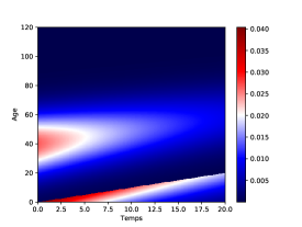
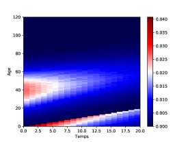
Figure 3. Left: true population density $g$. Right: ${\widehat{g}}^{N}_{{\widehat{h}}^{N}}$ with $N=4000$ over a single simulation of $Z^{N}$. $X$-axis, $Y$-axis: units in years.

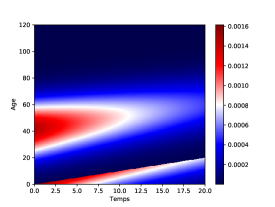
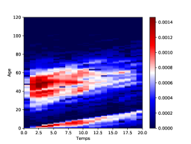
Figure 4. Left: true $\pi=\mu\cdot g$. Right: implementation of ${\widehat{\pi}}^{N}_{\widehat{\boldsymbol{h}}^{N}}$ with $N=4000$. $X$-axis, $Y$-axis: units in years.

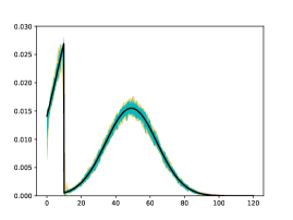
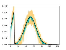
Figure 5. For fixed $t=10$, and $N=4000$, comparison between the true function (solid black) and a (pointwise) $95\%$ confidence interval based on 50 Monte-Carlo simulations. Oracle estimator in green and our adaptative estimator in yellow. Left: Estimation of $a\mapsto g(10,a)$. Right: Estimation of $a\mapsto\pi(10,a)=\mu(10,a)g(10,a)$. $X$-axis: units in years, Y-axis: rate per unit of time.

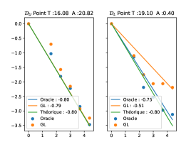
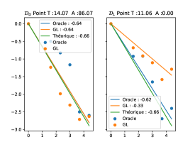
Figure 6. $\log_{10}$-integrated error of pointwise estimation against approximatively $\log_{10}N$ based on 50 Monte-carlo simulations. We compare the theoretical line given by the minimax theory (green) with a linear regression given by the oracle estimation (blue) and our estimation method (orange) for different values of $\log_{10}N$ at two given points in $\mathcal{D}_{L}$ and $\mathcal{D}_{U}$ respectively. Left: estimation of $g(t,a)$ at $(t,a)=(16.08,20.82)$ and $(t,a)=(19.10,0.40)$. Right: estimation for $\pi(t,a)=\mu(t,a)g(t,a)$ at $(t,a)=(14.07,86.07)$ and $(t,a)=(11.06,0.00)$. X-axis: integers $0$ to $5$ correspond to $N=10^{2},5\cdot 10^{2},10^{3},2\cdot 10^{3},4\cdot 10^{3},8\cdot 10^{3}$.

We end this section by exploring the estimation of $\mu$ via our quotient estimator.

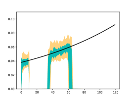
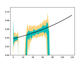
Figure 7. For fixed $t=10$, and $N=4000$, comparison between the true function (solid black) and a (pointwise) $95\%$ confidence interval based on 50 Monte-Carlo simulations. Oracle estimator in green and our adaptative estimator in yellow. Estimation of $a\mapsto\mu(10,a)$. Left: $\varpi=10^{-2}$. Right: $\varpi=5\cdot 10^{-3}$. $X$-axis: units in years, Y-axis: rate per unit of time. In order to improve on these results, one must either lower down $\varpi$ or expect to be in a more favourable regime $N\gg 4000$.

6. Proof or Theorem 6

This section is devoted to the proof of the concentration properties of the model stated in Theorem 6. Recall that $w_{1}\in\mathcal{L}_{\mathcal{D}}^{{\small\mathrm{\,time}}}$ and $w_{2}\in\mathcal{L}_{\mathcal{D}}^{{\small\mathrm{\,age}}}$ are two continuous weight functions. We introduce two fundamental processes for which we will establish concentration properties:

$$\mathcal{M}_{\,w_{1},w_{2}}^{N}(\mathcal{F})_{t}=\sup_{f\in\mathcal{F}}\big{|}\int_{0}^{t}w_{1}(s)M_{s}^{N}\big{(}w_{2}(s-\cdot)f_{s}\big{)}ds\big{|},$$

where $M_{t}^{N}(f)$ is defined in (39) below and

$$\mathcal{M}_{w_{2}}^{N}(\mathcal{F})_{t}=\sup_{f\in\mathcal{F}}\big{|}M_{t}^{N}\big{(}w_{2}(t-\cdot)f_{t}\big{)}\big{|}.$$

6.1. A first stability result

Proposition 21.

Work under Assumptions 1 and 2. Then $\mathcal{W}_{w_{1},w_{2}}^{N}(\mathcal{F})_{T}$ is bounded above by

$$|w_{1}|_{1}\mathcal{W}_{w_{2}}^{N}(\mathcal{F})_{0}+c_{0}^{-1}\int_{0}^{T}|w_{1}(t)|\big{(}\mathcal{W}_{w_{2},1}^{N}(\mathcal{F})_{t}+\mathcal{W}_{1,w_{2}}^{N}(\mathcal{F})_{t}\big{)}dt+\mathcal{M}_{\,w_{1},w_{2}}^{N}(\mathcal{F})_{T},$$

where $c_{0}$ is defined in Assumption 2.

Proof.

By (10), the action $\langle Z^{N}_{t},f_{t}\rangle$ of $Z_{t}^{N}(da)$ for $f\in\mathcal{L}_{\mathcal{D}}^{\infty}$ can be written as

$$\langle Z^{N}_{t},f_{t}\rangle =\int_{0}^{\infty}f_{t}(t+a)Z_{0}^{N}(da)$$

(38) $$+\int_{0}^{t}\int_{0}^{\infty}\big{(}b(s,a)f_{t}(t-s)-\mu(s,a)f_{t}(a+t-s)\big{)}Z^{N}_{s}(da)ds+M_{t}^{N}(f_{t}),$$

with

(39) $$M_{t}^{N}(f_{t})=N^{-1}\int_{0}^{t}\int_{\{i\leq n^{N}_{s^{-}}\}\times\mathbb{R}_{+}}\big{(}f_{t}(t-s){\bf 1}_{\{\theta\leq b\}}-f_{t}(a_{i}(Z^{N}_{s^{-}})+t-s){\bf 1}_{\{b\leq\theta\leq b+\mu\}}\big{)}\widetilde{\mathcal{Q}}(ds,di,d\theta).$$

In the above formula, $n_{t}^{N}=N\langle Z_{t}^{N},{\bf 1}\rangle$ is the size of the population at time $t$, the functions $b$ and $\mu$ in the indicators are evaluated at points $(s,a_{i}(Z^{N}_{s^{-}}))$ and $\widetilde{\mathcal{Q}}(ds,di,d\theta)={\mathcal{Q}}(ds,di,d\vartheta)-ds\big{(}\sum_{k\geq 1}\delta_{k}(di)\big{)}d\vartheta$ is the compensated measure of the Poisson measure ${\mathcal{Q}}$.

Apply now (38) to the test function $a\mapsto w_{2}(t-a)f_{t}(a)$ with $f\in\mathcal{F}$, substract $g(t,a)da$ in the equation above, noting that $g(t,a)$ solves (5), set $\eta^{N}_{t}(da)=Z^{N}_{t}(da)-g(t,a)da$ and obtain

$$\int_{\mathbb{R}_{+}}w_{2}(t-a)f_{t}(a)\eta^{N}_{t}(da)=\int_{\mathbb{R}_{+}}w_{2}(-a)f_{t}(t+a)\eta^{N}_{0}(da)$$

$$+\int_{0}^{t}\int_{\mathbb{R}_{+}}\big{(}w_{2}(s)f_{t}(t-s)b(s,a)-w_{2}(s-a)f_{t}(a+t-s)\mu(s,a)\big{)}\eta_{s}^{N}(da)ds+M_{t}^{N}(w_{2}(t-\cdot)f_{t}).$$

Multiplying each term by $\omega_{1}(t)$, integrating from $0$ to $T$ and taking absolute values, we also have

$$\big{|}\int_{0}^{T}w_{1}(t)\int_{\mathbb{R}_{+}}w_{2}(t-a)f_{t}(a)\eta^{N}_{t}(da)dt\big{|}\leq I+II+III+IV,$$

with

$$I =\big{|}\int_{0}^{T}w_{1}(t)\int_{\mathbb{R}_{+}}w_{2}(-a)f_{t}(t+a)\eta^{N}_{0}(da)dt\big{|},$$

$$II =\big{|}\int_{0}^{T}w_{1}(t)\int_{0}^{t}\int_{\mathbb{R}_{+}}w_{2}(s)f_{t}(t-s)b(s,a)\eta_{s}^{N}(da)dsdt\big{|},$$

$$III =\big{|}\int_{0}^{T}w_{1}(t)\int_{0}^{t}\int_{\mathbb{R}_{+}}w_{2}(s-a)f_{t}(a+t-s)\mu(s,a)\eta_{s}^{N}(da)dsdt\big{|},$$

$$IV =\big{|}\int_{0}^{T}w_{1}(t)M_{t}^{N}(w_{2}(t-\cdot)f_{t})dt\big{|}.$$

By Assumption 2, we have $f_{t}(t+a)\in\mathcal{F}$ therefore $I\leq\mathcal{W}_{w_{2}}^{N}(\mathcal{F})_{0}$. Using that $c_{0}f_{t}(t-s)b(s,a)\in\mathcal{F}$, we also have

$$\big{|}\int_{0}^{t}\int_{\mathbb{R}_{+}}w_{2}(s)f_{t}(t-s)b(s,a)\eta_{s}^{N}(da)ds\big{|} \leq c_{0}^{-1}\sup_{f\in\mathcal{F}}\big{|}\int_{0}^{t}\int_{\mathbb{R}_{+}}w_{2}(s){\bf 1}(s-a)f_{t}(a)\eta_{s}^{N}(da)ds\big{|}$$

$$=c_{0}^{-1}\mathcal{W}_{w_{2},1}(\mathcal{F})_{t},$$

Therefore $II\leq c_{0}^{-1}\int_{0}^{T}|w_{1}(t)|\mathcal{W}_{w_{2},1}(\mathcal{F})_{t}dt$. In the same way,

$$\big{|}\int_{0}^{t}\int_{\mathbb{R}_{+}}w_{2}(s-a)f_{t}(a+t-s)\mu(s,a)\eta_{s}^{N}(da)ds\big{|} \leq c_{0}^{-1}\sup_{f\in\mathcal{F}}\big{|}\int_{0}^{t}\int_{\mathbb{R}_{+}}{\bf 1}(s)w_{2}(s-a)f_{t}(a)\eta_{s}^{N}(da)ds\big{|}$$

$$=c_{0}^{-1}\mathcal{W}_{1,w_{2}}(\mathcal{F})_{t}$$

and $III\leq c_{0}^{-1}\int_{0}^{T}|w_{1}(t)|\mathcal{W}_{1,w_{2}}(\mathcal{F})_{t}dt$ follows likewise. Finally,

$$|IV|\leq\sup_{f\in\mathcal{F}}\big{|}\int_{0}^{T}w_{1}(t)M_{t}^{N}(w_{2}(t-\cdot)f_{t})dt\big{|}=\mathcal{M}_{\,w_{1},w_{2}}^{N}(\mathcal{F})_{t}.$$

Summing up the estimates, we obtain the conclusion noting that

$$\sup_{f\in\mathcal{F}}\big{|}\int_{0}^{T}w_{1}(t)\int_{\mathbb{R}_{+}}w_{2}(t-a)f_{t}(a)\eta_{s}^{N}(da)ds\big{|}=\mathcal{W}_{w_{1},w_{2}}^{N}(\mathcal{F})_{T}$$

since $\mathcal{F}$ is stable under $f\mapsto-f$ by Assumption 2. ∎

Proposition 22.

Work under Assumptions 1 and 2 . We have

$$\mathcal{W}_{w_{1},w_{2}}^{N}(\mathcal{F})_{T}\lesssim|w_{1}|_{1}\max_{(k_{1},k_{2})}|k_{1}|_{L^{1}([0,T])}\mathcal{W}_{k_{2}}^{N}(\mathcal{F})_{0}+\max_{(l_{1},\ldots,l_{4})}|l_{1}|_{L^{1}([0,T])}|l_{2}|_{L^{1}([0,T])}\mathcal{M}_{l_{3},l_{4}}^{N}(\mathcal{F})_{T},$$

where $(k_{1},k_{2})$ and $(l_{1},\ldots,l_{4})$ range over permutations of $(1,w_{2})$ and $(1,1,w_{1},w_{2})$ respectively. The symbol $\lesssim$ means inequality up to an explicitly computable constant depending on $T$ and $c_{0}$ from Assumption 2.

Proof.

Apply first Proposition 21 with $w_{1}=1$ and $w_{2}=1$ to obtain

$$\mathcal{W}_{1,1}^{N}(\mathcal{F})_{T} \leq T\mathcal{W}_{1}^{N}(\mathcal{F})_{0}+2c_{0}^{-1}\int_{0}^{T}\mathcal{W}_{1,1}^{N}(\mathcal{F})_{t}dt+\mathcal{M}_{1,1}^{N}(\mathcal{F})_{T}$$

$$\leq\big{(}T\mathcal{W}_{1}^{N}(\mathcal{F})_{0}+\mathcal{M}_{1,1}^{N}(\mathcal{F})_{T}\big{)}e^{2c_{0}^{-1}T}$$

$$=\mathcal{G}^{(1),N}(\mathcal{F})_{T},$$

say, by Grönwall lemma. Next, by Proposition 21 applied to $(w_{2},1)$, we obtain

$$\mathcal{W}_{w_{2},1}^{N}(\mathcal{F})_{T} \leq|w_{2}|_{L^{1}([0,T])}\mathcal{W}_{1}^{N}(\mathcal{F})_{0}+2c_{0}^{-1}\int_{0}^{T}|w_{2}(t)|\mathcal{W}_{1,1}^{N}(\mathcal{F})_{t}dt+\mathcal{M}_{w_{2},1}^{N}(\mathcal{F})_{T}$$

$$\leq|w_{2}|_{L^{1}([0,T])}\big{(}\mathcal{W}_{1}^{N}(\mathcal{F})_{0}+2c_{0}^{-1}\mathcal{G}^{(1),N}(\mathcal{F})_{T}\big{)}+\mathcal{M}_{w_{2},1}^{N}(\mathcal{F})_{T}$$

$$=\mathcal{G}^{(2),N}_{w_{2}}(\mathcal{F})_{T},$$

say. Apply now Proposition 21 with $(1,w_{2})$ so that

$$\mathcal{W}_{1,w_{2}}^{N}(\mathcal{F})_{T} \leq T\mathcal{W}_{w_{2}}^{N}(\mathcal{F})_{0}+c_{0}^{-1}\int_{0}^{T}\big{(}\mathcal{W}_{w_{2},1}^{N}(\mathcal{F})_{t}+\mathcal{W}_{1,w_{2}}^{N}(\mathcal{F})_{t}\big{)}dt+\mathcal{M}_{1,w_{2}}^{N}(\mathcal{F})_{T}$$

$$\leq T\mathcal{W}_{w_{2}}^{N}(\mathcal{F})_{0}+c_{0}^{-1}T\mathcal{G}^{(2),N}_{w_{2}}(\mathcal{F})_{T}+\int_{0}^{T}\mathcal{W}_{1,w_{2}}^{N}(\mathcal{F})_{t}dt+\mathcal{M}_{1,w_{2}}^{N}(\mathcal{F})_{T}$$

$$\leq\big{(}T\mathcal{W}_{w_{2}}^{N}(\mathcal{F})_{0}+CT\mathcal{G}^{(2),N}_{w_{2}}(\mathcal{F})_{T}+\mathcal{M}_{1,w_{2}}^{N}(\mathcal{F})_{T}\big{)}e^{c_{0}^{-1}T}$$

$$=\mathcal{G}^{(3),N}_{w_{2}}(\mathcal{F})_{T}$$

say, by the previous estimate and Grönwall lemma again. By Proposition 21 and the two previous bounds, we infer that $\mathcal{W}_{w_{1},w_{2}}^{N}(\mathcal{F})_{T}$ is less than

$$|w_{1}|_{L^{1}([0,T])}\mathcal{W}_{w_{2}}^{N}(\mathcal{F})_{0}+c_{0}^{-1}|w_{1}|_{L^{1}([0,T])}\big{(}\mathcal{G}^{(2),N}_{w_{2}}(\mathcal{F})_{T}+\mathcal{G}^{(3),N}_{w_{2}}(\mathcal{F})_{T}\big{)}+\mathcal{M}_{\,w_{1},w_{2}}^{N}(\mathcal{F})_{T}.$$

Expanding the estimates $\mathcal{G}^{(2),N}_{w_{2}}(\mathcal{F})_{T}$ and $\mathcal{G}^{(3),N}_{w_{2}}(\mathcal{F})_{T}$ in terms of their appropriate arguments concludes the proof. ∎

By Proposition 22, we see that the stability of the system is controlled by the initial approximation $\mathcal{W}_{w_{2}}^{N}(\mathcal{F})_{0}$ (including $w_{2}=1$) and the propagation of the stochastic term $\mathcal{M}_{w_{1},w_{2}}^{N}(\mathcal{F})_{T}$. We now turn to that latter term.

6.2. Stability of the stochastic term

For $f\in\mathcal{L}^{\small{\mathrm{\,age}}}_{\mathcal{D}}$, let

$$\widetilde{\mathcal{M}}_{\,w_{1},w_{2}}^{N}(f)_{t}=\int_{0}^{t}w_{1}(s)M_{s}^{N}\big{(}w_{2}(s-\cdot)f\big{)}ds$$

and

$$\widetilde{\mathcal{M}}_{\,w_{2}}^{N}(f)_{t}=M_{t}^{N}\big{(}w_{2}(t-\cdot)f\big{)}.$$

In particular, since $\mathcal{F}$ is stable under $f\mapsto-f$, we have

(40) $$\sup_{f\in\mathcal{F}}\widetilde{\mathcal{M}}_{\,w_{1},w_{2}}^{N}(f)_{T}=\sup_{f\in\mathcal{F}}\big{|}\widetilde{\mathcal{M}}_{\,w_{1},w_{2}}^{N}(f)_{T}\big{|}=\mathcal{M}_{\,w_{2}}^{N}(\mathcal{F})_{T}$$

and

$$\sup_{f\in\mathcal{F}}\widetilde{\mathcal{M}}_{\,w_{2}}^{N}(f)_{T}=\sup_{f\in\mathcal{F}}\big{|}\widetilde{\mathcal{M}}_{\,w_{2}}^{N}(f)_{T}\big{|}=\mathcal{M}_{\,w_{2}}^{N}(\mathcal{F})_{T}.$$

For $\kappa\geq 0$, consider the event

(41) $$\mathcal{A}^{N}_{\kappa}=\big{\{}\sup_{0\leq t\leq T}\langle Z_{t}^{N},{\bf 1}\rangle\leq\exp(|b|_{\infty}T)(1+\kappa)\big{\}},$$

and for $\lambda\geq 0$, set

$$\vartheta_{w_{1},w_{2}}^{N}(f)_{\lambda}=2NT|w_{1}|_{\infty}^{-1}\exp(|b|_{\infty}T)(|b|_{\infty}+|\mu|_{\infty}\big{)}\rho\big{(}N^{-1}\lambda|w_{1}w_{2}|_{\infty}|f|_{\infty}\big{)},$$

where $\rho(x)=e^{x}-x-1$.

Proposition 23.

Work under Assumptions 1. For large enough $N$, we have

(42) $$\int_{0}^{\infty}\mathbb{P}\big{(}(\mathcal{A}^{N}_{\kappa})^{c}\big{)}e^{\kappa}d\kappa\leq\tfrac{1}{2}$$

and for $\lambda\geq 0$,

(43) $$\mathbb{E}\big{[}\exp\big{(}\lambda\big{|}\widetilde{\mathcal{M}}_{\,w_{1},w_{2}}^{N}(f)_{T}-\widetilde{\mathcal{M}}_{\,w_{1},w_{2}}^{N}(g)_{T}\big{|}\big{)}{\bf 1}_{\mathcal{A}^{N}_{\kappa}}\big{]}\leq 2\exp\big{(}|w_{1}|_{1}(1+\kappa)\vartheta_{w_{1},w_{2}}^{N}(f-g)_{\lambda}\big{)}.$$

Moreover, (43) remains true with $\widetilde{\mathcal{M}}_{\,w_{2}}^{N}(f)_{T}-\widetilde{\mathcal{M}}_{\,w_{2}}^{N}(g)_{T}$, replacing formally $w_{1}$ by $1$ in the right-hand side of the inequality.

Proof.

We first prove (42), namely

$$\int_{0}^{\infty}e^{\kappa}\mathbb{P}\big{(}\sup_{0\leq t\leq T}\langle Z^{N}_{t},{\bf 1}\rangle>\exp(|b|_{\infty}T)(1+\kappa)\big{)}d\kappa\leq\tfrac{1}{2}.$$

Step 1) Consider the equation

$$\widetilde{Z}_{t}^{N}=\tau_{t}Z_{0}^{N}+N^{-1}\int_{0}^{t}\int_{\mathbb{N}\times\mathbb{R}_{+}}\delta_{t-s}(da){\bf 1}_{\{0\leq\vartheta\leq|b|_{\infty},i\leq N\langle\widetilde{Z}_{s^{-}}^{N},{\bf 1}\rangle\}}\mathcal{Q}_{1}(ds,di,d\vartheta)$$

defined on the same probability space as $(Z_{t}(da))_{0\leq t\leq T}$. Applying (38) with $b=|b|_{\infty}$, $\mu=0$ and $f_{t}=1$, we obtain

$$\langle\widetilde{Z}^{N}_{t},{\bf 1}\rangle=\langle\widetilde{Z}^{N}_{0},{\bf 1}\rangle+|b|_{\infty}\int_{0}^{t}\langle\widetilde{Z}^{N}_{s},{\bf 1}\rangle ds+M_{t}^{N}(\bf{1}),$$

and for every $\lambda\geq 0$, by Itô’s formula:

$$\exp\big{(}\lambda\langle\widetilde{Z}^{N}_{t},{\bf 1}\rangle\big{)}=\exp\big{(}\lambda\langle\widetilde{Z}^{N}_{0},{\bf 1}\rangle\big{)}+N|b|_{\infty}\big{(}e^{\lambda/N}-1\big{)}\int_{0}^{t}\langle\widetilde{Z}^{N}_{s},{\bf 1}\rangle\exp\big{(}\lambda\langle\widetilde{Z}^{N}_{s},{\bf 1}\rangle\big{)}ds+\xi_{t},$$

where $(\xi_{t})_{0\leq t\leq T}$ is a local martingale. By localisation, one can prove that $\mathbb{E}[\xi_{t}]=0$. Writing $f(t,\lambda)=\mathbb{E}[\exp\big{(}\lambda\langle\widetilde{Z}^{N}_{t},{\bf 1}\rangle\big{)}]$, it follows that

(44) $$f(t,\lambda)=f(0,\lambda)+N|b|_{\infty}\big{(}e^{\lambda/N}-1\big{)}\int_{0}^{t}\partial_{\lambda}f(s,\lambda)ds.$$

The solution of the transport equation (44) at time $t=T$ with initial condition $f(0,\lambda)=f_{0}(\lambda)$ is given by

$$f(T,\lambda) =f_{0}\Big{(}N\log\frac{e^{\lambda/N-|b|_{\infty}T}}{1-(1-e^{-|b|_{\infty}T})e^{\lambda/N}}\Big{)}\leq\exp\Big{(}qN\log\frac{e^{\lambda/N-|b|_{\infty}T}}{1-(1-e^{-|b|_{\infty}T})e^{\lambda/N}}\Big{)},$$

where the last inequality stems from $f_{0}(\lambda)=\mathbb{E}[\exp(\lambda\langle\widetilde{Z}_{0}^{N},{\bf 1}\rangle)]=\mathbb{E}[\exp(\lambda\langle Z_{0}^{N},{\bf 1}\rangle)]\leq e^{q\lambda}$ for some $q$ by Assumption 1 (ii).

Step 2) With the notation $r=\exp(-|b|_{\infty}T)$, the usual Chernoff bound argument yields

$$\log\mathbb{P}\big{(}\langle\widetilde{Z}^{N}_{T},{\bf 1}\rangle>r^{-1}(1+\kappa)\big{)}\leq \,-\lambda r^{-1}(1+\kappa)+qN\log\tfrac{re^{\lambda/N}}{1-(1-r)e^{\lambda/N}}$$

$$\leq \,-Nr^{-1}(1+\kappa)\log\big{(}\big{(}1-\tfrac{rq}{\kappa+1}\big{)}\tfrac{1}{1-r}\big{)}+qN\log\tfrac{\kappa+1-rq}{1-r}$$

$$\leq \,\log C_{1}-C_{2}N\kappa$$

for the choice $\lambda=N\log\big{(}(1-\frac{rq}{\kappa+1})\frac{1}{1-r}\big{)}$ and for two constants $C_{i}=C_{i}(q,r)>0$ that do not depend on $N$. Noting that by construction, $\sup_{t\leq T}\langle Z^{N}_{t},{\bf 1}\rangle\leq\langle\widetilde{Z}^{N}_{T},{\bf 1}\rangle$, we finally obtain

$$\int_{0}^{\infty}e^{\kappa}\mathbb{P}\big{(}\sup_{0\leq t\leq T}\langle Z^{N}_{t},{\bf 1}\rangle>r^{-1}(1+\kappa)\big{)}d\kappa \leq\int_{0}^{\infty}e^{\kappa}\mathbb{P}\big{(}\langle\widetilde{Z}^{N}_{T},{\bf 1}\rangle>r^{-1}(1+\kappa)\big{)}d\kappa$$

$$\leq C_{1}\int_{0}^{\infty}e^{(1-C_{2}N)\kappa}d\kappa=\frac{C_{1}}{C_{2}N-1}\leq\tfrac{1}{2}$$

for $N\geq(1+2C_{1})/C_{2}$, and (42) is proved.

Step 3) We now turn to (43). For $t_{0}\in[0,T]$ and $f\in\mathcal{L}_{\mathcal{D}}^{\small{\mathrm{\,age}}}$, define

(45) $$B_{t,t_{0}}^{N}(f)=N\int_{0}^{t\wedge t_{0}}\int_{\mathbb{R}_{+}}\Big{(}b(s,a)\rho\big{(}N^{-1}f(t_{0}-s)\big{)}+\mu(s,a)\rho\big{(}N^{-1}f(a+t_{0}-s)\big{)}\Big{)}Z_{s}^{N}(da)ds.$$

Lemma 24.

For every $t_{0}\in[0,T]$ and $f,g\in\mathcal{L}_{\mathcal{D}}^{\small{\mathrm{\,age}}}$, there exists a nonnegative random variable $\Lambda_{t_{0},t_{0}}^{N}(f-g)$ with $\mathbb{E}[\Lambda_{t_{0},t_{0}}^{N}(f-g)]=1$ such that

$$\mathbb{E}\big{[}\exp\big{(}M_{t_{0}}^{N}(f)-M_{t_{0}}^{N}(g)\big{)}\big{]}=\mathbb{E}\big{[}\Lambda_{t_{0},t_{0}}^{N}(f-g)\exp B_{t_{0},t_{0}}^{N}(f-g)\big{]}.$$

Proof.

Fix $t_{0}\in[0,T]$ and for $f\in\mathcal{L}_{\mathcal{D}}^{\small{\mathrm{\,age}}}$, define the random process

$$\widetilde{M}_{t,t_{0}}^{N}(f)=N^{-1}\int_{0}^{t\wedge t_{0}}\int_{\{i\leq n^{N}_{s^{-}}\}\times\mathbb{R}_{+}}\big{(}f(t_{0}-s){\bf 1}_{\{b\leq\theta\}}-f(a_{i}(Z^{N}_{s^{-}})+t_{0}-s){\bf 1}_{\{b\leq\theta\leq b+\mu\}}\big{)}\widetilde{\mathcal{Q}}(ds,di,d\theta),$$

obtained by keeping $t=t_{0}$ fixed in the integrand of $M_{t\wedge t_{0}}^{N}(f)$ defined in (39). By construction, $(\widetilde{M}_{t,t_{0}}(f))_{0\leq t\leq T}$ is a martingale. In turn, a simple consequence of Itô’s formula, see e.g. Tran [43] shows that the random process

$$t\mapsto\Lambda_{t,t_{0}}^{N}(f)=\exp\big{(}\widetilde{M}_{t,t_{0}}^{N}(f)-B_{t,t_{0}}^{N}(f)\big{)}$$

is a martingale such that $\mathbb{E}[\Lambda_{t,t_{0}}^{N}(f)]=1$. Noting that $M_{t_{0}}^{N}(f)=\widetilde{M}_{t_{0},t_{0}}^{N}(f)$ at $t=t_{0}$, we also have

$$\mathbb{E}\big{[}\exp\big{(}M_{t_{0}}^{N}(f)-M_{t_{0}}^{N}(g)\big{)}\big{]} =\mathbb{E}\big{[}\exp\big{(}M_{t_{0}}^{N}(f-g)\big{)}\big{]}$$

$$=\mathbb{E}\big{[}\exp\big{(}\widetilde{M}_{t_{0},t_{0}}^{N}(f-g)\big{)}\big{]}$$

$$=\mathbb{E}\big{[}\Lambda_{t_{0},t_{0}}^{N}(f-g)\exp B_{t_{0},t_{0}}^{N}(f-g)\big{]}.$$

∎

Let $\lambda\geq 0$. We substitute $f-g$ by $a\mapsto\lambda w_{1}(t_{0})w_{2}(t_{0}-a)(f(a)-g(a))$ and look for an upper bound for

$$B_{t_{0},t_{0}}^{N}\big{(}\lambda w_{1}(t_{0})w_{2}(t_{0}-\cdot)(f-g)\big{)}.$$

Step 4) Observe first that $\rho(x)=e^{x}-x-1$ implies that for any nonnegative function $\psi\in\mathcal{L}_{\mathcal{D}}^{\small{\mathrm{\,age}}}$, we have

$$\rho\big{(}N^{-1}\lambda\psi(a^{\prime})(f(a)-g(a))\big{)} \leq N^{-1}\psi(a^{\prime})|f-g|_{\infty}\int_{0}^{\lambda}\big{(}\exp(\kappa N^{-1}|\psi|_{\infty}|f-g|_{\infty})-1\big{)}d\kappa$$

$$=\frac{\psi(a^{\prime})}{|\psi|_{\infty}}\rho\big{(}N^{-1}\lambda|\psi|_{\infty}|f-g|_{\infty}\big{)}.$$

Therefore, with $\psi(a^{\prime})=w_{1}(t_{0})w_{2}(t_{0}-a^{\prime})$ and $a^{\prime}=t_{0}-s$, we derive

$$\rho\big{(}N^{-1}\lambda w_{1}(t_{0})w_{2}(s)(f(t_{0}-s)-g(t_{0}-s))\big{)}\leq\frac{w_{1}(t_{0})w_{2}(s)}{|w_{1}w_{2}|_{\infty}}\rho\big{(}N^{-1}\lambda|w_{1}w_{2}|_{\infty}|f-g|_{\infty}\big{)}$$

and

$$\rho\big{(}N^{-1}\lambda w_{1}(t_{0})w_{2}(s-a)(f(a+t_{0}-s)-g(a+t_{0}-s))\big{)}\leq\frac{w_{1}(t_{0})w_{2}(s-a)}{|w_{1}w_{2}|_{\infty}}\rho\big{(}N^{-1}\lambda|w_{1}w_{2}|_{\infty}|f-g|_{\infty}\big{)}$$

with $a^{\prime}=a+t_{0}-s$ follows likewise. Plugging these two estimates in the definition (45) of $B_{t_{0},t_{0}}^{N}$, we infer on $\mathcal{A}^{N}_{\kappa}=\{\sup_{0\leq t\leq T}\langle Z^{N}_{t},{\bf 1}\rangle\leq\exp(|b|_{\infty}T)(1+\kappa)\}$ the chain of inequalities

$$B_{t_{0},t_{0}}^{N}\big{(}\lambda w_{1}(t_{0})w_{2}(t_{0}-\cdot)(f-g)\big{)}$$

$$\leq \,N(|b|_{\infty}+|\mu|_{\infty})\frac{w_{1}(t_{0})}{|w_{1}w_{2}|_{\infty}}\rho\big{(}N^{-1}\lambda|w_{1}w_{2}|_{\infty}|f-g|_{\infty}\big{)}\int_{0}^{t_{0}}\int_{\mathbb{R}_{+}}\big{(}w_{2}(s)+w_{2}(s-a)\big{)}Z_{s}^{N}(da)ds$$

$$\leq \,N(|b|_{\infty}+|\mu|_{\infty})\frac{w_{1}(t_{0})}{|w_{1}|_{\infty}}\rho\big{(}N^{-1}\lambda|w_{1}w_{2}|_{\infty}|f-g|_{\infty}\big{)}2T\sup_{0\leq t\leq T}\langle Z_{t}^{N},{\bf 1}\rangle$$

$$\leq \,N(|b|_{\infty}+|\mu|_{\infty})\frac{w_{1}(t_{0})}{|w_{1}|_{\infty}}\rho\big{(}N^{-1}\lambda|w_{1}w_{2}|_{\infty}|f-g|_{\infty}\big{)}\exp(|b|_{\infty}T)(1+\kappa)2T$$

$$= \,w_{1}(t_{0})(1+\kappa)\vartheta_{w_{1},w_{2}}^{N}(f-g)_{\lambda}.$$

We derive

(46) $$\exp\big{(}\lambda w_{1}(t_{0})M_{t_{0}}^{N}(w_{2}(t_{0}-\cdot)(f-g))\big{)}{\bf 1}_{\mathcal{A}^{N}_{\kappa}}$$

$$\leq \exp\big{(}w_{1}(t_{0})(1+\kappa)\vartheta_{w_{1},w_{2}}^{N}(f-g)_{\lambda}\big{)}\Lambda_{t_{0},t_{0}}^{N}(\lambda w_{1}(t_{0})w_{2}(t_{0}-\cdot)(f-g)\big{)}{\bf 1}_{\mathcal{A}^{N}_{\kappa}}.$$

Step 5) For every integer $n\geq 1$ and $\lambda\geq 0$, $f\in\mathcal{L}_{\mathcal{D}}^{\small{\mathrm{\,age}}}$, define

$$\Delta^{N,n}_{w_{1},w_{2}}(f-g)_{\lambda}=\exp\big{(}\lambda Tn^{-1}\sum_{i=1}^{n}w_{1}(iTn^{-1})M_{iTn^{-1}}^{N}(w_{2}(iTn^{-1}-\cdot)(f-g))\big{)}.$$

Applying repeatedly (46) with $t_{0}=iTn^{-1}$ and integrating with respect to $\mathbb{E}_{\mathcal{A}^{N}_{\kappa}}[\cdot]=\mathbb{P}(\mathcal{A}^{N}_{\kappa})^{-1}\mathbb{E}[\cdot{\bf 1}_{\mathcal{A}^{N}_{\kappa}}]$, we obtain

$$\mathbb{E}_{\mathcal{A}^{N}_{\kappa}}\big{[}\Delta^{N,n}_{w_{1},w_{2}}(f-g)_{\lambda}\big{]}\leq \;\exp\big{(}Tn^{-1}\sum_{i=1}^{n}w_{1}(iTn^{-1})(1+\kappa)\vartheta_{w_{1},w_{2}}^{N}(f-g)_{\lambda}\big{)}\times$$

$$\times\mathbb{E}_{\mathcal{A}^{N}_{\kappa}}\Big{[}\prod_{i=1}^{n}\Lambda_{iTn^{-1},iTn^{-1}}^{N}(\lambda Tw_{1}(t_{0})w_{2}(t_{0}-\cdot)(f-g)\big{)}^{1/n}\Big{]}$$

$$\leq \;\exp\big{(}Tn^{-1}\sum_{i=1}^{n}w_{1}(iTn^{-1})(1+\kappa)\vartheta_{w_{1},w_{2}}^{N}(f-g)_{\lambda}\big{)}\mathbb{P}\big{(}\mathcal{A}^{N}_{\kappa}\big{)}^{-1},$$

where we used the fact that the geometric mean is controlled by the arithmetic mean:

$$\prod_{i=1}^{n}\Lambda_{iTn^{-1},iTn^{-1}}^{N}(\lambda w_{1}(t_{0})w_{2}(t_{0}-\cdot)(f-g)\big{)}^{1/n}\leq n^{-1}\sum_{i=1}^{n}\Lambda_{iTn^{-1},iTn^{-1}}^{N}(\lambda w_{1}(t_{0})w_{2}(t_{0}-\cdot)(f-g)\big{)}$$

and the fact that

$$\mathbb{E}_{\mathcal{A}^{N}_{\kappa}}\Big{[}\Lambda_{iTn^{-1},iTn^{-1}}^{N}(\lambda w_{1}(t_{0})w_{2}(t_{0}-\cdot)(f-g)\big{)}\Big{]}$$

$$\leq \;\mathbb{P}\big{(}\mathcal{A}^{N}_{\kappa}\big{)}^{-1}\mathbb{E}\Big{[}\Lambda_{iTn^{-1},iTn^{-1}}^{N}(\lambda w_{1}(t_{0})w_{2}(t_{0}-\cdot)(f-g)\big{)}\Big{]}=\mathbb{P}\big{(}\mathcal{A}^{N}_{\kappa}\big{)}^{-1}$$

since $\Lambda_{iTn^{-1},iTn^{-1}}^{N}(\lambda w_{1}(t_{0})w_{2}(t_{0}-\cdot)(f-g)\big{)}$ has expectation $1$ by Lemma 24. Using

$$\liminf_{n\rightarrow\infty}\Delta^{N,n}_{w_{1},w_{2}}(f-g)_{\lambda}=\exp\big{(}\lambda\int_{0}^{T}w_{1}(s)M_{s}^{N}(w_{2}(s-\cdot)(f-g))ds\big{)}$$

by convergence of Riemann sums, letting $n\rightarrow\infty$, we obtain by Fatou lemma

(47) $$\mathbb{E}_{\mathcal{A}^{N}_{\kappa}}\Big{[}\exp\big{(}\lambda\int_{0}^{T}w_{1}(s)M_{s}^{N}(w_{2}(s-\cdot)(f-g))ds\big{)}\Big{]}\leq\mathbb{P}\big{(}\mathcal{A}^{N}_{\kappa}\big{)}^{-1}\exp\big{(}|w_{1}|_{1}(1+\kappa)\vartheta_{w_{1},w_{2}}^{N}(f-g)_{\lambda}\big{)}.$$

Noting that Lemma 24 also holds for $-M_{s}^{N}(f)$ and applying (47) to $-M_{s}^{N}(w_{2}(s-\cdot)(f-g))$, we infer

$$\mathbb{E}_{\mathcal{A}^{N}_{\kappa}}\Big{[}\exp\big{(}\lambda\big{|}\int_{0}^{T}w_{1}(s)M_{s}^{N}\big{(}w_{2}(s-\cdot)(f-g)\big{)}ds\big{|}\big{)}\Big{]}\leq 2\mathbb{P}\big{(}\mathcal{A}^{N}_{\kappa}\big{)}^{-1}\exp\big{(}|w_{1}|_{1}(1+\kappa)\vartheta_{w_{1},w_{2}}^{N}(f-g)_{\lambda}\big{)},$$

but since $\int_{0}^{T}w_{1}(s)M_{s}^{N}\big{(}w_{2}(s-\cdot)(f-g)\big{)}ds=\widetilde{\mathcal{M}}_{w_{1},w_{2}}^{N}(f)_{T}-\widetilde{\mathcal{M}}_{w_{1},w_{2}}^{N}(g)_{T}$, the estimate (43) is established.

Step 6) It remains to prove (43) for $\mathcal{M}_{w_{2}}^{N}(f-g)_{T}$. We first integrate (46) for $w_{1}=1$ at $t_{0}=T$ so that $|w_{1}|_{1}=T$ and proceed exactly as in Step 5) to obtain

$$\mathbb{E}_{\mathcal{A}^{N}_{\kappa}}\big{[}\exp\big{(}\lambda M_{T}^{N}(w_{2}(T-\cdot)(f-g))\big{)}\big{]}\leq\mathbb{P}(\mathcal{A}^{N}_{\kappa})^{-1}\exp\big{(}T(1+\kappa)\vartheta_{1,w_{2}}^{N}(f-g)_{\lambda}\big{)}.$$

Applying the same argument for $-M_{T}^{N}$, we also have

$$\mathbb{E}_{\mathcal{A}^{N}_{\kappa}}\big{[}\exp\big{(}\lambda\big{|}M_{T}^{N}(w_{2}(T-\cdot)(f-g))\big{|}\big{)}\big{]}\leq 2\mathbb{P}(\mathcal{A}^{N}_{\kappa})^{-1}\exp\big{(}T(1+\kappa)\vartheta_{1,w_{2}}^{N}(f-g)_{\lambda}\big{)}$$

which is the desired result.

∎

Proposition 23 is the main ingredient to obtain a concentration inequality for the processes $(\widetilde{\mathcal{M}}_{\,w_{2}}^{N}(f)_{T})_{f\in\mathcal{F}}$ and $(\widetilde{\mathcal{M}}_{\,w_{1},w_{2}}^{N}(f)_{T})_{f\in\mathcal{F}}$, and in turn, a deviation bound for $\mathcal{M}_{w_{1},w_{2}}(\mathcal{F})_{T}$ and $\mathcal{M}_{w_{2}}(\mathcal{F})_{T}$ thanks to (40). The proof is given in Section 6.4 below.

More precisely, consider the apparently more general situation where we have a real-valued process $\xi(f)_{f\in\mathcal{F}}$ indexed by some metric set $(\mathcal{F},d)$ and a family of events $\mathcal{A}(\kappa)_{\kappa>0}$ satisfying the following properties:

(48) $$\int_{0}^{\infty}\mathbb{P}\big{(}\mathcal{A}(\kappa)^{c}\big{)}e^{\kappa}d\kappa\leq\tfrac{1}{2},$$

and

(49) $$\mathbb{E}\big{[}\exp\big{(}\lambda|\xi(f)-\xi(g)|\big{)}{\bf 1}_{\mathcal{A}(\kappa)}\big{]}\leq 2\exp\big{(}c_{1}(1+\kappa)\rho(c_{2}d(f,g)\lambda)\big{)},$$

for every $\lambda\geq 0$ and some $c_{1},c_{2}>0$.

Proposition 25.

Assume that $\xi(f)_{f\in\mathcal{F}}$ and $\mathcal{A}(\kappa)_{\kappa>0}$ satisfy (48) and (49) and that $\xi(f_{0})=0$ for some $f_{0}\in\mathcal{F}$. Then there exists a choice $\varpi=\varpi(c_{1},c_{2})>0$ such that for every $u\geq 0$:

$$\mathbb{P}\Big{(}\sup_{f\in\mathcal{F}}|\xi(f)|\geq 8\big{(}u+\int_{0}^{\mathrm{diam}_{\widetilde{d}}(\mathcal{F})}\log\big{(}1+\mathcal{N}(\mathcal{F},\widetilde{d},\epsilon)\big{)}d\epsilon\big{)}\Big{)}\leq\big{(}e^{u/\mathrm{diam}_{\widetilde{d}}(\mathcal{F})}-1\big{)}^{-1},$$

where $\widetilde{d}=\varpi\,d$, $\mathrm{diam}_{\widetilde{d}}(\mathcal{F})=\sup_{f,g\in\mathcal{F}}\widetilde{d}(f,g)$ and $\mathcal{N}(\mathcal{F},\widetilde{d},\epsilon)$ is the minimal number of balls of $\widetilde{d}$-size $\epsilon>0$ that are necessary to cover $\mathcal{F}$.

Remark 26.

We show in Remark 36 at the end of the proof of Proposition 25 that if $c_{1}\geq 308$, we may pick $\varpi(c_{1},c_{2})=k\sqrt{c_{1}}c_{2}$, with $k=2\sqrt{77}$.

The proof of Proposition 25 relies on standard concentration techniques and goes back to Dudley [14]. We use the classical textbook of Ledoux-Talagrand [28] and detail the computations in the Appendix section 8. Combining Proposition 23 and 25, we obtain the following

Theorem 27.

Work under Assumptions 1. Assume $\mathrm{diam}_{|\cdot|_{\infty}}\mathcal{F}\leq 1$ and

$$\mathrm{e}(\mathcal{F})=\int_{0}^{1}\log\big{(}1+\mathcal{N}(\mathcal{F},|\cdot|_{\infty},\epsilon)\big{)}d\epsilon<\infty.$$

For large enough $N$, there exists an explicit choice of $C=C(\mathrm{e}(\mathcal{F}),T,|b|_{\infty},|\mu|_{\infty})>0$, given in the proof below, such that for every $u\geq 0$:

(50) $$\mathbb{P}\big{(}\mathcal{M}_{\,w_{1},w_{2}}^{N}(\mathcal{F})_{T}\geq(1+u)CN^{-1/2}|w_{1}|_{1,\infty}|w_{2}|_{\infty}\big{)}\leq(e^{u\mathrm{e}(\mathcal{F})}-1)^{-1}$$

and

(51) $$\mathbb{P}\big{(}\mathcal{M}_{\,w_{2}}^{N}(\mathcal{F})_{T}\geq(1+u)CN^{-1/2}|w_{2}|_{\infty}\big{)}\leq(e^{u\mathrm{e}(\mathcal{F})}-1)^{-1}.$$

Proof.

We plan to apply Proposition 25 with $\xi(f)=\widetilde{\mathcal{M}}_{\,w_{1},w_{2}}^{N}(f)_{T}$, having $\xi(f_{0})=0$ for $f_{0}=0$. We take $\mathcal{A}(\kappa)=\mathcal{A}_{\kappa}^{N}$ defined in (41) and notice that (48) is satisfied by (42). Also, we have (49) by (43) with

(52) $$c_{1}=2NT|w_{1}|_{1}|w_{1}|_{\infty}^{-1}\exp(|b|_{\infty}T)(|b|_{\infty}+|\mu|_{\infty}\big{)}\;\;\text{and}\;\;c_{2}=|w_{1}w_{2}|_{\infty}N^{-1},$$

for the metric $d(f,g)=|f-g|_{\infty}$. Setting $\widetilde{d}=\varpi\,d$ with $\varpi$ taken from Proposition 25, we have $\mathrm{diam}_{\widetilde{d}}(\mathcal{F})=\varpi\,\mathrm{diam}_{d}(\mathcal{F})\leq\varpi$ by assumption and also $\mathcal{N}(\mathcal{F},\widetilde{d},\varepsilon)\leq\mathcal{N}(\mathcal{F},d,\varepsilon/\varpi)$. It follows that

$$\int_{0}^{\mathrm{diam}_{\widetilde{d}}(\mathcal{F})}\log\big{(}1+\mathcal{N}(\mathcal{F},\widetilde{d},\epsilon)\big{)}d\epsilon \leq\int_{0}^{\varpi}\log\big{(}1+\mathcal{N}(\mathcal{F},d,\epsilon/\varpi)\big{)}d\epsilon=\varpi\,\mathrm{e}(\mathcal{F}),$$

which is finite by assumption. Since $\mathcal{M}_{\,w_{1},w_{2}}^{N}(\mathcal{F})_{T}=\sup_{f\in\mathcal{F}}|\xi(f)|=\sup_{f\in\mathcal{F}}\xi(f)$, remember (40), we may apply Proposition 25 and obtain, for every $u\geq 0$,

$$\mathbb{P}\big{(}\mathcal{M}_{\,w_{1},w_{2}}^{N}(\mathcal{F})_{T}\geq 8(\varpi\,\mathrm{e}(\mathcal{F})+u)\big{)}\leq(e^{u/\varpi}-1)^{-1},$$

or equivalently

$$\mathbb{P}\big{(}\mathcal{M}_{\,w_{1},w_{2}}^{N}(\mathcal{F})_{T}\geq 8\varpi\,\mathrm{e}(\mathcal{F})(1+u)\big{)}\leq(e^{u\mathrm{e}(\mathcal{F})}-1)^{-1}.$$

By Remark 26 (see also Remark 36), we pick $\varpi=\varpi(c_{1},c_{2})=k\sqrt{c_{1}}c_{2}$ with $k=2\sqrt{77}$, assuming $c_{1}\geq 308$ which is satisfied for sufficiently large $N$ by (52). Using (52) again, it follows that

$$8k\sqrt{c_{1}}c_{2}\mathrm{e}(\mathcal{F})(1+u) =(1+u)8k\,\mathrm{e}(\mathcal{F})e^{\tfrac{1}{2}|b|_{\infty}T}\sqrt{2T}(|b|_{\infty}+|\mu|_{\infty})^{1/2}N^{-1/2}(|w_{1}|_{1}|w_{1}|_{\infty})^{1/2}|w_{2}|_{\infty}$$

$$=(1+u)CN^{-1/2}|w_{1}|_{1,\infty}|w_{2}|_{\infty},$$

say, with

(53) $$C=C(\mathrm{e}(\mathcal{F}),T,|b|_{\infty},|\mu|_{\infty})=8k\,\mathrm{e}(\mathcal{F})e^{\tfrac{1}{2}|b|_{\infty}T}\sqrt{2T}(|b|_{\infty}+|\mu|_{\infty})^{1/2}$$

and (50) follows. The proof of (51) is obtained in the same way and is omitted. ∎

Remark 28.

(i) Up to inflating the constant $C$ by a multiplicative factor $\max(1,\mathrm{e}(\mathcal{F}))$, we see that Theorem 27 implies a mild concentration property for

$$(|w_{1}|_{1,\infty}|w_{2}|_{\infty})^{-1}\mathcal{M}_{\,w_{1},w_{2}}^{N}(\mathcal{F})_{T}\;\;\text{and}\;\;|w_{2}|_{\infty}^{-1}\mathcal{M}_{\,w_{2}}^{N}(\mathcal{F})_{T}$$

with rate $CN^{-1/2}$.

(ii) The initial bound $|w_{2}|_{1,\infty}$ of Assumption 5 inflates to $|w_{2}|_{\infty}$ in (51). This defect actually has dramatic consequences when applied to subsequent statistical estimation: $w_{2}$ becomes a kernel depending on $N$ that mimicks a Dirac mass which is not stable for the $|\cdot|_{\infty}$ metric. Improving on this estimates is actually the key difficulty in the proof of Theorem 6.

6.3. Proof of Theorem 6

The weakness of Theorem 27 lies in the use of Proposition 23, where the control (43) somehow needs to be improved. This improvement however uses the results of Theorem 27 that we are going to iterate.

Step 1) By Proposition 22, we have $\mathcal{W}_{w_{1},w_{2}}^{N}(\mathcal{F})_{T}\lesssim I+II$, with

$$I=|w_{1}|_{1}\max_{(k_{1},k_{2})}|k_{1}|_{L^{1}([0,T])}\mathcal{W}_{k_{2}}^{N}(\mathcal{F})_{0}$$

and

$$II=\max_{(l_{1},\ldots,l_{4})}|l_{1}|_{L^{1}([0,T])}|l_{2}|_{L^{1}([0,T])}\mathcal{M}_{l_{3},l_{4}}^{N}(\mathcal{F})_{T}.$$

Since $|w_{1}|_{1}\max_{(k_{1},k_{2})}|k_{1}|_{L^{1}([0,T])}\mathcal{W}_{k_{2}}^{N}(\mathcal{F})_{0}\lesssim\max_{k=1,w_{2}}\mathcal{W}_{k}^{N}(\mathcal{F})_{0}$ up to a constant that only depends on $T$, $|w_{1}|$ and $|w_{2}|_{L^{1}([0,T])}$, we have by Assumption 5 that $(|w_{1}|_{1,\infty}|w_{2}|_{\infty})^{-1}I$ has a mild concentration property (actually, we can even replace $|w_{2}|_{\infty}$ by $|w_{2}|_{1,\infty}$). Next, by Theorem 27, the mild concentration property also holds for

$$(|w_{1}|_{1,\infty}|w_{2}|_{\infty})^{-1}\mathcal{W}_{k,l}^{N}(\mathcal{F})_{T},\;\;\text{with}\;\;(k,l)\in\{(1,1),(w_{2},1),(1,w_{2})\}$$

up to an appropriate change in the constants, and therefore it carries over to $(|w_{1}|_{1,\infty}|w_{2}|_{\infty})^{-1}II$ since $\max_{(l_{1},\ldots,l_{4})}|l_{1}|_{L^{1}([0,T])}|l_{2}|_{L^{1}([0,T])}\mathcal{M}_{l_{3},l_{4}}^{N}(\mathcal{F})_{T}\lesssim\sum_{(k,l)}\mathcal{W}_{k,l}^{N}(\mathcal{F})_{T}$ where the summation holds over $\{(1,1),(w_{2},1),(1,w_{2})\}$. In turn,

$$(|w_{1}|_{1,\infty}|w_{2}|_{\infty})^{-1}\mathcal{W}_{\,w_{1},w_{2}}^{N}(\mathcal{F})_{T}$$

has a mild concentration property of order $C^{\prime}\max(r_{N},N^{-1/2})$, for some $C^{\prime}>0$ that depends on $c_{0}$ of Assumption 2, $T$, $|w_{1}|_{1}$, $|w_{2}|_{L^{1}([0,T])}$ and the constant $C(\mathrm{e}(\mathcal{F}),T,|b|_{\infty},|\mu|_{\infty})$ of Theorem 27 defined in (53).

Step 2) We next carefully revisit Step 4) of the proof of Proposition 23. We have

$$B_{t_{0},t_{0}}^{N}\big{(}\lambda w_{1}(t_{0})w_{2}(t_{0}-\cdot)(f-g)\big{)}$$

$$\leq \,N(|b|_{\infty}+|\mu|_{\infty})\frac{w_{1}(t_{0})}{|w_{1}w_{2}|_{\infty}}\rho\big{(}N^{-1}\lambda|w_{1}w_{2}|_{\infty}|f-g|_{\infty}\big{)}\int_{0}^{T}\int_{\mathbb{R}_{+}}\big{(}w_{2}(s)+w_{2}(s-a)\big{)}Z_{s}^{N}(da)ds.$$

Adding and substracting the limit $g(t,a)da$, we also have

$$\int_{0}^{T}\int_{\mathbb{R}_{+}}\big{(}w_{2}(s)+w_{2}(s-a)\big{)}Z_{s}^{N}(da)ds$$

$$\leq \,\int_{0}^{T}\int_{0}^{\infty}\big{(}w_{2}(s)+w_{2}(s-a)\big{)}g(s,a)dads+\mathcal{W}_{w_{2},1}^{N}(\mathcal{F})_{T}+\mathcal{W}_{1,w_{2}}^{N}(\mathcal{F})_{T}$$

$$\leq \,|w_{2}|_{g}+\mathcal{W}_{w_{2},1}^{N}(\mathcal{F})_{T}+\mathcal{W}_{1,w_{2}}^{N}(\mathcal{F})_{T},$$

where, for $f\in\mathcal{F}^{\,\mathrm{age}}_{b}$ we set

(54) $$|f|_{g}=|f|_{L^{1}([0,T])}\sup_{0\leq t\leq T}\int_{0}^{\infty}g(t,a)da+T|f|_{1}|g|_{\infty}\wedge|f|_{\infty}|g|_{1}.$$

This bound is tighter than the estimate $2|w_{2}|_{\infty}T\sup_{0\leq t\leq T}\langle Z_{t}^{N},{\bf 1}\rangle$ that we used in Step 4) of the proof of Proposition 23. Introduce now the family of events

$$\mathcal{B}^{N}_{\kappa}=\Big{\{}\mathcal{W}_{w_{2},1}^{N}(\mathcal{F})_{T}\leq 5C^{\prime}\max(r_{N},N^{-1/2})|w_{2}|_{1,\infty}(1+\kappa)\Big{\}},\;\;\kappa>0,$$

and

$$\mathcal{C}^{N}_{\kappa}=\Big{\{}\mathcal{W}_{1,w_{2}}^{N}(\mathcal{F})_{T}\leq 5C^{\prime}\max(r_{N},N^{-1/2})\sqrt{T}|w_{2}|_{\infty}(1+\kappa)\Big{\}},\;\;\kappa>0,$$

where $C^{\prime}$ is the constant of Step 1). On $\mathcal{B}^{N}_{\kappa}\cap\mathcal{C}^{N}_{\kappa}$, we now have

$$B_{t_{0},t_{0}}^{N}\big{(}\lambda w_{1}(t_{0})w_{2}(t_{0}-\cdot)(f-g)\big{)}$$

$$\leq \,N(|b|_{\infty}+|\mu|_{\infty})\frac{w_{1}(t_{0})}{|w_{1}w_{2}|_{\infty}}\rho\big{(}N^{-1}\lambda|w_{1}w_{2}|_{\infty}|f-g|_{\infty}\big{)}\big{(}|w_{2}|_{g}+C_{w_{2}}^{N}\big{)}(1+\kappa)$$

$$= \,w_{1}(t_{0})(1+\kappa)\widetilde{\vartheta}_{w_{1},w_{2}}^{N}(f-g)_{\lambda},$$

say, with

(55) $$C_{w_{2}}^{N}=5C^{\prime}\max(r_{N},N^{-1/2})\big{(}|w_{2}|_{1,\infty}+|w_{2}|_{\infty}\sqrt{T}\big{)}$$

and

$$\widetilde{\vartheta}_{w_{1},w_{2}}^{N}(f-g)_{\lambda}=N(|b|_{\infty}+|\mu|_{\infty})\frac{|w_{2}|_{g}+C_{w_{2}}^{N}}{|w_{1}w_{2}|_{\infty}}\rho\big{(}N^{-1}\lambda|w_{1}w_{2}|_{\infty}|f-g|_{\infty}\big{)}.$$

We thus have established that (43) of Proposition 23 holds with $\widetilde{\vartheta}_{w_{1},w_{2}}^{N}(f-g)_{\lambda}$ instead of $\vartheta_{w_{1},w_{2}}^{N}(f-g)_{\lambda}$ and $\mathcal{B}_{\kappa}^{N}\cap\mathcal{C}_{\kappa}^{N}$ instead of $\mathcal{A}_{\kappa}^{N}$.

Step 3) We now prove an analogous bound as (42) replacing $\mathcal{A}_{\kappa}^{N}$ by $\mathcal{B}_{\kappa}^{N}\cap\mathcal{C}_{\kappa}^{N}$. Applying Theorem 27 with $(w_{1},w_{2})=(w_{2},1)$ up to an inflation of $C$ by $\max(\mathrm{e}(\mathcal{F}),1)$ with the substitution $1+u=5(1+\kappa)$, we obtain

$$\mathbb{P}\big{(}(\mathcal{B}_{\kappa}^{N})^{c}\big{)} =\mathbb{P}\big{(}\mathcal{W}_{w_{2},1}^{N}(\mathcal{F})_{T}\geq 5C^{\prime}\max\{r_{N},N^{-1/2}\}|w_{2}|_{1,\infty}(1+\kappa)\big{)}$$

$$=\mathbb{P}\big{(}\mathcal{W}_{w_{2},1}^{N}(\mathcal{F})_{T}\geq(1+u)C^{\prime}\max(r_{N},N^{-1/2})|w_{2}|_{1,\infty}\big{)}$$

$$\leq(\exp(u)-1)^{-1}=(\exp(4+\kappa+4\kappa)-1)^{-1}\leq e^{-5\kappa}.$$

It follows that

$$\int_{0}^{\infty}\mathbb{P}\big{(}(\mathcal{B}_{\kappa}^{N})^{c}\big{)}e^{\kappa}d\kappa\leq\int_{0}^{\infty}e^{-4\kappa}d\kappa=\tfrac{1}{4}.$$

In the same way, applying Theorem 27 with $(w_{1},w_{2})=(1,w_{2})$ and up to an inflating the constant $C$ again, we obtain

$$\mathbb{P}\big{(}(\mathcal{C}_{\kappa}^{N})^{c}\big{)} =\mathbb{P}\big{(}\mathcal{W}_{1,w_{2}}^{N}(\mathcal{F})_{T}\geq 5C^{\prime}\max(r_{N},N^{-1/2})|w_{2}|_{\infty}\sqrt{T}(1+\kappa)\big{)}\leq e^{-5\kappa}$$

Hence $\int_{0}^{\infty}\mathbb{P}\big{(}(\mathcal{C}_{\kappa}^{N})^{c}\big{)}e^{\kappa}d\kappa\leq\tfrac{1}{4}$ follows likewise and (42) is proved with $\mathcal{B}_{\kappa}^{N}\cap\mathcal{C}_{\kappa}^{N}$ in place of $\mathcal{A}_{\kappa}^{N}$.

Step 4) We may now reproduce the proof of Theorem 27 with our new estimates from Step 2) : the estimate (52) now becomes

$$c^{\prime}_{1}=N(|b|_{\infty}+|\mu|_{\infty})\frac{|w_{1}|_{1}}{|w_{1}w_{2}|_{\infty}}\big{(}|w_{2}|_{g}+C_{w_{2}}^{N}\big{)}\;\;\text{and}\;\;c^{\prime}_{2}=c_{2}=N^{-1}|w_{1}w_{2}|_{\infty},$$

and thanks to Step 3), we may apply in this new setting Proposition 25 to obtain

$$\mathbb{P}\big{(}\mathcal{M}_{\,w_{1},w_{2}}^{N}(\mathcal{F})_{T}\geq 8\varpi(c_{1}^{\prime},c_{2}^{\prime})\,\mathrm{e}(\mathcal{F})(1+u)\big{)}\leq(e^{u\mathrm{e}(\mathcal{F})}-1)^{-1}.$$

Again, we may pick $\varpi=\varpi(c^{\prime}_{1},c^{\prime}_{2})=k\sqrt{c^{\prime}_{1}}c^{\prime}_{2}$ with $k=2\sqrt{77}$, assuming $c_{1}\geq 308$ which is true for $N$ is large enough, and it follows that

$$8k\sqrt{c_{1}^{\prime}}c_{2}^{\prime}\mathrm{e}(\mathcal{F})$$

$$= \,8k\,\mathrm{e}(\mathcal{F})(|b|_{\infty}+|\mu|_{\infty})^{1/2}N^{-1/2}|w_{1}|_{1,\infty}|w_{2}|_{\infty}^{1/2}\big{(}|w_{2}|_{g}+C^{N}_{w_{2}}\big{)}^{1/2}$$

$$\leq \,C^{\prime\prime}N^{-1/2}|w_{1}|_{1,\infty}|w_{2}|_{\infty}^{1/2}\big{(}|w_{2}|_{g}+C^{N}_{w_{2}}\big{)}^{1/2}$$

say, with

$$C^{\prime\prime}=C^{\prime\prime}(\mathrm{e}(\mathcal{F}),T,|b|_{\infty},|\mu|_{\infty})=8k\,\max(1,\mathrm{e}(\mathcal{F}))(|b|_{\infty}+|\mu|_{\infty})^{1/2}\max(5C^{\prime}\sqrt{T},1)^{1/2}.$$

For $f\in\mathcal{L}_{\mathcal{D}}^{\,\mathrm{age}}$, define now

$$[f]_{1,\infty}^{\varepsilon_{N}}=|f|_{\infty}^{1/2}\big{(}|f|_{g}+\varepsilon_{N}(|f|_{1,\infty}+|f|_{\infty})\big{)}^{1/2}.$$

We have proved that for $\varepsilon_{N}=\max(r_{N},N^{-1/2})$, the sequence

$$(|w_{1}|_{1,\infty}[w_{2}]_{1,\infty}^{\varepsilon_{N}})^{-1}\mathcal{M}_{\,w_{1},w_{2}}^{N}(\mathcal{F})_{T}$$

has a mild concentration property with rate $C^{\prime\prime}N^{-1/2}$. Applying the same argument as for Step 1) above, the mild concentration property carries over to

$$(|w_{1}|_{1,\infty}[w_{2}]_{1,\infty}^{\varepsilon_{N}})^{-1}\mathcal{W}_{\,w_{1},w_{2}}^{N}(\mathcal{F})_{T}$$

with rate $C^{\prime\prime}\max(r_{N},N^{-1/2})$, possibly up to inflating the constant $C^{\prime\prime}>0$.

Step 5) We finally show that $[w_{2}]_{1,\infty}^{\varepsilon_{N}}\lesssim|w|_{1,\infty}$ up to a constant that only depends on $|b|_{\infty}$, $|\mu|_{\infty}$, $|g_{0}|_{\infty}$ and $T$, under the additional assumption that $w_{2}$ has compact support and $|w_{2}|_{\infty}\lesssim\varepsilon_{N}^{-1}|w_{2}|_{1}$. By definition of $|w_{2}|_{g}$ in (54), we have

$$|w_{2}|_{g}\lesssim|w_{2}|_{1}\big{(}\sup_{0\leq t\leq T}\int_{0}^{\infty}g(t,a)da+|g|_{\infty}\big{)}\lesssim|w_{2}|_{1}$$

by the estimates of Lemma 38 in Appendix 8.4. Moreover, the compact support of $w_{2}$ implies $|w_{2}|_{1,\infty}\leq|w_{2}|_{\infty}|\mathrm{supp}(w_{2})|^{1/2}\lesssim|w_{2}|_{\infty}$. It follows that

$$[w_{2}]_{1,\infty}^{\varepsilon_{N}}\lesssim|w_{2}|^{1/2}\big{(}|w_{2}|_{1}+\varepsilon_{N}|w_{2}|_{\infty}\big{)}^{1/2}\lesssim|w_{2}|_{1,\infty}.$$

Let us note that the constant may possibly depend on $|\mathrm{supp}(w_{2})|$ which is bounded above by $\mathfrak{u}$ by assumption.

Step 6) It remains to prove a mild concentration property for $([w_{2}]_{1,\infty}^{\varepsilon_{N}})^{-1}\mathcal{W}_{\,w_{2}}^{N}(\mathcal{F})_{T}$ with rate $C^{\prime\prime}\max(r_{N},N^{-1/2})$. The property holds for

$$([w_{2}]_{1,\infty}^{\varepsilon_{N}})^{-1}\mathcal{M}_{\,w_{2}}^{N}(\mathcal{F})_{T}$$

with the same proof as for $(|w_{1}|_{1,\infty}[w_{2}]_{1,\infty}^{\varepsilon_{N}})^{-1}\mathcal{M}_{\,w_{1},w_{2}}^{N}(\mathcal{F})_{T}$. We omit the details. Next, reproducing the beginning of the proof of Proposition 21 and applying (38) to the test function $a\mapsto w_{2}(t-a)f_{t}(a)$ with $f\in\mathcal{F}$, we obtain

$$\mathcal{W}_{w_{2}}^{N}(\mathcal{F})_{T}\leq\mathcal{W}_{w_{2}}^{N}(\mathcal{F})_{0}+c_{0}^{-1}\big{(}\mathcal{W}_{w_{2},1}^{N}(\mathcal{F})_{T}+\mathcal{W}_{1,w_{2}}^{N}(\mathcal{F})_{T}\big{)}+\mathcal{M}_{w_{2}}^{N}(\mathcal{F})_{T}.$$

By Proposition 22, we further have

$$\mathcal{W}_{w_{2},1}^{N}(\mathcal{F})_{T}\lesssim\mathcal{W}_{1}^{N}(\mathcal{F})_{0}+\max_{h,k=1,w_{2}}\mathcal{M}_{h,k}^{N}(\mathcal{F})_{T}$$

and

$$\mathcal{W}_{1,w_{2}}^{N}(\mathcal{F})_{T}\lesssim\max_{k=1,w_{2}}\mathcal{W}_{k}^{N}(\mathcal{F})_{0}+\max_{h,k=1,w_{2}}\mathcal{M}_{h,k}^{N}(\mathcal{F})_{T},$$

up to a constant that only depends on $T$, $c_{0}$, $|w_{1}|_{1}$ and $|w_{2}|_{L^{1}([0,T])}$, therefore $\mathcal{W}_{w_{2}}^{N}(\mathcal{F})_{T}$ is of order

$$\max_{k=1,w_{2}}\mathcal{W}_{k}^{N}(\mathcal{F})_{0}+\max_{h,k=1,w_{2}}\mathcal{M}_{h,k}^{N}(\mathcal{F})_{T}+\mathcal{M}_{w_{2}}^{N}(\mathcal{F})_{T}.$$

The mild concentration property of $([w_{2}]_{1,\infty}^{\varepsilon_{N}})^{-1}\mathcal{M}_{\,w_{2}}^{N}(\mathcal{F})_{T}$ and $(|w_{1}|_{1,\infty}[w_{2}]_{1,\infty}^{\varepsilon_{N}})^{-1}\mathcal{W}_{\,w_{1},w_{2}}^{N}(\mathcal{F})_{T}$ enables us to control the last two terms. The first term has the correct order by Assumption 5. The proof of Theorem 6 is complete.

6.4. Remaining proofs of Section 2

Proof of Proposition 8

We repeat the argument of Step 6) in the proof of Theorem 6 above. By Proposition 22, we have

$$\mathcal{W}_{w_{2}}^{N}(\mathcal{F})_{T}\lesssim\max_{k=1,w_{2}}\mathcal{W}_{k}^{N}(\mathcal{F})_{0}+\max_{h,k=1,w_{2}}\mathcal{M}_{h,k}^{N}(\mathcal{F})_{T}$$

and thus

$$\mathbb{E}\big{[}\mathcal{W}_{w_{2}}^{N}(\mathcal{F})_{T}^{p}\big{]}\lesssim\mathbb{E}\big{[}\max_{k=1,w_{2}}\mathcal{W}_{k}^{N}(\mathcal{F})_{0}^{p}\big{]}+\mathbb{E}\big{[}\max_{h,k=1,w_{2}}\mathcal{M}_{h,k}^{N}(\mathcal{F})_{T}^{p}\big{]}+\mathbb{E}\big{[}\mathcal{M}_{w_{2}}^{N}(\mathcal{F})_{T}^{p}\big{]},$$

up to a constant that depends on $p$, $T$, $c_{0}$, $|w_{1}|_{1}$ and $|w_{2}|_{L^{1}([0,T])}$. The first term is of order $|w_{2}|_{1,\infty}^{p}r_{N}$ by Assumption. For the two other terms we use the identity $\mathbb{E}\big{[}Z^{p}\big{]}=p\int_{0}^{\infty}x^{p-1}\mathbb{P}(Z\geq x)dx$ for a nonnegative random variable $Z$ and conclude with the mild concentration property of $([w_{2}]_{1,\infty}^{\varepsilon_{N}})^{-1}\mathcal{M}_{\,w_{2}}^{N}(\mathcal{F})_{T}$ and $(|w_{1}|_{1,\infty}[w_{2}]_{1,\infty}^{\varepsilon_{N}})^{-1}\mathcal{W}_{\,w_{1},w_{2}}^{N}(\mathcal{F})_{T}$.

Proof of Proposition 3

Let $\mathcal{F}_{0}$ denote the minimal set that contains $0,c_{0},c_{0}\mu,c_{0}b$ and that is stable under the operations defined in (11) except for the pointwise product $(f,g)\mapsto f\cdot g$. We also set, for $f\in\mathcal{L}_{\mathcal{D}}^{\infty}$:

$$\mathcal{A}(f)_{t_{1},t_{2}}^{(k,l)}=\big{(}(s,a)\mapsto f(t_{1},t_{2}+ka-ls)\big{)}$$

with $t_{1},t_{2}\in[0,T]$ and $k,l=0,1$.

Step 1) We claim that

(56) $$\mathcal{F}_{0}\subseteq\Big{\{}0,\pm c_{0},\pm c_{0}\mu,\pm c_{0}b,\pm\,\mathcal{L}(c_{0}b)_{t_{1},t_{2}}^{(k,l)},\pm\,\mathcal{A}(c_{0}\mu)_{t_{1},t_{2}}^{(k,l)},\;\text{for every}\;t_{1},t_{2}\in[0,T],k,l=0,1\Big{\}}.$$

Indeed, one can check the following stability properties:

$$\mathsf{s}_{t}(\mathcal{A}(f)_{t_{1},t_{2}}^{(k,l)})(s,a)=\mathcal{A}_{t_{1},t_{2}}^{(k,l)}(t,t+a)=f(t_{1},t_{2}+kt+ka-lt)=\mathcal{A}_{t_{1},t_{2}+kt-lt}^{(k,0)}(s,a),$$

$$\mathsf{t}_{t}(\mathcal{A}(f)_{t_{1},t_{2}}^{(k,l)})(s,a)=\mathcal{A}_{t_{1},t_{2}}^{(k,l)}(t,t-s)=f(t_{1},t_{2}-lt+ka-ks)=\mathcal{A}_{t_{1},t_{2}+kt-lt}^{(0,k)}(s,a),$$

$$\mathsf{u}_{t}(\mathcal{A}(f)_{t_{1},t_{2}}^{(k,l)})(s,a)=\mathcal{A}_{t_{1},t_{2}}^{(k,l)}(t,t-s+a)=f(t_{1},t_{2}+kt-ks+ka-lt)=\mathcal{A}_{t_{1},t_{2}+kt-lt}^{(k,k)}(s,a).$$

This proves (56).

Step 2) We now prove that if $b,\mu\in\mathcal{C}^{s}$ for some $0<s\leq 1$ with Hölder constant $L>0$, then

(57) $$\mathcal{N}(\mathcal{F}_{0},|\cdot|_{\infty},\epsilon)\lesssim\epsilon^{-2/s},$$

up to a constant that only depends on $s$, $T$ and $L$. Indeed, if $f\in\mathcal{C}^{s}$ with Hölder constant $L>0$, we have

$$\big{|}\mathcal{L}(f)_{t_{1},t_{2}}^{(k,l)}-\mathcal{L}(f)_{t^{\prime}_{1},t^{\prime}_{2}}^{(k,l)}\big{|}_{\infty} =\sup_{s,a}|f(t_{1},t_{2}+ka-ls)-f(t_{1},t_{2}+ka-ls)|$$

$$\leq L(|t_{1}-t_{1}^{\prime}|^{s}+|t_{2}-t_{2}^{\prime}|^{s}),$$

therefore, for fixed $(k,l)$ and $f\in\mathcal{C}^{s}$, the $\epsilon$-covering number of $\{\mathcal{L}(f)_{t_{1},t_{2}}^{(k,l)},t_{1},t_{2}\in[0,T]\}$ in $|\cdot|_{\infty}$ is the same as that of $[0,T]^{2}$ equipped with the metric $d\big{(}(t_{1},t_{2})-(t_{1}^{\prime},t_{2}^{\prime})\big{)}=L(|t_{1}-t_{1}^{\prime}|^{s}+|t_{2}-t_{2}^{\prime}|^{s})$. Since $\mathcal{N}([0,T],\epsilon,L|\cdot|^{\gamma})=T\,\mathcal{N}([0,T],(\epsilon/L)^{1/s},|\cdot|)=TL^{1/s}\epsilon^{-1/s}$, we have that $\mathcal{N}([0,T]^{2},\epsilon,d)\lesssim\epsilon^{-2/s}$ and (57) is established.

Step 3) We now consider the class $\mathcal{F}_{0}^{\mathrm{prod}}$ that contains $\mathcal{F}_{0}$ and that is stable under the operation $(f,g)\mapsto fg$. Since $\mathsf{s}_{t}(fg)=\mathsf{s}_{t}(f)\mathsf{s}_{t}(g)$, $\mathsf{t}_{t}(fg)=\mathsf{t}_{t}(f)\mathsf{s}_{t}(g)$, $\mathsf{u}_{t}(fg)=\mathsf{u}_{t}(f)\mathsf{s}_{t}(g)$, the class $\mathcal{F}_{0}^{\mathrm{prod}}$ contains the minimal class $\mathcal{F}$.

Let $f=\prod_{\ell=1}^{m}f_{\ell}\in\mathcal{F}_{0}^{\mathrm{prod}}$, with $f_{\ell}\in\mathcal{F}_{0}$. For every $\ell$, we have $|f_{\ell}|_{\infty}\leq c_{1}<1$, with $c_{1}=c_{0}\max(b|_{\infty},|\mu|_{\infty})<1$ by assumption. Therefore, if $m\geq\log\epsilon/\log c_{1}=m(\epsilon)$, we have $|f|_{\infty}=|f-0|_{\infty}\leq\epsilon$. Now, let $g_{i}$ be $\mathcal{N}(\mathcal{F}_{0},\epsilon m(\epsilon)^{-1},|\cdot|_{\infty})$ functions in $\mathcal{F}_{0}$ such that, for every $f\in\mathcal{F}_{0}$, there exists an index $i(f)$ such that $|f-g_{i(f)}|_{\infty}\leq\epsilon m(\epsilon)^{-1}$. If $m\leq\log\epsilon/\log c_{0}$, we have

$$\big{|}f-\prod_{\ell=1}^{m}g_{i(f_{\ell})}\big{|}_{\infty}=\big{|}\prod_{\ell=1}^{m}f_{\ell}-\prod_{\ell=1}^{m}g_{i(f_{\ell})}\big{|}_{\infty}\leq c_{1}^{m-1}\,m\epsilon m(\epsilon)^{-1}\leq\epsilon.$$

As a result, the family $\big{\{}0,\prod_{\ell=1}^{k}g_{\ell},k=1,\ldots,m(\epsilon)\big{\}}$ is a family of centers of balls of radius at most $\epsilon$ that are sufficient to cover $\mathcal{F}_{0}^{\mathrm{prod}}$. It follows that

$$\mathcal{N}(\mathcal{F}_{0}^{\mathrm{prod}},\epsilon,|\cdot|_{\infty})\leq\mathcal{N}(\mathcal{F}_{0},m(\epsilon)\epsilon,|\cdot|_{\infty})^{m(\epsilon)+1}\lesssim\big{(}\epsilon m(\epsilon)\big{)}^{-2m(\epsilon)/s}.$$

Step 4) We have established $\mathcal{F}\subseteq\mathcal{F}_{0}^{\mathrm{prod}}$ and therefore

$$e(\mathcal{F})=\int_{0}^{1}\log\big{(}1+\mathcal{N}(\mathcal{F},|\cdot|_{\infty},\epsilon)\big{)}d\epsilon \leq\int_{0}^{1}\log\big{(}1+\mathcal{N}(\mathcal{F}_{0}^{\mathrm{prod}},\epsilon,|\cdot|_{\infty})\big{)}d\epsilon$$

$$\lesssim\int_{0}^{1}\log\big{(}\epsilon m(\epsilon)\big{)}^{-2m(\epsilon)/s}d\epsilon\lesssim\int_{0}^{1}(\log\epsilon)^{2}d\epsilon<\infty.$$

The proof of Proposition 3 is complete.

7. Proofs of Section 3 and 4

7.1. Proof of Theorem 11

Remember that the condition $r_{N}\leq N^{-1/2}$ is in force in this section.

Preliminaries

We first write a standard bias-variance decomposition in squared-error loss, based upon the stability result of Corollary 8.

Lemma 29.

Let $h\in\mathcal{G}_{1}^{N}$. If $\widehat{g}_{h}^{N}$ is specified with a bounded and compactly supported kernel $K$, we have

$$\mathbb{E}\big{[}\big{(}\widehat{g}_{h}^{N}(t,a)-g(t,a)\big{)}^{2}\big{]}\lesssim\mathcal{B}_{h}^{N}(g)(t,a)^{2}+\mathsf{V}_{h}^{N},$$

where $B_{h}(g)(t,a)$ and $\mathsf{V}_{h}^{N}$ are defined in (30) and (23) respectively.

Proof.

Write $\widehat{g}_{h}^{N}(t,a)-g(t,a)=I+II$, with

$$I=\int_{0}^{\infty}K_{h}(u-a)g(t,u)du-g(t,a)$$

and

$$II=\int_{\mathbb{R}_{+}}K_{h}(u-a)\big{(}Z_{t}^{N}(du)-g(t,u))du.$$

We have $I^{2}\leq\mathcal{\mathcal{missing}}B_{h}(g)(t,a)^{2}$. For the stochastic term, we have

(58) $$|II|\leq\mathcal{W}_{K_{h}(t-a-\cdot)}^{N}(\mathcal{F})_{t}$$

Moreover

(59) $$|K_{h}(t-a-\cdot)|_{\infty}\leq|K_{h}(t-a-\cdot)|_{\infty}=h^{-1}|K|_{\infty}\lesssim|K_{h}(t-a-\cdot)|_{1}N^{1/2}$$

as soon as $h^{-1}\lesssim N^{1/2}$ since $|K_{h}(t-a-\cdot)|_{1}=|K|_{1}=1$. This condition is true for any $h\in\mathcal{G}_{1}^{N}$ using the fact that $K$ is bounded and compactly supported. We may then apply Corollary 8 and obtain

$$\mathbb{E}[II^{2}]\lesssim|K_{h}(t-a-\cdot)|_{1,\infty}^{2}N^{-1}\lesssim\big{(}C^{\star}N^{-1/2}|K_{h}|_{1,\infty}\big{)}^{2}=\mathsf{V}_{h}^{N}.$$

∎

Completion of proof of Theorem 11

We essentially repeat the main argument of the Goldenshluger-Lepski method (see e.g. [17, 18] for the pointwise risk) in a setting that we need to adapt to our context.

Step 1) For any $h\in\mathcal{G}_{1}^{N}$, forcing $\widehat{g}_{h}^{N}(t,a)$ in the risk decomposition and by definition of $\mathsf{A}_{h}^{N}(t,a)$ and $\widehat{h}^{N}(t,a)$, we successively have

$$\mathbb{E}\big{[}\big{(}\widehat{g}_{\star}^{N}(t,a)-g(t,a)\big{)}^{2}\big{]}$$

$$\lesssim \;\mathbb{E}\big{[}\big{(}\widehat{g}_{\star}^{N}(t,a)-\widehat{g}_{h}^{N}(t,a)\big{)}^{2}\big{]}+\mathbb{E}\big{[}\big{(}\widehat{g}_{h}^{N}(t,a)-g(t,a)\big{)}^{2}\big{]}$$

$$\lesssim \;\mathbb{E}\big{[}\big{\{}\big{(}\widehat{g}_{\widehat{h}^{N}(t,a)}^{N}(t,a)-\widehat{g}_{h}^{N}(t,a)\big{)}^{2}-\mathsf{V}_{h}^{N}-\mathsf{V}_{\widehat{h}^{N}(t,a)}^{N}\big{\}}_{+}+\mathsf{V}_{h}^{N}+\mathsf{V}_{\widehat{h}(t,a)}^{N}\big{]}+\mathbb{E}\big{[}\big{(}\widehat{g}_{h}^{N}(t,a)-g(t,a)\big{)}^{2}\big{]}$$

$$\lesssim \;\mathbb{E}\big{[}\mathsf{A}_{\max(\widehat{h}^{N}(t,a),h)}^{N}(t,a)+\mathsf{V}_{h}^{N}+\mathsf{V}_{\widehat{h}^{N}(t,a)}^{N}\big{]}+\mathbb{E}\big{[}\big{(}\widehat{g}_{h}^{N}(t,a)-g(t,a)\big{)}^{2}\big{]}$$

$$\lesssim \;\mathbb{E}\big{[}\mathsf{A}_{h}^{N}(t,a)\big{]}+\mathsf{V}_{h}^{N}+\mathbb{E}\big{[}\mathsf{A}_{\widehat{h}^{N}(t,a)}^{N}+\mathsf{V}_{\widehat{h}^{N}(t,a)}^{N}\big{]}+\mathbb{E}\big{[}\big{(}\widehat{g}_{h}^{N}(t,a)-g(t,a)\big{)}^{2}\big{]}$$

$$\lesssim \;\mathbb{E}\big{[}\mathsf{A}_{h}^{N}(t,a)\big{]}+\mathsf{V}_{h}^{N}+\mathcal{B}_{h}^{N}(g)(t,a)^{2}$$

where we applied Lemma 29 to obtain the last line.

Step 2) We first estimate $\mathsf{A}_{h}^{N}(t,a)$. Write $g_{h}(t,a)$ for $\int_{\mathbb{R}_{+}}K_{h}(u-a)g(t,u)du$. For $h,h^{\prime}\in\mathcal{G}_{1}^{N}$ with $h^{\prime}\leq h$, since

$$\big{(}\widehat{g}_{h}^{N}(t,a)-\widehat{g}_{h^{\prime}}(t,a)\big{)}^{2}$$

$$\leq \;4\big{(}\widehat{g}_{h}^{N}(t,a)-g_{h}(t,a)\big{)}^{2}+4\big{(}g_{h}(t,a)-g(t,a)\big{)}^{2}+4\big{(}g_{h^{\prime}}(t,a)-g(t,a)\big{)}^{2}+4\big{(}\widehat{g}_{h^{\prime}}^{N}(t,a)-g_{h^{\prime}}(t,a)\big{)}^{2},$$

we have

$$\big{(}\widehat{g}_{h}^{N}(t,a)-\widehat{g}_{h^{\prime}}(t,a)\big{)}^{2}-\mathsf{V}_{h}^{N}-\mathsf{V}_{h^{\prime}}^{N}$$

$$\leq \;8\mathcal{B}_{h}^{N}(g)(t,a)^{2}+\big{(}4(\widehat{g}_{h}^{N}(t,a)-g_{h}(t,a))^{2}-\mathsf{V}_{h}^{N}\big{)}+\big{(}4(\widehat{g}_{h^{\prime}}^{N}(t,a)-g_{h^{\prime}}(t,a))^{2}-\mathsf{V}_{h^{\prime}}^{N}\big{)}.$$

using $h^{\prime}\leq h$ in order to bound $(\widehat{g}_{h^{\prime}}^{N}(t,a)-g_{h^{\prime}}(t,a))^{2}$ by the bias at scale $h$. It follows that

$$\big{(}\widehat{g}_{h}^{N}(t,a)-\widehat{g}_{h^{\prime}}(t,a)\big{)}^{2}-\mathsf{V}_{h}^{N}-\mathsf{V}_{h^{\prime}}^{N}$$

$$\leq \;8\mathcal{B}_{h}^{N}(g)(t,a)^{2}+4\big{(}\widehat{g}_{h}^{N}(t,a)-g_{h}(t,a)\big{)}^{2}-\mathsf{V}_{h}^{N}+4\big{(}\widehat{g}_{h^{\prime}}^{N}(t,a)-g_{h^{\prime}}(t,a)\big{)}^{2}-\mathsf{V}_{h^{\prime}}^{N},$$

and taking maximum over $h^{\prime}\leq h$, we obtain

(60) $$\max_{h^{\prime}\leq h}\big{\{}\big{(}\widehat{g}_{h}^{N}(t,a)-\widehat{g}_{h^{\prime}}(t,a)\big{)}^{2}-\mathsf{V}_{h}^{N}-\mathsf{V}_{h^{\prime}}^{N}\big{\}}_{+}$$

$$\leq \;8\mathcal{B}_{h}^{N}(g)(t,a)^{2}+\big{\{}4\big{(}\widehat{g}_{h}^{N}(t,a)-g_{h}(t,a)\big{)}^{2}-\mathsf{V}_{h}^{N}\big{\}}_{+}+\max_{h^{\prime}\leq h}\big{\{}4\big{(}\widehat{g}_{h^{\prime}}^{N}(t,a)-g_{h^{\prime}}(t,a)\big{)}^{2}-\mathsf{V}_{h^{\prime}}^{N}\big{\}}_{+}.$$

Step 3) We estimate the expectation of the first stochastic term in the right-hand side of (60). Since $|\widehat{g}_{h}^{N}(t,a)-g_{h}(t,a)|\leq\mathcal{W}_{K_{h}(t-a-\cdot)}^{N}$, we successively have

$$\mathbb{E}\big{[}\big{\{}4\big{(}\widehat{g}_{h}^{N}(t,a)-g_{h}(t,a)\big{)}^{2}-\mathsf{V}_{h}^{N}\big{\}}_{+}\big{]} =\int_{0}^{\infty}\mathbb{P}\big{(}4\big{(}\widehat{g}_{h}^{N}(t,a)-g_{h}(t,a)\big{)}^{2}-\mathsf{V}_{h}^{N}\geq\kappa\big{)}d\kappa$$

$$=\int_{0}^{\infty}\mathbb{P}\big{(}|\widehat{g}_{h}^{N}(t,a)-g_{h}(t,a)|\geq\tfrac{1}{2}(\mathsf{V}_{h}^{N}+\kappa)^{1/2}\big{)}d\kappa$$

$$\leq\int_{0}^{\infty}\mathbb{P}\big{(}\mathcal{W}_{K_{h}(t-a-\cdot)}^{N}\geq\tfrac{1}{2}(\mathsf{V}_{h}^{N}+\kappa)^{1/2}\big{)}d\kappa.$$

We may apply Theorem 6 with $w_{2}=K_{h}(t-a-\cdot)$ since $K$ is compactly supported and having (59) of Lemma 29 above. By the change of variable

$$\tfrac{1}{2}(\mathsf{V}_{h}^{N}+\kappa)^{1/2}=(1+u)C^{\prime\prime}|K_{h}|_{1,\infty}N^{-1/2},$$

we then obtain

$$\mathbb{E}\big{[}\big{\{}4\big{(}\widehat{g}_{h}^{N}(t,a)-g_{h}(t,a)\big{)}^{2}-\mathsf{V}_{h}^{N}\big{\}}_{+}\big{]}$$

$$\leq \;8C^{\prime\prime}|K_{h}|_{1,\infty}N^{-1/2}\int_{\tfrac{1}{2C^{\prime\prime}}(\mathsf{V}_{h}^{N})^{1/2}|K_{h}|_{1,\infty}^{-1}N^{1/2}-1}^{\infty}(1+u)\min\big{(}(e^{u}-1)^{-1},1\big{)}du$$

$$\lesssim \;\exp\big{(}-\tfrac{1}{2C^{\prime\prime}}(\mathsf{V}_{h}^{N})^{1/2}|K_{h}|_{1,\infty}^{-1}N^{1/2}\big{)}\leq N^{-2}$$

by definition of $\mathsf{V}_{h}^{N}$.

Step 4) For the second stochastic term, we use the rough estimate

$$\mathbb{E}\big{[}\max_{h^{\prime}\leq h}\big{\{}4\big{(}\widehat{g}_{h^{\prime}}^{N}(t,a)-g_{h^{\prime}}(t,a)\big{)}^{2}-\mathsf{V}_{h^{\prime}}^{N}\big{\}}_{+}\big{]} \leq\sum_{h^{\prime}\leq h}\mathbb{E}\big{[}\big{\{}4\big{(}\widehat{g}_{h^{\prime}}^{N}(t,a)-g_{h^{\prime}}(t,a)\big{)}^{2}-\mathsf{V}_{h^{\prime}}^{N}\big{\}}_{+}\big{]}$$

$$\lesssim\mathrm{Card}(\mathcal{G}_{1}^{N})N^{-2}\lesssim N^{-1}$$

where we used Step 3) to bound each term $\mathbb{E}\big{[}\big{\{}4\big{(}\widehat{g}_{h^{\prime}}^{N}(t,a)-g_{h^{\prime}}(t,a)\big{)}^{2}-\mathsf{V}_{h^{\prime}}^{N}\big{\}}_{+}\big{]}$ independently of $h$ together with $\mathrm{Card}(\mathcal{G}_{1}^{N})\lesssim N$. In conclusion, we have proved through Steps 2)-4) that $\mathbb{E}\big{[}\mathsf{A}_{h}^{N}(t,a)\big{]}\lesssim\delta_{N}$. Therefore, from Step 1), we conclude

$$\mathbb{E}\big{[}\big{(}\widehat{g}_{\star}^{N}(t,a)-g(t,a)\big{)}^{2}\big{]}\lesssim\mathcal{B}_{h}^{N}(g)(t,a)^{2}+\mathsf{V}_{h}^{N}+\delta_{N}$$

for any $h\in\mathcal{G}_{1}^{N}$. The proof of Theorem 11 is complete.

7.2. Proof of Theorem 13

Preliminaries

We first study the behaviour of the process $\Gamma^{N}(dt,da)$ of death occurences introduced in Section 3.2 and represented via (20).

Lemma 30.

With the notation of Section 2.2, we have

(61) $$\Gamma^{N}(dt,da)=N^{-1}\int_{\mathbb{N}\setminus\{0\}\times\mathbb{R}_{+}}\delta_{a_{i}(Z_{s^{-}}^{N})}(da){\bf 1}_{\{0\leq\vartheta\leq\mu(s,a_{i}(Z_{s^{-}}^{N})),i\leq\langle NZ_{s^{-}}^{N},{\bf 1}\rangle\}}\mathcal{Q}_{2}(dt,di,d\vartheta),$$

where $\mathcal{Q}_{2}$ is a Poisson random measure on $\mathbb{R}_{+}\times\mathbb{N}\setminus\{0\}\times\mathbb{R}_{+}$ with intensity $dt\big{(}\sum_{k\geq 1}\delta_{k}(di)\big{)}d\vartheta$. Moreover, for nonnegative weights $w_{1}\in\mathcal{L}_{\mathcal{D}}^{\;\mathrm{time}}$ and $w_{2}\in\mathcal{L}_{\mathcal{D}}^{\,\mathrm{age}}$, we have

(62) $$\big{|}\int_{0}^{T}\int_{\mathbb{R}_{+}}w_{1}(s)w_{2}(s-u)\big{(}\Gamma^{N}(ds,du)-\mu(s,u)g(s,u)duds\big{)}\big{|}\leq\mathcal{W}_{w_{1},w_{2}}^{N}(\mathcal{F})_{T}+|(\Delta^{N}_{w_{1},w_{2}})_{T}|,$$

where $t\mapsto(\Delta_{w_{1},w_{2}}^{N})_{t}$ is a square integrable martingale with predictable compensator

(63) $$\langle\Delta_{w_{1},w_{2}}^{N}\rangle_{t}=N^{-1}\int_{0}^{t}\int_{\mathbb{R}_{+}}w_{1}(s)^{2}w_{2}(s-u)^{2}\mu(s,u)Z_{s^{-}}^{N}(du)ds.$$

Proof.

The representation (61) is straightforward. We add and substract in the left-hand side of (62) the term $\int_{0}^{T}\int_{0}^{\infty}w_{1}(s)w_{2}(s-u)\mu(s,u)Z_{s}^{N}(du)ds$ and obtain the desired inequality with

$$(\Delta_{w_{1},w_{2}}^{N} )_{t}=\;\int_{0}^{t}\int_{\mathbb{R}_{+}}w_{1}(s)w_{2}(s-u)\big{(}\Gamma^{N}(ds,du)-\mu(s,u)Z_{s}^{N}(du)\big{)}$$

$$= \;N^{-1}\int_{0}^{t}\int_{\mathbb{N}\setminus\{0\}\times\mathbb{R}_{+}}w_{1}(s)w_{2}(s-u)\delta_{a_{i}(Z_{s^{-}}^{N})}(da){\bf 1}_{\{0\leq\vartheta\leq\mu(s,a_{i}(Z_{s^{-}}^{N})),i\leq\langle NZ_{s^{-}}^{N},{\bf 1}\rangle\}}\widetilde{\mathcal{Q}}_{2}(ds,di,d\vartheta),$$

where $\widetilde{\mathcal{Q}}_{2}(ds,di,d\vartheta)={\mathcal{Q}}_{2}(ds,di,d\vartheta)-ds\big{(}\sum_{k\geq 1}\delta_{k}(di)\big{)}d\vartheta$ is the associated compensated measure. Thus $(\Delta_{w_{1},w_{2}}^{N})_{t}$ is a martingale and (63) follows. ∎

We next study the deviation of $(\Delta_{w_{1},w_{2}}^{N})_{T}$. Define

(64) $$V_{w_{1},w_{2}}^{N}=\big{(}4C^{\star}(\log N)N^{-1/2}|w_{1}|_{1,\infty}|w_{2}|_{1,\infty}\big{)}^{2}.$$

where $C^{\star}$ is the constant defined in (26) in Section 3.3. Let also

$$\chi_{w_{1},w_{2}}^{N}=N^{-1}|w_{1}|_{\infty}|w_{2}|_{\infty}|\mu|_{\infty}$$

and

(65) $$\xi^{N}_{w_{1},w_{2}}=16N^{-1}|\mu|_{\infty}|g|_{\infty}|w_{1}|^{2}_{2}|w_{2}|_{2}^{2}(V_{w_{1},w_{2}}^{N})^{-1/2}(\log N)$$

Lemma 31.

For $u>2^{-6}V_{w_{1},w_{2}}^{N}(\log N)^{-2}$, we have

$$\mathbb{P}\big{(}\big{|}(\Delta_{w_{1},w_{2}}^{N})_{T}\big{|}\geq u^{1/2}\big{)}\leq 2\exp\Big{(}-\frac{u^{1/2}}{2(\chi_{w_{1},w_{2}}^{N}+\xi^{N}_{w_{1},w_{2}})}\Big{)}+2\mathbb{P}\big{(}N^{-1}|\mu|_{\infty}\mathcal{W}_{w_{1}^{2},w_{2}^{2}}(\mathcal{F})_{T}\geq\tfrac{1}{2}\xi_{w_{1},w_{2}}^{N}u^{1/2}\big{)}.$$

Proof.

We plan to apply a classical deviation inequality for martingales (see e.g. Lemma 2.1 in van de Geer [45] or the classical textbook by Shorak and Wellner [42]), namely:

(66) $$\mathbb{P}\big{(}(\Delta_{w_{1},w_{2}}^{N})_{T}\geq v,\langle\Delta_{w_{1},w_{2}}^{N}\rangle_{T}\leq w\big{)}\leq\exp\Big{(}-\frac{v^{2}}{2(v\chi_{w_{1},w_{2}}^{N}+w)}\Big{)}$$

for every $v,w\geq 0$, where $\chi_{w_{1},w_{2}}^{N}=N^{-1}|w_{1}|_{\infty}|w_{2}|_{\infty}|\mu|_{\infty}$ is an almost-sure bound of the size of the jumps of $(\Delta_{w_{1},w_{2}}^{N})_{T}$. With $v=u^{1/2}$ and $w=\xi_{w_{1},w_{2}}^{N}u^{1/2}$, inequality (66) gives

$$\mathbb{P}\big{(}\big{|}(\Delta_{w_{1},w_{2}}^{N})_{T}\big{|}\geq u^{1/2}\big{)}\leq 2\exp\Big{(}-\frac{u^{1/2}}{2(\chi_{w_{1},w_{2}}^{N}+\xi^{N}_{w_{1},w_{2}})}\Big{)}+2\mathbb{P}\big{(}\langle\Delta_{w_{1},w_{2}}^{N}\rangle_{T}\geq\xi_{w_{1},w_{2}}^{N}u^{1/2}\big{)}.$$

Inserting the term $N^{-1}\int_{0}^{t}\int_{\mathbb{R}_{+}}w_{1}(s)^{2}w_{2}(s-u)^{2}g(s,u)duds$ in (63), we obtain

$$\langle\Delta_{w_{1},w_{2}}^{N}\rangle_{T}\leq N^{-1}|\mu|_{\infty}\big{(}|w_{1}|^{2}_{2}|w_{2}|_{2}^{2}|g|_{\infty}+\mathcal{W}_{w_{1}^{2},w_{2}^{2}}(\mathcal{F})_{T}\big{)},$$

therefore

$$\mathbb{P}\big{(}\langle\Delta_{w_{1},w_{2}}^{N}\rangle_{T}\geq\xi_{w_{1},w_{2}}^{N}u^{1/2}\big{)}\leq\mathbb{P}\big{(}N^{-1}|\mu|_{\infty}\mathcal{W}_{w_{1}^{2},w_{2}^{2}}(\mathcal{F})_{T}\geq\tfrac{1}{2}\xi_{w_{1},w_{2}}^{N}u^{1/2}\big{)}$$

as soon as

(67) $$N^{-1}|\mu|_{\infty}|g|_{\infty}|w_{1}|^{2}_{2}|w_{2}|_{2}^{2}<\tfrac{1}{2}\xi_{w_{1},w_{2}}^{N}u^{1/2},$$

but by definition of $\xi_{w_{1},w_{2}}^{N}$ in (65), this condition is equivalent to $u>2^{-6}V_{w_{1},w_{2}}^{N}(\log N)^{-2}$. ∎

Under Assumption 12, we have a uniform lower bound on $g(t,a)$.

Lemma 32.

Work under Work under Assumptions 1 and 12. Then, there exists $\epsilon>0$ depending on $\delta(t,a)$ defined in (28) and (29) and $|\mu|_{\infty}$ and $T$ such that $g(t,a)\geq\epsilon$.

The proof uses an explicit representation of $g(t,a)$ established in Proposition 17 and is delayed until Appendix 8.4.

7.2.1. Completion of proof of Theorem 13

Let $(h,\boldsymbol{h})\in\mathcal{G}_{1}^{N}\times\mathcal{G}_{2}^{N}$ and set $\pi(t,a)=\mu(t,a)g(t,a)$.

Step 1) We plan to use the following decomposition

$$\widehat{\mu}_{h,\boldsymbol{h}}^{N}(t,a)_{\varpi}-\mu(t,a)=I+II,$$

with

$$I=\frac{\pi(t,a)\big{(}g(t,a)-\widehat{g}_{h}^{N}(t,a)\vee\varpi\big{)}}{g(t,a)\widehat{g}_{h}^{N}(t,a)\vee\varpi}$$

and

$$II=\frac{\big{(}\widehat{\pi}_{\boldsymbol{h}}^{N}(t,a)-\pi(t,a)\big{)}g(t,a)}{g(t,a)\widehat{g}_{h}^{N}(t,a)\vee\varpi}.$$

First, we have

$$|I| \leq(\epsilon\varpi)^{-1}|\mu|_{\infty}|g|_{\infty}|g(t,a)-\widehat{g}_{h}^{N}(t,a)\vee\varpi|\leq(\epsilon\varpi)^{-1}|\mu|_{\infty}|g|_{\infty}|g(t,a)-\widehat{g}_{h}^{N}(t,a)|$$

thanks to Lemma 32 as soon as $\varpi\leq\epsilon\leq g(t,a)$. In the same way,

$$|II|\leq(\epsilon\varpi)^{-1}|g|_{\infty}|\widehat{\pi}_{\boldsymbol{h}}^{N}(t,a)-\pi(t,a)|$$

follows. Picking $h=\widehat{h}^{N}(t,a)$, $\boldsymbol{h}=\widehat{\boldsymbol{h}}^{N}(t,a)$ and taking square and expectation, we have thus established

(68) $$\mathbb{E}\big{[}\big{(}\widehat{\mu}_{\star}^{N}(t,a)_{\varpi}-\mu(t,a)\big{)}^{2}\big{]}\lesssim\mathbb{E}\big{[}\big{(}\widehat{g}_{\widehat{h}^{N}(t,a)}^{N}(t,a)-g(t,a)\big{)}^{2}\big{]}+\mathbb{E}\big{[}\big{(}\widehat{\pi}_{\widehat{\boldsymbol{h}}^{N}(t,a)}^{N}(t,a)-\pi(t,a)\big{)}^{2}\big{]}$$

as soon as $\varpi\leq\epsilon$. By Theorem 11, we already have the desired bound for the first term in the right-hand side of (68).

Step 2) We study the second term in the right-hand side of (68). For any $\boldsymbol{h}\in\mathcal{G}_{2}^{N}$, repeating Step 1) of the proof of Theorem 11, we have

$$\mathbb{E}\big{[}\big{(}\widehat{\pi}_{\boldsymbol{h}}^{N}(t,a)-\pi(t,a)\big{)}^{2}\big{]}\lesssim\mathbb{E}\big{[}\mathsf{A}_{\boldsymbol{h}}^{N}(t,a)\big{]}+\mathsf{V}_{\boldsymbol{h}}^{N}+\mathcal{B}_{\boldsymbol{h}}^{N}(\pi)(t,a)^{2}.$$

In order to estimate $\mathbb{E}\big{[}\mathsf{A}_{\boldsymbol{h}}^{N}(t,a)\big{]}$, we repeat Step 2) of the proof of Theorem 11 and obtain

(69) $$\max_{\boldsymbol{h}^{\prime}\leq\boldsymbol{h}}\big{\{}\big{(}\widehat{\pi}_{\boldsymbol{h}}^{N}(t,a)-\widehat{\pi}_{{\boldsymbol{h}}^{\prime}}(t,a)\big{)}^{2}-\mathsf{V}_{\boldsymbol{h}}^{N}-\mathsf{V}_{{\boldsymbol{h}}^{\prime}}^{N}\big{\}}_{+}$$

$$\lesssim \;\mathcal{B}_{\boldsymbol{h}}^{N}(\pi)(t,a)^{2}+\big{\{}4\big{(}\widehat{\pi}_{\boldsymbol{h}}^{N}(t,a)-\pi_{h}(t,a)\big{)}^{2}-\mathsf{V}_{\boldsymbol{h}}^{N}\big{\}}_{+}+\max_{{\boldsymbol{h}}^{\prime}\leq{\boldsymbol{h}}}\big{\{}4\big{(}\widehat{\pi}_{{\boldsymbol{h}}^{\prime}}^{N}(t,a)-\pi_{{\boldsymbol{h}}^{\prime}}(t,a)\big{)}^{2}-\mathsf{V}_{{\boldsymbol{h}}^{\prime}}^{N}\big{\}}_{+}.$$

Step 3) We estimate the expectation of the first stochastic term in the right-hand side of the last inequality. Using the same trick as in (58), we have by (62) that

$$\big{\{}4\big{(}\widehat{\pi}_{\boldsymbol{h}}^{N}(t,a)-\pi_{h}(t,a)\big{)}^{2}-\mathsf{V}_{\boldsymbol{h}}^{N}\big{\}}_{+}\lesssim I+II,$$

with

$$I=\big{\{}8\mathcal{W}_{H_{h_{1}}(\cdot-t),K_{h_{2}}(\cdot-(t-a))}^{N}(\mathcal{F})_{T}^{2}-\tfrac{1}{2}\mathsf{V}_{\boldsymbol{h}}^{N}\big{\}}_{+}$$

and

$$II=\big{\{}8(\Delta^{N}_{H_{h_{1}}(\cdot-t),K_{h_{2}}(\cdot-(t-a))})_{T}^{2}-\tfrac{1}{2}\mathsf{V}_{\boldsymbol{h}}^{N}\big{\}}_{+}.$$

We bound each term separately. First, we have

$$\mathbb{E}\big{[}I\big{]} =\int_{0}^{\infty}\mathbb{P}\big{(}8\mathcal{W}_{H_{h_{1}}(\cdot-t),K_{h_{2}}(\cdot-(t-a))}^{N}(\mathcal{F})_{T}^{2}-\tfrac{1}{2}\mathsf{V}_{\boldsymbol{h}}^{N}\geq\kappa\big{)}d\kappa$$

$$=\int_{0}^{\infty}\mathbb{P}\big{(}\mathcal{W}_{H_{h_{1}}(\cdot-t),K_{h_{2}}(\cdot-(t-a))}^{N}(\mathcal{F})_{T}\geq\tfrac{1}{2\sqrt{2}}(\tfrac{1}{2}\mathsf{V}_{\boldsymbol{h}}^{N}+\kappa)^{1/2}\big{)}d\kappa\lesssim N^{-3}$$

applying Theorem 6 with $w_{1}=H_{h_{1}}(\cdot-t)$ and $w_{2}=K_{h_{2}}(\cdot-(t-a))$ in the same way as Step 3) in the proof of Theorem 11. As for $II$, we have

(70) $$\mathbb{E}\big{[}II\big{]}=\int_{\tfrac{1}{2}\mathsf{V}_{\boldsymbol{h}}^{N}}^{\infty}\mathbb{P}\big{(}\big{|}\Delta^{N}_{H_{h_{1}}(\cdot-t),K_{h_{2}}(\cdot-(t-a))})_{T}\big{|}\geq\tfrac{1}{2\sqrt{2}}\kappa^{1/2}\big{)}d\kappa$$

and we plan to apply Lemma 31 with $w_{1}=H_{h_{1}}(\cdot-t)$ and $w_{2}=K_{h_{2}}(\cdot-(t-a))$. Setting $u=\tfrac{1}{8}\kappa$, the condition of Lemma 31 is fulfilled as soon as $\kappa>8\cdot 2^{-6}V_{H_{h_{1}},K_{h_{2}}}^{N}(\log N)^{-2}=\tfrac{1}{8}V_{H_{h_{1}},K_{h_{2}}}^{N}(\log N)^{-2}$ which is the case here since the integral in (70) above is taken for $\kappa\geq\tfrac{1}{2}\mathsf{V}_{\boldsymbol{h}}^{N}=\tfrac{1}{2}V_{H_{h_{1}},K_{h_{2}}}^{N}$. It follows that

$$\mathbb{E}[II]\leq III+IV,$$

with

$$III=2\int_{\tfrac{1}{2}\mathsf{V}_{\boldsymbol{h}}^{N}}^{\infty}\exp\Big{(}-\frac{\kappa^{1/2}}{4\sqrt{2}(\chi_{H_{h_{1}},K_{h_{2}}}^{N}+\xi^{N}_{H_{h_{1}},K_{h_{2}}})}\Big{)}d\kappa$$

and

$$IV=2\int_{\tfrac{1}{2}\mathsf{V}_{\boldsymbol{h}}^{N}}^{\infty}\mathbb{P}\big{(}N^{-1}|\mu|_{\infty}\mathcal{W}_{(H_{h_{1}})^{2},(K_{h_{2}})^{2}}(\mathcal{F})_{T}\geq\tfrac{1}{4\sqrt{2}}\xi_{H_{h_{1}},K_{h_{2}}}^{N}\kappa^{1/2}\big{)}d\kappa.$$

First, we write

$$III=4(\chi_{H_{h_{1}},K_{h_{2}}}^{N}+\xi^{N}_{H_{h_{1}},K_{h_{2}}})^{2}\int_{v_{N}}^{\infty}\kappa e^{-\tfrac{\kappa}{4\sqrt{2}}}d\kappa$$

with

$$v_{N}=\tfrac{\sqrt{2}}{2}(\mathsf{V}_{\boldsymbol{h}}^{N})^{1/2}(\chi_{H_{h_{1}},K_{h_{2}}}^{N}+\xi^{N}_{H_{h_{1}},K_{h_{2}}})^{-1}.$$

Note that

$$(V_{H_{h_{1}},K_{h_{2}}}^{N})^{1/2}=h_{1}^{-1/2}h_{2}^{-1/2}N^{-1/2}(\log N)4C^{\star}|H|_{1,\infty}|K|_{1,\infty}.$$

It follows that

$$\chi_{H_{h_{1}},K_{h_{2}}}^{N}+\xi^{N}_{H_{h_{1}},K_{h_{2}}}$$

$$= \;N^{-1}|H_{h_{1}}|_{\infty}|K_{h_{2}}|_{\infty}|\mu|_{\infty}+16N^{-1}|\mu|_{\infty}|g|_{\infty}|H_{h_{1}}|^{2}_{2}|K_{h_{2}}|_{2}^{2}(V_{|H_{h_{1}}|,|K_{h_{2}}|}^{N})^{-1/2}(\log N)$$

$$= \;N^{-1}h_{1}^{-1}h_{2}^{-1}|\mu|_{\infty}|H|_{\infty}|K|_{\infty}+N^{-1/2}h_{1}^{-1/2}h_{2}^{-1/2}4C^{\star}|\mu|_{\infty}|g|_{\infty}\tfrac{|H|^{2}_{2}|K|_{2}^{2}}{|H|_{1,\infty}|K|_{1,\infty}}.$$

By definition of $\mathcal{G}_{2}^{N}$ we have $h_{i}\geq N^{-1/2}$ hence

$$(\chi_{H_{h_{1}},K_{h_{2}}}^{N}+\xi^{N}_{H_{h_{1}},K_{h_{2}}})^{2}\leq\big{(}|\mu|_{\infty}|H|_{\infty}|K|_{\infty}+4C^{\star}|\mu|_{\infty}\tfrac{|H|^{2}_{2}|K|_{2}^{2}}{|H|_{1,\infty}|K|_{1,\infty}}\big{)}^{2}$$

follows and the term in front of the integral in $III$ is bounded. Moreover,

$$v_{N} =\tfrac{\sqrt{2}}{2}\frac{(\log N)4C^{\star}|H|_{1,\infty}|K|_{1,\infty}}{N^{-1/2}h_{1}^{-1/2}h_{2}^{-1/2}|\mu|_{\infty}|H|_{\infty}|K|_{\infty}+4C^{\star}|\mu|_{\infty}|g|_{\infty}\tfrac{|H|^{2}_{2}|K|_{2}^{2}}{|H|_{1,\infty}|K|_{1,\infty}}}$$

$$\geq\tfrac{\sqrt{2}}{2}\frac{C^{\star}|H|_{1,\infty}|K|_{1,\infty}}{|\mu|_{\infty}(|H|_{\infty}|K|_{\infty}+4C^{\star}|g|_{\infty}\tfrac{|H|^{2}_{2}|K|_{2}^{2}}{|H|_{1,\infty}|K|_{1,\infty}})}(\log N)=C^{(3)}\log N$$

say. Since

$$\int_{v_{N}}^{\infty}\kappa e^{-\tfrac{\kappa}{4\sqrt{2}}}d\kappa\lesssim v_{N}e^{-\tfrac{1}{4\sqrt{2}}v_{N}}\lesssim(\log N)N^{-C^{(3)}}$$

it suffices to check that $C^{(3)}>2$ in order to have that $III$ is smaller in order than $N^{-2}$ and thus asymptotically negligible. We finally bound the term $IV$. Applying Theorem 6 with $(w_{1},w_{2})=(H_{h_{1}}^{2},K_{h_{2}}^{2})$, by the change of variable

$$\tfrac{N}{4\sqrt{2}|\mu|_{\infty}}\xi_{H_{h_{1}},K_{h_{2}}}^{N}\kappa^{1/2}=(1+u)C^{\prime\prime}|H_{h_{1}}^{2}|_{1,\infty}|K_{h_{2}}^{2}|_{1,\infty}N^{-1/2}$$

we obtain that $IV$ is of order

$$y_{N}\int_{z_{N}}^{\infty}(1+u)\min\big{(}(\exp(u)-1)^{-1},1\big{)}du,$$

with

$$y_{N}=\big{(}(\xi_{H_{h_{1}},K_{h_{2}}}^{N})^{-1}|H_{h_{1}}^{2}|_{1,\infty}|K_{h_{2}}^{2}|_{1,\infty}N^{-3/2}\big{)}^{2}\;\;\text{and}\;\;z_{N}=\tfrac{N^{3/2}\xi_{H_{h_{1}},K_{h_{2}}}^{N}(\mathsf{V}_{\boldsymbol{h}}^{N})^{1/2}}{8C^{\prime\prime}|H_{h_{1}}^{2}|_{1,\infty}|K_{h_{2}}^{2}|_{1,\infty}}-1.$$

Straightforward computations show that $y_{N}\lesssim h_{1}^{-2}h_{2}^{-2}N^{-2}\lesssim 1$ by construction of $\mathcal{G}_{2}^{N}$. Finally

$$z_{N}=\frac{8|g|_{\infty}|H|_{2}|K|_{2}}{C^{\prime\prime}|H|_{\infty}|K|_{\infty}}\frac{\log N}{h_{1}^{1/2}h_{2}^{1/2}N^{-1/2}}-1\geq C^{(4)}\log N-1.$$

say. One can check that $C^{(4)}>2$ and we can therefore conclude that $IV$ also has a negligible order.

Step 4) The control of the second term in the right-hand side of (69) is done in the same way as in Step 4) of the proof of Theorem 11 and only inflates the previous bound by a factor or order $\mathrm{Card}(\mathcal{G}_{2}^{N})\lesssim N^{2}$. In turn $\mathbb{E}\big{[}\mathsf{A}_{\boldsymbol{h}}^{N}(t,a)\big{]}\lesssim N^{-1}$ and we have established by Step 2) that for any $\boldsymbol{h}\in\mathcal{G}_{2}^{N},$

(71) $$\mathbb{E}\big{[}\big{(}\widehat{\pi}_{\boldsymbol{h}}^{N}(t,a)-\pi(t,a)\big{)}^{2}\big{]}\lesssim\mathcal{B}_{\boldsymbol{h}}^{N}(\pi)(t,a)^{2}+\mathsf{V}_{\boldsymbol{h}}^{N}+\delta_{N}$$

holds true with $\delta_{N}\lesssim N^{-1}$. Putting together Step 1) and Theorem 11 completes the proof.

7.3. Proof of Theorem 18

Preliminaries

We let $(Z_{t})_{0\leq t\leq T}$ denote the canonical process on $\mathbb{D}([0,T],{\mathcal{M}_{F}}_{+})$ endowed with the weak topology and equipped with its Borel sigma-field. If $\Upsilon$ is a probability measure on ${\mathcal{M}_{F}}_{+}$ and if $b,\mu\in\mathcal{L}_{\mathcal{D}}^{\infty}$, we write $\mathbb{P}_{b,\mu,\Upsilon}^{N}$ for the (necessarily unique) probability measure on $\mathbb{D}([0,T],{\mathcal{M}_{F}}_{+})$ under which $(Z_{t})_{0\leq t\leq T}$ is a weak solution to (10) with $\mathcal{L}(Z_{0})=\Upsilon$.

Proposition 33.

For $i=1,2$, let $b_{i},\mu_{i}\in\mathcal{L}_{\mathcal{D}}^{\infty}$ such that $\mathrm{supp}(b_{2})\subset\mathrm{supp}(b_{1})$ and $\mathrm{supp}(\mu_{2})\subset\mathrm{supp}(\mu_{1})$. For any initial condition $\mathcal{L}(Z_{0})=\Upsilon$, we have

$$\|\mathbb{P}_{b_{1},\mu_{1},\Upsilon}^{N}-\mathbb{P}_{b_{2},\mu_{2},\Upsilon}^{N}\|_{TV}\lesssim N^{1/2}\big{(}\big{|}b_{1}^{-1}b_{2}-1\big{|}_{2}+\big{|}\mu_{1}^{-1}\mu_{2}-1\big{|}_{2}\big{)},$$

where $\|\cdot\|_{TV}$ denotes total variation distance, up to an explicitly computable constant that only depends on $\mu_{1}$ and $b_{1}$.

Proof.

The proof is classical, and we only sketch it. Thanks to the Doléans-Dade exponential for semimartingales (see e.g. [23] or Löcherbach [32, 31] in the context of birth and death processes) and abbreviating $f\big{(}s,a_{i}(Z_{s}^{-})\big{)}$ by $f^{i}(s)$, we have

$$\frac{d\mathbb{P}_{b_{2},\mu_{2},\Upsilon}^{N}}{d\mathbb{P}_{b_{1},\mu_{1},\Upsilon}^{N}}=N^{-1}\int_{0}^{T}\int_{\mathbb{R}_{+}}\Big{(}b_{2}(s,a)-b_{1}(s_{a})+\mu_{2}(s,a)-\mu_{1}(s,a)\Big{)}Z_{s}^{N}(da)ds$$

$$+\int_{0}^{T}\int_{\mathbb{N}\setminus\{0\}\times\mathbb{R}_{+}}{\bf 1}_{\{i\leq\langle NZ_{s}^{N},{\bf 1}\rangle\}}\Big{(}{\bf 1}_{\{0\leq\vartheta\leq b_{1}^{i}(s)\}}\log\frac{b_{2}^{i}(s)}{b_{1}^{i}(s)}+{\bf 1}_{\{b_{1}^{i}(s)\leq\vartheta\leq\mu_{1}^{i}(s)\}}\log\frac{\mu_{2}^{i}(s)}{\mu_{1}^{i}(s)}\Big{)}\mathcal{Q}_{1}(ds,di,d\vartheta),$$

where $\mathcal{Q}_{1}$ is a Poisson random measures on $\mathbb{R}_{+}\times\mathbb{N}\setminus\{0\}\times\mathbb{R}_{+}$ with intensity $ds\big{(}\sum_{k\geq 1}\delta_{k}(di)\big{)}d\vartheta$ under $\mathbb{P}_{b_{1},\mu_{1},\Upsilon}^{N}$. By Pinsker’s inequality, it follows that

$$\|\mathbb{P}_{b_{1},\mu_{1},\Upsilon}^{N}-\mathbb{P}_{b_{2},\mu_{2},\Upsilon}^{N}\|_{TV}^{2}$$

$$\leq \;\tfrac{1}{2}\mathbb{E}_{\mathbb{P}_{b_{1},\mu_{1},\Upsilon}^{N}}\Big{[}\log\frac{d\mathbb{P}_{b_{1},\mu_{1},\Upsilon}^{N}}{d\mathbb{P}_{b_{2},\mu_{2},\Upsilon}^{N}}\Big{]}$$

$$= \;-\tfrac{1}{2}\mathbb{E}_{\mathbb{P}_{b_{1},\mu_{1},\Upsilon}^{N}}\Big{[}\log\frac{d\mathbb{P}_{b_{2},\mu_{2},\Upsilon}^{N}}{d\mathbb{P}_{b_{1},\mu_{1},\Upsilon}^{N}}\Big{]}$$

$$= \;\tfrac{N}{2}\mathbb{E}_{\mathbb{P}_{b_{1},\mu_{1},\Upsilon}^{N}}\Big{[}\int_{0}^{T}\int_{\mathbb{R}_{+}}\big{(}b_{2}-b_{1}+\mu_{2}-\mu_{1}-b_{1}\log\frac{b_{2}}{b_{1}}-\mu_{1}\log\frac{\mu_{2}}{\mu_{1}}\big{)}(s,a)Z_{s}^{N}(da)\Big{]}$$

$$= \;\tfrac{N}{2}\mathbb{E}_{\mathbb{P}_{b_{1},\mu_{1},\Upsilon}^{N}}\Big{[}\int_{0}^{T}\int_{\mathbb{R}_{+}}\big{(}b_{1}\varphi(b_{1}^{-1}b_{2}-1)+\mu_{1}\varphi(\mu_{1}^{-1}\mu_{2}-1)(s,a)Z_{s}^{N}(da)\Big{]},$$

with $\varphi(x)=x-\log(1+x)\leq x^{2}$ for $x\geq 0$. Therefore

$$\|\mathbb{P}_{b_{1},\mu_{1},\Upsilon}^{N}-\mathbb{P}_{b_{2},\mu_{2},\Upsilon}^{N}\|_{TV}^{2} \lesssim\tfrac{N}{2}\mathbb{E}_{\mathbb{P}_{b_{1},\mu_{1},\Upsilon}^{N}}\Big{[}\int_{0}^{T}\int_{\mathbb{R}_{+}}\big{(}(b_{1}^{-1}b_{2}-1)^{2}+(\mu_{1}^{-1}\mu_{2}-1)^{2}\big{)}(s,a)Z_{s}^{N}(da)\Big{]}$$

$$\lesssim N(|b_{1}^{-1}b_{2}-1|_{2}^{2}+|\mu_{1}^{-1}\mu_{2}-1|_{2}^{2})$$

and Proposition 33 is proved. ∎

Representation of $g$ in terms of $(g_{0},b,\mu)$

We need some notation. Let

$$L_{b,\mu}(t,a)=b(t,a)\exp\big{(}-\int_{t-a}^{t}\mu(s,s-t+a)ds\big{)}\;\;\text{for}\;\;(t,a)\in\mathcal{D}_{L},$$

$$M_{b,\mu,g_{0}}(t)=\int_{0}^{\infty}b(t,t+u)g_{0}(u)\exp\big{(}-\int_{0}^{t}\mu(s,u+s)ds\big{)}du,\;\;\text{for}\;\;t\in[0,T],$$

and define $B_{b,\mu,g_{0}}:[0,T]\rightarrow\mathbb{R}_{+}$ as the solution to the integral equation

(72) $$B_{b,\mu,g_{0}}(t)=M_{b,\mu,g_{0}}(t)+\int_{0}^{t}B_{b,\mu,g_{0}}(a)L_{b,\mu}(t,t-a)da\;\;\text{for every}\;\;t\in[0,T].$$

Note that Assumptions 1 and 16 ensure the existence and uniqueness of (72). Define next

(73) $$g(t,a)=\left\{\begin{array}[]{lll}g_{0}(a-t)\exp\big{(}-\int_{0}^{t}\mu(s,a-t+s)ds\big{)}&\text{on}&\mathcal{D}_{U}\\ \\ B_{b,\mu,g_{0}}(t-a)\exp\big{(}-\int_{t-a}^{t}\mu(s,a+s-t)ds\big{)}&\text{on}&\mathcal{D}_{L}\end{array}\right.$$

and set for instance $g(t,a)=0$ on $\{a=t\}$. One can check that $g$ defined in (73) is a weak solution to the McKendricks Von Voester equation (5).

Completion of proof of Theorem 18

We follow a classical two-point lower bound argument using Le Cam’s lemma: if $\mathbb{P}_{i}$, $i=1,2$ are two probability measures defined on the same probability space and $\Psi(\mathbb{P}_{i})\in\mathbb{R}$ is a functional of $\mathbb{P}_{i}$, we have

(74) $$\inf_{F}\max_{i=1,2}\mathbb{E}_{{\mathbb{P}}_{i}}\big{[}|F-\Psi(\mathbb{P}_{i})|\big{]}\geq\tfrac{1}{2}|\Psi(\mathbb{P}_{1})-\Psi(\mathbb{P}_{2})|(1-\|\mathbb{P}_{1}-\mathbb{P}_{2}\|_{TV}),$$

where the infimum is taken over all estimators of $\Psi(\mathbb{P}_{i})$, see e.g. [27] among many other references.

Step 1) To prove (32), we pick

$$g_{0}\in\mathcal{H}_{L}^{\nu}(a),\;\;b_{0}\in\mathcal{H}^{\alpha,\beta}_{L}(t,a),\;\;\mu_{1}\in\mathcal{H}^{\gamma,\delta}_{L}(t,a)\cap\mathcal{L}_{\mathcal{D},\epsilon}^{\infty}$$

arbitrarily, together with a sequence $\Upsilon^{N}$ such that $N\langle Z_{0}^{N},{\bf 1}\rangle\lesssim 1$ almost-surely under $\Upsilon^{N}$ and $\Upsilon^{N}(da)\rightarrow g_{0}(da)$ weakly as $N\rightarrow\infty$. Next, define

$$\mu_{2}^{N}(s,u)=\mu_{1}(s,u)\big{(}1+\psi_{t-a}^{N}(s,u)\big{)},$$

where

$$\psi_{t-a}^{N}(s,u)=cN^{-1/2}\tau_{N}^{1/2}\psi\big{(}\tau_{N}(s-u-(t-a))\big{)},$$

with $\tau_{N}=N^{1/(2s_{\mathrm{death}}^{-}+1)}=N^{1/(2\max(\gamma,\delta)+1)}$ and an infinitely many times differentiable nonnegative function $\psi$ with compact support that satisfies $\psi(0)=1$, $|\psi|_{2}^{2}=1$. Finally, pick $c>0$ small enough so that the property

$$\mu_{2}^{N}\in\mathcal{H}^{\gamma,\delta}_{L}(t,a)\cap\mathcal{L}_{\mathcal{D},\epsilon}^{\infty}$$

holds, uniformly in $N$. This is possible since

$$|\psi_{t-a}^{N}(\cdot,t-a)|_{{\mathcal{H}}^{\gamma}(t)}=cN^{-1/2}\tau_{N}^{1/2+\gamma}|\psi|_{\mathcal{H}^{\gamma}(t)}\leq c|\psi|_{\mathcal{H}^{\gamma}(t)}\leq c|\psi|_{\mathcal{H}^{\gamma}(t,a)}$$

and

$$|\psi_{t-a}^{N}(t,\cdot)|_{{\mathcal{H}}^{\delta}(t-a)}=cN^{-1/2}\tau_{N}^{1/2+\delta}|\psi|_{\mathcal{H}^{\delta}(t-a)}\leq c|\psi|_{\mathcal{H}^{\delta}(t-a)}\leq c|\psi|_{\mathcal{H}^{\delta}(a)}.$$

By Proposition 33, we have

(75) $$\|\mathbb{P}_{b_{0},\mu_{1},\Upsilon^{N}}-\mathbb{P}_{b_{0},\mu_{2}^{N},\Upsilon^{N}}\|_{TV}\lesssim N^{1/2}\big{|}\mu_{1}^{-1}\mu_{2}^{N}-1\big{|}_{2}=N^{1/2}|\psi_{t-a}^{N}|_{2}=c^{1/2}|\psi|_{2}^{2}\leq\tfrac{1}{2}$$

say, for large enough $N$ and sufficiently small $c$.

Step 2) Let $(t,a)\in\mathcal{D}_{U}$. We let

$$\Psi(\mathbb{P}_{b,\mu,\Upsilon}^{N})=g(t,a)=\widetilde{g}(t^{\prime},a^{\prime})=g_{0}(-a^{\prime})\exp\big{(}-\int_{0}^{t^{\prime}}\mu(s,s-a^{\prime})ds\big{)}$$

by (73) above, with $(t^{\prime},a^{\prime})=(t,t-a)=\varphi(t,a)$. It follows that

$$\big{|}\Psi(\mathbb{P}_{b_{0},\mu_{2}^{N},\Upsilon}^{N})-\Psi(\mathbb{P}_{b_{0},\mu_{1},\Upsilon}^{N})\big{|}$$

$$= \;g_{0}(-a^{\prime})\exp\big{(}-\int_{0}^{t^{\prime}}\mu_{1}(s,s-a^{\prime})ds\big{)}\big{|}\exp\big{(}-\int_{0}^{t^{\prime}}\psi_{a^{\prime}}^{N}(s,s-a^{\prime})ds\big{)}-1\big{|}$$

$$\geq \;g_{0}(-a^{\prime})\exp\big{(}-(|\mu_{1}|_{\infty}+|\psi_{a^{\prime}}^{N}|_{\infty})t^{\prime}\big{)}\int_{0}^{t^{\prime}}\psi_{a^{\prime}}^{N}(s,s-a^{\prime})ds$$

$$\geq \;\tfrac{1}{2}g_{0}(-a^{\prime})\exp(-|\mu_{1}|_{\infty}t^{\prime})cN^{-1/2}\tau_{N}^{1/2}\psi(0)t^{\prime}$$

(76) $$\gtrsim \;N^{-s_{\mathrm{dens}}^{-}/(2s_{\mathrm{dens}}^{-}+1)}$$

using $|e^{-x}-1|\geq xe^{-x}$ for $x\geq 0$ and the fact that $e^{-t^{\prime}|\psi_{a^{\prime}}^{N}|_{\infty}}\geq\tfrac{1}{2}$ say, for sufficiently large $N$.

Step 3) Let $(t,a)\in\mathcal{D}_{L}$. We now have

$$\Psi(\mathbb{P}_{b,\mu,\Upsilon}^{N})=g(t,a)=\widetilde{g}(t^{\prime},a^{\prime})=B_{b,\mu,g_{0}}(a^{\prime})\exp\big{(}-\int_{a^{\prime}}^{t^{\prime}}\mu(s,s-a^{\prime})ds\big{)},$$

by (73) and where $B_{b,\mu,g_{0}}$ is defined in (72). It follows that

$$\;\big{|}\Psi(\mathbb{P}_{b_{0},\mu_{2}^{N},\Upsilon}^{N})-\Psi(\mathbb{P}_{b_{0},\mu_{1},\Upsilon}^{N})\big{|}$$

$$= \;\big{|}B_{b_{0},\mu_{2}^{N},g_{0}}(a^{\prime})\exp\big{(}-\int_{a^{\prime}}^{t^{\prime}}\mu_{2}^{N}(s,s-a^{\prime})ds\big{)}-B_{b_{0},\mu_{1},g_{0}}(a^{\prime})\exp\big{(}-\int_{a^{\prime}}^{t^{\prime}}\mu_{1}(s,s-a^{\prime})ds\big{)}\big{|}$$

$$\geq \;\big{|}I\big{|}-\big{|}II\big{|},$$

with

$$I=B_{b_{0},\mu_{1},g_{0}}(a^{\prime})\big{(}\exp\big{(}-\int_{a^{\prime}}^{t^{\prime}}\mu_{2}^{N}(s,s-a^{\prime})ds\big{)}-\exp\big{(}-\int_{a^{\prime}}^{t^{\prime}}\mu_{1}(s,s-a^{\prime})ds\big{)}$$

and

$$II=\big{(}B_{b_{0},\mu_{2}^{N},g_{0}}(a^{\prime})-B_{b_{0},\mu_{1},g_{0}}(a^{\prime})\big{)}\exp\big{(}-\int_{a^{\prime}}^{t^{\prime}}\mu_{2}^{N}(s,s-a^{\prime})ds\big{)}.$$

To bound $I$ from below, we proceed as in Step 2). For simplicity, we assume moreover here that $b_{0}(t,a)=b_{0}$ is constant. We have $B_{b_{0},\mu_{1},g_{0}}(a^{\prime})\geq M_{b_{0},\mu_{1},g_{0}}(t)\geq b_{0}|g_{0}|_{1}e^{-|\mu_{1}|_{\infty}a^{\prime}}$ and in the same way as for (76) one can check that

$$\;\big{|}\exp\big{(}-\int_{a^{\prime}}^{t^{\prime}}\mu_{2}^{N}(s,s-a^{\prime})ds\big{)}-\exp\big{(}-\int_{a^{\prime}}^{t^{\prime}}\mu_{1}(s,s-a^{\prime})ds\big{|}$$

$$\geq \;\tfrac{1}{2}e^{-|\mu_{1}|_{\infty}(t^{\prime}-a^{\prime})}(t^{\prime}-a^{\prime})N^{-s_{\mathrm{dens}}^{-}/(2s_{\mathrm{dens}}^{-}+1)}$$

for large enough $N$ hence

(77) $$\big{|}I\big{|}\geq\tfrac{1}{2}b_{0}|g_{0}|_{1}e^{-|\mu_{1}|_{\infty}t^{\prime}}(t^{\prime}-a^{\prime})cN^{-s_{\mathrm{dens}}^{-}/(2s_{\mathrm{dens}}^{-}+1)}.$$

In order to bound $II$ from above, we use the following technical facts that are checked in the same way as before: for every $(t,a)\in\mathcal{D}_{L}$, we have

$$\big{|}M_{b_{0},\mu_{2}^{N},g_{0}}(a^{\prime})-M_{b_{0},\mu_{1},g_{0}}(a^{\prime})\big{|} \leq b_{0}|\mu_{1}|_{\infty}T\int_{0}^{\infty}g_{0}(u)\psi_{(t,a)}^{N}(-u)du$$

$$\leq b_{0}|\mu_{1}|_{\infty}T|g_{0}|_{\infty}|\psi_{t-a}^{N}|_{1}$$

(78) $$=b_{0}|\mu_{1}|_{\infty}T|g_{0}|_{\infty}cN^{-1/2}\tau_{N}^{-1/2}|\psi|_{1}\ll N^{-s_{\mathrm{dens}}^{-}/(2s_{\mathrm{dens}}^{-}+1)}$$

and

(79) $$\big{|}L_{b_{0},\mu_{2}^{N},g_{0}}(a^{\prime},a^{\prime}-a)-L_{b_{0},\mu_{1},g_{0}}(a^{\prime},a^{\prime}-a)\big{|}\leq b_{0}|\mu_{1}|_{\infty}cN^{-1/2}\tau_{N}^{1/2}\psi\big{(}\tau_{N}(u-a^{\prime})\big{)}(a^{\prime}-u)$$

and since $B_{b_{0},\mu,g_{0}}(t)\leq b_{0}|g_{0}|_{1}+b_{0}\int_{0}^{t}B_{b,\mu,g_{0}}(s)ds$ for every $t\in[0,T]$, we infer

(80) $$B_{b_{0}\mu,g_{0}}(t)\leq b_{0}|g_{0}|_{1}e^{b_{0}T}$$

by Grönwall lemma. It follows that

$$B_{b_{0},\mu_{2}^{N},g_{0}}(a^{\prime})-B_{b_{0},\mu_{1},g_{0}}(a^{\prime})=M_{b_{0},\mu_{2}^{N},g_{0}}(a^{\prime})-M_{b_{0},\mu_{1},g_{0}}(a^{\prime})$$

$$+\int_{0}^{a^{\prime}}B_{b_{0},\mu_{1},g_{0}}(a)\big{(}L_{b_{0},\mu_{2}^{N},g_{0}}(a^{\prime},a^{\prime}-a)-L_{b_{0},\mu_{1},g_{0}}(a^{\prime},a^{\prime}-a)\big{)}da$$

$$+\int_{0}^{a^{\prime}}L_{b_{0},\mu_{2}^{N},g_{0}}(a^{\prime},a^{\prime}-a)\big{(}B_{b_{0},\mu_{2}^{N},g_{0}}(a)-B_{b_{0},\mu_{1},g_{0}}(a)\big{)}da.$$

Taking absolute values and using (78), (79) and (80), we derive

$$\big{|}B_{b_{0},\mu_{2}^{N},g_{0}}(a^{\prime})-B_{b_{0},\mu_{1},g_{0}}(a^{\prime})\big{|} \leq b_{0}|\mu_{1}|_{\infty}T|g_{0}|_{\infty}cN^{-1/2}\tau_{N}^{-1/2}|\psi|_{1}$$

$$+b_{0}^{2}|g_{0}|_{1}e^{b_{0}T}|\mu_{1}|_{\infty}cN^{-1/2}\tau_{N}^{1/2}\int_{0}^{a^{\prime}}\psi\big{(}\tau_{N}(u-a^{\prime})\big{)}(a^{\prime}-u)du$$

$$+b_{0}\int_{0}^{a^{\prime}}\big{|}B_{b_{0},\mu_{2}^{N},g_{0}}(s)-B_{b_{0},\mu_{1},g_{0}}(s)\big{|}ds.$$

Using $\tau_{N}^{1/2}\int_{0}^{a^{\prime}}\psi\big{(}\tau_{N}(u-a^{\prime})\big{)}(a^{\prime}-u)du\leq\tau_{N}^{-1/2}T|\psi|_{1}$, we derive

$$\big{|}B_{b_{0},\mu_{2}^{N},g_{0}}(a^{\prime})-B_{b_{0},\mu_{1},g_{0}}(a^{\prime})\big{|}\leq b_{0}|\mu_{1}|_{\infty}T|g_{0}|_{\infty}cN^{-1/2}\tau_{N}^{-1/2}|\psi|_{1}(1+b_{0}e^{b_{0}T})e^{b_{0}a^{\prime}}$$

by Grönwall lemma again. We conclude

(81) $$\big{|}II\big{|}\ll N^{-s_{\mathrm{dens}}^{-}/(2s_{\mathrm{dens}}^{-}+1)}.$$

Comparing (77) and (81), we see that

(82) $$\big{|}\Psi(\mathbb{P}_{b_{0},\mu_{2}^{N},\Upsilon}^{N})-\Psi(\mathbb{P}_{b_{0},\mu_{1},\Upsilon}^{N})\big{|}\gtrsim N^{-s_{\mathrm{dens}}^{-}/(2s_{\mathrm{dens}}^{-}+1)}.$$

Step 4). Combining (76) or (82) with (74) and (75), we successively obtain

$$\sup_{b,\mu,g_{0}}\mathbb{E}_{\mathbb{P}_{b,\mu,\Upsilon^{N}}^{N}}\big{[}|F-g(t,a)|\big{]} \geq\tfrac{1}{2}\max_{i=1,2}\mathbb{E}_{\mathbb{P}_{b_{0},\mu_{i},\Upsilon^{N}}^{N}}\big{[}|F-\Psi(\mathbb{P}_{b_{0},\mu_{i},\Upsilon^{N}}^{N})|$$

$$\geq\tfrac{1}{4}|\Psi(\mathbb{P}_{b_{0},\mu_{1},\Upsilon^{N}}^{N})-\Psi(\mathbb{P}_{b_{0},\mu_{2}^{N},\Upsilon^{N}}^{N})|(1-\|\mathbb{P}_{b_{0},\mu_{1},\Upsilon^{N}}^{N}-\mathbb{P}_{b_{0},\mu_{2}^{N},\Upsilon^{N}}^{N}\|_{TV})$$

$$\gtrsim N^{-s_{\mathrm{death}}^{-}/(2s_{\mathrm{death}}^{-}+1)}$$

and (32) follows.

Step 5) To prove (33), we proceed as in Step 1), considering now the perturbation

$$\mu_{2}^{N}(s,u)=\mu_{1}(s,u)\big{(}1+\psi_{t,a}^{N}(s,u)\big{)},$$

with

$$\psi_{t,a}^{N}(u)=cN^{-1/2}\tau_{N}^{1/2}\psi\big{(}\tau_{N}(s-t)\big{)}(\widetilde{\tau}_{N})^{1/2}\psi\big{(}\widetilde{\tau}_{N}(u-a)\big{)}$$

and $\tau_{N}^{\delta}=(\widetilde{\tau}_{N})^{\gamma}=N^{s(\gamma,\delta)/(2s(\gamma,\delta)+1)}$ and an infinitely many times differentiable function $\psi$ with compact support that satisfies $\psi(0)=1$, $|\psi|_{2}^{2}=1$. Finally, we pick $c>0$ small enough so that the property

$$\mu_{2}^{N}\in\mathcal{H}^{\gamma,\delta}_{L}(t,a)\cap\mathcal{L}_{\mathcal{D},\epsilon}^{\infty}$$

holds, uniformly in $N$. This is possible since

$$|\psi_{(t,a)}^{N}|_{{\mathcal{H}}^{\gamma}(t)}\leq cN^{-1/2}\tau_{N}^{1/2+\gamma}(\widetilde{\tau}_{N})^{1/2}|\psi|_{\mathcal{H}^{\gamma}(t)}|\lesssim c$$

and

$$|\psi_{(t,a)}^{N}|_{{\mathcal{H}}^{\delta}(a)}\leq cN^{-1/2}\tau_{N}^{1/2}(\widetilde{\tau}_{N})^{1/2+\delta}|\psi|_{\mathcal{H}^{\delta}(a)}|\lesssim c$$

likewise. Finally, we note that

(83) $$\big{|}\mu_{2}^{N}(t,a)-\mu_{1}(t,a)\big{|}\geq|\mu_{1}(t,a)\psi_{t,a}^{N}(t,a)|\geq\epsilon cN^{-1/2}\tau_{N}^{1/2}(\widetilde{\tau}_{N})^{1/2}\gtrsim N^{-s_{\mathrm{death}}^{-}/(2s_{\mathrm{death}}^{-}+1)}$$

and

(84) $$\|\mathbb{P}_{b_{0},\mu_{1},\Upsilon^{N}}^{N}-\mathbb{P}_{b_{0},\mu_{2}^{N},\Upsilon^{N}}^{N}\|_{TV}\lesssim N^{1/2}\big{|}\mu_{1}^{-1}\mu_{2}^{N}-1\big{|}_{2}=N^{1/2}|\psi_{(t,a)}^{N}|_{2}=c^{1/2}\leq\tfrac{1}{2}$$

say, for sufficiently small $c>0$, by Proposition 33, which conditions are satisfied since $\mu_{1}$ and $\mu_{2}^{N}$ are bounded below. The end of the proof is similar to that of Step 4) with $\Psi(\mathbb{P}_{b,\mu,\Upsilon^{N}}^{N})=\mu(t,a)$ together with the bounds (83) and (84). Therefore (33) is proved and Theorem 18 folllows.

7.4. Proof of Theorem 19

By (i) of Proposition 17 the smoothness assumptions on $(b,\mu,g)$ imply

(85) $$u\mapsto g(t,u)\in\mathcal{H}^{\min(\alpha,\beta,\gamma+1,\delta)}_{L^{\prime}}(a)\;\;\text{for}\;\;(t,a)\in\mathcal{D}_{L},$$

and

(86) $$u\mapsto g(t,u)\in\mathcal{H}^{\max(\gamma\wedge(\delta+1),\delta)}_{L^{\prime}}(a)\;\;\text{for}\;\;(t,a)\in\mathcal{D}_{U}$$

for some $L^{\prime}$ that depends on $L$ and the smoothness parameters only. For any $h\in\mathcal{G}_{1}^{N}$, by standard kernel approximation, see e.g. [44] the smoothness properties (85) and (86) together with the definition (34) of $s_{\mathrm{dens}}^{+}$ imply

$$\big{|}\int_{0}^{\infty}K_{h}(u-a)g(t,u)du-g(t,a)\big{|}\lesssim h^{s_{\mathrm{dens}}^{+}\wedge\ell_{0}},$$

up to a constant that depends on $K$, $s_{\mathrm{dens}}^{+}$ and $L^{\prime}$ only. It follows that

$$\mathcal{B}_{h}^{N}(g)(t,a)^{2}\lesssim h^{2s_{\mathrm{dens}}^{+}\wedge\ell_{0}}.$$

We also have

$$\mathsf{V}_{h}^{N}\lesssim(\log N)^{2}N^{-1}h^{-1}$$

up to a constant that depends on $C^{\prime\prime}$ of Theorem 6 and $K$. By Theorem 11, we conclude

$$\mathbb{E}\big{[}\big{(}\widehat{g}_{\star}^{N}(t,a)-g(t,a)\big{)}^{2}\big{]} \lesssim\min_{h\in\mathcal{G}_{1}^{N}}\big{(}h^{2s_{\mathrm{dens}}^{+}\wedge\ell_{0}}+(\log N)^{2}N^{-1}h^{-1}\big{)}+\delta_{N}$$

$$\lesssim\Big{(}\frac{(\log N)^{2}}{N}\Big{)}^{2s_{\mathrm{dens}}^{+}\wedge\ell_{0}/(2s_{\mathrm{dens}}\wedge\ell_{0}+1)}$$

using the definition of $\mathcal{G}_{1}^{N}$. Moreover, this estimate is uniform in $(b,\mu,g_{0})$. The proof of Theorem 19 is complete.

7.5. Proof of Theorem 20

Define $\widetilde{\mu}$ via $\mu=\widetilde{\mu}\circ\varphi$ and set $\widetilde{\pi}=\widetilde{\mu}\,\widetilde{g}$.

Step 1) Write $\mu(t,a)=\widetilde{\mu}(t^{\prime},a^{\prime})=\mu(t^{\prime},t^{\prime}-a^{\prime})$ with $(t^{\prime},a^{\prime})=\varphi(t,a)=(t,t-a)$. The property $\mu\in\mathcal{H}^{\gamma,\delta}_{L}(t,a)$ for every $(t,a)\in\mathcal{D}$ implies $\widetilde{\mu}\in\mathcal{H}^{\min(\gamma,\delta),\delta}_{L^{\prime}}(t^{\prime},a^{\prime})$ for every $(t^{\prime},a^{\prime})\in\varphi(\mathcal{D})=\mathcal{D}$, for some other constant $L^{\prime}$ that depends on $L$. By (ii) of Proposition 17 it follows that

$$\widetilde{\pi}\in\mathcal{H}^{\min(\gamma,\delta),\min(\alpha,\beta,\gamma+1,\delta)}_{L^{\prime}}(t,a)\;\;\text{for}\;\;(t,a)\in\widetilde{\mathcal{D}}_{L}$$

and

$$\widetilde{\pi}\in\mathcal{H}^{\min(\gamma,\delta),\delta}_{L^{\prime}}(t,a)\;\;\text{for}\;\;(t,a)\in\widetilde{\mathcal{D}}_{U}.$$

Let $(t,a)\in\mathcal{D}_{L}$ so that $\varphi(t,a)\in\widetilde{\mathcal{D}}_{L}$. By standard kernel approximation again, we infer

$$\;\big{|}\big{(}(H\otimes K)_{\boldsymbol{h}}\circ\varphi\big{)}\star\pi(t,a)-\pi(t,a)\big{|}$$

$$= \;\big{|}(H\otimes K)_{\boldsymbol{h}}\big{)}\star\widetilde{\pi}\big{(}\varphi(t,a)\big{)}-\widetilde{\pi}\big{(}\varphi(t,a)\big{)}\big{|}$$

$$= \;\Big{|}\int_{0}^{T}\int_{0}^{\infty}H_{h_{1}}(\varphi_{1}(t,a)-s)K_{h_{2}}(\varphi_{2}(t,a)-u)\widetilde{\pi}(s,u)dsdu-\widetilde{\pi}\big{(}\varphi(t,a)\big{)}\Big{|}$$

$$\lesssim \;h_{1}^{\min(\gamma,\delta)\wedge\ell_{0}}+h_{2}^{\min(\alpha,\beta,\gamma+1,\delta)\wedge\ell_{0}}$$

up to a constant that depends on $H,K$, $L^{\prime}$ and the smoothness parameters only and where we have set $\varphi(t,a)=\big{(}\varphi_{1}(t,a),\varphi_{2}(t,a)\big{)}$. Similarly, if $(t,a)\in\mathcal{D}_{U}$, we have

$$\big{|}\big{(}(H\otimes K)_{\boldsymbol{h}}\circ\varphi\big{)}\star\pi(t,a)-\pi(t,a)\big{|}\lesssim h_{1}^{\min(\gamma,\delta)\wedge\ell_{0}}+h_{2}^{\delta\wedge\ell_{0}}.$$

It follows that

(87) $$\mathcal{B}_{\boldsymbol{h}}^{N}(\pi)(t,a)^{2}\lesssim\left\{\begin{array}[]{lll}h_{1}^{2\min(\gamma,\delta)\wedge\ell_{0}}+h_{2}^{2\min(\alpha,\beta,\gamma+1,\delta)\wedge\ell_{0}}&\text{if}&(t,a)\in{\mathcal{D}_{L}}\\ h_{1}^{2\min(\gamma,\delta)\wedge\ell_{0}}+h_{2}^{2\delta\wedge\ell_{0}}&\text{if}&(t,a)\in{\mathcal{D}_{U}}.\end{array}\right.$$

We also have

(88) $$\mathsf{V}_{\boldsymbol{h}}^{N}\lesssim(\log N)^{2}N^{-1}h_{1}^{-1}h_{2}^{-1}$$

up to a constant that depends on $C^{\prime\prime}$ of Theorem 6 and $H,K$.

Step 2) By Theorems 13 and 19, we have

(89) $$\mathbb{E}\big{[}\big{(}\mu_{\star}^{N}(t,a)_{\varpi}-\mu(t,a)\big{)}^{2}\big{]}\lesssim\Big{(}\frac{(\log N)^{2}}{N}\Big{)}^{2s_{\mathrm{dens}}^{+}\wedge\ell_{0}/(2s_{\mathrm{dens}}^{+}\wedge\ell_{0}+1)}+\min_{\boldsymbol{h}\in\mathcal{G}_{2}^{N}}\big{(}\mathcal{B}_{\boldsymbol{h}}^{N}(\gamma)(t,a)^{2}+\mathsf{V}_{\boldsymbol{h}}^{N}\big{)}+\delta_{N}.$$

Moreover, by definition of $s_{L}$ involved in (36), we have

$$\min_{\boldsymbol{h}\in\mathcal{G}_{2}^{N}}\big{(}h_{1}^{2\min(\gamma,\delta)\wedge\ell_{0}}+h_{2}^{2\min(\alpha,\beta,\gamma+1,\delta)\wedge\ell_{0}}+(\log N)^{2}N^{-1}h_{1}^{-1}h_{2}^{-1}\big{)}\lesssim\Big{(}\frac{(\log N)^{2}}{N}\Big{)}^{2s_{L}\wedge\ell_{0}/(2s_{L}\wedge\ell_{0}+1)}$$

and likewise, by definition of $s_{U}$ involved in (36), we have

$$\min_{\boldsymbol{h}\in\mathcal{G}_{2}^{N}}\big{(}h_{1}^{2\min(\gamma,\delta)\wedge\ell_{0}}+h_{2}^{2\min(\gamma,\delta)\wedge\ell_{0}}+(\log N)^{2}N^{-1}h_{1}^{-1}h_{2}^{-1}\big{)}\lesssim\Big{(}\frac{(\log N)^{2}}{N}\Big{)}^{2s_{U}\wedge\ell_{0}/(2s_{U}\wedge\ell_{0}+1)}.$$

Therefore, putting together (87) and (88) and using the definition of $s_{\mathrm{death}}$ in (36) we obtain

$$\min_{\boldsymbol{h}\in\mathcal{G}_{2}^{N}}\big{(}\mathcal{B}_{\boldsymbol{h}}^{N}(\gamma)(t,a)^{2}+\mathsf{V}_{\boldsymbol{h}}^{N}\big{)}\lesssim\Big{(}\frac{(\log N)^{2}}{N}\Big{)}^{s_{\mathrm{death}}^{+}(t,a)\wedge\ell_{0}/(2s_{\mathrm{death}}^{+}(t,a)\wedge\ell_{0}+1)}.$$

Since $s_{\mathrm{dens}}^{+}\geq s_{\mathrm{death}}$, inequality (89) becomes

$$\mathbb{E}\big{[}\big{(}\mu_{\star}^{N}(t,a)_{\varpi}-\mu(t,a)\big{)}^{2}\big{]}\lesssim\Big{(}\frac{(\log N)^{2}}{N}\Big{)}^{s_{\mathrm{death}}(t,a)\wedge\ell_{0}/(2s_{\mathrm{death}}(t,a)\wedge\ell_{0}+1)}+\delta_{N}.$$

Since the estimate is uniform in $(b,\mu,g_{0})$ and $\delta_{N}\lesssim N^{-1}$, this completes the proof of Theorem 20.

8. Appendix

8.1. Proof of Proposition 25

Preliminaries

For $x\geq 0$ and $q\geq 1$, define $\psi_{q}(x)=\exp(x^{q})-1$. Let also

$$\|\xi(f)\|_{\psi_{q}}=\inf\big{\{}c>0,\;\mathbb{E}\big{[}\psi_{q}(c^{-1}\xi(f))\big{]}\leq 1\big{\}}$$

and

$$D=\text{diam}_{d}(\mathcal{F})=\sup_{f,g\in\mathcal{F}}d(f,g).$$

Proposition 34 (Theorem 11.2, Eq. $(11.4)$ p. 302 in [28]).

In the setting of Proposition 25, if $\|\xi(f)-\xi(g)\|_{\psi_{q}}\leq d(f,g)$ and $E=\int_{0}^{D}\psi_{q}^{-1}\big{(}\mathcal{N}(\mathcal{F},d,\epsilon)\big{)}d\epsilon<\infty,$ then

$$\mathbb{P}\big{(}\sup_{f\in\mathcal{F}}|\xi(f)|\geq 8(E+u)\big{)}\leq\psi_{q}(u/D)^{-1},$$

provided $\xi(f_{0})=0$ for some $f_{0}\in\mathcal{F}$.

We also recall the following bound based on a classical Chernoff bound argument, proof of which we omit. For $x\geq 0$, let $\widetilde{\rho}(x)=(1+x)\log(1+x)-x$.

Lemma 35.

Let $X$ be a non-negative random variable on some probability space equipped with a probability measure $\mathbb{Q}$. If, for some $k_{1},k_{2},k_{3}>0$, we have

$$\mathbb{E}_{\mathbb{Q}}\big{[}e^{\lambda X}\big{]}\leq k_{1}\exp\big{(}k_{2}\rho(k_{3}\lambda)\big{)}\;\;\text{for every}\;\;\lambda\geq 0,$$

then, for every $u\geq 0$,

$$\mathbb{Q}\big{(}X\geq u\big{)}\leq k_{1}\exp\big{(}-k_{2}\widetilde{\rho}(u/k_{2}k_{3})\big{)}.$$

Proof of Proposition 25

Thanks to Proposition 34, all we need is an upper bound for $\|\xi(f)-\xi(g)\|_{\psi_{1}}$. Let $\kappa>0$. We plan to apply Lemma 35 with $\mathbb{Q}=\mathbb{P}\big{(}\cdot\,|\,\mathcal{A}(\kappa)\big{)}$, $X=|\xi(f)-\xi(g)|$, $k_{1}=2\mathbb{P}\big{(}\mathcal{A}(\kappa)\big{)}$, $k_{2}=c_{1}(1+\kappa)$, $k_{3}=c_{2}d(f,g)$ and using (49). It follows that for every $u\geq 0$

(90) $$\mathbb{P}\big{(}|\xi(f)-\xi(g)|\geq u\big{)}\leq 2\exp\big{(}-c_{1}(1+\kappa)\widetilde{\rho}\big{(}u/c_{1}(1+\kappa)c_{2}d(f,g)\big{)}\big{)}+\mathbb{P}(\mathcal{A}(\kappa)^{c}).$$

Now, let $c>0$. We have

$$\mathbb{E}\big{[}\psi_{1}(c^{-1}|\xi(f)-\xi(g)|)\big{]} =\mathbb{E}\big{[}\exp(c^{-1}|\xi(f)-\xi(g)|)\big{]}-1$$

$$=\int_{1}^{\infty}\mathbb{P}\big{(}\exp(c^{-1}|\xi(f)-\xi(g)|)\geq\kappa\big{)}d\kappa$$

$$=\int_{0}^{\infty}\mathbb{P}\big{(}|\xi(f)-\xi(g)|\geq c\kappa\big{)}e^{\kappa}d\kappa$$

$$\leq 2\int_{0}^{\infty}\exp\Big{(}-c_{1}(1+\kappa)\widetilde{\rho}\big{(}c\kappa/c_{1}(1+\kappa)c_{2}d(f,g)\big{)}\Big{)}e^{\kappa}d\kappa+\tfrac{1}{2},$$

where we applied (90) with $u=c\kappa$ and used (48) for bounding the second term. It suffices then to pick $\varpi=\varpi(c_{1},c_{2})>0$ such that

(91) $$2\int_{0}^{\infty}\exp\big{(}-c_{1}(1+\kappa)\widetilde{\rho}\big{(}\varpi(c_{1},c_{2})\kappa/c_{1}(1+\kappa)c_{2}\big{)}\big{)}e^{\kappa}d\kappa\leq\tfrac{1}{2}.$$

Using (91) in the previous estimate with $c=\varpi d(f,g)$, we obtain

$$\mathbb{E}\big{[}\psi_{1}(\varpi d(f,g)^{-1}|\xi(f)-\xi(g)|)\big{]}\leq 1$$

and therefore

$$\|\xi(f)-\xi(g)\|_{\psi_{1}}\leq\varpi d(f,g)=\widetilde{d}(f,g),$$

say. We may then apply Proposition 34 with $\widetilde{d}$ instead of $d$ and Proposition 25 follows.

Remark 36.

In (91), we may choose $\varpi(c_{1},c_{2})=k\sqrt{c_{1}}c_{2}$ for some $k>0$ that does not depend on $c_{1}$ nor $c_{2}$. Indeed, since $\widetilde{\rho}(x)\geq\tfrac{1}{4}x^{2}$ for $x\in[0,1]$, given the ansatz $\varpi(c_{1},c_{2})=k\sqrt{c_{1}}c_{2}$ in (91), it suffices to show the existence of $k$ satisfying $k\leq\sqrt{c_{1}}$ and

(92) $$\int_{0}^{\infty}\exp\big{(}-\frac{k^{2}}{4}\frac{\kappa^{2}}{1+\kappa}+\kappa\big{)}d\kappa\leq\frac{1}{4}.$$

One can check that (92) holds for large enough $k$. A rough bound is $k=2\sqrt{77}$, and therefore $c_{1}\geq 308$ ensures the requirement $k\leq\sqrt{c_{1}}$.

8.2. Proof of Proposition 7

We have $Z_{0}^{N}=N^{-1}\sum_{i=1}^{N}\delta_{A_{i}}$, where the $A_{i}$ are independent with common distribution $g_{0}(a)da$. Define $\mathcal{F}_{w_{2}}=\{f=w_{2}(-\cdot)g,g\in\mathcal{F}\}$. We claim that

(93) $$\sup_{f\in\mathcal{F}_{w_{2}}}|f|_{\infty}\lesssim|w_{2}|_{\infty},$$

(94) $$\mathbb{E}\big{[}\sup_{f\in\mathcal{F}_{w_{2}}}\big{|}\langle Z_{0}^{N},f\rangle-\mathbb{E}[\langle Z_{0}^{N},f\rangle]\big{|}\big{]}\lesssim N^{-1/2}|w_{2}|_{2},$$

and

(95) $$N^{-1}\sup_{f\in\mathcal{F}_{w_{2}}}\sum_{i=1}^{N}\mathrm{Var}\big{(}f(A_{i})\big{)}\lesssim|w_{2}|_{2}^{2}.$$

The estimates (93) and (95) are straightforward. We turn to (94). Write $f=w_{2}(-\cdot)g$ for $f\in\mathcal{F}_{w_{2}}$, with $g\in\mathcal{F}$. Adding and substracting $\int_{0}^{\infty}w_{2}(-a)g(A_{i})g_{0}(a)da$, we have

(96) $$\langle Z_{0}^{N},f\rangle-\mathbb{E}[\langle Z_{0}^{N},f\rangle]=N^{-1}\sum_{i=1}^{N}(w_{2}(-A_{i})-\mathbb{E}[w_{2}(-A_{i})])g(A_{i})+\big{(}\int_{0}^{\infty}w_{2}(-a)g_{0}(a)da\big{)}\nu_{w_{2}}^{N}(g),$$

with $\nu_{w_{2}}^{N}(g)=N^{-1}\sum_{i=1}^{N}\big{(}g(A_{i})-\mathbb{E}_{w_{2}}[g(A_{i})]\big{)}$ and where $\mathbb{E}_{w_{2}}$ denotes expectation under a bias sampling proportional to $w_{2}(-\cdot)$. Since $\mathcal{F}$ is stable under $g\mapsto-g$ and uniformly bounded, we have

$$\sup_{g\in\mathcal{F}}\big{|}N^{-1}\sum_{i=1}^{N}(w_{2}(-A_{i})-\mathbb{E}[w_{2}(-A_{i})])g(A_{i})\big{|}\lesssim N^{-1}\sum_{i=1}^{N}(w_{2}(-A_{i})-\mathbb{E}[w_{2}(-A_{i})]).$$

By Cauchy-Schwarz inequality, it follows that

$$\mathbb{E}\big{[}\sup_{g\in\mathcal{F}}\big{|}N^{-1}\sum_{i=1}^{N}(w_{2}(-A_{i})-\mathbb{E}[w_{2}(-A_{i})])g(A_{i})\big{|}\big{]}\leq N^{-1/2}\mathrm{Var}\big{(}w_{2}(-A_{i})\big{)}^{1/2}\lesssim N^{-1/2}|w_{2}|_{2}.$$

In the same way as in the proof of Proposition 25, with $\psi_{2}(x)=e^{x^{2}}-1$, we show using the tools in [28]], p.322, that for $g_{1},g_{2}\in\mathcal{F}$, we have $\|\nu_{w_{2}}^{N}(g_{1})-\nu_{w_{2}}^{N}(g_{2})\|_{\psi_{2}}\lesssim N^{-1/2}|g_{1}-g_{2}|_{\infty}$ by Hoeffding inequality. It follows that $\mathbb{E}[\sup_{g\in\mathcal{F}}\nu_{w_{2}}^{N}(g)]\lesssim N^{-1/2}$. Noticing that the term $\int_{0}^{\infty}w_{2}(-a)g_{0}(a)da$ in front of $\nu_{w_{2}}^{N}(g)$ in (96) is of order $|w_{2}|_{2}$ enables us to conclude the proof of (94). Noting that $\mathcal{W}_{w_{2}}(\mathcal{F})_{0}=\sup_{f\in\mathcal{F}_{w_{2}}}\langle Z_{0}^{N},f\rangle$, the proof of Proposition 7 is now a consequence of Lemma 6.1. in Comte et al. [10] on the concentration properties of $\langle Z_{0}^{N},f\rangle$, based on the bounds (93), (94) and (95). We omit the details.

8.3. Proof of Proposition 17

The behaviour of the solution $\xi_{t}(da)=g(t,a)da$ of the McKendricks Von Voester transport equation is studied in numerous textbooks, see e.g. [40]. The proof goes along a classical representation of $g$ in terms of an auxiliary function solution to a certain renewal equation that enables one to study the pointwise smoothness of $(t,a)\mapsto g(t,a)$.

Preliminaries

We start with the following technical result, which is merely an observation:

Lemma 37.

If for some $\sigma,\tau>0$ and for every $(t,a)\in{\mathcal{D}}$ we have $f\in\mathcal{H}^{\sigma,\tau}(t,a)$, then, for every $(t^{\prime},a^{\prime})\in\mathcal{D}$,

• $u\mapsto\int_{0}^{u}f(s,u)ds\in\mathcal{H}^{\min(\sigma+1,\tau)}(a^{\prime})$,

• $u\mapsto\int_{0}^{t^{\prime}}f(s,u+s)ds\in\mathcal{H}^{\max(\sigma\wedge(\tau+1),\tau)}(a^{\prime})$.

Proof.

Property (i) is straightforward. To obtain (ii), we first write

$$G_{t^{\prime}}(u)=\int_{0}^{t^{\prime}}f(s,u+s)ds=\int_{u}^{u+t^{\prime}}f(s-u,s)ds=\int_{u}^{u+t^{\prime}}\widetilde{f}(s,u)ds$$

with $\widetilde{f}(s,u)=f(s-u,s)$, so that $\widetilde{f}\in\mathcal{H}^{\min(\sigma,\tau),\sigma}(t^{\prime}+a^{\prime},a^{\prime})$ for every $(t^{\prime},a^{\prime})\in\mathcal{D}$. Writing

$$\int_{u}^{u+t^{\prime}}\widetilde{f}(s,u)ds=\int_{0}^{u+t^{\prime}}\widetilde{f}(s,u)ds-\int_{0}^{u}\widetilde{f}(s,u)ds$$

an applying (i), we obtain $u\mapsto\int_{0}^{u}\widetilde{f}(s,u)ds\in\mathcal{H}^{\min(\min(\sigma,\tau)+1,\sigma)}(a^{\prime})=\mathcal{H}^{\min(\sigma,\tau+1)}(a^{\prime})$ for every $a^{\prime}\in\mathbb{R}_{+}$. Similarly, $u\mapsto\int_{u}^{u+t}\widetilde{f}(s,u)ds\in\mathcal{H}^{\min(\sigma,\tau+1)}(a^{\prime})$ therefore $G_{t^{\prime}}\in\mathcal{H}^{\tau}(a^{\prime})\in\mathcal{H}^{\min(\sigma,\tau+1)}$. But since $G_{t^{\prime}}\in\mathcal{H}^{\tau}(a^{\prime})$ trivially holds, we have in fact $G_{t^{\prime}}\in\mathcal{H}^{\tau}(a^{\prime})\cap\;\mathcal{H}^{\min(\sigma,\tau+1)}(a^{\prime})=\mathcal{H}^{\max(\sigma\wedge(\tau+1),\tau)}(a^{\prime})$. ∎

Completion of proof of Proposition 17

For $\sigma,\tau>0$, we write $f\in\mathcal{H}^{\sigma,\tau}$ if $f\in\mathcal{H}^{\sigma,\tau}(t,a)$ for every $(t,a)\in{\mathcal{D}}$.

Step 1) For fixed $a$, we have $(s,t)\mapsto\mu(s,a-t+s)\in\mathcal{H}^{\gamma\wedge\delta,\delta}$ hence by (i) of Lemma 37 we have $t\mapsto\int_{0}^{t}\mu(s,a-t+s)ds\in\mathcal{H}^{\min((\gamma\wedge\delta)+1,\delta)}=\mathcal{H}^{\min(\gamma+1,\delta)}$. For fixed $t$, $(s,a)\mapsto\mu(s,a-t)\in\mathcal{H}^{\gamma,\delta}$ holds true, hence $a\mapsto\int_{0}^{t}\mu(s,a-t+s)ds\in\mathcal{H}^{\min(\gamma,\delta+1)\vee\delta}$ by (ii) of Lemma 37. It follows that

$$(t,a)\mapsto\exp\big{(}-\int_{0}^{t}\mu(s,a-t+s)ds\big{)}\in\mathcal{H}^{\min(\gamma+1,\delta),\max(\gamma\wedge(\delta+1),\delta)}.$$

Also $(t,a)\mapsto g_{0}(a-t)\in\mathcal{H}^{\nu,\nu}\subset\mathcal{H}^{\min(\gamma+1,\delta),\max(\gamma\wedge(\delta+1),\delta)}$ since $\nu\geq\max(\gamma,\delta)+1$ hence the result on $\mathcal{D}_{U}$. In the same way, on $\mathcal{D}_{L}$, we have $t\mapsto\int_{0}^{t}\mu(s,a-t+s)ds\in\mathcal{H}^{\min(\gamma+1,\delta)}$ and $t\mapsto\int_{0}^{t-a}\mu(s,a-t+s)ds\in\mathcal{H}^{\min(\gamma+1,\delta)}$ by (i) of Lemma 37 hence

(97) $$t\mapsto\int_{t-a}^{t}\mu(s,a-t+s)ds\in\mathcal{H}^{\min(\gamma+1,\delta)}.$$

Moreover, $\int_{t-a}^{t}\mu(s,a+s-t)ds=-\int_{0}^{a}\mu(s+t,a+s)ds$ and $(s,a)\mapsto\mu(s,a+s-t)\in\mathcal{H}^{\gamma\wedge\delta,\delta}$ for fixed $t$, therefore

(98) $$a\mapsto\int_{t-a}^{t}\mu(s,a-t+s)ds\in\mathcal{H}^{\min(\gamma+1,\delta)}$$

by (i) of Lemma 37 likewise. Putting together (97) and (98), we conclude

(99) $$(t,a)\mapsto\exp\big{(}-\int_{t-a}^{t}\mu(s,a-t+s)ds\big{)}\in\mathcal{H}^{\min(\gamma+1,\delta),\min(\gamma+1,\delta)}.$$

The property $b\in\mathcal{H}^{\alpha,\beta}$ together with (99) entail $L_{b,\mu}\in\mathcal{H}^{\min(\alpha,\gamma+1,\delta),\min(\beta,\gamma+1,\delta)}$ hence

$$(t,a)\mapsto L_{b,\mu}(t,t-a)\in\mathcal{H}^{\min(\alpha,\gamma+1,\delta),\min(\alpha,\beta,\gamma+1,\delta)}$$

and

(100) $$t\mapsto\int_{0}^{t}B_{b,\mu,g_{0}}(a)L_{b,\mu}(t,t-a)da\in\mathcal{H}^{\min(\alpha,\beta,\gamma+1,\delta)},$$

follows by (i) of Lemma 37. Plainly,

(101) $$t\mapsto M_{b,\mu,g_{0}}(t)\in\mathcal{H}^{\min(\alpha,\beta,\gamma+1,\delta+1)}$$

and putting together (100) and (101), we conclude

(102) $$t\mapsto B_{b,\mu,g_{0}}(t)\in\mathcal{H}^{\min(\alpha,\beta,\gamma+1,\delta)}.$$

hence $(t,a)\mapsto B_{b,\mu,g_{0}}(t-a)\in\mathcal{H}^{\min(\alpha,\beta,\gamma+1,\delta),\min(\alpha,\beta,\gamma+1,\delta)}$. The result of Proposition 17 (i) follows.

Step 2) Writing $(t^{\prime},a^{\prime})=\varphi(t,a)=(t,t-a)$, the representation (73) now becomes

(103) $$g(t,a)=\widetilde{g}(t^{\prime},a^{\prime})=\left\{\begin{array}[]{lll}g_{0}(-a^{\prime})\exp\big{(}-\int_{0}^{t^{\prime}}\mu(s,s-a^{\prime})ds\big{)}&\text{on}&\widetilde{\mathcal{D}}_{U}\\ \\ B_{b,\mu,g_{0}}(a^{\prime})\exp\big{(}-\int_{a^{\prime}}^{t^{\prime}}\mu(s,s-a^{\prime})ds\big{)}&\text{on}&\widetilde{\mathcal{D}}_{L}.\end{array}\right.$$

On $\widetilde{\mathcal{D}}_{U}$, we have $t^{\prime}\mapsto\int_{0}^{t^{\prime}}\mu(s,s-a^{\prime})ds\in\mathcal{H}^{\min(\gamma,\delta)+1}$ and $a^{\prime}\mapsto\int_{0}^{t^{\prime}}\mu(s,s-a^{\prime})ds\in\mathcal{H}^{\max(\gamma\wedge(\delta+1),\delta)}$ by (ii) of Lemma 37 for the second case, hence

$$(t^{\prime},a^{\prime})\mapsto\exp\big{(}-\int_{0}^{t^{\prime}}\mu(s,s-a^{\prime})ds\big{)}\in\mathcal{H}^{\min(\gamma+1,\delta+1),\min(\gamma,\delta+1)}.$$

Since $(t^{\prime},a^{\prime})\mapsto g_{0}(-a^{\prime})\in\mathcal{H}^{\infty,\nu}$ hence the result since $\nu\geq\delta$. Similarly, on $\widetilde{\mathcal{D}}_{L}$, by (102), we have $(t^{\prime},a^{\prime})\mapsto B_{b,\mu,g_{0}}(a^{\prime})\in\mathcal{H}^{\infty,\min(\alpha,\beta,\gamma+1,\delta)}$ and the same arguments as before yield

$$(t^{\prime},a^{\prime})\mapsto\int_{a^{\prime}}^{t}\mu(s,s-a^{\prime})ds\in\mathcal{H}^{\min(\gamma+1,\delta+1),\max(\gamma\wedge(\delta+1),\delta)}.$$

Combining these two properties gives the result on $\widetilde{\mathcal{D}}_{L}$ and completes (ii) of Proposition 17.

8.4. Further estimates on the McKendricks Von Foerster equation

The following result is a classical estimate of the renewal equation, see for instance [40].

Lemma 38 ([40], Theorem 2.2. in Chapter 2).

Work under Assumptions 1. We have

$$\sup_{0\leq t\leq T}\int_{0}^{\infty}g(t,a)da\leq\int_{0}^{\infty}g_{0}(a)da\,e^{|b-\mu|_{\infty}T}$$

and

$$|g|_{\infty}\leq\max\big{(}|g_{0}|_{\infty},|b|_{\infty}\sup_{0\leq t\leq T}\int_{0}^{\infty}g(t,a)da\big{)}$$

Proof of Lemma 32

On $\mathcal{D}_{U}$, by (73) in the proof of Proposition 17, we have

$$g(t,a)=g_{0}(a-t)\exp\big{(}-\int_{0}^{t}\mu(s,a-t+s)ds\big{)}\geq\delta(t,a)e^{-|\mu|_{\infty}T}$$

by (29) of Assumption 12. On $\mathcal{D}_{L}$, (73) yields the representation

$$g(t,a)=B_{b,\mu,g_{0}}(t-a)\exp\big{(}-\int_{t-a}^{a}\mu(s,a+s-t)ds\big{)}\geq B_{b,\mu,g_{0}}(t-a)e^{-|\mu|_{\infty}t}$$

and by (72), we further have

$$B_{b,\mu,g_{0}}(t-a) \geq M_{b,\mu,g_{0}}(t-a)$$

$$=\int_{0}^{\infty}b(t-a,t-a+u)g_{0}(u)\exp\big{(}-\int_{0}^{t-a}\mu(s,u+s)ds\big{)}du$$

$$\geq\delta|\mathcal{U}_{(t,a)}|e^{-|\mu|_{\infty}(t-a)}$$

by (28) of Assumption 12. The proof of Lemma 32 is complete.

Acknowledgements We gratefully acknowledge insightful comments and discussions with N. Champagnat, N. El Karoui, O. Lepski and V. C. Tran.

References

- [1] Rudolf Beran. Nonparametric regression with randomly censored survival data. Technical report, Technical Report, Univ. California, Berkeley, 1981.
- [2] Herman J. Bierens. Topics in advanced econometrics. Cambridge University Press, Cambridge, 1994. Estimation, testing, and specification of cross-section and time series models.
- [3] S. Valère Bitseki Penda, Marc Hoffmann, and Adélaï de Olivier. Adaptive estimation for bifurcating Markov chains. Bernoulli, 23(4B):3598–3637, 2017.
- [4] Alexandre Boumezoued. Improving HMD mortality estimates with HFD fertility data. To appear in the North American Actuarial Journal, 2016.
- [5] Alexandre Boumezoued, Marc Hoffmann, and Paulien Jeunesse. A new inference strategy for general population mortality tables. Preprint hal-01773665, 2018.
- [6] Elodie Brunel, Fabienne Comte, and Agathe Guilloux. Estimation strategies for censored lifetimes with a lexis-diagram type model. Scandinavian Journal of Statistics, 35(3):557–576, 2008.
- [7] Andrew J. G. Cairns, David Blake, Kevin Dowd, Guy D. Coughlan, David Epstein, Alen Ong, and Igor Balevich. A quantitative comparison of stochastic mortality models using data from England and Wales and the United States. N. Am. Actuar. J., 13(1):1–35, 2009.
- [8] Andrew JG Cairns, David Blake, Kevin Dowd, and Amy R Kessler. Phantoms never die: living with unreliable population data. Journal of the Royal Statistical Society: Series A (Statistics in Society), 179(4):975–1005, 2016.
- [9] Stéphan Clémençon, Viet Chi Tran, and Hector De Arazoza. A stochastic SIR model with contact-tracing: large population limits and statistical inference. Journal of Biological Dynamics, 2(4):392–414, 2008.
- [10] Fabienne Comte, Jérôme Dedecker, and Marie-Luce Taupin. Adaptive density deconvolution with dependent inputs. Math. Meth. Statist., 17:87–112, 2008.
- [11] Fabienne Comte, Stéphane Gaïffas, and Agathe Guilloux. Adaptive estimation of the conditional intensity of marker-dependent counting processes. In Annales de l’Institut Henri Poincaré, Probabilités et Statistiques, volume 47, pages 1171–1196. Institut Henri Poincaré, 2011.
- [12] Dorota M Dabrowska. Non-parametric regression with censored survival time data. Scandinavian Journal of Statistics, pages 181–197, 1987.
- [13] Marie Doumic, Marc Hoffmann, Nathalie Krell, and Lydia Robert. Statistical estimation of a growth-fragmentation model observed on a genealogical tree. Bernoulli, 21(3):1760–1799, 2015.
- [14] R. M. Dudley. Universal Donsker classes and metric entropy. Ann. Probab., 15(4):1306–1326, 1987.
- [15] Nicolas Fournier and Sylvie Méléard. A microscopic probabilistic description of a locally regulated population and macroscopic approximations. Ann. Appl. Probab., 14(4):1880–1919, 2004.
- [16] Evarist Giné and Richard Nickl. Mathematical foundations of infinite-dimensional statistical models. Cambridge Series in Statistical and Probabilistic Mathematics, [40]. Cambridge University Press, New York, 2016.
- [17] Alexander Goldenshluger and Oleg Lepski. Universal pointwise selection rule in multivariate function estimation. Bernoulli, 14(4):1150–1190, 2008.
- [18] Alexander Goldenshluger and Oleg Lepski. Bandwidth selection in kernel density estimation: oracle inequalities and adaptive minimax optimality. Ann. Statist., 39(3):1608–1632, 2011.
- [19] Wolfgang Härdle, Gerard Kerkyacharian, Dominique Picard, and Alexander Tsybakov. Wavelets, approximation, and statistical applications, volume 129 of Lecture Notes in Statistics. Springer-Verlag, New York, 1998.
- [20] HFD. The human fertility database. max planck institute for demographic research (germany) and vienna institute of demography (austria).
- [21] HMD. The human mortality database.
- [22] Marc Hoffmann and Adélaïde Olivier. Nonparametric estimation of the division rate of an age dependent branching process. Stochastic Processes and their Applications, 126(5):1433–1471, 2016.
- [23] Jean Jacod and Albert N. Shiryaev. Limit theorems for stochastic processes, volume 288 of Grundlehren der Mathematischen Wissenschaften [Fundamental Principles of Mathematical Sciences]. Springer-Verlag, Berlin, second edition, 2003.
- [24] Niels Keiding. Statistical inference in the lexis diagram. Philosophical Transactions of the Royal Society of London A: Mathematical, Physical and Engineering Sciences, 332(1627):487–509, 1990.
- [25] Thierry Klein and Emmanuel Rio. Concentration around the mean for maxima of empirical processes. Ann. Probab., 33:1060–1077, 2005.
- [26] Claire Lacour, Pascal Massart, and Vincent Rivoirard. Estimator selection: a new method with applications to kernel density estimation. Sankhya A, 79(2):298–335, 2017.
- [27] Lucien Le Cam. Asymptotic methods in statistical decision theory. Springer Series in Statistics. Springer-Verlag, New York, 1986.
- [28] Michel Ledoux and Michel Talagrand. Probability in Banach spaces, volume 23 of Ergebnisse der Mathematik und ihrer Grenzgebiete (3) [Results in Mathematics and Related Areas (3)]. Springer-Verlag, Berlin, 1991. Isoperimetry and processes.
- [29] O. V. Lepskiĭ. A problem of adaptive estimation in Gaussian white noise. Teor. Veroyatnost. i Primenen., 35(3):459–470, 1990.
- [30] O. V. Lepskiĭ. Asymptotically minimax adaptive estimation. I. Upper bounds. Optimally adaptive estimates. Teor. Veroyatnost. i Primenen., 36(4):645–659, 1991.
- [31] E. Löcherbach. Likelihood ratio processes for Markovian particle systems with killing and jumps. Stat. Inference Stoch. Process., 5(2):153–177, 2002.
- [32] Eva Löcherbach. LAN and LAMN for systems of interacting diffusions with branching and immigration. Ann. Inst. H. Poincaré Probab. Statist., 38(1):59–90, 2002.
- [33] Mark G. Low. Nonexistence of an adaptive estimator for the value of an unknown probability density. Ann. Statist., 20(1):598–602, 1992.
- [34] Ian W McKeague and Klaus J Utikal. Inference for a nonlinear counting process regression model. The Annals of Statistics, pages 1172–1187, 1990.
- [35] A.G. McKendrick. Application of mathematics to medical problems. Proc. Edin. Math. Soc., 54:98–130, 1926.
- [36] Sylvie Méléard and Viet Chi Tran. Slow and fast scales for superprocess limits of age-structured populations. Stochastic Process. Appl., 122(1):250–276, 2012.
- [37] È. A. Nadaraja. On a regression estimate. Teor. Verojatnost. i Primenen., 9:157–159, 1964.
- [38] Jens P. Nielsen and Oliver B. Linton. Kernel estimation in a nonparametric marker dependent hazard model. Ann. Statist., 23(5):1735–1748, 1995.
- [39] Jens P Nielsen and Oliver B Linton. Kernel estimation in a nonparametric marker dependent hazard model. The Annals of Statistics, pages 1735–1748, 1995.
- [40] Benoî t Perthame. Transport equations in biology. Frontiers in Mathematics. Birkhäuser Verlag, Basel, 2007.
- [41] SJ Richards. Detecting year-of-birth mortality patterns with limited data. Journal of the Royal Statistical Society: Series A (Statistics in Society), 171(1):279–298, 2008.
- [42] Galen R. Shorack and Jon A. Wellner. Empirical processes with applications to statistics, volume 59 of Classics in Applied Mathematics. Society for Industrial and Applied Mathematics (SIAM), Philadelphia, PA, 2009. Reprint of the 1986 original [ MR0838963].
- [43] Viet Chi Tran. Large population limit and time behaviour of a stochastic particle model describing an age-structured population. ESAIM Probab. Stat., 12:345–386, 2008.
- [44] Alexandre B. Tsybakov. Introduction to nonparametric estimation. Springer Series in Statistics. Springer, New York, 2009. Revised and extended from the 2004 French original, Translated by Vladimir Zaiats.
- [45] Sara van de Geer. Exponential inequalities for martingales, with application to maximum likelihood estimation for counting processes. Ann. Statist., 23(5):1779–1801, 1995.
- [46] H. Von Foerster. The Kinetics of Cellular Proliferation. Grune & Stratton, 1959.