Fluxon interaction with the finite-size dipole impurity

Abstract

Interaction of the fluxon with the finite size dipole impurity in the long Josephson junction is investigated. The impurity has polarity and will be referred to as a dipole impurity because it also has a direction and, consequently, changes its sign under the space inversion transform $x\to-x$. Such a model is used to describe the inductively coupled to the Josephson transmission line qubit and the misaligned Abrikosov vortex that penetrates into the long Josephson junction. We derive the approximate equations of motion for the fluxon center of mass and its velocity. With the help of these equations we demonstrate that pinning and scattering of the fluxon on the impurity differs significantly from the case of the point impurity which is modelled by the derivative of the Dirac’s $\delta$-function.

1 Introduction

Long Josephson junctions (LJJs) are of great interest for the fundamental and applied physics [1, 2]. Their practical applications range from astrophysics [3] to quantum computation [4, 5, 6, 7, 8]. Among various wave phenomena in LJJs topological solitons occupy a special place. Fluxons or Josephson vortices are topological solitons of the sine-Gordon (SG) equation. A fluxon carries magnetic flux quantum and is extremely robust because it is impossible to destroy it with local deformations.

The idea of the LJJ fluxon reading out the state of the JJ qubit was first developed by Averin [5]. Later the problem of the LJJ fluxon interacting with the qubit has been studied extensively both from the theoretical [9] and experimental [7, 8] sides. In theoretical studies the qubit is modelled as an $\delta^{\prime}(x)$-impurity in the LJJ where $\delta(x)$ is the Dirac’s delta-function. Such a choice of the impurity function was motivated mainly by the simplicity of the mathematical operations with it.

Another group of problems discussed in the literature is the fluxon scattering on the Abrikosov vortex. First papers [10] on the subject consider the Abrikosov vortex as an impurity which possesses polarity and use the $\delta^{\prime}(x)$ function to describe it in the respective equations of motion. According to [11] the Abrikosov vortex that penetrates in the direction perpendicular to the junction plane should be described by the spatially antisymmetric function similar to the $\delta^{\prime}(x)$ function. This Abrikosov vortex can be misaligned, thus, its size becomes finite and should be taken into account. The junction with the dipole impurity was studied [12] for the fluxon injection mechanism in the annular JJ where the impurity described the pair of electrodes through which this injection process. In this case the size of the current dipole was taken into account, but the problem under consideration was rather different. The authors studied fluxon-antifluxon pair creation and fluxon scattering on the dipole impurity with the antifluxon trapped there.

It should also be mentioned that the extensive research of the Schrödinger equation with $\delta^{\prime}(x)$ as a potential has revealed [13, 14, 15, 16, 17] that this function is a non-trivial mathematical object that should be treated with care. In particular, different approximating sequences of the $\delta^{\prime}(x)$ can yield different results in the terms of transmission, reflection and existence of the bound states [16, 18, 19]. Size effects play an important role in fluxon transmission through impurities in one-dimensional [20, 21] and two-dimensional [22, 23, 24] Josephson junctions.

The aim of this paper can be easily formulated from the above mentioned arguments. The question of how the dipole impurity size influences the fluxon-impurity interaction in the LJJ has not been studied yet and, consequently, will be addressed in this paper.

The paper is organized as follows. In the next Section the model is described. Section 3 is devoted to the appoximate equations of motion for the fluxon parameters. In Sec. 4 the threshold pinning current is computed as a function of the model parameters. Delay time between pinning on the impurities with negative and positive polarities is investigated in Sec. 5. Discussion and conclusions are given in the last Section.

2 The model

In this article the LJJ with the dipole-like impurity is considered. It is described by the perturbed sine-Gordon (SG) equation

$$\phi_{tt}-\phi_{xx}+\sin\phi=-\alpha\phi_{t}+\gamma+f_{i}(x)\leavevmode\nobreak\ .$$ (1)

This equation is written in the dimensionless form, where the space variable is normalized to the Josephson length $\lambda_{J}$ and the time is normalized to the inverse Josephson plasma frequency $\omega_{J}^{-1}$. The function $\phi(x,t)$ is the Josephson phase, which is the difference of the wave function phases of the superconducting electrodes that constitute the junction. The dimensionless parameters are: $\alpha$ is the dissipation parameter, $\gamma$ is the external bias current. The function $f_{i}(x)$ models the dipole-like impurity

$$f_{i}(x)=\mu\Delta_{l}^{\prime}(x)=\sigma|\mu|\Delta_{l}^{\prime}(x)\leavevmode\nobreak\ ,\leavevmode\nobreak\ \leavevmode\nobreak\ \sigma=\mbox{sign}(\mu).$$ (2)

The parameter $\mu$ will be referred to as the impurity amplitude and its sign $\sigma=\pm 1$ as its polarity.

Usually the Dirac’s $\delta-$function and its derivatives are used as an approximation of the spatial inhomogeneities due to its simplicity. However, the inhomogeneities always have a finite size. Sometimes they are quite narrow and the approximation with the $\delta^{\prime}(x)$ function is valid, but often the size dependence is important. Therefore, the following approximation will be used

$$\Delta_{l}^{\prime}(x)=\left\{\begin{array}[]{cc}0,&|x|<\rho/2,\\ h,&-l-\rho/2<x<-\rho/2,\\ -h,&\rho/2<x<l+\rho/2,\\ 0,&|x|>l+\rho/2\,.\end{array}\right.=$$ (7)

$$=h\left\{\left[\theta\left(x+{\rho\over 2}+l\right)-\theta\left(x+{\rho\over 2}\right)\right]-\left[\theta\left(x-{\rho\over 2}\right)-\theta\left(x-{\rho\over 2}-l\right)\right]\right\}\leavevmode\nobreak\ ,$$

where $\theta(x)$ is the Heaviside step function. Here we assume that the total impurity length is $\rho+2l$ and it has an empty core with the length $\rho$. In the limit $l,\rho\to 0$ and $h=1/l^{2}\to\infty$ one obtains $\Delta_{l}^{\prime}(x)\to\delta^{\prime}(x)$.

3 Approximate equations of motion

We apply the standard McLaughlin-Scott (MS) perturbation theory [25] where the problem with the infinite-dimensional phase space is mapped into the two-dimensional phase space with two dynamical variables. In the lowest order this theory states that only the soliton parameters evolve in time as a response to the perturbation, while the shape of the soliton remains unchanged. The SG soliton solution $\phi_{0}=4\arctan\exp{[x-X(t)]/\sqrt{1-v^{2}(t)}}$ with its parameters, the velocity $v$ and the center of mass coordinate $X$ being already the functions of time, is substituted into the perturbed SG equation. As a result one obtains the system of two nonlinear first-order ODEs for $X$ and $v$. In the higher orders the shape changes can be computed as well, including the plane-wave radiation effects [20, 22, 24]. This theory was designed for the integrable systems, however, for the the center of mass dynamics in the one-soliton case, it belongs to the more general family of the collective-coordinate methods that work for the non-integrable field models like $\phi^{4}$ [26]. The application of the MS theory for the many-soliton problems becomes problematic because of the significant difference in the soliton-soliton interaction in the integrable and non-integrable systems.

Thus, the perturbed SG equation transforms into the system of two nonlinear ODEs for the fluxon center of mass $X$ and its velocity $v$:

$$\dot{X} = v-\frac{1}{4}v\sqrt{1-v^{2}}\int_{-\infty}^{+\infty}\frac{\Theta f_{i}(\Theta)}{\cosh{\Theta}}d\Theta\;,\leavevmode\nobreak\ \leavevmode\nobreak\ \Theta=\frac{x-X}{\sqrt{1-v^{2}}},$$ (8)

$$\dot{v} = \frac{\pi\gamma}{4}(1-v^{2})^{3/2}-\alpha v(1-v^{2})-\frac{\sqrt{1-v^{2}}}{4}\int_{-\infty}^{+\infty}\frac{f_{i}(\Theta)}{\cosh{\Theta}}\,d\Theta.$$ (9)

Here the dot corresponds to the time differentiation. After substituting Eq. (7) into Eqs. (8)-(9) and integrating over the region of impurity existence we obtain the dynamical equations for the fluxon parameters:

$${\dot{v}}=\frac{1}{4}\pi\gamma\left(1-v^{2}\right)^{3/2}-\alpha v\left(1-v^{2}\right)-\frac{1}{2}h\mu\left(1-v^{2}\right)^{3/2}\Xi(X,v),$$ (10)

$${\dot{X}}=v+\frac{1}{4}h\mu v\left(1-v^{2}\right)\left\{\frac{2X\leavevmode\nobreak\ \Xi(X,v)-\rho\leavevmode\nobreak\ \Psi(X,v)}{\sqrt{1-v^{2}}}+\right.$$ (11)

$$+\frac{2l}{\sqrt{1-v^{2}}}\arctan\left[\mbox{sech}\left(\frac{X}{\sqrt{1-v^{2}}}\right)\sinh\left(\frac{\rho/2+l}{\sqrt{1-v^{2}}}\right)\right]+$$

$$+\Lambda\left(\frac{-\rho/2-l-X}{\sqrt{1-v^{2}}}\right)-\Lambda\left(\frac{-\rho/2-X}{\sqrt{1-v^{2}}}\right)-\Lambda\left(\frac{\rho/2-X}{\sqrt{1-v^{2}}}\right)+$$

$$\left.+\Lambda\left(\frac{\rho/2+l-X}{\sqrt{1-v^{2}}}\right)\right\}\leavevmode\nobreak\ .$$

The auxiliary functions $\Xi(X,v)$, $\Psi(X,v)$ and $\Lambda(z)$ are introduced for the sake of brevity and are given by the following expressions:

$$\tan\Xi(X,v) = \frac{\left[\cosh\left(\frac{\rho}{2\sqrt{1-v^{2}}}\right)-\cosh\left(\frac{l+\frac{\rho}{2}}{\sqrt{1-v^{2}}}\right)\right]\sinh\left(\frac{X}{\sqrt{1-v^{2}}}\right)}{\sinh^{2}\left(\frac{X}{\sqrt{1-v^{2}}}\right)+\cosh\left(\frac{\rho}{2\sqrt{1-v^{2}}}\right)\cosh\left(\frac{l+\frac{\rho}{2}}{\sqrt{1-v^{2}}}\right)},$$ (12)

$$\tan\Psi(X,v) = \frac{\left[\sinh\left(\frac{\rho}{2\sqrt{1-v^{2}}}\right)-\sinh\left(\frac{l+\frac{\rho}{2}}{\sqrt{1-v^{2}}}\right)\right]\cosh\left(\frac{X}{\sqrt{1-v^{2}}}\right)}{\cosh^{2}\left(\frac{X}{\sqrt{1-v^{2}}}\right)+\sinh\left(\frac{\rho}{2\sqrt{1-v^{2}}}\right)\sinh\left(\frac{l+\frac{\rho}{2}}{\sqrt{1-v^{2}}}\right)},$$ (13)

$$\Lambda(z) = -i\left[\mbox{Li}_{2}(ie^{z})-\mbox{Li}_{2}(-ie^{z})\right],$$ (14)

where $\mbox{Li}_{2}(x)$ is the polylogarithm function [27] . There are two fixed points of this equation at which the fluxon can be found at rest ($\dot{X}=0,\leavevmode\nobreak\ v=0$):

$$X_{\pm}=\sigma\mbox{arcsinh}\left[\frac{\sinh\left(\frac{\rho+l}{2}\right)\sinh\left(l/2\right)}{\tan\left(\frac{\pi\gamma}{2|\mu|h}\right)}\pm\right.$$ (16)

$$\left.\pm\frac{\sqrt{\sinh^{2}\left(\frac{\rho+l}{2}\right)\sinh^{2}{\frac{l}{2}}-\tan^{2}\left(\frac{\pi\gamma}{2\mu h}\right)\cosh\left(\frac{\rho}{2}+l\right)\cosh\frac{\rho}{2}}}{\tan\left(\frac{\pi\gamma}{2|\mu|h}\right)}\right],$$

where the inequality $|X_{-}|<|X_{+}|$ is always satisfied. If the bias is small enough and/or the impurity amplitude $\mu$ is large enough, these two roots are real. At this point it is hard to figure out which is a stable equilibrium and which is unstable one and we will do it in the non-relativistic limit $v^{2}\ll 1$.

It is easy to get the point impurity case if $\rho=0,l\to 0,h\to 1/l^{2}$. Then the already known result of [9, 10] is obtained:

$$\dot{v} = \frac{1}{4}\pi\gamma\left(1-v^{2}\right)^{3/2}-\alpha v\left(1-v^{2}\right)+$$ (17)

$$+ \frac{\mu}{4}\sqrt{1-v^{2}}\sinh\left(\frac{X}{\sqrt{1-v^{2}}}\right)\text{sech}^{2}\left(\frac{X}{\sqrt{1-v^{2}}}\right)\leavevmode\nobreak\ ,$$

$$\dot{X} = v+\frac{\mu}{4}v\left[{2}\cosh\left(\frac{X}{\sqrt{1-v^{2}}}\right)-\frac{X}{\sqrt{1-v^{2}}}\sinh\left(\frac{X}{\sqrt{1-v^{2}}}\right)\right]\times$$

$$\times \text{sech}^{2}\left(\frac{X}{\sqrt{1-v^{2}}}\right)\leavevmode\nobreak\ .$$

Now we can find the potential created by the impurity (7). We assume that the fluxon is in the non-relativistic regime ($v^{2}\ll 1$). In that case the system (10)-(11) reduces to the well-known Newtonian equation of motion

$$8\ddot{X}+\alpha\dot{X}=-\frac{\partial U}{\partial X},$$ (19)

$$U(X)=-2\pi\gamma X+U_{0}(X)=-2\pi\gamma X+4\mu h\int_{-\infty}^{X}\Xi(y,0)\,dy\leavevmode\nobreak\ ,$$ (20)

The exact shape of the potential $U_{0}(X)$ for the arbitrary barrier width $l$ and the distance between the impurity peaks $\rho$ cannot be obtained explicitly. Therefore we have used numerical integration in Eq. (20). The resulting shape of $U(X)$ for different values of $l,\leavevmode\nobreak\ \rho$ and $\sigma$ is presented on Fig. 1. The tilt of the potential depends on the external current $\gamma$ while the potential term $U_{0}(X)$ in Eqs. (19)-(20) has the following general properties:

$$U_{0}(X)=U_{0}(-X)\leavevmode\nobreak\ ,\leavevmode\nobreak\ \leavevmode\nobreak\ \lim_{|X|\to\infty}U_{0}(X)\to 0\leavevmode\nobreak\ ,\leavevmode\nobreak\ \leavevmode\nobreak\ U_{0}(X)=-U_{0}(X)\leavevmode\nobreak\ \mbox{if}\leavevmode\nobreak\ \sigma\to-\sigma\leavevmode\nobreak\ .$$ (21)

For $\sigma=1$ $U_{0}(X)$ is the barrier-like potential and for $\sigma=-1$ it is a potential well. This figure helps to understand the nature of the fixed points defined by Eq. (16).

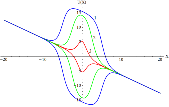
Figure 1: (Colour online) The potential $U(X)$ [Eq. (20)] created by the impurity with $\rho=10$ (blue, 1), $\rho=5$ (green, 2), and $\rho=1$ (red, 3). Other parameters are: $\gamma=0.1,\leavevmode\nobreak\ \mu=\pm 0.25$ and $l=0.1$.

For $\sigma=1$ both extrema lie on the negative half-axis with $X_{min}=X_{+}$, $X_{max}=X_{-}$, while for $\sigma<0$ they lie on the positive half-axis: $X_{min}=X_{-}$, $X_{max}=X_{+}$. It is easy to see that the extrema of potential $U(X)$ are symmetric with respect to the transform $\sigma\to-\sigma$, $X_{max,min}\to-X_{min,max}$. In other words, when the polarity of the impurity changes, the maximum changes sign and becomes the minimum, or vice versa.

In the limiting case $\rho=0,l\to 0\leavevmode\nobreak\ (h\to 1/l^{2})$ the expression for the potential can be obtained explicitly:

$$U(X)=U_{0}(X)-2\pi\gamma X=2\sigma|\mu|\leavevmode\nobreak\ \text{sech}X-2\pi\gamma X\leavevmode\nobreak\ .$$ (22)

The extrema of the potential (22) are given by the following expression

$$X_{\pm}=\sigma\mbox{arcsinh}\left(\frac{|\mu|}{2\pi\gamma}\pm\sqrt{\left(\frac{|\mu|}{2\pi\gamma}\right)^{2}-1}\right)\approx$$ (23)

$$\approx\sigma\left\{\begin{array}[]{c}\frac{\pi\gamma}{|\mu|}\leavevmode\nobreak\ (-)\\ \ln\frac{2|\mu|}{\pi\gamma}\leavevmode\nobreak\ (+)\end{array}\right.,\leavevmode\nobreak\ \leavevmode\nobreak\ \gamma\ll|\mu|\leavevmode\nobreak\ .$$ (26)

4 Threshold current

The current-voltage characteristic (CVC) for the dc-biased LJJ with an impurity usually has a hysteresis-like shape with two characteristic bias values: the critical $\gamma_{c}$ current and the threshold current $\gamma_{thr}<\gamma_{c}$ [25]. The former depends solely on the shape of the potential $U(X)$, and can be easily obtained as a condition for $U(X)$ to have a local minimum. For the current problem it can be derived from positiveness of the expression under the square root in Eq. (16). The threshold current is the minimal current that is needed for a fluxon to pass the obstacle. In other words, at this value of the bias current the LJJ CVC switches from the resistive to the superconducting branch. The threshold current depends not only on the impurity parameters but on the dissipation as well. In this Section we will focus on finding this current for different values of the impurity polarity $\sigma$. The method, developed previously in [28] will be used. The main idea of the method comes from the approximate integration of the newtonian equation of motion for the fluxon center of mass (19)-(20). The left and right sides of this equation can be multiplied by $\dot{X}$ and integrated with respect to time along the interval $t\in[0,t_{stop}]$, where $t_{stop}$ is the time moment when the fluxon stops. Assume that at $t=0$ the fluxon is launched at $X=-\infty$ with kinetic energy $E_{k}$. If the bias is exactly the threshold bias $\gamma_{thr}$, the fluxon will stop at the maximum of $U(X)$ at $X_{max}=X(t_{stop})$. Then, the integration $\int_{0}^{t_{stop}}[\ldots]dt$ of the both sides of the equation of motion is equivalent to the integration $\int_{-\infty}^{X_{max}}[\ldots]dX$ and the threshold current should satisfy the following equation

$$E_{k}+8\alpha\int_{-\infty}^{X_{max}}\left(\frac{\pi\gamma_{thr}}{4\alpha}-\dot{X}\right)dX=U_{0}(X_{max}),$$ (27)

where the fluxon kinetic energy $E_{k}$ and its velocity $v_{\infty}$ at the infinite distance away from the impurity $v_{\infty}$ (see Ref. [25]) are

$${E}_{k}=8\left[(1-v_{\infty}^{2})^{-1/2}-1\right]\simeq 4v_{\infty}^{2}+{\cal O}(v_{\infty}^{4}),\leavevmode\nobreak\$$ (28)

$$v_{\infty}=\left[1+\left(\frac{4\alpha}{\pi\gamma}\right)^{2}\right]^{-1/2}\simeq\frac{\pi\gamma}{4\alpha}+{\cal O}\left[\left(\frac{\pi\gamma}{4\alpha}\right)^{2}\right]\leavevmode\nobreak\ .$$ (29)

The equation (27) can be treated as the energy balance equation $E_{k}+\Delta E=U(X_{max})$ . For the case $\sigma=1$ it has the following physical interpretation: the fluxon kinetic energy $E_{k}$ at the starting point at $X\to-\infty$ is spent on surmounting the local barrier of $U(X)$ and overcoming the dissipation effects (given by the term $\Delta E$). For the case $\sigma=-1$ such an interpretation is not possible because the fluxon receives additional acceleration before starting to climb the barrier.

4.1 Positive polarity case, $\sigma=1$

First we consider the case of positive polarity ($\sigma=1$) for which the dissipative energy loss equals

$$\Delta E=8\alpha\int_{-\infty}^{X_{max}}\left(v_{\infty}-\dot{X}\right)dX\leavevmode\nobreak\ .$$ (30)

We will consider the limit where $\gamma\ll\mu$, $\alpha\ll\mu$. Then, the kinetic energy of the fluxon will take the form: $E_{k}=4v_{\infty}^{2}\approx\left({\pi\gamma}/{2\alpha}\right)^{2}$. In the lowest order of approximation the threshold current can be calculated by equating the fluxon kinetic energy to the maximum height of the potential barrier: $4v_{\infty}^{2}=2{\mu}$, $\gamma_{thr}^{(0)}=2\alpha\sqrt{2\mu}/\pi$. On the other hand, the fluxon kinetic energy satisfies the following $4\dot{X}^{2}=4v_{\infty}^{2}-U(X)$ (the dissipative effects are neglected at this point). After substituting the potential ${U}(X)$ from (22) we will find

$$\dot{X}^{2}=\pi\gamma X/2+\frac{\mu}{2}(1-\text{sech}X)\approx\frac{\mu}{2}(1-\text{sech}X)\leavevmode\nobreak\ .$$ (31)

Now, having the explicit form of $\dot{X}$ we can compute the energy losses due to dissipation:

$$\Delta E = 8\alpha\sqrt{\frac{\mu}{2}}\int_{-\infty}^{X_{max}}\left[1-\sqrt{1-\text{sech}X}\right]dX=$$ (32)

$$= 8\alpha\sqrt{\frac{\mu}{2}}\left[2\leavevmode\nobreak\ \mbox{arcsinh}\left(\cosh{X_{max}}\right)+X_{max}-\ln{2}\right]\simeq$$

$$\simeq 8\alpha\sqrt{\frac{\mu}{2}}\left[2\ln\left(\frac{\sqrt{2}+1}{\sqrt{2}}\right)+X_{max}+{\cal O}(X_{max}^{2})\right]\leavevmode\nobreak\ ,$$

where $X_{min}$, $X_{max}$ are the minima and maxima of $U(X)$. In accordance with (23) $X_{min}\simeq-\ln(2\mu/\pi\gamma)$, $X_{max}\simeq-\pi\gamma/\mu$. Substituting these expressions into (32) and using the expansions of terms with the inverse hyperbolic functions to the Taylor series will find the approximate expression for the dissipative energy loss:

$$\Delta E\approx 4\alpha\sqrt{2\mu}\left[\ln\left(\frac{1+\sqrt{2}}{\sqrt{2}}\right)-\frac{\pi\gamma}{\mu}\right]\leavevmode\nobreak\ .$$ (33)

Here we have assumed $|X_{max}|\ll 1$ and, consequently, the terms ${\cal O}(X_{max}^{2})$ have been dropped. Now we can substitute Eqs. (33) and (22) into the energy balance equation (27). Details of the calculation are given in A. The final equation for threshold current reads:

$$\gamma_{thr}=\frac{2\alpha}{\pi}\left[\sqrt{2\mu}-4\alpha\ln\left(\frac{1+\sqrt{2}}{\sqrt{2}}\right)\right]\leavevmode\nobreak\ .$$ (34)

If the terms ${\cal O}(\alpha^{2})$ are ignored we obtain the expression $\gamma_{thr}=\sqrt{8\mu}\alpha/{\pi}$ which can be derived from purely kinematic approach as in [25]. This approach takes into account only the barrier height of the potential $U(X)$ but not its shape. The ${\cal O}(\alpha^{2})$ correction, on the contrary, accounts for the potential shape as it is different from the respective correction for the microshort impurity [28] where $U(X)\propto\cosh^{-2}X$.

4.2 Negative polarity case $\sigma<0$

Now consider the opposite case of negative impurity amplitude $\mu<0$ ($\sigma=-1$). For this case the extrema points are: $X_{max}\simeq\ln(2|\mu|/\pi\gamma)$, $X_{min}\simeq\pi\gamma/|\mu|$. We seek the approximate solution of Eq. (27) under the same assumption $\gamma\ll|\mu|$ and $\alpha\ll|\mu|$. The integral in the l.h.s of this equation is negative from the moment of the soliton launch till it passes the minimum of $U(X)$ because the fluxon moves down the well, and, therefore, accelerates with respect to the equilibrium velocity $v_{\infty}$. After passing the minimum point it starts to slow down, and, eventually stops at $X=X_{max}$ if $\gamma=\gamma_{thr}$. The largest contribution to the integral in the l.h.s of this equation comes from the area $-1<X<1$ when the fluxon moves around the minimum and has the largest velocity. Here we can assume that it moves according to the equation of motion $4\dot{X}^{2}+U_{0}(X)\approx 0$, and, therefore $X(t)\simeq\sqrt{|\mu|/2}\sqrt{\mbox{sech}X}$. We substitute this law of motion into the main equation (27). As a result we get

$$8\alpha\int_{-\infty}^{X_{max}}(\dot{X}-v_{\infty})dX\simeq$$

$$\simeq 8\left\{\alpha\sqrt{|\mu|}\leavevmode\nobreak\ {}_{2}F_{1}\left[{1\over 4},{1\over 2},{5\over 4},-\left(\frac{\pi\gamma}{2|\mu|}\right)^{2}\right]+\frac{\pi\gamma}{2}\left(1+\ln\frac{\pi\gamma}{2|\mu|}\right)\right\},$$ (35)

where ${}_{2}F_{1}(a,b,c,d)$ is the hypergeometric function [27]. The last term in Eq. (27) equals

$$U_{0}(X_{max})=-4|\mu|\frac{\frac{\pi\gamma}{2|\mu|}}{1+\left(\frac{\pi\gamma}{2\mu}\right)^{2}}\simeq-2\pi\gamma+{\cal O}\left[\left(\frac{\pi\gamma}{2\mu}\right)^{2}\right].$$ (36)

Finally, after some calculations which are presented in A we obtain the final formula for the threshold current:

$$\gamma_{thr}=\frac{4}{\pi^{5/4}}\Gamma\left(\frac{1}{4}\right)|\mu|^{1/4}\alpha^{3/2}+12\frac{\alpha^{2}}{\pi}\ln\left[\left(\frac{2\Gamma\left(\frac{1}{4}\right)}{\pi^{1/4}}\right)^{2/3}\frac{\alpha}{|\mu|^{1/2}}\right]\leavevmode\nobreak\ ,$$ (37)

where $\Gamma(x)$ is the gamma-function. This formula has a structure similar to the expression for $\gamma_{thr}$ for the microresistor [28]. For example, it does not have the ${\cal O}(\alpha)$ term and there is a ${\cal O}(\alpha^{3/2})$ term, which is the lowest order approximation.

4.3 Threshold current for arbitrary values of $\rho$ and $l$.

When the size parameters of the impurity, $l$ and $\rho$, are non-zero it is not possible to obtain the threshold current analytically. Thus, we have used numerical integration of the equations of motion (10-11). For this purpose we have used the 4th order Runge-Kutta method. The polylogarithm function was computed with the help of the CHAPLIN library [29]. In order to be able to get to the $\delta^{\prime}(x)$ limit we have assumed $h=1/l^{2}$ throughout this and next Sections. The numerically calculated threshold current values are presented in Figs. 2-4.

Consider first Fig. 2, where the threshold current dependence on the impurity length $\rho$ is presented. It appears that the difference between $\gamma_{thr}$ for the impurities with different polarities is not significant for small $\rho$’s but increases as $\rho$ increases. Threshold current for $\sigma=1$ ($\mu>0$) is always larger than for $\sigma=-1$. This can be understood from the following argument. For $\sigma=-1$ the fluxon accelerates all the way before the moment when it starts to climb the barrier. For $\sigma=+1$ it slightly decelerates below the equilibrium velocity $v_{\infty}$. Thus, in the $\sigma=-1$ case it needs less energy to overcome the barrier of the same hight as compared with the $\sigma=1$ case. For larger values of $|\mu|$ the difference between $\gamma_{thr}$ for $\sigma=\pm 1$ is more pronounced, while it can be negligible if $|\mu|$ significantly decreases. The same occurs as $l$ is decreased (see Fig. 2b). It should be noted that the impurity height is $h=1/l^{2}$, thus, decrease of $l$ in fact brings the effective increase of $|\mu|$.

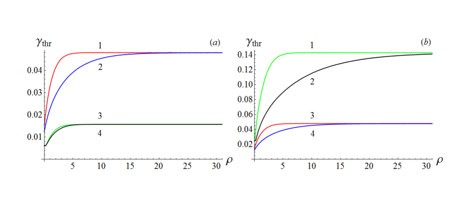
Figure 2: (Colour online) (a) Dependence of the threshold current on the impurity length $\rho$ for different values of $\mu$. For all curves $\alpha=0.1,\leavevmode\nobreak\ l=0.5$; $\mu=0.1$ (1,red), $\mu=-0.1$ (2, blue), $\mu=0.025$ (3, green), $\mu=-0.025$ (4, black). (b) Dependence of the threshold current on $\rho$ and $l$. For all curves $\alpha=0.1$; $\mu=0.1,\leavevmode\nobreak\ l=0.1$ (1, green), $\mu=-0.1,\leavevmode\nobreak\ l=0.1$ (2, black), $\mu=0.1,\leavevmode\nobreak\ l=0.5$ (3, red), $\mu=-0.1,\leavevmode\nobreak\ l=0.5$ (4, blue).

It is interesting to discuss the limit of very long impurities, when the distance between the extremal points of the impurity is large: $\rho\gg 1$. In this case the threshold current should converge to the same value for both polarities as can be observed in Fig. 2. Indeed, if $\sigma=1$, the fluxon approaches the impurity with the velocity $v_{\infty}$ and it should be sufficient enough to overcome the barrier $\Delta U=U(X_{min})-U(X_{max})$. After it has climbed atop the barrier, the fluxon begins to slide down with the velocity which is almost the equilibrium velocity $v_{\infty}$ because the slope of the barrier is defined only by the bias value $\gamma$. If $\sigma=-1$ and the well is very wide, the fluxon falls into the potential well and begins to move there again with the equilibrium velocity $v_{\infty}$. Thus, it approaches the barrier with the equilibrium velocity and need to overcome the barrier of the same height $\Delta U=U(X_{min})-U(X_{max})$. Therefore, the threshold current without the dissipative corrections reads

$$\gamma_{thr}=\frac{2\alpha}{\pi}\sqrt{U(X_{min})-U(X_{max})}\leavevmode\nobreak\ .$$ (38)

On the other hand, it is interesting to look at the dependence of threshold current from dissipation parameter which is presented in Fig. 3. For the positive polarity ($\mu>0$ or $\sigma=1$) the dependence is almost linear and has a good agreement of numerical and analytic results. For the opposite case of $\sigma=-1$ the agreement is quite good for small dissipation but as $\alpha$ increases up to $\alpha\sim 0.05$, the discrepancy between Eq. (37) and numerics becomes strong. At some point the second term in (37) becomes positive and the approximation breaks. Thus, the weakest condition for applicability of the expansion is $\alpha^{2}<\mu$.

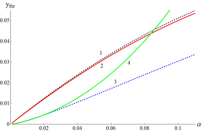
Figure 3: (Colour online) Dependence of the threshold current on $\alpha$. For all curves $\rho=0,\leavevmode\nobreak\ \mu=0.5,\leavevmode\nobreak\ l=0.001$. Dashed curves 1 (black) and 3 (blue) represent the numerical results for $\sigma=1$ and $\sigma=-1$, respectively. Solid curves 2 (red) and 4 (green) show the analytical results (34) and (37), for $\sigma=1$ and $\sigma=-1$ respectively.

Finally, we discuss the dependence of the threshold current on the impurity amplitude $\mu$. The respective dependences are given in Fig. 4. For the positive polarity ($\sigma=1$) the threshold current increases with $\mu$. This is quite natural, because the potential barrier hight increases. The analytical approximation (solid lines) works well in comparison with the numerical data (dashed lines) for all $\mu$’s except the very small ones. The difference between the numerical and analytical results decreases as the ratio $\alpha^{2}/\mu$ decreases. In the limit $\mu\to 0$ the analytical approximation (34) breaks down because the second (negative) term becomes larger than the first one. This happens because this approximation is valid only under the condition $\alpha^{2}\ll\mu$. We have stopped the computation of $\gamma_{thr}$ for the very small values of $\mu$ because it required large junction length and long calculation times.

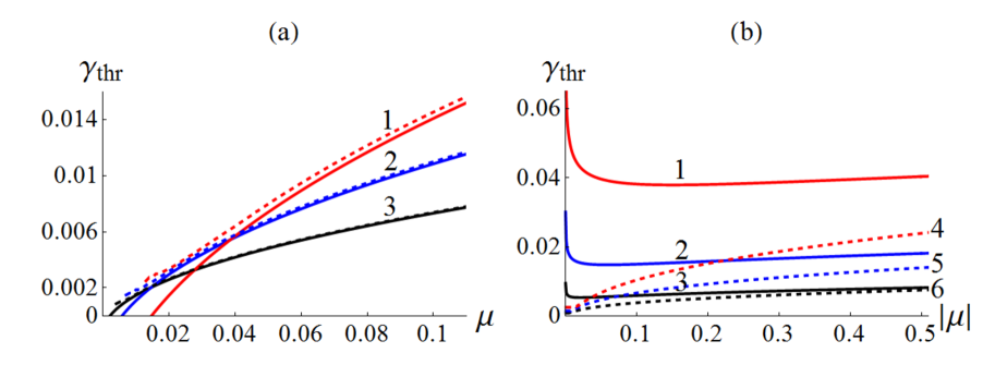
Figure 4: (Colour online) Dependence of the threshold current on the impurity amplitude $\mu$ for $\rho=0$, $\sigma=1$ (a) and $\sigma=-1$ (b). Numerically computed results are shown by the dashed lines and the solid lines correspond to Eqs. (34) and (37). The dissipation values are $\alpha=0.08$ (curve 1, red), $\alpha=0.05$ (curve 2, blue) and $\alpha=0.03$ (curve 3, black). The dashed curves in (b) correspond to $\alpha=0.08$ (curve 4, red), $\alpha=0.05$ (curve 5, blue) and $\alpha=0.03$ (curve 6, black).

In the negative polarity case $\sigma=-1$ we observe the non-physical divergence of the $\gamma_{thr}(|\mu|)$ dependence [see Fig. 4(b)]. It occurs again due to the fact that the analytical approximation is not valid if $\mu\ll\alpha^{2}$. On the other hand, we observe the convergence of the numerically computed (dashed) results with the analytical approximation Eq. (37) (solid lines) as $|\mu|$ increases. We remind once again that this approximation works only if $\alpha^{2}\ll|\mu|$. The fastest convergence is observed for the smallest dissipation value, $\alpha=0.03$ (black curves 3 and 6). While for the $\sigma=+1$ case the threshold current increases as $\gamma_{thr}\propto\mu^{1/2}$, for the negative polarity it seems to tend to some constant value. In reality it also increases, but as a $|\mu|^{1/4}$ function, which grows much slower. Our calculations have been performed for $\rho=0$, however, as we know from Fig. 2, the threshold current increases when $\rho$ increases. Therefore, the $\gamma_{thr}(\mu)$ dependence should be modified accordingly for $\rho\neq 0$.

5 Fluxon delay time on the impurity

During its motion along the junction the fluxon meets the impurity and interacts with it, whereupon the fluxon velocity changes. After leaving the impurity the fluxon velocity returns to the equilibrium value $v_{\infty}$. As it was shown in the previous sections, the dynamics of the fluxon transmission through the impurity with different $\sigma$ is quite different. In particular, it takes different amount of time for the fluxon to pass through the $\sigma=1$ and the $\sigma=-1$ impurities, respectively. Thus, it is possible to define the delay time $\Delta t$ as a difference between the time, necessary for the fluxon to pass some fixed distance over the $\sigma=-1$ and $\sigma=+1$ impurities with all other parameters (including $\gamma$) fixed. In [5, 9] the process of the qubit read-out has been proposed. The qubit is coupled to the Josephson transmission line and is described theoretically as a dipole impurity. Its state is defined by the sign of $\sigma$. The delay time can be measured and is used to determine the state of the qubit.

In order to find the delay time we have performed numerical simulations of the fluxon equations of motion (10)-(11). The fluxon is launched at some distant point to the left from the impurity. Next, we measure numerically how much time has passed while fluxon got to the observation point on the right side from the impurity. Then the polarity of the impurity is changed and the same computation is repeated again. The difference between the obtained times is the fluxon delay time $\Delta t$. The absolute value of this delay time depends on the parameters of the impurity and on the initial fluxon velocity $v_{\infty}$, which itself depends on the external bias. The delay time as a function of the initial fluxon velocity is presented in Figs. 5-7 for the different parameters of the impurity.

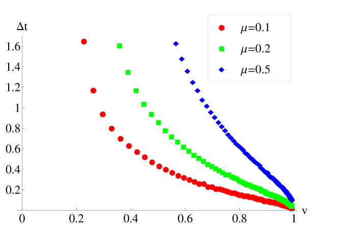
Figure 5: (Colour online) Fluxon delay time as a function of the fluxon velocity for the junction with $\alpha=0.1$ and impurity with $l=0.5,\leavevmode\nobreak\ \rho=0.1$ and different strength $|\mu|$ (shown in the legend box).

The main feature of all these three figures is the fact that the delay time decreases while the fluxon velocity increases and tends to zero as $v\to 1$. This happens because the fluxon energy increases in the relativistic limit as $\propto(1-v^{2})^{-1/2}$, thus, the energy of the impurity-created potential barrier becomes negligible comparing to the fluxon kinetic energy. As a result, there should be no difference in the fluxon transmission through the $\sigma=+1$ and $\sigma=-1$ impurity at $v\to 1$. Also, if the bias current exceeds the critical current, there should be no pinning potential $U(X)$ at all. All the dependencies start from some certain finite value which is defined by the threshold current ${\gamma_{thr}}_{\sigma=+1}$. From Sec. 4 we already know that ${\gamma_{thr}}_{\sigma=+1}>{\gamma_{thr}}_{\sigma=-1}$ for all other parameter values. Therefore, we have performed our computations for the bias $\gamma>{\gamma_{thr}}_{\sigma=+1}$. Calculations for the bias in the interval ${\gamma_{thr}}_{\sigma=-1}<\gamma<{\gamma_{thr}}_{\sigma=+1}$ do not makes sense since $\Delta t$ would be infinity simply because for $\sigma=1$ the fluxon would never arrive at the measurement point. However, it does not mean that the experimental read-out process is not possible for this range. Moreover, in this interval it will be the most efficient.

In Fig. 5 the $\Delta t(v)$ dependence for different values of the impurity amplitude $|\mu|$ is shown. The shape parameters of the impurity, $l$ and $\rho$ [see Eq. (7)] are fixed. The main feature of this graph is that the delay time increases considerably (several times) when the impurity amplitude $|\mu|$ increases. The similar dependence in Fig. 6 manifests that $\Delta t(v)$ increases when the impurity length $\rho$ is increasing but the width of the barrier $l$ is fixed. We observe that the total impurity length influences the delay time.

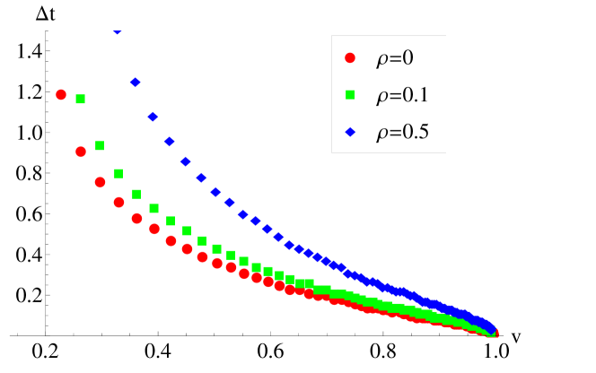
Figure 6: (Colour online) Fluxon delay time as a function of its velocity for the junction with $\alpha=0.1$ and impurity with $l=0.5,\leavevmode\nobreak\ |\mu|=0.1$ and different length $\rho$ (shown in the legend box).

If $\rho$ is increased, the delay time increases as well and this increase can be up to factor two. When the change of $l$ is concerned, the delay time is much less sensitive to the change of this parameter. In Fig. 7 we observe that there is no visible change in $\Delta t$ when $l$ is increased from $l=0.001$ to $l=0.1$. If one considers a quite moderate change of $\rho$ from $0$ to $0.1$

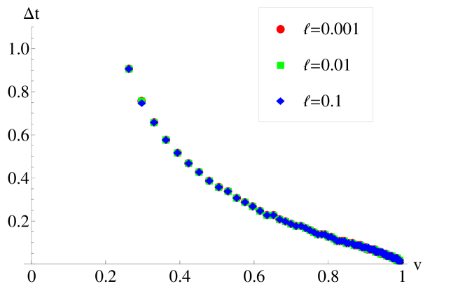
Figure 7: (Colour online) Fluxon delay time as a function of its velocity for the junction with $\alpha=0.1$ and impurity with $\rho=0,\leavevmode\nobreak\ |\mu|=0.1$ and different values of $l$ (shown in the legend box).

in Fig. 6 (compare red and green markers), the increase of $\Delta t$ is small but is still clearly visible. The very weak dependence on the parameter $l$ is explained by the fact that the height of the barrier equals $h=1/l^{2}$ and the impurity amplitude $\mu$ is multiplied by this coefficient [see Eqs. (10)-(11)]. Thus, the increase of the impurity length is compensated by the effective decrease of its amplitude. In fact, the parameter $l$ measures the deviation from the $\delta^{\prime}(x)$ approximation. We see that this approximation works fairly well. The parameter $\rho$, on contrary, is not connected to other system parameters and controls the proper width of the potential barrier $U(X)$ that is created by the qubit.

6 Discussion and conclusions

In this paper the fluxon interaction with the dipole-like impurity in the long Josephson junction (LJJ) has been investigated. The problem arises when studying the fluxon-Abrikosov vortex interaction [10, 11] in LJJ and the qubit state read-out process [5, 7, 9] in the Josephson transmission line coupled to the qubit. At variance with the previous research we take into account the finite size of the impurity. The impurity is modelled by the piecewise function that contains the well and barrier with the width $l$ each that are separated from each other by the distance $\rho$. The impurity remains antisymmetric and reduces to the $\delta^{\prime}(x)$ function in the limit when the barrier(well) width becomes infinitely small.

The main results of this research can be formulated as follows. The physical size of impurity influences considerably the fluxon-impurity interaction. The most interesting result is the strong dependence of the threshold pinning current on the impurity length, $\rho$. The threshold current increases monotonically as $\rho$ increases, however, this is saturation growth which tends to some constant value of $\gamma_{thr}$. The growth almost stops at some critical value that equals several units of $\lambda_{J}$ (Josephson penetration depth) and depends on the impurity amplitude. There exist an optimal range of $\rho$ for which the difference between ${\gamma_{thr}}_{\sigma=-1}$ and ${\gamma_{thr}}_{\sigma=+1}$ is maximal. Thus, the range for the external bias where the ${\gamma_{thr}}_{\sigma=-1}<\gamma<{\gamma_{thr}}_{\sigma=+1}$ can be increased considerably if $\rho$ and/or the impurity amplitude $\mu$ are chosen appropriately. In this range the qubit read-out process is the most efficient because the fluxon will not pass the qubit with $\sigma=1$. The fluxon delay time (the difference between the times necessary to pass the $\sigma=1$ and $\sigma=-1$ qubits) depends on the impurity length $\rho$, its amplitude $\mu$ and is almost independent on the impurity barrier width $l$. There is an important difference between the parameters $l$ and $\rho$. The parameter $l$ also enters as the $1/l^{2}$ prefactor before the amplitude $\mu$ in the equations of motion. Therefore, it can be treated as a measure of the deviation from the $\delta^{\prime}(x)$ limit. From the obtained results we conclude that the piece-wise approximation of the $\delta^{\prime}(x)$ impurity works well. On the contrary, the parameter $\rho$ influences only the length of the impurity and not its amplitude.

As far as the future research is concerned, we believe that consideration of the two-dimensional JJ is important alongside with the studies of the Josephson plasmon radiation due to fluxon scattering on such a finite-size dipole impurity for both the 1D and 2D Josephson junctions.

Appendix A Correction calculation

In this Appendix the details on how the second order correction for $\gamma_{thr}$ is calculated.

Case $\sigma=1$ ($\mu>0$)

Taking to account that $\text{sech}(-\pi\gamma/\mu)=1-\pi^{2}\gamma^{2}/2\mu^{2}$ and Eq. (32) we can rewrite the energy balance equation:

$$\left(\frac{\pi\gamma}{2\alpha}\right)^{2}+8\alpha\sqrt{\frac{\mu}{2}}\left[2\ln\left(\frac{1+\sqrt{2}}{\sqrt{2}}\right)-\frac{\pi\gamma}{\mu}\right]=2\mu\left[1-\frac{1}{2}\left(\frac{\pi\gamma}{\mu}\right)^{2}\right]\leavevmode\nobreak\ .$$ (39)

We introduce the following small parameters:

$$G=\frac{\pi\gamma}{2|\mu|}\ll 1,\leavevmode\nobreak\ \leavevmode\nobreak\ \Upsilon=\alpha\sqrt{\frac{2}{|\mu|}}\ll 1\leavevmode\nobreak\ .$$ (40)

As a result, we get a nonlinear algebraic equation

$$\left(\frac{G}{\Upsilon}\right)^{2}=-4\Upsilon\left[\ln\left(\frac{1+\sqrt{2}}{\sqrt{2}}\right)-G\right]+1,$$ (41)

where the terms of the order ${\cal O}(\Upsilon^{2})$,${\cal O}(G^{2})$ and higher have been neglected in the right hand side. It is easy to see that in the lowest order the following equality holds: $\Upsilon=G$. Thus, if we want to obtain the second order correction we look for the small correction to the above formula: $G=\Upsilon+\Delta\Upsilon$, $\Delta\Upsilon\ll\Upsilon,G$. Substitution of this expansion in Eq. (41) yields

$$\Delta\Upsilon+2\ln\left(\frac{1+\sqrt{2}}{\sqrt{2}}\right)\Upsilon^{2}=0,$$ (42)

where the terms ${\cal O}(\Upsilon^{3})$ and higher have been neglected. As a result the final expression for the threshold current reads:

$$G=\Upsilon\left[1-\Upsilon\ln\left(\frac{1+\sqrt{2}}{\sqrt{2}}\right)\right],$$ (43)

or

$$\gamma_{thr}=\frac{2\alpha}{\pi}\left[\sqrt{2\mu}-4\alpha\ln\left(\frac{1+\sqrt{2}}{\sqrt{2}}\right)\right]\leavevmode\nobreak\ .$$ (44)

Case $\sigma=-1(\mu<0)$

The energy balance equation [see Eq. (35)] reads:

$$\left(\frac{\pi\gamma}{2\alpha}\right)^{2}=8\left\{\alpha\sqrt{\mu}\leavevmode\nobreak\ {}_{2}F_{1}\left[{1\over 4},{1\over 2},{5\over 4},-\left(\frac{\pi\gamma}{2\mu}\right)^{2}\right]+\frac{\pi\gamma}{2}\left(1+\ln\frac{\pi\gamma}{2\mu}\right)\right\}-2\pi\gamma\leavevmode\nobreak\ .$$ (45)

We introduce parameters $G$ and $\Upsilon$ in the same way as in Eqs. (40):

$$\left(\frac{G}{\Upsilon}\right)^{2}=4\sqrt{2}\frac{\Upsilon}{\sqrt{G}}\leavevmode\nobreak\ {}_{2}F_{1}\left({1\over 4},{1\over 2},{5\over 4},-\frac{1}{G^{2}}\right)+4G\ln{G}\leavevmode\nobreak\ .$$ (46)

With the help of the transformation formulae for the hypergeometric function [27] we can rewrite the function with its fourth variable becoming $-G^{2}$. After that it can be expanded in the Taylor series up to the term ${\cal O}(G^{2})$:

$${}_{2}F_{1}\left({1\over 4},{1\over 2},{5\over 4},-\frac{1}{G^{2}}\right)=\frac{1}{4}\Gamma^{2}\left(\frac{1}{4}\right)\left[\sqrt{\frac{G}{\pi}}{}_{2}F_{1}\left({1\over 4},0,{3\over 4},-G^{2}\right)+\right.$$ (47)

$$\left.+\frac{1}{\sqrt{2}\pi}{}_{2}F_{1}\left({1\over 2},{1\over 4},{5\over 4},-G^{2}\right)\right]\simeq\frac{1}{4}\Gamma^{2}\left(\frac{1}{4}\right)\left(\sqrt{\frac{G}{\pi}}+\frac{G}{\sqrt{2}\pi}\right)\leavevmode\nobreak\ ,$$

where $\Gamma(x)$ is the gamma function. Taking into account that both $G$ and $\Upsilon$ are small parameters, we can rewrite Eq. (46) as

$$G\simeq G_{0}+G_{1}=\left(\frac{2}{\pi}\right)^{1/4}\Gamma\left(\frac{1}{4}\right)\Upsilon^{3/2}+G_{1},\leavevmode\nobreak\ \leavevmode\nobreak\ G_{1}\ll G_{0}\leavevmode\nobreak\ .$$ (48)

In the zero approximation, $G\simeq G_{0}$ we obtain

$$\gamma_{thr}^{(0)}=\frac{4}{\pi^{5/4}}\Gamma\left(\frac{1}{4}\right)|\mu|^{1/4}\alpha^{3/2}\leavevmode\nobreak\ .$$ (49)

Substitution of the expansion (48) into (46) yields the correction term $G_{1}$,

$$G_{1}=2\Upsilon^{2}\ln\left[\left(\frac{2}{\pi}\right)^{1/4}\Gamma\left(\frac{1}{4}\right)\Upsilon^{3/2}\right]\leavevmode\nobreak\ .$$ (50)

As a result, we get the full expression for the threshold current:

$$\gamma_{thr}=\frac{4}{\pi^{5/4}}\Gamma\left(\frac{1}{4}\right)|\mu|^{1/4}\alpha^{3/2}+12\frac{\alpha^{2}}{\pi}\ln\left[\left(\frac{2\Gamma\left(\frac{1}{4}\right)}{\pi^{1/4}}\right)^{2/3}\frac{\alpha}{|\mu|^{1/2}}\right]\leavevmode\nobreak\ .$$ (51)

References

- [1] A. Barone, G. Paterno, Physics and Applications of the Josephson Effect, Wiley, New York, 1982.
- [2] A. V. Ustinov, Solitons in Josephson junctions, Physica D 123 (1-4) (1998) 315–329.
- [3] V. P. Koshelets, S. V. Shitov, Integrated superconducting receivers, Superconductor Science and Technology 13 (5) (2000) R53–R70.
- [4] A. Kemp, A. Wallraff, A. Ustinov, Josephson vortex qubit: Design, preparation and read-out, physica status solidi (b) 233 (3) (2002) 472–481.
- [5] D. V. Averin, K. Rabenstein, V. K. Semenov, Rapid ballistic readout for flux qubits, Phys. Rev. B 73 (2006) 094504.
- [6] A. N. Price, A. Kemp, D. R. Gulevich, F. V. Kusmartsev, A. V. Ustinov, Vortex qubit based on an annular Josephson junction containing a microshort, Phys. Rev. B 81 (2010) 014506.
- [7] K. G. Fedorov, A. V. Shcherbakova, R. Schäfer, A. V. Ustinov, Josephson vortex coupled to a flux qubit, Appl. Phys. Lett. 102 (2013) 132602.
- [8] K. G. Fedorov, A. V. Shcherbakova, M. J. Wolf, D. Beckmann, A. V. Ustinov, Fluxon readout of a superconducting qubit, Phys. Rev. Lett. 112 (2014) 160502.
- [9] A. Fedorov, A. Shnirman, G. Schön, A. Kidiyarova-Shevchenko, Reading out the state of a flux qubit by Josephson transmission line solitons, Phys. Rev. B 75 (22) (2007) 224504.
- [10] L. G. Aslamazov, E. V. Gurovich, Pinning of solitons by Abrikosov vortices in distributed Josephson junctions, JETP Lett. 40 (1984) 746–749.
- [11] M. V. Fistul, G. F. Giuliani, Abrikosov vortices in long Josephson junctions, Phys. Rev. B 58 (1998) 9348–9353.
- [12] B. A. Malomed, A. V. Ustinov, Creation of classical and quantum fluxons by a current dipole in a long Josephson junction, Phys. Rev. B 69 (2004) 064502.
- [13] P. Šeba, Some remarks on the -interaction in one dimension, Reports on Mathematical Physics 24 (1) (1986) 111–120.
- [14] P. Kurasov, Distribution theory for discontinuous test functions and differential operators with generalized coefficients, Journal of Mathematical Analysis and Applications 201 (1996) 297–323.
- [15] P. L. Christiansen, H. C. Arnbak, A. V. Zolotaryuk, V. N. Ermakov, Y. B. Gaididei, On the existence of resonances in the transmission probability for interactions arising from derivatives of Dirac’s delta function, Journal of Physics A: Mathematical and General 36 (27) (2003) 7589–7600.
- [16] Y. D. Golovaty, S. S. Man’ko, Solvable models for the schrödinger operators with -like potentials, Ukr. Math. Bull 6 (2009) 169–203.
- [17] Y. D. Golovaty, R. O. Hryniv, On norm resolvent convergence of schrödinger operators with -like potentials, Journal of Physics A: Mathematical and Theoretical 43 (15) (2010) 155204; Y. D. Golovaty, R. O. Hryniv, On norm resolvent convergence of schrödinger operators with -like potentials, Journal of Physics A: Mathematical and Theoretical 44 (4) (2011) 049802.
- [18] A. V. Zolotaryuk, P. L. Christiansen, S. V. Iermakova, Scattering properties of point dipole interactions, Journal of Physics A: Mathematical and General 39 (29) (2006) 9329–9338.
- [19] A. V. Zolotaryuk, Y. Zolotaryuk, Intrinsic resonant tunneling properties of the one-dimensional schrÖdinger operator with a delta derivative potential, Int. J. Mod. Phys. B 28 (01) (2014) 1350203.
- [20] Y. S. Kivshar, A. M. Kosevich, O. A. Chubykalo, Finite-size effects in fluxon scattering by an inhomogeneity, Phys. Lett. A 129 (1988) 449–452.
- [21] G. Derks, A. Doelman, C. J. K. Knight, H. Susanto, Pinned fluxons in a Josephson junction with a finite-length inhomogeneity, European Journal of Applied Mathematics 23 (2) (2012) 201–244.
- [22] B. A. Malomed, Dynamics of quasi-one-dimensional kinks in the two-dimensional sine-Gordon model, Physica D: Nonlinear Phenomena 52 (1991) 157 – 170.
- [23] I. O. Starodub, Y. Zolotaryuk, Fluxon scattering on a stripe-like impurity in a two-dimensional Josephson junction, Ukr. J. Phys. 58 (7) (2013) 687–696.
- [24] I. O. Starodub, Y. Zolotaryuk, Radiation emission due to fluxon scattering on an inhomogeneity in a large two-dimensional Josephson junction, Phys. Rev. B 90 (2014) 224509.
- [25] D. W. McLaughlin, A. C. Scott, Perturbation analysis of fluxon dynamics, Phys. Rev. A 18 (4) (1978) 1652–1680.
- [26] J.-L. Gervais, B. Sakita, Extended particles in quantum field theories, Phys. Rev. D 11 (10) (1975) 2943–2945.
- [27] M. Abramowitz, I. Stegun, Pocketbook of Mathematical Functions, Verlag Harri Deutsch, Frankfurt/Main, 1984.
- [28] Y. S. Kivshar, B. A. Malomed, A. A. Nepomnyashchy, Interaction of fluxon with localized inhomogeneity in a long Josephson junction, Sov. Phys. JETP 94 (1988) 356–365.
- [29] CHAPLIN - Complex Harmonic Polylogarithms in FORTRAN, arXiv:1106.5739, https://chaplin.hepforge.org/.