Relaxation Functions of Ornstein-Uhlenbeck Process with Fluctuating Diffusivity

Abstract

We study a relaxation behavior of an Ornstein-Uhlenbeck (OU) process with a time-dependent and fluctuating diffusivity. In this process, the dynamics of a position vector is modeled by the Langevin equation with a linear restoring force and a fluctuating diffusivity (FD). This process can be interpreted as a simple model of the relaxational dynamics with internal degrees of freedom or in a heterogeneous environment. By utilizing the functional integral expression and the transfer matrix method, we show that the relaxation function can be expressed in terms of the eigenvalues and eigenfunctions of the transfer matrix, for general FD processes. We apply our general theory to two simple FD processes, where the FD is described by the Markovian two-state model or an OU type process. We show analytic expressions of the relaxation functions in these models, and their asymptotic forms. We also show that the relaxation behavior of the OU process with an FD is qualitatively different from those obtained from conventional models such as the generalized Langevin equation.

I Introduction

Recently, diffusion of Brownian particles with time-dependent and fluctuating diffusivity has been studied extensively in many contexts such as diffusion in heterogeneous environments and a simple model of normal yet non-Gaussian diffusionChubynsky and Slater (2014); Bressloff and Newby (2014); Bressloff (2016); Massignan et al. (2014); Yamamoto et al. (2014); Manzo et al. (2015); Uneyama et al. (2015); Miyaguchi et al. (2016); Chechkin et al. (2017); Jain and Sebastian (2017); Sergé et al. (2008). (The anomalous diffusion behavior of time-dependent diffusivity models has been also studiedCherstvy and Metzler (2015, 2016).) The Langevin equation with a time-dependent and fluctuating diffusivity exhibits non-trivial diffusion behavior. If the system is in equilibrium, the ensemble-averaged mean-square displacement (MSD) reduces to just a normal diffusion which is the same as the simple Brownian motion. However, this does not mean that the diffusion behavior can be expressed as a normal and Gaussian process. If we consider the (time-averaged) MSD data for individual realizations, the distribution of MSD data around their ensemble-average does not obey the Gaussian distribution. This is because the thermal noise becomes non-Gaussian due to the multiplicative coupling between the fluctuating diffusivity (FD) and the Gaussian noise. The non-Gaussian nature becomes evident if we consider the higher order correlation functions. For example, the authors showed that the relative standard deviation of the time-averaged MSD (the square of which is also known as the ergodicity breaking parameterHe et al. (2008); Cherstvy et al. (2013)) can be related to the correlation function of an FDUneyama et al. (2015).

The concept of the FD seems to be useful to study the microscopic dynamical behavior of molecules with the internal degrees of freedom and/or in heterogeneous environments. For example, protein dynamics has many internal degrees of freedom and the conformational dynamics exhibits non-single-exponential type relaxation behaviorYang et al. (2003); Yamamoto et al. (2014); Hu et al. (2015). The diffusivity of the center of mass of an entangled polymer depends on the end-to-end vector of the polymer chainDoi and Edwards (1978, 1986); Uneyama et al. (2015). A molecule in a supercooled liquids exhibits heterogeneous and fluctuating diffusion behavior, which is known as the dynamic heterogeneityYamamoto and Onuki (1998a, b); Sillescu (1999). We expect that other dynamical behavior, such as the relaxation behavior, in these systems reflects their FDs.

Unfortunately, from the view point of experiments, the direct observations of MSDs of individual molecules are not easy in some systems. Instead of the direct observations of individual molecules, the macroscopic measurements of relaxation functions (response functions) are useful. The macroscopic relaxation functions can be measured by imposing an external perturbation to the system and monitoring the response of the system. The linear response theory gives the relation between the time-correlation function of microscopic variables and the macroscopic response functionEvans and Morris (2008). Thus we can study the microscopic molecular-level dynamics from the macroscopic response functions. For example, we can investigate microscopic molecular dynamics of polymers from the experimental data of the dielectric relaxation function (the response function of the electric flux to the imposed electric field) and the relaxation modulus (the response function of the stress to the imposed strain)Watanabe (1999); Matsumiya et al. (2011).

At the molecular-level, we expect that relaxation dynamics can be described by a Langevin equation with a restoring force. The Ornstein-Uhlenbeck (OU) processvan Kampen (2007) is the simplest model to describe such dynamics. For example, in the harmonic dumbbell model for a polymer, the dynamics is described as an OU type process. Dynamics of a colloidal particle under an optical tweezer can also be modeled as an OU type process. If a molecule or a particle is in a heterogeneous environment (such as a supercooled liquid), we expect that the relaxation behavior is affected by an FD arising from the heterogeneity. The relaxation behavior of a polymer or a colloidal particle in a supercooled environment will be affected both by a restoring force and a heterogeneous environment. Dynamics of a protein may also be interpreted as relaxation dynamics under a heterogeneous environment.

Thus we expect that the relaxation behavior of the systems with FDs would be informative to model and/or analyze microscopic molecular dynamics of polymers and supercooled liquids. However, the relaxation behavior of the Langevin equation with an FD has not been studied in detail, as far as the authors know. In this work, we consider an OU type process with a time-dependent and fluctuating diffusivity as a simple and analytically tractable relaxation model with an FD. We theoretically analyze relaxation functions and show that the relaxation functions are strongly affected by the dynamics of the diffusivity. We give a formal expression for the relaxation function for a general Markovian dynamics of diffusivity. We show that the form of the relaxation function is determined as a result of the competition between the relaxation (diffusion) dynamics in the OU process and the transition dynamics of the FD. Then we apply our result to two simple and solvable models. One is the Markovian two-state model where the diffusivity can take only two different values. Another is the OU type model where the noise coefficient obeys an OU process. We discuss the properties of the relaxation functions by the OU process with an FD, and possible applications of our theoretical results to the analyses of experimental data.

II Model

We consider the dynamics of a position in a $d$-dimensional space, $\bm{r}$. This position can be interpreted as the position of a tagged particle in the system, or a bond vector which connects two particles (in the dumbbell modelKröger (2004)). In both cases, at the mesoscopic scale, the dynamics of the position can be reasonably described by the Langevin type equation. We consider the dynamics of a particle or a bond vector in a heterogeneous environment, where the diffusivity (or the mobility) fluctuates in time. The effect of the inertia term in a dynamic equation is generally small at the mesoscopic scale, and thus we can safely ignore the inertial term (the overdamped limit). As a simple model to describe such systems, we employ the Langevin equation with an FDUneyama et al. (2015):

$$\frac{d\bm{r}(t)}{dt}=\frac{D(t)}{k_{B}T}\bm{F}(\bm{r},t)+\sqrt{2D(t)}\bm{w}(t).$$ (1)

Here, $k_{B}$ is the Boltzmann constant, $T$ is the temperature, $D(t)$ is a time-dependent and fluctuating diffusivity, $\bm{F}(\bm{r},t)$ is the force for the position, and $\bm{w}(t)$ is the Gaussian white noise. We limited ourselves to the case where the diffusion coefficient is given as a scalar quantity. (In general, the diffusion coefficient is a tensor quantityUneyama et al. (2015); Miyaguchi (2017).) From the fluctuation-dissipation relation of the second kind, the first and second moments of the Gaussian noise $\bm{w}(t)$ are $\langle\bm{w}(t)\rangle=0$ and $\langle\bm{w}(t)\bm{w}(t^{\prime})\rangle=\bm{1}\delta(t-t^{\prime})$, where $\langle\dots\rangle$ represents the statistical average and $\bm{1}$ is the unit tensor in $d$-dimensions. We assume that the dynamics of $D(t)$ is statistically independent of the noise $\bm{w}(t)$. Namely, the dynamics of $D(t)$ is statistically not affected by the dynamics of $\bm{r}(t)$.

Eq (1) can be interpreted as a simplified model for dynamics of supercooled polymer meltsBaschnagel and Varnik (2005); Ding and Sokolov (2006) or trapped Brownian particles in heterogeneous environmentsWong et al. (2004); Shundo et al. (2011); Hori et al. (2012). For the case of a polymer chain in a supercooled melt, we consider the end-to-end vector as the bond vector and the effective potential can be expressed as a harmonic potentialDoi and Edwards (1986). For the case of a trapped Brownian particle, we consider the situation where the Brownian particle is trapped by an optical tweezer. The effective potential by an optical tweezer can be approximated well by a harmonic potentialFlorin et al. (1998). Thus we assume that the force in eq (1) is derived from a harmonic potential $U(\bm{r})=\alpha k_{B}T\bm{r}^{2}/2$, where $\alpha$ is constant. (If the force is purely entropic, $\alpha$ is independent of the temperature $T$Doi and Edwards (1986). However, in general, $\alpha$ depends on the temperature. Fortunately, the explicit form of $\alpha$ and its temperature dependence is not important for the analyses in this work.) The force becomes $\bm{F}=-{\partial U(\bm{r})}/{\partial\bm{r}}=-\alpha k_{B}T\bm{r}$ , and eq (1) reduces to the following OU process with an FD (OUFD):

$$\frac{d\bm{r}(t)}{dt}=-\alpha D(t)\bm{r}(t)+\sqrt{2D(t)}\bm{w}(t).$$ (2)

We show an example of the OUFD process in Figure 1. If $D(t)$ is constant, eq (2) reduces to a usual OU processvan Kampen (2007), and we can easily analyze it. (As clearly observed in Figure 1, the fluctuation of the diffusivity qualitatively affects the stochastic process, and thus generally the OUFD behaves in a different way from a usual OU process.)

To fully describe the OUFD, we need the dynamic equation for $D(t)$. We assume that the dynamics of $D(t)$ obeys a Markovian stochastic process, and $D(t)$ is sampled from the equilibrium ensemble. (The effect of non-equilibrium initial ensembles to the OU process with a constant diffusivity was recently studiedCherstvy et al. (2018).) For example, we can employ a Markovian jump processes between several discrete states for the diffusivity, or a Langevin equation for the diffusivity. In any case, as far as the process is Markovian, we can formally express the time-evolution equation for the probability distribution of $D$ by a master equation as

$$\frac{\partial P(D,t)}{\partial t}=\hat{\mathcal{L}}P(D,t),$$ (3)

where $P(D,t)$ is the probability distribution of $D$ at time $t$, and $\hat{\mathcal{L}}$ is a linear operator (such as the Fokker-Planck operator and the transition matrixvan Kampen (2007)). Or, more generally, we assume that the diffusivity $D(t)$ is obtained from a Markovian variable $\xi(t)$ as $D(t)=D(\xi(t))$, and that its probability distribution follows a master equation

$$\frac{\partial P(\xi,t)}{\partial t}=\hat{\mathcal{L}}P(\xi,t).$$ (4)

Note that Eq. (3) is a special case for which $D(t)=\xi(t)$.

To study the relaxational behavior of the OU process, we consider the following relaxation function:

$$\Phi(t)\equiv\frac{\langle\bm{r}(t)\cdot\bm{r}(0)\rangle}{\langle\bm{r}^{2}(0)\rangle}.$$ (5)

Here, it should be noticed that the statistical average $\langle\dots\rangle$ is taken both for the noise $\bm{w}(t)$ and the diffusion coefficient $D(t)$. In this work, we take the statistical average of $\bm{w}(t)$ before that of $D(t)$. The order of two statistical avareges does not affect the results in most cases, including the equilibrium systems. Eq (5) can be interpreted as the normalized relaxation function of $\bm{r}(t)$. If we interpret $\bm{r}(t)$ as the bond vector and it has an electric dipole, eq (5) can be related to the dielectric relaxation functionWatanabe (1999). If we interpret $\bm{r}(t)$ as the position of a trapped particle, eq (5) can be related to the ensemble-averaged MSD as

$$\langle[\bm{r}(t)-\bm{r}(0)]^{2}\rangle=2\langle\bm{r}^{2}(0)\rangle[1-\Phi(t)].$$ (6)

Therefore, if the relaxation function $\Phi(t)$ exhibits some non-trivial properties, we will observe them via the ensemble-averaged MSD. This is in contrast to the case without a trap potential, where the ensemble-averaged MSD exhibits just a normal diffusion.

We calculate the relaxation function $\Phi(t)$ for the OUFD, from eq (2) and (5). By integrating eq (2) from time $0$ to $t$, we have

$$\begin{split}\bm{r}(t)&=\exp\left[-\alpha\int_{0}^{t}dt^{\prime}\,D(t^{\prime})\right]\bm{r}(0)\\ &\qquad+\int_{0}^{t}dt^{\prime}\exp\left[-\alpha\int_{t^{\prime}}^{t}dt^{\prime\prime}\,D(t^{\prime\prime})\right]\sqrt{2D(t^{\prime})}\bm{w}(t^{\prime}).\end{split}$$ (7)

Because $D(t)$, $\bm{w}(t)$ (for $t>0$) and $\bm{r}(0)$ are statistically independent of each other, we take the average over $\bm{w}(t)$ and $\bm{r}(0)$. Then we have

$$\langle\bm{r}(t)\cdot\bm{r}(0)\rangle=\left\langle\exp\left[-\alpha\int_{0}^{t}dt^{\prime}\,D(t^{\prime})\right]\right\rangle\langle\bm{r}^{2}(0)\rangle,$$ (8)

and

$$\Phi(t)=\left\langle\exp\left[-\alpha\int_{0}^{t}dt^{\prime}\,D(t^{\prime})\right]\right\rangle.$$ (9)

For comparison, we also consider another relaxation function defined as

$$\Psi(t)\equiv\frac{\langle[r_{x}(t)r_{y}(t)][r_{x}(0)r_{y}(0)]\rangle}{\langle[r_{x}(0)r_{y}(0)]^{2}\rangle}.$$ (10)

We have assumed that the dimension of the space is at least $2$ ($d\geq 2$). Eq (10) can be interpreted as the normalized relaxation function of the off-diagonal component of a second rank tensor $\bm{r}(t)\bm{r}(t)$. If we interpret $\bm{r}(t)$ as a bond vector, the relaxation function $\Psi(t)$ can be related to the relaxation modulus (the viscoelastic relaxation function)Watanabe (1999). The relaxation function $\Psi(t)$ can be calculated in a similar way to $\Phi(t)$. From eq (7), we have

$$\langle r_{x}(t)r_{y}(t)r_{x}(0)r_{y}({0})\rangle=\left\langle\exp\left[-2\alpha\int_{0}^{t}dt^{\prime}\,D(t^{\prime})\right]\right\rangle\langle r_{x}^{2}(0)r_{y}^{2}(0)\rangle,$$ (11)

and thus

$$\Psi(t)=\left\langle\exp\left[-2\alpha\int_{0}^{t}dt^{\prime}\,D(t^{\prime})\right]\right\rangle.$$ (12)

If $D(t)$ is constant, $\Psi(t)$ can be related to $\Phi(t)$ simply as $\Psi(t)=\Phi(2t)=\Phi^{2}(t)$. Thus the two relaxation functions are essentially the same. However, in the case of the OUFD, the relation between $\Psi(t)$ and $\Phi(t)$ is generally not that simple.

So far, the calculation of the relaxation functions $\Phi(t)$ and $\Psi(t)$ was rather straightforward [eqs (9) and (12)]. However, to obtain the explicit expression of these relaxation functions, we need to evaluate the ensemble averages of the state-dependent relaxation functions, which seem not to be trivial. Because the relaxation functions $\Phi(t)$ and $\Psi(t)$ have almost the same form, in the followings we mainly consider the relaxation function $\Phi(t)$ unless explicitly stated. Once we have the analytic expression for $\Phi(t)$, one for $\Psi(t)$ can be easily obtained by replacing $\alpha$ by $2\alpha$. From eq (9), the relaxation function can be calculated if the statistics of the integral $\int_{0}^{t}dt^{\prime}\,D(t^{\prime})$ is known. There are several different methods to evaluate eq (9). In this work we will utilize the transfer matrix methodScalapino et al. (1972); Krumhansl and Schrieffer (1975); Bishop and Krumhansl (1975), but other methods can be employed as well. For example, from the view point of the renewal theory, eq (9) can be related to the statistics of the occupation time or the magnetizationGodrèche and Luck (2001); Akimoto and Yamamoto (2016). Thus we can utilize the methods developed in the field of the renewal theory to analyze the relaxation function. The analyses based on the renewal theory will be published elsewhereMiyaguchi et al. . Also, the propagator for a free Brownian particle with an FD has a similar form to eq (9)Jain and Sebastian (2017). Thus the analyses for a free Brownian motion would be also utilized to the analyses of the relaxation function, and vise versa.

III Theory

To evaluate the statistical average over an FD, we introduce the path probabilityKleinert (2004) which gives the statistical weight for a certain realization of $D(t)$ or $\xi(t)$. We express the diffusion coefficient as $D(t)=D(\xi(t))$, where $\xi(t)$ is a Markovian stochastic process [eq (4)]. (The stochastic process $\xi(t)$ can be both a continuum stochastic process and a discrete jump process.) The path probability is expressed as a functional of $\xi(t)$, and we describe it as $\mathcal{P}[\xi]$. The relaxation function $\Phi(t)$ (9) can be rewritten as

$$\Phi(t)=\int\mathcal{D}\xi\,\exp\left[-\alpha\int_{0}^{t}dt^{\prime}\,D(\xi(t^{\prime}))\right]\mathcal{P}[\xi],$$ (13)

where $\int\mathcal{D}\xi$ represents the functional integral (or the path integral) over the stochastic variable $\xi(t)$ Kleinert (2004); Swanson (1992). We assume that the measure of the functional integral is determined appropriately so that the total probability becomes unity. Eq (13) has the similar form as the partition function for the Ginzburg-Landau (GL) model in a one dimensional spaceOnuki (2002). [In the GL model, the free energy of a system is expressed as a functional of the order parameter field $\psi(x)$, as $\mathcal{F}[\psi]$. Under a constant external field which is conjugate to the order parameter, $h$, an extra term $\int dx\,h\psi(x)$ is added to the free energy functional. The partition function under the external field is expressed as $\mathcal{Z}=\int\mathcal{D}\psi\,\exp[-(h/k_{B}T)\int dx\,\psi(x)-\mathcal{F}[\psi]/k_{B}T]$, which has the same form as eq (13).] In analogy to the GL model, $\alpha$ and $D(\xi(t))$ can be interpreted as an external field and the order parameter which is conjugate to the applied external field, respectively. (This situation would be similar to the Martin-Siggia-Rose formalismMartin et al. (1973).) This analogy leads us to employ techniques developed for the GL model, such as the transfer matrix method.

We rewrite the path probability as $\mathcal{P}[\xi]=\exp\left[-\mathcal{S}[\xi]\right]$, where $\mathcal{S}[\xi]$ is the dimensionless action functionalSeifert (2012). (In analogy to the GL model, this action functional can be interpreted as the free energy functional without an applied external field.) For convenience, we consider the discretized process for the diffusivity. Namely, we discretize time $t$ as $t_{j}=j\Delta$ (with $\Delta$ being the time step size), and approximate the function $\xi(t)$ by the set of discrete points $\xi_{j}\equiv\xi(t_{j})$. Due to the Markovian nature, the action functional can be rewritten as

$$\mathcal{S}[\xi]\approx\Delta\sum_{j}\,s(\xi_{j+1},\xi_{j}),$$ (14)

where $s(\xi_{j+1},\xi_{j})$ is a function of $\xi_{j+1}$ and $\xi_{j}$. The functional integral can be also rewritten as $\int\mathcal{D}\xi\dotsb\approx\int\prod_{j}d\xi_{j}\dotsb$ . For simplicity, we assume that $t/\Delta$ is a positive integer. Then we can rewrite eq (13) as follows:

$$\begin{split}\Phi(t)&\approx\int\prod_{j=0}^{t/\Delta}d\xi_{j}\,\exp\left[-\Delta\sum_{j=0}^{t/\Delta-1}\alpha D(\xi_{j})-\Delta\sum_{j=0}^{t/\Delta-1}\,s(\xi_{j+1},\xi_{j})\right]P(\xi_{0}).\\ &=\int\prod_{j=0}^{t/\Delta}d\xi_{j}\,\exp\left[-\Delta\sum_{j=0}^{t/\Delta-1}[s(\xi_{j+1},\xi_{j})+\alpha D(\xi_{j})]\right]P(\xi_{0}).\end{split}$$ (15)

Here $P(\xi_{0})$ is the probability distribution of $\xi$ at the initial state, and is given as the equilibrium probability distribution: $P(\xi_{0})=P_{\text{eq}}(\xi_{0})$. To derive eq (15), we have performed the functional integration over $\xi(t^{\prime})$ for $t^{\prime}<0$ and $t^{\prime}>t$, since the relaxation function in eq (13) depends on $\xi(t^{\prime})$ only in the time range $0\leq t^{\prime}\leq t$. The functional integral over $\xi(t^{\prime})$ for $t^{\prime}>t$ becomes unity, and the functional integral over $\xi(t^{\prime})$ for $t^{\prime}<0$ gives the initial probability distribution $P(\xi_{0})$. The function $s(\xi,\xi^{\prime})$ can be related to the linear operator $\hat{\mathcal{L}}$ in eq (4). The formal solution of eq (4) for the time interval $\Delta=t_{j+1}-t_{j}$ is

$$P(\xi,t_{j+1})=e^{\Delta\hat{\mathcal{L}}}P(\xi,t_{j}).$$ (16)

On the other hand, the factor $e^{-\Delta s(\xi_{j+1},\xi_{j})}$ represents the transition probability from the state $\xi_{j}$ to the state $\xi_{j+1}$ during the time interval $\Delta$:

$$P(\xi_{j+1},t_{j+1})=\int d\xi_{j}\,e^{-\Delta s(\xi_{j+1},\xi_{j})}P(\xi_{j},t_{j}).$$ (17)

By comparing eqs (16) and (17), we have the following simple relation between $s(\xi,\xi^{\prime})$ and $\hat{\mathcal{L}}$:

$$\int d\xi^{\prime}e^{-\Delta s(\xi,\xi^{\prime})}P(\xi^{\prime})=e^{\Delta\hat{\mathcal{L}}}P(\xi),$$ (18)

where $P(\xi)$ is an arbitrary function.

Eq (18) means that the action functional can be calculated from the linear operator $\hat{\mathcal{L}}$. Then, eq (15) can be solved by utilizing the transfer matrix techniqueScalapino et al. (1972); Krumhansl and Schrieffer (1975); Bishop and Krumhansl (1975), in a similar way. It would be worth mentioning that a similar method is employed by Bressloff and NewbyBressloff and Newby (2014); Bressloff (2016), to analyze the diffusion properties of a model with a time-dependent and fluctuating diffusivity. We introduce the transfer operator $\hat{\mathcal{W}}$:

$$\begin{split}e^{-\Delta\hat{\mathcal{W}}}P(\xi)&=\int d\xi^{\prime}\,\exp\left[-\Delta[s(\xi,\xi^{\prime})+\alpha D(\xi^{\prime})]\right]P(\xi^{\prime})\\ &=e^{\Delta\hat{\mathcal{L}}}[e^{-\Delta\alpha D(\xi)}P(\xi)],\end{split}$$ (19)

where we have utilized eq (18). Since $\Delta$ is small, the exponential functions can be expanded into the power series of $\Delta$. By keeping only the leading order terms, we have

$$-\hat{\mathcal{W}}P(\xi)\approx[\hat{\mathcal{L}}-\alpha D(\xi)]P(\xi).$$ (20)

Therefore, we find that the transfer operator $\hat{\mathcal{W}}$ consists of two contributions. One is the time-evolution operator for the diffusivity $\hat{\mathcal{L}}$, and another is the diffusivity dependent decay factor $-\alpha D$. We may call the former as the “transition dynamics” and the latter as the “relaxation dynamics”. At the limit of $\Delta\to 0$, eq (20) becomes exact. Then, from eqs (15) and (19), we have the following simple expression for the relaxation function $\Phi(t)$:

$$\Phi(t)=\int d\xi\,e^{-t\hat{\mathcal{W}}}P_{\text{eq}}(\xi).$$ (21)

Eq (21) means that the relaxation function $\Phi(t)$ is determined by the transfer operator $\mathcal{W}$ and the equilibrium probability distribution of $\xi$.

To proceed the calculation, we introduce the $n$-th eigenvalue and eigenfunction of $\hat{\mathcal{W}}$, $\lambda_{n}$ and $\psi_{n}(\xi)$:

$$\hat{\mathcal{\mathcal{W}}}\psi_{n}(\xi)=\lambda_{n}\psi_{n}(\xi).$$ (22)

For simplicity, here we assume that the eigenvalues are ordered ascendingly ($\lambda_{n}\leq\lambda_{m}$ if $n<m$). We construct the basis set by the eigenfunctions as

$$\int d\xi\,\psi^{\dagger}_{n}(\xi)\psi_{m}(\xi)=\delta_{nm},$$ (23)

where $\psi^{\dagger}_{n}(\xi)$ is the eigenfunction of the adjoint operator of $\hat{\mathcal{W}}$. (In general, the transfer operator is not self-adjoint and thus $\psi^{\dagger}_{n}(\xi)$ does not coincide to $\psi_{n}(\xi)$. The eigenfunctions $\psi_{n}(\xi)$ and $\psi^{\dagger}_{n}(\xi)$ form a biorthogonal basis setRisken (1989).)

Then eq (15) can be rewritten in terms of the eigenvalues and eigenfunctions. We can rewrite eq (21) with the eigenvalues and eigenfunctions as:

$$\begin{split}\Phi(t)&=\int d\xi\,\sum_{n}e^{-t\lambda_{n}}\psi_{n}(\xi)\int d\xi^{\prime}\,\psi_{n}^{\dagger}(\xi^{\prime})P_{\text{eq}}(\xi^{\prime})\\ &=\sum_{n}\phi_{n}e^{-t\lambda_{n}},\end{split}$$ (24)

where

$$\phi_{n}\equiv\int d\xi\,\psi_{n}(\xi)\int d\xi^{\prime}\,\psi_{n}^{\dagger}(\xi^{\prime})P_{\text{eq}}(\xi^{\prime}).$$ (25)

From eq (24), we conclude that the relaxation function of the OUFD is given as the sum of single-exponential relaxations, in the case where the dynamics of the diffusivity is described by a Markovian stochastic process. The relaxation rate and intensity of the $n$-th mode are $\lambda_{n}$ and $\phi_{n}$, respectively. The relaxation time of the $n$-th mode is simply given as $\tau_{n}\equiv 1/\lambda_{n}$. At the long time region, only the eigenmode with the smallest eigenvalue is dominant, and the relaxation function asymptotically approaches to a single-exponential type relaxation. The longest relaxation time is $\tau_{n}$ with the smallest $n$. Intuitively, the relaxation rate $\lambda_{n}$ is determined by the competition between the relaxation dynamics of the OU process which is characterized by the operator $-\alpha D(\xi)$ and the transition dynamics of the diffusivity which is characterized by the operator $\hat{\mathcal{L}}$.

The relaxation function $\Psi(t)$ can be calculated in almost the same way. As we mentioned, the expression for $\Psi(t)$ is obtained by replacing $\alpha$ in one for $\Phi(t)$ by $2\alpha$ [eqs (9) and (12)]. This can be done by employing the following transfer operator instead of eq (20): $-\hat{\mathcal{W}}^{\prime}P(\xi)=[\hat{\mathcal{L}}-2\alpha D(\xi)]P(\xi)$. Or, if we have the analytical expressions for $\lambda_{n}$, $\psi_{n}(\xi)$, and $\psi_{n}^{\dagger}(\xi)$, we obtain the eigenvalue and eigenfunctions for $\hat{\mathcal{W}}^{\prime}$ by simply replacing $\alpha$ in them by $2\alpha$.

The number of relaxation modes is finite, if the diffusivity is a discrete variable and the number of states is finite. This corresponds to the case of the Markovian $N$-state model, where the dynamics of the diffusion coefficient is described by a stochastic jump process between states. In this case, the stochastic variable $\xi(t)$ can take only $N$ values, and the probability distribution function $P(\xi)$ reduces to the probability distributions for discrete states $P_{n}$ (with $n=1,2,\dots,N$ being the index for the discrete state). In the Markovian $N$-state model, the equilibrium probability distribution is expressed by an $N$-dimensional vector as $P_{\text{eq},n}$, and the transition matrix is an $N\times N$ matrix, $L_{n,n^{\prime}}$. Thus the transfer operator is also an $N\times N$ matrix and the number of eigenvalues is $N$. Then there is $N$ relaxation modes (some modes may be degenerated, and intensities of some modes may be zero), and the relaxation function $\Phi(t)$ becomes

$$\Phi(t)=\sum_{n=1}^{N}\phi_{n}e^{-t\lambda_{n}}.$$ (26)

In the simplest, Markovian two-state model ($N=2$), we have only two relaxation modes. We show the detailed calculations for the Markovian two-state model in the next section.

IV Discussions

IV.1 Two-State Model

As a simple yet non-trivial example, we consider a simple model where the diffusivity obeys the Markovian two-state modelSillescu (1999); Uneyama et al. (2015) (where the stochastic variable $\xi(t)$ can take only two values). As we mentioned, there are only two relaxation modes in this case [$N=2$ in eq (26)]. Here we analyze the behavior of the two-state model in detail. We describe two states in the model as the fast ($f$) and the slow ($s$) states, and describe the probability distributions of the fast and slow states as $P_{f}(t)$ and $P_{s}(t)$. We describe the diffusivity at the fast and slow states as $D_{f}$ and $D_{s}$ ($D_{f}\geq D_{s}$). Eq (4) now reduces to the following simple equation:

$$\frac{d}{dt}\begin{bmatrix}P_{f}(t)\\ P_{s}(t)\end{bmatrix}=\begin{bmatrix}-k_{f}&k_{s}\\ k_{f}&-k_{s}\end{bmatrix}\cdot\begin{bmatrix}P_{f}(t)\\ P_{s}(t)\end{bmatrix},$$ (27)

where $k_{f}$ and $k_{s}$ are the transition rate from the fast to slow states, and from the slow to fast states, respectively. The equilibrium distribution is simply given as

$$P_{\text{eq},f}=\frac{k_{s}}{k_{f}+k_{s}},\qquad P_{\text{eq},s}=\frac{k_{f}}{k_{f}+k_{s}}.$$ (28)

As we showed in Sec. III, this model has only two relaxation modes. The explicit form of the relaxation function can be analytically calculated as

$$\begin{split}\Phi(t)=\phi_{-}e^{-t\lambda_{-}}+\phi_{+}e^{-t\lambda_{+}},\end{split}$$ (29)

where $\lambda_{\pm}$ and $\phi_{\pm}$ are the relaxation rates and intensities of two relaxation modes. Their explicit forms are given as follows, with the relaxation rate defined as $\mu_{h}\equiv\alpha D_{h}$ ($h=f,s$):

$$\lambda_{\pm}\equiv\frac{1}{2}\left[\mu_{f}+\mu_{s}+k_{f}+k_{s}\pm\sqrt{(\mu_{f}+\mu_{s}+k_{f}+k_{s})^{2}-4(k_{f}\mu_{s}+k_{s}\mu_{f}+\mu_{f}\mu_{s})}\right],$$ (30)

$$\phi_{\pm}\equiv\frac{1}{\lambda_{+}-\lambda_{-}}\left[\pm\frac{k_{f}\mu_{s}+k_{s}\mu_{f}}{k_{s}+k_{f}}\mp\lambda_{\mp}\right].$$ (31)

(See Appendix A for the derivation.) From eq (31), we have $\phi_{+}+\phi_{-}=1$. (This is trivial since the relaxation function $\Phi(t)$ is normalized.)

The relaxation times of two modes are given as $\tau_{\pm}\equiv 1/\lambda_{\pm}$. From eq (30), the explicit expressions of $1/\lambda_{\pm}$ contain both the relaxation and transition rates. This means that the relaxation times do not coincide to the relaxation times naively estimated as the inverse relaxation rates $1/\mu_{f}$ and $1/\mu_{s}$. Also, from eq (31), the intensities for two modes are also affected by both the relaxation and transition rates. Therefore, we conclude that the behavior of the relaxation function $\Phi(t)$ is generally not simple, even for the simple Markovian two-state model.

Although the behavior of the relaxation function $\Phi(t)$ given by eq (29) is generally not simple, the relaxation function reduces to simple forms at some special cases. Here we consider two limiting cases. The first case is the case where the transition between the fast and slow states is sufficiently fast. In this case we assume that $k_{f},k_{s}\gg\mu_{f},\mu_{s}$. The relaxation rates reduce to $\lambda_{-}\approx(k_{f}\mu_{s}+k_{s}\mu_{f})/(k_{f}+k_{s})$ and $\lambda_{+}\approx k_{f}+k_{s}$, and the intensities reduce to $\phi_{-}\approx 1$ and $\phi_{+}\approx 0$. Therefore, in this case the second mode disappears and the single-exponential type relaxation behavior is recovered:

$$\Phi(t)\approx\exp\left(-\frac{k_{f}\mu_{s}+k_{s}\mu_{f}}{k_{f}+k_{s}}t\right).$$ (32)

Eq (32) means that the relaxation time is given as the harmonic average of the relaxation times of the fast and slow states. Intuitively, this result can be understood as follows; due to the fast transition between the fast and slow states, the diffusivity $D(t)$ can be replaced by the equilibrium average $\langle D\rangle$. Then, the effective relaxation rate is estimated to be

$$\alpha\langle D\rangle=\alpha(D_{f}P_{\text{eq},f}+D_{s}P_{\text{eq},f})=\frac{k_{f}\mu_{s}+k_{s}\mu_{f}}{k_{f}+k_{s}},$$ (33)

and this coincides to $\lambda_{-}$.

The second case is the case where the transition between fast and slow states is sufficiently slow. We assume that $k_{f},k_{s}\ll\mu_{f},\mu_{s}$, and then the relaxation rates become $\lambda_{-}\approx\mu_{s}$ and $\lambda_{+}\approx\mu_{f}$, and the relaxation intensities are $\phi_{-}\approx{k_{f}}/(k_{f}+k_{s})$ and $\phi_{+}\approx{k_{s}}/(k_{f}+k_{s})$. Therefore, the relaxation function $\Phi(t)$ consists of two modes with the relaxation times determined solely by the relaxation rates $\mu_{f}$ and $\mu_{s}$:

$$\Phi(t)\approx\frac{k_{f}}{k_{f}+k_{s}}e^{-\mu_{s}t}+\frac{k_{s}}{k_{f}+k_{s}}e^{-\mu_{f}t}.$$ (34)

In this case, we have two relaxation modes and thus non-single-exponential type behavior is observed. The relaxation times coincide to the relaxation times of the pure fast and slow states, and the intensities correspond to the equilibrium fractions, $\phi_{-}\approx P_{\text{eq},s}$ and $\phi_{+}\approx P_{\text{eq},f}$ [eq(28)]. Intuitively, this case corresponds to the mixture of two statistically independent relaxation processes. Because the transition rates are small, the system can fully relax before the transition occurs. Thus the relaxation times are not affected by the transition dynamics, and the intensities are just given as the equilibrium probabilities.

We show the relaxation function $\Phi(t)$ for various transition and relaxation rates in Figure 2. For simplicity, here we limit ourselves to the case where two transition rates are the same: $k_{f}=k_{s}$. In this case, we have essentially two freely tunable parameters, $\kappa\equiv k_{f}/\mu_{f}=k_{s}/\mu_{f}$ and $\mu_{s}/\mu_{f}$. Figure 2(a) shows the relaxation function for $\mu_{s}/\mu_{f}=10^{-2}$ and various values of $\kappa$. The asymptotic forms for the fast and slow transition limits [eqs (32) and (34)] are also shown for comparison. We can observe that even if the value of $\mu_{s}/\mu_{f}$ is constant, the relaxation function largely changes if we change $\kappa$. For small and large $\kappa$ cases, we observe that the asymptotic forms work as good approximations. Figure 2(b) shows the relaxation function for $\kappa=10^{-2}$ and various values of $\mu_{s}/\mu_{f}$. For the case of $\mu_{s}/\mu_{f}=1$, the relaxation function trivially reduces to a single exponential form, $\Phi(t)=\exp(-\mu_{f}t)$. For the case of small $\mu_{s}$, we consider the condition $\mu_{s}/\mu_{f}\ll\kappa\ll 1$ and have $\lambda_{+}\approx\mu_{f}$, $\lambda_{-}\approx\mu_{f}\kappa$, and $\phi_{+}\approx\phi_{-}\approx 1/2$. We observe that the data for small and large $\mu_{s}/\mu_{f}$ agree well with the asymptotic forms.

Except the special cases examined above, in general, the two relaxation times cannot be simply related to the relaxation rates of the fast and slow states. In addition, we cannot determine the relaxation and transition rates solely from the relaxation function $\Phi(t)$, even if $\Phi(t)$ can be approximately expressed as the sum of two relaxation modes. To investigate whether the relaxation behavior is really affected by the FD or not, we can utilize another relaxation function $\Psi(t)$. The relaxation function $\Psi(t)$ can be obtained by replacing $\alpha$ in $\Phi(t)$ by $2\alpha$, as we mentioned. Thus, for the current case, we have

$$\Psi(t)=\phi_{-}^{\prime}e^{-t\lambda_{-}^{\prime}}+\phi_{+}^{\prime}e^{-t\lambda_{+}^{\prime}},$$ (35)

with $\lambda_{\pm}^{\prime}$ and $\phi_{\pm}^{\prime}$ defined as

$$\lambda_{\pm}^{\prime}\equiv\frac{1}{2}\left[2\mu_{f}+2\mu_{s}+k_{f}+k_{s}\pm\sqrt{(2\mu_{f}+2\mu_{s}+k_{f}+k_{s})^{2}-8(k_{f}\mu_{s}+k_{s}\mu_{f}+2\mu_{f}\mu_{s})}\right],$$ (36)

$$\phi_{\pm}^{\prime}\equiv\frac{1}{\lambda_{+}^{\prime}-\lambda_{-}^{\prime}}\left[\pm\frac{2(k_{f}\mu_{s}+k_{s}\mu_{f})}{k_{s}+k_{f}}\mp\lambda_{\mp}^{\prime}\right].$$ (37)

We consider two limiting cases again. For the case where $k_{f},k_{s}\gg\mu_{f},\mu_{s}$, eq (35) reduces to a simple exponential form as:

$$\Psi(t)\approx e^{-2\alpha\langle D\rangle t}\approx\Phi(2t)\approx\Phi^{2}(t).$$ (38)

Thus we find that in this case the relaxation behavior is the same as the usual OU process with a constant diffusivity. On the other hand, for $k_{f},k_{s}\ll\mu_{f},\mu_{s}$, the relaxation function $\Psi(t)$ simply reduces

$$\Psi(t)\approx P_{\text{eq},s}e^{-2\mu_{s}t}+P_{\text{eq},s}e^{-2\mu_{f}t}\approx\Phi(2t)\neq\Phi^{2}(t).$$ (39)

This means that the relation between $\Phi(t)$ and $\Psi(t)$ becomes different from one for the constant diffusivity case. In general, the relation between $\Phi(t)$ and $\Psi(t)$ is not simple. We conclude that by combining the two relaxation functions $\Phi(t)$ and $\Psi(t)$, we are able to extract some information on the FD such as the transition rates between states. For example, if we have four relaxation times $1/\lambda_{\pm}$ and $1/\lambda_{\pm}^{\prime}$ from relaxation functions, we can determine relaxation and transition rates $\mu_{f},\mu_{s},k_{f},$ and $k_{s}$.

This analysis method will be useful to analyze relaxation functions obtained by experiments. The dielectric relaxation functions obtained by the dielectric measurements can be related to the relaxation function $\Phi(t)$. The relaxation moduli obtained by rheological measurements can be related to the relaxation function $\Psi(t)$. Matsumiya et alMatsumiya et al. (2011) reported both the rheological and dielectric relaxation data for glassy polystyrene samples with various molecular weights. They showed that the storage modulus and the dielectric relaxation function of the same sample have almost the same form but the relaxation times are different. Although their data cannot be simply expressed as two relaxation modes, analyses based on our results would be informative to understand the nature of glassy dynamics in polymers.

IV.2 Ornstein-Uhlenbeck Type Model

We consider another simple case, where the dynamics of the diffusivity obeys an OU type process. While the diffusivity is a discrete variable in the two-state model, the diffusivity is a continuum variable in this model. Thus the relaxation function consists of infinite relaxation modes (at least formally).

Since the diffusivity should be positive, we introduce the noise coefficient of which square gives the diffusion coefficient:

$$D(t)=\bar{D}b^{2}(t),$$ (40)

where $b(t)$ is the noise coefficient and can be both positive and negative, and $\bar{D}$ is constant. We interpret $b(t)$ as the stochastic variable $\xi(t)$ in eqs (4), (21) and (24). For the dynamics of $b(t)$, we employ the following Langevin equation:

$$\frac{db(t)}{dt}=-kb(t)+\sqrt{2k}w^{\prime}(t).$$ (41)

Here $k$ is the rate constant and $w^{\prime}(t)$ is the Gaussian white noise of which the first and second moments are given as $\langle w^{\prime}(t)\rangle=0$ and $\langle w^{\prime}(t)w^{\prime}(t^{\prime})\rangle=\delta(t-t^{\prime})$. Eq (41) is an OU process. A similar model for the noise coefficient was employed to model the diffusion behavior in a heterogeneous medium (the diffusing diffusivity model) Chechkin et al. (2017); Jain and Sebastian (2017); Tyagi and Cherayil (2017). In the diffusing diffusivity model, the diffusion coefficient is expressed as the square of a vector variable which obeys an OU process. Our model can be interpreted as one-dimensional version of the diffusing diffusivity model.

Because the stochastic process for the diffusion coefficient is fully specified, now we can calculate the explicit form of the relaxation function $\Phi(t)$. Unlike the case of the two-state model, the OU type model has infinite relaxation modes. The explicit expression for the relaxation function is

$$\Phi(t)=\sum_{n=0}^{\infty}\phi_{n}\exp\left[-k[(2n+1)\gamma-1/2]t\right],$$ (42)

where we have defined $\gamma\equiv\sqrt{\mu/k+1/4}$ with $\mu\equiv\alpha\bar{D}$, and

$$\phi_{n}\equiv\begin{cases}\displaystyle\frac{\sqrt{2}n!}{2^{n}[(n/2)!]^{2}}\frac{\gamma^{1/2}(\gamma-1/2)^{n}}{(\gamma+1/2)^{n+1}}&(n:\text{even}),\\ 0&(n:\text{odd}).\end{cases}$$ (43)

(The detailed calculations are shown in Appendix B.) From eq (43), only the modes with even $n$ survive. We set $n=2m$ and rewrite eq (42) as

$$\Phi(t)=\sum_{m=0}^{\infty}\frac{\sqrt{2}(2m)!}{2^{2m}(m!)^{2}}\frac{\gamma^{1/2}(\gamma-1/2)^{2m}}{(\gamma+1/2)^{2m+1}}\exp\left[-k[(4m+1)\gamma-1/2]t\right].$$ (44)

The longest relaxation time $\tau_{0}$ is the inverse of the relaxation rate for $n=0$ by eq (76):

$$\tau_{0}\equiv\frac{1}{\lambda_{0}}=\frac{1}{k(\sqrt{\mu/k+1/4}-1/2)}.$$ (45)

If the transition dynamics is much faster or slower than the relaxation dynamics, we have simple approximate forms for the longest relaxation time:

$$\tau_{0}\approx\begin{cases}1/\mu&(k\gg\mu),\\ 1/\sqrt{k\mu}&(k\ll\mu).\end{cases}$$ (46)

Eq (46) means that the relaxation behavior of this model is largely affected by the transition rate if the transition dynamics is slow. We consider two limiting cases in detail, as the case of the Markovian two-state model. First, we assume that the transition dynamics is much faster than the relaxation dynamics and assume $k\gg\mu$. In this case, we have $\gamma\approx 1/2+\mu/k$, and the intensity becomes

$$\phi_{n}\approx\begin{cases}1&(n=0),\\ 0&(\text{otherwise}).\end{cases}$$ (47)

Therefore the relaxation function reduces to the single-exponential form:

$$\Phi(t)\approx\exp(-\mu t).$$ (48)

From eq (48), the relaxation time $1/\mu$ is independent of the transition rate $k$. This is the same as the case of the Markovian two-state model. As before, this result can be intuitively understood by considering the equilibrium average of the relaxation rate:

$$\alpha\langle D\rangle=\alpha\int_{-\infty}^{\infty}db\,\bar{D}b^{2}P_{\text{eq}}(b)=\mu,$$ (49)

where $P_{\text{eq}}(b)=e^{-b^{2}/2}/\sqrt{2\pi}$ is the equilibrium distribution for the noise coefficient.

Second, we assume that the transition dynamics is much slower than the relaxation dynamics. In this case we have $k\ll\mu$ and $\gamma\gg 1$, but it is rather difficult to calculate the approximate form for the relaxation function from eq (44) under this condition. Fortunately, we can calculate the approximate form starting from the dynamic equation. The result is

$$\Phi(t)\approx\frac{1}{\sqrt{1+2\mu t}}.$$ (50)

(See Appendix C for detailed calculations.)

Thus, in this case, we observe the power-law type behavior at the long time region, $\Phi(t)\propto t^{-1/2}$ ($t\gtrsim 1/2\mu$). Such power-law type relaxation behavior is also observed for polymers (the Rouse model)Doi and Edwards (1986) and critical gels Winter and Chambon (1986). In most cases, the power-law type relaxation is interpreted as the relaxation of fractal structures where the relaxation time distribution is given as a power-law type distribution. Our result gives another interpretation; the power-law type relaxation can also be attributed to the FD. As the case of the two-state model, intuitively, the relaxation function is expressed as the sum of relaxation modes and their intensities are given as the equilibrium probability distribution. In the same way, eq (50) can be reproduced as the average of the relaxation function with respect to the equilibrium distribution of the noise coefficient:

$$\Phi(t)\approx\int_{-\infty}^{\infty}db\,e^{-\alpha\bar{D}b^{2}t}P_{\text{eq}}(b)=\frac{1}{\sqrt{1+2\mu t}}.$$ (51)

The same expression as eq (51) can be obtained by substituting the approximate transfer operator [eq (91) in Appendix C] directly into eq (21).

We show the relaxation function for various values of $k/\mu$, directly calculated by eq (44), in Figure 3. For comparison, the asymptotic forms for $k/\mu\gg 1$ and $k/\mu\ll 1$ (eqs (48) and (50)) are also shown Figure 3. We observe that for sufficiently large $k/\mu$, the relaxation function $\Phi(t)$ is well approximated by the asymptotic form. On the other hand, for small $k/\mu$ such as $k/\mu=10^{-6}$, we observe the deviation from the asymptotic form. This is because the longest relaxation time is finite for finite $k/\mu$, as shown in eqs (45) and (46). In the relatively short time region ($t\lesssim 1/\sqrt{k\mu}$), the asymptotic form works well.

It is straightforward to show the relation between the two relaxation functions $\Phi(t)$ and $\Psi(t)$ becomes almost the same as the case of the Markovian two-state model (eqs (38) and (39)). This implies that the OUFD satisfies the relations $\Psi(t)\approx\Phi^{2}(t)\approx\Phi(2t)$ and $\Psi(t)\approx\Phi(2t)$ for sufficiently fast and slow transition rates, respectively. These approximate relations are expected to be independent of the details of the dynamics for the diffusivity.

IV.3 Comparison with Other Models

It would be informative to compare the results of the OUFD, with other models. Here we consider two other models. One is the generalized Langevin equation (GLE) model which is obtained by the projection operator methodEvans and Morris (2008) and widely utilized to describe the dynamics of coarse-grained variables. Another is the multi-mode OU process in which multiple OU processes are linearly combined. Currently, these conventional models are utilized as standard models to analyze experimental data. The GLE is widely utilized to analyze diffusion behavior of particles in viscoelastic behaviorMason and Weitz (1995); Waigh (2005). The mutli-mode OU process is also widely utilized to analyze and model non-single-exponential relaxation functionsLarson (1999). However, from the viewpoint of the FD, the analyses based on these conventional models may not be physically reasonable for some systems. Thus it would be informative to compare the properties of relaxation functions in conventional models with those in the OUFD.

First, we consider the GLE with the memory function (the generalized OU process). In the generalized OU process, the dynamic equation for $\bm{r}(t)$ is described as a linear GLE. For simplicity, we assume that the dynamics is isotropic and the memory kernel can be expressed as a scalar quantity. We can describe the dynamic equation as

$$\frac{d\bm{r}(t)}{dt}=-\alpha\bar{D}\int_{-\infty}^{t}dt^{\prime}\,K(t-t^{\prime})\bm{r}(t^{\prime})+\sqrt{\bar{D}}\bm{\eta}(t),$$ (52)

where $\bar{D}$ is constant (the reference diffusion coefficient), $K(t)$ is the memory kernel, and $\bm{\eta}(t)$ is the Gaussian colored noise. The fluctuation-dissipation relation of the second kind requires the noise to satisfy the following relations: $\langle\bm{\eta}(t)\rangle=0$ and $\langle\bm{\eta}(t)\bm{\eta}(t^{\prime})\rangle=K(|t-t^{\prime}|)\bm{1}$. The memory kernel can be simply related to the two point correlation function (which is proportional to the relaxation function $\Phi(t)$). FoxFox (1977) showed that the memory kernel satisfies the following relation:

$$\tilde{\Phi}(u)=\frac{1}{u+\alpha\bar{D}\tilde{K}(u)},$$ (53)

where $\tilde{\Phi}(u)$ and $\tilde{K}(u)$ are the Laplace transforms of the relaxation function $\Phi(t)$ and the memory kernel $K(t)$: $\tilde{\Phi}(u)\equiv\int_{0}^{\infty}dt\,e^{-ut}\Phi(t)$ and $\tilde{K}(u)\equiv\int_{0}^{\infty}dt\,e^{-ut}K(t)$. From eq (53), we can tune the memory kernel and reproduce the relaxation function $\Phi(t)$ by the OUFD [eq (24)]. For example, in the case of the Markovian two-state model, the Laplace transforms of the relaxation function are calculated as follows, from eq (29):

$$\tilde{\Phi}(u)=\frac{\phi_{-}}{\lambda_{-}+u}+\frac{\phi_{+}}{\lambda_{+}+u}.$$ (54)

From eqs (53) and (54), we find that the following Laplace-transformed memory kernel reproduces the the same relaxation function as the Markovian two-state model:

$$\tilde{K}(u)=\frac{1}{\alpha\bar{D}}\left[(\phi_{-}\lambda_{-}+\phi_{+}\lambda_{+})-\frac{\phi_{-}\phi_{+}(\lambda_{+}-\lambda_{-})^{2}}{u+(\phi_{-}\lambda_{+}+\phi_{+}\lambda_{-})}\right].$$ (55)

By performing the inverse Laplace transform, we have the following simple expression in the time domain:

$$K(t)=\frac{1}{\alpha\bar{D}}\left[(\phi_{-}\lambda_{-}+\phi_{+}\lambda_{+})\delta(t)-\phi_{-}\phi_{+}(\lambda_{+}-\lambda_{-})^{2}e^{-(\phi_{-}\lambda_{+}+\phi_{+}\lambda_{-})t}\right].$$ (56)

However, thus obtained GLE (eqs (52) with (56)) cannot reproduce the relaxation function $\Psi(t)$ by the OUFD. The linear GLE (52) gives $\bm{r}(t)$ as a Gaussian process. By utilizing the Wick’s theorem, the multi point correlation functions of $\bm{r}(t)$ can be decomposed into two point correlation functions. For the case of the four point correlation, which appears in the relaxation function function $\Psi(t)$, we have

$$\begin{split}&\langle[r_{x}(t)r_{y}(t)][r_{x}(0)r_{y}(0)]\rangle\\ &=\langle r_{x}(t)r_{y}(t)\rangle\langle r_{x}(0)r_{y}(0)\rangle+\langle r_{x}(t)r_{x}(0)\rangle\langle r_{y}(t)r_{y}(0)\rangle+\langle r_{x}(t)r_{y}(0)\rangle\langle r_{y}(t)r_{x}(0)\rangle\\ &=\langle r_{x}(t)r_{x}(0)\rangle\langle r_{y}(t)r_{y}(0)\rangle.\end{split}$$ (57)

In the last line of eq (57), we have utilized the fact that the system is isotropic and there is no correlation between $r_{x}(t)$ and $r_{y}(t)$. From eq (57), the relaxation function $\Psi(t)$ is simply given as

$$\Psi(t)=\Phi^{2}(t).$$ (58)

Eq (58) means that the relaxation functions $\Phi(t)$ and $\Psi(t)$ contain essentially the same information. Here it should be stressed that eq (58) holds for any kernel functions. In the case of Markovian $N$-state model, eq (58) generally consists of $N(N+1)/2$ relaxation modes. This is clearly different from the case of the OUFD, where we have only $N$ relaxation modes for $\Psi(t)$. Therefore we conclude that the OUFD cannot be expressed as the GLE. The effects of an FD seem to be clearly observed when we analyze higher order correlation functions. This is consistent with the fact that the Langevin equation with an FD in absence of the potential exhibits only the normal diffusion behavior on average, and the effects of an FD are observed in the higher order fluctuationsUneyama et al. (2015).

Next, we consider the multi-mode OU process. We express the position $\bm{r}(t)$ as the sum of $N$ modes. If we express the $k$-th mode as $\bm{r}_{k}(t)$, $\bm{r}$ is expressed as the (weighted) sum of $\bm{r}_{k}$:

$$\bm{r}(t)=\sum_{k=1}^{N}c_{k}\bm{r}_{k}(t),$$ (59)

where $c_{k}$ represents the weight factor for the $k$-th mode, and $c_{k}$ is normalized to satisfy $\sum_{k=1}^{N}c_{k}^{2}=1$. We assume that modes are statistically independent and each mode obeys an OU process,

$$\frac{d\bm{r}_{k}(t)}{dt}=-\alpha D_{k}\bm{r}_{k}(t)+\sqrt{2D_{k}}\bm{w}_{k}(t),$$ (60)

where $D_{k}$ is the diffusion coefficient of the $k$-th mode ($D_{k}$ is assumed to be constant) and $\bm{w}_{k}(t)$ is the Gaussian white noise. $\bm{w}_{k}(t)$ satisfies the following relations: $\langle\bm{w}_{k}(t)\rangle=0$ and $\langle\bm{w}_{k}(t)\bm{w}_{l}(t^{\prime})\rangle=\delta_{kl}\bm{1}\delta(t-t^{\prime})$.

Eq (60) is just a usual OU process and thus the relaxation function $\Phi(t)$ can be calculated straightforwardly. The two time correlation function is calculated to be $\langle\bm{r}_{k}(t)\cdot\bm{r}_{l}(0)\rangle=\delta_{kl}\langle\bm{r}_{k}^{2}(0)\rangle e^{-\alpha D_{k}t}$, and thus the relaxation function $\Phi(t)$ becomes

$$\Phi(t)=\sum_{k=1}^{N}c_{k}^{2}e^{-\alpha D_{k}t}.$$ (61)

To reproduce the correlation function $\Phi(t)$ in the Markovian two-state model, we simply set $N=2$ and then we have $\alpha D_{1}=\lambda_{-}$, $\alpha D_{2}=\lambda_{+}$, $c_{1}=\phi_{-}^{1/2}$, and $c_{2}=\phi_{+}^{1/2}$.

As the case of the GLE, even if we employ thus determined parameters, the multi-mode OU process cannot reproduce the correlation function $\Psi(t)$ correctly. Due to the Gaussian nature, the relaxation function $\Psi(t)$ in the multi-mode OU process can be calculated in a similar way to the case of the GLE. The result is

$$\Psi(t)=\Phi^{2}(t),$$ (62)

and eq (62) is just the same as eq (58). Therefore, the situation is the same as the case of the generalized OU model with the memory kernel. (Actually, the multi-mode OU is a Gaussian process and it can be also expressed as the linear GLE.) The relaxation function $\Psi(t)$ has $N(N+1)/2$ relaxation modes in the multi-mode OU model, whereas there is $N$ modes in the OUFD. We conclude that the OUFD cannot be expressed as the multi-mode OU process.

From the discussions above, we conclude that the OU process with an FD belongs to a different class of dynamic equations compared with widely utilized stochastic dynamic equation models such as the GLE. (This conclusion is rather trivial, since two independent stochastic processes are multiplicatively coupled in the OUFD, whereas the couplings of stochastic processes in the GLE and the multi-mode OU process are additive.) The importance of an FD is especially observed via higher order correlations. In analogy to the non-Gaussianity parameter for diffusion processesRahman (1964), we can introduce a simple yet useful quantity which distinguishes the OUFD, from the linear GLE and the multi-mode OU process:

$$A(t)=\frac{\Psi(t)}{\Phi^{2}(t)}-1.$$ (63)

This quantity becomes zero if a relaxation process can be described by the linear GLE or the multi-mode OU process. Conversely, if it is non-zero, that process cannot be described by popular conventional models, whereas the OUFD can successfully describe it. Although it would not be easy to experimentally observe two relaxation functions $\Phi(t)$ and $\Psi(t)$ for the same system, combinations of two relaxation functions [such as eq (63)] enables us to investigate heterogeneous dynamics of the systems. We consider that a FD will be especially useful to model and/or analyze dynamics and relaxation behavior in heterogeneous environments such as supercooled liquidsYamamoto and Onuki (1998a, b); Sillescu (1999). It will be also informative to apply the concept of the FD to analyze the single molecule dynamics of proteinsYang et al. (2003); Hu et al. (2015).

V Conclusions

In this work, we studied the relaxation behavior of the OUFD. We modeled the stochastic process with a linear restoring force and a thermal noise, both are coupled to a time-dependent and fluctuating diffusivity. We showed that the relaxation functions $\Phi(t)$ and $\Psi(t)$ are expressed in terms of the integral of the diffusion coefficient over time [eqs (9) and (12)]. To calculate the explicit forms of a relaxation function, we utilized the functional integral expression with the action functional and the transfer matrix method. We derived the simple expression for the relaxation function, as the sum of relaxation modes [eq (24)]. The relaxation rate and the intensity of each mode is calculated from the eigenvalue and eigenfunction of the transfer matrix.

As analytically solvable models, we studied the Markovian two-state model and the OU type model for the noise coefficient. The two-state model has only two relaxation modes, but the relaxation modes and relaxation intensities depend both on the relaxation rates and the transition rates. This is because the relaxation behavior of the OUFD is determined as a result of the competition between the relaxation dynamics and the transition dynamics. If the transition rates are sufficiently larger or smaller than the relaxation rates, the corresponding relaxation function reduces to a simple asymptotic form. The situation is similar to the case when the dynamics for the noise coefficient is described by the OU process. In this model, the noise coefficient is a continuum stochastic variable, and we have infinite relaxation modes. If the transition rate is sufficiently smaller than the relaxation rate, we showed that the relaxation function exhibits a power-law type behavior. Because the relation between two relaxation functions $\Phi(t)$ and $\Psi(t)$ is not simple as in the cases of the GLE and the multi-mode OU process, we conclude that the OUFD is qualitatively different from those conventional models. Thus, it is important and possible to unravel the underlying dynamics by analyzing the two relaxation functions.

We believe that our model and analyses would be useful to analyze some experimental data for supercooled liquids, polymers, and proteins. Now the authors are working on the formulation of the relaxation function from the view point of the renewal theory, and the extension of this work will be published in the futureMiyaguchi et al. .

Appendix A Relaxation Modes for Two-State Model

In this appendix, we show the calculations for the two-state model in Sec. IV.1. From eq (27), the transfer operator can be expressed as a $2\times 2$ matrix form:

$$\hat{\mathcal{W}}=\begin{bmatrix}\mu_{f}+k_{f}&-k_{s}\\ -k_{f}&\mu_{s}+k_{s}\end{bmatrix},$$ (64)

where we have expressed the relaxation rate at each state as $\mu_{h}=\alpha D_{h}$ ($h=f,s$). The eigenvalues of the matrix in eq (64) is obtained as

$$\lambda_{\pm}=\frac{1}{2}\left[\mu_{f}+\mu_{s}+k_{f}+k_{s}\pm\sqrt{(\mu_{f}+\mu_{s}+k_{f}+k_{s})^{2}-4(k_{f}\mu_{s}+k_{s}\mu_{f}+\mu_{f}\mu_{s})}\right].$$ (65)

The first and second eigenvalues correspond to $\lambda_{-}$ and $\lambda_{+}$, respectively. We describe the second and first eigenvectors as $\bm{\psi}_{\pm}=[\psi_{\pm,f},\psi_{\pm,s}]^{\mathrm{T}}$. The eigenvectors are calculated to be

$$\bm{\psi}_{\pm}=\begin{bmatrix}\lambda_{\pm}-\mu_{s}\\ \mu_{f}-\lambda_{\pm}\end{bmatrix}.$$ (66)

From eq (66) the relaxation function can be expressed as follows, with thus obtained eigenvalues and eigenvectors [eqs (65) and (66)] and the equilibrium distribution [eq (28)]:

$$\Phi(t)=\begin{bmatrix}1&1\end{bmatrix}\cdot\begin{bmatrix}\bm{\psi}_{-}&\bm{\psi}_{+}\end{bmatrix}\cdot\begin{bmatrix}e^{-t\lambda_{-}}&0\\ 0&e^{-t\lambda_{+}}\end{bmatrix}\cdot\begin{bmatrix}\bm{\psi}_{-}&\bm{\psi}_{+}\end{bmatrix}^{-1}\cdot\begin{bmatrix}P_{\text{eq},f}\\ P_{\text{eq},s}\end{bmatrix}.$$ (67)

Eq (67) can be rewritten in a simple form as $\Phi(t)=\phi_{-}e^{-\lambda_{-}t}+\phi_{+}e^{-\lambda_{+}t}$, if we introduce the relaxation intensities defined as:

$$\phi_{-} =\frac{1}{\lambda_{+}-\lambda_{-}}\left[\lambda_{+}-\frac{k_{f}\mu_{s}+k_{s}\mu_{f}}{k_{s}+k_{f}}\right],$$ (68)

$$\phi_{+} =\frac{1}{\lambda_{+}-\lambda_{-}}\left[\frac{k_{f}\mu_{s}+k_{s}\mu_{f}}{k_{s}+k_{f}}-\lambda_{-}\right].$$ (69)

Thus we have eq (30) and (31) in the main text.

Appendix B Relaxation Modes for Ornstein-Uhlenbeck Type Model

In this appendix, we show the calculations for the OU type model in Sec. IV.2. First we convert eqs (41) into the Fokker-Planck equation. Following a standard procedurevan Kampen (2007), we have the following Fokker-Planck equation for the distribution function of $b$, $P(b,t)$:

$$\frac{\partial P(b,t)}{\partial t}=\hat{\mathcal{L}}P(b,t),$$ (70)

with the Fokker-Planck operator defined as

$$\hat{\mathcal{L}}P=k\frac{\partial}{\partial b}\left[bP+\frac{\partial P}{\partial b}\right].$$ (71)

Obviously, the equilibrium distribution $P_{\text{eq}}(b)$ is a Gaussian: $P_{\text{eq}}(b)=e^{-b^{2}/2}/\sqrt{2\pi}$.

From eqs (20) and (71), the transfer operator can be explicitly expressed as

$$-\hat{\mathcal{W}}\psi=-\mu b^{2}\psi+k\frac{\partial}{\partial b}\left[b\psi+\frac{\partial\psi}{\partial b}\right],$$ (72)

where $\mu\equiv\alpha\bar{D}$. The eigenvalue $\lambda$ and the eigenfunction $\psi(b)$ satisfy the eigenvalue equation,

$$\hat{\mathcal{W}}\psi(b)=\lambda\psi(b).$$ (73)

Here we introduce the variable transform to make the transfer operator self-adjointRisken (1989):

$$\tilde{\psi}(b)\equiv e^{b^{2}/4}\psi(b)=e^{-b^{2}/4}\psi^{\dagger}(b).$$ (74)

Then we have the following eigenvalue equation:

$$\gamma^{2}b^{2}\tilde{\psi}-\frac{d^{2}\tilde{\psi}}{db^{2}}=\left(\frac{\lambda}{k}+\frac{1}{2}\right)\tilde{\psi},$$ (75)

where $\gamma=\sqrt{\mu/k+1/4}$. Roughly speaking, the parameter $\gamma$ represents the competition between the transition and relaxation. If the transition becomes faster than the relaxation, $\gamma$ decreases. If the relaxation becomes faster than the transition, $\gamma$ increases. It should be noticed that $\gamma$ satisfies $\gamma>1/2$. This eigenvalue equation has the same form as the Schrödinger equation for a one dimensional harmonic potentialSchiff (1968), and thus we can calculate eigenfunctions and eigenvalues straightforwardly. The $n$-th eigenvalue and eigenfunction ($n=0,1,2,\dots$) are given as:

$$\lambda_{n}=k[(2n+1)\gamma-1/2],$$ (76)

$$\tilde{\psi}_{n}(b)=\left(\frac{\gamma^{1/2}}{\pi^{1/2}2^{n}n!}\right)^{1/2}H_{n}(\sqrt{\gamma}b)e^{-\gamma b^{2}/2},$$ (77)

where $H_{n}(x)$ is the $n$-th order Hermite polynomialOlver et al. (2010); Schiff (1968).

The relaxation function can be expressed with the eigenvalues and eigenfunctions. From eqs (74), (76), and (77), we have

$$\Phi(t)=\sum_{n=0}^{\infty}\phi_{n}\exp\left[-k[(2n+1)\gamma-1/2]t\right],$$ (78)

with

$$\phi_{n}=\frac{\gamma^{1/2}}{\pi 2^{n+1/2}n!}\left[\int_{-\infty}^{\infty}db\,H_{n}(\sqrt{\gamma}b)e^{-\gamma b^{2}/2-b^{2}/4}\right]^{2}.$$ (79)

The integral in eq (79) can be calculated analytically. We rewrite eq (79) as

$$\phi_{n}=\frac{\gamma^{-1/2}}{\pi 2^{n+1/2}n!}I_{n}^{2},$$ (80)

where $I_{n}$ is the following integral:

$$I_{n}\equiv\int_{-\infty}^{\infty}ds\,H_{n}(s)e^{-s^{2}/2-s^{2}/4\gamma}.$$ (81)

For $n=0$, the integral $I_{0}$ can be easily calculated, because $H_{0}(s)=1$. We have

$$I_{0}=\int_{-\infty}^{\infty}ds\,e^{-s^{2}/2-s^{2}/4\gamma}=\sqrt{\frac{2\pi\gamma}{\gamma+1/2}}.$$ (82)

Also, the integral $I_{n}$ can be calculated easily for odd $n$. In this case, from the symmetry of the Hermite polynomial, $H_{n}(s)=-H_{n}(s)$, the integrand in eq (81) is an odd function of $s$. Then, we simply have

$$I_{n}=0\qquad(n:\text{odd}),$$ (83)

and thus the odd $n$ modes vanish:

$$\phi_{n}=0\qquad(n:\text{odd}).$$ (84)

Thus now we need to calculate the integral $I_{n}$ for even $n\geq 2$. By utilizing the recurrence relation for the Hermite polynomialOlver et al. (2010); Schiff (1968),

$$H_{n+1}(s)=2sH_{n}(s)-2nH_{n-1}(s),$$ (85)

we have

$$\begin{split}I_{n}&=\int_{-\infty}^{\infty}ds\,[2sH_{n-1}(s)-2(n-1)H_{n-2}(s)]e^{-s^{2}/2-s^{2}/4\gamma}\\ &=2\int_{-\infty}^{\infty}ds\,sH_{n-1}(s)e^{-s^{2}/2-s^{2}/4\gamma}-2(n-1)I_{n-2}\\ &=\frac{2}{1+1/2\gamma}\int_{-\infty}^{\infty}ds\,\frac{dH_{n-1}(s)}{ds}e^{-s^{2}/2-s^{2}/4\gamma}-2(n-1)I_{n-2}.\end{split}$$ (86)

In the last line, we have utilized the partial integral. We utilize another recurrence relation for the Hermite polynomialOlver et al. (2010); Schiff (1968):

$$\frac{dH_{n}(s)}{ds}=2nH_{n-1}(s).$$ (87)

Finally we have the following recursive relation for the integral $I_{n}$:

$$\begin{split}I_{n}&=\frac{4(n-1)}{1+1/2\gamma}I_{n-2}-2(n-1)I_{n-2}\\ &=2(n-1)\frac{\gamma-1/2}{\gamma+1/2}I_{n-2},\end{split}$$ (88)

and from eqs (82) and (88), the solution is

$$\begin{split}I_{n}&=2^{n/2}(n-1)!!\left(\frac{\gamma-1/2}{\gamma+1/2}\right)^{n/2}I_{0}\\ &=\sqrt{2\pi}2^{n/2}(n-1)!!\frac{\gamma^{1/2}(\gamma-1/2)^{n/2}}{(\gamma+1/2)^{n/2+1/2}}.\end{split}$$ (89)

Here, $n!!$ represents the double factorial of $n$Arfken et al. (2012).

By substituting eq (89) into (80), and utilizing some relations for the double factorial and the factorialArfken et al. (2012), the intensity of the $n$-th mode is explicitly expressed as

$$\phi_{n}=\frac{\gamma^{-1/2}}{\pi 2^{n+1/2}n!}I_{n}^{2}=\frac{\sqrt{2}n!}{2^{n}[(n/2)!]^{2}}\frac{\gamma^{1/2}(\gamma-1/2)^{n}}{(\gamma+1/2)^{n+1}}.$$ (90)

Eqs (78), (84) and (90) give eqs (42) and (43) in the main text.

Appendix C Slow Transition Limit of Ornstein-Uhlenbeck Type Model

In this appendix, we show the detailed calculation of the relaxation function of the OU type model, at the slow transition limit where $k\ll\mu$. As we mentioned in the main text, it is difficult to obtain an approximate form eq (42). Instead, here we approximate the transfer operator and solve the eigenvalue equation with the approximate transfer operator. For $k\ll\mu$, the transfer operator [eq (72) in Appendix B] can be approximated as

$$-\hat{\mathcal{W}}\psi\approx-\mu b^{2}\psi.$$ (91)

From eq (91), the eigenvalue equation [eq (75) in Appendix B] can be simply approximated as

$$\lambda\psi(b)\approx\mu b^{2}\psi(b).$$ (92)

Eq (92) is not a differential equation unlike eq (75). Formally, we have the following eigenvalue and the eigenfunction for eq (92):

$$\psi(b,a)=\psi^{\dagger}(b,a)=\delta(b-a),\qquad\lambda(a)=\mu a^{2}$$ (93)

where $a$ is the index of the eigenvalue and eigenfunction, and $a$ is a continuum variable. (The eigenvalue is not in the ascending order in $a$, but here we do not need the eigenvalues to be ordered thus we simply use eq (93).) The sum over all the eigenmodes should be replaced by the integral over the index $a$. Therefore, we have the following approximate expression for the relaxation function $\Phi(t)$:

$$\begin{split}\Phi(t)&\approx\int_{-\infty}^{\infty}da\,\left[\int_{-\infty}^{\infty}db\,\delta(b-a)\int_{-\infty}^{\infty}db^{\prime}\,\delta(b^{\prime}-a)\frac{1}{\sqrt{2\pi}}e^{-b^{\prime 2}/2}\right]e^{-\mu a^{2}t}\\ &\approx\frac{1}{\sqrt{1+2\mu t}}.\end{split}$$ (94)

Thus we have eq (43) in the main text.

Figure Captions

Figure 1: An example of a realization of the stochastic process which obeys the OUFD in one dimension, $x(t)$. The solid black curve represent the position $x(t)$ at time $t$, and the background colors represents the diffusivity $D(t)$. The position is fluctuating around the origin ($x=0$, the dashed black line) due to the restoring force.

Figure 2: The relaxation function $\Phi(t)$ for the OUFD by the Markovian two-state model. (a) The relaxation rate is $\mu_{s}/\mu_{f}=10^{-2}$ and the transition rate is changed. The solid curves represent data for $\kappa=k_{f}/\mu_{f}=k_{s}/\mu_{f}=10^{-2},10^{-1},1,$ and $10^{1}$. The dotted gray curves represent asymptotic forms [eqs (32) and (34)]. (b) The transition rate is constant $\kappa=10^{-2}$ and the relaxation rate is changed. The solid curves represent data for $\mu_{s}/\mu_{f}=1,10^{-1},10^{-2}$, and $10^{-3}$. The dotted gray curves represent the asymptotic forms.

Figure 3: The relaxation function $\Phi(t)$ for the OUFD. The noise coefficient obeys the OU model. The solid curves represent the relaxation functions for $k/\mu=10^{-6},10^{-4},10^{-2},1,$ and $10^{2}$, calculated by eq (44). The dotted gray curves represent the asymptotic forms for $k/\mu\gg 1$ [left, eq (48)] and $k/\mu\ll 1$ [right, eq (50)].

Figures

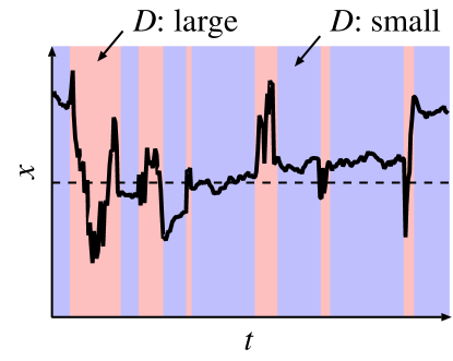
Figure 1:

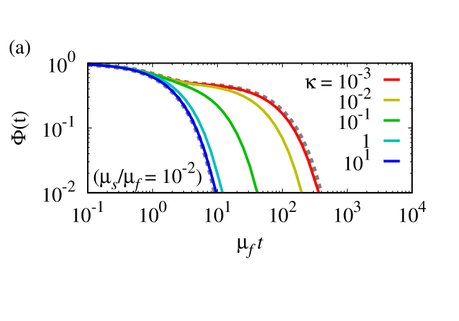
Figure 2:

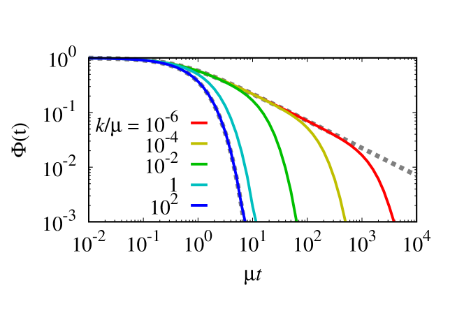
Figure 3:

References

- Chubynsky and Slater (2014) M. V. Chubynsky and G. W. Slater, Phys. Rev. Lett. 113, 098302 (2014).
- Bressloff and Newby (2014) P. C. Bressloff and J. M. Newby, Phys. Rev. E 89, 042701 (2014).
- Bressloff (2016) P. C. Bressloff, Phys. Rev. E 94, 042129 (2016).
- Massignan et al. (2014) P. Massignan, C. Manzo, J. A. Torreno-Pina, M. F. García-Parajo, M. Lewenstein, and G. J. Lapeyre, Phys. Rev. Lett. 112, 150603 (2014).
- Yamamoto et al. (2014) E. Yamamoto, T. Akimoto, Y. Hirano, M. Yasui, and K. Yasuoka, Phys. Rev. E 89, 022718 (2014).
- Manzo et al. (2015) C. Manzo, J. A. Torreno-Pina, P. Massignan, G. J. Lapeyre, M. Lewenstein, and M. F. Garcia Parajo, Phys. Rev. X 5, 011021 (2015).
- Uneyama et al. (2015) T. Uneyama, T. Miyaguchi, and T. Akimoto, Phys. Rev. E 92, 032140 (2015).
- Miyaguchi et al. (2016) T. Miyaguchi, T. Akimoto, and E. Yamamoto, Phys. Rev. E 94, 012109 (2016).
- Chechkin et al. (2017) A. V. Chechkin, F. Seno, R. Metzler, and I. M. Sokolov, Phys. Rev. X 7, 021002 (2017).
- Jain and Sebastian (2017) R. Jain and K. L. Sebastian, J. Chem. Sci. 129, 929 (2017).
- Sergé et al. (2008) A. Sergé, N. Bertaux, H. Rigneault, and D. Marguet, Nat. Methods 5, 687 (2008).
- Cherstvy and Metzler (2015) A. G. Cherstvy and R. Metzler, J. Stat. Mech. 2015, P05010 (2015).
- Cherstvy and Metzler (2016) A. G. Cherstvy and R. Metzler, Phys. Chem. Chem. Phys. 18, 23840 (2016).
- He et al. (2008) Y. He, S. Burov, R. Metzler, and E. Barkai, Phys. Rev. Lett. 101, 058101 (2008).
- Cherstvy et al. (2013) A. G. Cherstvy, A. V. Chechkin, and R. Metzler, New J. Phys. 15, 083039 (2013).
- Yang et al. (2003) H. Yang, G. Luo, P. Karnchanaphanurach, T.-M. Louie, I. Rech, S. Cova, L. Xun, and X. S. Xie, Science 302, 262 (2003).
- Hu et al. (2015) X. Hu, L. Hong, M. D. Smith, T. Neusius, X. Cheng, and J. C. Smith, Nature Phys. 12, 171 (2015).
- Doi and Edwards (1978) M. Doi and S. F. Edwards, J. Chem. Soc. Faraday Trans. 2 74, 1789 (1978).
- Doi and Edwards (1986) M. Doi and S. F. Edwards, The Theory of Polymer Dynamics (Oxford University Press, Oxford, 1986).
- Yamamoto and Onuki (1998a) R. Yamamoto and A. Onuki, Phys. Rev. Lett. 81, 4915 (1998a).
- Yamamoto and Onuki (1998b) R. Yamamoto and A. Onuki, Phys. Rev. E 58, 3515 (1998b).
- Sillescu (1999) H. Sillescu, J. Non-Cryst. Solids 243, 81 (1999).
- Evans and Morris (2008) D. J. Evans and G. P. Morris, Statistical Mechanics of Nonequilibrium Liquids, 2nd ed. (Cambridge University Press, Cambridge, 2008).
- Watanabe (1999) H. Watanabe, Prog. Polym. Sci. 24, 1253 (1999).
- Matsumiya et al. (2011) Y. Matsumiya, A. Uno, H. Watanabe, T. Inoue, and O. Urakawa, Macromolecules 44, 4355 (2011).
- van Kampen (2007) N. G. van Kampen, Stochastic Processes in Physics and Chemistry, 3rd ed. (Elsevier, Amsterdam, 2007).
- Kröger (2004) M. Kröger, Phys. Rep. 390, 453 (2004).
- Miyaguchi (2017) T. Miyaguchi, Phys. Rev. E 96, 042501 (2017).
- Baschnagel and Varnik (2005) J. Baschnagel and F. Varnik, J. Phys.: Cond. Matt. 17, R851 (2005).
- Ding and Sokolov (2006) Y. Ding and A. P. Sokolov, Macromolecules 39, 3322 (2006).
- Wong et al. (2004) I. Y. Wong, M. L. Gardel, D. R. Reichman, E. R. Weeks, M. T. Valentine, A. R. Bausch, and D. A. Weitz, Phys. Rev. Lett. 92, 178101 (2004).
- Shundo et al. (2011) A. Shundo, K. Mizuguchi, M. Miyamoto, M. Goto, and K. Tanaka, Chem. Comm. 47, 8844 (2011).
- Hori et al. (2012) K. Hori, D. P. Penaloza, A. Shundo, and K. Tanaka, Soft Matter 8, 7316 (2012).
- Florin et al. (1998) E.-L. Florin, A. Pralle, E. H. K. Stelzer, and J. K. H. Hörber, Appl. Phys. A 66, S75 (1998).
- Cherstvy et al. (2018) A. G. Cherstvy, S. Thapa, Y. Mardoukhi, A. V. Chechkin, and R. Metzler, Phys. Rev. E 98, 022134 (2018).
- Scalapino et al. (1972) D. J. Scalapino, M. Sears, and R. A. Ferrell, Phys. Rev. B 6, 3409 (1972).
- Krumhansl and Schrieffer (1975) J. A. Krumhansl and J. R. Schrieffer, Phys. Rev. B 11, 3535 (1975).
- Bishop and Krumhansl (1975) A. R. Bishop and J. A. Krumhansl, Phys. Rev. B 12, 2824 (1975).
- Godrèche and Luck (2001) C. Godrèche and J. M. Luck, J. Stat. Phys. 104, 489 (2001).
- Akimoto and Yamamoto (2016) T. Akimoto and E. Yamamoto, Phys. Rev. E 93, 062109 (2016).
- (41) T. Miyaguchi, T. Uneyama, and T. Akimoto, in preparation.
- Kleinert (2004) H. Kleinert, Path Integrals in Quantum Mechanics, Statistics, Polymer Physics, and Finantial Markets, 3rd ed. (World Scientific, Singapore, 2004).
- Swanson (1992) M. S. Swanson, Path Integrals and Quantum Processes (Academic Press, London, 1992).
- Onuki (2002) A. Onuki, Phase Transition Dynamics (Cambridge University Press, Cambridge, 2002).
- Martin et al. (1973) P. C. Martin, E. D. Siggia, and H. A. Rose, Phys. Rev. A 8, 423 (1973).
- Seifert (2012) U. Seifert, Rep. Prog. Phys. 75, 126001 (2012).
- Risken (1989) H. Risken, The Fokker-Planck Equation, 2nd ed. (Springer, Berlin, 1989).
- Tyagi and Cherayil (2017) N. Tyagi and B. J. Cherayil, J. Phys. Chem. B 121, 7204 (2017).
- Winter and Chambon (1986) H. H. Winter and F. Chambon, J. Rheol. 30, 367 (1986).
- Mason and Weitz (1995) T. G. Mason and D. A. Weitz, Phys. Rev. Lett. 74, 1250 (1995).
- Waigh (2005) T. A. Waigh, Rep. Prog. Phys. 68, 685 (2005).
- Larson (1999) R. G. Larson, The Structure and Rheology of Complex Fluids (Oxford University Press, New York, 1999).
- Fox (1977) R. F. Fox, J. Math. Phys. 18, 2331 (1977).
- Rahman (1964) A. Rahman, Phys. Rev. 136, A405 (1964).
- Schiff (1968) L. I. Schiff, Quantum Mechanics, 3rd ed. (McGraw-Hill, New York, 1968).
- Olver et al. (2010) F. W. Olver, D. W. Lozier, R. F. Boisvert, and C. W. Clark, NIST Handbook of Mathematical Functions (Cambridge University Press, New York, 2010).
- Arfken et al. (2012) G. Arfken, H. Weber, and F. E. Harris, Mathematical Methods for Physicists, 7th ed. (Academic Press, Oxford, 2012).