myclipboard

Liu, Ye, and Lee

HDSL Under Approximate Sparsity with Applications to Nonsmooth Estimation and Regularized Neural Networks

High-Dimensional Learning under Approximate Sparsity with Applications to Nonsmooth Estimation and Regularized Neural Networks

Hongcheng Liu Department of Industrial and Systems Engineering, University of Florida, Gainesville, FL 32611, liu.h@ufl.edu Yinyu Ye Department of Management Science and Engineering, Stanford University, Stanford, CA 94305, yyye@stanford.edu Hung Yi Lee Department of Industrial and Systems Engineering, University of Florida, Gainesville, FL 32611, hungyilee@ufl.edu

High-dimensional statistical learning (HDSL) has wide applications in data analysis, operations research, and decision-making. Despite the availability of multiple theoretical frameworks, most existing HDSL schemes stipulate the following two conditions: (a) the sparsity, and (b) the restricted strong convexity (RSC). This paper generalizes both conditions via the use of the folded concave penalty (FCP). More specifically, we consider an M-estimation problem where (i) the (conventional) sparsity is relaxed into the approximate sparsity and (ii) the RSC is completely absent. We show that the FCP-based regularization leads to poly-logarithmic sample complexity; the training data size is only required to be poly-logarithmic in the problem dimensionality. This finding can facilitate the analysis of two important classes of models that are currently less understood: the high-dimensional nonsmooth learning and the (deep) neural networks (NN). For both problems, we show that the poly-logarithmic sample complexity can be maintained. In particular, our results indicate that the generalizability of NNs under over-parameterization can be theoretically ensured with the aid of regularization.

Neural network, folded concave penalty, high-dimensional learning, folded concave penalty, support vector machine, nonsmooth learning, restricted strong convexity

1 Introduction

This paper is concerned with high-dimensional statistical learning (HDSL), which refers to the problems of estimating a large number of parameters with few training data. The HDSL problems are found in wide applications ranging from imaging, bioinformatics, and deep learning, etc. A standard setup of the HDSL is summarized below: We are given a sequence of $n$-many i.i.d. sample observations, denoted $Z_{i}$, $i=1,...,n$. Those observations are copies of a random vector $\mathcal{Z}$, which has unknown support $\mathcal{W}\subseteq\Re^{q}$ (for some positive integer $q$) and an unknown probability distribution. In addition to the sample observations above, we are also given a function $L(\boldsymbol{\beta},Z_{i})$, where $L:\,\Re^{p}\times\mathcal{W}\rightarrow\Re$ measures the statistical loss with respect to the data point $Z_{i}$ and the vector of fitting parameters $\boldsymbol{\beta}:=(\beta_{j})\in\Re^{p}$. Here, the positive integer $p$ is called the problem dimensionality (which is equal to the number of fitting parameters). Throughout this paper, we assume that $L$ is measurable and deterministic, the expectation $\mathbb{E}[L(\boldsymbol{\beta},\,\mathcal{Z})]$ over $\mathcal{Z}$ is well-defined for all $\boldsymbol{\beta}\in\Re^{p}$, and $\inf_{\boldsymbol{\beta}}\leavevmode\nobreak\ \mathbb{E}[L(\boldsymbol{\beta},\,\mathcal{Z})]>-\infty$. one sentenceThough no convexity assumption is imposed explicitly, many of our results are mainly useful when $L(\,\cdot\,,z)$ is convex. Given the above, it is often essential to estimate the solution to the following population-level problem in many applications:

$$\boldsymbol{\beta}^{*}\in\underset{{\boldsymbol{\beta}\in\Re^{p}}}{\arg\,\inf}\leavevmode\nobreak\ \left\{\mathbb{L}(\boldsymbol{\beta}):=\mathbb{E}[L(\boldsymbol{\beta},\,\mathcal{Z})]\right\}.$$ (1)

Here, $\boldsymbol{\beta}^{*}$ is intuitively the vector of fitting parameters which yields the smallest population-level statistical loss (a.k.a., population risk). Therefore, $\boldsymbol{\beta}^{*}$ is considered the target of estimation and referred to as the vector of “true parameters”. The HDSL problem of interest is then how to estimate (or approximate) $\boldsymbol{\beta}^{*}$, given the a-priori knowledge of the samples $\mathbf{Z}_{1}^{n}:=(Z_{1},Z_{2},...,Z_{n})$ and the formulation of $L$, when $p\geq n$. We are especially interested in the more challenging case where the sample size $n$ is much smaller than the dimensionality $p$ (i.e., $p\gg n$). In measuring the approximation quality (a.k.a., recovery quality) of an estimator $\widehat{\boldsymbol{\beta}}\in\Re^{p}$, we consider a metric of generalization error calculated as $\mathbb{L}(\widehat{\boldsymbol{\beta}})-\inf_{\boldsymbol{\beta}}\leavevmode\nobreak\ \mathbb{L}({\boldsymbol{\beta}})$. This metric is the same as the excess risk, which is discussed by Bartlett et al. (2006), Koltchinskii (2010), and Clémençon et al. (2008), among others, as an important, if not the primary, measure of generalization performance for their results.

For the HDSL problems above, most traditional schemes are not applicable, because they usually stipulate that $n>p$. For example, one popularly adopted scheme is to construct a surrogate for the population-level formulation in (1) through the sample average approximation (SAA) below:

$$\boldsymbol{\beta}^{SAA}\in\underset{\boldsymbol{\beta}}{\arg\,\inf}\,\left\{\mathcal{L}_{n}(\boldsymbol{\beta},\mathbf{Z}_{1}^{n}):=\frac{1}{n}\sum_{i=1}^{n}L(\boldsymbol{\beta},\,Z_{i})\right\},$$ (2)

where the objective function $\mathcal{L}_{n}(\boldsymbol{\beta},\mathbf{Z}_{1}^{n})$ is often also called the empirical risk function in the context of statistical and machine learning. The SAA entails desirable computational and statistical properties (many of which are discussed by Shapiro et al. 2014, and references therein) but is not designed for handling high dimensionality. Indeed, the best known upper bound on the approximation error of the SAA solution is of the order $\mathcal{O}(\sqrt{p/n})$, where $\mathcal{O}(\cdot)$ hides some quantities independent of, or poly-logarithmic in, “$\,\cdot\,$”. Consequently, the estimator of the true parameters generated by solving the SAA, as well as by most other traditional statistical learning approaches, may incur non-trivial errors when $p\gg n$.

To address high dimensionality, several statistical schemes have already been made available. (See Bühlmann and van de Geer 2011, Fan et al. 2014, for excellent reviews.) Among them, this paper follows and generalizes one of the most successful HDSL techniques introduced by Fan and Li (2001) and Zhang (2010) as in the formulation below:

$$\inf_{\boldsymbol{\beta}\in\Re^{p}} \left\{\mathcal{L}_{n,\lambda}(\boldsymbol{\beta},\,\mathbf{Z}_{1}^{n}):=\mathcal{L}_{n}(\boldsymbol{\beta},\,\mathbf{Z}_{1}^{n})+\sum_{j=1}^{p}P_{\lambda}(|\beta_{j}|)\right\},$$ (3)

where $P_{\lambda}:\,\Re_{+}\rightarrow\Re_{+}$ is a term of sparsity-inducing regularization in the form of a folded concave penalty (FCP). One mainstream special case of the existing FCPs, called the minimax concave penalty (MCP) (Zhang 2010), is of our particular consideration. The MCP is formulated as

$$P_{\lambda}(\theta)=\int_{0}^{\theta}\frac{[a\lambda-t]_{+}}{a}dt,\qquad\theta\geq 0,$$ (4)

with $[\cdot]_{+}:=\max\{0,\,\,\cdot\,\}$ and tuning parameters $a,\,\lambda>0$. (Hereafter, we use the term “FCP” to refer to the MCP exclusively.) Eq. (3) is nonconvex, to which the local and/or global solutions have been shown to entail desirable statistical performance (Loh and Wainwright 2015, Wang et al. 2013, 2014, Zhang and Zhang 2012, Loh 2017). to understand the roles copyTo understand the roles of the tuning parameters $a$ and $\lambda$ to the FCP, we may observe that its first derivative, $P_{\lambda}^{\prime}(\theta)$, is a non-increasing function with $P_{\lambda}^{\prime}(0)=\lambda$ and $P_{\lambda}^{\prime}(\theta)=0$ for all $\theta\geq a\lambda$. This means that $\lambda$ determines how intense the penalty is to induce a fitting parameter that is almost zero to be exactly zero. The intensity of this penalty becomes smaller as the magnitude of the corresponding fitting parameter increases. Once the absolute value of that parameter is beyond the threshold $a\lambda$, the penalty becomes a constant and thus (locally) ineffective. Furthermore, we also observe that $P_{\lambda}^{\prime\prime}(\theta)=-\frac{1}{a}$ for all $\theta\in(0,\,a\lambda)$ and $P_{\lambda}^{\prime\prime}(\theta)=0$ for all $\theta>a\lambda$. Therefore, $a$ determines the curvature of the FCP near the origin.

Alternative sparsity-inducing penalties senAlternative sparsity-inducing penalties, such as the smoothly clipped absolute deviation (SCAD) introduced by Fan and Li (2001), the least absolute shrinkage and selection operator (Lasso) proposed by Tibshirani (2011), and the bridge penalty (a.k.a., the $\ell_{\mathbf{q}}$ penalty with $0<\mathbf{q}<1$) as discussed by Frank and Friedman (1993), have all been shown to be very effective in HDSL by many results due to Fan and Li (2001), Bickel et al. (2009), Fan and Lv (2011), Fan et al. (2014), Loh and Wainwright (2015), Raskutti et al. (2011), Negahban et al. (2012), Wang et al. (2013, 2014), Zhang and Zhang (2012), Zou (2006), Zou and Li (2008), Liu et al. (2017, 2018) and Loh (2017), to name only a few. Many of those results provide oracle inequalities, which “relates the performance of a real estimator with that of an ideal estimator” (Candes 2006). Ndiaye et al. (2017), Ghaoui et al. (2010), Fan and Li (2001), Chen et al. (2010), and Liu et al. (2017) have presented thresholding rules and bounds on the number of nonzero dimensions for a high-dimensional linear regression problem with different penalty functions.

Despite the availability of several analytical frameworks for HDSL in the current literature, most existing HDSL theories require the two assumptions below, which are sometimes overly critical, to guarantee any generalization performance:

• The satisfaction of the (conventional) sparsity condition, written as $\|\boldsymbol{\beta}^{*}\|_{0}\ll p$, where $\|\cdot\|_{0}$ denotes the number of nonzero entries of a vector.

• The satisfaction of regularity conditions on the eigenvalues of the Hessian matrix of $L(\,\cdot\,,\mathcal{Z})$ in the form of the restricted strong convexity (RSC) (Negahban et al. 2012), the restricted isotropic property (RIP) (Candes and Tao 2007), or the restricted eigenvalue (RE) condition (Bickel et al. 2009).

The sparsity assumption essentially means that few dimensions “matter” despite that the total number of dimensions is very high. Meanwhile, the RSC, RIP, and RE can all be interpretable as the stipulation that $\mathcal{L}(\,\cdot\,,\mathbf{Z}_{1}^{n})$ is strongly convex everywhere in some subset of $\Re^{p}$. The RSC is implied by the RE and RIP for some choices of parameters (Negahban et al. 2012, van de Geer et al. 2009). Except for some special cases of the generalized linear models (as discussed by, e.g., Bickel et al. 2009), when both (A) and (B) above are violated, little is known about the performance of (3) or that of most other HDSL schemes in terms of their generalization performance in general. Negahban et al. (2012) has considered HDSL under weak sparsity, but the RSC is still assumed for establishing the generalization error bounds.

In contrast to the literature, this paper is concerned with the effectiveness of (3) in addressing the HDSL problems when the RSC is completely absent and the traditional sparsity is relaxed into the approximate sparsity (A-sparsity) as below. $\mathbb{L}(\boldsymbol{\beta}^{*}_{{\varepsilon_{A}}})-\inf_{\boldsymbol{\beta}}\mathbb{L}(\boldsymbol{\beta})\leq{\varepsilon_{A}}$ and $s:=\|\boldsymbol{\beta}^{*}_{\varepsilon_{A}}\|_{0}\ll p$ for some $\varepsilon_{A}\geq 0$, $\boldsymbol{\beta}_{\varepsilon_{A}}^{*}:\,\|\boldsymbol{\beta}_{\varepsilon_{A}}^{*}\|_{\infty}\leq R$, and $R\geq 1$. Intuition Assumption A-sparsity CopyIntuitively, Assumption 1 means that, although $\boldsymbol{\beta}^{*}$ can be dense, replacing most of the nonzero entries of $\boldsymbol{\beta}^{*}$ by zero does not cause the population risk to increase too much. It is evident that, if $\varepsilon_{A}=0$, Assumption 1 is reduced to the (traditional) sparsity.

In certain applications of HDSL (e.g., the deep neural networks to be discussed subsequently), it is more convenient to consider a (slight) generalization to Assumption 1 in the following.

$\mathbb{L}(\boldsymbol{\beta}^{*}_{{\varepsilon_{A}}})-L_{g}^{*}\leq{\varepsilon_{A}}$ and $s:=\|\boldsymbol{\beta}^{*}_{\varepsilon_{A}}\|_{0}\ll p$ for some $\varepsilon_{A}\geq 0$, $\boldsymbol{\beta}_{\varepsilon_{A}}^{*}:\,\|\boldsymbol{\beta}_{\varepsilon_{A}}^{*}\|_{\infty}\leq R$, $L_{g}^{*}\leq\inf_{\boldsymbol{\beta}}\leavevmode\nobreak\ \mathbb{L}(\boldsymbol{\beta})$, and $R\geq 1$. Apparently, Assumption 1 is more general than Assumption 1, and the two are equivalent when $L_{g}^{*}=\inf_{\boldsymbol{\beta}}\leavevmode\nobreak\ \mathbb{L}({\boldsymbol{\beta}})$. Hereafter, both Assumptions 1 and 1 are referred to as A-sparsity when there is no ambiguity. Without loss of generality, we let $s>1$ throughout this paper.

to copy 2The assumption of $\|\boldsymbol{\beta}_{\varepsilon_{A}}^{*}\|_{\infty}\leq R$ is non-critical. It is comparable to, if not less restrictive than, some common assumptions in the literature. For example, in addressing HDSL under (the conventional) sparsity, Loh (2017) and Loh and Wainwright (2015) both assume the estimator and the vector of true parameters to be contained within a convex and bounded set of $\{\boldsymbol{\beta}:\,|\boldsymbol{\beta}|\leq R_{\ell_{1}}\}$ for some $R_{\ell_{1}}>0$. Verifiably, under their assumptions, $\|\boldsymbol{\beta}_{\varepsilon_{A}}^{*}\|_{\infty}\leq R$ holds with some $R\leq R_{\ell_{1}}$. Furthermore, we later show that our generalization error bounds depend only logarithmically on $R$. Thus, it is flexible to pick the value of $R$ in practice; we only need to have a coarse estimation of an upper bound on $\|\boldsymbol{\beta}_{\varepsilon_{A}}^{*}\|_{\infty}$. Even if $R$ overestimates $\|\boldsymbol{\beta}_{\varepsilon_{A}}^{*}\|_{\infty}$ too much, the performance of the proposed scheme would probably not be impacted significantly.

We believe that the flexibility of A-sparsity and the relaxation of the RSC can allow the HDSL theories to cover a more comprehensive class of applications. Indeed, as we are to articulate later, our results on HDSL under A-sparsity can facilitate the comprehension of two important classes of problems whose theoretical underpinnings are currently lacking from the literature: (i) A high-dimensional nonsmooth learning problem (nonsmooth HDSL), that is, an HDSL problem with a nonsmooth empirical risk function, and (ii) a (deep and over-parameterized) neural network (NN) model.

Weak sparsity discussion 1 contentMore general forms of sparsity, such as the weak sparsity assumption (Negahban et al. 2012), have been discussed previously. However, the only existing discussions on simultaneously relaxing both the sparsity and the RSC assumptions are due to Liu et al. (2018), to our knowledge. Their results imply that the excess risk of an estimator $\widehat{\boldsymbol{\beta}}\in\Re^{p}$ generated as a certain stationary point to the formulation (3) can be bounded by ${\mathcal{O}}\left(\frac{\sqrt{\ln p}}{n^{1/4}}\cdot\left(1+\sqrt{\varepsilon_{A}}\right)+\varepsilon_{A}\right)$. This bound is reduced to ${\mathcal{O}}\left(\frac{\sqrt{\ln p}}{n^{1/4}}\right)$ when $\varepsilon_{A}=0$. In contrast, our findings in the current paper can strengthen the previous results. More specifically, we relax the subgaussian assumption stipulated by Liu et al. (2018) and impose the weaker, subexponential, condition instead. In addition, the assumption of twice-differentiability made by Liu et al. (2018) is also weakened. In the more general settings, we further show that sharper error bounds can be achieved at a stationary point that (a) satisfies a set of significant subspace second-order necessary conditions (S³ONC) to be formalized subsequently, and (b) has an objective function value no worse than that of the solution to the Lasso problem, formulated below:

$$\min_{\boldsymbol{\beta}\in\Re^{p}}\left\{\mathcal{L}_{n}(\boldsymbol{\beta},\,\mathbf{Z}_{1}^{n})+\sum_{j=1}^{p}\lambda\cdot|\beta_{j}|\right\}.$$ (5)

We are to discuss some S³ONC-guaranteeing algorithms to meet the first requirement soon afterwards. To meet the second requirement, we may always initialize the S³ONC-guaranteeing algorithm with a solution to (5), which is often polynomial-time solvable if $\mathcal{L}_{n}(\,\cdot\,,\mathbf{Z}_{1}^{n})$ is convex.

Our new bounds on those S³ONC solutions are summarized below. First, in the case where $\varepsilon_{A}=0$, we can bound the excess risk by ${\mathcal{O}}\left(\frac{{\ln p}}{n^{2/3}}+\frac{\sqrt{\ln p}}{n^{1/3}}\right)$, which is better than the aforementioned result by Liu et al. (2018) in terms of the dependance on $n$. Second, when $\varepsilon_{A}$ is nonzero, the excess risk is then bounded by

$$\mathbb{L}(\widehat{\boldsymbol{\beta}})-\inf_{\boldsymbol{\beta}}\leavevmode\nobreak\ \mathbb{L}(\boldsymbol{\beta})\leq{\mathcal{O}}\left(\frac{\ln p}{n^{2/3}}+{\frac{\sqrt{\ln p}}{n^{1/3}}}+\sqrt{\frac{\varepsilon_{A}}{n^{1/3}}}+\varepsilon_{A}\right).$$ (6)

Third, if we further relax the requirement above and consider an arbitrary S³ONC solution, then the excess risk becomes

$$\mathbb{L}(\widehat{\boldsymbol{\beta}})-\inf_{\boldsymbol{\beta}}\leavevmode\nobreak\ \mathbb{L}(\boldsymbol{\beta})\leq{\mathcal{O}}\left(\frac{{\ln p}}{n^{2/3}}+\sqrt{\frac{{\ln p}}{n}}+\frac{1}{n^{1/3}}+\sqrt{\frac{\Gamma+\varepsilon_{A}}{n^{1/3}}}+\Gamma+\varepsilon_{A}\right),$$ (7)

where $\Gamma\geq 0$ is (an underestimation of) the suboptimality gap that this S³ONC solution incurs in minimizing $\mathcal{L}_{n,\lambda}(\,\cdot\,,\mathbf{Z}_{1}^{n})$ (as defined in (3)).

Admittedly, our excess risk bounds are less appealing than the generalizability results made available in some important previous works by Loh (2017), Raskutti et al. (2011), and Negahban et al. (2012), etc., under the assumption of the RSC. In contrast, we argue that our results are established under a more general set of conditions and can complement the existing results in the HDSL problems beyond the RSC. para in GammaIt is also worth noting that (7) is in the parameterization of $\Gamma$, which can only be explicitly controlled when $\mathcal{L}_{n}(\,\cdot,\,\mathbf{Z}_{1}^{n})$ is convex in general. Nonetheless, we argue that, in some interesting special cases, one may still control $\Gamma$ despite the absence of convexity. One of such examples is presented in this paper as we discuss the theoretical applications of HDSL under A-sparsity to the NNs in Sections 6 and 9.

The S³ONC is a necessary condition for local minimality. Compared to the second-order KKT conditions, the S³ONC is weaker and potentially easier computable. To generate a solution that satisfies the S³ONC admits pseudo-polynomial-time algorithms, such as the variants of Newton’s method proposed by Haeser et al. (2017), Bian et al. (2015), Ye (1992, 1998) and Nesterov and Polyak (2006). All those algorithms provably ensure a $\gamma_{opt}$-approximation (with a user-specified error tolerance $\gamma_{opt}>0$) to the second-order KKT conditions at the best-known iteration complexity of the rate ${\mathcal{O}}(1/\gamma_{opt}^{3})$. The second-order KKT conditions then imply the S³ONC. To add to the current solution schemes, we derive a new gradient-based method that provably guarantees the S³ONC. In contrast to the literature, the iteration complexity of this new algorithm is ${\mathcal{O}}(1/\gamma_{opt}^{2})$, which improves upon the existing alternatives. Due to the gradient-based nature of the proposed algorithm, it does not access the Hessian matrix or its inverse. Therefore, we think that this gradient-based algorithm may be of some independent interest.

1.1 Some theoretical applications

As mentioned, our results on HDSL under A-sparsity can be employed in the analysis of two important classes of statistical and machine learning models: (a) nonsmooth HDSL, and (b) deep NNs. Some additional details are provided below.

1.1.1 Nonsmooth HDSL.

Although several special cases of HDSL with nonsmoothness, such as high-dimensional least absolute regression, high-dimensional quantile regression, and high-dimensional support vector machine (SVM) have been discussed by Wang (2013), Belloni and Chernozhukov (2011), Zhang et al. (2016b, c) and Peng et al. (2016), there exist few theories that apply to scenarios without an everywhere differentiable loss function in general, especially when non-differentiability may occur at, or in a near neighborhood of, the vector of true parameters.

In contrast, our theories on HDSL under A-sparsity can be utilized to understand the generalization performance of a flexible set of nonsmooth HDSL problems. Indeed, their nonsmooth statistical loss functions can be approximated by another formulation that preserves the continuous differentiability, and the resulting approximation error can then be handled through the notion of A-sparsity. Analyzing this approximation leads to the following bound on the excess risk at an S³ONC solution when the vector of true parameters is A-sparse in the sense of Definition 1:

$${\mathcal{O}}\left(\frac{{\ln p}}{n^{3/4}}+\frac{\sqrt{\ln p}}{n^{1/4}}+\sqrt{\frac{\varepsilon_{A}}{n^{1/4}}}+\varepsilon_{A}\right).$$ (8)

In particular, under the conventional sparsity assumption (that is, when $\varepsilon_{A}=0$), the rate above becomes ${\mathcal{O}}\left(\frac{{\ln p}}{n^{3/4}}+\frac{\sqrt{\ln p}}{n^{1/4}}\right)$. To our knowledge, this is perhaps the first generic theory for the high-dimensional M-estimation problems in which the empirical risk function may not be everywhere differentiable.

1.1.2 Regularized neural network.

The NNs have been frequently discussed and widely applied in recent literature (Schmidhuber 2015, LeCun et al. 2015, Yarotsky 2017). Despite the frequent and exciting advancements in the NN-related algorithms, models, and applications, the development of their theoretical underpinnings is seemingly lagging behind. DeVore et al. (1989), Yarotsky (2017), Mhaskar and Poggio (2016), and Mhaskar (1996), etc., have explicated the expressive power of the NNs in the approximation of different types of functions. As for the generalizability of NNs, one of the focuses of this paper, effective theoretical frameworks have been discussed by Cao and Gu (2019), Li and Liang (2018), Brutzkus et al. (2017), Allen-Zhu et al. (2019), Wang et al. (2019b), Daniely (2017), Neyshabur et al. (2015), Bartlett et al. (2017), Hardt et al. (2015), Zhang et al. (2016a), Li et al. (2018), Jakubovitz et al. (2019), among others. However, for the vast majority of the existing results on the deep NNs, the generalization error bounds grow polynomially in the dimensionality (which is equal to the number of fitting parameters and is also called the network size) and sometimes even increase exponentially in the depth of the network. Such a high sensitivity to dimensionality and depth is inconsistent with the empirical performance of the NNs in many practical applications, where over-parameterization and deep architectures are common and often preferred by practitioners.

In contrast, we analyze the NNs through the lens of HDSL under A-sparsity and consider an FCP-regularized NN training formulation as a special case of (3) in binary classification. Our results indicate that the NN’s generalization errors at local solutions can be both poly-logarithmic in the number of fitting parameters and polynomial in the network depth. Thus, we think that the results herein can facilitate understanding the powerful performance of the NNs in practice, especially for the over-parameterized and deep models. Barron and Klusowski (2018) have shown the existence of fitting parameters for an NN with ramp activation functions to achieve the poly-logarithmic sample complexity. Compared with Barron and Klusowski (2018), our analysis may present better flexibility in the choice of activation functions and provide more insights towards the computability of the desired fitting parameters in training a deep NN to ensure the proven error bounds.

More specifically, we show that the generalization error incurred by an S³ONC solution to the FCP-regularized training formulation of an NN is bounded by

$${\mathcal{O}}\left(\underbrace{\frac{{s_{A}}\cdot\mathcal{D}\cdot\ln p}{n^{2/3}}+\sqrt{\frac{{s_{A}}\cdot\mathcal{D}\cdot\ln p}{n}}+\frac{1}{n^{1/3}}}_{\text{$\mathcal{O}\left(n^{-1/3}+n^{-1/2}\mathcal{D}\cdot\ln p\right)$}}+\underbrace{\Gamma}_{\text{Suboptimality gap}}+\underbrace{\Omega({s_{A}})}_{\text{Representability gap}}+\underbrace{\sqrt{\frac{\Gamma+\Omega({s_{A}})}{n^{1/3}}}}_{\text{Interaction term}}\right),$$ (9)

for any fixed ${s_{A}}:\,1\leq{s_{A}}\leq p$, with overwhelming probability. Here, $\mathcal{D}$ is the number of NN layers, $\Gamma\geq 0$ is the suboptimality gap incurred by the S³ONC solution of consideration, and $\Omega({p^{\prime}})$, for any ${p^{\prime}}:\,1\leq{p^{\prime}}\leq p$, is the architecture-dependent representability gap (a.k.a., the model misspecification error or the expressive power) of an NN with ${p^{\prime}}$-many nonzero fitting parameters. By (9) above, the generalization error of an NN consists of four terms: (i) a generalization error term of the order $\mathcal{O}\left(n^{-1/3}+n^{-1/2}\mathcal{D}\ln p\right)$; (ii) the suboptimality gap; (iii) a term that measures the NN’s representability; and (iv) a term that is dependent on suboptimality gap, sample size, and representability, simultaneously. It is worth noting that (9) is obtained with little restriction on the NN architecture and the data generation process. Combining (9) with the existing results on the representability analysis of NNs, we further derive more explicit generalization error bounds. For example, we show that the error yielded by an NN with smooth activation functions can be bounded by ${\mathcal{O}}\left(\frac{\mathcal{D}\cdot\ln p}{n^{1/3}}+\sqrt{{\frac{\Gamma}{n^{1/3}}}}+\Gamma\right)$, when we assume that data from different categories are separable by a polynomial function (as well as a couple of other conditions on the NN architecture).

Error bound in dependsThe error bound in (9) depends on $\Gamma$, the suboptimality gap. To explicitly bound its value is challenging in general because of the nonconvexity of an NN’s training formulation. Nonetheless, we show that some pseudo-polynomial-time computable solutions generated with the aid of an efficient initialization provably ensure the explicit control of $\Gamma$ in the same settings considered by Cao and Gu (2020). In such a case, the generalization error is further explicated into

$$\mathcal{O}\left(\frac{\mathcal{D}}{n^{1/3}}\cdot\ln p\right),$$ (10)

which becomes independent of $\Gamma$. In achieving this result, our settings seem more general than Wang et al. (2019a), and our rates on both $\mathcal{D}$ and $p$ are perhaps more appealing than most of the existing results. In particular, Wang et al. (2019a) focus on ReLU-NNs (that is, the NNs where the activation functions are ReLU, as discussed by Glorot et al. 2011) with one hidden layer, but our approach can handle deep NNs under more general hyper-parameters. For deep and wide NNs, Cao and Gu (2020) have established generalization error bounds, which, however, increase exponentially in the number of layers in the same settings of our discussion. In contrast, our bound is both poly-logarithmic in dimensionality and polynomial in the number of layers. The computational complexity of training an NN with the claimed error bound is in pseudo-polynomial time.

In obtaining our results, we do not artificially impose any condition on sparsity or alike. As we articulate in Section 6.2, our findings are based on the observation that the A-sparsity (as in Assumption 1) is an intrinsic property implied by the NN’s expressive power.

1.2 Summary of results

Table 1 summarizes the sample complexity results proven in this paper. In contrast to the literature, we claim that our results could lead to the following contributions:

• We provide the first HDSL theory for problems where the three conditions—the twice-differentiability, the RSC or alike, and the sparsity—are simultaneously relaxed. In the more general settings, we show that HDSL is still possible even if the sample size is only poly-logarithmic in the dimensionality. In Table 1, the results are presented in the rows for “HDSL under A-sparsity”.

• We have derived a pseudo-polynomial-time gradient-based method to compute an S³ONC solution. Even though the S³ONC is a set of second-order necessary conditions, the proposed algorithm does not need to access the Hessian matrix. Furthermore, the iteration complexity of the proposed method is provably $\mathcal{O}(\frac{1}{\gamma_{opt}^{2}})$ in achieving a $\gamma_{opt}$-approximation to the S³ONC, which is sharper than the more generic algorithms such as the variations of Newton’s method.

• As theoretical applications CopyAs theoretical applications of our error bounds for HDSL under A-sparsity, we derive generalizability results for nonsmooth HDSL problems and deep NNs. More specifically, for a flexible class of high-dimensional nonsmooth M-estimation problems, we prove perhaps the first poly-logarithmic sample complexity bound without the RSC assumption. The corresponding result is summarized in Table 1 in the rows for “Nonsmooth HDSL under A-sparsity”. As for the NNs, our sample requirement is only poly-logarithmic in the network size and polynomial in the number of layers, providing theoretical underpinnings for the generalizability of an NN under over-parameterization. These results are summarized in the rows for “Neural Network” of Table 1.

Table 1: Summary of sample complexities. $\varepsilon_{A}$ is the parameter for A-sparsity as in Assumption 1. $p$ and $n$ are the sample size and the dimensionality, respectively. “ReLU-NN” stands for an NN with ReLU activation.

HDSL under A-sparsity
S3ONC initialized with Lasso	$\frac{\ln p}{n^{2/3}}+{\frac{\sqrt{\ln p}}{n^{1/3}}}+\sqrt{\frac{\varepsilon_{A}}{n^{1/3}}}+\varepsilon_{A}$
S3ONC with suboptimality gap $\Gamma$	$\frac{{\ln p}}{n^{2/3}}+\sqrt{\frac{{\ln p}}{n}}+\frac{1}{n^{1/3}}+\sqrt{\frac{\Gamma+\varepsilon_{A}}{n^{1/3}}}+\Gamma+\varepsilon_{A}$
Nonsmooth HDSL under A-sparsity
S3ONC initialized with Lasso	$\frac{{\ln p}}{n^{3/4}}+\frac{\sqrt{\ln p}}{n^{1/4}}+\sqrt{\frac{\varepsilon_{A}}{n^{1/4}}}+\varepsilon_{A}$
Neural network (with $\mathcal{D}$-many layers and $p$-many fitting parameters)
S3ONC to a general NN with suboptimality gap $\Gamma$ and any $s_{A}:\,1\leq s_{A}\leq p$	${\frac{{s_{A}}\cdot\mathcal{D}\cdot\ln p}{n^{2/3}}+\sqrt{\frac{{s_{A}}\cdot\mathcal{D}\cdot\ln p}{n}}+\frac{1}{n^{1/3}}}+{\Omega({s_{A}})}+{\Gamma}+{\sqrt{\frac{\Gamma+\Omega({s_{A}})}{n^{1/3}}}}$
S3ONC to an NN for a flexible choice of activation functions with suboptimality gap $\Gamma$, when the target function is polynomial	$\frac{\mathcal{D}}{n^{1/3}}\cdot\ln p+\sqrt{{\frac{\Gamma}{n^{1/3}}}}+\Gamma$
A pseudo-polynomial-time computable solution in training a ReLU-NN in the same settings by Cao and Gu (2020)	$\frac{\mathcal{D}}{n^{1/3}}\cdot\ln p$

1.3 Organization of the paper

The rest of the paper is organized as below: Section 2 summarizes the settings and assumptions. Section 3 introduces the S³ONC. Section 4 states our main results concerning HDSL under A-sparsity. A pseudo-polynomial-time solution scheme that guarantees the S³ONC is discussed in Section 5. Section 6 discusses the theoretical applications to nonsmooth HDSL and the regularized (deep) NNs. Some numerical experiments are presented in Section 7. Sections 9 and 10 of the electronic companion, respectively, present some additional theoretical results on the NN and supplementary numerical results on both the SVM and the NN. Section 8 concludes the paper.

Our notations are summarized below. We use $p$ and $n$ to represent the numbers of dimensions (fitting parameters) and the sample size. We let $\|\,\cdot\,\|_{\mathbf{p}}$ ($1\leq\mathbf{p}\leq\infty$) be the $\mathbf{p}$-norm, except that $1$- and $2$-norms are denoted by $|\,\cdot\,|$ and $\|\,\cdot\,\|$, respectively. When there is no ambiguity, we also denote by $|\,\cdot\,|$ the cardinality of a set, if the argument is a finite set. Let $\|\cdot\|_{F}$ of a matrix be its Frobenius norm and let $\|\cdot\|_{0}$ of a vector be the number of its nonzero entries. For a random vector $\mathbf{v}=(v_{j})\in\Re^{p}$, we denote that $\|\mathbf{v}\|_{\infty}\leq R$ if $\mathbb{P}[|v_{j}|\leq R,\,\forall j=1,...,p]=1$. For a random variable $X$, its subexponential and subgaussian norms are denoted by $\|X\|_{\psi_{1}}$ and $\|X\|_{\psi_{2}}$, respectively. defi of norm Copy$\|\mathbf{A}\|_{1,2}:=\max_{\mathbf{x}\in\Re^{m_{1}},\,\mathbf{u}\in\Re^{m_{2}}}\{\mathbf{u}^{\top}\mathbf{A}\mathbf{x}:\,\|\mathbf{x}\|_{1}=1,\,\|\mathbf{u}\|_{2}=1\}$ for integers $m_{1},\,m_{2}$ and a matrix $\mathbf{A}\in\Re^{m_{2}\times m_{1}}$. For a function $f$, denote by $\nabla f$ its gradient, whenever it exists. For a vector $\boldsymbol{\beta}=(\beta_{j})\in\Re^{p}$ and a set $S\subset\{1,...,p\}$, let $\boldsymbol{\beta}_{S}=(\beta_{j}:\,j\in S)$ be a sub-vector of $\boldsymbol{\beta}$. For any vector $\mathbf{v}=(v_{j})$, the notation $diag(\mathbf{v})$ represents the diagonal matrix whose $j$th diagonal entry is $v_{j}$. We denote by $vec(M_{1},M_{2},...,M_{m})$ the vector that collects all the entries of the matrices $M_{1}$, $M_{2},$ …, $M_{m}$. The vector $e_{j}$ is the $j$th standard basis. $\lceil x\rceil$ (or $\lfloor x\rfloor$) for any $x\geq 0$ is the smallest (or largest) integer that is greater (or smaller, respectively) than or equal to $x$. Finally, we denote by $O(\cdot)$’s and $\mathcal{O}(\cdot)$’s, respectively, the complexity rates that hide (potentially different) universal constants and quantities at most logarithmically dependent on “$\cdot$”.

2 Settings and assumptions

In this section, we summarize our assumptions in addition to the aforementioned settings. We assume that the gradient $\nabla L(\boldsymbol{\beta},z):=(\frac{\partial L(\boldsymbol{\beta},z)}{\partial\beta_{j}}:\,j=1,...,p)$ of $L(\boldsymbol{\beta},z)$ w.r.t. $\boldsymbol{\beta}$ is well-defined for all $\boldsymbol{\beta}\in\Re^{p}$ and almost every $z\in\mathcal{W}$. Furthermore, we also suppose that $\frac{\partial L(\boldsymbol{\beta},z)}{\partial\beta_{j}}$ is Lipschitz continuous for all $\boldsymbol{\beta}\in\Re^{p}$; that is, there exists a scalar $U_{L}>0$ such that

$$\left|\left[\frac{\partial L(\boldsymbol{\beta},z)}{\partial\beta_{j}}\right]_{\boldsymbol{\beta}=\widetilde{\boldsymbol{\beta}}+\delta\cdot e_{j}}-\left[\frac{\partial L(\boldsymbol{\beta},z)}{\partial\beta_{j}}\right]_{\boldsymbol{\beta}=\widetilde{\boldsymbol{\beta}}}\right|\leq U_{L}\cdot|\delta|,$$ (11)

for almost every $z\in\mathcal{W}$ and for all $\widetilde{\boldsymbol{\beta}}\in\Re^{p}$, $\delta\in\Re$, $j=1,...,p$. These regularities are to be relaxed when we later discuss the nonsmooth HDSL problems and the ReLU-NNs. Apart from the above, two additional assumptions are imposed.

For all $\boldsymbol{\beta}\in\Re^{p}:\,\|\boldsymbol{\beta}\|_{\infty}\leq R$ and $i=1,...,n$, it holds that $\mathbb{E}[L(\boldsymbol{\beta},\,Z_{i})]$ is finite-valued and $L(\boldsymbol{\beta},\,Z_{i})-\mathbb{E}[L(\boldsymbol{\beta},\,Z_{i})]$ follows a subexponential distribution; that is, $\|L(\boldsymbol{\beta},\,Z_{i})-\mathbb{E}[L(\boldsymbol{\beta},\,Z_{i})]\|_{\psi_{1}}\leq\sigma,$ for some $\sigma\geq 1$.

Remark 2.1

As an implication of Assumption 2, for all $\boldsymbol{\beta}\in\Re^{p}:\,\|\boldsymbol{\beta}\|_{\infty}\leq R$, (combined with the assumption that $Z_{i}$, $i=1,...,n$, are i.i.d.) a well-known Bernstein-like inequality holds as below:

$$\mathbb{P}\left(\left|\sum_{i=1}^{n}a_{i}\left\{L(\boldsymbol{\beta},\,Z_{i})-\mathbb{E}[L(\boldsymbol{\beta},\,Z_{i})]\right\}\right|>\sigma\cdot\left(\|\mathbf{a}\|\sqrt{t}+\|\mathbf{a}\|_{\infty}t\right)\right)\leq 2\exp\left(-ct\right),\quad\forall t\geq 0,\,\mathbf{a}=(a_{i})\in\Re^{n},$$ (12)

for some absolute constant $c\in(0,\,0.5]$. Interested readers are referred to Vershynin (2012) for more detailed discussions on the subexponential distributions.

For some measurable and deterministic function $\mathcal{C}:\,\mathcal{W}\rightarrow\Re_{+}$, the random variable $\mathcal{C}(Z_{i})$ satisfies that $\left\|\mathcal{C}(Z_{i})-\mathbb{E}\left[\mathcal{C}(Z_{i})\right]\right\|_{\psi_{1}}\leq\sigma_{L},$ for all $i=1,...,n$, for some $\sigma_{L}\geq 1$. Furthermore, $|L(\boldsymbol{\beta}_{1},\,z)-L(\boldsymbol{\beta}_{2},\,z)|\leq\mathcal{C}(z)\|\boldsymbol{\beta}_{1}-\boldsymbol{\beta}_{2}\|,$ for all $\boldsymbol{\beta}_{1},\,\boldsymbol{\beta}_{2}\in\Re^{p}\cap\{\boldsymbol{\beta}:\,\|\boldsymbol{\beta}\|_{\infty}\leq R\}$ and almost every $z\in\mathcal{W}$.

Hereafter, we let $\mathbb{E}[\mathcal{C}(Z_{i})]\leq\mathcal{C}_{\mu}$ for all $i=1,...,n$ for some $\mathcal{C}_{\mu}\geq 1$.

Remark 2.2

Assumptions 2 and 2 are general enough to cover a wide spectrum of M-estimation problems. More specifically, Assumption 2 requires that the underlying distribution is sub-exponential, and Assumption 2 essentially imposes the Lipschitz(-like) continuity on $\mathcal{L}_{n}(\,\cdot\,,\mathbf{Z}_{1}^{n})$. Examples of sub-exponential distributions include uniform, Gaussian, exponential, and $\chi^{2}$ distributions, as well as any distribution that has a bounded support set. to copy remark 2As for the Lipschitz continuity, it is a condition satisfied by many statistical learning problems, such as linear regression, Huber regression, SVM, and NNs. We are to show that the generalization error bounds only grow logarithmically in the Lipschitz constant. The combination of our Assumptions is non-trivially weaker than the settings in Liu et al. (2017, 2018). It is also worth mentioning that the stipulations of $\sigma\geq 1$, $\mathcal{C}_{\mu}\geq 1$, and $\sigma_{L}\geq 1$ can be easily relaxed and are needed only for notational simplicity in presenting our results.

3 Significant subspace second-order necessary conditions

Because the FCP is nonconvex, so is Eq. (3). Thus, computing the global solution to (3) is intractable. Nonetheless, our theories concern only local stationary points. We show that these local solutions are good enough to ensure the promised statistical performance.

In particular, we consider the stationary points that are characterized by the satisfaction of the significant subspace second-order necessary conditions (S³ONC), which are closely similar to the necessary conditions discussed by Chen et al. (2010) for linear regression with bridge regularization and by Liu et al. (2017, 2018) under the assumption that the empirical risk function is everywhere twice differentiable. This paper generalizes the characterizations of the S³ONC to scenarios where the twice-differentiability may not hold everywhere.

Definition 3.1

Given $\mathbf{Z}_{1}^{n}\in\mathcal{W}^{n}$, a vector $\widehat{\boldsymbol{\beta}}\in\Re^{p}$ is said to satisfy the S³ONC (denoted by S³ONC$(\mathbf{Z}_{1}^{n})$) of Problem (3) if both of the following sets of conditions are satisfied:

1. the first-order KKT copyThe first-order KKT conditions are met at $\widehat{\boldsymbol{\beta}}:=(\widehat{\beta}_{j})$; that is, there exists $\varkappa_{j}\in\partial(|\widehat{\beta}_{j}|)$, for all $j=1,...,p$, such that

   $$\nabla\mathcal{L}_{n}(\widehat{\boldsymbol{\beta}},\,\mathbf{Z}_{1}^{n})+(P^{\prime}_{\lambda}(|\widehat{\beta}_{j}|)\cdot\varkappa_{j}:\,j=1,...p)=\mathbf{0},$$ (13)

   where $\nabla\mathcal{L}_{n}(\widehat{\boldsymbol{\beta}},\,\mathbf{Z}_{1}^{n})$ is the gradient of $\mathcal{L}_{n}(\,\cdot,\,\mathbf{Z}_{1}^{n})$ as defined in (2), $\partial(|\widehat{\beta}_{j}|)$ is the subdifferential of $|\,\cdot\,|$ at $\widehat{\beta}_{j}$, and $P^{\prime}_{\lambda}(\,\cdot\,)$ is the first derivative of $P_{\lambda}(\,\cdot\,)$.

2. The following inequality holds at $\widehat{\boldsymbol{\beta}}$: for all $j=1,...,p$, if $|\widehat{\beta}_{j}|\in(0,\,a\lambda)$, then

   $$U_{L}+P^{\prime\prime}_{\lambda}(|\widehat{\beta}_{j}|)\geq 0.$$ (14)

   where $P^{\prime\prime}_{\lambda}$ is the second derivative of $P_{\lambda}(\,\cdot\,)$, the quantity $U_{L}$ is defined as in (11), and $a$ and $\lambda$ are (hyper-)parameters of the FCP as in (4).

It is worth noting that the S³ONC is verifiably implied by the conventional second-order KKT conditions when they are well-defined. We show in Section 5 that an S³ONC solution (i.e., a solution that satisfies the S³ONC) can be computed by the proposed gradient-based method at pseudo-polynomial-time complexity.

4 Statistical performance bounds

This section presents the promised sample complexity results for a generic HDSL problem under A-sparsity. More specifically, Proposition 1 shows the most general result of this paper. In that proposition, a hyper-parameter $\varrho$ is left to be determined in different special cases. One of those cases is then presented in Theorem 4.9. For convenience, we adopt a short-hand notation as follows: $\widetilde{\zeta}:=\ln\left(3eR\cdot(\sigma_{L}+\mathcal{C}_{\mu})\right)$.

Proposition 1

Suppose that Assumptions 1, 2, and 2 hold. For any $\varrho:\,0<\varrho<\frac{1}{2}$ and the same $c$ in (12), let $a<\frac{1}{U_{L}}$ and $\lambda:=\sqrt{\frac{8\sigma}{c\cdot a\cdot n^{2\varrho}}[\ln(n^{\varrho}p)+\widetilde{\zeta}]}$. Consider any random vector $\widehat{\boldsymbol{\beta}}\in\Re^{p}$ such that $\|\widehat{\boldsymbol{\beta}}\|_{\infty}\leq R$ and the S³ONC$(\mathbf{Z}_{1}^{n})$ to (3) is satisfied at $\widehat{\boldsymbol{\beta}}$ almost surely. The following statements hold:

• For any fixed $\Gamma\geq 0$ and some universal constant $C_{1}>0$, if

  $$n>C_{1}\cdot\left[\left(\frac{\Gamma+\varepsilon_{A}}{\sigma}\right)^{\frac{1}{1-2\varrho}}+s\cdot\left(\ln(n^{\varrho}p)+\widetilde{\zeta}\right)\right],$$ (15)

  and $\mathcal{L}_{n,\lambda}(\widehat{\boldsymbol{\beta}},\,\mathbf{Z}_{1}^{n})\leq\mathcal{L}_{n,\lambda}({\boldsymbol{\beta}}^{*}_{\varepsilon_{A}},\,\mathbf{Z}_{1}^{n})+\Gamma$ almost surely, then

  $$\mathbb{L}(\widehat{\boldsymbol{\beta}})-L_{g}^{*}\leq C_{1}\cdot\left(\frac{s\cdot\left(\ln(n^{\varrho}p)+\widetilde{\zeta}\right)}{n^{2\varrho}}+\sqrt{\frac{s\cdot\left(\ln(n^{\varrho}p)+\widetilde{\zeta}\right)}{n}}+\frac{1}{n^{\varrho}}+\frac{1}{n^{1-2\varrho}}+\frac{1}{n^{(1-\varrho)/2}}\right)\cdot\sigma\\ +C_{1}\cdot\sqrt{\frac{\sigma(\Gamma+\varepsilon_{A})}{n^{1-2\varrho}}}+\Gamma+\varepsilon_{A},$$ (16)

  with probability at least $1-2(p+1)\exp(-n/C_{1})-6\exp\left(-2cn^{4\varrho-1}\right)$, where $\mathbb{L}$ is defined in Eq. (1) and $L_{g}^{*}$ is defined in Assumption 1.

• For almost every $\mathbf{Z}_{1}^{n}\in\mathcal{W}^{n}$, assume that the minimization problem in (5) admits a finite optimal solution denoted by $\widehat{\boldsymbol{\beta}}^{\ell_{1}}:=\widehat{\boldsymbol{\beta}}^{\ell_{1}}(\mathbf{Z}_{1}^{n})$. For some universal constant $C_{2}>0$, if

  $$n>C_{2}\cdot\left(\frac{\varepsilon_{A}}{\sigma}\right)^{\frac{1}{1-2\varrho}}+C_{2}\cdot a^{-1}\cdot[\ln(n^{\varrho}p)+\widetilde{\zeta}]\cdot s^{\max\{1,\frac{1}{2-4\varrho},\,\frac{1}{2\varrho}\}}\left(\max\left\{1,\,\|\boldsymbol{\beta}^{*}_{\varepsilon_{A}}\|_{\infty}\right\}\right)^{\max\{\frac{1}{2-4\varrho},\,\frac{1}{2\varrho}\}},$$ (17)

  and $\mathcal{L}_{n,\lambda}(\widehat{\boldsymbol{\beta}},\,\mathbf{Z}_{1}^{n})\leq\mathcal{L}_{n,\lambda}(\widehat{\boldsymbol{\beta}}^{\ell_{1}},\,\mathbf{Z}_{1}^{n})$ almost surely, then

  $$\mathbb{L}(\widehat{\boldsymbol{\beta}})-L_{g}^{*}\leq C_{2}\cdot\left[\frac{s\left(\ln(n^{\varrho}p)+\widetilde{\zeta}\right)}{n^{2\varrho}}+\frac{1}{n^{\varrho}}+\frac{1}{n^{1-2\varrho}}\right]\cdot\sigma\\ +C_{2}\cdot\frac{s\cdot\max\left\{1,\,\|\boldsymbol{\beta}^{*}_{\varepsilon_{A}}\|_{\infty}\right\}\cdot\sigma^{3/4}}{\min\left\{a^{1/2}n^{\varrho},\,a^{1/4}n^{\frac{1-\varrho}{2}}\right\}}\left[\ln(n^{\varrho}p)+\widetilde{\zeta}\right]^{1/2}+C_{2}\cdot\sqrt{\frac{\sigma\varepsilon_{A}}{n^{1-2\varrho}}}+\varepsilon_{A},$$ (18)

  with probability at least $1-2(p+1)\exp(-n/C_{2})-6\exp\left(-2cn^{4\varrho-1}\right)$.

Proof 4.1

Proof. See Section 13.1. $\Box$

Remark 4.2

Proposition 1 is the most general result in this paper. It does not rely on convexity, RSC, or alike, although to ensure $\mathcal{L}_{n,\lambda}(\widehat{\boldsymbol{\beta}},\,\mathbf{Z}_{1}^{n})\leq\mathcal{L}_{n,\lambda}(\widehat{\boldsymbol{\beta}}^{\ell_{1}},\,\mathbf{Z}_{1}^{n})$ almost surely in Part (ii) usually requires $\mathcal{L}_{n,\lambda}(\,\cdot\,,\,\mathbf{Z}_{1}^{n})$ to be convex.

Remark 4.3

to copy 3The assumption that $\|\widehat{\boldsymbol{\beta}}\|_{\infty}\leq R$ is comparable to, or less restrictive than, some similar conditions in the literature. For example, Loh (2017) and Loh and Wainwright (2015) require that the estimator is within the set of $\{\boldsymbol{\beta}:\,|{\boldsymbol{\beta}}|\leq R_{\ell_{1}}\}$. Under the same requirement, we may have $R_{\ell_{1}}\geq R$. Because the error bounds in (15) and (18) are logarithmic in $R$ (with $\widetilde{\zeta}:=\mathcal{O}\left(\ln R\right)$), one may let the value of $R$ to be a coarse overestimation of $\|\widehat{\boldsymbol{\beta}}\|_{\infty}$.

Remark 4.4

Because $\mathbb{L}(\widehat{\boldsymbol{\beta}})-\inf_{\boldsymbol{\beta}}\leavevmode\nobreak\ \mathbb{L}({\boldsymbol{\beta}})\leq\mathbb{L}(\widehat{\boldsymbol{\beta}})-L_{g}^{*}$, the first part of this proposition indicates that, for all the S³ONC solutions, the excess risk can be bounded by a function in the parameterization of the suboptimality gap $\Gamma$. (Technically speaking, $\Gamma$ is an underestimation of the suboptimality gap in this proposition.) This bound on the excess risk explicates the consistency between the statistical performance of a stationary point to an HDSL problem and the optimization quality of that stationary point in minimizing the objective function of Problem (3). The second part of Proposition 1 concerns an arbitrary S³ONC solution $\widehat{\boldsymbol{\beta}}$ that has an objective function value smaller than that of $\widehat{\boldsymbol{\beta}}^{\ell_{1}}$. The corresponding error bound becomes independent of $\Gamma$.

Remark 4.5

To compute $\widehat{\boldsymbol{\beta}}$ in Part (ii) of this proposition, we can adopt a two-step approach: In the first step, we solve for $\widehat{\boldsymbol{\beta}}^{\ell_{1}}$, which is often polynomial-time computable if $\mathcal{L}_{n,\lambda}(\,\cdot\,,\mathbf{Z}_{1}^{n})$ is convex given $\mathbf{Z}_{1}^{n}$. Then, in the second step, we invoke an S³ONC-guaranteeing algorithm (such as the gradient-based method to be discussed in Section 5). This algorithm should be initialized with $\widehat{\boldsymbol{\beta}}^{\ell_{1}}$.

Remark 4.6

We may as well let $a^{-1}=2U_{L}$ to satisfy the stipulation on $a$ in Proposition 4.9. Here, $U_{L}$ can be considered as the largest diagonal of the Hessian matrix of $\mathcal{L}(\,\cdot\,,\,z)$, if it exists. In many applications of HDSL, this quantity can satisfy $U_{L}\leq O(1)\ln p$ with high probability under data normalization. For example, in the special case of high-dimensional linear models, $U_{L}\leq 1$ is implied by the common assumption of column normalization (Raskutti et al. 2011, Negahban et al. 2012).

Remark 4.7

to copy 1The proof of Proposition 1 makes use of the coincidence that, at the S³ONC solutions, the FCP behaves similarly as the $\ell_{0}$ penalty (as discussed by, e.g., Shen et al. (2013)). Thus, it is possible that adopting the $\ell_{0}$ penalty instead of the FCP in our formulation (3) may lead to similar results on the generalization errors with less technical difficulty. Nonetheless, the $\ell_{0}$ penalty introduces discontinuity to the formulation and thus may usually lead to higher computational ramification. We leave for the future research the study of the trade-offs between computational and sample complexities for the formulations with alternative regularization terms.

Remark 4.8

For any fixed $\varrho:\ 0<\varrho<\frac{1}{2}$, each of the two parts of Proposition 1 has already established the poly-logarithmic sample complexity. Based on this proposition, polynomially increasing the sample size can compensate for the exponential growth in the dimensionality. We may further pick a reasonable value for $\varrho$ and obtain more detailed bounds as in Theorem 4.9 below, which confirms the promised complexity rates as previously mentioned in (6) and (7) for a general HDSL problem under A-sparsity.

Theorem 4.9

Let $a<\frac{1}{U_{L}}$ and $\lambda:=\sqrt{\frac{8\sigma}{c\cdot a\cdot n^{2/3}}[\ln(n^{2/3}p)+\widetilde{\zeta}]}$ for the same $c$ in (12). Suppose that Assumptions 1, 2, and 2 hold. For any random vector $\widehat{\boldsymbol{\beta}}\in\Re^{p}$ such that $\|\widehat{\boldsymbol{\beta}}\|_{\infty}\leq R$ and S³ONC$(\mathbf{Z}_{1}^{n})$ to (3) is satisfied at $\widehat{\boldsymbol{\beta}}$ almost surely, the following statements hold:

• For any fixed $\Gamma\geq 0$ and some universal constant $C_{3}>0$, if

  $$n>C_{3}\cdot\left[\left(\frac{\Gamma+\varepsilon_{A}}{\sigma}\right)^{3}+s\cdot\left(\ln(np)+\widetilde{\zeta}\right)\right],$$ (19)

  and $\mathcal{L}_{n,\lambda}(\widehat{\boldsymbol{\beta}},\,\mathbf{Z}_{1}^{n})\leq\mathcal{L}_{n,\lambda}({\boldsymbol{\beta}}^{*}_{\varepsilon_{A}},\,\mathbf{Z}_{1}^{n})+\Gamma$ almost surely, then the excess risk is bounded by

  $$\mathbb{L}(\widehat{\boldsymbol{\beta}})-\inf_{\boldsymbol{\beta}}\leavevmode\nobreak\ \mathbb{L}(\boldsymbol{\beta})\leq C_{3}\sigma\cdot\left[\frac{s\cdot\left(\ln(np)+\widetilde{\zeta}\right)}{n^{2/3}}+\sqrt{\frac{s\cdot\left(\ln(np)+\widetilde{\zeta}\right)}{n}}+\frac{1}{n^{1/3}}\right]+C_{3}\cdot\sqrt{\frac{\sigma(\Gamma+\varepsilon_{A})}{n^{1/3}}}+\Gamma+\varepsilon_{A}$$ (20)

  with probability at least $1-2(p+1)\exp\left(-\frac{n}{C_{3}}\right)-6\exp\left(-\frac{n^{1/3}}{C_{3}}\right)$.

• For almost every $\mathbf{Z}_{1}^{n}\in\mathcal{W}^{n}$, assume that the minimization problem in (5) admits a finite optimal solution denoted by $\widehat{\boldsymbol{\beta}}^{\ell_{1}}:=\widehat{\boldsymbol{\beta}}^{\ell_{1}}(\mathbf{Z}_{1}^{n})$. For some universal constant $C_{4}>0$, if

  $$n>C_{4}\cdot\left(\frac{\varepsilon_{A}}{\sigma}\right)^{3}+C_{4}\cdot a^{-1}\cdot[\ln(np)+\widetilde{\zeta}]\cdot s^{\frac{3}{2}}\max\left\{1,\,\|\boldsymbol{\beta}^{*}_{\varepsilon_{A}}\|_{\infty}^{\frac{3}{2}}\right\},$$ (21)

  and $\mathcal{L}_{n,\lambda}(\widehat{\boldsymbol{\beta}},\,\mathbf{Z}_{1}^{n})\leq\mathcal{L}_{n,\lambda}(\widehat{\boldsymbol{\beta}}^{\ell_{1}},\,\mathbf{Z}_{1}^{n})$ almost surely, then the excess risk is bounded by

  $$\mathbb{L}(\widehat{\boldsymbol{\beta}})-\inf_{\boldsymbol{\beta}}\leavevmode\nobreak\ \mathbb{L}(\boldsymbol{\beta})\leq C_{4}\cdot a^{-1/2}\cdot s\cdot\sigma\cdot\left[\frac{\left(\ln(np)+\widetilde{\zeta}\right)}{n^{\frac{2}{3}}}+\frac{\max\{1,\,\|\boldsymbol{\beta}^{*}_{\varepsilon_{A}}\|_{\infty}\}\cdot\sqrt{\ln(np)+\widetilde{\zeta}}}{n^{\frac{1}{3}}}\right]+C_{4}\cdot\sqrt{\frac{\sigma\varepsilon_{A}}{n^{1/3}}}+\varepsilon_{A}$$ (22)

  with probability at least $1-2(p+1)\exp\left(-\frac{n}{C_{4}}\right)-6\exp\left(-\frac{n^{1/3}}{C_{4}}\right)$.

Proof 4.10

Proof. Invoking Proposition 1 with $\varrho=\frac{1}{3}$ and noticing that Assumption 1 implies Assumption 1 with $L_{g}^{*}:=\inf_{\boldsymbol{\beta}}\leavevmode\nobreak\ \mathbb{L}(\boldsymbol{\beta})$, we obtain both parts of the desired results. $\Box$

Theorem 4.9 ensures the desired poly-logarithmic sample complexity for HDSL under A-sparsity. Our remarks concerning Proposition 1 above also apply to Theorem 4.9, since the latter is a special case when $\varrho=\frac{1}{3}$ and $L_{g}:=\inf_{\boldsymbol{\beta}}\leavevmode\nobreak\ \mathbb{L}({\boldsymbol{\beta}})$. We would like to point out that, if $\varepsilon_{A}=0$, then A-sparsity is reduced to the conventional sparsity. In such a case, the excess risk in (22) is simplified into $\mathbb{L}(\widehat{\boldsymbol{\beta}})-\inf_{\boldsymbol{\beta}}\leavevmode\nobreak\ \mathbb{L}({\boldsymbol{\beta}})\leq{\mathcal{O}}(\frac{{\ln p}}{n^{2/3}}+\frac{\sqrt{\ln p}}{n^{1/3}})$.

5 An S³ONC-Guaranteeing Algorithm

This section presents a pseudo-polynomial-time S³ONC-guaranteeing algorithm. For convenience, we consider a slightly more abstract optimization problem than (3) as below:

$$\begin{split}\min_{\boldsymbol{\beta}:=(\beta_{j})\,\in\,\Re^{p}}\,\widetilde{f}_{\lambda}(\boldsymbol{\beta}):=\widetilde{f}(\boldsymbol{\beta})+\sum_{j=1}^{p}P_{\lambda}(|\beta_{j}|).\end{split}$$ (23)

where $\widetilde{f}:\,\Re^{p}\rightarrow\Re$ is a continuously differentiable function with $\|\nabla\widetilde{f}(\boldsymbol{\beta}_{1})-\nabla\widetilde{f}(\boldsymbol{\beta}_{2})\|\leq\widetilde{U}_{L,2}\cdot\|\boldsymbol{\beta}_{1}-\boldsymbol{\beta}_{2}\|$ for some $\widetilde{U}_{L,2}\geq 1$ and all $\boldsymbol{\beta}_{1},\,\boldsymbol{\beta}_{2}\in\Re^{p}$. Consequently, the partial derivative $\frac{\partial\widetilde{f}(\boldsymbol{\beta})}{\partial\beta_{j}}$, for all $j=1,...,p$, is also globally Lipschitz continuous in the sense that $\left|\left[\frac{\partial\widetilde{f}(\boldsymbol{\beta})}{\partial\beta_{j}}\right]_{\boldsymbol{\beta}=\widetilde{\boldsymbol{\beta}}+\delta\cdot e_{j}}-\left[\frac{\partial\widetilde{f}(\boldsymbol{\beta})}{\partial\beta_{j}}\right]_{\boldsymbol{\beta}=\widetilde{\boldsymbol{\beta}}}\right|\leq\widetilde{U}_{L,\infty}\cdot|\delta|$ for every $\widetilde{\boldsymbol{\beta}}\in\Re^{p}$, any $\delta\in\Re$, and some $1\leq U_{L,\infty}\leq U_{L,2}$. (Note that $U_{L}$ in (11) becomes $\widetilde{U}_{L,\infty}$ here.) The pseudo-code of the proposed algorithm is summarized below.   Algorithm 1. An S³ONC-guaranteeing gradient-based algorithm  

Step 1.

Fix parameters $\gamma_{opt},\,\mathcal{M},\,\lambda,$ and $a$ such that $a<\mathcal{M}^{-1}$. Initialize $k=0$ and $\boldsymbol{\beta}^{0}\in\Re^{p}$.

Step 2.

Compute $\boldsymbol{\beta}^{k+\frac{1}{2}}$ by solving the following problem

$$\boldsymbol{\beta}^{k+\frac{1}{2}}\in\underset{\boldsymbol{\beta}}{\arg\,\min}\,\left\langle\nabla\widetilde{f}(\boldsymbol{\beta}^{k}),\,\boldsymbol{\beta}-\boldsymbol{\beta}^{k}\right\rangle+\frac{{\mathcal{M}}}{2}\|\boldsymbol{\beta}-\boldsymbol{\beta}^{k}\|^{2}+\sum_{j=1}^{p}P_{\lambda}^{\prime}(|\beta_{j}^{k}|)\cdot|\beta_{j}|.$$ (24)

Step 3.

Compute $\boldsymbol{\beta}^{k+1}$ by solving the following problem

$$\boldsymbol{\beta}^{k+1}\in\underset{\boldsymbol{\beta}}{\arg\,\min}\,\left\langle\nabla\widetilde{f}(\boldsymbol{\beta}^{k+\frac{1}{2}}),\,\boldsymbol{\beta}-\boldsymbol{\beta}^{k+\frac{1}{2}}\right\rangle+\frac{{\mathcal{M}}}{2}\|\boldsymbol{\beta}-\boldsymbol{\beta}^{k+\frac{1}{2}}\|^{2}+\sum_{j=1}^{p}P_{\lambda}(|\beta_{j}|).$$ (25)

Step 4.

Algorithm terminates and outputs $\boldsymbol{\beta}^{k}$ if the stopping criteria are met. Otherwise, let $k:=k+1$ and go to Step 2.

 

We design the termination criterion to be that the algorithm stops when the below is satisfied for the first time

$$\widetilde{f}_{\lambda}(\boldsymbol{\beta}^{k+1})>\widetilde{f}_{\lambda}(\boldsymbol{\beta}^{k})-\frac{\gamma_{opt}^{2}}{{2\mathcal{M}}},$$ (26)

where $\mathcal{M}>0$ and $\gamma_{opt}>0$ are specified in Step 1 of Algorithm 1. Intuitively, $\mathcal{M}^{-1}$ can be interpreted as the step size of the algorithm, and $\gamma_{opt}$, as the error tolerance in approximating the S³ONC. At termination, the iteration count is denoted by $k^{*}$.

to our analysisTo our analysis, Algorithm 1 relies on solving two per-iteration subproblems (24) and (25), repetitively. Subproblem (24) in Step 2 ensures that a non-trivial reduction in the objective function value can be achieved whenever the first-order KKT conditions are not met. This step is essential to the promised $\mathcal{O}(1/\gamma_{opt}^{2})$-rate of the algorithm. Meanwhile, the presence of Subproblem (25) in Step 3 leads to a solution sequence that approaches a desired S³ONC solution without affecting the convergence rate. We may formalize the above analysis to prove the theorem below on the iteration complexity of Algorithm 1 in computing an S³ONC solution.

Theorem 5.1

Suppose that $\widetilde{f}_{\lambda}^{*}:=\inf_{\boldsymbol{\beta}}\widetilde{f}_{\lambda}(\boldsymbol{\beta})>-\infty$, $\mathcal{M}\geq\widetilde{U}_{L,2}$, and $a<\frac{1}{\mathcal{M}}$. For any $\gamma_{opt}:\,0<\gamma_{opt}<a\lambda\cdot\mathcal{M}$, the following statements hold true:

• Algorithm 2 terminates at iteration $k^{*}\leq\left\lfloor 2\mathcal{M}\cdot\frac{\widetilde{f}_{\lambda}(\boldsymbol{\beta}^{0})-\widetilde{f}_{\lambda}^{*}}{\gamma_{opt}^{2}}\right\rfloor+1.$

• At termination, $\boldsymbol{\beta}^{k^{*}}=(\beta^{k^{*}}_{j})$ is a $\gamma_{opt}$-S³ONC solution to (23); that is, there exists $\varkappa_{j}\in\partial(|\beta^{k^{*}}_{j}|)$, for all $j=1,...,p$, such that

  $$\left\|\nabla{\widetilde{f}}(\boldsymbol{\beta}^{k^{*}})+(P^{\prime}_{\lambda}(|\beta^{k^{*}}_{j}|)\cdot\varkappa_{j}:\,j=1,...p)\right\|\leq\gamma_{opt},$$ (27)

  and, for all $j=1,...,p$, if $|\beta^{k^{*}}_{j}|\in(0,\,a\lambda)$, then $\widetilde{U}_{L,\infty}+P^{\prime\prime}_{\lambda}(|\beta^{k^{*}}_{j}|)\geq 0,$ where $a$ and $\lambda$ are defined in (4).

• $\widetilde{f}_{\lambda}(\boldsymbol{\beta}^{k^{*}})\leq\widetilde{f}_{\lambda}(\boldsymbol{\beta}^{0})$.

• $\beta_{j}^{k}\notin(0,a\lambda)$ for all $k=1,...,k^{*}$, where $\beta_{j}^{k}$ is the $j$th entry of $\boldsymbol{\beta}^{k}$.

Proof 5.2

Proof. See proof in Section 13.4 $\Box$

Remark 5.3

We would like to make a few remarks on Theorem 5.1 in the following.

• The assumptions of this theorem include the stipulation of $a<\frac{1}{\mathcal{M}}$, which is consistent with the requirement on $a$ in the generalizability results in the previous section. More specifically, we may let $a<\min\{\widetilde{U}_{L,\infty}^{-1},\,\mathcal{M}^{-1}\}$ to satisfy the conditions for both Theorem 5.1 and Proposition 1, simultaneously. This observation can be generalized to almost all of our main sample complexity results. Another important assumption we have made is that $\widetilde{f}$ is smooth; that is, $\nabla\widetilde{f}$ is (globally) Lipschitz continuous. While many machine learning problems satisfy such a condition, it is violated by a nonsmooth HDSL problem and a ReLU-NN. Nonetheless, as we show in Section 6, the nonsmooth learning problems, including the SVM, can be analyzed through a smooth approximation. As for a ReLU-NN, we demonstrate that Algorithm 1 can still be effective with the aid of a tractable initialization scheme.

• From Part (b) of the result, the $\gamma_{opt}$-S³ONC solution is an $\gamma_{opt}$-approximation to the S³ONC as in Definition 3.1, if we let $\mathcal{L}_{n}(\,\cdot\,,\,\mathbf{Z}_{1}^{n}):=\widetilde{f}(\,\cdot\,)$. One may see that (27) is a $\gamma_{opt}$-approximation to the first-order KKT conditions in (13). Meanwhile, the second set of conditions in (14) are met exactly.

• It is easy to re-organize the results from Parts (a) and (b) of Theorem 5.1 to see that the algorithm runs for $\mathcal{O}({\gamma_{opt}^{-2}})$-many iterations to generate an $\gamma_{opt}$-S³ONC solution. This iteration complexity is polynomial in the problem dimensionality and the numeric value of the problem data input. Since the per-iteration problems admit closed forms, we can then see that Algorithm 2 is among the class of pseudo-polynomial-time algorithms. It is worth noting that many existing alternatives are more generic and can compute stronger necessary conditions than the S³ONC. Nonetheless, the new algorithm can still be of independent interest. Compared to $\mathcal{O}({\gamma_{opt}^{-3}})$, the best-known rate to ensure an $\gamma_{opt}$-approximation to the second-order necessary conditions in the literature, our proposed gradient-based method yields a significantly better computational complexity.

• Part (c) indicates that the output of the algorithm is no worse than the initial solution in terms of minimizing the objective function $\widetilde{f}_{\lambda}$. This property ensures conditions like $\mathcal{L}_{n,\lambda}(\widehat{\boldsymbol{\beta}},\,\mathbf{Z}_{1}^{n})\leq\mathcal{L}_{n,\lambda}(\widehat{\boldsymbol{\beta}}^{\ell_{1}},\,\mathbf{Z}_{1}^{n})$ in the sample complexity results in, e.g., Part (ii) of Theorem 4.9, if Algorithm 1 is initialized with $\widehat{\boldsymbol{\beta}}^{\ell_{1}}$.

• Part (d) is useful for our subsequent analysis. One may verify that the proof of this part holds even if $\widetilde{f}(\,\cdot\,)$ is not continuously differentiable.

We observe that both the per-iteration problems (24) and (25) admit closed-form solutions. To see this, we note that (24) is essentially a soft thresholding problem, whose closed form is well-known. As for (25), we observe that it can be decomposed into $p$-many one-dimensional problems. Enumerating all the KKT solutions to each of these decomposed problems and noticing that $a<\mathcal{M}^{-1}$, one may verify that, for all $j=1,...,p$,

$$\beta_{j}^{k+1}=\begin{cases}\beta_{j}^{k+\frac{1}{2}}-\frac{1}{\mathcal{M}}\cdot\left[\frac{\partial\widetilde{f}(\boldsymbol{\beta})}{\partial\beta_{j}}\right]_{\boldsymbol{\beta}=\boldsymbol{\beta}^{k+\frac{1}{2}}}&\text{if $\left|\beta_{j}^{k+\frac{1}{2}}-\frac{1}{\mathcal{M}}\cdot\left[\frac{\partial\widetilde{f}(\boldsymbol{\beta})}{\partial\beta_{j}}\right]_{\boldsymbol{\beta}=\boldsymbol{\beta}^{k+\frac{1}{2}}}\right|\geq a\lambda$};\\ 0&\text{otherwise}.\end{cases}$$

6 Theoretical Applications

In this section, we discuss two important theoretical applications of Proposition 1 and Theorem 4.9. Section 6.1 presents our results for a flexible class of nonsmooth HDSL problems. Section 6.2 then considers the generalizability of an FCP-regularized (deep) NN.

6.1 Nonsmooth HDSL under A-sparsity

The nonsmooth HDSL problem of our consideration is formulated as below:

$$\min_{\boldsymbol{\beta}}\frac{1}{n}\sum_{i=1}^{n}\left[L_{ns}(\boldsymbol{\beta},Z_{i}):=f_{1}(\boldsymbol{\beta},Z_{i})+\max_{\mathbf{u}\in\mathbb{U}}\left\{\mathbf{u}^{\top}\mathbf{A}(Z_{i})\boldsymbol{\beta}-\phi(\mathbf{u},\,Z_{i})\right\}\right],$$ (28)

where $\mathbf{A}(\cdot):\,\mathcal{W}\rightarrow\Re^{m\times p}$ is deterministic and measurable (and may be nonlinear in “$\cdot$”), $\mathbb{U}\subseteq\Re^{m}$ is a convex and compact set with a diameter $D:=\max\{\|\mathbf{u}_{1}-\mathbf{u}_{2}\|:\,\mathbf{u}_{1},\mathbf{u}_{2}\in\mathbb{U}\}$, and $f_{1}:\,\Re^{p}\times\mathcal{W}\rightarrow\Re$ and $\phi:\,\mathbb{U}\times\mathcal{W}\rightarrow\Re$ are deterministic, measurable functions. Let $f_{1}(\,\cdot\,,\,z)$ be continuously differentiable with $\left|\left[\frac{\partial f_{1}(\boldsymbol{\beta},z)}{\partial\beta_{j}}\right]_{\boldsymbol{\beta}=\widetilde{\boldsymbol{\beta}}+\delta\cdot e_{j}}-\left[\frac{\partial f_{1}(\boldsymbol{\beta},z)}{\partial\beta_{j}}\right]_{\boldsymbol{\beta}=\widetilde{\boldsymbol{\beta}}}\right|\leq U_{f_{1}}\cdot|\delta|$ for almost every $z\in\mathcal{W}$ and for all $\widetilde{\boldsymbol{\beta}}\in\Re^{p}$, $\delta\in\Re$, and $j=1,...,p$. Let $\phi(\,\cdot\,,z)$ be convex and continuous for almost every $z\in\mathcal{W}$. As some standard and non-critical regularity conditions, it is assumed that $\mathbb{E}\left[n^{-1}\sum_{i=1}^{n}L_{ns}(\boldsymbol{\beta},Z_{i})\right]$ is well-defined for all $\boldsymbol{\beta}\in\Re^{p}$ with $\inf_{\boldsymbol{\beta}}\mathbb{E}\left[n^{-1}\sum_{i=1}^{n}L_{ns}(\boldsymbol{\beta},Z_{i})\right]>-\infty$ and there exists some vector $\boldsymbol{\beta}^{*}_{\varepsilon_{A}^{\prime}}\in\Re^{p}:\,\|\boldsymbol{\beta}^{*}_{\varepsilon_{A}^{\prime}}\|_{\infty}\leq R$, such that $\mathbb{E}\left[n^{-1}\sum_{i=1}^{n}L_{ns}(\boldsymbol{\beta}_{\varepsilon_{A}^{\prime}},Z_{i})\right]-\underset{\boldsymbol{\beta}}{\inf}\,\,\mathbb{E}\left[n^{-1}\sum_{i=1}^{n}L_{ns}(\boldsymbol{\beta},Z_{i})\right]\leq\varepsilon_{A}^{\prime}$ for some $\varepsilon_{A}^{\prime}\geq 0$. In the foregoing settings, A-sparsity (in the sense of Assumption 1) holds with $\varepsilon_{A}:=\varepsilon_{A}^{\prime}$ and we are again interested in estimating the vector of true parameters $\boldsymbol{\beta}^{*}\in\arg\inf_{\boldsymbol{\beta}}\mathbb{E}\left[n^{-1}\sum_{i=1}^{n}L_{ns}(\boldsymbol{\beta},Z_{i})\right]$. Such a problem is general enough to cover some important nonsmooth learning problems, such as the least quantile linear regression, the least absolute deviation regression, and the SVM.

Compared to our results in Section 4, a nuance here is that Problem (28) has an empirical risk function that is not everywhere differentiable due to the presence of a maximum operator. The non-differentiable point may reside anywhere, such as at, or in some near neighborhood of, the vector of true parameters. In view of this subtlety, we propose the following FCP-based formulation.

$$\min_{\boldsymbol{\beta}}\left[\widetilde{\mathcal{L}}_{n,\delta,\lambda}(\boldsymbol{\beta},\mathbf{Z}_{1}^{n}):=\frac{1}{n}\sum_{i=1}^{n}f_{1}(\boldsymbol{\beta},Z_{i})+\sum_{i=1}^{n}\frac{1}{n}\max_{\mathbf{u}\in\mathbb{U}}\left\{\mathbf{u}^{\top}\mathbf{A}(Z_{i})\boldsymbol{\beta}-\phi(\mathbf{u},\,Z_{i})-\frac{\|\mathbf{u}-\mathbf{u}_{0}\|^{2}}{2n^{\delta}}\right\}+\sum_{j=1}^{p}P_{\lambda}(|\beta_{j}|)\right],$$ (29)

for a user-specific $\mathbf{u}^{0}\in\mathbb{U}$ and $\delta>0$ (which is chosen to be $\delta=\frac{1}{4}$ later in our theory).

Note that the proposed formulation in (29) is not an immediate instantiation of (3) for the population-level problem $\underset{\boldsymbol{\beta}}{\inf}\,\,\mathbb{E}\left[n^{-1}\sum_{i=1}^{n}L_{ns}(\boldsymbol{\beta},Z_{i})\right]$. Indeed, apart from the FCP-based regularization term, an additional quadratic function $-\frac{\|\mathbf{u}-\mathbf{u}_{0}\|^{2}}{2n^{\delta}}$ is also included in (29). The purpose of this extra term is to add regularities in order to facilitate our analysis; although $\widetilde{\mathcal{L}}_{n}(\boldsymbol{\beta},\mathbf{Z}_{1}^{n}):=\frac{1}{n}\sum_{i=1}^{n}L_{ns}(\boldsymbol{\beta},Z_{i})$ is not everywhere differentiable,

$$\widetilde{\mathcal{L}}_{n,\delta}(\boldsymbol{\beta},\mathbf{Z}_{1}^{n}):=\frac{1}{n}\sum_{i=1}^{n}f_{1}(\boldsymbol{\beta},Z_{i})+\sum_{i=1}^{n}\frac{1}{n}\max_{\mathbf{u}\in\mathbb{U}}\left\{\mathbf{u}^{\top}\mathbf{A}(Z_{i})\boldsymbol{\beta}-\phi(\mathbf{u},\,Z_{i})-\frac{\|\mathbf{u}-\mathbf{u}_{0}\|^{2}}{2n^{\delta}}\right\},$$ (30)

is verifiably a continuously differentiable approximation to $\widetilde{\mathcal{L}}_{n}(\boldsymbol{\beta},\mathbf{Z}_{1}^{n})$. The error incurred by this approximation can be controlled by properly determining the hyper-parameter $\delta$. Furthermore, invoking Theorem 1 by Nesterov (2005) (restated as Theorem 13.15 for completeness), one may derive the Lipschitz constant of the gradient of $\widetilde{\mathcal{L}}_{n,\delta}(\,\cdot\,,\mathbf{Z}_{1}^{n})$. This observation is formalized in Part (a) of Theorem 6.2 below.

With this approximation, the nonsmooth HDSL problem can now be analyzed via the framework of HDSL under A-sparsity; we can consider the approximation error as a composite of $\varepsilon_{A}$ in the definition of A-sparsity. Via this perspective, we may easily apply results from Proposition 1 or Theorem 4.9 to (30) after some conversions of the settings. In doing so, we impose the following two assumptions, which are instantiations of Assumptions 2 and 2, respectively: For all $\boldsymbol{\beta}\in\Re^{p}:\,\|\boldsymbol{\beta}\|_{\infty}\leq R$ and $i=1,...,n$, it holds that $\|L_{ns}(\boldsymbol{\beta},\,Z_{i})-\mathbb{E}[L_{ns}(\boldsymbol{\beta},\,Z_{i})]\|_{\psi_{1}}\leq\sigma,$ for some $\sigma\geq 1$.

For some measurable and deterministic function $\mathcal{C}:\,\mathcal{W}\rightarrow\Re_{+}$, the random variable $\mathcal{C}(Z_{i})$ satisfies that

• $\left\|\mathcal{C}(Z_{i})-\mathbb{E}\left[\mathcal{C}(Z_{i})\right]\right\|_{\psi_{1}}\leq\sigma_{L},$ for all $i=1,...,n$ for some $\sigma_{L}\geq 1$, and

• $\mathbb{E}[\mathcal{C}(Z_{i})]\leq\mathcal{C}_{\mu}$ for all $i=1,...,n$ for some $\mathcal{C}_{\mu}\geq 1$.

Furthermore, $|L_{ns}(\boldsymbol{\beta}_{1},\,z)-L_{ns}(\boldsymbol{\beta}_{2},\,z)|\leq\mathcal{C}(z)\|\boldsymbol{\beta}_{1}-\boldsymbol{\beta}_{2}\|,$ for all $\boldsymbol{\beta}_{1},\,\boldsymbol{\beta}_{2}\in\Re^{p}\cap\{\boldsymbol{\beta}:\,\|\boldsymbol{\beta}\|_{\infty}\leq R\}$ and almost every $z\in\mathcal{W}$.

Remark 6.1

Similar to Assumptions 2 and 2, the foregoing two conditions ensure that the underlying distribution is subexponential and that a Lipschitz-like inequality holds for $L_{ns}(\,\cdot\,,z)$.

We are now ready to present our results on nonsmooth HDSL in the following theorem, which leads to what is claimed in Eq. (8). Similar to Section 4, we adopt the short-hand, $\widetilde{\zeta}:=\ln\left(3eR\cdot(\sigma_{L}+\mathcal{C}_{\mu})\right)$.

Theorem 6.2

Suppose that $\|\mathbf{A}(z)\|^{2}_{1,2}\leq U_{A}$ for some $U_{A}\geq 0$ and for almost every $z\in\mathcal{W}$. Let Assumptions 1, 6.1, and 6.1 hold (where $\varepsilon_{A}$ and $\mathbb{L}(\,\cdot\,)$ from Assumption 1 become $\varepsilon_{A}^{\prime}$ and $\mathbb{E}[L_{ns}(\,\cdot\,,\,\mathcal{Z})]$, respectively). The following statements hold:

• For any $\delta>0$, all $j=1,...,p$, every $\widetilde{\boldsymbol{\beta}}\in\Re^{p}$, and almost every $\mathbf{Z}_{1}^{n}\in\mathcal{W}^{n}$, the partial derivative $\frac{\partial\widetilde{\mathcal{L}}_{n,\delta}(\widetilde{\boldsymbol{\beta}},\,\mathbf{Z}_{1}^{n})}{\partial\beta_{j}}$ is well-defined and Lipschitz continuous with $\left|\left[\frac{\partial\widetilde{\mathcal{L}}_{n,\delta}({\boldsymbol{\beta}},\,\mathbf{Z}_{1}^{n})}{\partial\beta_{j}}\right]_{\boldsymbol{\beta}=\widetilde{\boldsymbol{\beta}}+h\cdot e_{j}}-\left[\frac{\partial\widetilde{\mathcal{L}}_{n,\delta}({\boldsymbol{\beta}},\,\mathbf{Z}_{1}^{n})}{\partial\beta_{j}}\right]_{\boldsymbol{\beta}=\widetilde{\boldsymbol{\beta}}}\right|\leq(U_{f_{1}}+n^{\delta}U_{A})\cdot|h|$ for any $h\in\Re$.

• Let $\delta=\frac{1}{4}$, $a=\frac{1}{2(U_{f_{1}}+n^{1/4}U_{A})}$, and $\lambda:=\sqrt{\frac{8\sigma}{c\cdot a\cdot n^{3/8}}[\ln(n^{\frac{3}{8}}p)+\widetilde{\zeta}]}$ for the same $c$ in (12). For almost every $\mathbf{Z}_{1}^{n}\in\mathcal{W}^{n}$, assume that the minimization problem $\min_{\boldsymbol{\beta}}\widetilde{\mathcal{L}}_{n,\delta}(\boldsymbol{\beta},\mathbf{Z}_{1}^{n})+\lambda|\boldsymbol{\beta}|$ admits a finite optimal solution denoted by $\widehat{\boldsymbol{\beta}}^{\ell_{1},\delta}:=\widehat{\boldsymbol{\beta}}^{\ell_{1},\delta}(\mathbf{Z}_{1}^{n})$. Consider any random vector $\widehat{\boldsymbol{\beta}}\in\Re^{p}$ such that $\|\widehat{\boldsymbol{\beta}}\|_{\infty}\leq R$, $\widetilde{\mathcal{L}}_{n,\delta,\lambda}(\widehat{\boldsymbol{\beta}},\mathbf{Z}_{1}^{n})\leq\widetilde{\mathcal{L}}_{n,\delta,\lambda}(\widehat{\boldsymbol{\beta}}^{\ell_{1},\delta},\mathbf{Z}_{1}^{n})$ almost surely, and $\widehat{\boldsymbol{\beta}}$ satisfies the S³ONC$(\mathbf{Z}_{1}^{n})$ to (29) w.p.1. For some universal constant $C_{5}>0$, if

  $$n>C_{5}\cdot\frac{D^{4}}{\sigma^{2}}+C_{5}\cdot\frac{(\varepsilon_{A}^{\prime})^{4}}{\sigma^{4}}+C_{5}\cdot(U_{f_{1}}+U_{A})^{4/3}\cdot[\ln(np)+\widetilde{\zeta}]^{4/3}\cdot s^{8/3}\max\left\{1,\,\|\boldsymbol{\beta}^{*}_{\varepsilon_{A}}\|_{\infty}^{8/3}\right\},$$ (31)

  where $D:=\max\{\|\mathbf{u}_{1}-\mathbf{u}_{2}\|:\,\mathbf{u}_{1},\mathbf{u}_{2}\in\mathbb{U}\}$, then

  $$\mathbb{L}(\widehat{\boldsymbol{\beta}})-\inf_{\boldsymbol{\beta}}\leavevmode\nobreak\ \mathbb{L}({\boldsymbol{\beta}})\leq{\frac{C_{5}\cdot\sigma\cdot s\cdot(\ln(np)+\widetilde{\zeta})}{n^{3/4}}}+C_{5}\cdot\sqrt{\frac{\sigma\varepsilon_{A}^{\prime}}{n^{1/4}}}+\varepsilon_{A}^{\prime}\\ +\frac{C_{5}\cdot s\cdot\sigma\cdot\max\left\{1,\,\|\boldsymbol{\beta}^{*}_{\varepsilon_{A}}\|_{\infty}\right\}\cdot(U_{f_{1}}+U_{A})^{1/2}\sqrt{\ln(np)+\widetilde{\zeta}}+\max\left\{\sqrt{\sigma}\cdot D,\,D^{2}\right\}}{n^{1/4}}$$ (32)

  with probability at least $1-2(p+1)\exp(-n/C_{5})-6\exp\left(-2cn^{1/2}\right)$.

Proof 6.3

Proof. See Section 13.2. $\Box$

Remark 6.4

theorem Copy remark additionalIt is possible to generalize Part (b) of the above theorem to obtain an error bound in the parameterization of any $\delta>0$. Nonetheless, the optimal choice to balance all the error terms would be $\delta=1/4$.

Remark 6.5

Theorem 6.2 is general enough to cover a flexible class of nonsmooth HDSL problems under A-sparsity. Particularly, in the case of the high-dimensional SVM, Problem (28) becomes

$$\min_{\boldsymbol{\beta}}\,\rho\|\boldsymbol{\beta}\|^{2}+\frac{1}{n}\sum_{i=1}^{n}\left[1-y_{i}\mathbf{x}_{i}^{\top}\boldsymbol{\beta}\right]_{+}\quad\Longleftrightarrow\quad\min_{\boldsymbol{\beta}}\,\rho\|\boldsymbol{\beta}\|^{2}+\frac{1}{n}\sum_{i=1}^{n}\leavevmode\nobreak\ \max_{u_{i}:\,0\leq u_{i}\leq 1}\leavevmode\nobreak\ \left\{u_{i}\cdot\left(1-y_{i}\mathbf{x}_{i}^{\top}\boldsymbol{\beta}\right)\right\},$$ (33)

where $(\mathbf{x}_{i},y_{i})$, for $i=1,...,n$, are i.i.d. random pairs of the feature values and the categorial labels with support $\{\mathbf{x}\in\Re^{p}:\,|\mathbf{x}|\leq 1\}\times\{-1,\,+1\}$, and $\rho\geq 0$ is a user-specific constant. (The assumption that $|\mathbf{x}_{i}|\leq 1$, a.s., can always be ensured by normalization.) We may enable the SVM to handle high dimensionality via the formulation below:

$$\min_{\boldsymbol{\beta}}\,\rho\|\boldsymbol{\beta}\|^{2}+\frac{1}{n}\sum_{i=1}^{n}\max_{u_{i}:\,0\leq u_{i}\leq 1}\leavevmode\nobreak\ \left\{u_{i}\cdot\left(1-y_{i}\mathbf{x}_{i}^{\top}\boldsymbol{\beta}\right)-\frac{(u_{i}-u_{0})^{2}}{2n^{\delta}}\right\}+\sum_{j=1}^{p}P_{\lambda}(|\beta_{j}|),$$ (34)

where the value of $u_{0}\in[0,\,1]$ can be specified arbitrarily. As a special case to (29), Problem (34) satisfies both Assumptions 6.1 and 6.1. For example, when $\rho=0.01$, both of the assumptions are met with $\sigma\leq O(1)$, $R\leq O(1)$, $\sigma_{L}=0$, and $\mathcal{C}_{\mu}\leq O(1)\cdot\sqrt{p}$. (More detailed derivations are provided in Section 12 of the electronic companion.) Also observe that we may let $f_{1}$, $U_{f_{1}}$, $D$, and $\mathbf{A}(\mathbf{Z}_{i}^{n})$ from Theorem 6.2 to be

$$f_{1}(\boldsymbol{\beta},\mathbf{Z}_{1}^{n}):=\rho\|\boldsymbol{\beta}\|^{2},\leavevmode\nobreak\ \leavevmode\nobreak\ \leavevmode\nobreak\ \leavevmode\nobreak\ U_{f_{1}}:=2\rho,\leavevmode\nobreak\ \leavevmode\nobreak\ \leavevmode\nobreak\ \leavevmode\nobreak\ D:=\max\{(u_{1}-u_{2})^{2}:\,u_{1},u_{2}\in[0,\,1]\},\leavevmode\nobreak\ \leavevmode\nobreak\ \leavevmode\nobreak\ \leavevmode\nobreak\ \text{and}\leavevmode\nobreak\ \leavevmode\nobreak\ \leavevmode\nobreak\ \leavevmode\nobreak\ \mathbf{A}(\mathbf{Z}_{i}^{n}):=y_{i}\cdot\mathbf{x}_{i}^{\top},$$

respectively, in the SVM. Thus, $U_{f_{1}}\leq O(1)$, $D=1$ and $U_{A}\leq\max_{y,\,\mathbf{x}}\left\{\|y\cdot\mathbf{x}^{\top}\|_{1,2}^{2}:\,y\in\{-1,\,1\},\,|\mathbf{x}|\leq 1\right\}\leq 1$ in this special case. Recall here that the error bound in, e.g., (32) is poly-logarithmic in $\mathcal{C}_{\mu}$. Theorem 6.2 then implies that the poly-logarithmic sample complexity can also be achieved for the FCP-regularized SVM.

In contrast to (34), an alternative formulation as below has been previously discussed in the literature:

$$\min_{\boldsymbol{\beta}}\,\rho\|\boldsymbol{\beta}\|^{2}+\frac{1}{n}\sum_{i=1}^{n}\left[1-y_{i}\mathbf{x}_{i}^{\top}\boldsymbol{\beta}\right]_{+}+\sum_{j=1}^{p}\widetilde{P}_{\lambda}(|\beta_{j}|),$$ (35)

where $\widetilde{P}_{\lambda}(|\,\cdot\,|):\,\Re\rightarrow\Re$ is some sparsity-inducing regularization function, such the SCAD and the Lasso. Compared with (34), this alternative does not incorporate the smoothing term of $-\frac{(u_{i}-u_{0})^{2}}{2n^{\delta}}$. Such a formulation has been shown to be successful in multiple realistic classification problems (e.g., Zhang et al. 2006). Furthermore, recovery theories in different high-dimensional settings have been established by Zhang et al. (2016b, c) and Peng et al. (2016), etc. Nonetheless, the existing results commonly stipulate a strictly positive lower bound on the eigenvalues of some principal submatrices of $\mathbf{X}^{\top}\mathbf{X}$ or $\mathbb{E}[\mathbf{X}^{\top}\mathbf{X}]$, where $\mathbf{X}:=(\mathbf{x}_{i}^{\top}:\,i=1,...,n)$. Some of these conditions are the instantiations of the RE condition in the SVM problem. In contrast, our bound on the excess risk is established without these eigenvalue conditions.

6.2 Regularized deep neural networks

This subsection presents a generalization error bound for a flexible set of NN architectures. Additional results are provided in Section 9 of the electronic companion, where we derive more explicit error bounds under additional regularities.

For some CopyWhile NNs can be applied to a wide spectrum of data-driven tasks, our analysis herein is focused on a binary classification problem in the following settings. For some $\mathcal{X}:=\{\mathbf{x}\in\Re^{d}:\,\|\mathbf{x}\|=1\}$ and $\mathcal{Y}\in\{-1,\,1\}$ (where $d>0$ is some integer), let $(\mathbf{x},\,y)\in\mathcal{X}\times\mathcal{Y}$ be a random pair that follows an unknown probability distribution $\mathbb{D}$ on $\mathcal{X}\times\mathcal{Y}$ with support $supp(\mathbb{D})$. Here, $\mathbf{x}$ is the vector of random feature values and $y$ is the corresponding class label. We assume that there exists an unknown, deterministic, and measurable separating function $g:\,\mathcal{X}\rightarrow\Re$ such that $\inf_{(\mathbf{x},y)\in supp(\mathbb{D})}\,\left\{y\cdot g(\mathbf{x})\right\}\geq v$ for some $v\in(0,1)$; that is, the two categories of data are separable by function $g$. Also assume that $\mathbb{E}\left[|g(\mathbf{x})|\right]<\infty$. The learning problem of interest here, as a special case of (1), is to train a classifier using the knowledge of a sequence of i.i.d. random samples, $(\mathbf{x}_{i},\,y_{i})$, $i=1,...,n$, of $(\mathbf{x},\,y)$.

In applying an NN to solving this learning problem, we narrow down the search of the optimal classifier to the determination of the best fitting parameters for the NN. Some relative details are below. Denote by $\Psi:\,\Re\rightarrow\Re$ an activation function, such as the ReLU, $\Psi_{ReLU}(x)=\max\{0,\,x\}$, the softplus, $\Psi_{softplus}(x)=\ln(1+e^{x}),$ and the sigmoid, $\Psi_{sigmoid}(x)=\frac{e^{x}}{1+e^{x}}.$ The NN model is then a network that consists of multiple layers (groups) of neurons (or units). Each neuron is a computing unit that performs the operations of the chosen activation function on the input signals. Architectures among those layers are formed in the sense that the signals are passed from the layer of input neurons to the layer of output units, transversing a predetermined collection of candidate paths. Each path may comprise multiple neurons and connections. Fitting parameters often exist in the forms of connection weights and biases to (dis)amplify and offset the signals, respectively. A layer that is neither the input layer nor the output layer is called a hidden layer. Throughout our discussions on the NNs, we let $\mathcal{D}\geq 2$ be the number of layers (excluding the input layer but including the output layer). A neuron in a hidden layer is called a hidden neuron. We denote this NN by $F_{NN}(\mathbf{x},\boldsymbol{\beta})$, where $F_{NN}:\,\mathcal{X}\times\Re^{p}\rightarrow\Re$ is a deterministic, measurable function that captures the output of an NN given input $\mathbf{x}$ and fitting parameters $\boldsymbol{\beta}$. We also assume that there exists a deterministic function $\Omega:\{1,...,p\}\rightarrow\Re_{+}$ such that

$$\Omega({p^{\prime}})\geq\inf_{\begin{subarray}{c}\boldsymbol{\beta}:\,\|\boldsymbol{\beta}\|_{0}\leq{p^{\prime}}\end{subarray}}\leavevmode\nobreak\ \mathbb{E}\left[|F_{NN}(\mathbf{x},\,\boldsymbol{\beta})-g(\mathbf{x})|\right],\leavevmode\nobreak\ \leavevmode\nobreak\ \leavevmode\nobreak\ \leavevmode\nobreak\ \forall{p^{\prime}}:\,1\leq{p^{\prime}}\leq p.$$ (36)

Intuitively, $\Omega(p^{\prime})$ measures the model misspecification error incurred by the NN in representing $g$, when only $p^{\prime}$-many fitting parameters are nonzero (active).

In training the NN, we focus on the following formulation as a special case to (3):

$$\inf_{\boldsymbol{\beta}}\leavevmode\nobreak\ \mathcal{T}_{n,\lambda}(\boldsymbol{\beta}):=n^{-1}\sum_{i=1}^{n}\mathcal{F}\left(y_{i}\cdot F_{NN}(\mathbf{x}_{i},\boldsymbol{\beta})\right)+\sum_{j=1}^{p}P_{\lambda}(|\beta_{j}|),$$ (37)

where we follow Cao and Gu (2020, 2019) in defining $\mathcal{F}:\,\Re\rightarrow\Re_{+}$ to be $\mathcal{F}\left(z\right):=\ln(1+\exp(-z))$. Note that, if we drop the regularization term $\sum_{j=1}^{p}P_{\lambda}(|\beta_{j}|)$, then (37) is reduced to the conventional training formulation for an NN. Hereafter, we assume that $\mathbb{E}\left[|F_{NN}(\mathbf{x},\boldsymbol{\beta})|\right]<\infty$ for all $\boldsymbol{\beta}:\,\|\boldsymbol{\beta}\|_{\infty}\leq R_{\Omega}$ for some $R_{\Omega}>0$. This quantity should be properly large to ensure the satisfaction of the assumption below. For all Copy For all $1\leq{s_{A}}\leq p$, it holds that $\emptyset\neq[-R_{\Omega},\,R_{\Omega}]^{p}\cap\left\{\boldsymbol{\beta}\in\Re^{p}:\,\mathbb{E}\left[\left|g(\mathbf{x})-F_{NN}(\mathbf{x},\,\boldsymbol{\beta})\right|\right]\leq\Omega(s_{A}),\,\|\boldsymbol{\beta}\|_{0}\leq{s_{A}}\right\}.$ Intuitively, Assumption Copy Intuitively, Assumption 6.2 means that the NN can represent the separating function $g$ with a model misspecification error of no more than $\Omega(s_{A})$ when (a) no more than $s_{A}$-many fitting parameters are nonzero and (b) the absolute values of these fitting parameters are bounded from above by $R_{\Omega}>0$.

We also impose the following non-critical condition on the architecture of an NN. For any constant Copy For any constants $C\in\Re$, $R_{\Omega}>0$, $p^{\prime}\geq 1$, and fitting parameters $\boldsymbol{\beta}_{1}\in\Re^{p}:\,\|\boldsymbol{\beta}_{1}\|_{\infty}\leq R_{\Omega},\,\|\boldsymbol{\beta}_{1}\|_{0}\leq p^{\prime}$, it holds that $F_{NN}(\mathbf{x},\boldsymbol{\beta}_{1})\cdot C=F_{NN}(\mathbf{x},\boldsymbol{\beta}_{2})$ for some $\boldsymbol{\beta}_{2}\in\Re^{p}:\,\|\boldsymbol{\beta}_{2}\|_{\infty}\leq C\cdot R_{\Omega},\,\|\boldsymbol{\beta}_{2}\|_{0}\leq p^{\prime}$, for every $\mathbf{x}\in\mathcal{X}$. It can beIt can be verified that Assumption 6.2 holds for many NN architectures, including many convolutional neural networks and residual networks that have linear or ReLU activation functions in the output layer.

Remark 6.6

By the satisfaction of Assumptions By the satisfaction of Assumptions 6.2 and 6.2, we argue that the generalizability of an NN trained by solving (37) can be analyzed through the framework of HDSL under A-sparsity. Based on the existing results on the representability of NNs, e.g., by DeVore et al. (1989), Yarotsky (2017), Mhaskar and Poggio (2016), and Mhaskar (1996), an NN with a reasonably small network size $s_{A}$ may well represent $g$ (such that $\Omega(s_{A})$ is small) under some plausible conditions. These representability results imply the innate presence of A-sparsity in an NN model. Observe that $\mathcal{F}$ is 1-Lipschitz continuous. Thus, $\mathbb{E}[\mathcal{F}(y\cdot\frac{\ln n}{2v}\cdot F_{NN}(\mathbf{x},\boldsymbol{\beta}_{1}))]-\mathbb{E}[\mathcal{F}(y\cdot\frac{\ln n}{2v}\cdot g(\mathbf{x}))]\leq\frac{\ln n}{2v}\cdot\mathbb{E}\left[\left|F_{NN}(\mathbf{x},\boldsymbol{\beta}_{1})-g(\mathbf{x})\right|\right]$ for any $\boldsymbol{\beta}:\,\|\boldsymbol{\beta}\|_{\infty}\leq R_{\Omega}$. Invoking Assumption 6.2 and the fact that $\inf_{u}\mathcal{F}(u)=0$, we obtain that

$$\min_{\begin{subarray}{c}\boldsymbol{\beta}:\,\|\boldsymbol{\beta}\|_{0}\leq{s_{A}},\\ \,\|\boldsymbol{\beta}\|_{\infty}\leq R_{\Omega}\end{subarray}}\mathbb{E}\left[\mathcal{F}\left(y\cdot\frac{\ln n}{2v}\cdot F_{NN}(\mathbf{x},\boldsymbol{\beta})\right)\right]-\inf_{u}\,\mathcal{F}(u)$$

$$\,\leq \min_{\begin{subarray}{c}\boldsymbol{\beta}:\,\|\boldsymbol{\beta}\|_{0}\leq{s_{A}},\\ \,\|\boldsymbol{\beta}\|_{\infty}\leq R_{\Omega}\end{subarray}}\mathbb{E}\left[\frac{\ln n}{2v}\left|F_{NN}(\mathbf{x},\boldsymbol{\beta})-g(\mathbf{x})\right|\right]+\mathbb{E}\left[\mathcal{F}\left(y\cdot\frac{\ln n}{2v}\cdot g(\mathbf{x})\right)\right]$$

$$\leq \frac{\ln n}{2v}\cdot\Omega(s_{A})+\mathbb{E}\left[\mathcal{F}\left(y\cdot\frac{\ln n}{2v}\cdot g(\mathbf{x})\right)\right]\leq\frac{\ln n}{2v}\cdot\Omega(s_{A})+\frac{1}{\sqrt{n}},$$

where the last inequality is due to the assumption that, for all $(\mathbf{x},y)\in supp(\mathbb{D})$, it holds that $y\cdot g(\mathbf{x})\geq v\Longrightarrow\mathbb{E}\left[\mathcal{F}\left(y\cdot\frac{\ln n}{2v}\cdot g(\mathbf{x})\right)\right]\leq\ln\left(1+\exp(-0.5\ln n)\right)\leq\frac{1}{\sqrt{n}}$. Further note that, by Assumption 6.2, $\frac{\ln n}{2v}\cdot F_{NN}(\mathbf{x},\boldsymbol{\beta})$ can be represented by the same NN architecture; that is, $\frac{\ln n}{2v}\cdot F_{NN}(\mathbf{x},\boldsymbol{\beta})=F_{NN}(\mathbf{x},\boldsymbol{\beta}^{\prime})$ for some new fitting parameters $\boldsymbol{\beta}^{\prime}:\,\|\boldsymbol{\beta}^{\prime}\|_{\infty}\leq\frac{\ln n}{2v}R_{\Omega}$. Thus, we may have

$$\min_{\begin{subarray}{c}\boldsymbol{\beta}:\,\|\boldsymbol{\beta}\|_{0}\leq{s_{A}},\\ \,\|\boldsymbol{\beta}\|_{\infty}\leq\frac{\ln n}{2v}\cdot R_{\Omega}\end{subarray}}\mathbb{E}\left[\mathcal{F}\left(y\cdot F_{NN}(\mathbf{x},\boldsymbol{\beta})\right)\right]-\inf_{u}\,\mathcal{F}(u)\leq\frac{\ln n}{2v}\cdot\Omega(s_{A})+\frac{1}{\sqrt{n}},$$ (38)

which matches the statement of Assumption 1 with $s:={s_{A}}$,   $R:=\frac{\ln n}{2v}\cdot R_{\Omega}$,   $\varepsilon_{A}:=\frac{\ln n}{2v}\cdot\Omega(s_{A})+\frac{1}{\sqrt{n}}$, and $L_{g}^{*}:=\inf_{u}\,\mathcal{F}(u)=0$. As mentioned, explicit forms of $\Omega(\cdot)$ have been provided, e.g., by DeVore et al. (1989), Yarotsky (2017), Mhaskar and Poggio (2016), and Mhaskar (1996). With the above discussion, the generalizability of an NN can then be derived using the same machinery for HDSL under A-sparsity, under one more flexible assumption on the NN’s architecture as below.

Assumption to copy For almost every $\mathbf{x}\in\mathcal{X}$, it holds that the gradient $\nabla_{\boldsymbol{\beta}}F_{NN}(\mathbf{x},{\boldsymbol{\beta}})$ and Hessian $\nabla_{\boldsymbol{\beta}}^{2}F_{NN}(\mathbf{x},{\boldsymbol{\beta}})$ of $F_{NN}(\mathbf{x},\,\cdot\,)$ are everywhere well-defined and satisfy that

$$\max\left\{\underset{\mathbf{x}\in\mathcal{X}}{\text{ess sup}}\,\left\|\nabla_{\boldsymbol{\beta}}F_{NN}(\mathbf{x},{\boldsymbol{\beta}})\right\|,\leavevmode\nobreak\ \leavevmode\nobreak\ \underset{\mathbf{x}\in\mathcal{X}}{\text{ess sup}}\left\|\nabla^{2}_{\boldsymbol{\beta}}F_{NN}(\mathbf{x},{\boldsymbol{\beta}})\right\|\right\}\leq\exp\left[\mathcal{U}_{NN}\cdot\mathcal{D}\cdot\ln\left(\mathcal{U}_{NN}\cdot\|\boldsymbol{\beta}\|+\mathcal{U}_{NN}\right)\right]$$

for all $\boldsymbol{\beta}\in\Re^{p}$ and some $\mathcal{U}_{NN}\geq 1$. Assumption 222 CopyAssumption 6.2 essentially allows the norms of gradient and Hession to grow exponentially in the number of layers $\mathcal{D}$. Such an assumption is satisfied by a wide spectrum of NN architectures, especially when the activation functions are smooth. Some NNs with nonsmooth activation functions, such as the ReLU, may still be analyzed. We discuss such a case later in Subsection 9.2.

We are now ready to present our result on the generalizability of a regularized NN. With some abuse of notations, the S³ONC($\mathbf{Z}_{1}^{n}$), in this special case, is referred to as the S³ONC$(\mathbf{X},\,\mathbf{y})$ to problem (37), where $\mathbf{X}:=(\mathbf{x}_{i}^{\top})$ and $\mathbf{y}:=(y_{i})$.

Theorem 6.7

Consider any random vector $\widehat{\boldsymbol{\beta}}$ such that $\|\widehat{\boldsymbol{\beta}}\|_{\infty}\leq\frac{\ln n}{2v}\cdot R_{\Omega}$ and the S³ONC$(\mathbf{X},\mathbf{y})$ holds at $\widehat{\boldsymbol{\beta}}$ almost surely. Suppose that Assumptions 6.2, 6.2, and 6.2 hold. For any fixed $\Gamma\geq 0$, assume that $\mathcal{T}_{n,\lambda}(\widehat{\boldsymbol{\beta}})-\inf_{{\boldsymbol{\beta}}}\mathcal{T}_{n,\lambda}({\boldsymbol{\beta}})\leq\Gamma$, w.p.1., where $\mathcal{T}_{n,\lambda}$ is as defined in (37). There exists a universal constant $C_{6}>0$, such that, for any ${s_{A}}:\,1\leq{s_{A}}\leq p$, if $a<\frac{1}{2}\cdot\exp\left\{-2\mathcal{U}_{NN}\cdot\mathcal{D}\cdot\ln\left[2p\cdot v^{-1}\cdot\mathcal{U}_{NN}\cdot R_{\Omega}\cdot\ln n\right]\right\}$, $\lambda:=\sqrt{\frac{8\sigma}{c\cdot a\cdot n^{2/3}}\left[\ln(\frac{3e}{2v}\cdot R_{\Omega}pn^{4/3})+\mathcal{U}_{NN}\cdot\mathcal{D}\cdot\ln\left(\mathcal{U}_{NN}R_{\Omega}pnv^{-1}\right)\right]}$, and

$$n>C_{6}\cdot\left[\left({\Gamma+v^{-1}\cdot\Omega({s_{A}})\cdot\ln n}\right)^{3}+{s_{A}}\cdot\mathcal{D}\cdot\mathcal{U}_{NN}\cdot\ln\left(\mathcal{U}_{NN}\cdot(1+npR_{\Omega}v^{-1})\right)\right],$$ (39)

then it holds that

$$\mathbb{E}\left[\mathbb{1}\left(y\cdot F_{NN}(\mathbf{x},\widehat{\boldsymbol{\beta}})<0\right)\right]\\ \leq C_{6}\cdot\left(\frac{{s_{A}}\cdot\mathcal{D}\cdot\mathcal{U}_{NN}\cdot\ln\left(\mathcal{U}_{NN}\cdot(1+npR_{\Omega}v^{-1})\right)}{n^{2/3}}+\sqrt{\frac{{s_{A}}\cdot\mathcal{D}\cdot\mathcal{U}_{NN}\cdot\ln\left(\mathcal{U}_{NN}\cdot(1+npR_{\Omega}v^{-1})\right)}{n}}+\frac{1}{n^{1/3}}\right)\\ +v^{-1}\cdot\Omega({s_{A}})\cdot\ln n+\Gamma+C_{6}\cdot\sqrt{\frac{\Gamma+v^{-1}\cdot\Omega({s_{A}})\cdot\ln n}{n^{1/3}}}$$ (40)

with probability at least $1-C_{6}p\exp\left(-\frac{n}{C_{6}}\right)-C_{6}\exp\left(-\frac{n^{1/3}}{C_{6}}\right).$ Here, $\Omega(\,\cdot\,)$ is defined as in (36).

Proof 6.8

Proof. See Section 13.3.1. $\Box$

Remark 6.9

We would like to make a few remarks on the results presented in this theorem.

1. $\mathbb{E}\left[\mathbb{1}\left(y\cdot F_{NN}(\mathbf{x},\widehat{\boldsymbol{\beta}})<0\right)\right]=\mathbb{P}[y\cdot F_{NN}(\mathbf{x},\widehat{\boldsymbol{\beta}})<0]$ is also referred to as the expected 0-1 loss and is a commonly adopted measure of generalization performance, such as by Cao and Gu (2020, 2019), in a binary classification problem.

2. This theorem provides the promised poly-logarithmic dependence between the sample size $n$ and the dimensionality $p$; polynomially increasing $n$ can compensate for the exponential growth in $p$. With this result, the generalizability of an over-parameterized NN is ensured, and the promised result in (9) is proven. The error bound can be made more explicit under some additional conditions as discussed in Section 9.1.

3. Although Assumption 6.2 allows the Lipschitz constant to grow exponentially in the number of layers $\mathcal{D}$, the generalization error increases no more than linearly in $\mathcal{D}$.

4. Many sparsity-inducing regularization schemes have been discussed in the literature, including Dropout (Srivastava et al. 2014), sparsity-inducing penalization (Han et al. 2015, Scardapane et al. 2017, Louizos et al. 2017, Wen et al. 2016), DropConnect (Wan et al. 2013), randomDrop (Huang et al. 2016), and pruning (Alford et al. 2018), etc. Many of these studies are focused on the numerical aspects, yet the theoretical guarantees on the effectiveness of regularization are still largely lacking. Although Wan et al. (2013) presented generalization error analyses for DropConnect, the dependence among the dimensionality, the generalization error, and the sample size is not explicated therein. It is ourIt is our conjecture that our results could be extended to and combined with the alternative regularization schemes to facilitate the analysis of the regularized NNs.

5. Theorem 6.7 informs us that the generalization performance of the NNs is consistent with the optimization quality. If all other quantities are fixed, the generalization error can be bounded by $\mathcal{O}\left(\sqrt{\Gamma}+\Gamma\right)$, where we recall that $\Gamma\geq 0$ is the suboptimality gap.

6. Admittedly CopyAdmittedly, how to control $\Gamma$ is still an open question. The traditional training formulation of an NN is usually nonconvex. Thus, it is generally prohibitive to compute a global solution. The challenge is further increased by the incorporation of the FCP, which is also nonconvex. Fortunately, in spite of the current theoretical challenge, it has been observed empirically that some local optimization algorithms could well approximate a global optimum in NN training, e.g., in the experiments reported by Wan et al. (2013) and Alford et al. (2018). To explain these observations, several theoretical paradigms have already been provided by, e.g., Du et al. (2018), Liang et al. (2018), Haeffele and Vidal (2017) and Wang et al. (2019a). Based on those results, it is promising that the structures of an NN (even with regularization) can often be exploited to facilitate global optimization. An excellent review of this topic is provided by Sun (2019). To add to the literature, we present an interesting special case where a suboptimality-independent generalization error bound for the FCP-regularized NN can be achieved at a pseudo-polynomial-time computable solution in Subsection 9.2 of the electronic companion.

7 Numerical Experiments

We report in this section several numerical experiments. In Sections 7.1 and 7.2, we consider the high-dimensional Huber regression under A-sparsity and the NNs, respectively. Then, Section 10 of the electronic companion presents our test results on the high-dimensional SVM (as a special nonsmooth learning problem) and some additional numerical examples on the NNs. Unless otherwise stated explicitly, most of our experiments, including those in the electronic companion, were implemented in Matlab 2014b and run with a single thread on a PC with 40 Intel (R) Xeon (R) E5-2640-v4 CPU cores (2.40 GHz, 64 bits), and 128 GB memory. A different implementation environment was involved in the tests on some larger-scale NN models, as presented in Section 7.2.

7.1 Experiments on HDSL under A-sparsity

This section reports our test results on high-dimensional Huber regression (HR) under A-sparsity (in the sense of Assumption 1). Our settings for experiments are summarized below: Denote by $\mathcal{N}(0,\sigma^{2})$ a centered normal distribution with variance $\sigma^{2}>0$ and by $\mathcal{N}_{p}(\mathbf{0},\Sigma)$ a centered $p$-variate normal distribution with covariance matrix $\Sigma=(\varsigma_{j_{1},j_{2}})$ and $\varsigma_{j_{1},j_{2}}=0.3^{|j_{1}-j_{2}|}$. The training data set $\{(\mathbf{x}_{i},y_{i}):\,i=1,...,n\}$ was generated as per a linear system $y_{i}=\mathbf{x}_{i}^{\top}\boldsymbol{\beta}^{*}+\omega_{i}$, for $i=1,...,n$. Here, $(\mathbf{x}_{i},\,y_{i})$ denotes a pair of (observed) design and response, and $\boldsymbol{\beta}^{*}$ denotes the vector of true parameters to be recovered. Some additional details are summarized below:

• The training sample size was chosen as $n=100$.

• $\omega_{i}$, $i=1,...,n$, were i.i.d. white noises such that $\omega_{i}\sim\mathcal{N}(0,\sigma^{2})$ for all $i$.

• $\mathbf{x}_{i}\sim\mathcal{N}_{p}(\mathbf{0},\Sigma)$, $i=1,...,n$, were i.i.d. random vectors.

• The vector of true parameters was prescribed as $\boldsymbol{\beta}^{*}=\boldsymbol{\beta}_{\varepsilon_{A}}^{*}+E\cdot\boldsymbol{v}\cdot\frac{1}{|\boldsymbol{v}|}$, where $\boldsymbol{\beta}_{\varepsilon_{A}}^{*}:=(3,\,5,\,0,\,0,\,1.5,\underbrace{0,\,...,0}_{\text{$(p-5)$-many 0's}})^{\top}$ and $E\cdot\boldsymbol{v}\cdot\frac{1}{|\boldsymbol{v}|}$ stands for some dense perturbation. Here, $E>0$ denotes a user-specific scalar and $\mathbf{v}=(v_{j})$ denotes a random vector with i.i.d. entries of uniform random variables on $[-1,\,1]$. Note that the magnitude of the perturbation can be calculated as $\left|E\cdot\boldsymbol{v}\cdot\frac{1}{|\boldsymbol{v}|}\right|=E$

Given the above, this experiment was focused on the following HR problem:

$$\min_{\boldsymbol{\beta}}\leavevmode\nobreak\ \frac{1}{n}\sum_{i=1}^{n}\left[L_{HR}(\boldsymbol{\beta},\mathbf{x}_{i},y_{i}):=\frac{1}{2}(\mathbf{x}_{i}\boldsymbol{\beta}-y_{i})^{2}\cdot\mathbb{I}\left(|\mathbf{x}_{i}\boldsymbol{\beta}-y_{i}|\leq\eta\right)+\left(\eta|\mathbf{x}_{i}\boldsymbol{\beta}-y_{i}|-\frac{\eta^{2}}{2}\right)\cdot\mathbb{I}\left(|\mathbf{x}_{i}\boldsymbol{\beta}-y_{i}|>\eta\right)\right].$$

The corresponding FCP-regularized formulation, referred to as the HR-FCP, is then given as

$$\min_{\boldsymbol{\beta}}\,n^{-1}\sum_{i=1}^{n}L_{HR}(\boldsymbol{\beta},\mathbf{x}_{i},y_{i})+\sum_{j=1}^{p}P_{\lambda}(|\beta_{j}|).$$ (41)

This problem was solved via Algorithm 1, for which the initial solution was prescribed as $\widehat{\boldsymbol{\beta}}^{\ell_{1}}\in\arg\,\min_{\boldsymbol{\beta}}\,n^{-1}\sum_{i=1}^{n}L_{HR}(\boldsymbol{\beta},\mathbf{x}_{i},y_{i})+\lambda\cdot\sum_{j=1}^{p}|\beta_{j}|$ for the same $\lambda$ as in (41).

The hyper-parameters of Algorithm 1 were set to be $\mathcal{M}=10$ and $\gamma_{opt}=10^{-5}$. For the FCP, we fixed $a=0.09$ (such that $a<\mathcal{M}^{-1}$) and prescribed that $\lambda:=\mathcal{C}_{fcp}\cdot\sqrt{\frac{\ln p}{n^{2/3}}}$ for some $\mathcal{C}_{fcp}>0$. In choosing $\mathcal{C}_{fcp}$, three independent validation datasets, with 100 data observations for each, were generated following the same approach as the training data above. The dimensions of those validation sets were $p\in\{500,\,750,\,1000\}$. The value of $\mathcal{C}_{fcp}$ was chosen to be the best-performing on the validation data among the candidate values of $\{0.5,\,0.75,\,1,\,1.25,\,1.5\}$. More specifically, a linear model was trained on the training data when $\mathcal{C}_{fcp}$ and $p$ were fixed at every combination of their candidate values listed above. We let $\widehat{\boldsymbol{\beta}}^{1,\mathcal{C}_{fcp}}$, $\widehat{\boldsymbol{\beta}}^{2,\mathcal{C}_{fcp}}$, and $\widehat{\boldsymbol{\beta}}^{3,\mathcal{C}_{fcp}}$ be the resultant estimators for a fixed $\mathcal{C}_{fcp}$ when $p=500$, $750$, and $1000$, respectively. The chosen value of $\mathcal{C}_{fcp}$ was the one that minimized the average performance on all the validation sets, calculated as per the below:

$$\frac{1}{300}\left[\sum_{i=1}^{100}L_{HR}(\widehat{\boldsymbol{\beta}}^{1,\mathcal{C}_{fcp}},\mathbf{x}_{i}^{val,1},y_{i}^{val,1})+\sum_{i=1}^{100}L_{HR}(\widehat{\boldsymbol{\beta}}^{2,\mathcal{C}_{fcp}},\mathbf{x}_{i}^{val,2},y_{i}^{val,2})+\sum_{i=1}^{100}L_{HR}(\widehat{\boldsymbol{\beta}}^{3,\mathcal{C}_{fcp}},\mathbf{x}_{i}^{val,3},y_{i}^{val,3})\right].$$ (42)

Here, $(x_{i}^{val,k^{\prime}},y_{i}^{val,k^{\prime}})$, for $k^{\prime}\in\{1,2,3\}$, is the $i$th data from the $k^{\prime}$th validation set. As it turned out, $\mathcal{C}_{fcp}:=1$.

The HR-FCP was compared with two alternative schemes: (i) the HR without any regularization, denoted by HR, and (ii) the HR with the $\ell_{1}$-norm regularization, denoted by HR-L1. (The HR-L1 has been discussed by Owen (2007), among others.) The coefficient for the $\ell_{1}$-norm penalty was chosen to be $\lambda_{\ell_{1}}:=\mathcal{C}_{\ell_{1}}\cdot\sqrt{\frac{\ln p}{n}}$ for some $\mathcal{C}_{\ell_{1}}>0$. The dependence of $\lambda_{\ell_{1}}$ on $p$ and $n$ is consistent with the theoretical results for the $\ell_{1}$-norm regularization (e.g., by Negahban et al. (2012)). We determined $\mathcal{C}_{\ell_{1}}:=0.5$ using the same approach as in choosing $\mathcal{C}_{fcp}$ above.

To evaluate the out-of-sample performance, $5000$-many independent test data observations were simulated for each problem instance, following the same data generation process for the training data above. If we let $(\mathbf{x}_{i}^{test},y_{i}^{test})$, $i=1,...,5000$, be the test data of a problem instance, the out-of-sample error of an estimator $\widehat{\boldsymbol{\beta}}$ was calculated by

$$\frac{1}{5000}\sum_{i=1}^{5000}L_{HR}(\widehat{\boldsymbol{\beta}},\mathbf{x}_{i}^{test},y_{i}^{test})-\frac{1}{5000}\sum_{i=1}^{5000}L_{HR}(\boldsymbol{\beta}^{*},\mathbf{x}_{i}^{test},y_{i}^{test}).$$ (43)

Each experiment was randomly replicated 100 times. Figure 1 presents the numerical results. We discuss this figure in relative detail below.

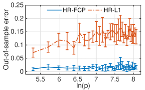
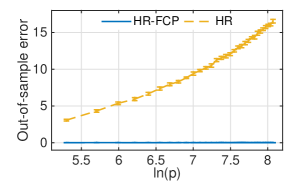
(a)	(b)
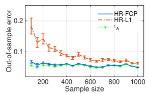
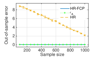
(c)	(d)
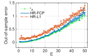
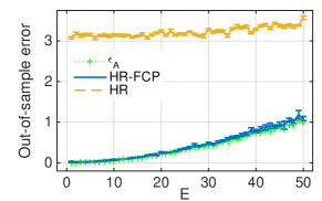
(e)	(f)
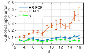
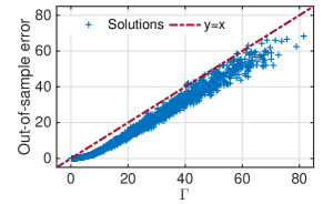
(g)	(h)

Figure 1: Numerical tests on the dependence of the out-of-sample errors in high-dimensional Huber regression on different quantities, including the logarithm of dimensionality $\ln p$ in Subplots (a)-(b), the sample size $n$ in subplots (c)-(d), the quantities $E$ and $\varepsilon_{A}$ in subplots (e)-(f), the sparsity level $s$ in subplot (g), and the underestimation of the suboptimality gap $\Gamma$ in Subplot (h). All the error bars are centered at the average levels out of 100 random replications, and the radii of the error bars are equal to 1.96 times the standard errors.

• In all the subplots CopyIn all the subplots (a) through (g) of Figure 1, blue solid lines, red dot-dashed lines, and yellow dashed lines represent the out-of-sample errors generated by the HR-FCP, the HR-L1, and the HR. The green dotted lines stand for the estimated values of $\varepsilon_{A}$, a quantity involved in the definition of A-sparsity. The values of $\varepsilon_{A}$ were estimated by (43) with $\widehat{\boldsymbol{\beta}}:={\boldsymbol{\beta}}_{\varepsilon_{A}}^{*}$. The error bars in the plot are all centered at the average levels out of 100 random replications, and the radii of the error bars are 1.96 times the corresponding standard errors.

• Subplots (a) and (b)Subplots (a) and (b) show the comparison of the HR-FCP with the HR-L1 and with the HR, respectively, when the logarithm of the dimensionality ($\ln p$) was increased gradually with $p\in\{200,300,...,5000\}$ and $E=0$. From both subplots (a) and (b), one can see that the out-of-sample errors generated by HR-FCP were small for all the values of $\ln p$, especially when the HR-FCP was compared with both the HR and the HR-L1. In particular, (as in Subplot (b)), the performance of the HR deteriorated rapidly as $\ln p$ grew, while the performance of the HR-FCP remained approximately constant. Because our error bounds for HR-FCP are polynomial in $\ln p$, it appears that an even sharper dependence on $\ln p$ may be pursued in our analysis, at least for certain HDSL special cases.

• Subplots (c) and (d)Subplots (c) and (d) present the performance of all the three schemes above when the sample size $n$ was increased from 100 to 1000 (with $E=10$ and $p=1000$). From both subplots, one can observe that the HR-FCP outperformed both the HR and the HR-L1. Also shown in these two subplots are the values of $\varepsilon_{A}$ (denoted by “$\epsilon_{A}$” in the figure). It can be observed that the out-of-sample errors of the HR-FCP matched with the values of $\varepsilon_{A}$, especially when the sample size was relatively large. This pattern was consistent with our error bounds.

• Subplots (e) and (f) CopyAs shown in Subplots (e) and (f), all the three schemes above were compared again when $E$ was increased gradually (and, as a result, $\varepsilon_{A}$ would tend to grow). Consistent with our theoretical results, the out-of-sample errors yielded by the HR-FCP approximately matched the values of $\varepsilon_{A}$ (denoted by “$\epsilon_{A}$” in the plots). Furthermore, regardless of the values of $\varepsilon_{A}$, the HR-FCP achieved better generalization errors than the HR and the HR-L1 in almost all of the instances. We can also observe from both subplots that, even if the magnitudes of the perturbation $E$ were comparable to $|\boldsymbol{\beta}_{\varepsilon_{A}}^{*}|$, the corresponding values of $\varepsilon_{A}$ remained to be small. So did the out-of-sample errors generated by the HR-FCP, especially when compared with the HR’s performance. For example, when $E=10$, the magnitude of perturbation was larger than $|\boldsymbol{\beta}_{\varepsilon_{A}}^{*}|=9.5$. Yet, the corresponding $\varepsilon_{A}$ was below 0.1, and the out-of-sample error of the HR-FCP was almost equal to $\varepsilon_{A}$. Both values were significantly lower than the corresponding out-of-sample error of the HR.

• The dependence of the HR-FCP CopyIn Subplot (g), the dependence of the HR-FCP and the HR-L1 on the sparsity level $s$ was evaluated when $E=10$, $p=1000$, $n=100$, and $\boldsymbol{\beta}_{\varepsilon_{A}}^{*}:=(3,\,5,\,0,\,0,\,1.5,\underbrace{2,\,...,2}_{\text{$(\tau)$-many 2's}},\,\leavevmode\nobreak\ \underbrace{0,\,...,0}_{\begin{subarray}{c}\text{$(p-\tau-5)$}\\ \text{-many 0's}\end{subarray}})^{\top}$ for all $\tau=0,1,...,13$. Thus, the corresponding values of $s$ were $s=3,4,...,16$. As one may see from Subplot (g), the performance of both the HR-FCP and the HR-L1 deteriorated when $s$ increased. Yet, the HR-L1 seemed to be more sensitive to the change in $s$ than the HR-FCP.

• Finally, Subplot (h) CopyFinally, Subplot (h) presents the numerical evaluation of the dependence of the HR-FCP’s out-of-sample performance on $\Gamma$. Note that, in the case of Huber regression, $\Gamma:=\left[n^{-1}\sum_{i=1}^{n}L_{HR}(\widehat{\boldsymbol{\beta}},\mathbf{x}_{i},y_{i})+\sum_{j=1}^{p}P_{\lambda}(|\widehat{\beta}_{j}|)\right]-\left[n^{-1}\sum_{i=1}^{n}L_{HR}({\boldsymbol{\beta}}^{*}_{\varepsilon_{A}},\mathbf{x}_{i},y_{i})+\sum_{j=1}^{p}P_{\lambda}(|\beta_{\varepsilon_{A},j}^{*}|)\right]$ is an underestimation of the suboptimality gap in minimizing (41). To generate this plot, we solved for the S³ONC solutions with random initialization for 2000-many repetitions. A “$+$” in the plot corresponds to one of those S³ONC solutions, and the dot-dashed line stands for the linear function of $Y=X$. If a “$+$” is below the line of $Y=X$, then it indicates that the out-of-sample error of that point was smaller than the corresponding value of $\Gamma$. As can be seen from this subplot, almost all the “+”s are below (but in the proximity of) the aforementioned linear function. This pattern was consistent with our error bound in (20), which is indeed of $\mathcal{O}(\Gamma)$ when $\Gamma\geq 1$.

7.2 Experiments on neural networks

We report two sets of experiments on the FCP-regularized NNs. The first set, as presented in this subsection, was focused on image classification using two mainstream testbeds, the MNIST (LeCun et al. 2013) and the CIFAR-10 datasets (Krizhevsky 2009). Leaderboards that report the state-of-the-art results can be found at, e.g., https://paperswithcode.com/. The second set of tests, as presented in Section 10.2 of the electronic companion, involved the comparison between the non-regularized NNs and their FCP-regularized counterparts in a task of binary classification with simulated data.

In this experiment of image classification, we considered a few popular or highly-ranked NN architectures (as well as their regularization and data augmentation schemes, if applicable), as below:

(A) For the MNIST dataset:

• CNN: A simple convolutional neural network with two convolutional layers. The codes for this model are available at https://github.com/pytorch/examples/tree/master/mnist.

• LN-S: A convolutional neural network called LeNet5 (LeCun et al. 1995) trained with a sparse learning strategy by Dettmers and Zettlemoyer (2019).

• VGG-g: A deep convolutional neural network (a.k.a., VGG8B) that is trained with global loss and cutout (DeVries and Taylor 2017) regularization. This model is presented by Nøkland and Eidnes (2019).

(B) For the CIFAR-10 dataset:

• VGG19: A deep convolutional neural network with 19 layers. The architecture was first discussed by (Simonyan and Zisserman 2014), and the codes for this network were made available by Li (2019).

• shk-RN: A residual network (He et al. 2016) with a regularization scheme that combines shake-shake (Gastaldi 2017), cutout (DeVries and Taylor 2017), and mixup (Zhang et al. 2017). The code for this network were made available by Li (2019).

• FMix (Harris et al. 2020): An NN architecture that adopts a modified mixed sample data augmentation (MSDA).

We replaced the training algorithms of the above NN implementations into Algorithm 1 with $\gamma_{opt}=10^{-6}$, using the outputs of the original implementations as the initial solutions. Some heuristic modifications were incorporated into Algorithm 1 in the above replacement: First, the gradient in Algorithm 1 was changed into an unbiased estimator of the gradient constructed on a mini-batch of the whole dataset. The mini-batch sizes remained the same as the original implementations. Second, the values of $\mathcal{M}$ could be varying over the iterations and were specified to be the multiplicative inverse for the learning rates (a.k.a., step sizes) of the original implementations. Third, $a$, the parameter in FCP, was always set to be 0.99 times the current value of $\mathcal{M}^{-1}$ at each iteration (a.k.a., epoch) during the NN training. lambda determineLast, the value of $\lambda$, the other parameter of FCP, was assigned to be $\lambda:=\mathcal{C}_{\lambda}\cdot\mathcal{U}^{-1}$ heuristically, where $\mathcal{C}_{\lambda}\geq 0$ was determined as below for each NN: We first randomly selected 10% of the training data points to construct a balanced validation set. Then, we found the 1st, 1.25th, 2.5th, 5th, 10th, and 15th percentile absolute values of the nonzero fitting parameters in the initial solution. After rounding these percentile values to their first significant digits, the resulting numbers were considered as the candidates for $\mathcal{C}_{\lambda}$. From these candidates, we then selected the one that led to the best classification result for the validation set, when the NN model was trained on the rest of the training set. As it turned out, $\mathcal{C}_{\lambda}$ was $1\times 10^{-2}$, $5\times 10^{-6}$, and $2\times 10^{-4}$, respectively, for CNN-FCP, LN-S-FCP, and VGG-g-FCP in the experiments on the MNIST dataset, and $1\times 10^{-3}$, $3\times 10^{-2}$, and $1\times 10^{-3}$, respectively, for VGG-19-FCP, shk-RN-FCP, and FMix-FCP in the experiments on the CIFAR-10 dataset.

The tests in this subsection were implemented using Pytorch (Paszke et al. 2017), and most of the tests were conducted on a single thread on a PC with 40 Intel (R) Xeon (R) E5-2640-v4 CPU cores (2.40 GHz, 64 bits), 128 GB memory, and one Quadro M4000 GPU (8GB memory), except that shk-RN and shk-RN-FCP were implemented using one GPU-enabled thread on Floydhub, a cloud computing platform with an Intel Xeon CPU (4 Cores), 61GB RAM, and an NVIDIA Tesla K80 GPU (12 GB Memory) and FMix and FMix-FCP were tested on the same cloud computing platform with different configurations (Intel Xeon CPU with 8 Cores, 61GB RAM, and an NVIDIA Tesla V100 GPU with 16 GB Memory).

The out-of-sample classification errors are reported in Tables 2 and 3 for results on MNIST and CIFAR-10, respectively. One may tell from the tables that the performance of all the NN architectures involved in the test were sharpened by incorporating the proposed FCP regularization. In particular, the best out-of-sample classification errors achieved by the FCP-regularized schemes for MNIST and CIFAR-10 were 0.23% and 1.31%, respectively, both of which were competitive against some high-performance NNs on the leaderboards (available at https://paperswithcode.com/), especially if we notice that no external data were used.

The number of nonzero fitting parameters of the NNs after training with and without the FCP are also reported in Tables 2 and 3. One may observe that the FCP significantly reduced the number of active fitting parameters. For the case of LN-S, the FCP was able to further reduce the dimensionality on top of the sparsity-inducing mechanisms in the original model.

Table 2: Classification errors of NN variants with and without the FCP on MNIST dataset. “$\langle$Model Name$\rangle$-FCP” refers to the an FCP-regularized NN. “Param #” stands for the number of nonzero fitting parameters after training. “‘R.Gap” standards for the relative gap; that is, the ratio between the difference and the value obtained before introducing the FCP.

Model	CNN	CNN-FCP	R. Gap
Test Error	0.80%	0.70%	12.50%
Param #	1,199,882	265,517	77.87%
Model	LN-S	LN-S-FCP	R. Gap
Test Error	0.66%	0.64%	3.03%
Param #	22,000*	14,417	34.47%
Model	VGG-g	VGG-g-FCP	R. Gap
Test Error	0.25%	0.23%	8.00%
Param #	16,853,584	15,115,902	10.31%

• The original LN-S model has 431,080 fitting parameters. The built-in sparsity-inducing mechanisms of the LN-S led to a model with 22,000 nonzero fitting parameters.

Table 3: Classification errors of NN variants with and without the FCP on CIFAR-10 dataset. “$\langle$Model Name$\rangle$-FCP” refers to the an FCP-regularized NN. “Param #” stands for the number of nonzero fitting parameters after training. “R.Gap” standards for the relative gap; that is, the ratio between the difference and the value obtained before introducing the FCP.

Model	VGG19	VGG19-FCP	R.Gap
Test Error	6.86%	6.84%	12.50%
Param #	20,051,546	10,789,567	46.19%
Model	shk-RN	shk-RN-FCP	R.Gap
Test Error	2.29%	2.16%	5.67%
Param #	11,932,743	7,303,200	38.79%
Model	FMix	FMix-FCP	R.Gap
Test Error	1.36%	1.31%	3.68%
Param #	26,422,068	21,485,594	18.68%

8 Conclusion

In this paper, we provide a theoretical framework for HDSL under A-sparsity; that is, the high-dimensional learning problems where the vector of the true parameters may be dense but can be approximated by a sparse vector. We show that, for a problem of this type, an S³ONC solution for an FCP-based learning formulation yields a poly-logarithmic sample complexity: the required sample size is only poly-logarithmic in the number of dimensions, even if the common assumption of the RSC is absent. To compute a solution with the proven sample complexity, we propose a novel, pseudo-polynomial-time gradient-based algorithm.

Our results on HDSL under A-sparsity can be applied to the analysis of two important learning problems that are currently less understood: (i) the nonsmooth HDSL problems, where the empirical risk functions are not necessarily differentiable; and (ii) an NN with a flexible choice of the network architectures. We show that for both problems, the incorporation of the FCP regularization can ensure the generalization performance, as measured by the excess risk, to be insensitive to the increase of the dimensionality. Particularly, our results indicate that, with regularization, an over-parameterized deep NN can be provably generalizable.

Our numerical results are consistent with our theoretical predictions and point to the interesting potential of combining the proposed FCP with some other recent techniques in further enhancing an NN’s performance. For future research, we will extend the results to other regularization schemes. weak sparsity discussionWe will also study how our results can be adapted to the analysis of HDSL under the assumption of weak sparsity (Negahban et al. 2012).

Appendices

9 Additional Results on the Neural Networks

This section of the electronic companion is focused on the generalizability of the neural networks (NN) in binary classification. The problem settings of this classification problem follow Section 6.2. Section 9.1 presents a corollary of Theorem 6.7, where quantities like $\Omega(s_{A})$ are made more explicit. Then Section 9.2 presents a suboptimality-independent generalization error bound for a ReLU-NN.

9.1 Generalizability of NNs under additional regularities.

This subsection presents a corollary of Theorem 6.7 under some additional assumptions on the separating function $g$, activation functions, and the network architecture. Below we start by introducing those assumptions.

First, we impose additional regularities on the separating function $g$ following Mhaskar (1996). Following Copy mhaskarWe let $\mathbf{D}^{\mathbf{k}}$ represent the partial derivative with order $\mathbf{k}=(k_{1},\,...,k_{d})^{\top}\geq\mathbf{0}$ and $|\mathbf{k}|=k_{1}+...+k_{d}$; that is, $\mathbf{D}^{\mathbf{k}}\widetilde{g}:=\frac{\partial^{|\mathbf{k}|}\widetilde{g}}{\partial x_{1}^{k_{1}},\cdots,\,\partial x_{d}^{k_{d}}}$, for a function $\widetilde{g}$. Define that $\mathbb{F}_{d,r}:=\left\{\widetilde{g}\in\mathbb{W}^{r,\infty}([-1,1]^{d}):\,\|\widetilde{g}\|_{\mathbb{W}^{r,\infty}([-1,1]^{d})}\leq 1\right\}.$ Here $\mathbb{W}^{r,\infty}([-1,1]^{d})$ is the Sobolev space of functions on $[-1,1]^{d}$ with continuous derivatives with order $\mathbf{r}$ for all $\mathbf{r}\in\mathbb{Z}^{d}\cap[0,r]^{d}$, where $\mathbb{Z}$ is the set of integers. Meanwhile, $\|\widetilde{g}\|_{\mathbb{W}^{r,\infty}([-1,1]^{d})}:=\sum_{\mathbf{k}\in\mathbb{Z}^{d}:\,\mathbf{k}\in[0,\,r]^{d}}\,\underset{\mathbf{x}\in[-1,1]^{d}}{\text{ess\,sup}}|\mathbf{D}^{\mathbf{k}}{\widetilde{g}}(\mathbf{x})|.$ By this definition, $\mathbb{F}_{d,r}$ is a fairly flexbile class of functions. The corollary to be presented subsequently is focused on the cases that the separating function $g$ is an element from $\mathbb{F}_{d,r}$. An important special case is where $g$ is a polynomial.

Second, we make the following assumption on the activation functions also following Mhaskar (1996): Let the activation CopyLet the activation function $\Psi$ be infinitely many times continuously differentiable in some open interval in $\Re$. Furthermore, $\frac{\partial^{k}\Psi(z)}{\partial z^{k}}\neq 0$ for some $z$ in that interval, for any integer $k\geq 0$. The same assumption CopyAccording to Mhaskar (1996), commonly adopted activation functions, such as sigmoid, hyperbolic tangent, Gaussian, and multiquadratics, all obey Assumption 9.1.

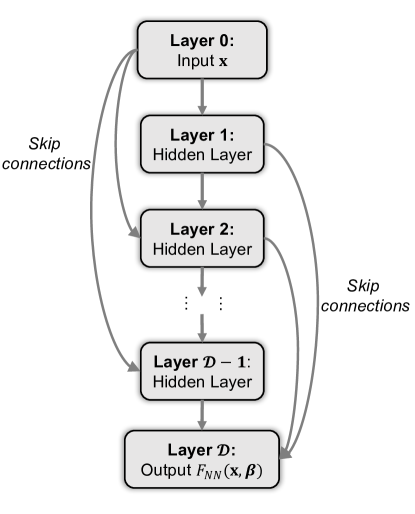
Figure 2: Illustration of the deep NN network. “Skip connections” are in presence from the input layer to hidden layers as well as from hidden layers to the output layer. No nonlinear transform is in presence in the output layer.

Third, for convenience of discussion, we focus on Copywe focus on an NN architecture as in Figure 2. In this NN, there are “skip connections” from the input layer to the $l$th hidden layer, for all $l=2,...,\mathcal{D}-1$. Meanwhile, there are also “skip connections” from the $l$ hidden layer, for all $l=1,...,\mathcal{D}-2$, to the output layer. We let $\mathcal{D}$ and $K$ be the network depth and the number of neurons in each hidden layer, respectively. Without loss of generality, we assume that all hidden layers have the same number of neurons, and all hidden neurons adopt the same activation function $\Psi$. We also assume that the output layer involves no nonlinear transformation. The output of this NN, given input $\mathbf{x}$ and fitting parameters $\boldsymbol{\beta}=vec\left((\mathbf{W}_{l-1,l}),(\mathbf{b}_{l-1,l}),\,(\boldsymbol{w}_{l,\mathcal{D}}),\,(b_{l,\mathcal{D}}),\,(\mathbf{W}_{0,l}),\,(\mathbf{b}_{0,l})\right)\in\Re^{p}$, can be captured by the nonlinear system below, where $f_{NN,l}:\Re^{d}\times\Re^{p}\rightarrow\Re^{K}$ is the output from the $l$th layer.

$$F_{NN}(\mathbf{x},\boldsymbol{\beta})= \sum_{l=1}^{\mathcal{D}-1}\left(\boldsymbol{w}_{l,\mathcal{D}}^{\top}f_{NN,l}(\mathbf{x},\boldsymbol{\beta})+b_{l,\mathcal{D}}\right);$$ (44)

$$f_{NN,l}(\mathbf{x},\boldsymbol{\beta})= \Psi\left(\mathbf{W}_{l-1,l}f_{NN,l-1}(\mathbf{x},\boldsymbol{\beta})+\mathbf{b}_{l-1,l}\right)+\Psi\left(\mathbf{W}_{0,l}\mathbf{x}+\mathbf{b}_{0,l}\right),\leavevmode\nobreak\ \leavevmode\nobreak\ \leavevmode\nobreak\ \forall l=2,...,\mathcal{D}-1;$$ (45)

$$f_{NN,1}(\mathbf{x},\boldsymbol{\beta})= \Psi\left(\mathbf{W}_{0,1}\mathbf{x}+\mathbf{b}_{0,1}\right).$$ (46)

With the foregoing settings, below is our result on the NN’s generalization error.

Corollary 9.1

Let $g\in\mathbb{F}_{d,r}$. Consider a deep neural network $F_{NN}$ defined as in (44)-(46). Suppose that Assumptions 6.2, 6.2, and 9.1 hold. Let $\widehat{\boldsymbol{\beta}}\in\Re^{p}$ be any random vector such that $\|\widehat{\boldsymbol{\beta}}\|_{\infty}\leq\frac{1}{2}v^{-1}\cdot R_{\Omega}\cdot\ln n$ and the S³ONC$(\mathbf{X},\mathbf{y})$ holds at $\widehat{\boldsymbol{\beta}}$ almost surely. For a fixed $\Gamma\geq 0$, assume that $\mathcal{T}_{n,\lambda}(\widehat{\boldsymbol{\beta}})-\inf_{{\boldsymbol{\beta}}}\mathcal{T}_{n,\lambda}({\boldsymbol{\beta}})\leq\Gamma$, w.p.1. Let $C_{7}>0$ be a universal constant and $\mathcal{C}_{NN}>0$ be some constant that depends only on $d$ and $r$. If $a<\frac{1}{2}\cdot\exp\left\{-\mathcal{U}_{NN}\cdot{\mathcal{D}}\cdot\ln\left[p\cdot v^{-1}\cdot\mathcal{U}_{NN}\cdot R_{\Omega}\cdot\ln n\right]\right\}$, $\lambda:=\sqrt{\frac{8\sigma}{c\cdot a\cdot n^{2/3}}\left[\ln(\frac{3e}{2v}\cdot R_{\Omega}pn^{4/3})+\mathcal{U}_{NN}\cdot{\mathcal{D}}\cdot\ln\left(\mathcal{U}_{NN}\cdot(1+npR_{\Omega}v^{-1})\right)\right]}$, and

$$n>C_{7}\cdot\left[\left(\mathcal{C}_{NN}\cdot v^{-1}\ln n\right)^{3d/r}+(\Gamma+1)^{3}\right]\\ +C_{7}\cdot\min\left\{\left[(d+1)\cdot{\mathcal{D}}\cdot\mathcal{U}_{NN}\cdot\ln\left(\mathcal{U}_{NN}\cdot(1+npR_{\Omega}v^{-1})\right)\right]^{3/2},\right.\\ \left.\,(d+1)\cdot K\cdot{\mathcal{D}}^{2}\cdot\mathcal{U}_{NN}\cdot\ln\left(\mathcal{U}_{NN}\cdot\left(npR_{\Omega}v^{-1}+1\right)\right)\vphantom{a^{3^{3}}}\right\},$$ (47)

then it holds that

$$\mathbb{E}\left[\mathbb{1}\left(y\cdot F_{NN}(\mathbf{x},\widehat{\boldsymbol{\beta}})<0\right)\right]\leq C_{7}\cdot\sqrt{\frac{\Gamma}{n^{1/3}}}+\frac{\mathcal{C}_{NN}^{1/2}\cdot v^{-1/2}\cdot\sqrt{\ln n}}{\min\left\{n^{\frac{1}{6}+\frac{r}{6d}},\,(K\cdot{\mathcal{D}})^{\frac{r}{2d}}\cdot n^{\frac{1}{6}}\right\}}+\Gamma\\ +\mathcal{C}_{NN}\cdot v^{-1}\cdot\max\left\{n^{-\frac{r}{3d}},\,(K\cdot{\mathcal{D}})^{-\frac{r}{d}}\right\}\cdot\ln n+C_{7}\cdot\frac{(d+1)\cdot{\mathcal{D}}\cdot\mathcal{U}_{NN}\cdot\ln\left(\mathcal{U}_{NN}\cdot(1+npR_{\Omega}v^{-1})\right)}{n^{1/3}},$$ (48)

with probability at least $1-C_{7}p\exp\left(-\frac{n}{C_{7}}\right)-C_{7}\exp\left(-\frac{n^{1/3}}{C_{7}}\right).$

Proof 9.2

Proof. See proof in Section 13.3.2. $\Box$

Remark 9.3

Below are a few remarks on Corollary 9.1.

• We attain the the poly-logarithmic sample complexity again in this corollary. Similar to Theorem 6.7, the generalization error bound in (48) is strictly monotone in the suboptimality gap $\Gamma$.

• If $g$ is a polynomial function, which is infinitely many times differentiable, and if the network is over-parameterized with $n\leq(K\mathcal{D})^{3}$, then we may as well let $d=r$ and obtain from (48) that

  $$\mathbb{E}\left[\mathbb{1}\left(y\cdot F_{NN}(\mathbf{x},\widehat{\boldsymbol{\beta}})<0\right)\right]\leq O(1)\cdot\frac{(d+1)\cdot{\mathcal{D}}\cdot\mathcal{U}_{NN}\cdot\ln\left(\mathcal{U}_{NN}\cdot(1+npR_{\Omega}v^{-1})\right)}{n^{1/3}}\\ +O(1)\cdot\sqrt{\frac{\Gamma}{n^{1/3}}}+\frac{\left(\mathcal{C}_{NN}^{1/2}+\mathcal{C}_{NN}\right)\cdot v^{-1}\cdot\ln n}{n^{1/3}}+\Gamma,$$ (49)

  with overwhelming probability.

• By a closer CopyBy a closer examination, Corollary 9.1 is obtained by explicating the misspecification error $\Omega(\cdot)$ in Theorem 6.7. In doing so, we reduce the NN defined as in (44)-(46) to a one-hidden-layer subnetwork with $(K\cdot\mathcal{D})$-many hidden neurons by assigning 0 to all the connection weights between any pair of hidden layers. We can then use the existing upper bounds on the misspecification error of a one-hidden-layer NN, such as the results by Mhaskar (1996), to provide a (conservative) estimate of $\Omega(\cdot)$. We conjecture that the same argument can be extendable to many other NN architectures, given that they can represent a one-hidden-layer subnetwork with $(K\cdot\mathcal{D})$-many hidden neurons. Here, we say that one NN (denoted by $F_{NN,1}$) can be represented by another NN (denoted by $F_{NN,2}$), if it holds that, for any $\boldsymbol{\beta}_{1}$ and almost every $\mathbf{x}\in\mathcal{X}$, $F_{NN,1}(\mathbf{x},\boldsymbol{\beta}_{1})=F_{NN,2}(\mathbf{x},\boldsymbol{\beta}_{2})$ for some $\boldsymbol{\beta}_{2}$. Because many NN architectures entail strong representability, we think that Corollary 9.1 can be used to understand a broader spectrum of NN-based models.

9.2 A suboptimality-independent generalization bound at tractable local solutions.

This subsection presents a result on the generalizability of a ReLU-NN at a pseudo-polynomial-time computable solution. Different from the above, the error bound herein is independent of the suboptimality gap $\Gamma$. This is possible under the following assumption on the data generation process. There exists a constant Copy Assumption 11There exists a constant $v\in(0,1)$ and

$$g(\cdot)\in\left\{G(\,\cdot\,):\,G(\mathbf{x})=\int_{\Re^{d}}C_{g}(\mathbf{u})\cdot\max\left\{0,\,\mathbf{u}^{\top}\mathbf{x}\right\}\cdot P(\mathbf{u})d\mathbf{u}:\,\sup_{\mathbf{u}}|C_{g}(\mathbf{u})|\leq 1\right\},$$

where $P(\mathbf{u})$ is the density of a standard Gaussian vector, such that $y\cdot g(\mathbf{x})\geq v$ for all $(\mathbf{x},\,y)\in supp(\mathbb{D})$. Assumption follows in their analysisAssumption 9.2 follows Assumption 4.10 by Cao and Gu (2020) and Assumption A.1 by Cao and Gu (2019) in their analysis on the generalization performance of the ReLU-NNs trained with a stochastic gradient descent (SGD) algorithm. The same assumption is also equivalent to the condition discussed by Rahimi and Recht (2009), for some choices of parameters, in analyzing a one-hidden-layer NN. According to Cao and Gu (2020), Assumption 9.2 holds for all the functions representable by an infinite-width one-hidden-layer ReLU-NN with a rapidly decaying second-layer weights (faster than $P(\mathbf{u})$). Because of the strong representability of an infinite-width ReLU-NN, we think that the set of functions defined in Assumption 9.2 is reasonably flexible.

Though our results can be adapted to facilitate the analysis of a more flexible class of NN architectures, we focus on a ReLU-NN architecture $F_{NN}:\,\mathcal{X}\times\Re^{p}\rightarrow\Re$ that is in accordance with the following system, given fitting parameters $\boldsymbol{\beta}=vec\left((\mathbf{W}_{l-1,l}:\,2\leq l\leq\mathcal{D}-1),(\mathbf{b}_{l-1,l}:\,2\leq l\leq\mathcal{D}-1),\,\boldsymbol{w}_{\mathcal{D}-1,\mathcal{D}},\,\boldsymbol{w}_{1,\mathcal{D}},\,,b_{\mathcal{D}-1,\mathcal{D}},\mathbf{W}_{0,1},\mathbf{b}_{0,1}\right)\in\Re^{p}$:

$$F_{NN}(\mathbf{x},\boldsymbol{\beta})= \boldsymbol{w}_{{\mathcal{D}}-1,{\mathcal{D}}}^{\top}f_{NN,{\mathcal{D}}-1}(\mathbf{x},\boldsymbol{\beta})+\boldsymbol{w}_{1,{\mathcal{D}}}^{\top}\Psi\left(\mathbf{W}_{0,1}\mathbf{x}+\mathbf{b}_{0,1}\right)+b_{{\mathcal{D}}-1,{\mathcal{D}}};$$ (50)

$$f_{NN,l}(\mathbf{x},\boldsymbol{\beta})= \Psi\left(\mathbf{W}_{l-1,l}f_{NN,l-1}(\mathbf{x},\boldsymbol{\beta})+\mathbf{b}_{l-1,l}\right),\leavevmode\nobreak\ \leavevmode\nobreak\ \leavevmode\nobreak\ \forall l=2,...,{\mathcal{D}}-1;$$ (51)

$$f_{NN,1}(\mathbf{x},\boldsymbol{\beta})= \Psi\left(\mathbf{W}_{0,1}\mathbf{x}+\mathbf{b}_{0,1}\right).$$ (52)

where we let $\Psi(z):=\max\{0,\,z\}$ be the ReLU activation function. The system in (50)-(52) captures a fully-connected ${\mathcal{D}}$-layer NN (with $\mathcal{D}-1$ hidden layers), where the first hidden layer is connected with the output layer directly through “skip connections”. We assume that there are $K$-many neurons in the every hidden layer.

In order to effectively train the above ReLU-NN, we propose the following initialization scheme (Algorithm 2) modified from the Weighted Sums of Random Kitchen Sinks (WSRKS) fitting procedure by Rahimi and Recht (2009) for training shallow networks.

  Algorithm 2. A tractable initialization scheme  

Step 0.

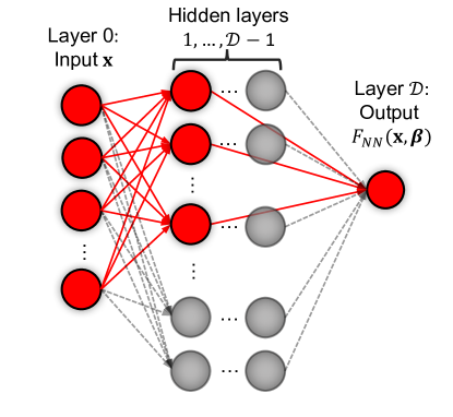
Figure 4: Illustration of the initialization scheme for training the ReLU-NN. The red nodes and links constitute the subnetwork to be initialized via Algorithm 2.

Specify an integer $K^{*}:\,1\leq K^{*}\leq K$. Consider a subnetwork in Figure 4 (where the subnetwork is highlighted in red) of the complete ReLU-NN (50)-(52). Denote this subnetwork by $F^{sub}_{NN}:\,\mathcal{X}\times\Re^{p}\rightarrow\Re$, which writes as $F^{sub}_{NN}\left(\mathbf{x},(\widetilde{\mathbf{W}}_{0,1},\,\widetilde{\boldsymbol{w}}_{1,{\mathcal{D}}})\right):=\widetilde{\boldsymbol{w}}_{1,{\mathcal{D}}}^{\top}\Psi\left(\widetilde{\mathbf{W}}_{0,1}\mathbf{x}\right)$. Here, we let $\widetilde{\mathbf{W}}_{0,1}=(\omega_{0,1,k,\iota}:\,k=1,...,K^{*},\,\iota=1,...,d)\in\Re^{K^{*}\times d}$ and $\widetilde{\boldsymbol{w}}_{1,{\mathcal{D}}}=(\omega_{1,{\mathcal{D}},k}:\,k=1,...,K^{*})\in\Re^{K^{*}}$.

Step 1.

Generate each entry of $\mathbf{W}^{initial}_{0,1}=\left((\mathbf{w}_{0,l,k}^{initial})^{\top}:\,k=1,...,K^{*}\right)$, independently, from a standard normal distribution $\mathcal{N}(0,1)$.

Step 2.

Compute $\boldsymbol{w}_{1,{\mathcal{D}}}^{initial}=\left(w^{initial}_{1,{\mathcal{D}},k}:\,k=1,...,K^{*}\right)$ by solving the following (convex) optimization problem, where all the entries of $\mathbf{W}^{initial}_{0,1}$ are fixed to be the values from Step 1:

$${\boldsymbol{w}}_{1,{\mathcal{D}}}^{initial}\in \,\underset{\|\widetilde{\boldsymbol{w}}_{1,{\mathcal{D}}}\|_{\infty}\leq n}{\arg\,\min}\,\frac{1}{n}\sum_{i=1}^{n}\mathcal{F}\left(y_{i}\cdot F^{sub}_{NN}\left(\mathbf{x}_{i},({\mathbf{W}}^{initial}_{0,1},\,\widetilde{\boldsymbol{w}}_{1,{\mathcal{D}}})\right)\right),$$ (53)

Step 3.

Let $\widehat{\boldsymbol{\beta}}^{initial}\in\Re^{p}$ be a vector of fitting parameters. Set the components of $\widehat{\boldsymbol{\beta}}^{initial}$ that correspond to the subnetwork to be $vec(\mathbf{W}^{initial}_{0,1},\,\boldsymbol{w}_{1,{\mathcal{D}}}^{initial})$. Let all other components of $\widehat{\boldsymbol{\beta}}^{initial}$ be zero.

Step 4.

Output $\widehat{\boldsymbol{\beta}}^{initial}$.

 

Algorithm 2 essentially trains the subnetwork constructed in Step 0 of Algorithm 2 with the WSRKS fitting procedure. Meanwhile, all the fitting parameters outside the subnetwork are set to be zero. Subsequent to this initialization scheme, we may then invoke Algorithm 1 to generate the desired solution to the FCP-regularized training formulation in (37).

A subtlety arises when applying Algorithm 1 to the ReLU-NN. The ReLU activation function $\Psi(z):=\max\{0,\,z\}$ is nonsmooth. Resultantly, the empirical risk function is not everywhere differentiable in general. A common approach in the literature (e.g., Berner et al. (2019)) to avoid this irregularity is to consider a modified first derivative of $\Psi$ defined as $\frac{\partial\Psi(z)}{\partial z}:=\mathbb{1}(z>0)$. By this definition, a chain rule is preserved as per Berner et al. (2019). Correspondingly, the (modified) gradient can be calculated with the detailed formula provided in Section 11. We adopt this modification in Algorithm 1. Despite the use of these modifications, we show that the combination of Algorithms 1 and 2 can lead to a generalizable ReLU-NN within pseudo-polynomial time, and the resulting sample complexity is poly-logarithmic in $p$. Furthermore, the generalization error is independent of $\Gamma$, the suboptimality gap.

Theorem 9.4 below shows the promised suboptimality-independent generalization error bound. Note that this theorem adopts the following settings and hyper-parameters:

$$\mathcal{M}>0;\quad{K^{*}}=\left\lceil 10n^{1/3}\cdot(\ln n)^{5/3}\right\rceil;\quad a<\frac{1}{\mathcal{M}};\quad\text{and}\quad\lambda:=\sqrt{\frac{8}{c\cdot a\cdot n^{2/3}}[\ln(9en^{4/3}p^{3/2}{\mathcal{D}})+{\mathcal{D}}\ln(KR)]},$$ (54)

where $K^{*}$ is defined in Algorithm 2 and $(a,\,\lambda)$ are tuning parameters of the FCP. For invoking Algorithm 1 in training the ReLU-NN, we let $\widetilde{f}(\,\cdot\,):=n^{-1}\sum_{i=1}^{n}\mathcal{F}\left(y_{i}\cdot F_{NN}(\mathbf{x}_{i},\,\cdot\,)\right)$ and $\nabla\widetilde{f}(\,\cdot\,):=n^{-1}\sum_{i=1}^{n}\widetilde{\nabla}_{\boldsymbol{\beta}}\mathcal{F}\left(y_{i}\cdot F_{NN}(\mathbf{x}_{i},\,\cdot\,)\right)$ with $\widetilde{\nabla}_{\boldsymbol{\beta}}\mathcal{F}\left(y_{i}\cdot F_{NN}(\mathbf{x}_{i},\,\cdot\,)\right)$ defined in Section 11. Finally, it is worth noting that the output of Algorithm 1 can be understood as a deterministic (and implicit) function of its initial solution $\boldsymbol{\beta}^{0}$ and training data $(\mathbf{X},\,\mathbf{y})$. When $\boldsymbol{\beta}^{0}$, $\mathbf{X}$, and $\mathbf{y}$ are random, the algorithm’s output is also a random vector.

Theorem 9.4

Consider the ReLU-NN in (50)-(52) with $K\geq\max\{2,\,d,\,10n^{1/3}\cdot(\ln n)^{5/3}+1\}$. Suppose that Assumption 9.2 holds and that $\widehat{\boldsymbol{\beta}}\in\Re^{p}$ with $\|\widehat{\boldsymbol{\beta}}\|_{\infty}\leq R$ for some $R\geq n$ is the output of Algorithm 1 when it terminates as per the stopping criterion in (26). Given hyper-parameters as in (54), the following statements hold.

• For any initial solution $\boldsymbol{\beta}^{0}\in\Re^{n}$ and training data $(\mathbf{X},\mathbf{y})$, Algorithm 1 terminates at the $k^{*}(\boldsymbol{\beta}^{0},\mathbf{X},\mathbf{y})$-th iteration, for some integer $k^{*}(\boldsymbol{\beta}^{0},\mathbf{X},\mathbf{y})<\left(\left\lceil 2\mathcal{M}\cdot\frac{\mathcal{T}_{n,\lambda}(\widehat{\boldsymbol{\beta}}^{initial})}{\gamma_{opt}^{2}}\right\rceil+1\right)$.

• Further assume that the initial solution of Algorithm 1 is the output of Algorithm 2; that is, ${\boldsymbol{\beta}}^{0}:=\widehat{\boldsymbol{\beta}}^{initial}$. At the termination of Algorithm 1, there exists a universal constant $C_{8}>0$ such that, if

  $$n>C_{8}\cdot d^{3}\cdot v^{-3}\cdot{\mathcal{D}}^{3/2}\cdot\left(\ln n\right)^{4}\cdot[\ln(pR)]^{3},$$ (55)

  then, with probability at least $1-C_{8}\cdot p\exp\left(-\frac{n^{1/3}}{C_{8}}\right)-C_{8}\cdot n^{1/3}d\exp(-n^{2}/2)-C_{8}\cdot(d\cdot n)^{-d/3}$, the generalization error of the trained ReLU-NN is bounded by

  $$\mathbb{E}\left[\mathbb{1}\left(y\cdot F_{NN}(\mathbf{x},\widehat{\boldsymbol{\beta}})<0\right)\right]\leq C_{8}\cdot\frac{d\cdot{\mathcal{D}}}{n^{1/3}v^{2}}\cdot\left[\left(\ln n\right)^{4/3}\cdot\ln(pR)\right]-\frac{\gamma^{2}_{opt}}{2\mathcal{M}}\cdot k^{*}(\widehat{\boldsymbol{\beta}}^{initial},\mathbf{X},\mathbf{y}).$$ (56)

Proof 9.5

Proof. See Section 13.3.3.

Remark 9.6

In this theorem, the generalization error bound, as measured in terms of the expected 0-1 loss, is no longer dependent on the suboptimality gap $\Gamma$, yet the promised poly-logarithmic sample complexity is maintained; the sample size should grow only poly-logarithmically to compensate for the growth in $p$. In addition, the dependence on the number of layers $\mathcal{D}$ is polynomial. In contrast to the literature, we argue that our result here may provide a significantly better rate in terms of both $p$ and ${\mathcal{D}}$, especially when considering that the training algorithm to ensure the desired sample complexity is provably in pseudo-polynomial time as per the remark below.

Remark 9.7

The combination of Algorithms 1 and 2 in Theorem 9.4 yields a pseudo-polynomial-time complexity.

• In the initialization step, Algorithm 2 is a polynomial-time algorithm. The main computational effort is on solving (53), which is convex and thus in polynomial time. (Note that an approximate solution to (53) with a suboptimality gap of $\mathcal{O}(\frac{d\cdot\mathcal{D}\cdot\ln p}{n^{1/3}})$ would actually suffice for deriving the same sample complexity as in Theorem 9.4.)

• Subsequent to Algorithm 2, Algorithm 1 computes a solution that entails the desired sample complexity. The iteration complexity of Algorithm 1, as proven in Part (a) of Theorem 9.4, is polynomial in both the dimensionality and the numeric values of the problem data. Thus, Algorithm 1 yields a pseudo-polynomial-time complexity.

With the above, we know that the total computational effort of the combined algorithm is in pseudo-polynomial time.

Remark 9.8

The proof of Theorem 9.4 does not depend on how the gradient is defined or modified. Nonetheless, there is some benefit of using the “modified gradient” as in Section 11, as discussed in Remark 9.9 below.

Remark 9.9

By a closer examination of the proof, one may notice that Algorithm 2 (invoked for initialization) alone is already capable of identifying a solution with provable generalizability. Nonetheless, as per (56), Algorithm 1 sharpens the generalization error; the more iterations that Algorithm 1 would run for, the shaper is the performance of the trained NN. A natural question would be whether the initial solution identified by Algorithm 2 would render the stoping criterion in (26) to be satisfied at the first iteration of Algorithm 1. If so, $k^{*}(\widehat{\boldsymbol{\beta}}^{initial},\mathbf{X},\mathbf{y})=0$ and Algorithm 1 would not be effective. We think it to be a possible scenario for some problem instances. However, because $\frac{1}{n}\sum_{i=1}^{n}\mathcal{F}(y_{i}\cdot F_{NN}(\mathbf{x}_{i},\cdot))$ is a piecewise smooth function and Algorithm 2 trains only a small subset of the fitting parameters, it is more likely that the initial solution generated by Algorithm 2 is a non-KKT point within a continuously differentiable neighborhood. In such a case, the “modified gradient” as in Section 11 becomes the exact formulation of the gradient. One may then show that $k^{*}(\widehat{\boldsymbol{\beta}}^{initial},\mathbf{X},\mathbf{y})>0$ must hold, if $\mathcal{M}$ is properly large and greater than the Lipschitz constant of the gradient of $\frac{1}{n}\sum_{i=1}^{n}\mathcal{F}(y_{i}\cdot F_{NN}(\mathbf{x}_{i},\cdot))$ for every $\boldsymbol{\beta}$ in that neighborhood.

Remark 9.10

The results of Theorem CopyThe results of Theorem 9.4 is obtained via a similar argument as in proving Theorem 6.7, except that the misspecification error $\Omega(\cdot)$ and the suboptimality gap $\Gamma$ in Theorem 6.7 are now explicated in Theorem 9.4 under the specific assumptions made on the neural network and the data generating process. To make explicit both $\Omega(\cdot)$ and $\Gamma$, our proofs are largely focused on analyzing the subnetwork constructed in Step 0 of Algorithm 2 and illustrated in Figure 4. The misspecification error of this subnetwork serves as a conservative estimate of $\Omega(\cdot)$, and the suboptimality gap obtained after training this subnetwork becomes an overestimate of the initial suboptimality gap to bound $\Gamma$. We conjecture that the above argument can be extended to any NN architecture that contains, or can represent, the above subnetwork. Such NN architectures include the conventional ReLU networks and the residual networks with ReLU activation, among others.

10 Additional Numerical Experiments

This part of the electronic companion presents some additional numerical experiments. Sections 10.1 and 10.2 below are focused on a high-dimensional SVM and a ReLU-NN, respectively.

10.1 Experiments on high-dimensional SVM

This section presents our experiments on high-dimensional SVM, whose training formulation entails a nonsmooth statistical loss function. For each experimental instance, a training set and a test set were randomly generated in two different cases below: (a) The first case involved data with less correlated design. With the same notations as in (33), let $\mathbf{x}_{1},\,\mathbf{x}_{2},\,...,\,\mathbf{x}_{n}$ be i.i.d. samples of $\mathcal{N}_{p}(\mathbf{0},\Sigma)$ with $\Sigma=(\varsigma_{j_{1},j_{2}})$ and $\varsigma_{j_{1},j_{2}}=0.3^{|j_{1}-j_{2}|}$. Let the class labels of the samples $y_{i},\,i=1,...,n$, be determined by $y_{i}=+1$ if $\mathbf{x}^{\top}_{i}\boldsymbol{\beta}^{*}+\omega_{i}\geq 0$, and $y_{i}=-1$, otherwise. Here, $\omega_{1},\,\omega_{2},...,\,\omega_{n}$ are i.i.d.  standard normal random variables and $\boldsymbol{\beta}^{*}=(3,\,5,\,0,\,0,\,1.5,\underbrace{0,\,...,0}_{\text{$(p-5)$-many 0's}})^{\top}$. We let $n=100$ for both the training and test sets. (b) In the second case, data with more correlated design were generated. In doing so, the same approach as in the first case above was followed, except that $\Sigma=(\varsigma_{j_{1},j_{2}})$ was simulated differently. We first calculated $\varsigma_{j_{1},j_{2}}=0.3^{|j_{1}-j_{2}|}$ and then shrank all the singular values of $\Sigma$ below the 80th percentile to be 0.01 times their original values.

Linear classifiers were trained on the training data via three different schemes to be explained subsequently. Their performance was measured by the out-of-sample classification error on the test data, calculated as $\frac{\text{Number of wrongly classified observations}}{\text{Total number of observations}}\times 100\%$.

Our numerical comparisons involved the following schemes: (i). SVM: The canonical SVM in (33) with $\rho=0$. (ii) SVM-$\ell_{2}$: The SVM with $\ell_{2}$ regularization, that is, the estimator generated by solving (33) with $\rho>0$. (iii) SVM-$\ell_{1}$: The SVM variant with $\ell_{1}$ regularization, that is, the estimator generated by solving (35) with $\rho=0$, and $\widetilde{P}_{\lambda}(|\cdot|)=\lambda|\,\cdot\,|$. (iv) SVM-FCP: The SVM variant with the proposed FCP-based regularization, that is, the estimator generated by solving for an S³ONC solution via Algorithm 1 to Problem (34) with $\rho=0$. Note that Algorithm 1 in (iv) was initialized with solutions generated by the SVM-$\ell_{1}$. Hyper-parameters of Algorithm 1 was specified as $\gamma_{opt}=10^{-5}$ and $\mathcal{M}=3.5\geq n^{1/4}$. The SVM, the SVM-$\ell_{2}$, and the SVM-$\ell_{1}$ were all solved by calling Mosek (ApS 2015) through CVX (Grant and Boyd 2013, 2008).

In determining copyIn determining the hyper-parameters, namely, $\rho$ in the SVM-$\ell_{2}$, $\lambda$ in the SVM-$\ell_{1}$ as well as $\lambda$ in the SVM-FCP (where we fixed the value of $a$, the other tuning parameter of the FCP, to be 0.3), three training sets with $p\in\{100,\,500,\,1000\}$ and $n=100$ were generated as per the above data generation process in the first case (with less correlated design). On these data sets, the SVM-$\ell_{2}$, the SVM-$\ell_{1}$, and the SVM-FCP models were then trained for fixed hyper-parameters, $\lambda$ or $\rho$, chosen from $\{0.05,\,0.1,\,0.15,\,0.20,...,0.4\}$. The trained SVM variants were then evaluated in terms of their classification errors on three validation sets, one for each value of $p\in\{100,\,500,\,1000\}$. These validation sets were generated with the same sample sizes and probability distributions as the three training datasets above. From the pool of candidate values for $\lambda$ and $\rho$, the best ones were chosen in terms of minimizing the average classification errors on the validation sets over all the three cases of $p=100,\,500,\,1000$. It turned out that $\lambda=0.25$ for both the SVM-FCP and the SVM-$\ell_{1}$, and $\rho=0.1$ for the SVM-$\ell_{2}$.

In testing the impact of dimensionality on the out-of-sample performance of all the four SVM variants, $p$ was increased gradually with values chosen from $\{100,\,200,\,...,1000\}$. For each choice of dimensionality, 100 random replications were conducted. The performance of each SVM variant is reported in Tables 4 and 5, where we compare the averages and standard errors of the out-of-sample classification errors for the cases with lower and higher correlations in the design, respectively. From both tables, one can see that the classification errors generated by the proposed SVM-FCP were noticeably better than all other alternative approaches involved in this test. A representation of the comparisons are provided in the two subplots of Figure 3, where the center and radius of each of the error bars are the average classification error and 1.96 times the corresponding standard error, respectively, from the 100 replications. This figure shows that the SVM-FCP persistently outperformed the other three SVM variants involved in the test.

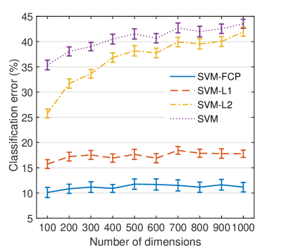
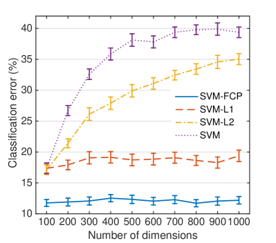
figures SVM (a) (b)

Figure 3: Comparison of classification errors (%) incurred by the SVM variants. Subplot (a) shows the case with less correlated design and Subplot (b) presents the case with more correlated design. “SVM-FCP”, “SVM-L1”, “SVM-L2”, “SVM” refers to the SVM variants with the FCP regularization, the $\ell_{1}$ regularization, the $\ell_{2}$ regularization, and no regularization, respectively. Centers of error bars are the mean classification errors out of 100 random replications, and the radius of the error bars are 1.96 times the standard errors.

Table 4: Classification errors of SVM with different regularization schemes when the design has lower correlation. “Mean” stands for the average out-of-sample classification error (%) out of 100 random replications, and “SE” is the corresponding standard error (%).

	SVM-FCP			SVM-$\ell_{1}$			SVM-$\ell_{2}$			SVM
$p$	Mean	SE		Mean	SE		Mean	SE		Mean	SE
$100$	10.11	0.26		15.73	0.28		25.76	0.28		35.36	0.25
$200$	10.83	0.24		17.21	0.22		31.69	0.24		38.06	0.28
$300$	11.17	0.28		17.54	0.28		33.63	0.22		39.01	0.21
$400$	10.91	0.20		16.93	0.22		36.83	0.24		40.49	0.25
$500$	11.75	0.26		17.65	0.26		38.18	0.26		41.52	0.26
$600$	11.69	0.29		16.89	0.23		37.75	0.24		40.67	0.24
$700$	11.50	0.28		18.44	0.19		39.91	0.24		42.72	0.25
$800$	11.15	0.26		17.87	0.21		39.56	0.27		42.00	0.27
$900$	11.63	0.27		17.82	0.24		40.02	0.25		42.55	0.24
$1000$	11.16	0.24		17.77	0.19		41.95	0.23		43.53	0.23

Table 5: Classification errors of SVM with different regularization schemes when the design has higher correlation. “Mean” stands for the average out-of-sample classification error (%) out of 100 random replications, and “SE” is the corresponding standard error (%).

additional table SVM-FCP SVM-$\ell_{1}$ SVM-$\ell_{2}$ SVM $p$ Mean SE Mean SE Mean SE Mean SE 100 11.76 0.55 17.36 0.78 17.13 0.78 17.36 0.86 200 11.91 0.65 17.91 0.78 21.41 0.73 26.71 0.82 300 12.08 0.64 19.06 0.99 26.13 1.03 32.59 0.85 400 12.53 0.58 19.14 0.93 27.90 1.01 35.86 0.97 500 12.34 0.67 18.72 0.94 29.90 1.00 38.12 1.00 600 12.05 0.62 18.84 0.94 31.09 0.93 37.82 0.97 700 12.29 0.65 19.08 0.89 32.44 0.77 39.37 0.86 800 11.71 0.58 18.63 0.80 33.43 0.86 39.78 0.79 900 12.06 0.67 18.29 0.90 34.58 1.06 39.89 1.00 1000 12.19 0.60 19.38 0.92 35.04 0.88 39.37 0.85

10.2 Numerical Experiments on ReLU-NN in Binary classification

This subsection presents our numerical tests on the efficacy of the FCP-based regularization on a ReLU-NN. A training set, a validation set, and a test set were generated as below: (A) Training set: 2000 data were first generated in line with Assumption 9.2, where $d=10$ and $C_{g}({\bf u}):=\sin({{\sum_{\iota=1}^{d}{u_{\iota}}}})/d$ with $\mathbf{u}=(u_{\iota})$. For the given $C_{g}$, (the integration involved in defining) the separating function $g(\mathbf{x})$ was evaluated via numerical integration. For each sample data with feature values $\mathbf{x}_{i}$, the corresponding (actual) label $y_{i}$ was set to be +1 if $g(\mathbf{x})\geq 0$, and $-1$, otherwise. Some mislabels were introduced. Specifically, out of these 2000-many data, a subset of data points was selected as per a Bernoulli distribution; each data point was selected with probability 0.05. All the data points in this subset were assigned the wrong labels (opposite to their actual labels calculated previously).(B) Validation set: Following the same approach as the above, we generated another set of 2000 validation data. (C) Test set: A set of 5000 independent test data were generated following Assumption 9.2, with the same $d$, $C_{g}$, and $g$ as the above. However, no test data was mislabeled.

We followed (50)-(52) in constructing the architecture of a $\mathcal{D}$-layer ReLU-NN model, where the width $K$ (i.e., the number of hidden neurons per hidden layer) was identical across all the hidden layers. We employed Algorithm 1, initialized by Algorithm 2, in training the FCP-regularized ReLU-NN formulated in Eq. (37). In choosing the hyper-parameters, we set $a=0.5$ and $\lambda=\mathcal{C}_{fcp}\cdot\mathcal{D}\cdot\sqrt{\ln K}$. Here, $\mathcal{C}_{fcp}=0.001$ was determined through a process to be detailed subsequently. For Algorithm 1, we let $\gamma_{opt}=10^{-6}$ and $\mathcal{M}=1$ (such that $a<\frac{1}{\mathcal{M}}$). For Algorithm 2, ${K^{*}}=\left\lceil 10n^{1/3}\cdot(\ln n)^{5/3}\right\rceil$ as per Theorem 9.4.

To determine $\mathcal{C}_{fcp}$, three ReLU-NN architectures with 10, 50, and 100 hidden layers and $K=150$ were trained with the combination of Algorithms 1 and 2, when $\mathcal{C}_{fcp}$ was fixed at each of the candidate values from the set $\{0.0001,\,0.0005,\,0.001,\,0.005,\,0.01,\,0.05,\,0.1\}$. The performance of these trained ReLU-NNs was evaluated on the validation set in terms of the classification errors. Then, for each candidate value of $\mathcal{C}_{fcp}$, an classification error over all the three NN architectures above was calculated. The value of $\mathcal{C}_{fcp}$ was chosen to be the one that led to the best average performance. It turned out that $\mathcal{C}_{fcp}=0.001$.

Involved as a benchmark in the experiment was the ReLU-NN model generated by solving the conventional training formulation given as

$$\inf_{\boldsymbol{\beta}}\leavevmode\nobreak\ \mathcal{T}_{n,\lambda}(\boldsymbol{\beta}):=n^{-1}\sum_{i=1}^{n}\mathcal{F}\left(y_{i}\cdot F_{NN}(\mathbf{x}_{i},\boldsymbol{\beta})\right).$$ (57)

In computing a solution to this problem, we employed an SGD algorithm based on Cao and Gu (2019), who have shown the generalizability of the ReLU-NNs trained by an SGD in spite of the nonconvexity of the formulation. The SGD in our experiment was integrated with a three-step multi-start strategy: In Step 1, we repeated, for five times, the training of the same ReLU-NN using the conventional SGD with the He initialization (He et al. 2015). Because both the He initialization and the SGD are stochastic, five potentially different local solutions could be generated by Step 1. In Step 2, we trained the ReLU-NN using the conventional SGD again, but the initial point was specified as the output of Algorithm 2. Finally, in Step 3, we compared all the solutions from Steps 1 and 2 and chose the solution with the smallest objective value (in terms of (57)) as the output of this multi-start strategy. While there could be different strategies in the literature to boost the performance of the SGD, such as a wise determination of the batch size, the momentum, and the learning rate (i.e., the step size), we did not employ those strategies; our purpose was to compare the non-regularized ReLU-NN formulation in (57) with the proposed FCP-regularized ReLU-NN. Thus, given that the SGD well optimized the problem in (57) globally, the performance of the resulting solutions were considered to well represent the efficacy of the non-regularized ReLU-NN. Indeed, in evaluating the Copyin evaluating the optimization quality of the SGD, we found that the average, maximal, and minimal objective function values out of all the numerical instances were 0.0013, 0.0052, and 0.0000, respectively. (In contrast, the average initial objective value of all the SGD runs in this experiment was 19.3101.) In view of the fact that $\inf_{u}\mathcal{F}(u)\geq 0$, we claim that the global optimal solutions to (57) were well approximated, if not always achieved, by the above SGD scheme.

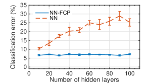
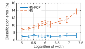
(a)	(b)
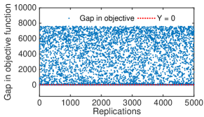
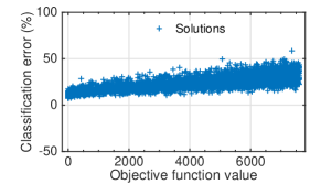
(c)	(d)

Figure 5: Numerical evaluation of the FCP-regularized NN (referred to as the NN-FCP): (a) Comparison between the NN-FCP and the non-regularized NN (referred to as the NN) when the number of hidden layers grew; (b) Comparison between the NN-FCP and the NN when the logarithm of the width of each hidden layer (that is, $\ln K$) increased; (c) Comparison between the objective function values of 5000 randomly generated solutions and that of the solution generated by combining Algorithms 1 and 2; (d) Evaluation of the dependence between in-sample training error and the out-of-sample performance. All the error bars are centered at the average levels out of 10 random replications and radii are equal to 1.96 times the standard errors.

Our numerical results are presented in Figure 5. Some discussions on this figure are as below.

• Subplot (a) of Figure 5 reports the out-of-sample classification errors of the FCP-regularized ReLU-NN and the non-regularized ReLU-NN (referred to as the NN-FCP and the NN, respectively, in the figure) when the width was fixed at $K=150$, and the number of hidden layers was chosen from a pool of candidate values $\{10,20,...,150\}$. For each combination of width and depth, we replicated the experiment for ten times. The center and the radius of each error bar in the plot are the average classification error and 1.96 times the corresponding standard error out of the ten replications. One can see that the performance of the FCP-regularized ReLU-NN was significantly better than the non-regularized ReLU-NN. Meanwhile, the performance of the former was insensitive to the growth in the depth of the network. This pattern was consistent with Theorem 9.4, but it also may have identified room for further improvement in terms of the dependence on $\mathcal{D}$, at least for some regions of the hyper-parameters.

• Subplot (b) of Figure 5 shows the out-of-sample classification errors of the FCP-regularized ReLU-NN and the non-regularized ReLU-NN when the number of hidden layers was fixed to be two and the width of the hidden layers was set to be $K\in\{150,\,200,\,250,\,300,\,350,\,400,\,450,\,500,\,750,\,1000,\,1500\}$. Note that the number of fitting parameters $p$ is polynomial in $K$. In order to show the dependence of the generalization performance on $\ln p$, the X-axis of Subplot (b) is on $\ln K$. We can see from this subplot that the performance of the FCP-regularized ReLU-NN remained almost constant as $\ln K$ increased. In contrast, the non-regularized ReLU-NN deteriorated significantly when $\ln K$ became larger.

• To show how well the FCP CopyTo show how well the FCP-regularized ReLU-NN training formulation was optimized in our experiments through the combination of Algorithms 1 and 2, we present in Subplot (c) of Figure 5 a test on the ReLU-NN with 100 hidden layers and 150 neurons per hidden layer — the largest network among all the ReLU-NNs involved in (i) and (ii) above. For this model, we generated 5000 random solutions to (37) and compared their objective function values (in terms of (37)) with that of the solution $\widehat{\boldsymbol{\beta}}\in\Re^{p}$ computed by combining Algorithms 1 and 2 as above. The $m$th (for all $m\in\{1,...,5000\}$) random solution was generated as per the following two-step process: Step 1. We generated a random vector $\mathbf{v}^{1}_{m}:=\widehat{\boldsymbol{\beta}}+\nu_{m}$, where $\nu_{m}\in\Re^{p}$ was a random sample of a centered Gaussian random vector with i.i.d. entries. The covariance matrix of each $\nu_{m}$ was prescribed to be $mod(m,\,25)\cdot R_{m}\cdot I$, where $mod(m,\,25)$ is the remainder of the Euclidean division of $m$ by $25$, $R_{m}$ denotes a uniformly distributed random number on (0, 1), and $I$ stands for the identity matrix. Step 2. For all $m=1,...,5000$, we invoked Algorithm 1 to generate a new solution $\mathbf{v}^{2}_{m}\in\Re^{p}$ using $\mathbf{v}^{1}_{m}$ as the initial point. Here, Algorithm 1 was terminated whenever either the stopping criterion in (26) was met ($\gamma_{opt}=10^{-6}$ and $\mathcal{M}=1$) or a maximal iteration number of 15 was reached. Of all these random solutions, if any could entail a smaller objective value (w.r.t. the objective function in (37)) than $\widehat{\boldsymbol{\beta}}$, then it would mean that $\widehat{\boldsymbol{\beta}}$ was not the global minimizer. A blue point in Subplot (c) of Figure 5 represents one of those random solutions. The corresponding Y-axis of that point indicates the difference between the objective values of $\mathbf{v}^{2}_{m}$ and $\widehat{\boldsymbol{\beta}}$. One may observe from the plot that, for all $m=1,...,5000$, the gaps in the objective were always above zero. This indicates that $\widehat{\boldsymbol{\beta}}$ well approximated, if not coincided with, a globally minimal solution to (37).

• In Subplot (d) of Figure 5, we reorganized data from (iii) above to show the correspondence between the in-sample training errors and the out-of-sample errors. More specifically, we sorted the random solutions $\mathbf{v}^{2}_{m}$ in the ascending order of their objective values (w.r.t. the objective function in (37)) and showed in this subplot the corresponding out-of-sample classification errors of those solutions. In the subplot, each blue “$+$” represents one of the random solutions $\mathbf{v}_{m}^{2}$. The X- and Y-axis values at the center of each “$+$” are the corresponding objective function value and the out-of-sample error, respectively. One may observe that these “$+$”s tend to cluster around an affine function.

Finally, it is worth noting that Algorithm 1 (which was initialized by Algorithm 2) always ran for more than one iteration in all the test instances. If we combine this observation with Remark 9.9 about Theorem 9.4, we then know that $k^{*}(\widehat{\boldsymbol{\beta}}^{initial},\mathbf{X},\mathbf{y})>0$ (where $k^{*}(\widehat{\boldsymbol{\beta}}^{initial},\mathbf{X},\mathbf{y})$ is defined as in Theorem 9.4) and, hence, Algorithm 1 was indeed effective in our test.

11 The “modified gradient” of the ReLU-NN

In using Algorithm 1 to train the ReLU-NN of consideration, we follow the commonly adopted definition (e.g., by Berner et al. (2019)) of the (modified) gradient (denoted by $\widetilde{\nabla}_{\boldsymbol{\beta}}\mathcal{F}(yF_{NN}(\mathbf{x},\boldsymbol{\beta}))$) of the training formulation. In this definition, we denote that $\mathcal{H}(\mathbf{v}):=diag\left(\mathbb{1}(v_{1}>0),\,\mathbb{1}(v_{2}>0),...\right)$, for any vector $\mathbf{v}=(v_{1},v_{2},...)^{\top}$. More specifically, we let $\widetilde{\nabla}_{\boldsymbol{\beta}}\mathcal{F}(yF_{NN}(\mathbf{x},\boldsymbol{\beta})):=\left.\frac{d\mathcal{F}(t)}{dt}\right|_{t=y\cdot F_{NN}(\mathbf{x},\boldsymbol{\beta}))}\cdot y\cdot\frac{\widetilde{d}F_{NN}(\mathbf{x},\boldsymbol{\beta})}{\widetilde{d}\boldsymbol{\beta}}$, where the formula for the components of $\frac{\widetilde{d}F_{NN}(\mathbf{x},\boldsymbol{\beta})}{\widetilde{d}\boldsymbol{\beta}}=\left(\frac{\widetilde{\partial}F_{NN}(\mathbf{x},\boldsymbol{\beta})}{\widetilde{\partial}\beta_{j}}:\,j=1,...,p\right)$ are given below:

$$\frac{\widetilde{\partial}F_{NN}(\mathbf{x},\boldsymbol{\beta})}{\widetilde{\partial}\boldsymbol{w}_{\mathcal{D}-1,\mathcal{D}}}:=f_{NN,\mathcal{D}-1}(\mathbf{x},\boldsymbol{\beta}),\leavevmode\nobreak\ \leavevmode\nobreak\ \leavevmode\nobreak\ \frac{\widetilde{\partial}F_{NN}(\mathbf{x},\boldsymbol{\beta})}{\widetilde{\partial}b_{\mathcal{D}-1,\mathcal{D}}}:=\mathbf{1},\leavevmode\nobreak\ \leavevmode\nobreak\ \leavevmode\nobreak\ \text{and}\leavevmode\nobreak\ \leavevmode\nobreak\ \leavevmode\nobreak\ \frac{\widetilde{\partial}F_{NN}(\mathbf{x},\boldsymbol{\beta})}{\widetilde{\partial}\boldsymbol{w}_{1,\mathcal{D}}}:=\Psi(\mathbf{W}_{0,1}\mathbf{x}+\mathbf{b}_{0,1}).$$

Meanwhile,

$$\frac{\widetilde{\partial}F_{NN}(\mathbf{x},\boldsymbol{\beta})}{\widetilde{\partial}\mathbf{W}_{l-1,l}}:=\mathcal{H}\left(\mathbf{W}_{l-1,l}f_{NN,l-1}(\mathbf{x},\boldsymbol{\beta})+\mathbf{b}_{l-1,l}\right)\cdot\mathbf{W}_{l,l+1}^{\top}\cdot\mathcal{H}\left(\mathbf{W}_{l,l+1}f_{NN,l}(\mathbf{x},\boldsymbol{\beta})+\mathbf{b}_{l,l+1}\right)\cdot...\\ \cdot\mathbf{W}_{\mathcal{D}-2,\mathcal{D}-1}^{\top}\cdot\mathcal{H}\left(\mathbf{W}_{\mathcal{D}-2,\mathcal{D}-1}f_{NN,\mathcal{D}-2}(\mathbf{x},\boldsymbol{\beta})+\mathbf{b}_{\mathcal{D}-2,\mathcal{D}-1}\right)\cdot\boldsymbol{w}_{\mathcal{D}-1,\mathcal{D}}\cdot\left[f_{NN,l-1}(\mathbf{x},\boldsymbol{\beta})\right]^{\top},\leavevmode\nobreak\ \leavevmode\nobreak\ \leavevmode\nobreak\ \text{for all $l:\,2\leq l\leq\mathcal{D}-1$};$$ (58)

$$\frac{\widetilde{\partial}F_{NN}(\mathbf{x},\boldsymbol{\beta})}{\widetilde{\partial}\mathbf{b}_{l-1,l}}:=\mathcal{H}\left(\mathbf{W}_{l-1,l}f_{NN,l-1}(\mathbf{x},\boldsymbol{\beta})+\mathbf{b}_{l-1,l}\right)\cdot\mathbf{W}^{\top}_{l,l+1}\cdot\mathcal{H}\left(\mathbf{W}_{l,l+1}f_{NN,l}(\mathbf{x},\boldsymbol{\beta})+\mathbf{b}_{l,l+1}\right)\cdot...\\ \cdot\mathbf{W}^{\top}_{\mathcal{D}-2,\mathcal{D}-1}\cdot\mathcal{H}\left(\mathbf{W}_{\mathcal{D}-2,\mathcal{D}-1}f_{NN,\mathcal{D}-2}(\mathbf{x},\boldsymbol{\beta})+\mathbf{b}_{\mathcal{D}-2,\mathcal{D}-1}\right)\cdot\boldsymbol{w}_{\mathcal{D}-1,\mathcal{D}},\leavevmode\nobreak\ \leavevmode\nobreak\ \leavevmode\nobreak\ \text{for all $l:\,2\leq l\leq\mathcal{D}-1$};$$ (59)

$$\frac{\widetilde{\partial}F_{NN}(\mathbf{x},\boldsymbol{\beta})}{\widetilde{\partial}\mathbf{W}_{0,1}}:=\mathcal{H}\left(\mathbf{W}^{\top}_{0,1}\mathbf{x}+\mathbf{b}_{0,1}\right)\cdot\mathbf{W}^{\top}_{1,2}\cdot\mathcal{H}\left(\mathbf{W}^{\top}_{1,2}f_{NN,1}(\mathbf{x},\boldsymbol{\beta})+\mathbf{b}_{1,2}\right)\cdot...\\ \cdot\mathbf{W}^{\top}_{\mathcal{D}-2,\mathcal{D}-1}\cdot\mathcal{H}\left(\mathbf{W}^{\top}_{\mathcal{D}-2,\mathcal{D}-1}f_{NN,\mathcal{D}-2}(\mathbf{x},\boldsymbol{\beta})+\mathbf{b}_{\mathcal{D}-2,\mathcal{D}-1}\right)\cdot\boldsymbol{w}_{\mathcal{D}-1,\mathcal{D}}\mathbf{x}^{\top}+\mathcal{H}\left(\mathbf{W}_{0,1}\mathbf{x}+\mathbf{b}_{0,1}\right)\cdot\boldsymbol{w}_{1,\mathcal{D}}\cdot\mathbf{x}^{\top};$$ (60)

$$\frac{\widetilde{\partial}F_{NN}(\mathbf{x},\boldsymbol{\beta})}{\widetilde{\partial}\mathbf{b}_{0,1}}:=\mathcal{H}\left(\mathbf{W}_{0,1}\mathbf{x}+\mathbf{b}_{0,1}\right)\cdot\mathbf{W}^{\top}_{1,2}\cdot\mathcal{H}\left(\mathbf{W}_{1,2}f_{NN,1}(\mathbf{x},\boldsymbol{\beta})+\mathbf{b}_{1,2}\right)\cdot...\\ \cdot\mathbf{W}^{\top}_{\mathcal{D}-2,\mathcal{D}-1}\cdot\mathcal{H}\left(\mathbf{W}_{\mathcal{D}-2,\mathcal{D}-1}f_{NN,\mathcal{D}-2}(\mathbf{x},\boldsymbol{\beta})+\mathbf{b}_{\mathcal{D}-2,\mathcal{D}-1}\right)\cdot\boldsymbol{w}_{\mathcal{D}-1,\mathcal{D}}+\mathcal{H}\left(\mathbf{W}_{0,1}\mathbf{x}+\mathbf{b}_{0,1}\right)\cdot\boldsymbol{w}_{1,\mathcal{D}}.$$ (61)

The above calculation can be conducted via back-propagation. The function $\mathcal{F}(yF_{NN}(\mathbf{x},\cdot))$ is piecewise continuously differentiable. At points where the gradient is well-defined, the above calculation equals to the gradient exactly.

12 The Applicability of Theorem 6.2 to the high-dimensional SVM

This section discusses how Theorem 6.2 can be used to analyze the generalization performance of SVM. In particular, we determine here the proper values of $R$, $\sigma$, $\sigma_{L}$, and $\mathcal{C}_{\mu}$ in the instantiation of Assumptions 6.1 and 6.1. We start by introducing a few short-hand notations. Let $\mathbf{X}=(\mathbf{x}^{\top}_{i}:\,i=1,...,n)$, $\mathbf{y}=(y_{i})$,

$$\widetilde{\mathcal{L}}^{SVM}_{n}(\boldsymbol{\beta},(\mathbf{X},\mathbf{y})):= \,\rho\|\boldsymbol{\beta}\|^{2}+\frac{1}{n}\sum_{i=1}^{n}\max_{u_{i}:\,0\leq u_{i}\leq 1}\,\left\{u_{i}\cdot\left(1-y_{i}\mathbf{x}_{i}^{\top}\boldsymbol{\beta}\right)\right\},$$

$$\widetilde{\mathcal{L}}^{SVM}_{n,\delta}(\boldsymbol{\beta},(\mathbf{X},\mathbf{y})):= \,\rho\|\boldsymbol{\beta}\|^{2}+\frac{1}{n}\sum_{i=1}^{n}\max_{u_{i}:\,0\leq u_{i}\leq 1}\,\left\{u_{i}\cdot\left(1-y_{i}\mathbf{x}_{i}^{\top}\boldsymbol{\beta}\right)-\frac{(u_{i}-u_{0})^{2}}{2n^{\delta}}\right\},\leavevmode\nobreak\ \leavevmode\nobreak\ \leavevmode\nobreak\ \leavevmode\nobreak\ \leavevmode\nobreak\ \leavevmode\nobreak\ \leavevmode\nobreak\ \leavevmode\nobreak\ \leavevmode\nobreak\ \text{and}$$

$$\widetilde{\mathcal{L}}^{SVM}_{n,\delta,\lambda}(\boldsymbol{\beta},(\mathbf{X},\mathbf{y})):= \,\rho\|\boldsymbol{\beta}\|^{2}+\frac{1}{n}\sum_{i=1}^{n}\max_{u_{i}:\,0\leq u_{i}\leq 1}\left\{u_{i}\cdot\left(1-y_{i}\mathbf{x}_{i}^{\top}\boldsymbol{\beta}\right)-\frac{(u_{i}-u_{0})^{2}}{2n^{\delta}}\right\}+\sum_{j=1}^{p}P_{\lambda}(|\beta_{j}|).$$

We first determine $R$ for the case of SVM. Observe that $\inf_{\boldsymbol{\beta}}\mathbb{E}[L_{ns}(\boldsymbol{\beta},Z_{i})]\leq\mathbb{E}[L_{ns}(\mathbf{0},Z_{i})]=1$ and $\boldsymbol{\beta}^{*}\in\arg\,\inf_{\boldsymbol{\beta}}\mathbb{E}[L_{ns}(\boldsymbol{\beta},Z_{i})]$. Recall that we have let $\rho=0.01$. Therefore, $\rho\|\boldsymbol{\beta}^{*}\|^{2}\leq 1\Longrightarrow\|\boldsymbol{\beta}^{*}\|\leq 10$. If $\boldsymbol{\beta}^{*}$ is dense and entails A-sparsity (in Assumption 1), there must exist a sparse $\boldsymbol{\beta}^{*}_{\varepsilon_{A}}\in[-10,\,10]^{p}$ that approximates $\boldsymbol{\beta}^{*}$ in the sense of Assumption 1 by the continuity of $\mathbb{E}[L_{ns}(\,\cdot\,,Z_{i})]$. Meanwhile, one may also observe that any solution $\widehat{\boldsymbol{\beta}}$ as defined in Part (b) of Theorem 6.2 with (where $\widetilde{\mathcal{L}}_{n,\delta}(\boldsymbol{\beta},\mathbf{Z}_{1}^{n})$ and $\widetilde{\mathcal{L}}_{n,\delta,\lambda}(\boldsymbol{\beta},\mathbf{Z}_{1}^{n})$ in that theorem become $\widetilde{\mathcal{L}}^{SVM}_{n,\delta}(\boldsymbol{\beta},(\mathbf{X},\mathbf{y}))$ and $\widetilde{\mathcal{L}}^{SVM}_{n,\delta,\lambda}(\boldsymbol{\beta},(\mathbf{X},\mathbf{y}))$, respectively, in the case of SVM) must satisfy that $\rho\|\widehat{\boldsymbol{\beta}}\|^{2}-1\leq\widetilde{\mathcal{L}}^{SVM}_{n,\delta,\lambda}(\widehat{\boldsymbol{\beta}},(\mathbf{X},\mathbf{y}))\leq\widetilde{\mathcal{L}}^{SVM}_{n,\delta,\lambda}(\widehat{\boldsymbol{\beta}}^{\ell_{1},\delta},(\mathbf{X},\mathbf{y}))\leq\widetilde{\mathcal{L}}^{SVM}_{n,\delta}(\widehat{\boldsymbol{\beta}}^{\ell_{1},\delta},(\mathbf{X},\mathbf{y}))+\lambda|\widehat{\boldsymbol{\beta}}^{\ell_{1},\delta}|$, w.p.1., where the last inequality is due to the observation that $P_{\lambda}(|t|)\leq\lambda|t|$ (which is an immediate result of the FCP’s definition). Because $\widehat{\boldsymbol{\beta}}^{\ell_{1},\delta}$ is the minimizer to the $\ell_{1}$-regularized problem, we thus may continue the above as $\rho\|\widehat{\boldsymbol{\beta}}\|^{2}-1\leq\widetilde{\mathcal{L}}^{SVM}_{n,\delta}(\widehat{\boldsymbol{\beta}}^{\ell_{1},\delta},\,(\mathbf{X},\mathbf{y}))+\lambda|\widehat{\boldsymbol{\beta}}^{\ell_{1},\delta}|\leq\widetilde{\mathcal{L}}^{SVM}_{n}(\widehat{\boldsymbol{\beta}}^{\ell_{1},\delta},\,(\mathbf{X},\mathbf{y}))+\lambda|\widehat{\boldsymbol{\beta}}^{\ell_{1},\delta}|\leq\left[\widetilde{\mathcal{L}}_{n}(\boldsymbol{\beta},\,(\mathbf{X},\mathbf{y}))+\lambda|\boldsymbol{\beta}|\right]_{\boldsymbol{\beta}=\mathbf{0}}\leq 1$, with probability one. Therefore, $\|\widehat{\boldsymbol{\beta}}\|\leq\sqrt{200}=10\sqrt{2}$, a.s. Thus, $R=10\sqrt{2}$.

Second, we verify Assumption 6.1 and determine $\sigma$. Because, with probability one, it holds simultaneously that

$$\widetilde{\mathcal{L}}^{SVM}_{n,\delta}(\boldsymbol{\beta},(\mathbf{X},\mathbf{y}))\leq \rho\|\boldsymbol{\beta}\|^{2}+\frac{1}{n}\sum_{i=1}^{n}\max_{u_{i}:\,0\leq u_{i}\leq 1}\leavevmode\nobreak\ \left\{u_{i}\cdot\left(1-y_{i}\mathbf{x}_{i}^{\top}\boldsymbol{\beta}\right)\right\}$$ (62)

$$\leq \rho\|\boldsymbol{\beta}\|^{2}+\frac{1}{n}\sum_{i=1}^{n}\left\{\left(1+|\mathbf{x}_{i}|\|\boldsymbol{\beta}\|_{\infty}\right)\right\}\leq\rho\|\boldsymbol{\beta}\|^{2}+\frac{1}{n}\sum_{i=1}^{n}\left\{\left(1+|\mathbf{x}_{i}|\cdot R\right)\right\}\leq 10\sqrt{2}+3,\leavevmode\nobreak\ \leavevmode\nobreak\ a.s.,$$ (63)

and

$$\widetilde{\mathcal{L}}^{SVM}_{n,\delta}(\boldsymbol{\beta},(\mathbf{X},\mathbf{y}))\geq \rho\|\boldsymbol{\beta}\|^{2}-n^{-1}\sum_{i=1}^{n}\max_{0\leq u_{i}\leq 1}\left\{(1+|\mathbf{x}_{i}|\|\boldsymbol{\beta}\|_{\infty})+\frac{(u_{i}-u_{0})^{2}}{2n^{\delta}}\right\}$$ (64)

$$\geq \rho\|\boldsymbol{\beta}\|^{2}-n^{-1}\sum_{i=1}^{n}\max_{0\leq u_{i}\leq 1}\left\{(1+|\mathbf{x}_{i}|\cdot R)+\frac{(u_{i}-u_{0})^{2}}{2n^{\delta}}\right\}\geq-10\sqrt{2}-2,\leavevmode\nobreak\ \leavevmode\nobreak\ a.s.,$$ (65)

for all $\boldsymbol{\beta}\in[-R,\,R]^{p}$. Thus, the random variable $\widetilde{\mathcal{L}}^{SVM}_{n,\delta}(\boldsymbol{\beta},(\mathbf{X},\mathbf{y}))$ has a bounded support. As an immediate result, $\widetilde{\mathcal{L}}^{SVM}_{n,\delta}(\boldsymbol{\beta},(\mathbf{X},\mathbf{y}))$ is subexponential with $\sigma\leq O(1)$.

Third, we verify Assumption 6.1 and determine $\sigma_{L}$ and $\mathcal{C}_{\mu}$. To that end, we observe that $\widetilde{\mathcal{L}}^{SVM}_{n,\delta}(\boldsymbol{\beta},(\mathbf{X},\mathbf{y}))$ is verifiably Lipschitz continous in $\boldsymbol{\beta}$. To see this, note that the gradient of the above function w.r.t. $\boldsymbol{\beta}$ is given as $\nabla_{\boldsymbol{\beta}}\widetilde{\mathcal{L}}^{SVM}_{n,\delta}(\boldsymbol{\beta},(\mathbf{X},\mathbf{y}))=2\rho\boldsymbol{\beta}-\frac{1}{n}\sum_{i=1}^{n}u_{i}^{*}y_{i}\mathbf{x}_{i}$, where $u_{i}^{*}$, for $i=1,...,n$, is the maximizer to the (inner) maximization problem: $\max_{u_{i}:\,0\leq u_{i}\leq 1}\leavevmode\nobreak\ \left\{u_{i}\cdot\left(1-y_{i}\mathbf{x}_{i}^{\top}\boldsymbol{\beta}\right)-\frac{(u_{i}-u_{0})^{2}}{2n^{\delta}}\right\}$. The norm of the gradient is bounded from above by $2\rho R\sqrt{p}+1$, almost surely, for all $\boldsymbol{\beta}\in[-R,\,R]^{p}$. Thus, Assumption 6.1 holds with $\sigma_{L}=0$ and $\mathcal{C}_{\mu}=2\rho R\sqrt{p}+1=0.2\sqrt{2p}+1\leq O(1)\cdot\sqrt{p}$.

In sum, the FCP-based formulation (34) for the high-dimensional SVM satisfies both Assumptions 6.1 and 6.1 with $R\leq O(1)$, $\sigma\leq O(1)$, $\sigma_{L}=0$, and $\mathcal{C}_{\mu}\leq O(1)\sqrt{p}$. Because the generalization error bound in (32) is logarithmic in $\mathcal{C}_{\mu}$, Theorem 6.2 can then be applied to show the poly-logarithmic sample complexity for the FCP-regularized SVM. Finally, we would like to remark that some more careful analysis may relax the stipulation on data normalization (such that $|\mathbf{x}_{i}|\leq 1$ a.s.) and improve the aforementioned quantities.

13 Technical proofs

13.1 Proof of sample complexities of HDSL under A-sparsity

The proofs for Propositions 1 through 5 are provided below. The demonstration of Proposition 1 is an immediate result of Proposition 5, which further relies on Propositions 2 through 4.

Proof 13.1

Proof of Proposition 1. Invoking Proposition 2 under the assumption that $a<{U_{L}}^{-1}$, we have that $\mathbb{P}\left[\left\{\text{$|\widehat{\beta}_{j}|\notin(0,\,a\lambda)$ for all $j$}\right\}\right]=1$. This, combined with Proposition 5, yields the desired result. $\Box$

Proposition 2

Suppose that $a<{U_{L}}^{-1}$. For any random vector $\widehat{\boldsymbol{\beta}}\in\Re^{p}$ such that $\widehat{\boldsymbol{\beta}}\in\Re^{p}:\,\|\widehat{\boldsymbol{\beta}}\|_{\infty}\leq R$ and the S³ONC$(\mathbf{Z}_{1}^{n})$ is satisfied at $\widehat{\boldsymbol{\beta}}$ almost surely. Then,

$$\mathbb{P}\left[\left\{\text{$|\widehat{\beta}_{j}|\notin(0,\,a\lambda)$ for all $j$}\right\}\right]=1.$$

Proof 13.2

Proof. Since $\widehat{\boldsymbol{\beta}}$ satisfies the S³ONC$(\mathbf{Z}_{1}^{n})$ almost surely, Eq. (14) implies that, for any $j\in\{1,...,p\}:\,|\widehat{\beta}_{j}|\in(0,\,a\lambda)$, it holds that $0\leq\,U_{L}+P^{\prime\prime}_{\lambda}(|\widehat{\beta}_{j}|)=U_{L}-\frac{1}{a},$ which, combined with the fact that $\frac{\partial^{2}P_{\lambda}(t)}{\partial t^{2}}=-a^{-1}$ for $t\in(0,\,a\lambda)$, contradicts with the assumption that $U_{L}<\frac{1}{a}$. The above contradiction implies that $\mathbb{P}[\{\widehat{\boldsymbol{\beta}}\text{ satisfies the S${}^{3}$ONC$(\mathbf{Z}_{1}^{n})$}\}\cap\{|\widehat{\beta}_{j}|\in(0,\,a\lambda)\}]=0\Longrightarrow 0\geq 1-\mathbb{P}[\{\widehat{\boldsymbol{\beta}}\text{ does not satisfy the S${}^{3}$ONC$(\mathbf{Z}_{1}^{n})$}\}]-\mathbb{P}[\{|\widehat{\beta}_{j}|\notin(0,\,a\lambda)\}]$. Since $\mathbb{P}[\{\widehat{\boldsymbol{\beta}}\text{ satisfies the S${}^{3}$ONC$(\mathbf{Z}_{1}^{n})$}\}]=1$, it holds that $\mathbb{P}[\{|\widehat{\beta}_{j}|\notin(0,\,a\lambda)\}]=1$ for all $j=1,...,p$, which immediately leads to the desired result. $\Box$

Proposition 3

Suppose that Assumptions 2 and 2 hold. Let $\epsilon\in(0,\,1]$, ${p^{\prime}}:\,{p^{\prime}}>s$, $\zeta_{1}(\epsilon):=\ln\left(\frac{3\cdot{(\sigma_{L}+\mathcal{C}_{\mu})}\cdot p\cdot eR}{\epsilon}\right)$, and $\mathcal{B}_{{p^{\prime}},R}:=\left\{\boldsymbol{\beta}\in\Re^{p}:\,\|\boldsymbol{\beta}\|_{\infty}\leq R,\,\left\|\boldsymbol{\beta}\right\|_{0}\leq{p^{\prime}}\right\}.$ Then, for the same $c\in(0,\,0.5]$ as in (12) and for some universal constant $\widetilde{c}>0$,

$$\sup_{\boldsymbol{\beta}\in\mathcal{B}_{{p^{\prime}},R}}\left|\frac{1}{n}\sum_{i=1}^{n}L(\boldsymbol{\beta},Z_{i})-\mathbb{L}(\boldsymbol{\beta})\right|\leq{\frac{\sigma}{\sqrt{n}}}\sqrt{\frac{2{p^{\prime}}}{c}\zeta_{1}(\epsilon)}+\frac{\sigma}{n}\cdot\frac{2{p^{\prime}}}{c}\zeta_{1}(\epsilon)+\epsilon$$

with probability at least $1-2\exp\left(-{p^{\prime}}\zeta_{1}(\epsilon)\right)-2\exp(-\widetilde{c}n)$.

Proof 13.3

Proof. We follow the “$\epsilon$-net” argument as discussed by Vershynin (2012) and Shapiro et al. (2014) to construct a net of discretization grids $\mathcal{S}(\epsilon):=\{\widetilde{\boldsymbol{\beta}}^{k}\}\subseteq\mathcal{B}_{{p^{\prime}},R}$ such that for any $\boldsymbol{\beta}\in\mathcal{B}_{{p^{\prime}},R}$, there is $\boldsymbol{\beta}^{k}\in\mathcal{S}(\epsilon)$ that satisfies $\|\boldsymbol{\beta}^{k}-\boldsymbol{\beta}\|\leq\frac{\epsilon}{2\sigma_{L}+2\mathcal{C}_{\mu}}$ for any fixed $\epsilon\in(0,\,1]$.

To that end, we first consider a fixed index set $\mathcal{I}\subseteq\{1,...,p\}:\,|\mathcal{I}|={p^{\prime}}$ and an arbitrary $\boldsymbol{\beta}\in\mathcal{B}_{{p^{\prime}},R}\cap\{\boldsymbol{\beta}\in\Re^{p}:\,\beta_{j}=0,\,\forall j\notin\mathcal{I}\}$. To ensure that there always exists $\widetilde{\boldsymbol{\beta}}^{k}\in\mathcal{S}(\epsilon)$ such that

$$\left\|\boldsymbol{\beta}_{\mathcal{I}}-\widetilde{\boldsymbol{\beta}}^{k}_{\mathcal{I}}\right\|\leq\frac{\epsilon}{(2\sigma_{L}+2\mathcal{C}_{\mu})},\leavevmode\nobreak\ \leavevmode\nobreak\ \leavevmode\nobreak\ \leavevmode\nobreak\ \text{with\leavevmode\nobreak\ \leavevmode\nobreak\ $\boldsymbol{\beta}_{\mathcal{I}}=(\beta_{j}:\,j\in\mathcal{I})$ and $\widetilde{\boldsymbol{\beta}}^{k}_{\mathcal{I}}=(\widetilde{\beta}^{k}_{j}:\,j\in\mathcal{I})$},$$ (66)

it is sufficient to have a covering number of no more than $\left(\left\lceil\frac{2{(\sigma_{L}+\mathcal{C}_{\mu})p^{\prime}R}}{\epsilon}\right\rceil\right)^{{p^{\prime}}}$.

Now we consider how to cover all ${p^{\prime}}$-dimensional subspaces by enumerating all possible $\mathcal{I}\subseteq\{1,...,p\}:\,|\mathcal{I}|={p^{\prime}}$. For each $\mathcal{I}$, an $\epsilon$-net with $\left(\left\lceil\frac{2{(\sigma_{L}+\mathcal{C}_{\mu})Rp^{\prime}}}{\epsilon}\right\rceil\right)^{{p^{\prime}}}$-many grids can be constructed to ensure (66) and there could be $p\choose{{p^{\prime}}}$-many possible choices of $\mathcal{I}$’s. Therefore, to guarantee the existence of $\boldsymbol{\beta}^{k}\in\mathcal{S}(\epsilon)$ that satisfies $\|\boldsymbol{\beta}^{k}-\boldsymbol{\beta}\|\leq\frac{\epsilon}{{2\sigma_{L}+2\mathcal{C}_{\mu}}}$ for any fixed $\epsilon\in(0,\,1]$ and $\boldsymbol{\beta}\in\mathcal{B}_{{p^{\prime}},R}$, it is sufficient to let $|\mathcal{S}(\epsilon)|:={{p}\choose{{p^{\prime}}}}\left(\left\lceil\frac{{{p^{\prime}}\cdot(2\sigma_{L}+2\mathcal{C}_{\mu})R}}{\epsilon}\right\rceil\right)^{{p^{\prime}}}$. We notice that $\frac{{{p^{\prime}}}{(\sigma_{L}+\mathcal{C}_{\mu})R}}{\epsilon}\geq 1$ and thus $\left\lceil\frac{{{p^{\prime}}}\cdot{(2\sigma_{L}+2\mathcal{C}_{\mu})R}}{\epsilon}\right\rceil\leq\frac{{{p^{\prime}}}\cdot{(2\sigma_{L}+2\mathcal{C}_{\mu})R}}{\epsilon}+1\leq\frac{3{{p^{\prime}}}\cdot{(\sigma_{L}+\mathcal{C}_{\mu})}R}{\epsilon}.$ Therefore, $|\mathcal{S}(\epsilon)|\leq\left(\frac{3\cdot{(\sigma_{L}+\mathcal{C}_{\mu})}peR}{\epsilon}\right)^{{p^{\prime}}}$ due to ${{p}\choose{{p^{\prime}}}}\leq\left(\frac{pe}{{p^{\prime}}}\right)^{{p^{\prime}}}$ and, further invoking union bound and De Morgan’s Law, it holds that

$$\mathbb{P}\left[\max_{\boldsymbol{\beta}^{k}\in\mathcal{S}(\epsilon)}\left|\frac{1}{n}\sum_{i=1}^{n}L(\boldsymbol{\beta}^{k},Z_{i})-\mathbb{E}\left[\frac{1}{n}\sum_{i=1}^{n}L(\boldsymbol{\beta}^{k},Z_{i})\right]\right|\leq\sigma\sqrt{\frac{t}{n}}+\frac{\sigma t}{n}\right]$$

$$= \mathbb{P}\left[\bigcap_{\boldsymbol{\beta}^{k}\in\mathcal{S}(\epsilon)}\left\{\left|\frac{1}{n}\sum_{i=1}^{n}L(\boldsymbol{\beta}^{k},Z_{i})-\mathbb{E}\left[\frac{1}{n}\sum_{i=1}^{n}L(\boldsymbol{\beta}^{k},Z_{i})\right]\right|\leq\sigma\sqrt{\frac{t}{n}}+\frac{\sigma t}{n}\right\}\right]$$

$$\geq 1-\sum_{\boldsymbol{\beta}^{k}\in\mathcal{S}(\epsilon)}\mathbb{P}\left[\left|\frac{1}{n}\sum_{i=1}^{n}L(\boldsymbol{\beta}^{k},Z_{i})-\mathbb{E}\left[\frac{1}{n}\sum_{i=1}^{n}L(\boldsymbol{\beta}^{k},Z_{i})\right]\right|>\sigma\sqrt{\frac{t}{n}}+\frac{\sigma t}{n}\right].$$

Further invoking the Bernstein-type inequality for a subexponential distribution as mentioned in Remark 2.1, for $c$ is as in (12), it holds that

$$\mathbb{P}\left[\max_{\boldsymbol{\beta}^{k}\in\mathcal{S}(\epsilon)}\left|\frac{1}{n}\sum_{i=1}^{n}L(\boldsymbol{\beta}^{k},Z_{i})-\mathbb{E}\left[\frac{1}{n}\sum_{i=1}^{n}L(\boldsymbol{\beta}^{k},Z_{i})\right]\right|\leq\sigma\sqrt{\frac{t}{n}}+\frac{\sigma t}{n}\right]\geq 1-|\mathcal{S}(\epsilon)|\cdot 2\exp(-ct)\\ \geq 1-2\left(\frac{3\cdot{(\sigma_{L}+\mathcal{C}_{\mu})}\cdot peR}{\epsilon}\right)^{{p^{\prime}}}\cdot\exp(-ct).$$ (67)

Furthermore, in view of Lemma 13.11, it holds that

$$\left|\frac{1}{n}\sum_{i=1}^{n}L(\boldsymbol{\beta},Z_{i})-\frac{1}{n}\sum_{i=1}^{n}L(\boldsymbol{\beta}^{k},Z_{i})\right|+\left|\mathbb{E}\left[\frac{1}{n}\sum_{i=1}^{n}L(\boldsymbol{\beta},Z_{i})\right]-\mathbb{E}\left[\frac{1}{n}\sum_{i=1}^{n}L(\boldsymbol{\beta}^{k},Z_{i})\right]\right|\leq 2(\sigma_{L}+\mathcal{C}_{\mu})\|\boldsymbol{\beta}-\boldsymbol{\beta}^{k}\|,$$ (68)

with probability at least $1-2\exp(-\widetilde{c}\cdot n)$ for some universal constant $\widetilde{c}>0$. Therefore, for any $\boldsymbol{\beta}\in\mathcal{B}_{{p^{\prime}},R}$ and $\boldsymbol{\beta}^{k}\in\mathcal{S}(\epsilon)$, it holds with the same probability that

$$\left|\frac{1}{n}\sum_{i=1}^{n}L(\boldsymbol{\beta},Z_{i})-\mathbb{E}\left[\frac{1}{n}\sum_{i=1}^{n}L(\boldsymbol{\beta},Z_{i})\right]\right|\leq\left|\frac{1}{n}\sum_{i=1}^{n}L(\boldsymbol{\beta}^{k},Z_{i})-\mathbb{E}\left[\frac{1}{n}\sum_{i=1}^{n}L(\boldsymbol{\beta}^{k},Z_{i})\right]\right|\\ +\left|\frac{1}{n}\sum_{i=1}^{n}L(\boldsymbol{\beta},Z_{i})-\frac{1}{n}\sum_{i=1}^{n}L(\boldsymbol{\beta}^{k},Z_{i})\right|+\left|\mathbb{E}\left[\frac{1}{n}\sum_{i=1}^{n}L(\boldsymbol{\beta},Z_{i})\right]-\mathbb{E}\left[\frac{1}{n}\sum_{i=1}^{n}L(\boldsymbol{\beta}^{k},Z_{i})\right]\right|\\ \leq 2(\sigma_{L}+\mathcal{C}_{\mu})\|\boldsymbol{\beta}-\boldsymbol{\beta}^{k}\|+\left|\frac{1}{n}\sum_{i=1}^{n}L(\boldsymbol{\beta}^{k},Z_{i})-\mathbb{E}\left[\frac{1}{n}\sum_{i=1}^{n}L(\boldsymbol{\beta}^{k},Z_{i})\right]\right|.$$ (69)

Combining the above with (67), we obtain that

$$\left|\frac{1}{n}\sum_{i=1}^{n}L(\boldsymbol{\beta},Z_{i})-\mathbb{E}\left[\frac{1}{n}\sum_{i=1}^{n}L(\boldsymbol{\beta},Z_{i})\right]\right|\leq 2(\sigma_{L}+\mathcal{C}_{\mu})\|\boldsymbol{\beta}-\boldsymbol{\beta}^{k}\|+\sigma\sqrt{\frac{t}{n}}+\frac{\sigma t}{n}$$

with probability at least $1-2\left(\frac{3\cdot{(\sigma_{L}+\mathcal{C}_{\mu})}\cdot peR}{\epsilon}\right)^{{p^{\prime}}}\cdot\exp(-ct)-2\exp(-\widetilde{c}\cdot n)$. Always picking the closest $\boldsymbol{\beta}^{k}$ to $\boldsymbol{\beta}$, we have, in view of (66), for any $\epsilon:\,0<\epsilon\leq 1$: $\mathbb{P}\left[\max_{\boldsymbol{\beta}\in\mathcal{B}_{{p^{\prime}},R}}\left|\frac{1}{n}\sum_{i=1}^{n}L(\boldsymbol{\beta},Z_{i})-\mathbb{E}\left[\frac{1}{n}\sum_{i=1}^{n}L(\boldsymbol{\beta},Z_{i})\right]\right|\leq\sigma\sqrt{\frac{t}{n}}+\frac{\sigma t}{n}+\epsilon\right]\geq 1-2\cdot\exp(-ct)\cdot\left(\frac{3\cdot{(\sigma_{L}+\mathcal{C}_{\mu})}\cdot p\cdot eR}{\epsilon}\right)^{{p^{\prime}}}-2\exp(-\widetilde{c}n).$ Further letting $t:=\frac{2{p^{\prime}}}{c}\zeta_{1}(\epsilon)$, where we recall that $\zeta_{1}(\epsilon):=\ln\left(\frac{3\cdot(\sigma_{L}+\mathcal{C}_{\mu})\cdot p\cdot eR}{\epsilon}\right)$, we then obtain the desired result. $\Box$

Proposition 4

Let $\Gamma\geq 0$, $\epsilon\in(0,\,1]$, and $\zeta_{1}(\epsilon):=\ln\left(\frac{3\cdot{({\sigma}_{C}+\mathcal{C}_{\mu})}\cdot p\cdot eR}{\epsilon}\right)$. Suppose that Assumptions 1, 2 and 2 hold. Consider any random vector $\widehat{\boldsymbol{\beta}}=(\widehat{\beta}_{j}:\,j=1,...,p)\in\Re^{p}$ such that $\|\widehat{\boldsymbol{\beta}}\|_{\infty}\leq R$ and $\left|\widehat{\beta}_{j}\right|\notin(0,\,a\lambda)$, for all $j$, almost surely, and

$$\mathcal{L}_{n,\lambda}(\widehat{\boldsymbol{\beta}},\mathbf{Z}_{1}^{n})\leq\mathcal{L}_{n,\lambda}({\boldsymbol{\beta}}_{\varepsilon_{A}}^{*},\mathbf{Z}_{1}^{n})+\Gamma,\leavevmode\nobreak\ \leavevmode\nobreak\ w.p.1.$$ (70)

For any fixed positive integer ${p^{\prime}_{u}}:\,{p^{\prime}_{u}}>s$, if

$$({p^{\prime}}-s)\cdot P_{\lambda}(a\lambda)>\frac{4\sigma}{cn}\zeta_{1}(\epsilon)\cdot{p^{\prime}}+{\frac{2\sigma}{\sqrt{n}}}\sqrt{\frac{2{p^{\prime}}}{c}\zeta_{1}(\epsilon)}+\Gamma+2\epsilon+\varepsilon_{A},$$ (71)

for all ${p^{\prime}}:\,{p^{\prime}_{u}}\leq{p^{\prime}}\leq p$, then $\mathbb{P}[\|\widehat{\boldsymbol{\beta}}\|_{0}\leq{p^{\prime}_{u}}-1]\geq\,1-2p\exp(-\widetilde{c}n)-4\exp\left(-{p^{\prime}_{u}}\zeta_{1}(\epsilon)\right)$ for the same $c$ in (12) and some $\widetilde{c}>0$.

Proof 13.4

Proof. Let $\mathcal{B}_{R}:=\{\boldsymbol{\beta}\in\Re^{p}:\,\|\boldsymbol{\beta}\|_{\infty}\leq R\}$. Consider an arbitrary ${p^{\prime}}:\,{p^{\prime}_{u}}\leq{p^{\prime}}\leq p$. Since ${p^{\prime}}>s$ by the assumption that ${p^{\prime}_{u}}>s$, we may consider the following sets:

$$\mathcal{E}_{\Gamma}^{1}:= \,\left\{(\widetilde{\boldsymbol{\beta}},\,\widetilde{\mathbf{Z}}_{1}^{n})\in\mathcal{B}_{R}\times\mathcal{W}^{n}:\,\mathcal{L}_{n,\lambda}(\widetilde{\boldsymbol{\beta}},\,\widetilde{\mathbf{Z}}_{1}^{n})\leq\mathcal{L}_{n,\lambda}({\boldsymbol{\beta}}^{*}_{\varepsilon_{A}},\,\widetilde{\mathbf{Z}}_{1}^{n})+\Gamma\right\},$$

$$\mathcal{E}_{{p^{\prime}}}^{2}:= \,\left\{\widetilde{\boldsymbol{\beta}}\in\mathcal{B}_{R}:\,\|\widetilde{\boldsymbol{\beta}}\|_{0}={p^{\prime}}\right\},$$

$$\mathcal{E}_{{p^{\prime}}}^{3}:= \,\left\{\widetilde{\mathbf{Z}}_{1}^{n}\in\mathcal{W}^{n}:\,\sup_{\boldsymbol{\beta}\in\mathcal{B}_{R}:\,\|\boldsymbol{\beta}\|_{0}\leq{p^{\prime}}}\left|\mathcal{L}_{n}(\boldsymbol{\beta},\widetilde{\mathbf{Z}}_{1}^{n})-\mathbb{L}(\boldsymbol{\beta})\right|\leq{\frac{\sigma}{\sqrt{n}}}\sqrt{\frac{2{p^{\prime}}}{c}\zeta_{1}(\epsilon)}+\frac{\sigma\zeta_{1}(\epsilon)}{n}\frac{2{p^{\prime}}}{c}+\epsilon\right\},$$

$$\mathcal{E}^{4}:= \,\{\widetilde{\boldsymbol{\beta}}\in\mathcal{B}_{R}:\,\text{$|\widetilde{\beta}_{j}|\notin(0,\,a\lambda)$ for all $j$}\}.$$

Note that $\widetilde{\boldsymbol{\beta}}\in\mathcal{E}_{{p^{\prime}}}^{2}\cap\mathcal{E}^{4}$, which means that $\widetilde{\boldsymbol{\beta}}$ has ${p^{\prime}}$-many nonzero dimensions and the absolute value for each nonzero dimension must not be within the interval $(0,\,a\lambda)$. Then, for all $(\widetilde{\boldsymbol{\beta}},\widetilde{\mathbf{Z}}_{1}^{n})\in\{(\widetilde{\boldsymbol{\beta}},\widetilde{\mathbf{Z}}_{1}^{n})\in\mathcal{E}_{\Gamma}^{1}\}\cap\{\widetilde{\boldsymbol{\beta}}\in\mathcal{E}^{4}\cap\mathcal{E}_{{p^{\prime}}}^{2}\}$, where $\widetilde{\mathbf{Z}}_{1}^{n}=(\widetilde{Z}_{1},...,\widetilde{Z}_{n})$, it holds that

$$\frac{1}{n}\sum_{i=1}^{n}L(\widetilde{\boldsymbol{\beta}},\widetilde{Z}_{i})+{p^{\prime}}P_{\lambda}(a\lambda)\leq\frac{1}{n}\sum_{i=1}^{n}L({\boldsymbol{\beta}^{*}_{\varepsilon_{A}}},\widetilde{Z}_{i})+sP_{\lambda}(a\lambda)+\Gamma.$$ (72)

Since $\boldsymbol{\beta}^{*}_{\varepsilon_{A}}\in\mathcal{B}_{R}:\,\|\boldsymbol{\beta}^{*}_{\varepsilon_{A}}\|_{0}=s<{p^{\prime}}$, we may obtain that, for all $\widetilde{\boldsymbol{\beta}}\in\mathcal{E}_{{p^{\prime}}}^{2}$,

$$\,\frac{1}{n}\sum_{i=1}^{n}L(\boldsymbol{\beta}^{*}_{\varepsilon_{A}},\widetilde{Z}_{i})-\frac{1}{n}\sum_{i=1}^{n}L(\widetilde{\boldsymbol{\beta}},\widetilde{Z}_{i})$$

$$= \,\left[\frac{1}{n}\sum_{i=1}^{n}L(\boldsymbol{\beta}^{*}_{\varepsilon_{A}},\widetilde{Z}_{i})-\mathbb{L}({\boldsymbol{\beta}^{*}_{\varepsilon_{A}}})\right]+\left[\mathbb{L}(\widetilde{\boldsymbol{\beta}})-\frac{1}{n}\sum_{i=1}^{n}L(\widetilde{\boldsymbol{\beta}},\widetilde{Z}_{i})\right]+\mathbb{L}({\boldsymbol{\beta}^{*}_{\varepsilon_{A}}})-\mathbb{L}(\widetilde{\boldsymbol{\beta}})$$

$$\leq \,2\sup_{\boldsymbol{\beta}\in\mathcal{E}_{{p^{\prime}}}^{2}}\left|\frac{1}{n}\sum_{i=1}^{n}L(\boldsymbol{\beta},\widetilde{Z}_{i})-\mathbb{L}(\boldsymbol{\beta})\right|+\mathbb{L}({\boldsymbol{\beta}^{*}_{\varepsilon_{A}}})-\mathbb{L}(\widetilde{\boldsymbol{\beta}})$$

$$\leq \,2\sup_{\boldsymbol{\beta}\in\mathcal{E}_{{p^{\prime}}}^{2}}\,\,\left|\frac{1}{n}\sum_{i=1}^{n}L(\boldsymbol{\beta},\widetilde{Z}_{i})-\mathbb{L}({\boldsymbol{\beta}})\right|+\varepsilon_{A},$$ (73)

where the last inequality is due to $L_{g}^{*}\leq\mathbb{L}({\boldsymbol{\beta}^{*}_{\varepsilon_{A}}})$ and $\mathbb{L}({\boldsymbol{\beta}^{*}_{\varepsilon_{A}}})-L_{g}^{*}\leq\varepsilon_{A}\Longrightarrow\mathbb{L}({\boldsymbol{\beta}^{*}_{\varepsilon_{A}}})-\mathbb{L}({\boldsymbol{\beta}})\leq\varepsilon_{A}$ for all $\boldsymbol{\beta}\in\mathcal{B}_{R}$.

For any ${p^{\prime}}:\,{p^{\prime}_{u}}\leq{p^{\prime}}\leq p$, if we suppose that $\emptyset\neq\{(\widetilde{\boldsymbol{\beta}},\widetilde{\mathbf{Z}}_{1}^{n})\in\mathcal{E}_{\Gamma}^{1}\}\cap\{\widetilde{\boldsymbol{\beta}}\in\mathcal{E}_{{p^{\prime}}}^{2}\cap\mathcal{E}^{4}\}\cap\{\widetilde{\mathbf{Z}}_{1}^{n}\in\mathcal{E}_{{p^{\prime}}}^{3}\}$, then (72), (73) and the definition of $\mathcal{E}_{{p^{\prime}}}^{3}$ together would imply that $({p^{\prime}}-s)\cdot P_{\lambda}(a\lambda)\leq{\frac{2\sigma}{\sqrt{n}}}\sqrt{\frac{2{p^{\prime}}}{c}\zeta_{1}(\epsilon)}+\frac{4\sigma}{n}\frac{{p^{\prime}}}{c}\zeta_{1}(\epsilon)+2\epsilon+\Gamma+\varepsilon_{A}$, which contradicts with the assumed inequality (71). Therefore, under the assumption that (71) holds and $\widehat{\boldsymbol{\beta}}$ satisfies the S³ONC$(\mathbf{Z}_{1}^{n})$ with probability one,

$$0= \,\mathbb{P}\left[\{(\widehat{\boldsymbol{\beta}},{\mathbf{Z}}_{1}^{n})\in\mathcal{E}_{\Gamma}^{1}\}\cap\{\widehat{\boldsymbol{\beta}}\in\mathcal{E}_{{p^{\prime}}}^{2}\cap\mathcal{E}^{4}\}\cap\{\mathbf{Z}_{1}^{n}\in\mathcal{E}_{{p^{\prime}}}^{3}\}\right]$$

$$\geq \,1-\mathbb{P}\left[\widehat{\boldsymbol{\beta}}\notin\mathcal{E}_{{p^{\prime}}}^{2}\right]-\mathbb{P}\left[\mathbf{Z}_{1}^{n}\notin\mathcal{E}_{{p^{\prime}}}^{3}\right]-\left\{1-\mathbb{P}\left[(\widehat{\boldsymbol{\beta}},{\mathbf{Z}}_{1}^{n})\in\mathcal{E}_{\Gamma}^{1},\,\widehat{\boldsymbol{\beta}}\in\mathcal{E}^{4}\right]\right\},$$ (74)

for all ${p^{\prime}}:\,{p^{\prime}_{u}}\leq{p^{\prime}}\leq p$. Now, invoke Proposition 2, $\mathbb{P}\left[(\widehat{\boldsymbol{\beta}},{\mathbf{Z}}_{1}^{n})\in\mathcal{E}_{\Gamma}^{1},\,\widehat{\boldsymbol{\beta}}\in\mathcal{E}^{4}\right]=1$, since $\widehat{\boldsymbol{\beta}}$ satisfies both the S³ONC$(\mathbf{Z}_{1}^{n})$ and (70) with probability one. Therefore, (74) implies that, for all ${p^{\prime}}:\,{p^{\prime}_{u}}\leq{p^{\prime}}\leq p$, $\mathbb{P}\left[\mathbf{Z}_{1}^{n}\notin\mathcal{E}_{{p^{\prime}}}^{3}\right]\geq\mathbb{P}\left[\widehat{\boldsymbol{\beta}}\in\mathcal{E}_{{p^{\prime}}}^{2}\right].$ Consequently, $\mathbb{P}[\|\widehat{\boldsymbol{\beta}}\|_{0}={p^{\prime}}]\leq 1-\mathbb{P}\left[\mathbf{Z}_{1}^{n}\in\mathcal{E}_{{p^{\prime}}}^{3}\right]$ for all ${p^{\prime}}:\,{p^{\prime}_{u}}\leq{p^{\prime}}\leq p$. This, combined with Proposition 3, yields that

$$\mathbb{P}[\|\widehat{\boldsymbol{\beta}}\|_{0}\leq{p^{\prime}_{u}}-1]=\mathbb{P}[\|\widehat{\boldsymbol{\beta}}\|_{0}\notin\{{p^{\prime}_{u}},\,{p^{\prime}_{u}}+1,...,p\}]$$

$$= 1-\mathbb{P}\left[\bigcup_{{p^{\prime}}={p^{\prime}_{u}}}^{p}\{\|\widehat{\boldsymbol{\beta}}\|_{0}={p^{\prime}}\}\right]\geq 1-\sum_{{p^{\prime}}={p^{\prime}_{u}}}^{p}\mathbb{P}[\|\widehat{\boldsymbol{\beta}}\|_{0}={p^{\prime}}]\geq 1-\sum_{{p^{\prime}}={p^{\prime}_{u}}}^{p}\left(1-\mathbb{P}\left[\mathbf{Z}_{1}^{n}\in\mathcal{E}_{{p^{\prime}}}^{3}\right]\right)$$

$$\geq 1-\sum_{{p^{\prime}}={p^{\prime}_{u}}}^{p}2\exp\left(-{p^{\prime}}\cdot\zeta_{1}(\epsilon)\right)-2({p}-{p^{\prime}_{u}}+1)\exp(-\widetilde{c}n).$$

where $\widetilde{c}>0$ is the same constant as in Proposition 4. Observing that $\zeta_{1}(\epsilon)=\ln\left(\frac{3\cdot(\sigma_{L}+\mathcal{C}_{\mu})\cdot p\cdot eR}{\epsilon}\right)>0$ (since $p>s>1$, $R,\,\sigma_{L},\,\mathcal{C}_{\mu}\geq 1$, and $\epsilon\leq 1$) and $\sum_{{p^{\prime}}={p^{\prime}_{u}}}^{p}2\exp\left(-{p^{\prime}}\cdot\zeta_{1}(\epsilon)\right)$ is the sum of a geometric sequence, we have

$$\mathbb{P}[\|\widehat{\boldsymbol{\beta}}\|_{0}\leq{p^{\prime}_{u}}-1]\geq 1-\frac{2\exp\left(-{p^{\prime}_{u}}\zeta_{1}(\epsilon)\right)}{1-\exp\left(-\zeta_{1}(\epsilon)\right)}-2{p}\exp(-\widetilde{c}n).$$ (75)

The above can be simplified into $\mathbb{P}[\|\widehat{\boldsymbol{\beta}}\|_{0}\leq{p^{\prime}_{u}}-1]\geq\,1-4\exp\left(-{p^{\prime}_{u}}\zeta(\epsilon)\right)-2p\exp(-\widetilde{c}n)$. $\Box$

Proposition 5 below uses the short-hand notation that $\widetilde{\zeta}:=\ln\left(3eR\cdot(\sigma_{L}+\mathcal{C}_{\mu})\right)$.

Proposition 5

Let $a<1$. Suppose that Assumptions 1, 2, and 2 hold. For any $\varrho:\,0<\varrho<\frac{1}{2}$, let $\lambda:=\sqrt{\frac{8\sigma}{c\cdot a\cdot n^{2\varrho}}[\ln(n^{\varrho}p)+\widetilde{\zeta}]}$ with the same $c$ in (12). Consider any random vector $\widehat{\boldsymbol{\beta}}=(\widehat{\beta}_{j}:\,j=1,...,p)\in\Re^{p}$ such that $\|\widehat{\boldsymbol{\beta}}\|_{\infty}\leq R$ and $|\widehat{\beta}_{j}|\notin(0,a\lambda)$ for all $j$ almost surely:

• For any fixed $\Gamma\geq 0$ and some universal constants $\widetilde{c},\,C_{1}>0$, if

  $$n>C_{1}\cdot\left[\left(\frac{\Gamma+\varepsilon_{A}}{\sigma}\right)^{\frac{1}{1-2\varrho}}+s\cdot\left(\ln(n^{\varrho}p)+\widetilde{\zeta}\right)\right],$$ (76)

  and $\mathcal{L}_{n,\lambda}(\widehat{\boldsymbol{\beta}},\,\mathbf{Z}_{1}^{n})\leq\mathcal{L}_{n,\lambda}({\boldsymbol{\beta}}^{*}_{\varepsilon_{A}},\,\mathbf{Z}_{1}^{n})+\Gamma$ almost surely, then $\mathbb{P}[\mathcal{E}_{a}\cap\mathcal{E}_{b}]\geq 1-2(p+1)\exp(-\widetilde{c}n)-6\exp\left(-2cn^{4\varrho-1}\right)$, where the events $\mathcal{E}_{a}$ and $\mathcal{E}_{b}$ are defined as

  $$\mathcal{E}_{a}=\left\{\|\widehat{\boldsymbol{\beta}}\|_{0}\leq\left\lceil\frac{2cn^{4\varrho-1}}{\ln(n^{\varrho}p)+\widetilde{\zeta}}+\frac{2cn^{2\varrho}}{\sigma\cdot\left(\ln(n^{\varrho}p)+\widetilde{\zeta}\right)}\cdot\left(\Gamma+\varepsilon_{A}+\frac{2}{n^{\varrho}}\right)+8s\right\rceil\right\};\leavevmode\nobreak\ \leavevmode\nobreak\ \leavevmode\nobreak\ \leavevmode\nobreak\ \text{and}$$ (77)

  $$\mathcal{E}_{b}:=\left\{\mathbb{L}(\widehat{\boldsymbol{\beta}})-L_{g}^{*}\leq C_{1}\cdot\left(\frac{s\cdot\left(\ln(n^{\varrho}p)+\widetilde{\zeta}\right)}{n^{2\varrho}}+\sqrt{\frac{s\cdot\left(\ln(n^{\varrho}p)+\widetilde{\zeta}\right)}{n}}+\frac{1}{n^{\varrho}}+\frac{1}{n^{1-2\varrho}}+\frac{1}{n^{(1-\varrho)/2}}\right)\cdot\sigma\right.\\ \left.+C_{1}\cdot\sqrt{\frac{\sigma(\Gamma+\varepsilon_{A})}{n^{1-2\varrho}}}+\Gamma+\varepsilon_{A}\right\}.$$ (78)

• For some universal constants $\widetilde{c},\,C_{2}>0$, if

  $$n>C_{2}\cdot\left(\frac{\varepsilon_{A}}{\sigma}\right)^{\frac{1}{1-2\varrho}}+C_{2}\cdot a^{-1}\cdot[\ln(n^{\varrho}p)+\widetilde{\zeta}]\cdot s^{\max\{1,\frac{1}{2-4\varrho},\,\frac{1}{2\varrho}\}}\cdot\left(\max\left\{1,\,\|\boldsymbol{\beta}^{*}_{\varepsilon_{A}}\|_{\infty}\right\}\right)^{\max\{\frac{1}{2-4\varrho},\,\frac{1}{2\varrho}\}},$$ (79)

  and $\mathcal{L}_{n,\lambda}(\widehat{\boldsymbol{\beta}},\,\mathbf{Z}_{1}^{n})\leq\mathcal{L}_{n,\lambda}(\widehat{\boldsymbol{\beta}}^{\ell_{1}},\,\mathbf{Z}_{1}^{n})$ almost surely, then

  $$\mathbb{L}(\widehat{\boldsymbol{\beta}})-L_{g}^{*}\leq C_{2}\cdot\left[\frac{s\left(\ln(n^{\varrho}p)+\widetilde{\zeta}\right)}{n^{2\varrho}}+\frac{1}{n^{\varrho}}+\frac{1}{n^{1-2\varrho}}\right]\cdot\sigma\\ +C_{2}\cdot\frac{s\cdot\max\left\{1,\,\|\boldsymbol{\beta}^{*}_{\varepsilon_{A}}\|_{\infty}\right\}\cdot\sigma^{3/4}}{\min\left\{a^{1/2}n^{\varrho},\,a^{1/4}n^{\frac{1-\varrho}{2}}\right\}}\left[\ln(n^{\varrho}p)+\widetilde{\zeta}\right]^{1/2}+C_{2}\cdot\sqrt{\frac{\sigma\varepsilon_{A}}{n^{1-2\varrho}}}+\varepsilon_{A},$$ (80)

  with probability at least $1-2(p+1)\exp(-\widetilde{c}n)-6\exp\left(-2cn^{4\varrho-1}\right)$.

Proof 13.5

Proof.We denote by $c_{0},\,c_{1},\,c_{2},...$ potentially different universal constants throughout this proof.

To show Part (i), let $\epsilon:=\frac{1}{n^{\varrho}}\in(0,\,1]$, and $\zeta_{1}(\epsilon):=\ln\left(\frac{3\cdot{({\sigma}_{C}+\mathcal{C}_{\mu})}\cdot p\cdot eR}{\epsilon}\right)=\ln(n^{\varrho}p)+\widetilde{\zeta}>0$. Then $\lambda=\sqrt{\frac{8\sigma\zeta_{1}(\epsilon)}{c\cdot a\cdot n^{2\varrho}}}=\sqrt{\frac{8\sigma}{c\cdot a\cdot n^{2\varrho}}[\ln(n^{\varrho}p)+\widetilde{\zeta}]}$. We first invoke Proposition 4 to bound the sparsity level of $\widehat{\boldsymbol{\beta}}$. To that end, we need to derive an explicit form for ${p^{\prime}_{u}}$ as defined in that proposition. Let $T_{1}:=2P_{\lambda}(a\lambda)-\frac{8\sigma}{cn}\zeta_{1}(\epsilon)$. We may explicate $p^{\prime}_{u}$ by solving the following inequality (where $P_{X}$ is the unknown), which is equivalent to (71) of Proposition 4 with $p^{\prime}:=P_{X}$,

$$\frac{T_{1}}{2}\cdot P_{X}-\frac{2\sigma}{\sqrt{n}}\sqrt{\frac{2P_{X}\zeta_{1}(\epsilon)}{c}}>\Gamma+2\epsilon+sP_{\lambda}(a\lambda)+\varepsilon_{A},$$ (81)

for the same $c\in(0,\,0.5]$ in (12). The solution to the above inequality yields that $\sqrt{P_{X}}>\frac{2\sigma}{T_{1}\sqrt{n}}\sqrt{\frac{2\zeta_{1}(\epsilon)}{c}}+\frac{\sqrt{\frac{2(2\sigma)^{2}\cdot\zeta_{1}(\epsilon)}{cn}+2T_{1}[\Gamma+\varepsilon_{A}+2\epsilon+sP_{\lambda}(a\lambda)]}}{T_{1}}.$ Since we aim only to find a feasible $P_{X}$, we may as well require that ${P_{X}}>\frac{32\sigma^{2}\zeta_{1}(\epsilon)}{cT_{1}^{2}\cdot n}+8T_{1}^{-1}[\Gamma+\varepsilon_{A}+2\epsilon+sP_{\lambda}(a\lambda)].$ For $\lambda=\sqrt{\frac{8\sigma\zeta_{1}(\epsilon)}{c\cdot a\cdot n^{2\varrho}}}$, we have $P_{\lambda}(a\lambda)=\frac{a\lambda^{2}}{2}=\frac{4\sigma\zeta_{1}(\epsilon)}{c\cdot n^{2\varrho}}$. Further noticing that $2P_{\lambda}(a\lambda)=\frac{8\sigma\zeta_{1}(\epsilon)}{c\cdot n^{2\varrho}}>\frac{4\sigma\zeta_{1}(\epsilon)}{c\cdot n^{2\varrho}}+\frac{8\sigma}{nc}\zeta_{1}(\epsilon)$ as per our assumption (i.e., (76) implies that $n^{1-2\varrho}>2$) we therefore know that $T_{1}=2P_{\lambda}(a\lambda)-\frac{8\sigma}{nc}\zeta_{1}(\epsilon)>\frac{4\sigma\zeta_{1}(\epsilon)}{c\cdot n^{2\varrho}}$. As a result, to satisfy (71) of Proposition 4, it suffices to let ${p^{\prime}_{u}}$ be any integer that satisfies ${p^{\prime}_{u}}\geq\frac{2cn^{4\varrho-1}}{\zeta_{1}(\epsilon)}+\frac{2cn^{2\varrho}}{\sigma\zeta_{1}(\epsilon)}\cdot\left[\Gamma+\varepsilon_{A}+2\epsilon+sP_{\lambda}(a\lambda)\right],$ which is satisfied by specifying

$${p^{\prime}_{u}}:= \left\lceil\frac{2cn^{4\varrho-1}}{\zeta_{1}(\epsilon)}+\frac{2cn^{2\varrho}}{\sigma\zeta_{1}(\epsilon)}\cdot\left(\Gamma+\varepsilon_{A}+2\epsilon\right)+8s\right\rceil=\left\lceil\frac{2cn^{4\varrho-1}}{\zeta_{1}(\epsilon)}+\frac{2cn^{2\varrho}}{\sigma\zeta_{1}(\epsilon)}\cdot\left(\Gamma+\varepsilon_{A}+\frac{2}{n^{\varrho}}\right)+8s\right\rceil,$$ (82)

hereafter in this proof. (Here the last equality is due to our choice of parameter, $\epsilon={\frac{1}{n^{\varrho}}}$.) In the meantime, the right-hand-side of (82) is strictly larger than $s$. Since (82) is a sufficient condition to (81), we know that, if (82) holds, then (71) in Proposition 4 holds for all ${p^{\prime}}:\,{p^{\prime}_{u}}\leq{p^{\prime}}\leq p$. Invoking Proposition 4, we have with probability at least $\,1-4\exp\left(-\left\lceil\frac{2cn^{4\varrho-1}}{\zeta_{1}(\epsilon)}+\frac{2cn^{2\varrho}}{\sigma\zeta_{1}(\epsilon)}\cdot\left(\Gamma+\varepsilon_{A}+\frac{2}{n^{\varrho}}\right)+8s\right\rceil\cdot\zeta_{1}(\epsilon)\right)-2p\exp(-\widetilde{c}n),$ it holds that $\|\widehat{\boldsymbol{\beta}}\|_{0}\leq{p^{\prime}_{u}}-1=\left\lceil\frac{2cn^{4\varrho-1}}{\zeta_{1}(\epsilon)}+\frac{2cn^{2\varrho}}{\sigma\zeta_{1}(\epsilon)}\cdot\left(\Gamma+\varepsilon_{A}+\frac{2}{n^{\varrho}}\right)+8s\right\rceil-1$.

In view of the assumption that $\mathcal{L}_{n,\lambda}(\widehat{\boldsymbol{\beta}},\,{\mathbf{Z}}_{1}^{n})\leq\mathcal{L}_{n,\lambda}({\boldsymbol{\beta}}_{\varepsilon_{A}}^{*},\,{\mathbf{Z}}_{1}^{n})+\Gamma$, w.p.1., together with Assumption 1 and the fact that $P_{\lambda}(|\cdot|)\geq 0$, we know that $\frac{1}{n}\sum_{i=1}^{n}L(\widehat{\boldsymbol{\beta}},Z_{i})\leq\frac{1}{n}\sum_{i=1}^{n}L({\boldsymbol{\beta}^{*}_{\varepsilon_{A}}},Z_{i})+sP_{\lambda}(a\lambda)+\Gamma,\,a.s.\Longrightarrow\left\{\frac{1}{n}\sum_{i=1}^{n}L(\widehat{\boldsymbol{\beta}},Z_{i})-\mathbb{E}[\frac{1}{n}\sum_{i=1}^{n}L(\widehat{\boldsymbol{\beta}},Z_{i})]\right\}+\mathbb{E}[\frac{1}{n}\sum_{i=1}^{n}L(\widehat{\boldsymbol{\beta}},Z_{i})]\leq\left\{\frac{1}{n}\sum_{i=1}^{n}L({\boldsymbol{\beta}^{*}_{\varepsilon_{A}}},Z_{i})-\mathbb{E}[\frac{1}{n}\sum_{i=1}^{n}L({\boldsymbol{\beta}^{*}_{\varepsilon_{A}}},Z_{i})]\right\}+\mathbb{E}[\frac{1}{n}\sum_{i=1}^{n}L({\boldsymbol{\beta}^{*}_{\varepsilon_{A}}},Z_{i})]+sP_{\lambda}(a\lambda)+\Gamma,\,a.s.$ Given the event $\mathcal{E}^{1}\cap\mathcal{E}^{2}$, where

$$\mathcal{E}^{1}:=\left\{\sup_{\boldsymbol{\beta}\in\mathcal{B}_{{p^{\prime}_{u}},R}}\left|\frac{1}{n}\sum_{i=1}^{n}L(\boldsymbol{\beta},Z_{i})-\mathbb{E}\left[\frac{1}{n}\sum_{i=1}^{n}L(\boldsymbol{\beta},Z_{i})\right]\right|\right.\left.\leq{\frac{\sigma}{\sqrt{n}}}\sqrt{\frac{2{p^{\prime}_{u}}}{c}\zeta_{1}(\epsilon)}+\frac{2\sigma}{n}\frac{{p^{\prime}_{u}}}{c}\zeta_{1}(\epsilon)+\epsilon\right\},$$ (83)

with $\mathcal{B}_{{p^{\prime}_{u}},R}:=\{\boldsymbol{\beta}\in\Re^{p}:\,\|\boldsymbol{\beta}\|_{\infty}\leq R,\,\|\boldsymbol{\beta}\|_{0}\leq{p^{\prime}_{u}}\}$ and $\mathcal{E}^{2}:=\{\|\widehat{\boldsymbol{\beta}}\|_{0}\leq{p^{\prime}_{u}}\}$ with ${p^{\prime}_{u}}>s$, we may obtain from the above that $\mathbb{L}(\widehat{\boldsymbol{\beta}})-\mathbb{L}({\boldsymbol{\beta}^{*}_{\varepsilon_{A}}})\leq s\cdot P_{\lambda}(a\lambda)+{\frac{2\sigma}{\sqrt{n}}}\sqrt{\frac{2{p^{\prime}_{u}}}{c}\zeta_{1}(\epsilon)}+\frac{4\sigma}{n}\frac{{p^{\prime}_{u}}}{c}\zeta_{1}(\epsilon)+2\epsilon+\Gamma$, a.s.

In the analysis above, we have derived the probability for $\{\|\widehat{\boldsymbol{\beta}}\|_{0}\leq{p^{\prime}_{u}}-1\}$. Combining this with Proposition 3, we have that the event $\mathcal{E}^{1}\cap\mathcal{E}^{2}$ holds with probability at least $1-6\exp\left(-\left\lceil\frac{2cn^{4\varrho-1}}{\zeta_{1}(\epsilon)}+\frac{2cn^{2\varrho}}{\sigma\zeta_{1}(\epsilon)}\cdot\left(\Gamma+\varepsilon_{A}+\frac{2}{n^{\varrho}}\right)+8s\right\rceil\cdot\zeta_{1}(\epsilon)\right)-2(p+1)\exp(-\widetilde{c}n)\geq 1-6\exp(-2cn^{4\varrho-1})-2(p+1)\exp(-\widetilde{c}n)$. Further noticing that $\mathbb{L}({\boldsymbol{\beta}^{*}_{\varepsilon_{A}}})\leq L_{g}^{*}+\varepsilon_{A}$ as per Assumption 1, we have both $\|\widehat{\boldsymbol{\beta}}\|_{0}\leq{p^{\prime}_{u}}$ and

$$\mathbb{L}(\widehat{\boldsymbol{\beta}})-L_{g}^{*}\leq s\cdot P_{\lambda}(a\lambda)+{\frac{2\sigma}{\sqrt{n}}}\sqrt{\frac{2{p^{\prime}_{u}}}{c}\zeta_{1}(\epsilon)}+\frac{4\sigma}{n}\frac{{p^{\prime}_{u}}}{c}\zeta_{1}(\epsilon)+2\epsilon+\varepsilon_{A}+\Gamma,$$ (84)

where ${p^{\prime}_{u}}=\left\lceil\frac{2cn^{4\varrho-1}}{\zeta_{1}(\epsilon)}+\frac{2cn^{2\varrho}}{\sigma\zeta_{1}(\epsilon)}\cdot\left(\Gamma+\varepsilon_{A}+\frac{2}{n^{\varrho}}\right)+8s\right\rceil$, hold simultaneously with probability at least $1-6\exp(-2cn^{4\varrho-1})-2(p+1)\exp(-\widetilde{c}n)$. Thus, we have already proven (77) in Part (i) of the Proposition.

To obtain (78) in Part (i) of the Proposition, we simplify (84) while preserving the rates in $n$ and $p$. Firstly, we have

$$\sqrt{\frac{2{p^{\prime}_{u}}}{cn}\zeta_{1}(\epsilon)}\leq \,\sqrt{\frac{2}{cn}\zeta_{1}(\epsilon)\cdot\frac{2cn^{4\varrho-1}}{\zeta_{1}(\epsilon)}+\frac{2cn^{2\varrho}}{\sigma\zeta_{1}(\epsilon)}\left(\varepsilon_{A}+\Gamma+\frac{2}{n^{\varrho}}\right)\cdot\frac{2\zeta_{1}(\epsilon)}{cn}}+\sqrt{\frac{2}{cn}\zeta_{1}(\epsilon)\left[8s+1\right]}$$

$$\leq \,\sqrt{\frac{4}{n^{2-4\varrho}}+\frac{4(\Gamma+\varepsilon_{A}+\frac{2}{n^{\varrho}})}{\sigma n^{1-2\varrho}}}+\sqrt{\frac{2}{nc}\zeta_{1}(\epsilon)\left[8s+1\right]},$$ (85)

which is obtained by observing the fact that $\sqrt{x+y}\leq\sqrt{x}+\sqrt{y}$ for any $x,\,y\geq 0$ and the relations that $0<a\leq 1$, $0<c\leq 0.5$, $\sigma\geq 1$, and $\zeta_{1}(\epsilon)\geq\ln 2$ (as a result of the assumed inequality (76)).

Similar to the above, we also have

$${\frac{2{p^{\prime}_{u}}}{cn}\zeta_{1}(\epsilon)}\leq{\frac{4}{n^{2-4\varrho}}}+{\frac{2}{nc}\zeta_{1}(\epsilon)\left[8s+1\right]}+{\frac{4(\Gamma+\varepsilon_{A}+\frac{2}{n^{\varrho}})}{\sigma n^{1-2\varrho}}}.$$ (86)

Invoking (76) and $\zeta_{1}(\epsilon)=\ln(n^{\varrho}p)+\widetilde{\zeta}$, we have $\frac{4}{n^{2-4\varrho}}+\frac{4(\Gamma+\varepsilon_{A}+\frac{2}{n^{\varrho}})}{\sigma n^{1-2\varrho}}\leq c_{0}$ and ${\frac{2}{nc}\zeta_{1}(\epsilon)\left[8s+1\right]}\leq c_{1}$. Therefore, it holds that ${\frac{2{p^{\prime}_{u}}}{cn}\zeta_{1}(\epsilon)}\leq c_{2}\cdot\sqrt{\frac{4}{n^{2-4\varrho}}+\frac{4(\Gamma+\varepsilon_{A}+\frac{2}{n^{\varrho}})}{\sigma n^{1-2\varrho}}}+c_{2}\cdot\sqrt{{\frac{2}{nc}\zeta_{1}(\epsilon)\cdot\left(8s+1\right)}}$. Further invoking (85) and (86), the inequality in (84) can be simplified into $\mathbb{L}(\widehat{\boldsymbol{\beta}})-L_{g}^{*}\leq\frac{4s\sigma\zeta_{1}(\epsilon)}{c\cdot n^{2\varrho}}+c_{3}\cdot\sigma\cdot\sqrt{\frac{1}{n^{2-4\varrho}}+\frac{\Gamma+\varepsilon_{A}+\frac{2}{n^{\varrho}}}{\sigma n^{1-2\varrho}}}+c_{3}\cdot\sigma\sqrt{\frac{s+1}{nc}\zeta_{1}(\epsilon)}+\frac{2}{n^{\varrho}}+\Gamma+\varepsilon_{A}$. Further invoking a few known inequalities such as $\zeta_{1}(\epsilon)\geq\ln 2$, $0<\varrho<1/2$, $\sigma\geq 1$, and $0<c\leq 0.5$, we may obtain a further simplification that

$$\mathbb{L}(\widehat{\boldsymbol{\beta}})-L_{g}^{*}\leq c_{4}\cdot\left(\frac{s\zeta_{1}(\epsilon)}{n^{2\varrho}}+\frac{1}{n^{\varrho}}+\sqrt{\frac{s\cdot\zeta_{1}(\epsilon)}{n}}+\frac{1}{n^{1-2\varrho}}+\frac{1}{n^{\frac{1-\varrho}{2}}}\right)\cdot\sigma+c_{4}\cdot\sqrt{\frac{\sigma(\Gamma+\varepsilon_{A})}{n^{1-2\varrho}}}+\Gamma+\varepsilon_{A},$$ (87)

which immediately leads to (84) as claimed in Part (i) since $\zeta_{1}(\epsilon):=\ln\left(3n^{\varrho}(\sigma_{L}+\mathcal{C}_{\mu})\cdot p\cdot eR\right)=\ln(n^{\varrho}p)+\widetilde{\zeta}$, $a^{-1}>1$, $s>1$, $R\geq 1$, and the satisfaction of (76). This immediately leads to the claimed inequality in (78) of Part (i).

For Part (ii), due to Lemma 13.13, we know that $\mathcal{L}_{n,\lambda}(\widehat{\boldsymbol{\beta}},\,{\mathbf{Z}}_{1}^{n})\leq\mathcal{L}_{n,\lambda}(\widehat{\boldsymbol{\beta}}^{\ell_{1}},\,{\mathbf{Z}}_{1}^{n})\leq\mathcal{L}_{n,\lambda}({\boldsymbol{\beta}}^{*}_{\varepsilon_{A}},\,{\mathbf{Z}}_{1}^{n})+\lambda|\boldsymbol{\beta}^{*}_{\varepsilon_{A}}|$ with probability one. Therefore, we may apply the results from Part (i) for $\Gamma=\lambda|\boldsymbol{\beta}^{*}_{\varepsilon_{A}}|$. Thus $\frac{\Gamma}{\sigma}\leq\frac{\lambda|\boldsymbol{\beta}^{*}_{\varepsilon_{A}}|}{\sigma}\leq\frac{\|\boldsymbol{\beta}^{*}_{\varepsilon_{A}}\|_{\infty}\cdot s\cdot\sqrt{\frac{8\sigma}{c\cdot a\cdot n^{2\varrho}}[\ln(n^{\rho}p)+\widetilde{\zeta}]}}{\sigma}$. Combining this inequality with the assumption of (17) (which implies that $n>c_{5}\cdot a^{-1}\cdot[\ln(n^{\varrho}p)+\widetilde{\zeta}]\cdot s^{\max\{1,\frac{1}{2-4\varrho},\,\frac{1}{2\varrho}\}}\cdot\left(\max\left\{1,\,\|\boldsymbol{\beta}^{*}_{\varepsilon_{A}}\|_{\infty}\right\}\right)^{\max\{\frac{1}{2-4\varrho},\,\frac{1}{2\varrho}\}}$) as well as the assumption of $\sigma\geq 1$, we then know that $\frac{\Gamma}{\sigma}\leq\|\boldsymbol{\beta}^{*}_{\varepsilon_{A}}\|_{\infty}\cdot s\cdot\sqrt{\frac{8}{c\sigma\cdot a\cdot n^{2\varrho}}[\ln(n^{\varrho}p)+\widetilde{\zeta}]}\leq c_{6}\cdot\sqrt{\frac{\|\boldsymbol{\beta}^{*}_{\varepsilon_{A}}\|_{\infty}\cdot s}{a^{1-2\varrho}}[\ln(n^{\varrho}p)+\widetilde{\zeta}]^{1-2\varrho}}$. Therefore,

$$\left(\frac{\Gamma+\varepsilon_{A}}{\sigma}\right)^{\frac{1}{1-2\varrho}}\leq\left(c_{6}\cdot\sqrt{\frac{\|\boldsymbol{\beta}^{*}_{\varepsilon_{A}}\|_{\infty}\cdot s}{a^{1-2\varrho}}[\ln(n^{\varrho}p)+\widetilde{\zeta}]^{1-2\varrho}}+\frac{\varepsilon_{A}}{\sigma}\right)^{\frac{1}{1-2\varrho}}\\ \leq c_{7}\cdot\max\left\{1,\,(\|\boldsymbol{\beta}^{*}_{\varepsilon_{A}}\|_{\infty})^{\frac{1}{2-4\varrho}}\right\}\cdot s^{\frac{1}{2-4\varrho}}\sqrt{a^{-1}\cdot[\ln(n^{\varrho}p)+\widetilde{\zeta}]}+c_{7}\left(\frac{\varepsilon_{A}}{\sigma}\right)^{\frac{1}{1-2\varrho}}.$$ (88)

Recall that $a<1$ and observe that $[\ln(n^{\varrho}p)+\widetilde{\zeta}]\geq 1$. We then have that, if $n$ satisfies (17), then

$$n> c_{7}\cdot\left(\frac{\varepsilon_{A}}{\sigma}\right)^{\frac{1}{1-2\varrho}}+c_{7}\cdot a^{-1}\cdot[\ln(n^{\varrho}p)+\widetilde{\zeta}]\cdot s^{\max\{1,\frac{1}{2-4\varrho},\,\frac{1}{2\varrho}\}}\left(\max\left\{1,\,\|\boldsymbol{\beta}^{*}_{\varepsilon_{A}}\|_{\infty}\right\}\right)^{\max\{\frac{1}{2-4\varrho},\,\frac{1}{2\varrho}\}}$$

$$\geq c_{8}\cdot\max\left\{1,\,(\|\boldsymbol{\beta}^{*}_{\varepsilon_{A}}\|_{\infty})^{\frac{1}{2-4\varrho}}\right\}\cdot s^{\frac{1}{2-4\varrho}}\sqrt{a^{-1}\cdot[\ln(n^{1/3}p)+\widetilde{\zeta}]}+c_{8}\left(\frac{\varepsilon_{A}}{\sigma}\right)^{\frac{1}{1-2\varrho}}+c_{8}s\cdot\left(\ln(n^{\varrho}p)+\widetilde{\zeta}\right)$$

$$\geq C_{1}\cdot\left[\left(\frac{\Gamma+\varepsilon_{A}}{\sigma}\right)^{\frac{1}{1-2\varrho}}+s\cdot\left(\ln(n^{\varrho}p)+\widetilde{\zeta}\right)\right],$$

Therefore, (87) above implies that

$$\mathbb{L}(\widehat{\boldsymbol{\beta}})-L_{g}^{*}\leq c_{9}\cdot\sigma\cdot\left(\frac{s\zeta_{1}(\epsilon)}{n^{2\varrho}}+\sqrt{\frac{s\zeta_{1}(\epsilon)}{n}}+\frac{1}{n^{\varrho}}+\frac{1}{n^{1-2\varrho}}+\frac{1}{n^{(1-\varrho)/2}}\right)+c_{9}\cdot\sqrt{\frac{\sigma(\lambda|\boldsymbol{\beta}^{*}_{\varepsilon_{A}}|+\varepsilon_{A})}{n^{1-2\varrho}}}+\lambda|\boldsymbol{\beta}^{*}_{\varepsilon_{A}}|+\varepsilon_{A},$$

with probability at least $1-2(p+1)\exp(-\widetilde{c}n)-6\exp\left(-2cn^{4\varrho-1}\right)$. The above bound can be further simplified by noticing that $a<1$, $s>1$, $0<\varrho<\frac{1}{2}$, $\sigma\geq 1$, $p\geq 1$, $\left[\ln(n^{\varrho}p)+\widetilde{\zeta}\right]\geq 1$ and $\sqrt{\frac{s\zeta_{1}(\epsilon)}{n}}\leq\frac{s\cdot\sqrt{\zeta_{1}(\epsilon)}}{n^{\frac{1-\varrho}{2}}}$. As a result, $\mathbb{L}(\widehat{\boldsymbol{\beta}})-L_{g}^{*}\leq c_{10}\cdot\sigma\cdot\left[\frac{s\cdot\left(\ln(n^{\varrho}p)+\widetilde{\zeta}\right)}{n^{2\varrho}}+\frac{1}{n^{\varrho}}+\frac{1}{n^{1-2\varrho}}\right]+c_{10}\cdot\frac{s\cdot\max\left\{1,\,\|\boldsymbol{\beta}^{*}_{\varepsilon_{A}}\|_{\infty}\right\}\cdot\sigma^{3/4}}{\min\left\{a^{1/2}n^{\varrho},\,a^{1/4}n^{\frac{1-\varrho}{2}}\right\}}\left[\ln(n^{\varrho}p)+\widetilde{\zeta}\right]^{1/2}+c_{10}\cdot\sqrt{\frac{\sigma\varepsilon_{A}}{n^{1-2\varrho}}}+\varepsilon_{A}$, which immediately leads to the desired result in Part (ii). $\Box$

13.2 Proof of results for nonsmooth HDSL

Proof 13.6

Proof of Theorem 6.2. To show Part (a), we invoke Theorem 13.15 and obtain that $f_{\mu}(\boldsymbol{\beta},\mathbf{A}(Z_{i})):=\max_{\mathbf{u}\in\mathbb{U}}\,\left\{\mathbf{u}^{\top}\mathbf{A}(Z_{i})\boldsymbol{\beta}-\frac{1}{2n^{\delta}}\|\mathbf{u}-\mathbf{u}_{0}\|^{2}\right\}$ is continuously differentiable with Lipchitz continuous gradient, and the corresponding Lipschitz constant is $\frac{1}{n^{-\delta}}\|\mathbf{A}(Z_{i})\|^{2}_{1,2}$, with $\frac{1}{n^{-\delta}}\|\mathbf{A}(Z_{i})\|^{2}_{1,2}\leq n^{\delta}\cdot U_{A}$, a.s. Therefore, it holds that, for all $j=1,...,p$, the partial derivative, $\frac{\partial\widetilde{\mathcal{L}}_{n,\delta}(\widetilde{\boldsymbol{\beta}},\,\mathbf{Z}_{1}^{n})}{\partial\beta_{j}}$, is well-defined for all $\widetilde{\boldsymbol{\beta}}\in\Re^{p}$ and Lipschitz continuous for almost every $Z_{i}\in\mathcal{W}$. Further noticing that $\frac{1}{n^{-\delta}}\|\mathbf{A}(Z_{i})\|^{2}_{1,2}+U_{f_{1}}\leq U_{f_{1}}+n^{\delta}U_{A}$ with probability one, we have the desired result in Part (a).

To show Part (b), we denote by $c_{1},c_{2},...$ potentially different universal constants throughout this proof. Let ${\boldsymbol{\beta}}^{*}_{\varepsilon_{A}^{\prime}}$ be the sparse vector as in Assumption 1 (where $\varepsilon_{A}$ is now denoted by $\varepsilon_{A}:=\varepsilon_{A}^{\prime}$ in this theorem) and $\widetilde{\mathcal{L}}_{n,\delta}$ as in (30) (where $\mathbb{L}(\,\cdot\,)$ in the statement of the assumption is replaced by $\mathbb{E}\left[n^{-1}\sum_{i=1}^{n}L_{ns}(\,\cdot\,,Z_{i})\right]$). We claim that

$$\mathbb{E}[\widetilde{\mathcal{L}}_{n,\delta}({\boldsymbol{\beta}}^{*}_{\varepsilon_{A}^{\prime}},\mathbf{Z}_{1}^{n})]-\inf_{\boldsymbol{\beta}}\leavevmode\nobreak\ \mathbb{E}[\widetilde{\mathcal{L}}_{n,\delta}({\boldsymbol{\beta}},\mathbf{Z}_{1}^{n})]\leq\frac{D^{2}}{2n^{\delta}}+\varepsilon_{A}^{\prime}.$$ (89)

To see this, one may observe that, under Assumption 1,

$$\mathbb{E}\left[\frac{1}{n}\sum_{i=1}^{n}f_{1}({\boldsymbol{\beta}}^{*}_{\varepsilon_{A}^{\prime}},Z_{i})+\sum_{i=1}^{n}\frac{1}{n}\max_{\mathbf{u}\in\mathbb{U}}\left\{\mathbf{u}^{\top}\mathbf{A}(Z_{i}){\boldsymbol{\beta}}^{*}_{\varepsilon_{A}^{\prime}}-\phi(\mathbf{u},\,Z_{i})-\frac{1}{2n^{\delta}}\|\mathbf{u}-\mathbf{u}_{0}\|^{2}\right\}\right]-\inf_{\boldsymbol{\beta}}\leavevmode\nobreak\ \mathbb{E}[\widetilde{\mathcal{L}}_{n,\delta}(\boldsymbol{\beta},\mathbf{Z}_{1}^{n})]$$

$$= \,\mathbb{E}\left[\frac{1}{n}\sum_{i=1}^{n}f_{1}({\boldsymbol{\beta}}^{*}_{\varepsilon_{A}^{\prime}},Z_{i})+\sum_{i=1}^{n}\frac{1}{n}\max_{\mathbf{u}\in\mathbb{U}}\left\{\mathbf{u}^{\top}\mathbf{A}(Z_{i}){\boldsymbol{\beta}}^{*}_{\varepsilon_{A}^{\prime}}-\phi(\mathbf{u},\,Z_{i})-\frac{1}{2n^{\delta}}\|\mathbf{u}-\mathbf{u}_{0}\|^{2}\right\}\right]$$

$$\qquad\qquad\qquad-\inf_{\boldsymbol{\beta}}\leavevmode\nobreak\ \mathbb{E}\left[\frac{1}{n}\sum_{i=1}^{n}f_{1}(\boldsymbol{\beta},Z_{i})+\sum_{i=1}^{n}\frac{1}{n}\max_{\mathbf{u}\in\mathbb{U}}\left\{\mathbf{u}^{\top}\mathbf{A}(Z_{i})\boldsymbol{\beta}-\phi(\mathbf{u},\,Z_{i})-\frac{1}{2n^{\delta}}\|\mathbf{u}-\mathbf{u}_{0}\|^{2}\right\}\right]$$

$$\leq \mathbb{E}\left[\frac{1}{n}\sum_{i=1}^{n}f_{1}({\boldsymbol{\beta}}^{*}_{\varepsilon_{A}^{\prime}},Z_{i})+\sum_{i=1}^{n}\frac{1}{n}\max_{\mathbf{u}\in\mathbb{U}}\,\left\{\mathbf{u}^{\top}\mathbf{A}(Z_{i}){\boldsymbol{\beta}}^{*}_{\varepsilon_{A}^{\prime}}-\phi(\mathbf{u},\,Z_{i})\right\}\right]$$

$$\qquad\qquad\qquad\,-\inf_{\boldsymbol{\beta}}\leavevmode\nobreak\ \mathbb{E}\left[\frac{1}{n}\sum_{i=1}^{n}f_{1}(\boldsymbol{\beta},Z_{i})+\sum_{i=1}^{n}\frac{1}{n}\max_{\mathbf{u}\in\mathbb{U}}\,\left\{\mathbf{u}^{\top}\mathbf{A}(Z_{i})\boldsymbol{\beta}-\phi(\mathbf{u},\,Z_{i})\right\}\right]+\frac{D^{2}}{2n^{\delta}}$$

$$\leq \,\inf_{\boldsymbol{\beta}\,}\,\left\{\,\mathbb{E}\left[\frac{1}{n}\sum_{i=1}^{n}f_{1}(\boldsymbol{\beta},Z_{i})+\sum_{i=1}^{n}\frac{1}{n}\max_{\mathbf{u}\in\mathbb{U}}\,\left\{\mathbf{u}^{\top}\mathbf{A}(Z_{i})\boldsymbol{\beta}-\phi(\mathbf{u},\,Z_{i})\right\}\right]\right\}+\varepsilon_{A}^{\prime}$$

$$\qquad\qquad\qquad-\inf_{\boldsymbol{\beta}}\leavevmode\nobreak\ \mathbb{E}\left[\frac{1}{n}\sum_{i=1}^{n}f_{1}(\boldsymbol{\beta},Z_{i})+\sum_{i=1}^{n}\frac{1}{n}\max_{\mathbf{u}\in\mathbb{U}}\,\left\{\mathbf{u}^{\top}\mathbf{A}(Z_{i})\boldsymbol{\beta}-\phi(\mathbf{u},\,Z_{i})\right\}\right]+\frac{D^{2}}{2n^{\delta}}\leq\frac{D^{2}}{2n^{\delta}}+\varepsilon_{A}^{\prime},$$

where the last inequality is due to the definition of $\boldsymbol{\beta}^{*}_{\varepsilon^{\prime}_{A}}$.

Now we consider the hypothetical population-level learning problem of $\inf_{\boldsymbol{\beta}}\leavevmode\nobreak\ \mathbb{E}[\widetilde{\mathcal{L}}_{n,\delta}(\boldsymbol{\beta},\mathbf{Z}_{1}^{n})]$. The foregoing derivation indicates that this hypothetical problem also satisfies Assumption 1 with $\varepsilon_{A}:=\left(\frac{D^{2}}{2n^{\delta}}+{\varepsilon_{A}^{\prime}}\right)$ and a sparsity level $s$. We thus may analyze this hypothetical problem by employing Proposition 1, where we let ${\mathcal{L}}_{n}$, ${\varepsilon_{A}}$, $\delta$, $\varrho$, and $a^{-1}$ in the original definition to be ${\mathcal{L}}_{n}:=\widetilde{\mathcal{L}}_{n,\delta}$, $\varepsilon_{A}:=\frac{D^{2}}{2n^{\delta}}+{\varepsilon_{A}^{\prime}}$, $\delta:=\frac{1}{4}$, $\varrho:=\frac{3}{8}$, and $a^{-1}:=2(U_{f_{1}}+n^{\delta}U_{A})$, respectively, to bound the excess risk. To that end, we first verify the satisfaction of (17) by the assumption of (31). In other words, we need to ensure that

$$n> c_{1}\cdot\left(\frac{\frac{D^{2}}{2n^{1/4}}+{\varepsilon_{A}^{\prime}}}{\sigma}\right)^{\frac{1}{1-2\times\frac{3}{8}}}+c_{1}\cdot\left(U_{f_{1}}+n^{1/4}U_{A}\right)\cdot[\ln(n^{\frac{3}{8}}p)+\widetilde{\zeta}]\cdot s^{\max\left\{1,\frac{1}{2-4\times\frac{3}{8}},\,\frac{1}{2\times\frac{3}{8}}\right\}}\left(\max\{1,\,\|\boldsymbol{\beta}_{\varepsilon_{A}^{\prime}}^{*}\|_{\infty}\}\right)^{\max\left\{\frac{1}{2-4\times\frac{3}{8}},\,\frac{1}{2\times\frac{3}{8}}\right\}}$$

$$= c_{1}\cdot\left(\frac{\frac{D^{2}}{2n^{1/4}}+{\varepsilon_{A}^{\prime}}}{\sigma}\right)^{4}+c_{1}\cdot\left(U_{f_{1}}+n^{1/4}U_{A}\right)\cdot[\ln(n^{\frac{3}{8}}p)+\widetilde{\zeta}]\cdot s^{2}\cdot(\max\{1,\,\|\boldsymbol{\beta}_{\varepsilon_{A}^{\prime}}^{*}\|_{\infty}\})^{2}$$

From (31) (which implies that $\frac{16n\sigma^{2}}{D^{4}}>1$),

$$\frac{n}{2}> \,c_{2}\cdot\left(\frac{D^{4}}{2\sigma^{2}}+\frac{(\varepsilon_{A}^{\prime})^{4}}{\sigma^{4}}\right)=\,c_{2}\cdot\left(\frac{D^{8}}{32n\sigma^{4}}\cdot\frac{16n\sigma^{2}}{D^{4}}+\frac{(\varepsilon_{A}^{\prime})^{4}}{\sigma^{4}}\right)\Longrightarrow n>\,c_{3}\cdot\left(\frac{D^{2}}{2n^{1/4}\sigma}+\frac{\varepsilon_{A}^{\prime}}{\sigma}\right)^{4}.$$ (90)

Similarly, (31) also implies that $n>C_{5}\cdot(U_{f_{1}}+U_{A})^{4/3}\cdot[\ln(n^{\frac{3}{8}}p)+\widetilde{\zeta}]^{4/3}\cdot s^{8/3}(\max\{1,\,\|\boldsymbol{\beta}_{\varepsilon_{A}^{\prime}}^{*}\|_{\infty}\})^{8/3}\Longrightarrow\frac{n^{\frac{4}{3}}}{2}>\frac{c_{3}}{2}\cdot(U_{f_{1}}+U_{A})^{4/3}n^{1/3}\cdot[\ln(n^{\frac{3}{8}}p)+\widetilde{\zeta}]^{4/3}\cdot s^{8/3}(\max\{1,\,\|\boldsymbol{\beta}_{\varepsilon_{A}^{\prime}}^{*}\|_{\infty}\})^{8/3}\Longrightarrow n>c_{4}\cdot(U_{f_{1}}+U_{A})n^{1/4}\cdot[\ln(n^{\frac{3}{8}}p)+\widetilde{\zeta}]\cdot s^{2}(\max\{1,\,\|\boldsymbol{\beta}_{\varepsilon_{A}^{\prime}}^{*}\|_{\infty}\})^{2}\geq c_{5}\cdot\left(U_{f_{1}}+n^{1/4}U_{A}\right)\cdot[\ln(n^{\frac{3}{8}}p)+\widetilde{\zeta}]\cdot s^{2}(\max\{1,\,\|\boldsymbol{\beta}_{\varepsilon_{A}^{\prime}}^{*}\|_{\infty}\})^{2}$. Therefore, if (31) holds then $n>c_{6}\cdot\left(\frac{\varepsilon_{A}}{\sigma}\right)^{1/(1-2\varrho)}+c_{6}\cdot a^{-1}\cdot[\ln(n^{\varrho}p)+\widetilde{\zeta}]\cdot s^{\max\left\{1,\frac{1}{2-4\varrho},\,\frac{1}{2\varrho}\right\}}(\max\{1,\,\|\boldsymbol{\beta}_{\varepsilon_{A}^{\prime}}^{*}\|_{\infty}\})^{\max\left\{\frac{1}{2-4\varrho},\,\frac{1}{2\varrho}\right\}}$, which then means that (17) is verified.

We may now invoke Proposition 1 with ${\varepsilon_{A}}:=\frac{D^{2}}{2n^{\delta}}+{\varepsilon_{A}^{\prime}}$ and $a:=\left[2(U_{f_{1}}+n^{\delta}U_{A})\right]^{-1}$, respectively, in bounding $\mathbb{E}[\widetilde{\mathcal{L}}_{n,\delta}(\widehat{\boldsymbol{\beta}},\mathbf{Z}_{1}^{n})]-\inf_{\boldsymbol{\beta}}\leavevmode\nobreak\ \mathbb{E}[\widetilde{\mathcal{L}}_{n,\delta}({\boldsymbol{\beta}},\mathbf{Z}_{1}^{n})]$. This proposition immediately leads to

$$\mathbb{E}\left[\widetilde{\mathcal{L}}_{n,\delta}(\widehat{\boldsymbol{\beta}},\mathbf{Z}_{1}^{n})\right]-\inf_{\boldsymbol{\beta}}\leavevmode\nobreak\ \mathbb{E}\left[\widetilde{\mathcal{L}}_{n,\delta}(\boldsymbol{\beta},\mathbf{Z}_{1}^{n})\right]\leq c_{7}\cdot\left[\frac{s\left(\ln(n^{\varrho}p)+\widetilde{\zeta}\right)}{n^{2\varrho}}+\frac{1}{n^{\varrho}}+\frac{1}{n^{1-2\varrho}}\right]\cdot\sigma\\ +c_{7}\cdot\frac{s\cdot\max\left\{1,\,\|\boldsymbol{\beta}_{\varepsilon_{A}^{\prime}}^{*}\|_{\infty}\right\}\cdot\sigma^{3/4}}{\min\left\{[2(U_{f_{1}}+n^{\delta}U_{A})]^{-\frac{1}{2}}n^{\varrho},\,[2(U_{f_{1}}+n^{\delta}U_{A})]^{-\frac{1}{4}}n^{\frac{1-\varrho}{2}}\right\}}\sqrt{\ln(n^{\varrho}p)+\widetilde{\zeta}}\\ +c_{7}\cdot\sqrt{\frac{\sigma\frac{D^{2}}{2n^{\delta}}+\sigma\cdot\varepsilon_{A}^{\prime}}{n^{1-2\varrho}}}+\frac{D^{2}}{2n^{\delta}}+\varepsilon_{A}^{\prime},$$ (91)

with probability at least $1-2(p+1)\exp(-\widetilde{c}n)-6\exp\left(-2cn^{4\varrho-1}\right)$ for a universal constant $\widetilde{c}>0$.

Further notice that $\mathbb{E}[\widetilde{\mathcal{L}}_{n,\delta}({\boldsymbol{\beta}},\mathbf{Z}_{1}^{n})]\leq\mathbb{E}[{\mathcal{L}}_{n}({\boldsymbol{\beta}},\mathbf{Z}_{1}^{n})]\leq\mathbb{E}[\widetilde{\mathcal{L}}_{n,\delta}({\boldsymbol{\beta}},\mathbf{Z}_{1}^{n})]+\frac{D^{2}}{2n^{\delta}}$ for any $\boldsymbol{\beta}\in\Re^{p}$ and $2(U_{f_{1}}+n^{1/4}U_{A})\leq 2(U_{f_{1}}+U_{A})\cdot n^{1/4}$. Also recall that $\delta=\frac{1}{4}$, and $\varrho:=\frac{3}{8}$. We then can obtain from the above

$$\mathbb{E}[{\mathcal{L}}_{n}(\widehat{\boldsymbol{\beta}},\mathbf{Z}_{1}^{n})]-\inf_{\boldsymbol{\beta}}\leavevmode\nobreak\ \mathbb{E}[{\mathcal{L}}_{n}({\boldsymbol{\beta}},\mathbf{Z}_{1}^{n})]\leq c_{8}\cdot\left[\frac{s\left(\ln(n^{\varrho}p)+\widetilde{\zeta}\right)}{n^{3/4}}+\frac{1}{n^{1/4}}\right]\cdot\sigma\\ +c_{8}\cdot\frac{s\cdot\max\left\{1,\,\|\boldsymbol{\beta}_{\varepsilon_{A}^{\prime}}^{*}\|_{\infty}\right\}\cdot\sigma^{3/4}}{\min\left\{[2(U_{f_{1}}+U_{A})]^{-\frac{1}{2}}n^{1/4},\,[2(U_{f_{1}}+U_{A})]^{-\frac{1}{4}}n^{5/16}\right\}}\sqrt{\ln(n^{\frac{3}{8}}p)+\widetilde{\zeta}}\\ +c_{8}\cdot\sqrt{\frac{\sigma D^{2}}{n^{1/2}}}+\frac{D^{2}}{2n^{1/4}}+c_{8}\cdot\frac{\sqrt{\sigma\varepsilon_{A}^{\prime}}}{n^{1/8}}+\varepsilon_{A}^{\prime},$$ (92)

with probability $1-2(p+1)\exp(-\widetilde{c}n)-6\exp\left(-2cn^{1/2}\right)$ for a universal constant $\widetilde{c}>0$. The desired result is then immediately implied from the above after some simplification under $U_{f_{1}}\geq 1$ and $\sigma\geq 1$. $\Box$

13.3 Proof of generalizability for regularized NNs

13.3.1 Proof of generalizability of regularized NNs in a generic case

Proof 13.7

Proof of Theorem 6.7. We denote by $c_{1},c_{2},...$ potentially different universal constants throughout this proof.

We invoke Part (i) of Proposition 5 to show the desired result. To that end, we are to verify that all the conditions for the proposition are met. We first recall that A-sparsity (as in Assumption 1) holds as per (38) with $L_{g}^{*}=0$,    $\varepsilon_{A}:=\frac{1}{2}v^{-1}\ln n\cdot\Omega({s_{A}})+\frac{1}{\sqrt{n}}$,   $s:=s_{A}$,   and $R:=\frac{1}{2}v^{-1}\ln n\cdot R_{\Omega}$.

Secondly, because $\min\left\{\ln 2,\,\mathcal{F}\left(y\cdot F_{NN}(\mathbf{x},\boldsymbol{\beta})\right)\right\}\in(0,\,\ln 2]$ with probability 1, we know that $\|\min\left\{\ln 2,\,\mathcal{F}\left(y\cdot F_{NN}(\mathbf{x},\boldsymbol{\beta})\right)\right\}\|_{\psi_{1}}\leq 1$, which means that Assumption 2 holds with $\sigma=1$. To see this, observe that $\sqrt{\min\left\{\ln 2,\,\mathcal{F}\left(y\cdot F_{NN}(\mathbf{x},\boldsymbol{\beta})\right)\right\}}\in\left(0,\,\sqrt{\ln 2}\right]$, w.p.1. Thus, as per Vershynin (2018) (Example 2.5.8.(c) therein), it holds that $\left\|\sqrt{\min\left\{\ln 2,\,\mathcal{F}\left(y\cdot F_{NN}(\mathbf{x},\boldsymbol{\beta})\right)\right\}}\right\|_{\psi_{2}}\leq\frac{1}{\sqrt{\ln 2}}\cdot\underset{\mathbf{x},y,\boldsymbol{\beta}}{\text{ess\,sup}}\left|\sqrt{\min\left\{\ln 2,\,\mathcal{F}\left(y\cdot F_{NN}(\mathbf{x},\boldsymbol{\beta})\right)\right\}}\right|=1$. By the property that $\|X\|^{2}_{\psi_{2}}=\|X^{2}\|_{\psi_{1}}$, we thus know that

$$\|\min\left\{\ln 2,\,\mathcal{F}\left(y\cdot F_{NN}(\mathbf{x},\boldsymbol{\beta})\right)\right\}\|_{\psi_{1}}\leq 1.$$ (93)

Notice that $\left|\frac{\partial^{2}\mathcal{F}\left(y\cdot F_{NN}(\mathbf{x},\boldsymbol{\beta})\right)}{\partial\beta_{j}^{2}}\right|=\left|y^{2}\cdot\left[\frac{\partial^{2}\mathcal{F}(z)}{\partial z^{2}}\right]_{z=y\cdot F_{NN}(\mathbf{x},\boldsymbol{\beta})}\cdot\left[\frac{\partial F_{NN}(\mathbf{x},\boldsymbol{\beta})}{\partial\beta_{j}}\right]^{2}+y\cdot\left[\frac{\partial\mathcal{F}(z)}{\partial z}\right]_{z=y\cdot F_{NN}(\mathbf{x},\boldsymbol{\beta})}\cdot\frac{\partial^{2}F_{NN}(\mathbf{x},\boldsymbol{\beta})}{\partial^{2}\beta_{j}}\right|$. Because $|\frac{\partial^{2}\mathcal{F}(z)}{\partial z^{2}}|\leq 1$, $|\frac{\partial\mathcal{F}(z)}{\partial z}|\leq 1$, and $\|\boldsymbol{\beta}\|\leq\sqrt{p}\cdot\frac{1}{2}\cdot R_{\Omega}\cdot v^{-1}\cdot\ln n$ for all $\boldsymbol{\beta}:\,\|\boldsymbol{\beta}\|_{\infty}\leq R_{\Omega}v^{-1}\ln n^{1/2}$, by Assumption 6.2, we have $\left|\frac{\partial^{2}\mathcal{F}\left(y\cdot F_{NN}(\mathbf{x},\boldsymbol{\beta})\right)}{\partial\beta_{j}^{2}}\right|\leq 2\exp\left\{2\mathcal{U}_{NN}\cdot{\mathcal{D}}\cdot\ln\left(\mathcal{U}_{NN}\cdot R_{\Omega}\cdot{p}\cdot\frac{1}{2}\cdot v^{-1}\cdot\ln n+\mathcal{U}_{NN}\right)\right\}$. Because $a<\frac{1}{2}\cdot\exp\left\{-2\mathcal{U}_{NN}\cdot{\mathcal{D}}\cdot\ln\left[p\cdot v^{-1}\cdot\mathcal{U}_{NN}\cdot R_{\Omega}\cdot\ln n+\mathcal{U}_{NN}\right]\right\}$, the S³ONC solution satisfies that $\widehat{\beta}_{j}\notin(0,\,a\lambda)$ for all $j$ with probability 1, as per Proposition 2.

Thirdly, we now show that $\mathcal{F}(y\cdot F_{NN}(\mathbf{x},\cdot))$ obeys the Lipschitz-like condition as a special case to Assumption 2. By Assumption 6.2, we have $\left\|\nabla_{\boldsymbol{\beta}}\mathcal{F}\left(y\cdot F_{NN}(\mathbf{x},\boldsymbol{\beta})\right)\right\|=\left\|\left[y\cdot\frac{\partial\mathcal{F}(z)}{\partial z}\right]_{z=y\cdot F_{NN}(\mathbf{x},\boldsymbol{\beta})}\cdot{\nabla_{\boldsymbol{\beta}}F_{NN}(\mathbf{x},\boldsymbol{\beta})}\right\|\leq\exp\left[\mathcal{U}_{NN}\cdot{\mathcal{D}}\cdot\ln\left(\mathcal{U}_{NN}\cdot\|\boldsymbol{\beta}\|+\mathcal{U}_{NN}\right)\right]\leq\exp\left[\mathcal{U}_{NN}\cdot{\mathcal{D}}\cdot\ln\left(p\cdot v^{-1}\cdot R_{\Omega}\cdot\mathcal{U}_{NN}\cdot\ln n+\mathcal{U}_{NN}\right)\right]$, which indicates that $\left|\mathcal{F}\left(y\cdot F_{NN}(\mathbf{x},\boldsymbol{\beta}_{1})\right)-\mathcal{F}\left(y\cdot F_{NN}(\mathbf{x},\boldsymbol{\beta}_{2})\right)\right|\leq\exp\left[\mathcal{U}_{NN}\cdot{\mathcal{D}}\cdot\ln\left(pn\cdot v^{-1}\cdot R_{\Omega}\cdot\mathcal{U}_{NN}+\mathcal{U}_{NN}\right)\right]\cdot\|\boldsymbol{\beta}_{1}-\boldsymbol{\beta}_{2}\|\leq\frac{n}{\ln n}\exp\left[\mathcal{U}_{NN}\cdot{\mathcal{D}}\cdot\ln\left(pn\cdot v^{-1}\cdot R_{\Omega}\cdot\mathcal{U}_{NN}+\mathcal{U}_{NN}\right)\right]\cdot\|\boldsymbol{\beta}_{1}-\boldsymbol{\beta}_{2}\|$, for all $\boldsymbol{\beta}_{1},\,\boldsymbol{\beta}_{2}\in\left[-\frac{1}{2}\cdot R_{\Omega}\cdot v^{-1}\cdot\ln n,\leavevmode\nobreak\ \leavevmode\nobreak\ \frac{1}{2}\cdot R_{\Omega}\cdot v^{-1}\cdot\ln n\right]^{p}$ and almost every $\mathbf{x}\in\mathcal{X}$. Consequently, Assumption 2 holds with $\sigma_{L}=0$, $R:=\frac{1}{2}v^{-1}\ln n\cdot R_{\Omega}$, and $\mathcal{C}_{\mu}=\frac{n}{\ln n}\exp\left[\mathcal{U}_{NN}\cdot{\mathcal{D}}\cdot\ln\left(pn\cdot v^{-1}\cdot R_{\Omega}\cdot\mathcal{U}_{NN}+\mathcal{U}_{NN}\right)\right]$. Thus, $\widetilde{\zeta}=\ln\left(3eR\cdot(\sigma_{L}+\mathcal{C}_{\mu})\right)=\ln\left(\frac{3}{2}eR_{\Omega}\cdot v^{-1}\cdot n\cdot\exp\left[\mathcal{U}_{NN}\cdot{\mathcal{D}}\cdot\ln\left(pn\cdot v^{-1}\cdot R_{\Omega}\cdot\mathcal{U}_{NN}+\mathcal{U}_{NN}\right)\right]\right)=\ln(\frac{3}{2}eR_{\Omega}nv^{-1})+\mathcal{U}_{NN}\cdot{\mathcal{D}}\cdot\ln\left[\mathcal{U}_{NN}\cdot(1+R_{\Omega}pnv^{-1})\right]$.

So far, we have verified that all the conditions for Proposition 5 holds. Invoking this proposition with $\varrho=1/3$, we thus have, for any $\Gamma\geq 0$ and some universal constant $c_{2}>0$, if

$$n>c_{2}\cdot\left[\left({\Gamma+v^{-1}\cdot\Omega({s_{A}})\cdot\ln n}\right)^{3}+{s_{A}}\cdot{\mathcal{D}}\cdot\mathcal{U}_{NN}\cdot\ln\left(\mathcal{U}_{NN}\cdot(npR_{\Omega}v^{-1}+1)\right)\right]\\ \Longrightarrow n>c_{3}\cdot\left[\vphantom{\left(\frac{\Gamma+n^{-1/2}+v^{-1}\cdot\Omega({s_{A}})\cdot\ln n^{1/2}}{c_{1}}\right)^{3}}{s_{A}}\cdot\left(\ln(n^{1/3}p)+\ln\left(\frac{3}{2}eR_{\Omega}nv^{-1}\right)+\mathcal{U}_{NN}\cdot{\mathcal{D}}\cdot\ln\left[\mathcal{U}_{NN}\cdot(1+R_{\Omega}pnv^{-1})\right]\right)\right.\\ \left.+\left(\frac{\Gamma+n^{-1/2}+v^{-1}\cdot\Omega({s_{A}})\cdot\ln n^{1/2}}{1}\right)^{3}\right]\Longrightarrow\textnormal{Eq.\,}\eqref{sample initial requirement 2 ori test new}$$ (94)

and $\mathcal{L}_{n,\lambda}(\widehat{\boldsymbol{\beta}},\,\mathbf{Z}_{1}^{n})\leq\mathcal{L}_{n,\lambda}({\boldsymbol{\beta}}^{*}_{\varepsilon_{A}},\,\mathbf{Z}_{1}^{n})+\Gamma$ almost surely, then we obtain the below by invoking Proposition 5 (Part (i)) with $\varrho=1/3$ after some simplification:

$$\mathbb{E}\left[\min\left\{\ln 2,\,\mathcal{F}\left(y\cdot F_{NN}(\mathbf{x},\widehat{\boldsymbol{\beta}})\right)\right\}\right]-L_{g}^{*}\\ \leq c_{4}\cdot\left(\frac{{s_{A}}\cdot{\mathcal{D}}\cdot\mathcal{U}_{NN}\cdot\ln\left(\mathcal{U}_{NN}\cdot e\cdot(1+npR_{\Omega}v^{-1})\right)}{n^{2/3}}+\sqrt{\frac{{s_{A}}\cdot{\mathcal{D}}\cdot\mathcal{U}_{NN}\cdot\ln\left(\mathcal{U}_{NN}\cdot e\cdot(1+npR_{\Omega}v^{-1})\right)}{n}}+\frac{1}{n^{1/3}}\right)\\ +c_{4}\cdot\sqrt{\frac{\Gamma+v^{-1}\cdot\Omega({s_{A}})\cdot\ln n+\frac{1}{\sqrt{n}}}{n^{1/3}}}+\Gamma+v^{-1}\cdot\Omega({s_{A}})\cdot\ln n+\frac{1}{\sqrt{n}},$$ (95)

with probability at least $1-2(p+1)\exp(-n/c_{4})-6\exp\left(-2cn^{1/3}\right).$ Further noticing that $\mathbb{1}\left(t<0\right)\leq 2\cdot\min\left\{\ln 2,\,\mathcal{F}\left(t\right)\right\}$ for all $t\in\Re$, we then have $\mathbb{E}\left[\mathbb{1}(y\cdot F\left(\mathbf{x},\widehat{\boldsymbol{\beta}})<0\right)\right]\leq 2\cdot\mathbb{E}\left[\min\left\{\ln 2,\,\mathcal{F}\left(y\cdot F_{NN}(\mathbf{x},\widehat{\boldsymbol{\beta}})\right)\right\}\right]$, almost surely. This combined with (95) immediately leads to the desired result. $\Box$

13.3.2 Proof of generalizability of a flexible set of NN architectures

Proof 13.8

Proof of Corollary 9.1. Let $c_{1},\,c_{2}$,… be universal constants. Because the output layer involves no nonlinear transformation, Assumption 6.2 holds. Observe that, when $b_{l,{\mathcal{D}}}=0$, for $l=1,...,\mathcal{D}-1$, and $\mathbf{W}_{l-1,l}=\mathbf{0}$ and $\mathbf{b}_{l-1,l}=\mathbf{0}$, for all $l=2,...,{\mathcal{D}}-1$, the NN defined as in (44)-(46) can be reduced to $F_{NN}(\mathbf{x},\boldsymbol{\beta})=\sum_{l=1}^{{\mathcal{D}}-1}\left[\boldsymbol{w}_{l,{\mathcal{D}}}^{\top}\Psi\left(\mathbf{W}_{0,l}\mathbf{x}+\mathbf{b}_{0,1}\right)\right]$, which is essentially an NN with one hidden layer. We therefore may invoke Theorem 2.1 of Mhaskar (1996), which is restated as Theorem 13.17 in this paper for completeness. It establishes the representation error of a single-hidden-layer NN in approximating $g\in\mathbb{F}_{d,r}$ under Assumption 9.1. As an immediate result of that theorem, if there are $\widetilde{N}$-many (active) hidden neurons in that single-hidden-layer NN, captured by $\widetilde{\boldsymbol{w}}^{\top}\Psi\left(\widetilde{\mathbf{W}}\mathbf{x}+\widetilde{\mathbf{b}}\right)$ for fitting parameters $\widetilde{\boldsymbol{w}}\in\Re^{{\widetilde{N}}}$, $\widetilde{\mathbf{W}}\in\Re^{{\widetilde{N}}\times d}$, and $\widetilde{\mathbf{b}}\in\Re^{\widetilde{N}}$, then the model misspecification error $\Omega(\widetilde{N})$ is at most $\mathcal{C}_{NN}\cdot{\widetilde{N}}^{-r/d}$, where $\mathcal{C}_{NN}>0$ is a quantity that depends only on $d$ and $r$; more formally,

$$\underset{\begin{subarray}{c}\widetilde{\boldsymbol{w}}\in\Re^{1\times{\widetilde{N}}},\,\widetilde{\mathbf{W}}\in\Re^{{\widetilde{N}}\times d}\\ \widetilde{\mathbf{b}}\in\Re^{\widetilde{N}}\end{subarray}}{\inf}\leavevmode\nobreak\ \underset{\mathbf{x}\in[-1,1]^{d}}{\text{ess\,sup}}\left|\left[\widetilde{\boldsymbol{w}}^{\top}\Psi\left(\widetilde{\mathbf{W}}\mathbf{x}+\widetilde{\mathbf{b}}\right)\right]-g(\mathbf{x})\right|\leq\mathcal{C}_{NN}\cdot{\widetilde{N}}^{-r/d}.$$

Meanwhile, the total number of fitting parameters of this single-hidden-layer NN is $(d+2)\cdot\widetilde{N}$. Observing that this single-hidden-layer NN is a subnetwork of $F_{NN}(\mathbf{x},\boldsymbol{\beta})$ if $\widetilde{N}\leq K\cdot{\mathcal{D}}$, we obtain that

$$\inf_{\|\boldsymbol{\beta}\|_{0}\leq\widetilde{N}\cdot(d+2)}\mathbb{E}\left[\left|g(\mathbf{x})-F_{NN}(\mathbf{x},\,\boldsymbol{\beta})\right|\right]\leq\underset{\boldsymbol{\beta}:\,\|\boldsymbol{\beta}\|_{0}\leq(d+2)\cdot{\widetilde{N}}}{\inf}\leavevmode\nobreak\ \underset{\mathbf{x}\in[-1,1]^{d}}{\text{ess\,sup}}\leavevmode\nobreak\ |g(\mathbf{x})-F_{NN}(\mathbf{x},\,\boldsymbol{\beta})|\\ \leq\underset{\begin{subarray}{c}\widetilde{\boldsymbol{w}}\in\Re^{{\widetilde{N}}},\,\widetilde{\mathbf{W}}\in\Re^{{\widetilde{N}}\times d}\\ \widetilde{\mathbf{b}}\in\Re^{\widetilde{N}}\end{subarray}}{\inf}\leavevmode\nobreak\ \underset{\mathbf{x}\in[-1,1]^{d}}{\text{ess\,sup}}\left|\widetilde{\boldsymbol{w}}^{\top}\Psi\left(\widetilde{\mathbf{W}}\mathbf{x}+\widetilde{\mathbf{b}}\right)-g(\mathbf{x})\right|\leq\mathcal{C}_{NN}\cdot({\widetilde{N}})^{-r/d},$$ (96)

for any positive integers $\widetilde{N}:\,\widetilde{N}\leq K\cdot\mathcal{D}$.

We now invoke Theorem 6.7 with ${s_{A}}:=(d+2)\cdot\widetilde{N}$, where we let $\widetilde{N}=\min\{K\cdot{\mathcal{D}},\,n^{1/3}\}$, and $\Omega((d+2)\widetilde{N}):=\mathcal{C}_{NN}\cdot({\widetilde{N}})^{-r/d}\leq\mathcal{C}_{NN}\cdot\ \max\{n^{-\frac{r}{3d}},\,(K\cdot{\mathcal{D}})^{-r/d}\}\leq\mathcal{C}_{NN}.$ To satisfy (39), it suffices to stipulate both $n>c_{1}\cdot\left(\mathcal{C}_{NN}\cdot v^{-1}\ln n\right)^{3}+c_{1}\cdot(\Gamma+1)^{3}$ and

$$n>\min\left\{c_{2}\cdot\left[(d+2)\cdot{\mathcal{D}}\cdot\mathcal{U}_{NN}\cdot\ln\left(\mathcal{U}_{NN}\cdot\left(npR_{\Omega}v^{-1}+1\right)\right)\right]^{3/2},\right.\\ \left.\,c_{2}\cdot\left[(d+2)\cdot K\cdot{\mathcal{D}}^{2}\cdot\mathcal{U}_{NN}\cdot\ln\left(\mathcal{U}_{NN}\cdot\left(npR_{\Omega}v^{-1}+1\right)\right)\right]\vphantom{a^{3^{3}}}\right\},$$ (97)

which are simultaneously satisfied by (47). Then, the desired result is implied by Theorem 6.7. $\Box$

13.3.3 Proof of suboptimality-independent generalizability of NN

Proof 13.9

Proof of Theorem 9.4. We first show Part (b). We denote by $c_{0},\,c_{1},\,c_{2},...$ potentially different universal constants throughout this proof. The general idea is (i) to first show that Algorithm 1 always generates a sparse solution and that, with the initialization via Algorithm 2, the suboptimality gap is well controlled, and (ii) then, to invoke Proposition 3, which provides generalization error bounds for sparse solutions with a small suboptimality gap. Accordingly, this proof is divided into three steps, with the analysis for (i) provided in Steps 1 and 2, and the details for (ii) provided in Step 3.

Our proof relies on the analysis of the following hypothetical formulation: $\inf_{\boldsymbol{\beta}\in\Re^{p}}\,\frac{1}{n}\sum_{i=1}^{n}\min\left\{\ln 2,\,\mathcal{F}\left(y_{i}\cdot F_{NN}(\mathbf{x}_{i},{\boldsymbol{\beta}})\right)\right\}+\sum_{j=1}^{p}P_{\lambda}(|\beta_{j}|).$ Meanwhile, because of the termination criterion in (26) (where $\widetilde{f}(\,\cdot\,):=n^{-1}\sum_{i=1}^{n}\mathcal{F}\left(y_{i}F_{NN}(\mathbf{x}_{i},\,\cdot\,)\right)$), we have, for all $k=1,...,k^{*}(\widehat{\boldsymbol{\beta}}^{initial},\mathbf{X},\mathbf{y})$,

$$n^{-1}\sum_{i=1}^{n}\mathcal{F}\left(y_{i}F_{NN}(\mathbf{x}_{i},\,{\boldsymbol{\beta}}^{k}\,)\right)+\sum_{j=1}^{p}P_{\lambda}(|\beta_{j}^{k}|)\leq n^{-1}\sum_{i=1}^{n}\mathcal{F}\left(y_{i}F_{NN}(\mathbf{x}_{i},\,\widehat{\boldsymbol{\beta}}^{initial}\,)\right)+\sum_{j=1}^{p}P_{\lambda}(|\widehat{\beta}_{j}^{initial}|)-k\frac{\gamma^{2}_{opt}}{2\mathcal{M}}.$$ (98)

Step 1. For the above hypothetical problem, this step verifies that the conditions required by Proposition 5 are satisfied in the case where $k^{*}(\widehat{\boldsymbol{\beta}}^{initial},\mathbf{X},\mathbf{y})\geq 1$. We divide this step into five sub-steps as below.

Step 1.1. We first verify Assumption 1. Because of (55), it holds that $K^{*}:=\left\lceil 10n^{1/3}\cdot(\ln n)^{5/3}\right\rceil\geq d\ln(dK^{*})=d\ln(\lceil 10n^{1/3}\cdot(\ln n)^{5/3}\rceil d)$. Thus, as a direct implication of Lemma 13.19,

$$\mathbb{P}\left[\sup_{(\mathbf{x},\mathbf{y})\in supp(\mathbb{D})}\left|\frac{y\cdot\ln n}{v}\frac{1}{{K^{*}}}\sum_{k=1}^{K^{*}}C_{g}(\xi_{k})\cdot\max\{0,\,\mathbf{x}^{\top}\xi_{k}\}-\frac{y\cdot\ln n}{v}g(\mathbf{x})\right|\leq c_{1}\cdot\frac{\ln n}{v}\cdot\sqrt{\frac{d\ln\left(d{K^{*}}\right)}{{K^{*}}}}\right]\\ \geq 1-2\exp\left(-d\ln\left(d{K^{*}}\right)\right)-\exp(-d\cdot{K^{*}}).$$ (99)

where $\xi$ follow the same definition as in Lemma 13.19 and $K^{*}$ is defined as in Algorithm 1. Observe that, as per Assumption 9.2, $y\cdot g(\mathbf{x})=y\cdot\mathbb{E}_{\xi}\left[C_{g}(\xi)\cdot\max\{0,\,\xi^{\top}\mathbf{x}\}\right]\geq v\Longleftrightarrow\frac{\ln n}{v}y\cdot g(\mathbf{x})\geq\ln n,$ for all $(\mathbf{x},y)\in supp(\mathbb{D})$. Also observe that the first and second derivatives of $\mathcal{F}$ are calculated as $\mathcal{F}^{\prime}(z)=-\frac{\exp(-z)}{1+\exp(-z)}$ and $\mathcal{F}^{\prime\prime}(z)=\frac{\exp(z)}{(1+\exp(z))^{2}}=\frac{\exp(z)}{1+\exp(2z)+2\exp(z)}$. Thus $\mathcal{F}^{\prime}$ is 0.5-Lipschitz continuous and hence a well-known inequality yields that $\mathcal{F}(x_{1})-\mathcal{F}(x_{2})\leq\mathcal{F}^{\prime}(x_{2})\cdot(x_{1}-x_{2})+0.5/2\cdot(x_{1}-x_{2})^{2}.$ In view of $|\mathcal{F}^{\prime}(z)|=\frac{\exp(-z)}{1+\exp(-z)}\leq\frac{1/n}{1+1/n}\leq\frac{1}{n}$ for all $z\geq\ln n$, we then obtain that $|\mathcal{F}^{\prime}(v^{-1}\cdot y\cdot g(\mathbf{x})\cdot\ln n)|\leq\frac{1}{n}$. This, combined with (99), yields that

$$\sup_{(\mathbf{x},\,y)\in supp(\mathbb{D})}\left\{\mathcal{F}\left(\frac{y\cdot\ln n}{{K^{*}}v}\sum_{k=1}^{K^{*}}C_{g}(\xi_{k})\cdot\max\left\{0,\,\xi_{k}^{\top}\mathbf{x}\right\}\right)-\mathcal{F}\left(\frac{y\cdot\ln n}{v}g(\mathbf{x})\right)\right\}\\ \leq c_{2}\cdot\frac{1}{n}\cdot\ln n\cdot\sqrt{\frac{d\ln\left(d\cdot{K^{*}}\right)}{{K^{*}}\cdot v^{2}}}+c_{2}\cdot(\ln n)^{2}\frac{d\ln\left(d\cdot{K^{*}}\right)}{{K^{*}}\cdot v^{2}},$$ (100)

with probability $1-2\exp\left(-d\ln\left(d{K^{*}}\right)\right)-\exp(-d\cdot{K^{*}})$. Observe that $\frac{\ln n}{v}\frac{1}{{K^{*}}}\sum_{k=1}^{K^{*}}C_{g}(\xi_{k})\cdot\max\left\{0,\,\xi_{k}^{\top}\mathbf{x}\right\}$ is representable by $F_{NN}(\mathbf{x},\,\boldsymbol{\beta})$ for some $\boldsymbol{\beta}:\,\|\boldsymbol{\beta}\|_{0}\leq K^{*}\cdot(d+1),\,\|\boldsymbol{\beta}\|_{\infty}\leq n$. To see this, we can assign the fitting parameters in (50)-(52) to be the following: (i) Let ${\boldsymbol{w}}_{1,\mathcal{D}}:=(\widetilde{\boldsymbol{w}}_{1,\mathcal{D}}^{\top},\,\underbrace{0,\,...,\,0}_{\text{$(K-K^{*})$-many 0's}})^{\top}\in\Re^{K}$ and ${\mathbf{W}}_{0,1}:=\left[\begin{matrix}\widetilde{\mathbf{W}}^{\top}_{0,1},\leavevmode\nobreak\ \mathbf{0}_{d\times(K-K^{*})}\end{matrix}\right]^{\top}\in\Re^{K\times d}$, where $\widetilde{\boldsymbol{w}}_{1,\mathcal{D}}=(\frac{y\cdot\ln n}{{K^{*}}v}\cdot C_{g}(\xi_{k}):\,k=1,...,{K^{*}})$, $\widetilde{\mathbf{W}}_{0,1}=(\xi_{k}^{\top}:\,k=1,...,{K^{*}})$, and $\mathbf{0}_{d\times(K-K^{*})}$ is a $d$-by-$(K-K^{*})$ all-zero matrix. (ii) Let the rest of the fitting parameters to be zero. With the foregoing assignment of values, no more than ${K^{*}}\cdot(d+1)$-many of the fitting parameters are nonzero. Furthermore, $\mathbb{P}\left[\max_{k\in\{1,...,{K^{*}}\}}\{\|\xi_{k}\|_{\infty}\}\leq n\right]\geq 1-d{K^{*}}\cdot\exp(-\frac{n^{2}}{2})$, by the fact that each entry of $\xi_{k}$ is an i.i.d. standard Gaussian random variable. Meanwhile, $\|\widetilde{\boldsymbol{w}}_{1,\mathcal{D}}\|_{\infty}\leq v^{-1}\ln n\leq n$ (because (55) implies that $n\geq\frac{\ln n}{v}$).

Consequently, (100) implies that $\,\min_{\begin{subarray}{c}\boldsymbol{\beta}:\,\,\|\boldsymbol{\beta}\|_{0}\leq(d+1){K^{*}},\,\\ \|\boldsymbol{\beta}\|_{\infty}\leq n\end{subarray}}\,\mathbb{E}[\mathcal{F}(y\cdot F_{NN}(\mathbf{x},\boldsymbol{\beta}))]-\mathbb{E}[\mathcal{F}(v^{-1}y\cdot g(\mathbf{x})\cdot\ln n)]\leq\,\sup_{(\mathbf{x},\,y)\in supp(\mathbb{D})}\{\mathcal{F}(\frac{y\cdot\ln n}{{K^{*}}v}\sum_{k=1}^{K^{*}}C_{g}(\xi_{k})\cdot\max\{0,\,\xi_{k}^{\top}\mathbf{x}\})-\mathcal{F}(\frac{y\cdot\ln n}{v}g(\mathbf{x}))\}\leq\,c_{2}\cdot\frac{1}{n}\cdot\ln n\cdot\sqrt{\frac{d\ln(d\cdot{K^{*}})}{{K^{*}}\cdot v^{2}}}+c_{2}\cdot(\ln n)^{2}\frac{d\ln(d\cdot{K^{*}})}{{K^{*}}\cdot v^{2}},$ with probability at least $1-2\exp\left(-d\ln\left(d{K^{*}}\right)\right)-\exp(-d\cdot{K^{*}})-d{K^{*}}\cdot\exp(-\frac{n^{2}}{2})$. Furthermore, because Assumption 9.2 and the definition of $\mathcal{F}$ (which is a decreasing function) imply that

$$\mathcal{F}\left(v^{-1}y\cdot g(\mathbf{x})\cdot\ln n\right)\leq\mathcal{F}\left(\ln n\right)=\ln\left(1+\exp(-\ln n)\right)\leq 1/n\leq\ln 2.$$ (101)

for all $(\mathbf{x},y)\in supp(\mathbb{D})$, we may continue from the above to obtain that $\min_{\begin{subarray}{c}\boldsymbol{\beta}:\,\,\|\boldsymbol{\beta}\|_{0}\leq(d+1){K^{*}},\,\\ \|\boldsymbol{\beta}\|_{\infty}\leq n\end{subarray}}\,\mathbb{E}\left[\min\left\{\ln 2,\,\mathcal{F}\left(y\cdot F_{NN}(\mathbf{x},\boldsymbol{\beta})\right)\right\}\right]-0\leq c_{2}\cdot\frac{1}{n}\cdot\ln n\cdot\sqrt{\frac{d\ln\left(d\cdot{K^{*}}\right)}{{K^{*}}\cdot v^{2}}}+c_{2}\cdot(\ln n)^{2}\frac{d\ln\left(d\cdot{K^{*}}\right)}{{K^{*}}\cdot v^{2}}+\frac{1}{n},$ with probability at least $1-2\exp\left(-d\ln\left(d{K^{*}}\right)\right)-\exp(-d\cdot{K^{*}})-d{K^{*}}\cdot\exp(-\frac{n^{2}}{2})$. Because $\mathcal{F}(t)>0$ for all $t\in\Re$, we thus know that A-sparsity as in Assumption 1 (while we let $\mathbb{L}(\cdot)$, $L_{g}^{*}$, $s$, $R$, and $\varepsilon_{A}$ from that definition to be $\mathbb{L}(\cdot):=\mathbb{E}\left[\min\left\{\ln 2,\,\mathcal{F}\left(y\cdot F_{NN}(\mathbf{x},\,\cdot\,)\right)\right\}\right]$, $L_{g}^{*}:=0$, $s:=(d+1)\cdot K^{*}$, $R:=n$, and $\varepsilon_{A}:=c_{2}\cdot\frac{1}{n}\cdot\ln n\cdot\sqrt{\frac{d\ln\left(d\cdot{K^{*}}\right)}{{K^{*}}\cdot v^{2}}}+c_{2}\cdot(\ln n)^{2}\frac{d\ln\left(d\cdot{K^{*}}\right)}{{K^{*}}\cdot v^{2}}+\frac{1}{n}$, respectively) holds with probability at least $1-2\exp\left(-d\ln\left(d{K^{*}}\right)\right)-\exp(-d\cdot{K^{*}})-d{K^{*}}\cdot\exp(-\frac{n^{2}}{2})$. This completes Step 1.1.

Step 1.2. Because $\min\left\{\ln 2,\,\mathcal{F}\left(y_{i}\cdot F_{NN}(\mathbf{x}_{i},\widehat{\boldsymbol{\beta}})\right)\right\}\in(0,\,\ln 2]$, we thus know that $\left\|\min\left\{\ln 2,\,\mathcal{F}\left(y_{i}\cdot F_{NN}(\mathbf{x}_{i},\widehat{\boldsymbol{\beta}})\right)\right\}\right\|_{\psi_{1}}\leq 1$ from the same argument as in deriving (93). Therefore, Assumption 2 holds with $\sigma=1$.

Step 1.3. To verify Assumption 2, we observe that $\|\mathbf{W}_{l-1,l}\|\leq\|\mathbf{W}_{l-1,l}\|_{F}\leq K\cdot R$ for all $\boldsymbol{\beta}=vec((\mathbf{W}_{l-1,l}:\,2\leq l\leq\mathcal{D}-1),(\mathbf{b}_{l-1,l}:\,2\leq l\leq\mathcal{D}-1),\,\boldsymbol{w}_{\mathcal{D}-1,\mathcal{D}},\,\boldsymbol{w}_{1,\mathcal{D}},\,b_{\mathcal{D}-1,\mathcal{D}},\mathbf{W}_{0,1},\mathbf{b}_{0,1}):\,\|\boldsymbol{\beta}\|_{\infty}\leq R$, $\mathbf{x}:\,\|\mathbf{x}\|=1$ and $2\leq l\leq\mathcal{D}-1$ (because $\mathbf{W}_{l-1,l}$ has no more than $K^{2}$-many entries and the absolute value of each entry has an upper bound of $R$). Likewise, it also holds that $\|\mathbf{W}_{0,1}\|\leq\|\mathbf{W}_{0,1}\|_{F}\leq\sqrt{d\cdot K}\cdot R\leq KR$ (where the last inequality is due to $K\geq d$) and $\|\mathbf{b}_{l-1,l}\|\leq\sqrt{K}\cdot R$ for all $l=1,...,\mathcal{D}$. Therefore, by (50)-(52), $\|f_{NN,l}(\mathbf{x},\boldsymbol{\beta})\|\leq\left[\prod_{l^{\prime}=1}^{l}\|\mathbf{W}_{l^{\prime}-1,l^{\prime}}\|\right]\cdot\|\mathbf{x}\|+\sum_{\ell=2}^{l}\left[\prod_{l^{\prime}=\ell}^{l}\|\mathbf{W}_{l^{\prime}-1,l^{\prime}}\|\right]\cdot\|\mathbf{b}_{\ell-2,\ell-1}\|+\|\mathbf{b}_{l-1,l}\|\leq({K}\cdot R)^{l}+\sum_{\ell=2}^{l+1}\left({K}\cdot R\right)^{l-\ell+1}\cdot{K}\cdot R\leq({K}\cdot R)^{l}+\frac{({K}R)^{l}}{1-({K}R)^{-1}}$. Since ${K}\geq 2$ and $R\geq 1$ we have $\|f_{NN,l}(\mathbf{x},\boldsymbol{\beta})\|\leq 3\cdot({K}\cdot R)^{l}$ for all $l:\,2\leq l\leq\mathcal{D}-1$.

Based on the above, one may further verify that $|n^{-1}\sum_{i=1}^{n}\min\{\ln 2,\,\mathcal{F}(y_{i}\cdot F_{NN}(\mathbf{x}_{i},\widetilde{\boldsymbol{\beta}}_{1}))\}-n^{-1}\sum_{i=1}^{n}\min\{\ln 2,\,\mathcal{F}(y_{i}\cdot F_{NN}(\mathbf{x}_{i},\widetilde{\boldsymbol{\beta}}_{2}))\}|\leq 3\sqrt{p}\cdot(K\cdot R)^{\mathcal{D}}\cdot\|\widetilde{\boldsymbol{\beta}}_{1}-\widetilde{\boldsymbol{\beta}}_{2}\|,$ for any $\widetilde{\boldsymbol{\beta}}_{1},\,\widetilde{\boldsymbol{\beta}}_{2}\,\in\,\left\{{\boldsymbol{\beta}}:\,\|{\boldsymbol{\beta}}\|_{\infty}\leq R\right\}$. To see this, consider the case where $\widetilde{\boldsymbol{\beta}}_{2}=\widetilde{\boldsymbol{\beta}}_{1}+e_{j}\cdot\delta$ for any $\delta\in\Re$ such that $\widetilde{\boldsymbol{\beta}}_{1},\,\widetilde{\boldsymbol{\beta}}_{2}\in\{\boldsymbol{\beta}:\|{\boldsymbol{\beta}}\|_{\infty}\leq R\}$, it holds that $|n^{-1}\sum_{i=1}^{n}\min\{\ln 2,\,\mathcal{F}(y_{i}\cdot F_{NN}(\mathbf{x}_{i},\widetilde{\boldsymbol{\beta}}_{1}))\}-n^{-1}\sum_{i=1}^{n}\min\{\ln 2,\,\mathcal{F}(y_{i}\cdot F_{NN}(\mathbf{x}_{i},\widetilde{\boldsymbol{\beta}}_{2}))\}|\leq n^{-1}\sum_{i=1}^{n}|\min\{\ln 2,\,\mathcal{F}(y_{i}\cdot F_{NN}(\mathbf{x}_{i},\widetilde{\boldsymbol{\beta}}_{1}))\}-\min\{\ln 2,\,\mathcal{F}(y_{i}\cdot F_{NN}(\mathbf{x}_{i},\widetilde{\boldsymbol{\beta}}_{2}))\}|\leq n^{-1}\sum_{i=1}^{n}|\mathcal{F}(y_{i}\cdot F_{NN}(\mathbf{x}_{i},\widetilde{\boldsymbol{\beta}}_{1}))-\mathcal{F}(y_{i}\cdot F_{NN}(\mathbf{x}_{i},\widetilde{\boldsymbol{\beta}}_{2}))|.$ Recall that $|\mathcal{F}^{\prime}(z)|\leq 1$ for all $z\in\Re$ (from which we obtain that $\mathcal{F}(z)$ is 1-Lipscthiz continuous). Together with the fact that $y_{i}\in\{-1,1\}$ for all $i$, the above implies that $\left|n^{-1}\sum_{i=1}^{n}\min\left\{\ln 2,\,\mathcal{F}\left(y_{i}\cdot F_{NN}(\mathbf{x}_{i},\widetilde{\boldsymbol{\beta}}_{1})\right)\right\}-n^{-1}\sum_{i=1}^{n}\min\left\{\ln 2,\,\mathcal{F}\left(y_{i}\cdot F_{NN}(\mathbf{x}_{i},\widetilde{\boldsymbol{\beta}}_{2})\right)\right\}\right|\leq n^{-1}\sum_{i=1}^{n}\left|y_{i}\cdot F_{NN}(\mathbf{x}_{i},\widetilde{\boldsymbol{\beta}}_{1})-y_{i}\cdot F_{NN}(\mathbf{x}_{i},\widetilde{\boldsymbol{\beta}}_{2})\right|\leq n^{-1}\sum_{i=1}^{n}\left|F_{NN}(\mathbf{x}_{i},\widetilde{\boldsymbol{\beta}}_{1})-F_{NN}(\mathbf{x}_{i},\widetilde{\boldsymbol{\beta}}_{2})\right|.$ Recall that $\widetilde{\boldsymbol{\beta}}_{2}=\widetilde{\boldsymbol{\beta}}_{1}+e_{j}\cdot\delta$. Let the $j$th fitting parameter be the weight for the connection between the $\iota_{1}$th neuron in Layer $(l-1)$ and the $\iota_{2}$th neuron in Layer $l$ for any $l:\,2\leq l\leq\mathcal{D}-1$. Then, (50)-(52) and $\|f_{NN,l}(\mathbf{x},\boldsymbol{\beta})\|\leq 3\cdot({K}\cdot R)^{l}$ lead to $\left|F_{NN}(\mathbf{x}_{i},\widetilde{\boldsymbol{\beta}}_{1})-F_{NN}(\mathbf{x}_{i},\widetilde{\boldsymbol{\beta}}_{2})\right|\leq\|\boldsymbol{w}_{\mathcal{D}-1,\mathcal{D}}\|\cdot\left(\prod_{\ell=l+1}^{\mathcal{D}-1}\|\mathbf{W}_{\ell-1,\ell}\|\right)\cdot\delta\cdot\|f_{NN,l-1}(\mathbf{x},\widetilde{\boldsymbol{\beta}}_{1})\|\leq 3(KR)^{\mathcal{D}}\cdot\delta.$ We may generalize the above argument to all the dimensions of $\boldsymbol{\beta}$. Consequently, if $\widetilde{\boldsymbol{\beta}}_{2}=\widetilde{\boldsymbol{\beta}}_{1}+\sum_{j=1}^{p}e_{j}\cdot\delta_{j}$ for any $\{\delta_{j}\}\subset\Re:\widetilde{\boldsymbol{\beta}}_{1},\,\widetilde{\boldsymbol{\beta}}_{2}\in\{\boldsymbol{\beta}:\|{\boldsymbol{\beta}}\|_{\infty}\leq R\}$, then $|n^{-1}\sum_{i=1}^{n}\min\{\ln 2,\,\mathcal{F}(y_{i}\cdot F_{NN}(\mathbf{x}_{i},\widetilde{\boldsymbol{\beta}}_{1}))\}-n^{-1}\sum_{i=1}^{n}\min\{\ln 2,\,\mathcal{F}(y_{i}\cdot F_{NN}(\mathbf{x}_{i},\widetilde{\boldsymbol{\beta}}_{2}))\}|\leq 3(K\cdot R)^{\mathcal{D}}\sum_{j=1}^{p}\cdot|\delta_{j}|\leq 3\sqrt{p}\cdot(K\cdot R)^{\mathcal{D}}\cdot\sqrt{\sum_{j=1}^{p}|\delta_{j}|^{2}}\leq 3\sqrt{p}\cdot(K\cdot R)^{\mathcal{D}}\cdot\|\widetilde{\boldsymbol{\beta}}_{1}-\widetilde{\boldsymbol{\beta}}_{2}\|.$ Thus, Assumption 2 holds with $\sigma_{L}=0$ and $\mathcal{C}_{\mu}=3\sqrt{p}\cdot(K\cdot R)^{\mathcal{D}}$.

Step 1.4. It is evident from the same argument as in proving Part (d) of Theorem 5.1 that $\widehat{\boldsymbol{\beta}}=(\widehat{\beta}_{j})$, where we let $\widehat{\boldsymbol{\beta}}:=\boldsymbol{\beta}^{k^{*}(\widehat{\boldsymbol{\beta}}^{initial},\mathbf{X},\mathbf{y})}$, satisfies that $|\widehat{\beta}_{j}|\notin(0,\,a\lambda)$ for all $j=1,...,p$, if $k^{*}(\widehat{\boldsymbol{\beta}}^{initial},\mathbf{X},\mathbf{y})\geq 1$.

Step 1.5. This sub-step is to derive an estimate on the suboptimality gap $\Gamma$ for the initial solution generated through Algorithm 2. As per Lemma 13.19, because $K^{*}\geq d\cdot\ln(d\cdot K^{*})$ and $\widetilde{\mathbf{W}}_{0,1}^{initial}=\left(\left(\mathbf{w}_{0,1,k}^{initial}\right)^{\top}:\,k=1,...,K^{*}\right)$ has i.i.d. standard normal entries (and thus $\mathbf{w}_{0,1,k}^{initial}$ follows the same distribution as both $\xi$ and $\xi_{k}$) it holds that

$$\sup_{(\mathbf{x},\mathbf{y})\in supp(\mathbb{D})}\left|\frac{y\cdot\ln n}{v}\left(\frac{1}{{K^{*}}}\sum_{k=1}^{K^{*}}C_{g}(\mathbf{w}_{0,1,k}^{initial})\max\{0,\,\mathbf{x}^{\top}\mathbf{w}_{0,1,k}^{initial}\}-g(\mathbf{x})\right)\right|\vphantom{\sqrt{\frac{d\ln\left(d{K^{*}}\right)}{{K^{*}}}}}\leq c_{3}\cdot\frac{\ln n}{v}\cdot\sqrt{\frac{d\ln\left(d{K^{*}}\right)}{{K^{*}}}},$$

with probability at least $1-2\exp\left(-d\ln\left(d{K^{*}}\right)\right)-\exp(-d\cdot{K^{*}})$. Following the same argument as in deriving (100), we obtain $n^{-1}\sum_{i=1}^{n}\mathcal{F}\left(\frac{y_{i}\ln n}{{K^{*}}v}\sum_{k=1}^{K^{*}}C_{g}(\mathbf{w}_{0,1,k}^{initial})\cdot\max\left\{0,\,\left(\mathbf{w}_{0,1,k}^{initial}\right)^{\top}\mathbf{x}_{i}\right\}\right)-n^{-1}\sum_{i=1}^{n}\mathcal{F}\left(\frac{y_{i}\cdot\ln n}{v}g(\mathbf{x}_{i})\right)\leq c_{4}\cdot\frac{1}{n}\cdot\ln n\cdot\sqrt{\frac{d\ln\left(d\cdot{K^{*}}\right)}{{K^{*}}\cdot v^{2}}}+c_{4}\cdot(\ln n)^{2}\frac{d\ln\left(d\cdot{K^{*}}\right)}{{K^{*}}\cdot v^{2}}$ with probability at least $1-2\exp\left(-d\ln\left(d{K^{*}}\right)\right)-\exp(-d\cdot{K^{*}})$. As an immediate result,

$$\frac{1}{n}\sum_{i=1}^{n}\mathcal{F}\left(y_{i}\cdot F^{sub}_{NN}\left(\mathbf{x}_{i},({\mathbf{W}}^{initial}_{0,1},\,{\boldsymbol{w}}^{initial}_{1,L})\right)\right)-n^{-1}\sum_{i=1}^{n}\mathcal{F}\left(\frac{y_{i}\cdot\ln n}{v}g(\mathbf{x}_{i})\right)$$

$$\leq n^{-1}\sum_{i=1}^{n}\mathcal{F}\left(\frac{y_{i}\ln n}{{K^{*}}v}\sum_{k=1}^{K^{*}}C_{g}(\mathbf{w}_{0,l,k}^{initial})\cdot\max\left\{0,\,\left(\mathbf{w}_{0,l,k}^{initial}\right)^{\top}\mathbf{x}_{i}\right\}\right)-n^{-1}\sum_{i=1}^{n}\mathcal{F}\left(\frac{y_{i}\cdot\ln n}{v}g(\mathbf{x}_{i})\right)$$

$$\leq c_{4}\cdot\frac{1}{n}\cdot\ln n\cdot\sqrt{\frac{d\ln\left(d\cdot{K^{*}}\right)}{{K^{*}}\cdot v^{2}}}+c_{4}\cdot(\ln n)^{2}\frac{d\ln\left(d\cdot{K^{*}}\right)}{{K^{*}}\cdot v^{2}}.$$ (102)

with probability at least $1-2\exp\left(-d\ln\left(d{K^{*}}\right)\right)-\exp(-d\cdot{K^{*}})$. Further recall that $F^{sub}_{NN}\left(\,\cdot\,,({\mathbf{W}}^{initial}_{0,1},\,{\boldsymbol{w}}^{initial}_{1,L})\right)=F_{NN}(\,\cdot\,,\widehat{\boldsymbol{\beta}}^{initial})$. We thus have (combined with (101)) $n^{-1}\sum_{i=1}^{n}\mathcal{F}\left(y_{i}\cdot F_{NN}(\mathbf{x}_{i},\widehat{\boldsymbol{\beta}}^{initial})\right)=\frac{1}{n}\sum_{i=1}^{n}\mathcal{F}\left(y_{i}\cdot F^{sub}_{NN}\left(\mathbf{x}_{i},({\mathbf{W}}^{initial}_{0,1},\,{\boldsymbol{w}}^{initial}_{1,L})\right)\right)\leq\frac{1}{n}+c_{4}\cdot\frac{1}{n}\cdot\ln n\cdot\sqrt{\frac{d\ln\left(d\cdot{K^{*}}\right)}{{K^{*}}\cdot v^{2}}}+c_{4}\cdot(\ln n)^{2}\frac{d\ln\left(d\cdot{K^{*}}\right)}{{K^{*}}\cdot v^{2}},$ with probability at least $1-2\exp\left(-d\ln\left(d{K^{*}}\right)\right)-\exp(-d\cdot{K^{*}})$. Because $P_{\lambda}(\cdot)\leq\frac{a\lambda^{2}}{2}$ and $\|\widehat{\boldsymbol{\beta}}^{initial}\|_{0}\leq(d+1)\cdot K^{*}$, we further obtain

$$n^{-1}\sum_{i=1}^{n}\mathcal{F}\left(y_{i}\cdot F_{NN}(\mathbf{x}_{i},\widehat{\boldsymbol{\beta}}^{initial})\right)+\sum_{j=1}^{p}P_{\lambda}(|\widehat{\beta}_{j}^{initial}|)\leq\frac{1}{n}+c_{3}\cdot\frac{1}{n}\cdot\ln n\cdot\sqrt{\frac{d\ln\left(d\cdot{K^{*}}\right)}{{K^{*}}\cdot v^{2}}}\\ +c_{3}\cdot(\ln n)^{2}\frac{d\ln\left(d\cdot{K^{*}}\right)}{{K^{*}}\cdot v^{2}}+{K^{*}}\cdot(d+1)\cdot\frac{a\lambda^{2}}{2},$$ (103)

with probability at least $1-2\exp\left(-d\ln\left(d{K^{*}}\right)\right)-\exp(-d\cdot{K^{*}})$. Because of (98), we have $n^{-1}\sum_{i=1}^{n}\mathcal{F}\left(y_{i}\cdot F_{NN}(\mathbf{x}_{i},\widehat{\boldsymbol{\beta}})\right)+\sum_{j=1}^{p}P_{\lambda}(\widehat{\beta}_{j})\leq n^{-1}\sum_{i=1}^{n}\mathcal{F}\left(y_{i}\cdot F_{NN}(\mathbf{x}_{i},\widehat{\boldsymbol{\beta}}^{initial})\right)+\sum_{j=1}^{p}P_{\lambda}(\widehat{\beta}_{j}^{initial})$. It thus holds that $n^{-1}\sum_{i=1}^{n}\min\left\{\ln 2,\,\mathcal{F}\left(y_{i}\cdot F_{NN}(\mathbf{x}_{i},\widehat{\boldsymbol{\beta}})\right)\right\}+\sum_{j=1}^{p}P_{\lambda}(|\widehat{\beta}_{j}|)\leq\frac{1}{n}+c_{4}\cdot\frac{1}{n}\cdot\ln n\cdot\sqrt{\frac{d\ln\left(d\cdot{K^{*}}\right)}{{K^{*}}\cdot v^{2}}}+c_{4}\cdot(\ln n)^{2}\frac{d\ln\left(d\cdot{K^{*}}\right)}{{K^{*}}\cdot v^{2}}+{K^{*}}\cdot(d+1)\cdot\frac{a\lambda^{2}}{2},$ with probability at least $1-2\exp\left(-d\ln\left(d{K^{*}}\right)\right)-\exp(-d\cdot{K^{*}})$. Further observing that $\inf_{t}\,\mathcal{F}(t)=0$ and $\inf_{t}\,P_{\lambda}(|t|)=0$, we then have that $n^{-1}\sum_{i=1}^{n}\min\left\{\ln 2,\,\mathcal{F}\left(y_{i}\cdot F_{NN}(\mathbf{x}_{i},\widehat{\boldsymbol{\beta}})\right)\right\}+\sum_{j=1}^{p}P_{\lambda}(|\widehat{\beta}_{j}|)\leq\inf_{\boldsymbol{\beta}}\left[n^{-1}\sum_{i=1}^{n}\min\left\{\ln 2,\,\mathcal{F}\left(y_{i}\cdot F_{NN}(\mathbf{x}_{i},{\boldsymbol{\beta}})\right)\right\}+\sum_{j=1}^{p}P_{\lambda}(|\beta_{j}|)\right]+\Gamma$ with $\Gamma:=\frac{1}{n}+c_{3}\cdot\frac{1}{n}\cdot\ln n\cdot\sqrt{\frac{d\ln\left(d\cdot{K^{*}}\right)}{{K^{*}}\cdot v^{2}}}+c_{3}\cdot(\ln n)^{2}\frac{d\ln\left(d\cdot{K^{*}}\right)}{{K^{*}}\cdot v^{2}}+{K^{*}}\cdot(d+1)\cdot\frac{a\lambda^{2}}{2}$ with probability at least $1-2\exp\left(-d\ln\left(d{K^{*}}\right)\right)-\exp(-d\cdot{K^{*}})$.

Step 2. In this step, we are to derive an upper bound on $\|\widehat{\boldsymbol{\beta}}\|_{0}$. To that end, we differentiate the cases of $k^{*}(\widehat{\boldsymbol{\beta}}^{initial},\mathbf{X},\mathbf{y})=0$ and $k^{*}(\widehat{\boldsymbol{\beta}}^{initial},\mathbf{X},\mathbf{y})\geq 1$.

Case 2.1. We first consider the case of $k^{*}(\widehat{\boldsymbol{\beta}}^{initial},\mathbf{X},\mathbf{y})=0$; that is, $\widehat{\boldsymbol{\beta}}=\widehat{\boldsymbol{\beta}}^{initial}$. In such a case, recall that $K^{*}:=\left\lceil 10n^{1/3}\cdot(\ln n)^{5/3}\right\rceil$. By Algorithm 2, it is evident that $\|\widehat{\boldsymbol{\beta}}\|_{0}\leq K^{*}\cdot(d+1)=\left\lceil 10n^{1/3}\cdot(\ln n)^{5/3}\right\rceil\cdot(d+1).$

Case 2.2. In the next, we consider the case where $k^{*}(\widehat{\boldsymbol{\beta}}^{initial},\mathbf{X},\mathbf{y})\geq 1$. To that end, we may invoke Proposition 5 to bound $\|\widehat{\boldsymbol{\beta}}\|_{0}$. According to Step 1, with probability at least $1-4\exp\left(-d\ln\left(d{K^{*}}\right)\right)-2\exp(-d\cdot{K^{*}})-d{K^{*}}\cdot\exp(-\frac{n^{2}}{2})$, all the assumptions required by Proposition 5 are satisfied with the following configurations: $\mathcal{L}_{n,\lambda}(\widehat{\boldsymbol{\beta}},\mathbf{Z}_{1}^{n}):=\frac{1}{n}\sum_{i=1}^{n}\min\left\{\ln 2,\,\mathcal{F}\left(y_{i}\cdot F_{NN}(\mathbf{x}_{i},\widehat{\boldsymbol{\beta}})\right)\right\}+\sum_{j=1}^{p}P_{\lambda}(|\widehat{\beta}_{j}|)$ and

$$\begin{split}&\sigma=1,\leavevmode\nobreak\ \leavevmode\nobreak\ \leavevmode\nobreak\ \leavevmode\nobreak\ \mathcal{C}_{\mu}=3\sqrt{p}\cdot(K\cdot R)^{\mathcal{D}},\leavevmode\nobreak\ \leavevmode\nobreak\ \leavevmode\nobreak\ \leavevmode\nobreak\ \sigma_{L}=0,\leavevmode\nobreak\ \leavevmode\nobreak\ \leavevmode\nobreak\ \leavevmode\nobreak\ \varrho:=1/3;\\ &\lambda:=\sqrt{\frac{8\sigma}{c\cdot a\cdot n^{2/3}}[\ln(n^{1/3}p)+\widetilde{\zeta}]},\leavevmode\nobreak\ \leavevmode\nobreak\ \text{with}\leavevmode\nobreak\ \leavevmode\nobreak\ \leavevmode\nobreak\ \widetilde{\zeta}:=\ln\left(9eR\sqrt{p}\cdot({K}R)^{\mathcal{D}}\right)=\ln(9eR{\mathcal{D}}\sqrt{p})+{\mathcal{D}}\ln({K}R);\\ &{s}:={K^{*}}(d+1),\leavevmode\nobreak\ \leavevmode\nobreak\ \leavevmode\nobreak\ \leavevmode\nobreak\ \leavevmode\nobreak\ L_{g}^{*}:=0,\leavevmode\nobreak\ \leavevmode\nobreak\ \leavevmode\nobreak\ \leavevmode\nobreak\ \leavevmode\nobreak\ \varepsilon_{A}:=c_{2}\cdot\frac{1}{n}\cdot\ln n\cdot\sqrt{\frac{d\ln\left(d\cdot{K^{*}}\right)}{{K^{*}}\cdot v^{2}}}+c_{2}\cdot(\ln n)^{2}\frac{d\ln\left(d\cdot{K^{*}}\right)}{{K^{*}}\cdot v^{2}}+\frac{1}{n};\\ &\Gamma:=\frac{1}{{n}}+c_{4}\cdot\frac{1}{n}\cdot\ln n\cdot\sqrt{\frac{d\ln\left(d\cdot{K^{*}}\right)}{{K^{*}}\cdot v^{2}}}+c_{4}\cdot(\ln n)^{2}\frac{d\ln\left(d\cdot{K^{*}}\right)}{{K^{*}}\cdot v^{2}}+{K^{*}}\cdot(d+1)\cdot\frac{a\lambda^{2}}{2}.\end{split}$$ (104)

To satisfy (15) as required by Proposition 5, it suffices to stipulate (55). To see this, observe that $\frac{\Gamma+\varepsilon_{A}}{\sigma}\leq\frac{2}{{n}}+(c_{2}+c_{4})\cdot\frac{1}{n}\cdot\ln n\cdot\sqrt{\frac{d\ln\left(d\cdot{K^{*}}\right)}{{K^{*}}\cdot v^{2}}}+(c_{2}+c_{4})\cdot(\ln n)^{2}\frac{d\ln\left(d\cdot{K^{*}}\right)}{{K^{*}}\cdot v^{2}}+{K^{*}}\cdot(d+1)\cdot\frac{a\lambda^{2}}{2}\leq\frac{2}{{n}}+(c_{2}+c_{4})\cdot\frac{1}{n}\cdot\ln n\cdot\sqrt{\frac{d\ln\left(d\cdot{\lceil 10n^{1/3}\cdot(\ln n)^{5/3}\rceil}\right)}{{\lceil 10n^{1/3}\cdot(\ln n)^{5/3}\rceil}\cdot v^{2}}}+(c_{2}+c_{4})\cdot(\ln n)^{2}\frac{d\ln\left(d\cdot{\lceil 10n^{1/3}\cdot(\ln n)^{5/3}\rceil}\right)}{{\lceil 10n^{1/3}\cdot(\ln n)^{5/3}\rceil}\cdot v^{2}}+{\lceil 10n^{1/3}\cdot(\ln n)^{5/3}\rceil}\cdot(d+1)\cdot\frac{8\sigma}{cn^{2/3}}\cdot[\ln(n^{1/3}p)+\widetilde{\xi}]<(\frac{n}{2})^{1/3}$ under (55). Meanwhile, it holds that $s(\ln(np)+\widetilde{\xi})\leq c_{5}\cdot d\cdot n^{1/3}\ln(9eR\mathcal{D}p)\cdot(\ln(n))^{7/3}+c_{5}\cdot dn^{1/3}\mathcal{D}\ln(KR)\cdot(\ln(n))^{5/3}<\frac{n}{2}$ under (55). In view of the above (and also $\mathcal{D}\leq p$ and $K\leq p$), (15) is satisfied. We may now invoke Part (i) in Proposition 5, which implies that $\|\widehat{\boldsymbol{\beta}}\|_{0}\leq\,\left\lceil\frac{2cn^{1/3}}{\ln(n^{\varrho}p)+\widetilde{\zeta}}+\frac{2cn^{2/3}}{\sigma\left(\ln(n^{\varrho}p)+\widetilde{\zeta}\right)}\cdot\left(\Gamma+\varepsilon_{A}+\frac{2}{n^{\varrho}}\right)+8s\right\rceil\leq\,\frac{2cn^{1/3}+2cn^{2/3}\cdot\left(\frac{c_{6}}{{n^{1/3}}}+\frac{c_{6}}{{n}}+\frac{c_{6}}{n}\cdot\ln n\cdot\sqrt{\frac{d\ln\left(d\cdot{K^{*}}\right)}{{K^{*}}\cdot v^{2}}}+c_{6}\cdot(\ln n)^{2}\frac{d\ln\left(d\cdot{K^{*}}\right)}{{K^{*}}\cdot v^{2}}\right)}{\ln(n^{1/3}p)+\ln(9eR{\mathcal{D}}\sqrt{p})+{\mathcal{D}}\ln({K}R)}+c_{6}\cdot s=:p_{NN},$ with probability at least $1-c_{6}\cdot p\cdot\exp(-n^{1/3}/c_{6})-c_{6}\cdot(d\cdot n)^{-d/3}-c_{6}\cdot n^{1/3}(\ln n)^{5/3}d\exp(-n^{2}/c_{6})\geq 1-c_{7}\cdot p\cdot\exp(-n^{1/3}/c_{7})-c_{7}\cdot(d\cdot n)^{-d/3}-c_{7}\cdot n^{1/3}d\exp(-n^{2}/c_{7})$.

Combining the above two cases, we thus know that, for all $k^{*}(\widehat{\boldsymbol{\beta}}^{initial},\mathbf{X},\mathbf{y})\geq 0$,

$$\mathbb{P}\left[\|\widehat{\boldsymbol{\beta}}\|_{0}=\|{\boldsymbol{\beta}}^{k^{*}(\widehat{\boldsymbol{\beta}}^{initial},\mathbf{X},\mathbf{y})}\|_{0}\leq\max\left\{p_{NN},\,\left\lceil 10n^{1/3}\cdot(\ln n)^{5/3}\right\rceil(d+1)\right\}\right]\\ \geq 1-c_{7}\cdot p\cdot\exp(-n^{1/3}/c_{7})-c_{7}\cdot(d\cdot n)^{-d/3}-c_{7}\cdot n^{1/3}d\exp(-n^{2}/c_{7}).$$ (105)

Step 3. This step employs results from Step 2 and Proposition 3 to show the desired generalizability of $\widehat{\boldsymbol{\beta}}$. By (98) (where we let $k=k^{*}(\widehat{\boldsymbol{\beta}}^{initial},\mathbf{X},\mathbf{y})$ and $\widehat{\boldsymbol{\beta}}={\boldsymbol{\beta}}^{k^{*}(\widehat{\boldsymbol{\beta}}^{initial},\mathbf{X},\mathbf{y})}$) and (103) (as well as $P_{\lambda}(t)\geq 0$ for any $t\geq 0$) together, we obtain that $n^{-1}\sum_{i=1}^{n}\min\left\{\ln 2,\,\mathcal{F}\left(y_{i}F_{NN}(\mathbf{x}_{i},\,\widehat{\boldsymbol{\beta}}\,)\right)\right\}\leq\frac{1}{n}+c_{3}\cdot\frac{1}{n}\cdot\ln n\cdot\sqrt{\frac{d\ln\left(d\cdot{K^{*}}\right)}{{K^{*}}\cdot v^{2}}}+c_{3}\cdot(\ln n)^{2}\frac{d\ln\left(d\cdot{K^{*}}\right)}{{K^{*}}\cdot v^{2}}+{K^{*}}\cdot(d+1)\cdot\frac{a\lambda^{2}}{2}-\frac{\gamma^{2}_{opt}}{2\mathcal{M}}\cdot k^{*}(\widehat{\boldsymbol{\beta}}^{initial},\mathbf{X},\mathbf{y}),$ with probability $1-2\exp\left(-d\ln\left(d{K^{*}}\right)\right)-\exp(-d\cdot{K^{*}})$. Recall that $K^{*}:={\lceil 10n^{1/3}\cdot(\ln n)^{5/3}\rceil}$. Invoking (105) in Step 2 and Proposition 3 with the same $\sigma$, $\sigma_{L}$, $\widetilde{\zeta}$, and $\mathcal{C}_{\mu}$ as in (104), we have $\mathbb{E}[\min\{\ln 2,\,\mathcal{F}(y_{i}F_{NN}(\mathbf{x}_{i},\,\widehat{\boldsymbol{\beta}}\,))\}]-n^{-1}\sum_{i=1}^{n}\min\{\ln 2,\,\mathcal{F}(y_{i}F_{NN}(\mathbf{x}_{i},\,\widehat{\boldsymbol{\beta}}\,))\}\leq{\frac{1}{\sqrt{n}}}\sqrt{2\cdot c^{-1}\cdot\max\{p_{NN},\,\lceil 10n^{1/3}\cdot(\ln n)^{5/3}\rceil(d+1)\}}\cdot\sqrt{[\ln(n^{1/3}p)+\widetilde{\xi}]}+\frac{2\sigma}{n}\cdot c^{-1}\cdot\max\{p_{NN},\,\lceil 10n^{1/3}\cdot(\ln n)^{5/3}\rceil(d+1)\}[\ln(n^{1/3}p)+\widetilde{\xi}]+\frac{1}{n^{1/3}},$ with probability at least $1-c_{7}\cdot p\cdot\exp(-n^{1/3}/c_{7})-c_{7}\cdot(d\cdot n)^{-d/3}-c_{7}\cdot n^{1/3}d\exp(-n^{2}/c_{7})-2\exp\left(-\max\left\{p_{NN},\,\left\lceil 10n^{1/3}\cdot(\ln n)^{5/3}\right\rceil\right\}\left[\ln(n^{1/3}p)+\widetilde{\xi}\right])\right)-2\exp(-\widetilde{c}n)$. Combining the above, we then have

$$\mathbb{E}\left[\min\left\{\ln 2,\,\mathcal{F}\left(y_{i}F_{NN}(\mathbf{x}_{i},\,\widehat{\boldsymbol{\beta}}\,)\right)\right\}\right]\leq{\frac{1}{\sqrt{n}}}\sqrt{\frac{2\max\left\{p_{NN},\,\left\lceil 10n^{1/3}\cdot(\ln n)^{5/3}\right\rceil(d+1)\right\}}{c}\cdot\left[\ln(n^{1/3}p)+\widetilde{\xi}\right]}\\ +\frac{\sigma}{n}\cdot\frac{2\max\left\{p_{NN},\,\left\lceil 10n^{1/3}\cdot(\ln n)^{5/3}\right\rceil(d+1)\right\}}{c}\left[\ln(n^{1/3}p)+\widetilde{\xi}\right]+\frac{1}{n^{1/3}}+\frac{1}{n}+c_{3}\cdot\frac{1}{n}\cdot\ln n\cdot\sqrt{\frac{d\ln\left(d\cdot{K^{*}}\right)}{{K^{*}}\cdot v^{2}}}\\ +c_{3}\cdot(\ln n)^{2}\frac{d\ln\left(d\cdot{K^{*}}\right)}{{K^{*}}\cdot v^{2}}+{K^{*}}\cdot(d+1)\cdot\frac{a\lambda^{2}}{2}-k^{*}(\widehat{\boldsymbol{\beta}}^{initial},\mathbf{X},\mathbf{y})\cdot\frac{\gamma^{2}_{opt}}{2\mathcal{M}},$$ (106)

with probability at least $1-c_{7}\cdot p\cdot\exp(-n^{1/3}/c_{7})-c_{7}\cdot(d\cdot n)^{-d/3}-c_{7}\cdot n^{1/3}d\exp(-n^{2}/c_{7})-2\exp\left(-\max\left\{p_{NN},\,\left\lceil 10n^{1/3}\cdot(\ln n)^{5/3}\right\rceil\right\}\left[\ln(n^{1/3}p)+\widetilde{\xi}\right])\right)-2\exp(-\widetilde{c}n)-2\exp\left(-d\ln\left(d{K^{*}}\right)\right)-\exp(-d\cdot{K^{*}})$. Observing that $d\leq p$, $\mathcal{D}\leq p$, and $K\leq p$, we obtain after some reorganization that $\mathbb{E}\left[\min\left\{\ln 2,\,\mathcal{F}\left(y\cdot F_{NN}(\mathbf{x},\widehat{\boldsymbol{\beta}})\right)\right\}\right]\leq c_{7}\frac{d\cdot{\mathcal{D}}}{n^{1/3}v}\cdot\left[\left(\ln n\right)^{4/3}\cdot\ln(pR)\right]-k^{*}(\widehat{\boldsymbol{\beta}}^{initial},\mathbf{X},\mathbf{y})\cdot\frac{\gamma_{opt}^{2}}{2\mathcal{M}},$ with probability $1-c_{7}\cdot p\cdot\exp(-n^{1/3}/c_{7})-c_{7}\cdot(d\cdot n)^{-d/3}-c_{7}\cdot n^{1/3}d\exp(-n^{2}/c_{7})$. Finally, because $2\min\left\{\ln 2,\,\mathcal{F}\left(z\right)\right\}\geq\mathbb{1}\{z<0\}$, $d\leq p$ and $\mathcal{D}\leq p$, we thus have $\mathbb{E}\left[\mathbb{1}\left(y\cdot F_{NN}(\mathbf{x},\widehat{\boldsymbol{\beta}})<0\right)\right]\leq c_{8}\cdot\frac{d\cdot{\mathcal{D}}}{n^{1/3}v^{2}}\cdot\left[\left(\ln n\right)^{4/3}\cdot\ln(pR)\right]-\gamma_{opt}^{2}\cdot\frac{k^{*}(\widehat{\boldsymbol{\beta}}^{initial},\mathbf{X},\mathbf{y})}{2\mathcal{M}},$ with probability $1-c_{8}\cdot p\cdot\exp(-n^{1/3}/c_{8})-c_{8}\cdot n^{1/3}d\exp(-n^{2}/c_{8})-c_{8}\cdot(d\cdot n)^{-d/3}$. This then leads to Part (b) of the theorem.

To show Part (a), suppose that $k^{*}({\boldsymbol{\beta}}^{0},\mathbf{X},\mathbf{y})\geq\left(\left\lceil 2\mathcal{M}\cdot\frac{\mathcal{T}_{n,\lambda}({\boldsymbol{\beta}}^{0})}{\gamma_{opt}^{2}}\right\rceil+1\right)$ for the sake of contradiction. Then (98) would imply that $\mathcal{T}_{n,\lambda}(\boldsymbol{\beta}^{k^{*}({\boldsymbol{\beta}}^{0},\mathbf{X},\mathbf{y})})=n^{-1}\sum_{i=1}^{n}\mathcal{F}\left(y_{i}F_{NN}(\mathbf{x}_{i},\,{\boldsymbol{\beta}}^{k^{*}({\boldsymbol{\beta}}^{0},\mathbf{X},\mathbf{y})}\,)\right)+\sum_{j=1}^{p}P_{\lambda}(|\beta_{j}^{k^{*}({\boldsymbol{\beta}}^{0},\mathbf{X},\mathbf{y})}|)\leq n^{-1}\sum_{i=1}^{n}\mathcal{F}\left(y_{i}F_{NN}(\mathbf{x}_{i},\,{\boldsymbol{\beta}}^{0}\,)\right)+\sum_{j=1}^{p}P_{\lambda}(|\beta_{j}^{0}|)-\frac{\gamma^{2}_{opt}}{2\mathcal{M}}\cdot k^{*}({\boldsymbol{\beta}}^{0},\mathbf{X},\mathbf{y})\leq\mathcal{T}_{n,\lambda}({\boldsymbol{\beta}}^{0})-\left(\left\lceil 2\mathcal{M}\cdot\frac{\mathcal{T}_{n,\lambda}({\boldsymbol{\beta}}^{0})}{\gamma_{opt}^{2}}\right\rceil+1\right)\cdot\frac{\gamma^{2}_{opt}}{2\mathcal{M}}<0$. This contradicts with $\mathcal{T}_{n,\lambda}(\boldsymbol{\beta}^{k^{*}({\boldsymbol{\beta}}^{0},\mathbf{X},\mathbf{y})})\geq 0$ (since $\inf_{u}\mathcal{F}(u)\geq 0$ and $\inf_{u}P_{\lambda}(|u|)\geq 0$). $\Box$

13.4 Proof of Computational Complexity of Algorithm 1

Proof 13.10

Proof of Theorem 5.1. Note that $\mathcal{M}\geq\widetilde{U}_{L,2}$. The following is a useful inequality well-known for a function with Lipschitz gradient:

$$\widetilde{f}(\boldsymbol{\beta}_{1})-\widetilde{f}(\boldsymbol{\beta}_{2})\leq\left\langle\nabla\widetilde{f}(\boldsymbol{\beta}_{2}),\,\boldsymbol{\beta}_{1}-\boldsymbol{\beta}_{2}\right\rangle+\frac{{\mathcal{M}}}{2}\|\boldsymbol{\beta}_{1}-\boldsymbol{\beta}_{2}\|^{2},\leavevmode\nobreak\ \leavevmode\nobreak\ \leavevmode\nobreak\ \leavevmode\nobreak\ \boldsymbol{\beta}_{1},\,\boldsymbol{\beta}_{2}\in\Re^{p}.$$ (107)

The KKT conditions for (24) in Step 2 of Algorithm 1 yield that

$$\nabla\widetilde{f}(\boldsymbol{\beta}^{k})+{\mathcal{M}}(\boldsymbol{\beta}^{k+\frac{1}{2}}-\boldsymbol{\beta}^{k})+\left(P_{\lambda}^{\prime}(|\beta^{k}_{j}|)\cdot\varkappa(\beta_{j}^{k+\frac{1}{2}}):\,j=1,...,p\right)=\mathbf{0},$$ (108)

where $\varkappa(\beta_{j}^{k+\frac{1}{2}})\in\partial|\beta_{j}^{k+\frac{1}{2}}|$ and $\partial|\beta_{j}^{k+\frac{1}{2}}|$ is the subdifferential of $|\,\cdot\,|$ at $\beta_{j}^{k+\frac{1}{2}}$. Combining (108) with the objective function of Eq. (24) yields that

$$\left\langle\nabla\widetilde{f}(\boldsymbol{\beta}^{k}),\,\boldsymbol{\beta}^{k+\frac{1}{2}}-\boldsymbol{\beta}^{k}\right\rangle+\frac{{\mathcal{M}}}{2}\|\boldsymbol{\beta}^{k+\frac{1}{2}}-\boldsymbol{\beta}^{k}\|^{2}+\sum_{j=1}^{p}P_{\lambda}^{\prime}(|\beta_{j}^{k}|)\cdot|\beta_{j}^{k+\frac{1}{2}}|$$

$${\color[rgb]{0,0,0}=} \left\langle-{\mathcal{M}}(\boldsymbol{\beta}^{k+\frac{1}{2}}-\boldsymbol{\beta}^{k})-\left(P_{\lambda}^{\prime}(|\beta^{k}_{j}|)\cdot\varkappa(\beta_{j}^{k+\frac{1}{2}}):\,j=1,...,p\right),\,\boldsymbol{\beta}^{k+\frac{1}{2}}-\boldsymbol{\beta}^{k}\right\rangle+\frac{{\mathcal{M}}}{2}\|\boldsymbol{\beta}^{k+\frac{1}{2}}-\boldsymbol{\beta}^{k}\|^{2}+\sum_{j=1}^{p}P_{\lambda}^{\prime}(|\beta_{j}^{k}|)\cdot|\beta_{j}^{k+\frac{1}{2}}|$$

$$= \left\langle-\left(P_{\lambda}^{\prime}(|\beta^{k}_{j}|)\cdot\varkappa(\beta_{j}^{k+\frac{1}{2}}):\,j=1,...,p\right),\,\boldsymbol{\beta}^{k+\frac{1}{2}}-\boldsymbol{\beta}^{k}\right\rangle-\frac{{\mathcal{M}}}{2}\|\boldsymbol{\beta}^{k+\frac{1}{2}}-\boldsymbol{\beta}^{k}\|^{2}+\sum_{j=1}^{p}P_{\lambda}^{\prime}(|\beta_{j}^{k}|)\cdot|\beta_{j}^{k+\frac{1}{2}}|.$$

By the convexity of $P_{\lambda}^{\prime}(|\beta_{j}^{k}|)\cdot|t|$ in $t$ for all $t\in\Re$ and all $j$, we may continue the above to have

$$\left\langle\nabla\widetilde{f}(\boldsymbol{\beta}^{k}),\,\boldsymbol{\beta}^{k+\frac{1}{2}}-\boldsymbol{\beta}^{k}\right\rangle+\frac{{\mathcal{M}}}{2}\|\boldsymbol{\beta}^{k+\frac{1}{2}}-\boldsymbol{\beta}^{k}\|^{2}+\sum_{j=1}^{p}P_{\lambda}^{\prime}(|\beta_{j}^{k}|)\cdot|\beta_{j}^{k+\frac{1}{2}}|$$

$$\leq -\sum_{j=1}^{p}P_{\lambda}^{\prime}(|\beta_{j}^{k}|)\cdot|\beta_{j}^{k+\frac{1}{2}}|+\sum_{j=1}^{p}P_{\lambda}^{\prime}(|\beta_{j}^{k}|)\cdot|\beta_{j}^{k}|-\frac{{\mathcal{M}}}{2}\|\boldsymbol{\beta}^{k+\frac{1}{2}}-\boldsymbol{\beta}^{k}\|^{2}+\sum_{j=1}^{p}P_{\lambda}^{\prime}(|\beta_{j}^{k}|)\cdot|\beta_{j}^{k+\frac{1}{2}}|$$

$$= \sum_{j=1}^{p}P_{\lambda}^{\prime}(|\beta_{j}^{k}|)\cdot|\beta_{j}^{k}|-\frac{{\mathcal{M}}}{2}\|\boldsymbol{\beta}^{k+\frac{1}{2}}-\boldsymbol{\beta}^{k}\|^{2}.$$

Invoking (107) with $\boldsymbol{\beta}_{1}:=\boldsymbol{\beta}^{k}$ and $\boldsymbol{\beta}_{2}:=\boldsymbol{\beta}^{k+\frac{1}{2}}$, we obtain from the above that

$$\left(\widetilde{f}(\boldsymbol{\beta}^{k+\frac{1}{2}})+\sum_{j=1}^{p}P_{\lambda}^{\prime}(|\beta_{j}^{k}|)\cdot|\beta_{j}^{k+\frac{1}{2}}|\right)-\left(\widetilde{f}(\boldsymbol{\beta}^{k})+\sum_{j=1}^{p}P_{\lambda}^{\prime}(|\beta_{j}^{k}|)\cdot|\beta_{j}^{k}|\right)\leq-\frac{{\mathcal{M}}}{2}\|\boldsymbol{\beta}^{k+\frac{1}{2}}-\boldsymbol{\beta}^{k}\|^{2}.$$

Since $P_{\lambda}(t)$ is concave in $t$ for all $t\geq 0$, we know that $P_{\lambda}^{\prime}(|\beta_{j}^{k}|)\cdot(|\beta_{j}^{k+\frac{1}{2}}|-|\beta_{j}^{k}|)\geq P_{\lambda}(|\beta_{j}^{k+\frac{1}{2}}|)-P_{\lambda}(|\beta_{j}^{k}|)$. Therefore,

$$\left(\widetilde{f}(\boldsymbol{\beta}^{k+\frac{1}{2}})+\sum_{j=1}^{p}P_{\lambda}(|\beta_{j}^{k+\frac{1}{2}}|)\right)-\left(\widetilde{f}(\boldsymbol{\beta}^{k})+\sum_{j=1}^{p}P_{\lambda}(|\beta_{j}^{k}|)\right)\leq-\frac{{\mathcal{M}}}{2}\|\boldsymbol{\beta}^{k+\frac{1}{2}}-\boldsymbol{\beta}^{k}\|^{2}.$$ (109)

Consider the second subproblem (25) in Step 3 of Algorithm 1. Again, because of the inequality in (107), it holds that $\widetilde{f}(\boldsymbol{\beta}^{k+1})-\widetilde{f}(\boldsymbol{\beta}^{k+\frac{1}{2}})+\sum_{j=1}^{p}P_{\lambda}(|\beta_{j}^{k+1}|)\leq\left\langle\nabla\widetilde{f}(\boldsymbol{\beta}^{k+\frac{1}{2}}),\,\boldsymbol{\beta}^{k+1}-\boldsymbol{\beta}^{k+\frac{1}{2}}\right\rangle+\frac{{\mathcal{M}}}{2}\|\boldsymbol{\beta}^{k+1}-\boldsymbol{\beta}^{k+\frac{1}{2}}\|^{2}+\sum_{j=1}^{p}P_{\lambda}(|\beta_{j}^{k+1}|)\leq\left\langle\nabla\widetilde{f}(\boldsymbol{\beta}^{k+\frac{1}{2}}),\,\boldsymbol{\beta}^{k+\frac{1}{2}}-\boldsymbol{\beta}^{k+\frac{1}{2}}\right\rangle+\frac{{\mathcal{M}}}{2}\|\boldsymbol{\beta}^{k+\frac{1}{2}}-\boldsymbol{\beta}^{k+\frac{1}{2}}\|^{2}+\sum_{j=1}^{p}P_{\lambda}(|\beta_{j}^{k+\frac{1}{2}}|)=\sum_{j=1}^{p}P_{\lambda}(|\beta_{j}^{k+\frac{1}{2}}|)$, where the last inequality is due to the fact that $\boldsymbol{\beta}^{k+1}$ is the minimizer to the subproblem in (25). By some reorganization, we obtain $\widetilde{f}(\boldsymbol{\beta}^{k+1})+\sum_{j=1}^{p}P_{\lambda}(|\beta_{j}^{k+1}|)\leq\widetilde{f}(\boldsymbol{\beta}^{k+\frac{1}{2}})+\sum_{j=1}^{p}P_{\lambda}(|\beta_{j}^{k+\frac{1}{2}}|)$. Combining this with (109), we have that

$$\widetilde{f}(\boldsymbol{\beta}^{k+1})+\sum_{j=1}^{p}P_{\lambda}(|\beta_{j}^{k+1}|)\leq\widetilde{f}(\boldsymbol{\beta}^{k})+\sum_{j=1}^{p}P_{\lambda}(|\beta_{j}^{k}|)-\frac{{\mathcal{M}}}{2}\|\boldsymbol{\beta}^{k+\frac{1}{2}}-\boldsymbol{\beta}^{k}\|^{2}.$$ (110)

Before the termination criterion in (26) is met, it must hold that

$$\widetilde{f}(\boldsymbol{\beta}^{k+1})+\sum_{j=1}^{p}P_{\lambda}(|\beta_{j}^{k+1}|)\leq\widetilde{f}(\boldsymbol{\beta}^{k})+\sum_{j=1}^{p}P_{\lambda}(|\beta_{j}^{k}|)-\frac{\gamma_{opt}^{2}}{{2\mathcal{M}}}.$$

Invoking the above recursively, we have

$$\widetilde{f}(\boldsymbol{\beta}^{k})+\sum_{j=1}^{p}P_{\lambda}(|\beta_{j}^{k}|)\leq\widetilde{f}(\boldsymbol{\beta}^{0})+\sum_{j=1}^{p}P_{\lambda}(|\beta_{j}^{0}|)-k\cdot\frac{\gamma_{opt}^{2}}{{2\mathcal{M}}}.$$ (111)

Therefore, there must exist some $k^{*}:\,k^{*}\leq\left\lfloor 2\mathcal{M}\cdot\frac{\left(\widetilde{f}(\boldsymbol{\beta}^{0})+\sum_{j=1}^{k}P_{\lambda}(|\beta_{j}^{0}|)\right)-\widetilde{f}_{\lambda}^{*}}{\gamma_{opt}^{2}}\right\rfloor+1$ such that $\widetilde{f}(\boldsymbol{\beta}^{k+1})+\sum_{j=1}^{p}P_{\lambda}(|\beta_{j}^{k+1}|)>\widetilde{f}(\boldsymbol{\beta}^{k})+\sum_{j=1}^{p}P_{\lambda}(|\beta_{j}^{k}|)-\frac{\gamma_{opt}^{2}}{{2\mathcal{M}}}$. This is because, otherwise, Algorithm 1 would keep reducing the objective value as per (111). Consequently,

$$\widetilde{f}(\boldsymbol{\beta}^{k^{*}})+\sum_{j=1}^{p}P_{\lambda}(|\beta_{j}^{k^{*}}|)\leq\left(\widetilde{f}(\boldsymbol{\beta}^{0})+\sum_{j=1}^{p}P_{\lambda}(|\beta_{j}^{0}|)\right)-\left(\left\lfloor 2\mathcal{M}\cdot\frac{\left(\widetilde{f}(\boldsymbol{\beta}^{0})+\sum_{j=1}^{k}P_{\lambda}(|\beta_{j}^{0}|)\right)-\widetilde{f}_{\lambda}^{*}}{\gamma_{opt}^{2}}\right\rfloor+1\right)\cdot\frac{\gamma_{opt}^{2}}{{2\mathcal{M}}}<\widetilde{f}_{\lambda}^{*},$$

which contradicts with the definition of $\widetilde{f}_{\lambda}^{*}$. This completes the proof for Part (a).

Suppose that $j:\,|\beta_{j}^{k}|\in(0,\,a\lambda)$ for some $j=1,...,p$ and $k\geq 1$. Because a global minimal solution to (25) must obey the second-order necessary conditions, which imply that $\left[\frac{\partial^{2}\left(\frac{1}{2}\left\langle\nabla\widetilde{f}(\boldsymbol{\beta}^{k+\frac{1}{2}}),\,\boldsymbol{\beta}-\boldsymbol{\beta}^{k+\frac{1}{2}}\right\rangle+\frac{{\mathcal{M}}}{2}\|\boldsymbol{\beta}-\boldsymbol{\beta}^{k+\frac{1}{2}}\|^{2}\right)}{\partial\beta_{j}^{2}}+\frac{\partial^{2}P_{\lambda}(|\beta_{j}|)}{\partial\beta_{j}^{2}}\right]_{\beta_{j}:=\beta_{j}^{k}}\geq 0$. This inequality can be simplified equivalently into ${\mathcal{M}}-\frac{1}{a}\geq 0$, which, however, contradicts our assumption of $a<\frac{1}{{\mathcal{M}}}$. As a result, it must hold that $|\beta_{j}^{k}|\notin(0,\,a\lambda)$ for all $j=1,...,p$ for all $k\geq 1$. This proves Part (d).

Let $k^{*}$ be the iteration count when the algorithm terminates with $\widetilde{f}(\boldsymbol{\beta}^{k^{*}+1})+\sum_{j=1}^{p}P_{\lambda}(|\beta_{j}^{k^{*}+1}|)>\widetilde{f}(\boldsymbol{\beta}^{k^{*}})+\sum_{j=1}^{p}P_{\lambda}(|\beta_{j}^{k^{*}}|)-\frac{\gamma_{opt}^{2}}{2\mathcal{M}}$ being satisfied for the first time. This, combined with (110) and the assumption that $\gamma_{opt}\leq a\lambda\mathcal{M}$, implies that

$$\|\boldsymbol{\beta}^{k^{*}+\frac{1}{2}}-\boldsymbol{\beta}^{k^{*}}\|<\frac{{\gamma_{opt}}}{{\mathcal{M}}}\leq a\lambda.$$ (112)

Combining this with (108), we have

$${\gamma_{opt}}>{\mathcal{M}}\|\boldsymbol{\beta}^{{k^{*}}+\frac{1}{2}}-\boldsymbol{\beta}^{k^{*}}\|=\left\|\nabla\widetilde{f}(\boldsymbol{\beta}^{k^{*}})+\left(P_{\lambda}(|\beta^{k^{*}}_{j}|)\cdot\varkappa(\beta_{j}^{k^{*}+\frac{1}{2}}):\,j=1,...,p\right)\right\|.$$ (113)

Part (d) indicates that $\beta^{k}_{j}\neq 0\Longrightarrow|\beta_{j}^{k}|\geq a\lambda$ for all $k\geq 1$. In view of (112), we then know that $|\beta^{k^{*}+\frac{1}{2}}_{j}-\beta_{j}^{k^{*}}|<a\lambda$ for all $j$. Hence, $\beta_{j}^{k^{*}+\frac{1}{2}}>0$ if $\beta_{j}^{k^{*}}>0$ and $\partial(|\beta_{j}^{k^{*}+\frac{1}{2}}|)=\partial(|\beta_{j}^{k^{*}}|)=\{1\}$ for all $j:\,\beta^{k^{*}}_{j}>0$. Likewise, it also holds that $\partial(|\beta_{j}^{k^{*}+\frac{1}{2}}|)=\partial(|\beta_{j}^{k^{*}}|)=\{-1\}$ for all $j:\,\beta^{k^{*}}_{j}<0$. Furthermore, we also observe that $\varkappa(|\beta_{j}^{k^{*}+\frac{1}{2}}|)\in[-1,\,1]=\partial(|\beta_{j}^{k^{*}}|)$ for all $j:\,\beta_{j}^{k^{*}}=0$. In view of (113), we have ${\gamma_{opt}}>\left\|\nabla\widetilde{f}(\boldsymbol{\beta}^{k^{*}})+\left(P^{\prime}_{\lambda}(|\beta_{j}^{k^{*}}|)\cdot\widetilde{\varkappa}_{j},\,j=1,...,p\right)\right\|,$ for some $\widetilde{\boldsymbol{\varkappa}}:=(\widetilde{\varkappa}_{j})$ such that $\widetilde{\varkappa}_{j}\in\partial(|\beta_{j}^{k^{*}}|)$ for all $j$. We have now proven the satisfaction of the approximate first-order conditions in (27). Further, Part (d) implies that $\{(k,\,p):\,|\beta^{k}_{j}|\in(0,\,a\lambda),\,k\geq 1,\,p=1,...,p\}=\emptyset$. Therefore, as part of the S³ONC, the necessary condition of optimality that $\widetilde{U}_{L,\infty}+P^{\prime\prime}_{\lambda}(|\beta^{k}_{j}|)\geq 0$ for any $(k,\,p):\,|\beta^{k}_{j}|\in(0,\,a\lambda),\,k\geq 1,\,p=1,...,p$ is satisfied. We have thus proven Part (b).

Finally, invoking (111), we have the desired inequality of $\widetilde{f}_{\lambda}(\boldsymbol{\beta}^{k^{*}})\leq\widetilde{f}_{\lambda}(\boldsymbol{\beta}^{0})$, as claimed in Part (c). $\Box$

13.5 Useful Lemmata

Lemma 13.11

Suppose that Assumption 2 holds and that $\epsilon>0$ is an arbitrary scalar.

• For some universal constant $\widetilde{c}>0$,

  $$\mathbb{P}\left[\left|\mathcal{L}_{n}(\boldsymbol{\beta}_{1},\mathbf{Z}_{1}^{n})-\mathcal{L}_{n}(\boldsymbol{\beta}_{2},\mathbf{Z}_{1}^{n})\right|\leq\left(2\sigma_{L}+\mathcal{C}_{\mu}\right)\cdot\epsilon,\,\forall\,(\boldsymbol{\beta}_{1},\,\boldsymbol{\beta}_{2})\in\Re^{p}:\,\right.\\ \left.\|\boldsymbol{\beta}_{1}\|_{\infty}\leq R,\,\|\boldsymbol{\beta}_{2}\|_{\infty}\leq R,\,\|\boldsymbol{\beta}_{1}-\boldsymbol{\beta}_{2}\|\leq\epsilon\right]\geq 1-2\exp(-\widetilde{c}\cdot n)$$ (114)

• $\left|\mathbb{E}[\mathcal{L}_{n}(\boldsymbol{\beta}_{1},\mathbf{Z}_{1}^{n})]-\mathbb{E}[\mathcal{L}_{n}(\boldsymbol{\beta}_{2},\mathbf{Z}_{1}^{n})]\right|\leq\mathcal{C}_{\mu}\cdot\epsilon$, for all $(\boldsymbol{\beta}_{1},\,\boldsymbol{\beta}_{2})\in\Re^{p}:\,\|\boldsymbol{\beta}_{1}\|_{\infty}\leq R,\,\|\boldsymbol{\beta}_{2}\|_{\infty}\leq R,\,\|\boldsymbol{\beta}_{1}-\boldsymbol{\beta}_{2}\|\leq\epsilon$.

Proof 13.12

Proof. This lemma and its proof are straightforward modifications from Shapiro et al. (2014). To show Part (a), we invoke a Bernstein-like inequality under Assumption 2. Consequently, for all $\boldsymbol{\beta}\in\Re^{p}:\,\|\boldsymbol{\beta}\|_{\infty}\leq R$ and some universal constant $\widetilde{c}>0$, it holds that $\mathbb{P}\left[\left|\sum_{i=1}^{n}\frac{1}{n}\left\{\mathcal{C}(Z_{i})-\mathbb{E}[\mathcal{C}(Z_{i})]\right\}\right|>\sigma_{L}\left(\frac{t}{n}+\sqrt{\frac{t}{n}}\right)\right]\leq 2\exp\left(-\widetilde{c}t\right),\leavevmode\nobreak\ \forall t\geq 0.$ With $t:=n$ and $\mathbb{E}[\mathcal{C}(Z_{i})]\leq\mathcal{C}_{\mu}$ (due to Assumption 2), we immediately have

$$\mathbb{P}\left[\sum_{i=1}^{n}\frac{\mathcal{C}(Z_{i})}{n}\leq 2\sigma_{L}+\mathcal{C}_{\mu}\right]\leq 1-2\exp\left(-\widetilde{c}n\right).$$ (115)

If we invoke Assumption 2 given the event $\{\sum_{i=1}^{n}\frac{\mathcal{C}(Z_{i})}{n}\leq 2\sigma_{L}+\mathcal{C}_{\mu}\}$, we have that for any $(\boldsymbol{\beta}_{1},\,\boldsymbol{\beta}_{2})\in\Re^{p}:\,\|\boldsymbol{\beta}_{1}\|_{\infty}\leq R,\,\|\boldsymbol{\beta}_{2}\|_{\infty}\leq R,\,\|\boldsymbol{\beta}_{1}-\boldsymbol{\beta}_{2}\|_{\infty}\leq\epsilon$,

$$\left\|\frac{1}{n}\sum_{i=1}^{n}L(\boldsymbol{\beta}_{1},\,Z_{i})-\frac{1}{n}\sum_{i=1}^{n}L(\boldsymbol{\beta}_{2},\,Z_{i})\right\| \leq\frac{1}{n}\sum_{i=1}^{n}\|L(\boldsymbol{\beta}_{1},\,Z_{i})-L(\boldsymbol{\beta}_{2},\,Z_{i})\|$$

$$\leq\frac{1}{n}\sum_{i=1}^{n}\mathcal{C}(Z_{i})\|\boldsymbol{\beta}_{1}-\boldsymbol{\beta}_{2}\|\leq(2\sigma_{L}+\mathcal{C}_{\mu})\|\boldsymbol{\beta}_{1}-\boldsymbol{\beta}_{2}\|\leq(2\sigma_{L}+\mathcal{C}_{\mu})\cdot\epsilon.$$

This, combined with (115), yields the desired result in Part (a).

To show Part (b), by Assumption 2, it holds that $\mathbb{E}\left[\left|\mathcal{L}_{n}(\boldsymbol{\beta}_{1},\mathbf{Z}_{1}^{n})-\mathcal{L}_{n}(\boldsymbol{\beta}_{2},\mathbf{Z}_{1}^{n})\vphantom{\frac{1}{1}}\right|\right]\leq\mathbb{E}\left[\sum_{i=1}^{n}\frac{\mathcal{C}(Z_{i})}{n}\|\boldsymbol{\beta}_{1}-\boldsymbol{\beta}_{2}\|\right].$ Due to the convexity of the function $|\cdot|$, it therefore holds that

$$\left|\vphantom{\frac{1}{1}}\mathbb{E}\left[\mathcal{L}_{n}(\boldsymbol{\beta}_{1},\mathbf{Z}_{1}^{n})\right]-\mathbb{E}\left[\mathcal{L}_{n}(\boldsymbol{\beta}_{2},\mathbf{Z}_{1}^{n})\right]\right| \leq\mathbb{E}\left[\sum_{i=1}^{n}\frac{\mathcal{C}(Z_{i})}{n}\|\boldsymbol{\beta}_{1}-\boldsymbol{\beta}_{2}\|\right]=\mathbb{E}\left[\sum_{i=1}^{n}\frac{\mathcal{C}(Z_{i})}{n}\right]\cdot\|\boldsymbol{\beta}_{1}-\boldsymbol{\beta}_{2}\|.$$ (116)

Invoking Assumption 2 again, it holds that $\mathbb{E}\left[\sum_{i=1}^{n}\frac{\mathcal{C}(Z_{i})}{n}\right]=\frac{\sum_{i=1}^{n}\mathbb{E}[\mathcal{C}(Z_{i})]}{n}\leq\mathcal{C}_{\mu}$. This combined with (116) immediately leads to the desired result in Part (b). $\Box$

Lemma 13.13

For any fixed $\mathbf{Z}_{1}^{n}\in\mathcal{W}^{n}$, if $\widehat{\boldsymbol{\beta}}^{\ell_{1}}$ is a finite optimal solution to the minimization problem $\min_{\boldsymbol{\beta}}\mathcal{L}_{n}(\boldsymbol{\beta},\,\mathbf{Z}_{1}^{n})+\lambda|\boldsymbol{\beta}|$, then $\mathcal{L}_{n,\lambda}(\widehat{\boldsymbol{\beta}}^{\ell_{1}},\mathbf{Z}_{1}^{n})\leq\mathcal{L}_{n,\lambda}(\boldsymbol{\beta}_{\varepsilon_{A}}^{*},\mathbf{Z}_{1}^{n})+\lambda|\boldsymbol{\beta}_{\varepsilon_{A}}^{*}|$.

Proof 13.14

Proof. Let ${\beta}_{{\varepsilon_{A}},j}^{*}$ be the $j$-th dimension of $\boldsymbol{\beta}_{{\varepsilon_{A}}}^{*}$. By the definition of $\widehat{\boldsymbol{\beta}}^{\ell_{1}}$, it holds that

$$\mathcal{L}_{n}(\widehat{\boldsymbol{\beta}}^{\ell_{1}},\mathbf{Z}_{1}^{n})+\lambda|\widehat{\boldsymbol{\beta}}^{\ell_{1}}|\leq\mathcal{L}_{n}(\boldsymbol{\beta}^{*}_{\varepsilon_{A}},\mathbf{Z}_{1}^{n})+\lambda|\boldsymbol{\beta}^{*}_{\varepsilon_{A}}|.$$ (117)

Now consider that, for $\beta_{j}$ (an arbitrarily chosen entry of $\boldsymbol{\beta}$), it holds that $P_{\lambda}(|\beta_{j}|)=\int_{0}^{|\beta_{j}|}\frac{[a\lambda-\theta]_{+}}{a}d\theta\leq\int_{0}^{|\beta_{j}|}\frac{a\lambda}{a}d\theta=\lambda|\beta_{j}|.$ This combined with (117) implies that $\mathcal{L}_{n}(\widehat{\boldsymbol{\beta}}^{\ell_{1}},\mathbf{Z}_{1}^{n})+\sum_{j=1}^{p}P_{\lambda}(|\widehat{\beta}_{j}^{\ell_{1}}|)\leq\,\mathcal{L}_{n}(\boldsymbol{\beta}^{*}_{\varepsilon_{A}},\mathbf{Z}_{1}^{n})+\lambda|\boldsymbol{\beta}_{\varepsilon_{A}}^{*}|\leq\,\mathcal{L}_{n}(\boldsymbol{\beta}^{*}_{\varepsilon_{A}},\mathbf{Z}_{1}^{n})+\sum_{j=1}^{p}P_{\lambda}(|{\beta}_{{\varepsilon_{A}},j}^{*}|)+\lambda|\boldsymbol{\beta}_{\varepsilon_{A}}^{*}|,$ which is as claimed. $\Box$

Theorem 13.15

(Nesterov 2005) For any convex and compact set ${\mathcal{Q}}\subset\Re^{\widetilde{m}}$ for an integer $\widetilde{m}>0$. Consider a function $f_{\mu}(\boldsymbol{\beta},\mathbf{A}):=\max_{\mathbf{u}}\{\langle\mathbf{A}\boldsymbol{\beta},\,\mathbf{u}\rangle-\phi(\mathbf{u})-\frac{1}{2}\mu\|\mathbf{u}-\mathbf{u}_{0}\|^{2}:\,\mathbf{u}\in{\mathcal{Q}}\}$ for any $\mathbf{A}\in\Re^{\widetilde{m}\times p}$, convex and continuous function $\phi:\,{\mathcal{Q}}\rightarrow\Re$, and scalar $\mu>0$. This function is well-defined, continuously differentiable, and convex. Its gradient given as $\nabla f_{\mu}(\boldsymbol{\beta},\mathbf{A})=\mathbf{A}^{\top}\mathbf{u}^{*}_{\mu}(\boldsymbol{\beta})$ is Lipschitz continuous with constant $L_{\mu}(\mathbf{A})=\frac{1}{\mu}\|\mathbf{A}\|^{2}_{1,2}$, where $\mathbf{u}^{*}_{\mu}(\boldsymbol{\beta})=\arg\max_{\mathbf{u}}\{\langle\mathbf{A}\boldsymbol{\beta},\,\mathbf{u}\rangle-\phi(u)-\frac{1}{2}\mu\|\mathbf{u}-\mathbf{u}_{0}\|^{2}:\,\mathbf{u}\in{\mathcal{Q}}\}$.

Proof 13.16

Proof. See Theorem 1 by Nesterov (2005). $\Box$

Theorem 13.17

Consider an arbitrary function $g\in\mathbb{F}_{d,r}$. Let $\Psi$ be an activation function that satisfies Assumption 9.1. There exist $\widetilde{\mathbf{W}}\in\Re^{\widetilde{N}\times d}$, $\widetilde{\boldsymbol{w}}\in\Re^{\widetilde{N}}$, and $\widetilde{\mathbf{b}}\in\Re^{\widetilde{N}}$ such that

$$\underset{\mathbf{x}\in[-1,1]^{d}}{\textnormal{ess\,sup}}\left|\left[\widetilde{\boldsymbol{w}}^{\top}\Psi\left(\widetilde{\mathbf{W}}\mathbf{x}+\widetilde{\mathbf{b}}\right)\right]-g(\mathbf{x})\right|\leq\mathcal{C}_{NN}\cdot{\widetilde{N}}^{-r/d}.$$

Proof 13.18

Proof. The desired result is an immediate implication of Theorem 2.1 by Mhaskar (1996), where we set the quantities “$p$”, “$d$”, “$s$”, “$r$”, and “$W_{r,s}^{p}$” in Mhaskar (1996) to be $\infty$, $1$, $d$, $r$, and $\mathbb{F}_{d,r}$, respectively, in this paper. $\Box$

Lemma 13.19

Suppose that Assumption 9.2 holds. Let $K^{*}$ be any integer such that $K^{*}\geq d\cdot\ln(d\cdot K^{*})$, let $\xi$ follow the $d$-variate standard normal distribution, and let $\xi_{k}$, $k=1,...,K^{*}$, be a sequence of i.i.d. random samples of $\xi$. Then,

$$\mathbb{P}\left[\sup_{(\mathbf{x},\mathbf{y})\in supp(\mathbb{D})}\left|\frac{y\cdot\ln n}{v}\frac{1}{{K^{*}}}\sum_{k=1}^{K^{*}}C_{g}(\xi_{k})\cdot\max\{0,\,\mathbf{x}^{\top}\xi_{k}\}-\frac{y\cdot\ln n}{v}\cdot g(\mathbf{x})\right|\leq c_{6}\cdot\frac{\ln n}{v}\cdot\sqrt{\frac{d\ln\left(d{K^{*}}\right)}{{K^{*}}}}\right]\\ \geq 1-2\exp\left(-d\ln\left(d{\cdot K^{*}}\right)\right)-\exp(-d\cdot{K^{*}}).$$ (118)

Proof 13.20

Proof. Our proof below is divided into two steps, where we let $c_{0},\,c_{1},...$ be some universal constants.

Step 1. For a fixed $\mathbf{x}\in\mathcal{X}$, consider a random variable defined as $\mathcal{G}_{\mathbf{x}}(\xi):=C_{g}(\xi)\cdot\max\{0,\,\mathbf{x}^{\top}\xi\}$, where $\xi$ is a $d$-variate standard normal random vector (and thus its entries are i.i.d.). Apparently, by Assumption 9.2, $g(\mathbf{x})=\mathbb{E}_{\xi}[\mathcal{G}_{\mathbf{x}}(\xi)]$, where $\mathbb{E}_{\xi}$ denotes the expectation over $\xi$. We show in step 1 that $\mathcal{G}_{\mathbf{x}}(\xi)-g(\mathbf{x})$ is a subexponential random variable.

Because $\|\mathbf{x}\|=1$ and $\xi$ has i.i.d. standard normal entries, $\xi^{\top}\mathbf{x}$ is a standard normal random variable (and thus it is subgaussian). By the properties of a subgaussian random variable, $\|\xi^{\top}\mathbf{x}\|_{\psi_{2}}\leq c_{0}$ and $\mathbb{P}[|\xi^{\top}\mathbf{x}|\geq t]\leq 2\exp(-c_{1}\cdot t^{2}/c_{0})$, for any $t\geq 0$. Therefore, $\mathbb{P}\left[\left|\max\left\{0,\,\xi^{\top}\mathbf{x}\right\}\right|\geq t\right]\leq 2\exp\left(-c_{1}\cdot t^{2}/c_{0}\right)$, for any $t\geq 0$. By the definition of the subgaussian norm, we know that $\left\|\max\{0,\,\xi^{\top}\mathbf{x}\}\right\|_{\psi_{2}}\leq c_{2}$. Because $\sup_{\xi^{\prime}}|C_{g}(\xi^{\prime})|\leq 1$ according to Assumption 9.2, invoking Lemma 2.7.7 of Vershynin (2018), we have $\|C_{g}(\xi)\cdot\max\{0,\,\xi^{\top}\mathbf{x}\}\|_{\psi_{1}}\leq\|C_{g}(\xi)\|_{\psi_{2}}\cdot\left\|\max\{0,\,\xi^{\top}\mathbf{x}\}\right\|_{\psi_{2}}\leq c_{3}$, which further leads to $\left\|C_{g}(\xi)\cdot\max\{0,\,\xi^{\top}\mathbf{x}\}-\mathbb{E}_{\xi}[C_{g}(\xi)\cdot\max\{0,\,\xi^{\top}\mathbf{x}\}]\right\|_{\psi_{1}}=\left\|\mathcal{G}_{\mathbf{x}}(\xi)-g(\mathbf{x})\right\|_{\psi_{1}}\leq c_{4}$. Thus, $\mathcal{G}_{\mathbf{x}}(\xi)-g(\mathbf{x})$ is subexponential for a fixed $\mathbf{x}\in\mathcal{X}$, as desired in this step.

Step 2. This step combines the result from Step 1 and the $\epsilon$-net argument to prove (118) as desired. In doing so, for any $\epsilon\in(0,\,1]$, we construct a net of grids $\mathcal{B}_{\epsilon}$ such that, for any $\mathbf{x}\in\mathcal{X}$, there exists $\mathbf{z}\in\mathcal{B}_{\epsilon}$: $\|\mathbf{x}-\mathbf{z}\|\leq\frac{\epsilon}{(\sqrt{5}+1)\cdot\sqrt{d}}$. To that end, it suffices to involve as many as $|\mathcal{B}_{\epsilon}|:=\left\lceil\frac{(\sqrt{5}+1)d}{\epsilon}\right\rceil^{d}\leq\left[\frac{2(\sqrt{5}+1)d}{\epsilon}\right]^{d}$ grids.

Consider the following two sets

$$\mathcal{E}^{1}:=\left\{\max_{\mathbf{x}\in\mathcal{B}_{\epsilon}}\left|\frac{1}{K^{*}}\sum_{k=1}^{K^{*}}\mathcal{G}_{\mathbf{x}}(\xi_{k})-g(\mathbf{x})\right|\leq c_{5}\cdot\left(\frac{1}{K^{*}}t+\sqrt{\frac{t}{K^{*}}}\right)\right\};\qquad\text{and}\qquad\mathcal{E}^{2}:=\left\{\frac{1}{K^{*}}\sum_{k=1}^{K^{*}}\left\|\xi_{k}\right\|^{2}\leq 5d\right\}.$$

Because $\left|\frac{1}{{K^{*}}}\sum_{k=1}^{K^{*}}\max\left\{0,\,\xi_{k}^{\top}\mathbf{x}_{1}\right\}-\frac{1}{{K^{*}}}\sum_{k=1}^{K^{*}}\max\left\{0,\,\xi_{k}^{\top}\mathbf{x}_{2}\right\}\right|\leq\frac{1}{K^{*}}\sum_{k=1}^{K^{*}}\|\xi_{k}\|\cdot\|\mathbf{x}_{1}-\mathbf{x}_{2}\|\leq\sqrt{\frac{1}{{K^{*}}}\sum_{k=1}^{K^{*}}\left\|\xi_{k}\right\|^{2}}\cdot\|\mathbf{x}_{1}-\mathbf{x}_{2}\|$ for any $\mathbf{x}_{1},\mathbf{x}_{2}\in\mathcal{X}$, we have

$$\mathcal{E}^{2}\subseteq\left\{\left|\frac{1}{{K^{*}}}\sum_{k=1}^{K^{*}}\max\left\{0,\,\xi_{k}^{\top}\mathbf{x}_{1}\right\}-\frac{1}{{K^{*}}}\sum_{k=1}^{K^{*}}\max\left\{0,\,\xi_{k}^{\top}\mathbf{x}_{2}\right\}\right|\leq\sqrt{5d}\cdot\|\mathbf{x}_{1}-\mathbf{x}_{2}\|,\,\forall\,\mathbf{x}_{1},\,\mathbf{x}_{2}\in\mathcal{X}\right\}.$$

Further noticing that $\sup_{\xi}|C_{g}(\xi)|\leq 1$ as per Assumption 9.2, we then have

$$\mathcal{E}^{2}\subseteq\left\{\sup_{\xi}|C_{g}(\xi)|\cdot\left|\frac{1}{{K^{*}}}\sum_{k=1}^{K^{*}}\max\left\{0,\,\xi_{k}^{\top}\mathbf{x}_{1}\right\}-\frac{1}{{K^{*}}}\sum_{k=1}^{K^{*}}\max\left\{0,\,\xi_{k}^{\top}\mathbf{x}_{2}\right\}\right|\leq\sqrt{5d}\cdot\|\mathbf{x}_{1}-\mathbf{x}_{2}\|,\,\forall\,\mathbf{x}_{1},\,\mathbf{x}_{2}\in\mathcal{X}\right\}.$$ (119)

We may then continue with the $\epsilon$-net argument to obtain that, given the event $\mathcal{E}^{1}\cap\mathcal{E}^{2}$, for any $\mathbf{x}\in\mathcal{X}$, there exists $\mathbf{z}\in\mathcal{B}_{\epsilon}:\|\mathbf{z}-\mathbf{x}\|\leq\frac{\epsilon}{(\sqrt{5}+1)\cdot\sqrt{d}}$ such that

$$\left|\frac{1}{{K^{*}}}\sum_{k=1}^{K^{*}}\mathcal{G}_{\mathbf{x}}(\xi_{k})-\mathbb{E}_{\xi}\left[\mathcal{G}_{\mathbf{x}}(\xi)\right]\right|$$

$$\leq \left|\frac{1}{{K^{*}}}\sum_{k=1}^{K^{*}}\mathcal{G}_{\mathbf{x}}(\xi_{k})-\frac{1}{{K^{*}}}\sum_{k=1}^{K^{*}}\mathcal{G}_{\mathbf{z}}(\xi_{k})\right|+\left|\frac{1}{{K^{*}}}\sum_{k=1}^{K^{*}}\mathcal{G}_{\mathbf{z}}(\xi_{k})-g(\mathbf{z})\right|+\left|\mathbb{E}_{\xi}\left[\mathcal{G}_{\mathbf{x}}(\xi)\right]-g(\mathbf{z})\right|.$$

$${\leq} \left|\frac{1}{{K^{*}}}\sum_{k=1}^{K^{*}}\mathcal{G}_{\mathbf{x}}(\xi_{k})-\frac{1}{{K^{*}}}\sum_{k=1}^{K^{*}}\mathcal{G}_{\mathbf{z}}(\xi_{k})\right|+\left|\frac{1}{{K^{*}}}\sum_{k=1}^{K^{*}}\mathcal{G}_{\mathbf{z}}(\xi_{k})-g(\mathbf{z})\right|+\sup_{\xi}\left|C_{g}(\xi)\right|\cdot\mathbb{E}_{\xi}\left[\left|\max\{0,\,\xi^{\top}\mathbf{x}\}-\max\{0,\,\xi^{\top}\mathbf{z}\}\right|\right].$$

$$\leq \sup_{\xi^{\prime}}\left|C_{g}(\xi^{\prime})\right|\cdot\left|\frac{1}{{K^{*}}}\sum_{k=1}^{K^{*}}\max\{0,\,\xi_{k}^{\top}\mathbf{x}\}-\frac{1}{{K^{*}}}\sum_{k=1}^{K^{*}}\max\{0,\,\xi_{k}^{\top}\mathbf{z}\}\right|+\left|\frac{1}{{K^{*}}}\sum_{k=1}^{K^{*}}\mathcal{G}_{\mathbf{z}}(\xi_{k})-g(\mathbf{z})\right|$$

$$\qquad\qquad\qquad\qquad+\sup_{\xi^{\prime}}\left|C_{g}(\xi^{\prime})\right|\cdot\mathbb{E}_{\xi}\left[\|\xi\|\right]\cdot\|\mathbf{x}-\mathbf{z}\|.$$

$${\leq} \sqrt{5d}\|\mathbf{z}-\mathbf{x}\|+\left|\frac{1}{{K^{*}}}\sum_{k=1}^{K^{*}}\mathcal{G}_{\mathbf{z}}(\xi_{k})-g(\mathbf{z})\right|+\sqrt{d}\|\mathbf{z}-\mathbf{x}\|$$ (120)

Here (120) is due to (119) and the observation that $\left(\mathbb{E}_{\xi}\left[\left\|\xi\right\|\right]\right)^{2}\leq\mathbb{E}_{\xi}\left[\left\|\xi\right\|^{2}\right]=d$, where the latter is based on the fact that $\|\xi\|^{2}$ follows the $\chi^{2}$ distribution with the degree of freedom being $d$. We may then continue to obtain that, given $\mathcal{E}_{1}\cap\mathcal{E}_{2}$, it holds that $\left|\frac{1}{{K^{*}}}\sum_{k=1}^{K^{*}}\mathcal{G}_{\mathbf{x}}(\xi_{k})-\mathbb{E}_{\xi}\left[\mathcal{G}_{\mathbf{x}}(\xi)\right]\right|\leq c_{5}\cdot\left(\frac{t}{{K^{*}}}+\sqrt{\frac{t}{{K^{*}}}}\right)+(\sqrt{5}+1)\sqrt{d}\|\mathbf{z}-\mathbf{x}\|\leq c_{5}\cdot\left(\frac{t}{{K^{*}}}+\sqrt{\frac{t}{{K^{*}}}}\right)+\epsilon.$

We now establish the probability for $\mathcal{E}^{1}\cap\mathcal{E}^{2}$. As an immediate implication of Step 1, a Bernstein-like inequality holds, for any fixed $\mathbf{x}\in\mathcal{B}_{\epsilon}$, as below:

$$\mathbb{P}\left[\left|\frac{1}{{K^{*}}}\sum_{k=1}^{K^{*}}\mathcal{G}_{\mathbf{x}}(\xi_{k})-g(\mathbf{x})\right|\geq c_{5}\cdot\left(\frac{t}{{K^{*}}}+\sqrt{\frac{t}{{K^{*}}}}\right)\right]\leq 2\exp(-t).$$ (121)

Together with $|\mathcal{B}_{\epsilon}|:=\left[\frac{2\cdot(\sqrt{5}+1)d}{\epsilon}\right]^{d}$, the above inequality implies that

$$\mathbb{P}[\mathcal{E}^{1}]=\mathbb{P}\left[\max_{\mathbf{x}\in\mathcal{B}_{\epsilon}}\left|\frac{\sum_{k=1}^{K^{*}}\mathcal{G}_{\mathbf{x}}(\xi_{k})}{{K^{*}}}-g(\mathbf{x})\right|\leq c_{5}\cdot\left(\frac{t}{{K^{*}}}+\sqrt{\frac{t}{{K^{*}}}}\right)\right]\geq 1-\left[\frac{2\cdot(\sqrt{5}+1)d}{\epsilon}\right]^{d}\exp(-t).$$ (122)

In establishing the probability of $\mathcal{E}^{2}$, we observe that $\xi_{k}$ follows the $d$-variate standard Gaussian distribution. Thus, $\sum_{k=1}^{K^{*}}\|\xi_{k}\|^{2}$ is a $\chi^{2}$-distribution, whose degree of freedom is $d\cdot K^{*}$. A well-known tail bound for the $\chi^{2}$-distribution yields that $\mathbb{P}\left[\sum_{k=1}^{K^{*}}\|\xi_{k}\|^{2}\leq dK^{*}\cdot\left(1+2\sqrt{t}+2t\right)\right]\geq 1-\exp(-dtK^{*})$. This further implies that $\mathbb{P}[\mathcal{E}^{2}]=\mathbb{P}\left[\frac{1}{{{K^{*}}}}\sum_{k=1}^{K^{*}}\|\xi_{k}\|^{2}\leq 5d\right]\geq 1-\exp(-d\cdot{K^{*}})$. Thus, combining the above by invoking the union bound and De Morgan’s law, for any $\epsilon>0$, we have that $\mathbb{P}[\mathcal{E}^{1}\cap\mathcal{E}^{2}]\geq 1-\left[\frac{2(\sqrt{5}+1)d}{\epsilon}\right]^{d}\cdot\exp(-t)-\exp(-d\cdot{K^{*}})$. Therefore, for any $\epsilon>0$,

$$\mathbb{P}\left[\sup_{\mathbf{x}:\,\|\mathbf{x}\|=1}\left|\frac{1}{{K^{*}}}\sum_{k=1}^{K^{*}}\mathcal{G}_{\mathbf{x}}(\xi_{k})-g(\mathbf{x})]\right|\leq c_{5}\cdot\left(\frac{t}{{K^{*}}}+\sqrt{\frac{t}{{K^{*}}}}\right)+\epsilon\right]\geq\,1-\left[\frac{2\cdot(\sqrt{5}+1)d}{\epsilon}\right]^{d}\cdot\exp(-t)-\exp(-d\cdot{K^{*}})$$

$$=\, 1-\exp\left(-t+d\ln\left[\frac{2\cdot(\sqrt{5}+1)d}{\epsilon}\right]\right)-\exp(-d\cdot{K^{*}}).$$ (123)

We may as well let $\epsilon=1/{K^{*}}$ and $t=2d\ln\left[\frac{2\cdot(\sqrt{5}+1)d}{\epsilon}\right]=2d\ln\left(2(\sqrt{5}+1)d\cdot{K^{*}}\right)$. Consequently (and in view of the assumption that $K^{*}\geq d\ln(dK^{*})$), (123) is reduced to

$$\mathbb{P}\left[\sup_{\mathbf{x}:\,\|\mathbf{x}\|=1}\left|\frac{1}{{K^{*}}}\sum_{k=1}^{K^{*}}\mathcal{G}_{\mathbf{x}}(\xi_{k})-\mathbb{E}_{\xi}\left[\mathcal{G}_{\mathbf{x}}(\xi)\right]\right|\leq c_{6}\cdot\sqrt{\frac{d\ln\left(d{K^{*}}\right)}{{K^{*}}}}\right]\\ \geq 1-2\exp\left(-d\ln\left(2\cdot(\sqrt{5}+1)d{K^{*}}\right)\right)-\exp(-d\cdot{K^{*}})\\ \geq 1-2\exp\left(-d\ln\left(d{K^{*}}\right)\right)-\exp(-d\cdot{K^{*}}),$$ (124)

which (combined with $y\in\{-1,\,1\}$) further leads to

$$\mathbb{P}\left[\sup_{(\mathbf{x},\mathbf{y})\in supp(\mathbb{D})}\left|\frac{y\cdot\ln n}{v}\frac{1}{{K^{*}}}\sum_{k=1}^{K^{*}}\mathcal{G}_{\mathbf{x}}(\xi_{k})-\frac{y\cdot\ln n}{v}\mathbb{E}_{\xi}\left[\mathcal{G}_{\mathbf{x}}(\xi)\right]\right|\leq c_{6}\cdot\frac{\ln n}{v}\cdot\sqrt{\frac{d\ln\left(d{K^{*}}\right)}{{K^{*}}}}\right]\\ \geq 1-2\exp\left(-d\ln\left(d{K^{*}}\right)\right)-\exp(-d\cdot{K^{*}}),$$ (125)

which is the desired result. $\Box$

References

- Alford et al. [2018] S. Alford, R. Robinett, L. Milechin, and J. Kepner. Pruned and Structurally Sparse Neural Networks. arXiv: 1810.00299, 2018.
- Allen-Zhu et al. [2019] Z. Allen-Zhu, Y. Li, and Y. Liang. Learning and generalization in overparameterized neural networks, going beyond two layers. In Advances in neural information processing systems, pages 6155–6166, 2019.
- ApS [2015] M. ApS. The mosek optimization toolbox for matlab manual. version 7.1 (revision 28) online, 2015. URL http://docsmosekcom/71/toolbox/indexhtml.
- Barron and Klusowski [2018] A. R. Barron and J. M. Klusowski. Approximation and estimation for high-dimensional deep learning networks. arXiv preprint arXiv:1809.03090, 2018.
- Bartlett et al. [2006] P. Bartlett, M. Jordan, and J. McAuliffe. Convexity, classification, and risk bounds. Journal of the American Statistical Association, 101(473):138–156, 2006.
- Bartlett et al. [2017] P. L. Bartlett, D. J. Foster, and M. J. Telgarsky. Spectrally-normalized margin bounds for neural networks. In Advances in Neural Information Processing Systems, pages 6240–6249, 2017.
- Belloni and Chernozhukov [2011] A. Belloni and V. Chernozhukov. 1-penalized quantile regression in high-dimensional sparse models. Annals of Statistics, 39(1):82–130, 2011.
- Berner et al. [2019] J. Berner, D. Elbrächter, P. Grohs, and A. Jentzen. Towards a regularity theory for relu networks–chain rule and global error estimates. In 2019 13th International conference on Sampling Theory and Applications (SampTA), pages 1–5. IEEE, 2019.
- Bian et al. [2015] W. Bian, X. Chen, and Y. Ye. Complexity analysis of interior point algorithms for non-lipschitz and non-convex minimization. Mathematical Programming Series A, 149(1-2):301–327, 2015.
- Bickel et al. [2009] P. Bickel, Y. Ritov, and A. Tsybakov. Simultaneous analysis of lasso and dantzig selector. Annals of Statistics, 37(4):1705, 2009.
- Brutzkus et al. [2017] A. Brutzkus, A. Globerson, E. Malach, and S. Shalev-Shwartz. Sgd learns over-parameterized networks that provably generalize on linearly separable data. arXiv preprint arXiv:1710.10174, 2017.
- Bühlmann and van de Geer [2011] P. Bühlmann and S. van de Geer. Statistics for high-dimensional data: methods theory and applications. Springer Science & Business Media, 2011.
- Candes [2006] E. Candes. Modern statistical estimation via oracle inequalities. Acta numerica, 15:257–325, 2006.
- Candes and Tao [2007] E. Candes and T. Tao. The dantzig selector: Statistical estimation when p is much larger than n. Annals of Statistics, 35(6):2313–2351, 2007.
- Cao and Gu [2019] Y. Cao and Q. Gu. Generalization bounds of stochastic gradient descent for wide and deep neural networks. In Advances in Neural Information Processing Systems, pages 10835–10845, 2019.
- Cao and Gu [2020] Y. Cao and Q. Gu. Generalization error bounds of gradient descent for learning over-parameterized deep relu networks. In AAAI, pages 3349–3356, 2020.
- Chen et al. [2010] X. Chen, F. Xu, and Y. Ye. Lower bound theory of nonzero entries in solutions of 2-p minimization. SIAM J. Sci. Comput, 32(5):2832–2852, 2010.
- Clémençon et al. [2008] S. Clémençon, G. Lugosi, N. Vayatis, et al. Ranking and empirical minimization of u-statistics. Annals of Statistics, 36(2):844–874, 2008.
- Daniely [2017] A. Daniely. Sgd learns the conjugate kernel class of the network. In Advances in Neural Information Processing Systems, pages 2422–2430, 2017.
- Dettmers and Zettlemoyer [2019] T. Dettmers and L. Zettlemoyer. Sparse networks from scratch: Faster training without losing performance. arXiv preprint arXiv:1907.04840, 2019.
- DeVore et al. [1989] R. A. DeVore, R. Howard, and C. Micchelli. Optimal nonlinear approximation. Manuscripta mathematica, 63(4):469–478, 1989.
- DeVries and Taylor [2017] T. DeVries and G. W. Taylor. Improved regularization of convolutional neural networks with cutout. arXiv preprint arXiv:1708.04552, 2017.
- Du et al. [2018] S. Du, J. Lee, H. Li, L. Wang, and X. Zhai. Gradient descent finds global minima of deep neural networks. arXiv: 1811.03804, 2018.
- Fan and Li [2001] J. Fan and R. Li. Variable selection via nonconcave penalized likelihood and its oracle properties. Journal of the American Statistical Association, 96(456):1348–1360, 2001.
- Fan and Lv [2011] J. Fan and J. Lv. Non-concave penalty likelihood with np-dimensionality. IEEE Trans. Inf. Theory, 57(8):5467–5484, 2011.
- Fan et al. [2014] J. Fan, L. Xue, and H. Zou. Strong oracle optimality of folded concave penalized estimation. Annals of Statistics, 42(3):819, 2014. 849.
- Frank and Friedman [1993] L. Frank and J. Friedman. A statistical view of some chemometrics regression tools. Technometrics, 35(2):109–135, 1993.
- Gastaldi [2017] X. Gastaldi. Shake-shake regularization. arXiv preprint arXiv:1705.07485, 2017.
- Ghaoui et al. [2010] L. E. Ghaoui, V. Viallon, and T. Rabbani. Safe feature elimination for the lasso and sparse supervised learning problems. arXiv preprint arXiv:1009.4219, 2010.
- Glorot et al. [2011] X. Glorot, A. Bordes, and Y. Bengio. Deep sparse rectifier neural networks. In Proceedings of the fourteenth international conference on artificial intelligence and statistics, pages 315–323, 2011.
- Grant and Boyd [2013] M. Grant and S. Boyd. Cvx: Matlab software for disciplined convex programming, version 2.0 beta, 2013. URL http://cvxr.com/cvx.
- Grant and Boyd [2008] M. C. Grant and S. P. Boyd. Graph implementations for nonsmooth convex programs. In Recent advances in learning and control, pages 95–110. Springer, 2008.
- Haeffele and Vidal [2017] B. Haeffele and R. Vidal. Global optimality in neural network training. IEEE Conference on Computer Vision and Pattern Recognition, 2017:7331–7339, 2017.
- Haeser et al. [2017] G. Haeser, H. Liu, and Y. Ye. Optimality condition and complexity analysis for linearly-constrained optimization without differentiability on the boundary. Mathematical Programming. B, 2017. DOI: 10.1007/s10107-018-1290-4.
- Han et al. [2015] S. Han, J. Pool, J. Tran, and W. Dally. Learning both weights and connections for efficient neural network. advances in neural information processing systems, 2015 1135-1143, 2015.
- Hardt et al. [2015] M. Hardt, B. Recht, and Y. Singer. Train faster, generalize better: Stability of stochastic gradient descent. arXiv preprint arXiv:1509.01240, 2015.
- Harris et al. [2020] E. Harris, A. Marcu, M. Painter, M. Niranjan, A. Prügel-Bennett, and J. Hare. Understanding and enhancing mixed sample data augmentation. arXiv preprint arXiv:2002.12047, 2020.
- He et al. [2015] K. He, X. Zhang, S. Ren, and J. Sun. Delving deep into rectifiers: Surpassing human-level performance on imagenet classification. In Proceedings of the IEEE international conference on computer vision, pages 1026–1034, 2015.
- He et al. [2016] K. He, X. Zhang, S. Ren, and J. Sun. Deep residual learning for image recognition. In Proceedings of the IEEE conference on computer vision and pattern recognition, pages 770–778, 2016.
- Huang et al. [2016] G. Huang, Y. Sun, Z. Liu, D. Sedra, and K. Q. Weinberger. Deep networks with stochastic depth. In European conference on computer vision, pages 646–661. Springer, 2016.
- Jakubovitz et al. [2019] D. Jakubovitz, R. Giryes, and M. R. Rodrigues. Generalization error in deep learning. In Compressed Sensing and Its Applications, pages 153–193. Springer, 2019.
- Koltchinskii [2010] V. Koltchinskii. Rademacher complexities and bounding the excess risk in active learning. Journal of Machine Learning Research, 11:2457–2485, 2010.
- Krizhevsky [2009] A. Krizhevsky. Learning multiple layers of features from tiny images. Online at, 2009. URL https://www.cs.toronto.edu/~kriz/learning-features-2009-TR.pdf.
- LeCun et al. [1995] Y. LeCun, L. Jackel, L. Bottou, A. Brunot, C. Cortes, J. Denker, H. Drucker, I. Guyon, U. Muller, E. Sackinger, and P. Simard. Comparison of learning algorithms for handwritten digit recognition. In International conference on artificial neural networks, volume 60, pages 53–60. 1995.
- LeCun et al. [2013] Y. LeCun, C. Cortes, and C. Burges. The mnist database of handwritten digits. 2013. URL http://yann.lecun.com/exdb/mnist/.
- LeCun et al. [2015] Y. LeCun, Y. Bengio, and G. Hinton. Deep learning. Nature, 521(7553):436–444, 2015.
- Li [2019] W. Li. Cifar-zoo: Pytorch implementation of cnns for cifar dataset. 2019. URL https://github.com/BIGBALLON/CIFAR-ZOO.
- Li et al. [2018] X. Li, J. Lu, Z. Wang, J. Haupt, and T. Zhao. On tighter generalization bound for deep neural networks: Cnns, resnets, and beyond. arXiv preprint arXiv:1806.05159, 2018.
- Li and Liang [2018] Y. Li and Y. Liang. Learning overparameterized neural networks via stochastic gradient descent on structured data. In Advances in Neural Information Processing Systems, pages 8157–8166, 2018.
- Liang et al. [2018] S. Liang, R. Sun, J. Lee, and R. Srikant. Adding one neuron can eliminate all bad local minima. In Advances in Neural Information Processing Systems 4350–4360. 2018.
- Liu et al. [2017] H. Liu, T. Yao, R. Li, and Y. Ye. Folded concave penalized sparse linear regression: sparsity, statistical performance, and algorithmic theories on local solutions. Mathematical Programming Series A, 166(1-2):207–240, 2017.
- Liu et al. [2018] H. Liu, X. Wang, T. Yao, R. Li, and Y. Ye. Sample average approximation with sparsity-inducing penalty for highdimensional stochastic programming. Mathematical Programming Series A, 2018. DOI: 10.1007/s10107-018-1278-0.
- Loh [2017] P.-L. Loh. Statistical consistency and asymptotic normality for high-dimensional robust m -estimators. Annals of Statistics, 45(2):866–896, 2017.
- Loh and Wainwright [2015] P.-L. Loh and M. Wainwright. Regularized m-estimators with nonconvexity: statistical and algorithmic theory for local optima. Journal of Machine Learning Research, 16:559–616, 2015.
- Louizos et al. [2017] C. Louizos, M. Welling, and D. P. Kingma. Learning sparse neural networks through regularization. arXiv preprint arXiv:1712.01312, 2017.
- Mhaskar and Poggio [2016] H. Mhaskar and T. Poggio. Deep vs. shallow networks: An approximation theory perspective. arxiv: 1608.03287, 2016.
- Mhaskar [1996] H. N. Mhaskar. Neural networks for optimal approximation of smooth and analytic functions. Neural computation, 8(1):164–177, 1996.
- Ndiaye et al. [2017] E. Ndiaye, O. Fercoq, A. Gramfort, and J. Salmon. Gap safe screening rules for sparsity enforcing penalties. Journal of Machine Learning Research, 18(1):4671–4703, 2017.
- Negahban et al. [2012] S. N. Negahban, P. Ravikumar, M. J. Wainwright, B. Yu, et al. A unified framework for high-dimensional analysis of -estimators with decomposable regularizers. Statistical science, 27(4):538–557, 2012.
- Nesterov [2005] Y. Nesterov. Smooth minimization of non-smooth functions. Mathematical programming, 103(1):127–152, 2005.
- Nesterov and Polyak [2006] Y. Nesterov and B. T. Polyak. Cubic regularization of newton method and its global performance. Mathematical Programming, 108(1):177–205, 2006.
- Neyshabur et al. [2015] B. Neyshabur, R. Tomioka, and N. Srebro. Norm-based capacity control in neural networks. In Conference on Learning Theory, pages 1376–1401, 2015.
- Nøkland and Eidnes [2019] A. Nøkland and L. H. Eidnes. Training neural networks with local error signals. arXiv preprint arXiv:1901.06656, 2019.
- Owen [2007] A. Owen. A robust hybrid of lasso and ridge regression. Contemporary Mathematics, 443(7):59–72, 2007.
- Paszke et al. [2017] A. Paszke, S. Gross, S. Chintala, G. Chanan, E. Yang, Z. DeVito, Z. Lin, A. Desmaison, L. Antiga, and A. Lerer. Automatic differentiation in pytorch. 2017. URL https://openreview.net/forum?id=BJJsrmfCZ.
- Peng et al. [2016] B. Peng, L. Wang, and Y. Wu. An error bound for l1-norm support vector machine coefficients in ultra-high dimension. Journal of Machine Learning Research, 17(1):8279–8304, 2016.
- Rahimi and Recht [2009] A. Rahimi and B. Recht. Weighted sums of random kitchen sinks: Replacing minimization with randomization in learning. In Advances in neural information processing systems, pages 1313–1320, 2009.
- Raskutti et al. [2011] G. Raskutti, M. J. Wainwright, and B. Yu. Minimax rates of estimation for high-dimensional linear regression over -balls. IEEE transactions on information theory, 57(10):6976–6994, 2011.
- Scardapane et al. [2017] S. Scardapane, D. Comminiello, A. Hussain, and A. Uncini. Group sparse regularization for deep neural networks. Neurocomputing, 241:81–89, 2017.
- Schmidhuber [2015] J. Schmidhuber. Deep learning in neural networks: An overview. Neural networks, 61:85–117, 2015.
- Shapiro et al. [2014] A. Shapiro, D. Dentcheva, and A. Ruszczyński. Lectures on stochastic programming: modeling and theory. SIAM, 2014.
- Shen et al. [2013] X. Shen, W. Pan, Y. Zhu, and H. Zhou. On constrained and regularized high-dimensional regression. Annals of the Institute of Statistical Mathematics, 65(5):807–832, 2013.
- Simonyan and Zisserman [2014] K. Simonyan and A. Zisserman. Very deep convolutional networks for large-scale image recognition. arXiv preprint arXiv:1409.1556, 2014.
- Srivastava et al. [2014] N. Srivastava, G. Hinton, A. Krizhevsky, I. Sutskever, and R. Salakhutdinov. Dropout: a simple way to prevent neural networks from overfitting. Journal of Machine Learning Research, 15(1):1929–1958, 2014.
- Sun [2019] R. Sun. Optimization for deep learning: theory and algorithms. arXiv preprint arXiv:1912.08957, 2019.
- Tibshirani [2011] R. Tibshirani. Regression shrinkage and selection via the lasso: a retrospective. Journal of the Royal Statistical Society: Series B (Statistical Methodology), 73(3):273–282, 2011.
- van de Geer et al. [2009] S. A. van de Geer, P. Bühlmann, et al. On the conditions used to prove oracle results for the lasso. Electronic Journal of Statistics, 3:1360–1392, 2009.
- Vershynin [2012] R. Vershynin. Introduction to the non-asymptotic analysis of random matrices. Chapter 5 of: Compressed Sensing, Theory and Applications. Cambridge University Press 210–268, 2012.
- Vershynin [2018] R. Vershynin. High-dimensional probability: An introduction with applications in data science. Cambridge university press, 2018.
- Wan et al. [2013] L. Wan, M. Zeiler, S. Zhang, Y. Le Cun, and R. Fergus. Regularization of neural networks using dropconnect. In International conference on machine learning, pages 1058–1066, 2013.
- Wang et al. [2019a] G. Wang, G. Giannakis, and J. Chen. Learning relu networks on linearly separable data: Algorithm, optimality, and generalization. IEEE Transactions on Signal Processing, 67(9):2357–2370, 2019a.
- Wang et al. [2019b] G. Wang, G. B. Giannakis, and J. Chen. Learning relu networks on linearly separable data: Algorithm, optimality, and generalization. IEEE Transactions on Signal Processing, 67(9):2357–2370, 2019b.
- Wang [2013] L. Wang. The l1 penalized lad estimator for high dimensional linear regression. Journal of Multivariate Analysis, 120:135–151, 2013.
- Wang et al. [2013] L. Wang, Y. Kim, and R. Li. Calibrating nonconvex penalized regression in ultra-high dimension. Annals of Statistics, 41(5):2505–2536, 2013.
- Wang et al. [2014] Z. Wang, H. Liu, and T. Zhang. Optimal computational and statistical rates of convergence for sparse nonconvex learning problems. Annals of Statistics, 42:2164–2201, 2014.
- Wen et al. [2016] W. Wen, C. Wu, Y. Wang, Y. Chen, and H. Li. Learning structured sparsity in deep neural networks. In Advances in neural information processing systems, pages 2074–2082, 2016.
- Yarotsky [2017] D. Yarotsky. Error bounds for approximations with deep relu networks. Neural Networks, 94:103–114, 2017.
- Ye [1992] Y. Ye. On affine scaling algorithms for non-convex quadratic programming. Mathematical Programming, 56:285–300, 1992.
- Ye [1998] Y. Ye. On the complexity of approximating a kkt point of quadratic programming. Mathematical Programming, 80:195, 1998.
- Zhang [2010] C. Zhang. Nearly unbiased variable selection under minimax concave penalty. Annals of Statistics, 28:894–942, 2010.
- Zhang and Zhang [2012] C. Zhang and T. Zhang. A general theory of concave regularization for high dimensional sparse estimation problems. Statistical Science, 27(4):576–593, 2012.
- Zhang et al. [2016a] C. Zhang, S. Bengio, M. Hardt, B. Recht, and O. Vinyals. Understanding deep learning requires rethinking generalization. arXiv preprint arXiv:1611.03530, 2016a.
- Zhang et al. [2006] H. Zhang, J. Ahn, X. Lin, and C. Park. Gene selection using support vector machines with non-convex penalty. Bioinformatics, 22(1):88–95, 2006.
- Zhang et al. [2017] H. Zhang, M. Cisse, Y. N. Dauphin, and D. Lopez-Paz. mixup: Beyond empirical risk minimization. arXiv preprint arXiv:1710.09412, 2017.
- Zhang et al. [2016b] X. Zhang, Y. Wu, L. Wang, and R. Li. Variable selection for support vector machines in moderately high dimensions. Journal of Royal Statistical Society Part B, 78:1–53, 2016b.
- Zhang et al. [2016c] X. Zhang, Y. Wu, L. Wang, and R. Li. A consistent information criterion for support vector machines in diverging model spaces. Journal of Machine Learning Research, 17(1):1–26, 2016c.
- Zou [2006] H. Zou. The adaptive lasso and its oracle properties. Journal of the American Statistical Association, 101(476):1418–1429, 2006.
- Zou and Li [2008] H. Zou and R. Li. One-step sparse estimation in non-concave penalized likelihood models. Annals of Statistics, 36(4):1509, 2008.