Formal Policy Learning from Demonstrations for Reachability Properties

Abstract

We consider the problem of learning structured, closed-loop policies (feedback laws) from demonstrations in order to control under-actuated robotic systems, so that formal behavioral specifications such as reaching a target set of states are satisfied. Our approach uses a “counterexample-guided” iterative loop that involves the interaction between a policy learner, a demonstrator and a verifier. The learner is responsible for querying the demonstrator in order to obtain the training data to guide the construction of a policy candidate. This candidate is analyzed by the verifier and either accepted as correct, or rejected with a counterexample. In the latter case, the counterexample is used to update the training data and further refine the policy.

The approach is instantiated using receding horizon model-predictive controllers (MPCs) as demonstrators. Rather than using regression to fit a policy to the demonstrator actions, we extend the MPC formulation with the gradient of the cost-to-go function evaluated at sample states in order to constrain the set of policies compatible with the behavior of the demonstrator. We demonstrate the successful application of the resulting policy learning schemes on two case studies and we show how simple, formally-verified policies can be inferred starting from a complex and unverified nonlinear MPC implementations. As a further benefit, the policies are many orders of magnitude faster to implement when compared to the original MPCs.

I Introduction

Policy learning (i.e., learning feedback control laws) is a fundamental problem in control theory and robotics, with applications that include controlling under-actuated robotic systems and autonomous vehicles. The main challenge lies in designing a policy that provably achieves task specifications such as eventually reaching a target set of states. In this paper, we present an automated approach to policy learning with three goals in mind: (a) compute policies that are guaranteed to satisfy a set of formal specifications, expressed in a suitable logic; (b) represent policies as a linear combination of a set of pre-defined basis functions which can include polynomials, trigonometric functions, or even user-provided functions, and (c) compute policies efficiently, in real time. Finding policies that satisfy all three properties is not easy. In this paper, we provide a partial solution to this problem in the form of an automated method that learns from a demonstrator. Using two case studies, we show that complex controllers can be replaced by much simpler policies that achieve all the three desired goals stated above.

Our approach relies on a demonstrator component that can be queried for a given starting state and demonstrates control inputs to achieve the desired goals. Specifically, we use nonlinear, receding horizon model-predictive controllers (MPCs) as demonstrators. For a given input, the MPC formulates a nonlinear optimization problem by “unrolling” a predictive model of the system to some time horizon $T$. The constraints and the objectives will ensure that the behaviors of the system over the time horizon will satisfy the properties of interest, while optimizing some key performance metrics. A common solution to this problem lies in training a policy that “mimics” the input-output map of the MPC [14, 20]. Instead, our approach is based on two new ideas. First, we extend the demonstrator to provide a range of permissible control inputs for each state by using the gradient of the MPC’s cost-to-go function. This allows our search for a simple policy to succeed more often. Second, we use a counterexample-guided approach that iterates between querying the demonstrator to learn a candidate policy compatible with the demonstrator query results thus far, and a verifier that checks if the candidate verifier conforms to the specifications, producing a counterexample upon failure. This minimizes the number of demonstrator queries.

We demonstrate the applicability of our approach on two case studies that could not be solved previously, comparing the new policy learner with off the shelf supervised learning methods. The two case studies involve (i) performing maneuvers on a nonlinear ground vehicle model (illustrating the result in the Webots™ [19] robotics simulator), and (ii) controlling a nonlinear model of a fixed aircraft wing called the Caltech ducted fan [8]. We demonstrate in each case that our approach can learn simple policies that satisfy all the desired requirements of verification, simplicity, and fast computation. The resulting policies are orders of magnitude faster to execute when compared to the original MPCs from which they were learned.

I-A Related Work

Policy learning from demonstrations is a fundamental problem in robotics, and the subject of much recent work. Argall et al. provide a survey of various learning from demonstration (LfD) approaches [2]. These approaches are primarily distinguished by the nature of the demonstrators. For instance, the demonstrator can be a human expert [12], an offline sample-based planning technique (e.g. Monte-Carlo Tree Search [4]), or an offline trajectory optimization based technique [14]. In particular, our approach uses an offline receding horizon MPC to provide demonstrations.

An alternative to learning policies is to learn value (potential or Lyapunov) functions. It is well known that systems that can be controlled by relatively simple policies can require potential functions that are complex and hard to learn. Thus, a vast majority of approaches, including this paper, focus on policy learning. However, there have been approaches to learning value functions, including Zhong et al. [34], Khansari-Zadeh et al [12], and our previous work [25]. Notably, our previous work queries demonstrators and uses counter-example learning in a similar manner in order to learn potential (or control Lyapunov) function described as an unknown polynomial of bounded degree. In contrast, the approach of this paper learns policies directly, and exploits the gradient of the cost-to-go functions to make the demonstrator output a range of control inputs. This allows for more policies to be retained at each iterative step. At the same time, the fast convergence properties established in our previous work are retained in our policy learning framework.

Another important limitation in iterative policy learning is the lack of an adversarial component that can actively identify and improve wrong policies [26, 5, 11]. In contrast, our approach includes an adversarial verifier that actively finds mistakes to fix the current policy. However, an important drawback of doing so is our inability to learn on the actual platform in real-time, unless the system can recover from violations of the properties we are interested in. Currently, all the learning is performed using mathematical models.

The idea of generating controllers from rich temporal property specifications underlies the field of formal synthesis. A variety of recent approaches consider this problem, including discretization-based techniques that abstract the dynamics to finite state machines and use automata-theoretic approaches to synthesize controllers [18, 21, 23, 27], formal parameter synthesis approaches that search for unknown parameters so that the overall system satisfies its specifications [33, 29, 9, 1], deductive approaches that learn controllers and associated certificates such as the Lyapunov function [24, 3, 30, 6]. Recent work [22, 32] presents approaches to controller synthesis for temporal logic based on the paradigm of counterexample-guided inductive synthesis (CEGIS) [28]. Querying for demonstrations can be viewed as a way of actively querying an oracle for positive examples, which is also done in some CEGIS variants. Our approach and these approaches are thus both instances of the abstract framework of oracle-guided inductive synthesis [10].

II Background

Let $\mathbb{R}$ denote the set of real numbers, $\mathbb{R}^{+}$ denote non-negative real numbers, and $\mathbb{B}:\{\mbox{true},\mbox{false}\}$. A column vector $[x_{1},x_{2},...,x_{n}]^{t}$ is written as $\mathbf{x}$. We write $\mathbf{x}\circ\mathbf{y}$ to denote element-wise multiplication and $\mathbf{x}\cdot\mathbf{y}$ as the inner product. For a set $X$, let $\mbox{Vol}(X)$ be the volume of $X$ and $\mbox{int}(X)$ be its interior.

In this paper, we consider the inference of a feedback function (policy) for a given plant model and logical specification. Let $\mathcal{X}\subseteq\mathbb{R}^{n}$ be a state-space whose elements are state vectors written as $\mathbf{x}$, and $\mathcal{U}\subseteq\mathbb{R}^{m}$ denote a set of control actions whose elements are control inputs written as $\mathbf{u}$. The plant model is described by a function $\mathcal{F}:\mathcal{X}\times\mathcal{U}\rightarrow\mathbb{R}^{n}$ that describes the right-hand side of a differential equation for the states:

$$\accentset{\mbox{\large.}}{\mathbf{x}}=\mathcal{F}(\mathbf{x},\mathbf{u}),\ \mathbf{x}\in\mathcal{X},\ \mathbf{u}\in\mathcal{U}\,.$$

For technical reasons, $\mathcal{F}$ is assumed to be Lipschitz continuous in $\mathbf{x}$ and $\mathbf{u}$.

Definition 1 (Policy)

A policy $\pi:\mathcal{X}\rightarrow\mathcal{U}$ maps each state $\mathbf{x}\in\mathcal{X}$ to an action $\mathbf{u}\in\mathcal{U}$.

In this paper, we will consider policies $\pi$ that are Lipschitz continuous over $\mathcal{X}$. Given a plant, $\mathcal{F}$ and a policy $\pi$, a closed loop system $\Psi(\mathcal{F},\pi)$ with initial state $\mathbf{x}_{0}\in X$ yields a trace (time trajectory) $\mathbf{\sigma}:\mathbb{R}^{+}\rightarrow\mathcal{X}$ that satisfies

$$\mathbf{\sigma}(0)=\mathbf{x}_{0},\ \mbox{and}\ (\forall\ t\geq 0)\ \accentset{\mbox{\large.}}{\mathbf{\sigma}}(t)=\mathcal{F}(\mathbf{\sigma}(t),\mathbf{\pi}(\mathbf{\sigma}(t)))\,.$$

Given a state-space $\mathcal{X}$, a specification $\varphi$ maps time trajectories $\sigma:\mathbb{R}^{+}\rightarrow X$ to Boolean values $\mathit{true}/\mathit{false}$, effectively specifying desirable vs. undesirable trajectories, i.e, $\varphi:(\mathbb{R}^{+}\rightarrow X)\rightarrow\mathbb{B}$. There are many useful specification formalisms for time trajectories (e.g., Metric Temporal Logic(MTL) [13]). While our approach is applicable to the specification written in such a formalism, this work focuses exclusively on reachability properties:

Definition 2 (Reachability)

Given a compact initial set $I\subset\mathcal{X}$ ($\mathbf{\sigma}(0)\in I$) and a compact goal set $G\subset\mathcal{X}$, the system must reach some state in $G$ : $(\exists\ t\geq 0)\ \mathbf{\sigma}(t)\in G$.

Definition 3 (Policy Correctness)

A policy $\pi$ is correct w.r.t. a specification $\varphi$, if for all traces $\mathbf{\sigma}$ of the system $\Psi(\mathcal{F},\pi)$, $\varphi(\mathbf{\sigma})$ holds. For short, we write $\Psi(\mathcal{F},\pi)\models\varphi$.

Given a plant $\mathcal{F}$ and specification $\varphi$, we consider the policy synthesis problem in this paper.

Problem 1 (Policy Synthesis Problem)

Given a plant $\mathcal{F}$ and specification $\varphi$, find a policy $\mathbf{\pi}$ s.t. $\Psi(\mathcal{F},\mathbf{\pi})\models\varphi$.

The policy synthesis problem asks for a controller that satisfies a given formal specification. This problem has been considered through many formal synthesis approaches in the recent past [22, 16, 6, 27, 21]. In the subsequent section, we will describe the specific setup considered in this paper.

III Formal Learning Framework

We propose a novel approach where the demonstrator provides a set of feasible feedback for a given state. Figure 1 shows the three components involved in the formal learning framework and their interactions.

The learner is a core component that iteratively attempts to learn a policy using the demonstrator and verifier components. At the end, it either successfully outputs a policy or outputs fail, indicating failure.

The learner works over a space of policies $\Pi$ fixed a priori and at each iteration, it maintains a finite sample set $O_{i}:\ \{(\mathbf{x}_{1},U_{1}),(\mathbf{x}_{2},U_{2}),\ \ldots,(\mathbf{x}_{i},U_{i})\}$, with sample states $\mathbf{x}_{j}\in\mathcal{X}$ and corresponding set of control inputs $U_{j}\subseteq\mathcal{U}$. The set $O_{i}$ can be viewed as a constraint over the set of policies in $\Pi$, using the compatibility notion defined below:

Definition 4 (Compatibility Condition)

A policy set $\pi\in\Pi$ is compatible with $O_{i}:\ \{(\mathbf{x}_{j},U_{j}),j=1,\ldots,i\}$ if and only if for all $(\mathbf{x}_{j},U_{j})\in O_{i}$, $\pi(\mathbf{x}_{j})\in U_{j}$.

Figure 1: Schematic diagram of the policy learning framework.

The demonstrator $\mathcal{D}$ inputs a state sample $\mathbf{x}\in X$ and outputs a set of control inputs $U\subseteq\mathcal{U}$. The demonstrator outputs a set of possible control inputs $U:\ \mathcal{D}(\mathbf{x})$ that can be applied instantaneously at $\mathbf{x}$. We require that the following correctness condition holds:

Definition 5 (Demonstrator Correctness)

For any policy $\pi$ if $(\forall\mathbf{x})\ \pi(\mathbf{x})\in\mathcal{D}(\mathbf{x})$, then $\Psi(\mathcal{F},\pi)\models\varphi$.

Therefore, we conclude that an incorrect policy $\pi$ “disagrees” with the demonstrator output $\mathcal{D}(\mathbf{x})$ for some state $\mathbf{x}$.

Lemma III.1

Given a correct demonstrator $\mathcal{D}$, a policy $\pi$ and a trace $\mathbf{\sigma}$ of $\Psi(\mathcal{F},\pi)$ that violates the specification $\varphi$, there exists a time $t$ s.t. $\pi(\mathbf{\sigma}(t))\notin\mathcal{D}(\mathbf{\sigma}(t))$.

The verifier inputs a policy $\pi$ and property $\varphi$, outputting SAT or UNSAT. Here SAT signifies that the closed loop $\Psi(\mathcal{F},\pi)$ consisting of the plant and the current policy satisfies the specification $\varphi$, and UNSAT signifies that the closed loop fails the property. In the latter case, the verifier generates a trace $\mathbf{\sigma}:\mathbb{R}^{+}\mapsto\mathcal{X}$ of the closed loop that violates the property.

Iteration:

At the start, the learner is instantiated with its initial policy space $\Pi$ (eg., all policies described that are linear combinations of a set of given basis function) and the initial sample set $O_{0}=\emptyset$.

At the $i^{th}$ iteration, sample set is denoted $O_{i}$. The following steps are carried out:

1. The learner chooses a policy $\pi_{i}\in\Pi$ that is compatible with $O_{i-1}$. Then, $\pi_{i}$ is fed to the verifier.

2. The verifier either accepts the policy as SAT, or provides a counterexample trace $\mathbf{\sigma}_{i}$.

3. Using the demonstrator, a state $\mathbf{x}_{i}:\mathbf{\sigma}_{i}(t)$ is found for which $\pi_{i}$ is not compatible with the demonstrator. I.e. $\pi_{i}(\mathbf{x}_{i})\notin\mathcal{D}(\mathbf{x}_{i})$.

4. The learner updates $O_{i}:\ O_{i-1}\cup\{(\mathbf{x}_{i},\mathcal{D}(\mathbf{x}_{i}))\}$.

Theorem 1

If the formal learning framework terminates with success, then we obtain a policy $\pi$ such that $\Psi(\mathcal{F},\pi)$ satisfies the desired property $\varphi$.

IV Realizing the Oracles

For simplicity, we will first start by describing how a demonstrator can be realized.

Demonstrator:

Given a state $\mathbf{x}\in\mathcal{X}$, the demonstrator should output a set of control inputs $U\subseteq\mathcal{U}$ such that each input $\mathbf{u}\in U$ can be applied at $\mathbf{x}$ without compromising the desired property $\varphi$. We will focus on describing a demonstrator for reachability properties for now. A more general framework is left for future work.

Let $G$ be a set of goal states that we wish to reach. We will assume the following properties of our demonstrator:

D1: The demonstrator has an (inbuilt) policy $\pi^{*}$ that can ensure that starting from any $\mathbf{x}\in\mathcal{X}$, the resulting trace $\sigma(t)$ reaches $G$ in finite time.

Given any point $\mathbf{x}$, we assume that $\pi^{*}(\mathbf{x})$ can be computed for any $\mathbf{x}\in\mathcal{X}$. However, such a computation can be expensive and we do not know $\pi^{*}$ in a closed form.

D2: The demonstrator’s correctness is certified by a smooth Lyapunov-like (value) function $V$ such that

1. for all $\mathbf{x}\in\mathcal{X}\setminus\mbox{int}(G)$, $V(\mathbf{x})\geq 0$,

2. $V$ is radially unbounded, and

3. For all $\mathbf{x}\in\mathcal{X}\setminus\mbox{int}(G)$, with $\mathbf{u}=\pi(\mathbf{x})$,

   $$\nabla_{x}V\cdot\mathcal{F}(\mathbf{x},\mathbf{u})\leq-\epsilon\,.$$

   Once again, we assume that $V$ is not available in a closed form but that $V(\mathbf{x})$ and $\nabla V(\mathbf{x})$ can be computed for each $\mathbf{x}\in\mathcal{X}$.

Consider a demonstrator with a policy $\pi^{*}$ satisfying D2.

Lemma IV.1

Starting from any state $\mathbf{x}\in\mathcal{X}\setminus\mbox{int}(G)$, the closed loop trajectory of $\Psi(\mathcal{F},\pi^{*})$ eventually reaches $\mbox{int}(G)$ in finite time.

Let $\lambda\in(0,1]$ be a chosen constant. We will denote $\pi^{*}(\mathbf{x})$ by $\mathbf{u}^{*}$. For any $\mathbf{x}\in\mathcal{X}\setminus\mbox{int}(G)$, we define the set $U_{\lambda}(\mathbf{x})\subseteq\mathcal{U}$ as satisfying:

$$U_{\lambda}(\mathbf{x}):\ \{\mathbf{u}\in\mathcal{U}\ |\ (\nabla V)\mathcal{F}(\mathbf{x},\mathbf{u})\leq\lambda(\nabla V)\mathcal{F}(\mathbf{x},\mathbf{u}^{*})\}\,.$$ (1)

Theorem 2

For any $\lambda\in(0,1]$ and any policy $\pi$ such that $(\forall\ \mathbf{x}\in\mathcal{X}\setminus\mbox{int}(G))\ \pi(\mathbf{x})\in U_{\lambda}(\mathbf{x})$, the closed loop model $\Psi(\mathcal{F},\pi)$ will satisfy the reachability property for $G$ (demonstrator correctness).

MPC Based Demonstrator:

We will now briefly consider how to implement a demonstrator for a reachability property and extract a suitable proof $V$. To do so, we will use a standard receding horizon MPC trajectory optimization scheme that discretizes the plant dynamics using a discretization step $\delta>0$ and a terminal cost function that is chosen so that the resulting MPC stablizes the plant $\mathcal{F}$ to a point $\mathbf{x}^{*}\in\mbox{int}(G)$. Let $\hat{F}(\mathbf{x},\mathbf{u})$ be a discretization of $\mathcal{F}$ for the time-step $\delta$. This discretization approximates $\mathcal{F}$ and is derived using Euler or Runge-Kutta scheme. We define $V^{*}(\mathbf{x})$ as the optimal value of the following problem:

$$\begin{array}[]{ll}\underset{\mathbf{u}(0),\ldots,\mathbf{u}(N\delta-\delta)}{\mathop{\min}}&\sum\limits_{j=0}^{N-1}Q(\mathbf{u}(j\delta),\mathbf{x}(j\delta))+H(\mathbf{x}(N\delta))\\ \mathsf{s.t.}&\mathbf{x}(0)=\mathbf{x}\\ &\mathbf{x}((j+1)\delta)=\hat{F}(\mathbf{x}(j\delta),\mathbf{u}(j\delta))\\ &\ j=0,\ldots,N-1\,.\end{array}$$ (2)

Likewise, $\pi^{*}(\mathbf{x})$ is the optimal value for $\mathbf{u}(0)$ in (2). Under some well-known (and well-studied) conditions, the MPC scheme stabilizes the closed-loop dynamics to $\mathbf{x}^{*}$ with the optimal cost to go $V^{*}$ as the desired Lyapunov function [17, 7]. We consider the following strategy for a demonstrator:

1. We design an MPC controller with proper cost function (usually $Q$ and $H$ are positive outside $\mbox{int}(G)$ and radially unbounded).

2. We adjust the cost function by trial and error until the demonstrator works well on sampled initial states $\mathbf{x}\in\mathcal{X}$ and the cost decreases strictly along each of the resulting trajectories.

3. The gradient $\nabla V^{*}$ can be estimated for a given $\mathbf{x}$ by using the KKT conditions for the optimization problem (2) or using a numerical scheme that estimates the gradient by sampling around $\mathbf{x}$. We also note that some methods like iLQR [15] provide local $V^{*}$ in closed form (and thus $\nabla V^{*}$) along with the solution $\pi^{*}$.

Verifier:

Given a policy $\pi$ and a property $\varphi$, the verifier checks whether the closed loop $\Psi(\mathcal{F},\pi)$ satisfies the property $\varphi$ and if not, produces a counterexample trace. The problem of verifying non-trivial properties of nonlinear systems is undecidable. Therefore a perfect verifier is not feasible.

In this section, we review two main sets of solutions: (a) A verifier that attempt to approximately solve the verification problems using decision procedures, as described in our earlier work [25]. Such a verifier concludes that the system satisfies the property or is likely buggy. It produces an abstract counterexample that does not need to correspond to a real trace of $\Psi(\mathcal{F},\pi)$ but could nevertheless be used in the learning loop (see [25] for further details); or alternatively (b) a falsifier that tests $\Psi(\mathcal{F},\pi)$ for a large number of (carefully chosen) initial states $\mathbf{x}\in\mathcal{X}$, concluding either a real counterexample or that the system likely satisfies the property.

In this paper, we consider falsifiers that “invert” the optimization problem from Eq. (2), as a search heuristic for a counterexample to the property of reaching the goal $G$.

$$\begin{array}[]{ll}\underset{{\mathbf{x}(0)}}{\mathbf{\max}}&\sum\limits_{j=0}^{N-1}(Q(\mathbf{u}(j\delta),\mathbf{x}(j\delta)))+H(\mathbf{x}(N\delta))\\ \mathsf{s.t.}&\mathbf{x}((j+1)\delta)=\hat{F}(\mathbf{x}(j\delta),\mathbf{u}(j\delta))\\ &\mathbf{u}(j\delta)=\pi(\mathbf{x}(j\delta))\,.\\ \end{array}$$ (3)

However, the optimization problem is over the unknown initial state $\mathbf{x}(0)$ with the control values $\mathbf{u}(j\delta)$ fixed by the policy $\pi$ to be falsified. We attempt to solve this problem by using a combination of random choice of various $\mathbf{x}(0)$ and a second order gradient descent search. Whereas this is not guaranteed to find a falsifying input, it often does within a few iterations, outperforming random simulations. On the other hand, if $M\geq 10^{6}$ (or a suitably large number) of trials do not yield a falsification, we declare that the policy likely satisfies the property.

Witness State Generation:

Having found a counterexample trace $\mathbf{\sigma}$, we still need to find a state $\mathbf{x}_{i}=\mathbf{\sigma}(t)$ of the trace to return back to the demonstrator. Ideally, we choose a state $\mathbf{x}:\ \mathbf{\sigma}(t)$ in the trace at time $t$ such that $\mathbf{\pi}_{i}(\mathbf{x})\notin U_{\lambda}(\mathbf{x})$, wherein $U_{\lambda}(\mathbf{x})$ is the set returned by the demonstrator (derived from the Lyapunov conditions) for input $\mathbf{x}$ (Cf. Eq. (1)). For this purpose, we discretize the time (using small enough time-step $\delta$). At each discrete time $t$, if the policy $\pi$ is compatible with the demonstrator at $\mathbf{\sigma}(t)$, we increment $t$.

V Learner

Given a set of observations $O_{i}$, the learner finds a policy that is compatible with the observations. Formally, the policy is parameterized by $\mathbf{\theta}$ and the policy space $\Pi$ is represented by the parameter space $\Theta$. The learner wishes to find $\mathbf{\theta}$ s.t.

$$(\forall(\mathbf{x}_{j},U_{j})\in O_{i})\ \mathbf{\pi}_{\mathbf{\theta}}(\mathbf{x}_{j})\in U_{j}\,.$$ (4)

This will be posed as a system of constraints over $\mathbf{\theta}$. Also, let $\Theta_{i}\subseteq\Theta$ be set of all such $\mathbf{\theta}$.

Let $\mathcal{V}$ be a finite set of basis functions $\{v_{1},\ldots,v_{K}\}$ and $\pi_{\mathbf{\theta}}$ be linear combinations of these functions:

$$\pi_{\mathbf{\theta}}(\mathbf{x}):\sum_{k=1}^{K}\mathbf{\theta}_{k}v_{k}(\mathbf{x})\,.$$

First, $\mathbf{\pi}_{\mathbf{\theta}}$ is a linear function of $\mathbf{\theta}$. We will now derive the constraints for the compatibility condition (Def. 4), given a sample set $O_{i}:\{(\mathbf{x}_{1},U_{1}),\ldots,(\mathbf{x}_{i},U_{i})\}$.

We will assume that each set $U_{j}$ is a polyhedron

$$U_{j}:\{\mathbf{u}\ |\ A_{j}\mathbf{u}\leq\mathbf{b}_{j}\}\,.$$

Therefore, in Eq. (4), $\mathbf{\pi}_{\mathbf{\theta}}(\mathbf{x}_{j})\in U_{j}$ can be replaced with $A_{j}(\sum_{k=1}^{K}\mathbf{\theta}_{k}v_{k}(\mathbf{x}_{j}))\leq\mathbf{b}_{j}$. Since $\mathbf{x}_{j}$ is known, the compatibility conditions yield a polyhedron over $\mathbf{\theta}$.

Theorem 3

The compatibility conditions $\Theta_{i}$, given a sample set $O_{i}$, form a linear feasibility problem.

Using ideas from Ravanbakhsh et al [25], we show that the entire formal learning algorithm terminates in polynomial time, if the learner selects the new parameters $\mathbf{\theta}\in\Theta_{i}$ at each iteration, carefully.

By Theorem. 3, $\Theta_{i}$ for iteration $i$ would be a polyhedron.

We consider two realistic assumptions:

1. $\Theta_{0}$ is a compact set, where $\Theta_{0}\subseteq[-\Delta,\Delta]^{K}$, $\Delta>0$ is an arbitrarily large constant.

2. The formal learning algorithm terminates whenever a $K$-ball of radius $\delta$ does not fit inside $\Theta_{i}$ for some arbitrarily small $\delta>0$ (not when $\Theta_{i}=\emptyset$).

We design the learner in the following way. In the learning process, $O_{i}$ implicitly defines $\Theta_{i}$. Given $\Theta_{i}$, let the learner return the center of the maximum volume ellipsoid (MVE) inside $\Theta_{i}$. The problem of finding the MVE is equivalent to solving a SDP problem[31].

Theorem 4

If the learner returns the center of MVE inside $\Theta_{i}$ at each iteration, the formal learning algorithm terminates in $\frac{K(\log(\Delta)-\log(\delta))}{-\log\left(1-\frac{1}{K}\right)}=O(K)$ iterations.

This theorem addresses an important issue in statistical machine learning. If the model is not precise enough to capture a feasible policy, the learning procedure terminates. And one can use a more complicated model with a larger set of features (basis functions). In other words, one can start from a simple model with smaller number of parameters and iteratively add new basis functions.

We will now illustrate the results of policy learning for linear combinations of basis functions using two case studies. The demonstrator is implemented by an MPC with quadratic cost functions:

$$Q=[\mathbf{u}^{t}\ \mathbf{x}^{t}]\ \mbox{diag}(Q^{\prime})\ [\mathbf{u}^{t}\ \mathbf{x}^{t}]^{t}\,,\ H=\mathbf{x}^{t}\ \mbox{diag}(H^{\prime})\ \mathbf{x}\,.$$

A second order method is used to solve Eq. (2). For the falsifier, we use one million ($10^{6}$) simulations from randomly generated initial states, interspersed with $10^{3}$ iterations of the adversarial falsifier chosen by solving eq. (3). If a counterexample is found, it is reported. Otherwise, the policy is declared likely correct. Also, we use the demonstrator to randomly generate a single trace and initialize the dataset with demonstrations along that trace.

Case-Study I (Car):

A car with two axles is modeled by state variables $\mathbf{x}^{t}=[x\ y\ v\ \alpha\ \beta]$, where $\beta=\tan(\gamma)$ and $\gamma$ is the degree between the front and back axles (Fig. 2(b)). The dynamics are defined as follows:

$$\accentset{\mbox{\large.}}{x}=v\cos(\alpha)\,,\accentset{\mbox{\large.}}{y}=v\sin(\alpha)\,,\accentset{\mbox{\large.}}{v}=u_{1}\,,\accentset{\mbox{\large.}}{\alpha}=\frac{v}{b}\beta\,,\accentset{\mbox{\large.}}{\beta}=u_{2}\,,$$

where $b=3$. Also, $u_{1}\in[-1,1]$ and $u_{2}\in[-3,3]$ are inputs.

The goal is to follow a reference curve (the road), by controlling the lateral deviation from the midpoint of the reference, at constant speed $v_{0}=10\text{m/s}$. For convenience the $y$-axis always coincides with this lateral deviation. The state variable for $x$ is ignored in our model and velocity $v$ is taken relative to $v_{0}$ (i.e, $v:=v-v_{0}$). The goal set is $G:(y,v,\alpha,\beta)\in[-0.1,0.1]^{4}$ and the initial set $I:(y,v)\in[-2,2]^{2}\times(\alpha,\beta)\in[-1,1]^{2}$. For the MPC, the cost functions are defined by $Q^{\prime}:[1\ 1\ 9\ 9\ 1\ 1]$ and $H^{\prime}:[90\ 90\ 10\ 10]$, $\delta=0.2$, $N=10$. We test that the MPC can solve the control problem for many random initial states, whereas a LQR controller with the same cost function fails: I.e, starting from $I$, the goal $G$ is not reached by some of the executions of this controller. Since there are two inputs, we use two different parameterizations $\mathbf{\pi}_{\mathbf{\theta}}:[\mathbf{\pi}^{1}_{\mathbf{\theta}_{1}},\mathbf{\pi}^{2}_{\mathbf{\theta}_{2}}]$, where $\mathbf{\pi}^{1}_{\theta_{1}}$ ($\mathbf{\pi}^{2}_{\theta_{2}}$) is used to learn $u_{1}$ ($u_{2}$). We consider each input to be an affine combination of states (affine policy). Our approach successfully finds an affine policy with only $16$ demonstrations.

To study scalability of the method, we consider varying number of cars which do not directly interact. Our goal is for each lateral deviation to converge to a narrow range using a single “centralized” policy to control all of the cars at the same time. For $l$ cars, there are $2l$ inputs, each of which is an affine (linear) feedback with $4l+1$ ($4l$) terms. The results for up to $4$ cars is shown in Table I.

Results indicates that the method converges much faster when the policy is linear as opposed to being affine. This suggests that selecting basis functions can significantly affect the performance. Nevertheless, the termination is guaranteed and the method is scalable to higher dimensional problems as the complexity is polynomial in the number of states. After all, we are using local search for falsifier and demonstrator and using SDP solvers to implement the learner.

We note that falsification is quite fast for most of iterations and it takes significant time only at the final iteration, where the model is most likely correct. Moreover, the witness generation is the most expensive computation especially for larger problems. However, such active search for witnesses helps to generate useful data and guarantees convergence of the algorithm.

We implemented the controller for a car in the Webots™ [19] simulator. The cars in Webots have a map for the road and simulate GPS-based localization with internal sensors for heading, steering angle and velocity. The car model in Webots is much more complicated when compared to our simple bicycle model. However, we use the bicycle model to design the policy. The simulation traces for some random initial states are shown in Fig. 4 demonstrate that the learned controller is robust enough to compensate the model mismatches. The simulations are shown for a straight as well as a curved road segment.

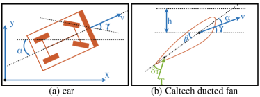
Figure 2: Schematic View of the Case-Study I (a) and II (b)

TABLE I: Results for Case-study I

$\#$Cars	K	$\#$Itr.	Wit. Gen. T.	Fals. T.	Total T.
1	8	2	3	59	66
	10	10	22	40	65
2	32	13	115	98	233
	36	33	423	55	492
3	72	16	274	364	680
	78	44	1903	141	2084
4	128	47	1360	257	1697
	136	62	6766	187	7087

$K$ is the number of model parameters. $\#$Itr. is the number of iterations. Total T. is the total computation time in seconds on a Mac Book Pro with up to 4 GHz Intel Core i7 processor.

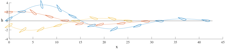
Figure 3: Three execution traces of Case-Study II for the learned policy. $h$ is the height and $x$ is the horizontal position (initially, $x=0$). The wings demonstrate the value of $\beta$ for some time instances. Initial state are as follows. blue:[1 0.5 0.5 0.5 0.5]^t, red:[0 0 0 0 2]^t, and yellow:[-1 -0.5 0.5 0.5 -1]^t.

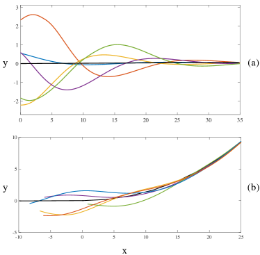
Figure 4: Simulation Results in Webots for Two Road Segments: (a) a straight road, and (b) a curved road. The center of the road is shown with a black line and traces are shown with colored lines starting from different states.

Case-Study II (Caltech Ducted Fan):

We consider an example from Jadbabaie et al. [8], where authors develop a mathematical model for the Caltech ducted fan. The state $\mathbf{x}^{t}=[v\ \gamma\ \beta\ \accentset{\mbox{\large.}}{\beta}\ h]$, consists of speed $v$, angle of velocity $\gamma$, angle of the ducted fan $\beta$, angular velocity $\accentset{\mbox{\large.}}{\beta}$, and height $h$. Fig. 2(b) shows a schematic view of the ducted fan.

The problem here is to stabilize the wing to move forward. The dynamics are:

$$m\accentset{\mbox{\large.}}{v}= -D(v,\alpha)-W\sin(\gamma)+u\cos(\alpha+\delta_{u})$$

$$mv\accentset{\mbox{\large.}}{\gamma}= L(v,\alpha)-W\cos(\gamma)+u\sin(\alpha+\delta_{u})$$

$$J\accentset{\mbox{\large..}}{\beta}= M(v,\alpha)-ul_{T}\sin(\delta_{u})$$

$$\accentset{\mbox{\large.}}{h}= v\sin(\gamma)\,,$$

where $\alpha=\beta-\gamma$, $u$ is the thrust force, and $\delta_{u}$ in the angle for direction of the thrust ($\mathbf{u}^{t}=[u\ \delta_{u}]$) (Cf. [8] for a full description).

The model has a steady state $\mathbf{x}^{*t}=[v_{0}\ 0\ \beta_{0}\ 0\ 0]$, where $v_{0}=6$ and $\beta_{0}=0.177$ (for input $\mathbf{u}^{*t}=[3.2\ -0.138]$), for which the ducted fan steadily moves forward. The fact that dynamics are not affine in control is problematic as we need each $U_{j}$ to be a polyhedron. To get around this, we use $u_{s}:u\ {\sin}(\delta_{u})$ and $u_{c}:u\ {\cos}(\delta_{u})$ as our inputs, and rewrite the equations. The dynamics of the new system are affine in control and $U_{j}$ would be a polyhedron. By setting $\mathbf{x}^{*}$ and $\mathbf{u}^{*}$ as the origins and scaling down $v$, by $2.5$ times

$$\mathbf{x}:=[0.4\ 1\ 1\ 1\ 1]^{t}\circ(\mathbf{x}-\mathbf{x}^{*})\ ,\ \mathbf{u}:=\mathbf{u}-\mathbf{u}^{*}\,,$$

the goal is to reach $G:[-0.2,0.2]^{5}$ from $I:[-0.5,0.5]^{5}$. For the MPC, we use $Q^{\prime}:[0.02\ 0.02\ 1\ 1\ 1\ 1\ 1]$, $H^{\prime}:[15\ 15\ 15\ 15\ 15]$, $\delta=0.3$, $N=15$. Let $\mathcal{T}:\{\tau_{1}(\mathbf{x}),...,\tau_{K^{\prime}}(\mathbf{x})\}$ be set of terms defined over $\mathbf{x}$. Basis functions $v_{k}(\mathbf{x}):\ \mathcal{T}^{\alpha_{k}}$ ($\mathbf{\pi}_{\mathbf{\theta}}:\sum_{k}\mathbf{\theta}_{k}\ \mathcal{T}^{\alpha_{k}}$) correspond to monomials of terms in $\mathcal{T}$, wherein $\alpha_{k}\in\mathbb{N}^{K^{\prime}}$ is a vector of natural number powers such that $|\alpha_{k}|_{1}\leq d$ for some degree bound $d>0$. Both inputs are parameterized with terms $\mathcal{T}:\{v,\gamma,\beta,\accentset{\mbox{\large.}}{\beta},h,\sin(\beta),\cos(\beta)\}$ and degree $d$ is $2$. Using the formal learning algorithm with $\lambda=0.1$, proper parameters are found with $46$ demonstrations. Several traces of $\Psi(\mathcal{F},\mathbf{\pi})$ for the learned policy $\mathbf{\pi}$ is shown in Fig. 3.

The results suggest that our framework can efficiently yield reliable solution to reachability problems, given appropriate basis. Nevertheless, if the bases are not rich enough, the method declares failure after few iterations. For example, when $\mathcal{T}:\{v,\gamma,\beta,\accentset{\mbox{\large.}}{\beta},h\}$, the method terminates in $20$ iterations without any solution.

Comparison with Linear Regression:

We consider a simple supervised learning algorithm in which the demonstrator generates optimal input $\mathbf{u}_{i}$ for a given state $\mathbf{x}_{i}$. Using the demonstrator we generate optimal traces starting from $M$ random initial states. Then, the states in the optimal traces (and their corresponding inputs) are added to the training data. Having a dataset $\{(\mathbf{x}_{1},\mathbf{u}_{1}),\ldots,(\mathbf{x}_{j},\mathbf{u}_{j})\}$, one wishes to find a policy with low error (at least) on the training dataset. In a typical statistical learning procedure, one would minimize the error between the policy and demonstrations:

$$\min_{\theta}\sum_{i=1}^{j}(\pi_{\theta}(\mathbf{x}_{i})-\mathbf{u}_{i})^{2}\,.$$

For both case studies, we tried this statistical learning approach with different training data sizes: $10<M<1000$. In all experiments the falsifier found a trace where the learned policy fails. We believe this notion of error used in regression is merely a heuristic and may not be relevant. For example, we noticed that because of input saturation, many states in the training data have exactly the same corresponding control inputs in the dataset and this prevents a simple linear regression to succeed.

VI Conclusion

We have presented a policy learning approach that combines learning from demonstrations with formal verification, and demonstrated its effectiveness on two case studies. We showed cases where naive supervised learning fails due to its simplicity, whereas our method can solve the problem. Our future work will consider nonlinear models such as deep neural networks as well as extensions to support a richer set of properties beyond reachability.

References

- [1] Alessandro Abate, Iury Bessa, Dario Cattaruzza, Lucas Cordeiro, Cristina David, Pascal Kesseli, and Daniel Kroening. Sound and automated synthesis of digital stabilizing controllers for continuous plants. In Proceedings of the 20th International Conference on Hybrid Systems: Computation and Control, pages 197–206. ACM, 2017.
- [2] Brenna D Argall, Sonia Chernova, Manuela Veloso, and Brett Browning. A survey of robot learning from demonstration. Robotics and autonomous systems, 57(5):469–483, 2009.
- [3] L El Ghaoui and V Balakrishnan. Synthesis of fixed-structure controllers via numerical optimization. In Decision and Control, 1994., Proceedings of the 33rd IEEE Conference on, volume 3, pages 2678–2683. IEEE, 1994.
- [4] Xiaoxiao Guo, Satinder Singh, Honglak Lee, Richard L Lewis, and Xiaoshi Wang. Deep learning for real-time atari game play using offline monte-carlo tree search planning. In Advances in neural information processing systems, pages 3338–3346, 2014.
- [5] He He, Jason Eisner, and Hal Daume. Imitation learning by coaching. In Advances in Neural Information Processing Systems, pages 3149–3157, 2012.
- [6] Zhenqi Huang, Yu Wang, Sayan Mitra, Geir E Dullerud, and Swarat Chaudhuri. Controller synthesis with inductive proofs for piecewise linear systems: An smt-based algorithm. In 2015 54th IEEE Conference on Decision and Control (CDC), pages 7434–7439. IEEE, 2015.
- [7] A. Jadbabaie and J. Hauser. On the stability of receding horizon control with a general terminal cost. IEEE Transactions on Automatic Control, 50(5):674–678, 2005.
- [8] Ali Jadbabaie and John Hauser. Control of a thrust-vectored flying wing: a receding horizon-lpv approach. International Journal of Robust and Nonlinear Control, 12(9):869–896, 2002.
- [9] Susmit Jha, Sumit Gulwani, Sanjit A. Seshia, and Ashish Tiwari. Synthesizing switching logic for safety and dwell-time requirements. In Proceedings of the International Conference on Cyber-Physical Systems (ICCPS), pages 22–31, April 2010.
- [10] Susmit Jha and Sanjit A Seshia. A theory of formal synthesis via inductive learning. Acta Informatica, pages 1–34, 2017.
- [11] Gregory Kahn, Tianhao Zhang, Sergey Levine, and Pieter Abbeel. Plato: Policy learning using adaptive trajectory optimization. In Robotics and Automation (ICRA), 2017 IEEE International Conference on, pages 3342–3349. IEEE, 2017.
- [12] Seyed Mohammad Khansari-Zadeh and Oussama Khatib. Learning potential functions from human demonstrations with encapsulated dynamic and compliant behaviors. Autonomous Robots, 41(1):45–69, 2017.
- [13] Ron Koymans. Specifying real-time properties with metric temporal logic. Real-time systems, 2(4):255–299, 1990.
- [14] Sergey Levine and Vladlen Koltun. Learning complex neural network policies with trajectory optimization. In International Conference on Machine Learning, pages 829–837, 2014.
- [15] Weiwei Li and Emanuel Todorov. Iterative linear quadratic regulator design for nonlinear biological movement systems. In ICINCO (1), pages 222–229, 2004.
- [16] Jun Liu, Necmiye Ozay, Ufuk Topcu, and Richard M Murray. Synthesis of reactive switching protocols from temporal logic specifications. Automatic Control, IEEE Transactions on, 58(7):1771–1785, 2013.
- [17] D.Q. Mayne, J.B. Rawlings, C.V. Rao, and P.O.M. Scokaert. Constrained model predictive control: Stability and optimality. Automatica, 36(6):789 – 814, 2000.
- [18] Manuel Mazo, Anna Davitian, and Paulo Tabuada. Pessoa: A tool for embedded controller synthesis. In International Conference on Computer Aided Verification, pages 566–569. Springer, 2010.
- [19] Olivier Michel. Cyberbotics Ltd. Webots: Professional mobile robot simulation. International Journal of Advanced Robotic Systems, 1(1):5, 2004.
- [20] Igor Mordatch and Emo Todorov. Combining the benefits of function approximation and trajectory optimization. In Robotics: Science and Systems, pages 5–32, 2014.
- [21] Necmiye Ozay, Jun Liu, Priyanka Prabhakar, and Richard M Murray. Computing augmented finite transition systems to synthesize switching protocols for polynomial switched systems. In American Control Conference (ACC), 2013, pages 6237–6244. IEEE, 2013.
- [22] Vasumathi Raman, Alexandre Donzé, Dorsa Sadigh, Richard M Murray, and Sanjit A Seshia. Reactive synthesis from signal temporal logic specifications. In Proc. HSCC’15, pages 239–248. ACM, 2015.
- [23] Hadi Ravanbakhsh and Sriram Sankaranarayanan. Infinite horizon safety controller synthesis through disjunctive polyhedral abstract interpretation. In Embedded Software (EMSOFT), 2014 International Conference on, pages 1–10. IEEE, 2014.
- [24] Hadi Ravanbakhsh and Sriram Sankaranarayanan. Counter-example guided synthesis of control lyapunov functions for switched systems. In 2015 54th IEEE Conference on Decision and Control (CDC), pages 4232–4239. IEEE, 2015.
- [25] Hadi Ravanbakhsh and Sriram Sankaranarayanan. Learning control lyapunov functions from counterexamples and demonstrations. Autonomous Robots, pages 1–33, 8 2018.
- [26] Stéphane Ross, Geoffrey J Gordon, and Drew Bagnell. A reduction of imitation learning and structured prediction to no-regret online learning. In International Conference on Artificial Intelligence and Statistics, pages 627–635, 2011.
- [27] Matthias Rungger and Majid Zamani. Scots: A tool for the synthesis of symbolic controllers. In Proceedings of the 19th International Conference on Hybrid Systems: Computation and Control, pages 99–104. ACM, 2016.
- [28] Armando Solar-Lezama, Liviu Tancau, Rastislav Bodik, Sanjit Seshia, and Vijay Saraswat. Combinatorial sketching for finite programs. ACM SIGOPS Operating Systems Review, 40(5):404–415, 2006.
- [29] Ankur Taly, Sumit Gulwani, and Ashish Tiwari. Synthesizing switching logic using constraint solving. International journal on software tools for technology transfer, 13(6):519–535, 2011.
- [30] Weehong Tan and Andrew Packard. Searching for control lyapunov functions using sums of squares programming. sibi, 1:1, 2004.
- [31] Lieven Vandenberghe, Stephen Boyd, and Shao-Po Wu. Determinant maximization with linear matrix inequality constraints. SIAM journal on matrix analysis and applications, 19(2):499–533, 1998.
- [32] Marcell Vazquez-Chanlatte, Shromona Ghosh, Vasumathi Raman, Alberto Sangiovanni-Vincentelli, and Sanjit A. Seshia. Generating dominant strategies for continuous two-player zero-sum games. In IFAC Conference on Analysis and Design of Hybrid Systems (ADHS), 2018.
- [33] Boyan Yordanov and Calin Belta. Parameter synthesis for piecewise affine systems from temporal logic specifications. In International Workshop on Hybrid Systems: Computation and Control, pages 542–555. Springer, 2008.
- [34] Mingyuan Zhong, Mikala Johnson, Yuval Tassa, Tom Erez, and Emanuel Todorov. Value function approximation and model predictive control. In 2013 IEEE Symposium on Adaptive Dynamic Programming and Reinforcement Learning (ADPRL), pages 100–107. IEEE, 2013.