PuVAE: A Variational Autoencoder to Purify Adversarial Examples

Abstract

Deep neural networks are widely used and exhibit excellent performance in many areas. However, they are vulnerable to adversarial attacks that compromise the network at the inference time by applying elaborately designed perturbation to input data. Although several defense methods have been proposed to address specific attacks, other attack methods can circumvent these defense mechanisms. Therefore, we propose Purifying Variational Autoencoder (PuVAE), a method to purify adversarial examples. The proposed method eliminates an adversarial perturbation by projecting an adversarial example on the manifold of each class, and determines the closest projection as a purified sample. We experimentally illustrate the robustness of PuVAE against various attack methods without any prior knowledge. In our experiments, the proposed method exhibits performances competitive with state-of-the-art defense methods, and the inference time is approximately 130 times faster than that of Defense-GAN that is the state-of-the art purifier model.

1 Introduction

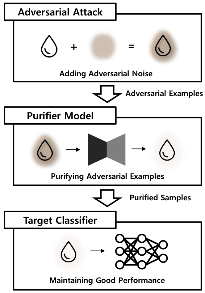
Figure 1: Overview of the defense mechanism using the purifier model.

Significant progress has characterized deep learning in several areas including image recognition He et al. (2016), disease prediction Hwang et al. (2017), and autonomous driving Yoo et al. (2017). However, security issues of deep neural networks, which are especially vulnerable to adversarial attacks, are emerging. The goal of adversarial attacks is to fool deep neural networks via applying elaborately designed perturbation to input data. Adversarial attacks make it hazardous to apply deep neural networks in real world applications. In the case of autonomous driving Akhtar and Mian (2018), attacks can cause an accident by making an object detector recognize pedestrians as roads.

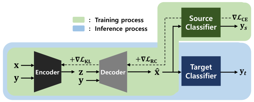
Figure 2: Overview of the PuVAE algorithm; The green region represents the training process, and the blue region denotes the inference process of PuVAE. The dotted line is the gradient flow in training process. The parameters of the source classifier are not updated.

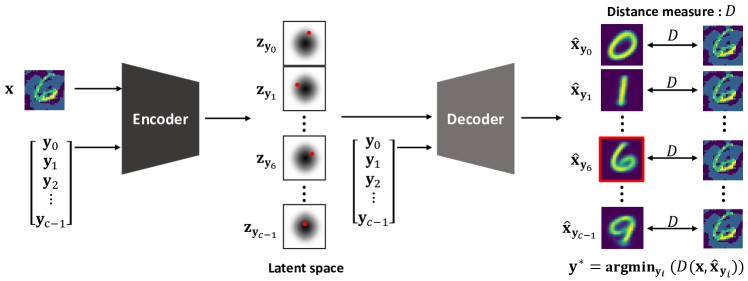
Figure 3: Inference of PuVAE with an MNIST image; A latent vector $\mathbf{z}_{\mathbf{y}_{i}}$ is sampled from an adversarial sample $\mathbf{x}$ and a class condition $\mathbf{y}_{i}$.

To address these attacks, several defense mechanisms have been proposed. There are three categories of defense mechanisms. The first mechanisms involve modifying the training dataset such that the classifier is robust against the adversarial attack Szegedy et al. (2013). Second mechanisms block gradient calculation via changing the training procedure Buckman et al. (2018); Guo et al. (2017). However, they are only effective for the gradient based attack methods. The third mechanisms involve removing the adversarial noise from the sample fed into the classifier Samangouei et al. (2018).

Our main focus is defense mechanisms to purify input data that may have added adversarial perturbation; this can allow the mechanisms to effectively address any attacks. These methods mostly work by using a generative model to learn the data distribution and project the adversarial example into the learned data distribution $p(x)$. We term the generative models as purifiers, and MagNet Meng and Chen (2017) and Defense-GAN Samangouei et al. (2018) are recent work. In Figure 1, we show an overview of the defense mechanism using the purifier model.

Specifically, MagNet learns the original data using one or more autoencoders termed as the reformer networks and passes input data to the autoencoders that move input data closer to the data manifold. The purified data are supplied to the classifier. However, the method has a disadvantage wherein it exhibits poor performance when compared with Defense-GAN.

Defense-GAN uses the characteristics of generative adversarial networks (GANs) to defend a target model against adversarial attacks. It uses the fact that optimizing the objective function of the GAN is equivalent to making the generator distribution $p_{g}$ identical to the data distribution $p_{data}$. After training the GAN using the original data, Defense-GAN iteratively finds generator input $z$ through the gradients. This reduces the reconstruction error between the generated data $G(z)$ and the input data $x$ that may have added adversarial noise. Subsequently, data generated with optimal $z$ are supplied to the classifier as input. The model relies on the unstable performance of GAN, and this occationally reproduces adversarial noise by directly optimizing errors between the adversarial example $x+\delta$ and the generated sample $G(z)$. In addition, because of Defense-GAN’s iterative nature, it takes a long time to yield the maximum defense performance. In particular, real-time applications such as object detection must operate in a short period of time, so a fast defense algorithm needs to be developed.

In this paper, we aim to rapidly generate well-classified samples from adversarial examples. The purified samples are fed into the target classifier so that they are classified without being affected by adversarial attacks. To solve the limitations of MagNet and Defense-GAN, we propose Purifying Variational AutoEncoder (PuVAE) that purifies adversarial examples using a Variational Autoencoder (VAE). The proposed model uses variational inference to generate samples that provide comparable or better defense performance than the state-of-the-art model. In contrast to Defense-GAN, PuVAE generates clean samples with one feed-forward step. Therefore, our method is robust against adversarial attacks within a reasonable time limit.

In summary, our contributions are as follows:

• We propose a VAE-based defense method, PuVAE, to effectively purify adversarial attacks. The proposed method shows a remarkable performanc over other defense methods.

• The proposed method significantly reduces the time to generate purified samples. Within a reasonable time limit, PuVAE outperforms state-of-the-art defense methods.

• Experimental results demonstrate that our method functions robustly against a variety of attack methods and datasets.

2 Background

2.1 Variational Autoencoder (VAE)

A generative model is used to represent data distribution. Most data are too complex to directly find the relation in themselves, and thus relatively simple latent variables are typically used to represent data distribution. Kingma Kingma and Welling (2013) introduced Variational AutoEncoder (VAE), which is a method that uses a combination of neural networks and variational inference to learn a decoder that generates data from normal distribution. The objective function of VAE is represented as follows:

$$\log(p(x))=D_{KL}(q_{\phi}(z|x)||p_{\theta}(z|x))+\mathcal{L}(\theta,\phi,x)$$ (1)

$$\mathcal{L}(\theta,\phi,x)=-D_{KL}(q_{\phi}(z |x)||p_{\theta}(z))$$

$$+E_{z\sim q_{\phi}(z|x)}[\log(p_{\theta}(x|z))]$$ (2)

where $log(p(x))$ denotes the marginal log likelihood of the data, $\mathcal{L}(\theta,\phi,x)$ denotes the variational lower bound of marginal likelihood, $p_{\theta}(x|z)$ denotes the output distribution of the decoder, $q_{\phi}(z|x)$ denotes the output distribution of the encoder, and $p_{\theta}(z)$ denotes a normal distribution. By maximizing the lower bound, marginal likelihood of data is maximized. In VAE, latent space is assumed as a multivariate Gaussian distribution.

Doersch Doersch (2016) indicated that conditional Variational Autoencoder (cVAE) is specifically used to learn a multimodal distribution via class information. The basic idea of cVAE is similar to that of VAE, which aims to learn the distribution of data. However, the encoder and the decoder of cVAE take a class label as an additional input.

In this study, we select a cVAE structure to learn class-specific data distributions. We use the encoder as the mapping function of adversarial examples to the latent space of legitimate images and the decoder as the reconstructor of images from the latent spaces. We confirm that the forwarding process via the encoder-decoder model effectively purifies adversarial noise from data.

2.2 Adversarial Examples

An adversarial example is a sample that is designed to be misclassified by the target classifier by using intended noise that is not perceivable by humans. Prior to a study by Goodfellow Goodfellow et al. (2015), attackers exploited the non-linearity of neural networks. However, the authors claimed that the cause of vulnerability to adversarial examples is a linear characteristic of neural networks and proposed the Fast Gradient Sign Method (FGSM) that uses the gradient from the objective function of neural networks.

Although FGSM is a fast algorithm to make adversarial attacks, it is easy to defend the one step gradient based approach. In order to overcome the problem, the iterative Fast Graident Sign Method (iFGSM) was proposed by Kurakin Kurakin et al. (2016). The method optimizes adversarial noise in several steps with a small perturbation of an image which allows a more accurate attack.

RAND+FGSM Tra (2017) is a new attack method that adds random Gaussian noise to an image, and computes FGSM with the perturbed image. Against the FGSM-based methods, we used targeted adversarial attacks because we assume that it is more difficult to defend targeted attacks than untargeted attacks Xu et al. (2019). In our experiment, we randomly chose target labels among classes with the exception of the true class.

The Carlini and Wagner (CW) attack suggested by Carlini Car (2017) is the most powerful attack method among existing methods. By solving the optimization problem in a gradient descent manner, adversarial perturbation is derived as follows:

$$\mathrm{minimize}~{}~{} ||\delta||_{p}+c*f(x+\delta)$$ (3)

$$\mathrm{subject~{}to}~{}~{} x+\delta\in[0,1]^{n}$$ (4)

where $f(x)$ denotes an objective function of a classifier and $\delta$ denotes perturbation added to image $x$. In this study, we used $p=2$ and created CW attack with open source software CleverHans by Papernot Papernot et al. (2018) to verify whether our method can defend the attack.

3 Proposed Method

In this paper, we propose a VAE-based defense method that is coined as PuVAE to purify adversarial noise from data. We consider a dataset $\mathcal{X}_{\mathrm{data}}$ that consists of data instances $\mathbf{x}_{\mathrm{data}}\in\mathbb{R}^{d}$ where $d$ denotes the dimension of the data space. Corresponding class labels (one-hot vectors) are denoted by $\mathbf{y}_{\mathrm{data}}\in\mathbb{R}^{c}$ in a set of classes $C$ where $c$ is the number of classes.

We then consider a target classifier $M_{t}$ that is the model an attacker wants to attack. We also assume a set $\mathcal{X}_{\mathrm{adv}}$ that consists of adversarial examples $\mathbf{x}_{\mathrm{adv}}\in\mathbb{R}^{d}$ created from the target classifier. We define a set $\mathcal{X}$ which contains clean samples and adversarial examples. Instances $\mathbf{x}$ from the set $\mathcal{X}$ are used at inference time. We explain the procedures of training and generating purified samples using PuVAE. The overview of the proposed method is described in Figure 2.

3.1 Training process of PuVAE

PuVAE is comprised of an encoder and a decoder network. The encoder receives a data-label pair and outputs the mean $\boldsymbol{\mu}$ and the standard deviation $\boldsymbol{\sigma}$ of the Gaussian distribution on the latent space corresponding to the input label:

$$\boldsymbol{\mu},\boldsymbol{\sigma} =\mathrm{Encoder}(\mathbf{x}_{\mathrm{data}},\mathbf{y}_{\mathrm{data}})$$ (5)

Using $\mathbf{\mu}$ and $\mathbf{\sigma}$ obtained from the encoder, the latent vector $\mathbf{z}$ on the latent space is sampled:

$$\mathbf{z} =\boldsymbol{\mu}+\boldsymbol{\epsilon}\cdot\boldsymbol{\sigma}$$ (6)

$$\boldsymbol{\epsilon} \sim N(\mathbf{0},\sigma_{\epsilon}\mathbf{I})$$ (7)

where $\boldsymbol{\epsilon}$ denotes a random variable for the reparameterization trick, and $\sigma_{\epsilon}$ denotes a hyperparameter that is multiplied by the standard deviation to control the extent to which the latent vector is sampled. In the experiments, we used $\sigma_{\epsilon}=1$ in the training time to ensure that the posterior latent distribution follows the normal distribution.

In classification tasks, Convolutional Neural Networks (CNNs) using pooling and strides are used to select useful features and to widen receptive field. However, this selective nature of CNNs is a disadvantage on generative models, since the feature selection causes information loss. Therefore, we use a dilated convolutional neural network as the encoder to get the latent vector $\mathbf{z}$. Dilated convolution inserts zeros in the filter, so that the receptive field is enlarged and information loss is effectively reduced.

the sampled $\mathbf{z}$ enters the decoder with the label and produces an output instance $\hat{\mathbf{x}}$ with the same dimension $d$ as the input:

$$\hat{\mathbf{x}}=\mathrm{Decoder}(\mathbf{z},\mathbf{y}_{\mathrm{data}})$$ (8)

At the training time, PuVAE is trained to maximize the variational lower bound in a manner similar to cVAE. Loss functions from the encoder and the decoder are:

$$\mathcal{L}_{\mathrm{RC}}= ~{}\mathbf{x}_{\mathrm{data}}\log\hat{\mathbf{x}}+(1-\mathbf{x}_{\mathrm{data}})\log(1-\hat{\mathbf{x}})$$ (9)

$$\mathcal{L}_{\mathrm{KL}}=\boldsymbol{\mu}^{2}+\boldsymbol{\sigma}^{2}-\log(\boldsymbol{\sigma}^{2}-1)$$ (10)

where $\mathcal{L}_{\mathrm{RC}}$ denotes the reconstruction loss function to minimize the difference between the input instance and output instance, and $\mathcal{L}_{\mathrm{KL}}$ denotes Kullback-Leibler divergence between the output distribution of the encoder and the normal distribution. This process allows PuVAE to construct the mapping of legitimate data on the latent space

Additionally, we use the cross-entropy calculated from a classifier as a loss function for PuVAE. The classifier, called source classifier $M_{s}$, learns the decision boundaries on the data space. Since neural networks performing the same task learn similar functions Goodfellow et al. (2015), we use a fixed architecture for $M_{s}$. Then, trained $M_{s}$ is used to ensure that the output instance reflects the characteristic of the classes in $C$. The cross-entropy loss from $M_{s}$ is as follows:

$$\mathbf{y}_{s} =M_{s}(\hat{\mathbf{x}})$$ (11)

$$\mathcal{L}_{\mathrm{CE}}=\mathbf{y}_{\mathrm{data}}\log\mathbf{y}_{s} +(1-\mathbf{y}_{\mathrm{data}})\log(1-\mathbf{y}_{s})$$ (12)

Finally, PuVAE is trained using the stochastic gradient descent (SGD):

$$\nabla({\lambda}_{\mathrm{RC}}\mathcal{L}_{\mathrm{RC}}+{\lambda}_{\mathrm{KL}}\mathcal{L}_{\mathrm{KL}}+{\lambda}_{\mathrm{CE}}\mathcal{L}_{\mathrm{CE}})$$ (13)

where ${\lambda}_{\mathrm{KL}}$, ${\lambda}_{\mathrm{RC}}$, ${\lambda}_{\mathrm{CE}}$ are coefficients for each loss functions.

Table 1: Neural network architectures for PuVAE.

Encoder	Decoder
Dilated Conv(32, 7$\times$7, 2)	FC(512)
ReLU	ReLU
Dilated Conv(32, 7$\times$7, 2)	Deconv(32, 7$\times$7, 2)
ReLU	ReLU
Dilated Conv(32, 7$\times$7, 2)	Deconv(32, 7$\times$7, 2)
ReLU	ReLU
FC(1024)	Deconv(32, 7$\times$7, 2)
ReLU	Sigmoid
FC(1024)
ReLU
FC(64)
Softplus (for $\sigma$ only)

3.2 Generating Purified Samples

At the inference time, PuVAE projects an input sample to the data manifolds of all classes in $C$ as follows:

$$\hat{\mathbf{x}}_{\mathbf{y}_{i}}=\mathrm{PuVAE}(\mathbf{x},\mathbf{y}_{i})$$ (14)

where $\mathbf{y}_{i}$ denotes the $i$-th class label in $C$ to guide the input to the corresponding latent space, and $\hat{\mathbf{x}}_{\mathbf{y}_{i}}$ denotes a candidate for the purified sample. The inference also follows the Equations (5), (6), and (7) as in training, where $\sigma_{\epsilon}$ is used to sample the latent vector $\mathbf{z}$. We performed a hyperparameter search on $\sigma_{\epsilon}$ among $\{0,0.01,0.1,1,10,100\}$ for the inference. Thus, the optimal value of $\sigma_{\epsilon}$ is 0.1.

Because PuVAE only learns the distribution of $\mathbf{z}$ from the training data, the input data is mapped to the learned latent spaces even if adversarial example comes in. the adversarial noise is removed in the projection to the latent variable.

Then, the class label corresponding to the closest projection, $\mathbf{y}^{*}$, is selected as follows:

$$\mathbf{y}^{*}=\operatorname{\mathrm{argmin}}_{\mathbf{y}_{i}\in C}~{}{D(\mathbf{x},\hat{\mathbf{x}}_{\mathbf{y}_{i}})}$$ (15)

where $D$ denotes a distance measure to determine the closest projection. We use the root mean square error (RMSE) as the distance measure. Therefore, the candidate generated with label $\mathbf{y}^{*}$ is the purified sample which goes into $M_{t}$:

$$\mathbf{x}_{\mathrm{purified}}=\hat{\mathbf{x}}_{\mathbf{y}^{*}}$$ (16)

Finally, the purified sample is fed into the target classifier $M_{t}$ as follows:

$$\mathbf{y}_{t}=M_{t}(\mathbf{x}_{\mathrm{purified}})$$ (17)

The complete process of generating the purified sample using PuVAE is illustrated in Figure 3.

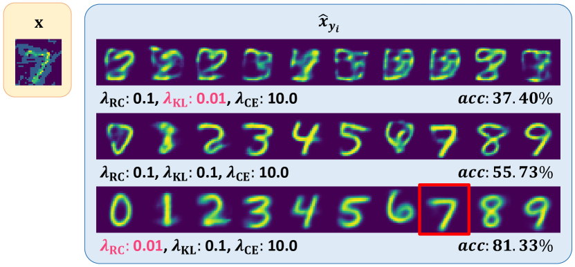
Figure 4: Comparison of coefficients for training PuVAE; an adversarial example is highlighted with the yellow box The blue box represents the output samples when the input $\mathbf{x}$ enters. Each row shows output images from the model trained in different coefficient combinations. Each column shows images sequentially conditioned on class labels $0\sim 9$. $acc$ denotes the defense performance from $M_{t}$ using the coefficient combination of each row.

4 Experiments

Table 2: Defense performance on the MNIST dataset (%).

Classifier	Attacks	No Attack	No Defense	Adv. Tr.	MagNet	Defense-GAN	PuVAE
A	FGSM (0.3)	99.51	12.46	78.57	26.90	85.29	81.33
	iFGSM (0.3)	99.51	0.00	91.72	72.48	87.40	92.33
	RAND+FGSM (0.05, 0.3)	99.51	10.64	84.21	32.34	89.02	82.70
	CW (100)	99.51	0.43	18.80	18.80	90.04	90.80
B	FGSM (0.3)	99.29	28.85	88.49	71.70	86.03	88.25
	iFGSM (0.3)	99.29	0.04	93.56	86.29	88.55	92.25
	RAND+FGSM (0.05, 0.3)	99.29	6.42	88.44	41.66	89.76	85.03
	CW (100)	99.29	0.59	19.20	19.10	90.76	92.92

Table 3: Defense performance on the Fashion-MNIST dataset (%).

Classifier	Attacks	No Attack	No Defense	Adv. Tr.	MagNet	Defense-GAN	PuVAE
A	FGSM (0.3)	93.46	4.06	11.51	11.71	56.67	59.18
	iFGSM (0.3)	93.46	0.00	50.31	34.70	65.11	72.51
	RAND+FGSM (0.05, 0.3)	93.46	1.60	8.72	6.96	59.52	45.13
	CW (100)	93.46	5.01	18.00	15.50	68.60	80.59
B	FGSM (0.3)	93.54	2.75	8.00	15.30	58.20	52.46
	iFGSM (0.3)	93.54	0.00	46.97	41.84	66.06	71.04
	RAND+FGSM (0.05, 0.3)	93.54	1.34	9.93	7.44	60.98	52.22
	CW (100)	93.54	4.87	16.70	16.70	67.62	79.42

Table 4: Defense performance on the CIFAR-10 dataset (%).

Classifier	Attacks	No Attack	No Defense	Adv. Tr.	MagNet	Defense-GAN	PuVAE
C	FGSM (0.06)	82.13	3.82	19.07	18.58	29.74	33.71
	iFGSM (0.06)	82.13	0.32	24.13	27.00	33.69	35.49
	RAND+FGSM (0.005, 0.06)	82.13	4.84	21.27	19.99	36.74	33.76
	CW (100)	82.13	9.88	56.48	40.13	38.13	36.36
D	FGSM (0.06)	80.30	3.19	15.00	18.98	30.11	33.20
	iFGSM (0.06)	80.30	0.43	21.51	29.95	32.47	34.48
	RAND+FGSM (0.005, 0.06)	80.30	4.13	18.55	20.44	35.76	34.40
	CW (100)	80.30	9.92	13.64	15.71	28.10	31.70

In this section, we determine optimal setting for PuVAE, and present the defense performance of PuVAE against adversarial attacks. We used Tensorflow (1.12.0) for the experiments. A GPU, an NVIDIA TITAN V (12 GB), and a CPU, an Intel Xeon E5-2690 v4 (2.6 GHz), were used. We used MNIST LeCun et al. (1998) which is a hand-written digit dataset, Fashion-MNIST Xiao et al. (2017) which is a clothing object image dataset, and CIFAR-10 Krizhevsky and Hinton (2009) which is a tiny natural image dataset. Each dataset consists of 50,000 training instances and 10,000 test instances. We normalized data between 0 and 1.

We used FGSM, iFGSM, RAND+FGSM, and CW attacks for the experiments. FGSM, iFGSM, and RAND+FGSM were generated with an adversarial perturbation size of 0.3 for the MNIST and Fashion-MNIST datasets, and 0.06 for the CIFAR-10 dataset. We set the upper limit on the random noise of RAND+FGSM as 0.05 for the MNIST and the Fashion-MNIST datasets, and 0.005 for the CIFAR-10 dataset. We set the number of iterations of the CW attack as 100 on all datasets. The performance of defense mechanisms is measured by the accuracy of the target classifier.

The architectures of the encoder and the decoder of PuVAE are presented in Table 1. Dilated Conv($n$, $k\times k$, $r$) denotes a dilated convolution layer with $n$ feature maps, filter size $k\times k$, and dilation rate $r$. Deconv($n$, $k\times k$, $s$) denotes a deconvolution layer with $n$ feature maps, filter size $k\times k$, and stride $s$. FC($m$) denotes a fully connected layer with $m$ units. ReLU denotes the rectified linear unit. We use the first half of the last layer of the encoder, 32 output units, as $\mu$ and the second half is passed to the softplus function to infer $\sigma$. We used the architecture of Defense-GAN and the reformer network of MagNet as suggested in Samangouei et al. (2018) and Meng and Chen (2017) respectively. The architectures of $M_{t}$ and $M_{s}$ are shown in the Supplementary Materials.

4.1 Effect of coefficients on Training PuVAE

Figure 4 demonstrates the characteristics of generated samples based on the combinations of three coefficients $\lambda_{\mathrm{RC}}$, $\lambda_{\mathrm{KL}}$, and $\lambda_{\mathrm{CE}}$. If $\lambda_{\mathrm{RC}}$ is larger than $\lambda_{\mathrm{KL}}$, the constraint of the posterior distribution of the encoder is relieved. Thus, the encoder easily maps the input samples to the low likelihood area of the latent space. The characteristic of this mapping causes the decoder to generate strange image as demonstrated in the first row of Figure 4.

Conversely, the typical form of each class is generated when $\lambda_{\mathrm{KL}}$ is large in model learning. Therefore, as shown in the last row of Figure 4, it is possible to generate samples that exhibit distinctive characteristics of each class even if an input sample in other classes come in. The red box of Figure 4 illustrate that the purified sample $\mathbf{x}_{\mathrm{purified}}$ is analogous to the input sample $\mathbf{x}$, with the effect of adversarial noise removed. Additionally, the highest defense performance is acquired from the coefficient combination in the last row of Figure 4. Therefore, we set $\lambda_{\mathrm{RC}}$, $\lambda_{\mathrm{KL}}$ and $\lambda_{\mathrm{CE}}$ to 0.01, 0.1, and 10, respectively, as coefficients in experiments.

4.2 Defense Performance

In this section, we compare the defense performance of PuVAE with maximum defense abilities of adversarial training, MagNet, and Defense-GAN. To obtain the best performance of Defense-GAN, we set the number of iterations as 200 and the number of candidates as 20. Tables 2, 3, and 4 show the performances of defense methods on the MNIST, the Fashion-MNIST, and the CIFAR-10 datasets respectively.

As shown in Table 2, the performance of PuVAE exceeds that of MagNet on all attacks and is comparable to that of Defense-GAN. Adversarial training is also comparable with our method in FGSM, iFGSM, and RAND+FGSM albeit a very low performance in the CW attack. Since we used gradients from $M_{t}$ for adversarial training, it is robust against gradient based attacks (FGSM, iFGSM, and RAND+FGSM), but weak against the other attack.

As shown in Table 3, PuVAE shows the best performance against iFGSM and the CW attacks in both architectures. Even though iFGSM is the most difficult attack when there is no defense, the proposed model effectively defends the attack. The purified images on the MNIST and the Fasion-MNIST datsets are visualized in Supplementary Materials.

As shown in Table 4, the CIFAR-10 dataset shows overall low accuracy. Although adversarial training exhibits the best performance at a certain setting, it shows unstable results depending on models and attacks. However, PuVAE shows the best performance in various attacks and model architectures. Our method also exhibits a robust performance in settings where it does not take the first place. This indicates that the proposed method shows the general defense ability across various attacks.

4.3 Performance in a Reasonable Time Constraint

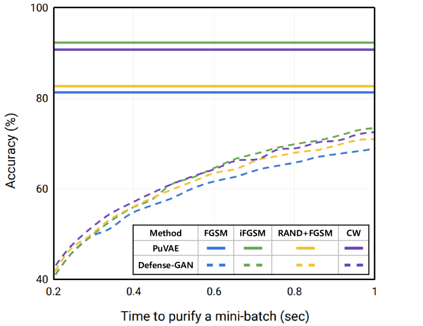
Figure 5: Comparison with Defense-GAN in a reasonable time constraint.

Defense mechanisms including Defense-GAN and PuVAE purify adversarial examples in a pre-processing manner. In contrast to PuVAE, Defense-GAN takes a significant amount of time to derive the maximum performance. While Defense-GAN takes approximately 14.8 seconds, PuVAE takes 0.114 seconds to purify a mini-batch with 128 MNIST images, allowing nearly 130 times faster inference as shown in Table 5.

The security issue of adversarial attacks becomes particularly prominent in autonomous driving because it is not plausible to apply purifying-models that take a considerable amount of time to real-time applications. This setback of Defense-GAN accentuates the need for time-efficient defense methods. Therefore, we measured the performance based on a reasonable time limit with the MNIST dataset. In the experiments, we set the time limit as one second.

In Figure 5, the solid lines show the performances of PuVAE, and the dotted lines show the performances of Defense-GAN. Each color denotes a different attack method. PuVAE performs with one inference, and thus the performance of PuVAE is superior to that of Defense-GAN within the time limit. Since Defense-GAN creates a hidden vector iteratively by the gradient-based optimization process, the performance increases as time lapses. However, its performance does not reach the performance of PuVAE in the time limit. Therefore, PuVAE is more efficient than the state-of-the-art method for real-time applications.

It is unfair to compare PuVAE and Defense-GAN without time constraint because the inference time of Defense-GAN significantly exceeds that of PuVAE. We compared the two defense methods after setting the time limit to one second. As shown in Table 6, it is observed that the performance of Defense-GAN is significantly lower than its maximum performance. Therefore, PuVAE is more practical in real-world scenarios because it exhibits the highest performance in a reasonable time condition.

Table 5: Inference time comparison of PuVAE and Defense-GAN.

Method	PuVAE	Defense-GAN
Time (seconds)	0.11	14.80
Ratio	1	134.55

Table 6: Accuracy of defense methods within one second (%).

Method	FGSM	iFGSM	RAND+FGSM	CW
Adv. Tr.	78.57	91.72	84.21	18.80
MagNet	26.90	72.48	32.34	18.80
Defense-GAN	69.25	73.85	71.50	72.79
PuVAE	81.33	92.33	82.70	90.80

5 Conclusion

In this paper, we propose PuVAE, a novel VAE-based defense method that effectively purifies adversarial attacks. PuVAE is robust against various attacks and overcomes the disadvantages of adversarial training. The performance of PuVAE is also comparable to the best performance of Defense-GAN. In addition, PuVAE significantly ourperforms Defense-GAN given a reasonable time limit. We demonstrate the advantages of the proposed method on various datasets and adversarial attacks. For future work, we plan to apply our method to real-time applications such as autonomous-driving, face identification, and surveillance systems.

References

- Akhtar and Mian [2018] Naveed Akhtar and Ajmal Mian. Threat of adversarial attacks on deep learning in computer vision: A survey. IEEE Access, 6:14410–14430, 2018.
- Buckman et al. [2018] Jacob Buckman, Aurko Roy, Colin Raffel, and Ian Goodfellow. Thermometer encoding: One hot way to resist adversarial examples. In Submissions to International Conference on Learning Representations, 2018.
- Car [2017] Towards evaluating the robustness of neural networks. arXiv preprint arXiv:1608.04644, 2017.
- Doersch [2016] Carl Doersch. Tutorial on variational autoencoders. arXiv preprint arXiv:1606.05908, 2016.
- Goodfellow et al. [2015] Ian Goodfellow, Jonathon Shlens, and Christian Szegedy. Explaining and harnessing adversarial examples. In International Conference on Learning Representations, 2015.
- Guo et al. [2017] Chuan Guo, Mayank Rana, Moustapha Cisse, and Laurens van der Maaten. Countering adversarial images using input transformations. arXiv preprint arXiv:1711.00117, 2017.
- He et al. [2016] Kaiming He, Xiangyu Zhang, Shaoqing Ren, and Jian Sun. Deep residual learning for image recognition. In Proceedings of the IEEE conference on computer vision and pattern recognition, pages 770–778, 2016.
- Hwang et al. [2017] Uiwon Hwang, Sungwoon Choi, and Sungroh Yoon. Disease prediction from electronic health records using generative adversarial networks. arXiv preprint arXiv:1711.04126, 2017.
- Kingma and Welling [2013] Diederik P Kingma and Max Welling. Auto-encoding variational bayes. arXiv preprint arXiv:1312.6114, 2013.
- Krizhevsky and Hinton [2009] Alex Krizhevsky and Geoffrey Hinton. Learning multiple layers of features from tiny images. Technical report, Citeseer, 2009.
- Kurakin et al. [2016] Alexey Kurakin, Ian Goodfellow, and Samy Bengio. Adversarial examples in the physical world. arXiv preprint arXiv:1607.02533, 2016.
- LeCun et al. [1998] Yann LeCun, Léon Bottou, Yoshua Bengio, Patrick Haffner, et al. Gradient-based learning applied to document recognition. Proceedings of the IEEE, 86(11):2278–2324, 1998.
- Meng and Chen [2017] Dongyu Meng and Hao Chen. Magnet: a two-pronged defense against adversarial examples. In Proceedings of the 2017 ACM SIGSAC Conference on Computer and Communications Security, pages 135–147. ACM, 2017.
- Papernot et al. [2018] Nicolas Papernot, Fartash Faghri, Nicholas Carlini, Ian Goodfellow, Reuben Feinman, Alexey Kurakin, Cihang Xie, Yash Sharma, Tom Brown, Aurko Roy, Alexander Matyasko, Vahid Behzadan, Karen Hambardzumyan, Zhishuai Zhang, Yi-Lin Juang, Zhi Li, Ryan Sheatsley, Abhibhav Garg, Jonathan Uesato, Willi Gierke, Yinpeng Dong, David Berthelot, Paul Hendricks, Jonas Rauber, and Rujun Long. Technical report on the cleverhans v2.1.0 adversarial examples library. arXiv preprint arXiv:1610.00768, 2018.
- Samangouei et al. [2018] Pouya Samangouei, Maya Kabkab, and Rama Chellappa. Defense-GAN: Protecting classifiers against adversarial attacks using generative models. In International Conference on Learning Representations, 2018.
- Szegedy et al. [2013] Christian Szegedy, Wojciech Zaremba, Ilya Sutskever, Joan Bruna, Dumitru Erhan, Ian Goodfellow, and Rob Fergus. Intriguing properties of neural networks. arXiv preprint arXiv:1312.6199, 2013.
- Tra [2017] Ensemble adversarial training: Attacks and defenses. arXiv preprint arXiv:1705.07204, 2017.
- Xiao et al. [2017] Han Xiao, Kashif Rasul, and Roland Vollgraf. Fashion-mnist: a novel image dataset for benchmarking machine learning algorithms. arXiv preprint arXiv:1708.07747, 2017.
- Xu et al. [2019] Kaidi Xu, Sijia Liu, Pu Zhao, Pin-Yu Chen, Huan Zhang, Quanfu Fan, Deniz Erdogmus, Yanzhi Wang, and Xue Lin. Structured adversarial attack: Towards general implementation and better interpretability. In International Conference on Learning Representations, 2019.
- Yoo et al. [2017] Jaeyoon Yoo, Yongjun Hong, and Sungroh Yoon. Autonomous uav navigation with domain adaptation. arXiv preprint arXiv:1712.03742, 2017.