Spectra of the Dissipative Spin Chain

Abstract

This paper generalizes the (0+1)-dimensional spin-boson problem to the corresponding (1+1)-dimensional version. Monte Carlo simulation is used to find the phase diagram and imaginary time correlation function. The real frequency spectrum is recovered by the newly developed Páde regression analytic continuation method. We find that, as dissipation strength $\alpha$ is increased, the sharp quasi-particle spectrum is broadened and the peak frequency is lower. According to the behavior of the low frequency spectrum, we classify the dynamical phase into three different regions: weakly damped, linear $k$-edge, and strongly damped.

I Introduction

Dissipation plays an important rule in quantum phase transitions Chakravarty and Leggett (1984); Leggett et al. (1987); Chakravarty and Rudnick (1995); Weiss (2012); Jin et al. (2018); Overbeck et al. (2017); Tolkunov and Privman (2004); Weisbrich et al. (2018a); Maile et al. (2018); Yan et al. (2018). There can be localization-delocalization transitions and coherence-decoherence transitions as the dissipative strength is tuned. Dissipative dynamics is also the bottleneck to build a reliable quantum computer. Huang et al. (2018); Weisbrich et al. (2018b) However, exactly solvable dissipative quantum systems are few and far between and often numerical approaches are needed, However, extracting reliable real time dynamics from numerical simulation in the imaginary time simulation is difficult. Ironically, it is the real time results that are mostly relevant to experiments.

In this work, we are going to extend the (0+1) dimensional Dekker (1987); Völker (1998) spin-boson system to (1+1) dimension. It is a transverse Ising chain, with each spin coupled to a Ohmic bosonic heat bath.

We use Monte Carlo method Wolff (1989); Swendsen and Wang (1987); Luijten (2000); Butcher et al. (2018) to explore the system and generate imaginary time spin-spin correlations Werner et al. (2005a); Sperstad et al. (2010); Werner et al. (2005b). For analytic continuation to the real time, we use our newly developed Padé Regression method Wang and Chakravarty (2018a) to get the real time dynamical spectra.

In the limit of no dissipation, the real frequency spectrum can be exactly solved via Jordan-Wigner transformation Pfeuty (1970); Young and Rieger (1996); Wang and Chakravarty (2018b). Hence our quantum Monte Carlo and the analytic continuation methodology can be checked to some extent by comparing with the exact results in the case of no dissipation Fig. 1. In Sec. II we define the model and describe the Monte Carlo simulation in III. In Sec. IV we discuss the results and the conclusions are discussed in V.

II spin chain in a dissipative bath

The model has 3 parts: $H_{S}$ is the transverse field Ising chain, $H_{B}$ is the dissipative bosonic bath, $H_{I}$ is the coupling of the Ising chain with the bath. The influence of environment to the $i$-th spin in the Ising chain can be completely describe by the correlation $J_{i}(\omega)=\sum_{k}c_{i,k}^{2}\delta(\omega-\omega_{i,k})$. By assuming Ohmic bath, we are assuming that the correlation takes the linear form at low frequency: $J(\omega)=2\pi\alpha\omega e^{-\omega/\omega_{0}}$, where $\omega_{0}$ is some high energy cut off, it doesn’t affect the lower energy physics.

$$H =H_{S}+H_{I}+H_{B}$$ (1)

$$H_{S} =-\Delta\sum_{i=1}^{L}\sigma_{i}^{x}-J\sum_{i=1}^{L}\sigma_{i}^{z}\sigma_{i+1}^{z}$$

$$H_{I} =\sum_{i=1}^{L}\sum_{k=1}^{N}c_{i,k}{\bigg{(}a^{\dagger}_{i,k}+a_{i,k}\bigg{)}}\sigma_{i}^{z}$$

$$H_{B} =\sum_{i=1}^{L}\sum_{k=1}^{N}\omega_{i,k}(a^{\dagger}_{i,k}a_{i,k}+\frac{1}{2})$$

Path integral formalism is carried out to map the quantum Hamiltonian into classical action Chakravarty and Leggett (1984). The dissipative Bosonic heat bath is traced out, leaving a $1/r^{2}$ longer range interaction in imaginary time ($\propto\tau$), $\alpha$ becomes $A_{0}$. $\sin^{2}$ is for the periodic boundary condition. Luijten and Meßingfeld (2001)

Table 1: classical-quantum mapping

quantum	classical	relation
$L$	$N_{1}$	$L=N_{1}$
$\beta$	$N_{0}$	$\beta=N_{0}$
$J$	$K_{1}$	$J=K_{1}$
$\Delta$	$K_{0}$	$\tanh(\Delta)=\exp(-2K_{0})$

$$S_{\text{ classical action}}=-K_{1}\sum\sum s_{i,\tau}s_{i+1,\tau}$$

$$-K_{0}\sum\sum s_{i,\tau}s_{i,\tau+1}$$

$$-\frac{\alpha}{2}\sum\sum_{\tau<\tau^{\prime}}s_{i,\tau}s_{i,\tau^{\prime}}\big{(}\frac{\pi}{N_{\tau}}\big{)}^{2}\frac{1}{\sin^{2}\big{(}\frac{\pi}{N_{\tau}}|\tau-\tau^{\prime}|\big{)}}$$ (2)

III Monte Carlo method

The Monte Carlo simulation is carried out on system sizes $N_{0}\times N_{1}=128\times 64$ with Wolff clustering updating algorithm. The total updating steps are $[\text{Jump}]\times 2^{26}$. Here we update every $[\text{Jump}]$ steps to keep the samples as uncorrelated as possible. In order to increase the acceptance rate of long range interaction in the imaginary time, $N_{0}$, direction, cumulative probability method is applied Luijten (2000). We ran on a single CPU core for two weeks; the relative error for the $I[\omega_{n},k]$ (see below) is less than 0.1%.

III.1 Spin-spin correlation

III.1.1 The standard method

Given 2D Ising spin $s[\tau,x]=\pm 1$ on a discrete lattice with periodic boundary condition, where $\tau\in\{0,1,2,\cdots N_{0}-1\}$ is in the imaginary time direction and $x\in\{0,1,2,\cdots N_{1}-1\}$ is in the spatial direction, our goal is to calculate spin-spin correlation function $c[\tau,x]=\langle s[0,0]s[\tau,x]\rangle$. Here $\langle\cdots\rangle$ is the Monte Carlo average.

Since our problem is translational invariant. We also have $c[\tau,x]=\langle s[1,1]s[1+\tau,1+x]\rangle=\langle s[1,2]s[1+\tau,2+x]\rangle=\cdots=\langle s[\tau_{0},x_{0}]s[\tau_{0}+\tau,x_{0}+x]\rangle$ for any initial site $\tau_{0},x_{0}$. Therefore we can write the correlation function as:

$$c[\tau,x]=\bigg{\langle}\frac{1}{N_{0}N_{1}}\sum_{\tau_{0}=0}^{N_{0}-1}\sum_{x_{0}=0}^{N_{1}-1}s[\tau_{0},x_{0}]s[\tau_{0}+\tau,x_{0}+x]\bigg{\rangle}$$ (3)

We need to perform $N_{0}N_{1}$ multiplications to get one value of $c[\tau,x]$. There are $N_{0}N_{1}$ values of $c[\tau,x]$ for each index $[\tau,x]$. Therefore, to get a 2D correlation function $c[\tau,x]$, we need $O((N_{0}N_{1})^{2}M)$ total multiplications. Where $M$ is the Monte Carlo updating steps.

Then we can perform a 2D discrete Fourier transform on $c[\tau,x]$ to get the $I[\omega_{n},k]$

$$I[\omega_{n},k]=\frac{1}{\sqrt{N_{0}N_{1}}}\sum_{\tau=0}^{N_{0}-1}\sum_{x=0}^{N_{1}-1}e^{i(\tau\omega_{n}+xk)}c[\tau,x]$$ (4)

If we make the analytic continuation from Matsubara frequency $i\omega_{n}$ to real frequency $\omega$, the function $I[\omega_{n},k]$ becomes $S[\omega,k]$. It is the dynamical structure factor of the quantum spin system.

III.1.2 A faster method

The convolution theorem and fast Fourier transform can make the above calculation faster. The acceleration is from $O((N_{0}N_{1})^{2}M)$ to $O(N_{0}N_{1}\log(N_{0}N_{1})M)$. The equation is given by

$$I[\omega_{n},k]=\bigg{\langle}\bigg{|}\tilde{s}[\omega_{n},k]\bigg{|}^{2}\bigg{\rangle}$$ (5)

where $\tilde{s}[\omega_{n},k]$ is the 2D discrete Fourier transformation of the Ising spin field $s[\tau,x]$

$$\tilde{s}[\omega_{n},k]=\frac{1}{\sqrt{N_{0}N_{1}}}\sum_{\tau=0}^{N_{0}-1}\sum_{x=0}^{N_{1}-1}e^{i(\tau\omega_{n}+xk)}s[\tau,x]$$ (6)

We have used the fact that the order of the Fourier transform and the summation can be exchanged due to linearity. Equation (6) and 5) will give the same $I[\omega_{n},k]$ as Eqs. (3) and (4), but with a logarithmic acceleration.

III.2 Analytic continuation

To begin, we have a classical system of size $N_{0}\times N_{1}=128\times 64$. Consider the correlation $C[\tau,x]=\langle s[\tau_{0},x_{0}]s[\tau_{0}+\tau,x_{0}+x]\rangle$ and perform a 2D discrete Fourier transformation on $C[\tau,x]$, to get $I[\omega_{n},k]$, which is also the quantum $G(i\omega_{n},k)$. The values of $\omega_{n},k$ run through discrete points in the Brillouin zone. Where $\Omega=\frac{2\pi}{\beta}=\frac{2\pi}{N_{0}}$ is the Matsubara frequency interval.

$$G(i\omega_{n},k)\equiv I[\omega_{n},k]$$ (7)

$$\omega_{n}=0,\Omega,2\Omega,\cdots,(N_{0}-1)\Omega$$

$$k=0,\frac{2\pi}{N_{1}},2\frac{2\pi}{N_{1}},\cdots,(N_{1}-1)\frac{2\pi}{N_{1}}$$ (8)

$$G(i\omega_{n},k)\rightarrow G(\omega+i0^{+},k)\rightarrow S(\omega,k)$$ (9)

The analytic continuation Eq. (9) is done for each fixed $k$ value, using our newly developed Páde regression method Wang and Chakravarty (2018a). The Páde regression assumes the analytic function $G(z)$ takes the specific form of a rational function $\frac{P_{L}(z)}{P_{M}(z)}=\frac{a_{0}+a_{1}z+\cdots+a_{L}z^{L}}{1+b_{1}z+\cdots+b_{M}z^{M}}$. The polynomial in the numerator is of degree is $L$ and the denominator is of degree $M$. Therefore there are $L+M+1$ parameters to be determined. Given $N$ Matsubara points, there are $N$ fitting equations $G(z_{n}=i\omega_{n})=u_{n}\quad(n=1,2,\cdots,N)$. We then modify the problem to a linear regression problem: given $\mathbf{X}$ and $\mathbf{y}$ find the $\beta$ that minimizes $||\mathbf{X}\beta-\mathbf{y}||^{2}$. Here the explicit form of $\mathbf{X}_{N\times(L+M+1)}\mathbf{\beta}_{(L+M+1)}=\mathbf{y}_{N}$ is in Eq. (18)

$$\left(\begin{array}[]{ccc|cccc}-u_{1}z_{1}^{1}&-u_{1}z_{1}^{2}&\ldots&z_{1}^{0}&z_{1}^{1}&z_{1}^{2}&\ldots\\ -u_{2}z_{2}^{1}&-u_{2}z_{2}^{2}&\ldots&z_{2}^{0}&z_{2}^{1}&z_{2}^{2}&\ldots\\ \vdots&\vdots&\vdots&\vdots&\vdots&\vdots&\vdots\\ \vdots&\vdots&\vdots&\vdots&\vdots&\vdots&\vdots\\ \vdots&\vdots&\vdots&\vdots&\vdots&\vdots&\vdots\\ \vdots&\vdots&\vdots&\vdots&\vdots&\vdots&\vdots\\ \vdots&\vdots&\vdots&\vdots&\vdots&\vdots&\vdots\\ -u_{N}z_{N}^{1}&-u_{N}z_{N}^{2}&\ldots&z_{N}^{0}&z_{N}^{1}&z_{N}^{2}&\ldots\\ \end{array}\right)\begin{pmatrix}b_{1}\\ b_{2}\\ \vdots\\ \vdots\\ \hline\cr a_{0}\\ a_{1}\\ a_{2}\\ \vdots\par\end{pmatrix}=\begin{pmatrix}u_{1}\\ u_{2}\\ \vdots\\ \vdots\\ \vdots\\ \vdots\\ u_{N-1}\\ u_{N}\end{pmatrix}$$ (18)

Starting from this standard linear regression problem, we can apply Bayesian inference to choose the optimal $L$ and $M$ or use bootstrapping to estimate the error.

IV Result

IV.1 Calibration

Let’s first look at the case without dissipation. This is just the transverse field Ising model; the exact spectrum is $\epsilon(k)=\sqrt{\Delta^{2}+J^{2}-2\Delta J\cos(k)}$. Therefore we can use the exact result to verify our Monte Carlo plus analytic continuation approach. The classical-quantum mapping, will map $K_{0}=0.136,K_{1}=0.2,N_{0}=128,N_{1}=64$ to the quantum parameter $\Delta=1,J=0.2,\beta=128,L=64$.

Fig 2 is the $S(\omega,k)$ result for each individual $k$. Lower momenta have always higher spectral weight. We can also see the symmetry of the spectrum, $S(\omega,k)$ and $S(\omega,2\pi-k)$ have the same shape: Fig 1 is the color version. The blue dashed line is the exact spectrum $\omega(k)=\sqrt{1+0.2^{2}-2\times 0.2\cos(k)}$, we can see that the exact result and the analytic continuation agree reasonably well.

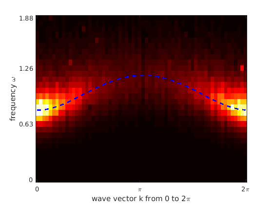
Figure 1: $S(\omega,k)$ of transverse field Ising chain $\Delta=1.0,J=0.2$ with no dissipation, $\alpha=0$. The recovered spectrum is compared with the exact result (the dashed blue curve).

The broadening is due to two reasons (1) finite size (classical $N_{0}=128$) or the finite temperature effects (quantum $T=1/\beta=1/N_{0}$) ; (2) our current Monte Carlo imaginary time correlation function has 5 significant digits (relative error $10^{-5}$), which is still a large error.

IV.2 Spectrum with dissipation

We turn on the dissipative strengths to be $\alpha=0.05,0.1,0.2,0.3,0.5$. Fig. (3 4 5 6 7 ) are the spectral plots for individual $k$. Fig. ( 8 9 10 11 12) are the corresponding density plots of $S(\omega,k)$. From these results, we can see that as the dissipation strength is increased, the energy peak is shifted down. The energy distributions also get broadened, implying shorter life time of the quasi-particle excitation.

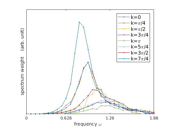
Figure 2: Transverse field Ising chain $\Delta=1.0,J=0.2$ with no dissipation $\alpha=0$. Each curve is $S(\omega,k)$ with fixed $k$ value.

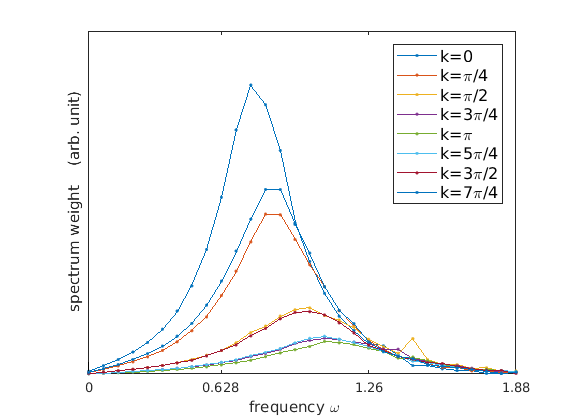
Figure 3: Transverse field Ising chain $\Delta=1.0,J=0.2$ with dissipation $\alpha=0.05$. Each curve is $S(\omega,k)$ with fixed $k$ value.

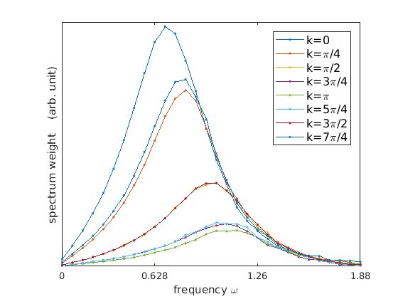
Figure 4: Transverse field Ising chain $\Delta=1.0,J=0.2$ with dissipation $\alpha=0.1$. Each curve is $S(\omega,k)$ with fixed $k$ value.

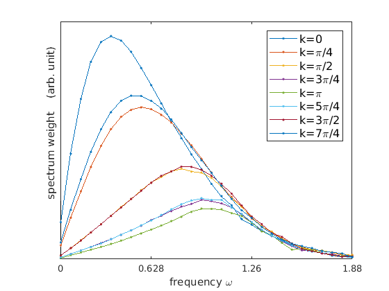
Figure 5: Transverse field Ising chain $\Delta=1.0,J=0.2$ with dissipation $\alpha=0.2$. Each curve is $S(\omega,k)$ with fixed $k$ value.

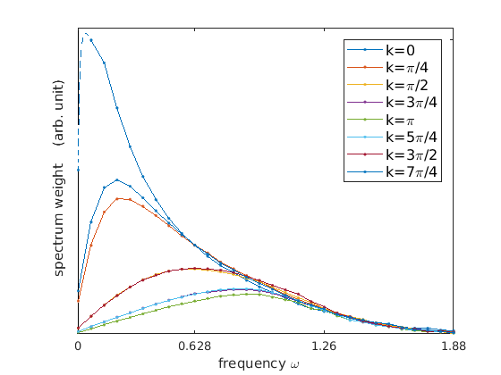
Figure 6: Transverse field Ising chain $\Delta=1.0,J=0.2$ with dissipation $\alpha=0.3$. Each curve is $S(\omega,k)$ with fixed $k$ value. The $k=0$ curve changes violently near zero frequency, we use dashed line to interpolate.

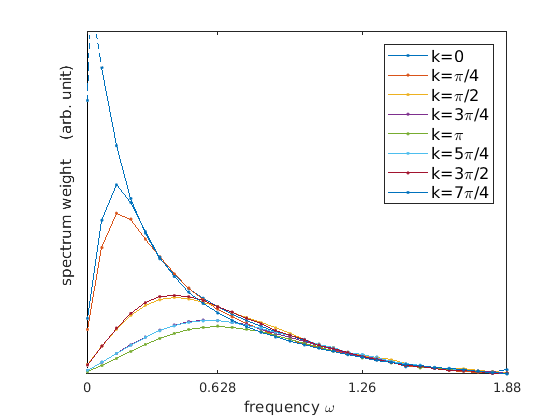
Figure 7: Transverse field Ising chain $\Delta=1.0,J=0.2$ with dissipation $\alpha=0.5$. Each curve is $S(\omega,k)$ with fixed $k$ value. The $k=0$ curve changes violently near zero frequency, the peak will be out of the graph. We use dashed line to interpolate.

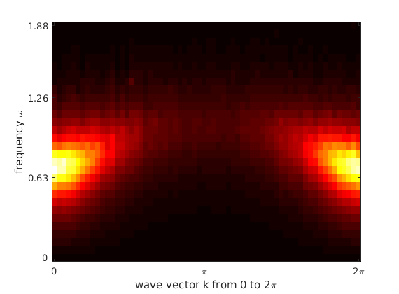
Figure 8: $S(\omega,k)$ of transverse field Ising chain $\Delta=1.0,J=0.2$ with dissipation $\alpha=0.05$.

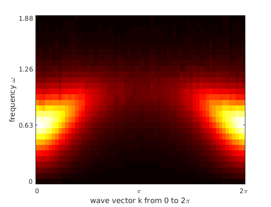
Figure 9: $S(\omega,k)$ of transverse field Ising chain $\Delta=1.0,J=0.2$ with dissipation $\alpha=0.1$.

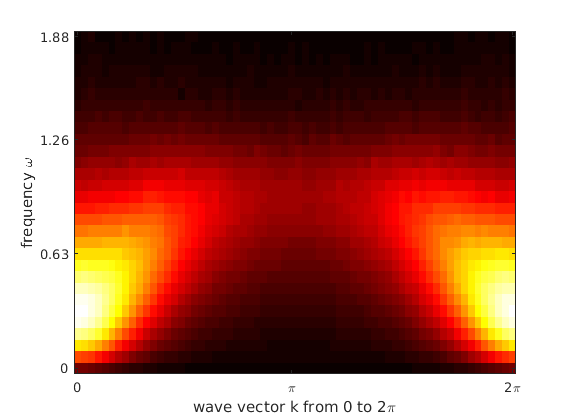
Figure 10: $S(\omega,k)$ of transverse field Ising chain $\Delta=1.0,J=0.2$ with dissipation $\alpha=0.2$.

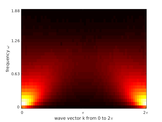
Figure 11: $S(\omega,k)$ of transverse field Ising chain $\Delta=1.0,J=0.2$ with dissipation $\alpha=0.3$.

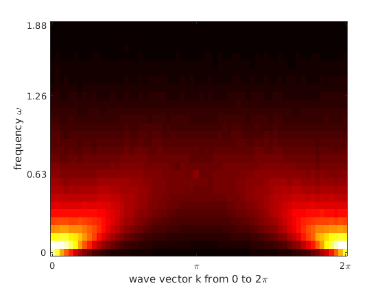
Figure 12: $S(\omega,k)$ of transverse field Ising chain $\Delta=1.0,J=0.2$ with dissipation $\alpha=0.5$.

The energy gap is more subtle. Only in the non-dissipative system, can we observe a clean energy gap. As the dissipation is turned on a little bit, it forms a pseudo-gap, and closes softly. At low energies $S(\omega)\propto\omega^{\delta}$, we can classify the gap closing into three cases: $\delta>1$ soft closing, $\delta=1$ linear closing, $\delta<1$ hard closing. The low energy exponent $\delta=\delta(\alpha,k)$ is a function of dissipation strength $\alpha$, and momentum $k$.

For $\alpha=0.1$, see Fig 4. The spectral curve is convex at low energy for all momentum. $\delta(0.1,k)<1$ For $\alpha=0.2$, see Fig 5. It’s very interesting. At low momentum, the spectrum is convex $\delta>1$, while at high momentum, the spectrum is concave $\delta<1$. And there exist a special momentum $k_{c}$ such that the dispersion is linear $\delta(\alpha,k_{c})=1$, which divides the convex and concave regions. (in the $\alpha=0.2$ case, it is $k_{c}\approx\frac{\pi}{2},\pi$) For $\alpha=0.3$, see Fig 6. The spectrum shifts to low frequency and the gap is closing. The low energy shape is concave ($\delta<1$) for all momenta.

IV.3 Three dynamical phases

As dissipation is turned on, the low momentum spectrum gets damped faster than the high momentum, in terms of the $\delta$ value. Therefore we can classify the system into three different regions:

1. Weakly damped region

2. Linear $k$-edge region

3. Strongly damped region

In Fig 13, the schematics of these three regions are plotted. Fig 14 is the phase diagram. The light yellow and grey region correspond to the magnetically disordered and ordered phases in the imaginary time simulation. Green, red, blue dots correspond to the three dynamical phases of the real time spectra.

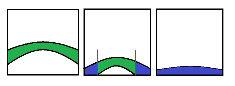
Figure 13: A schematic showing three dynamical phases (from left to right: weak damped $\alpha=0.1$, linear k-edge $\alpha=0.2$, strong damped $\alpha=0.3$ ). The horizontal axis is $k$, the vertical axis is $\omega$, same as Fig. (9,10,11). The band is colored green if $\delta(k)>1$ , blue if $\delta(k)<1$ and red if $\delta(k)=1$.

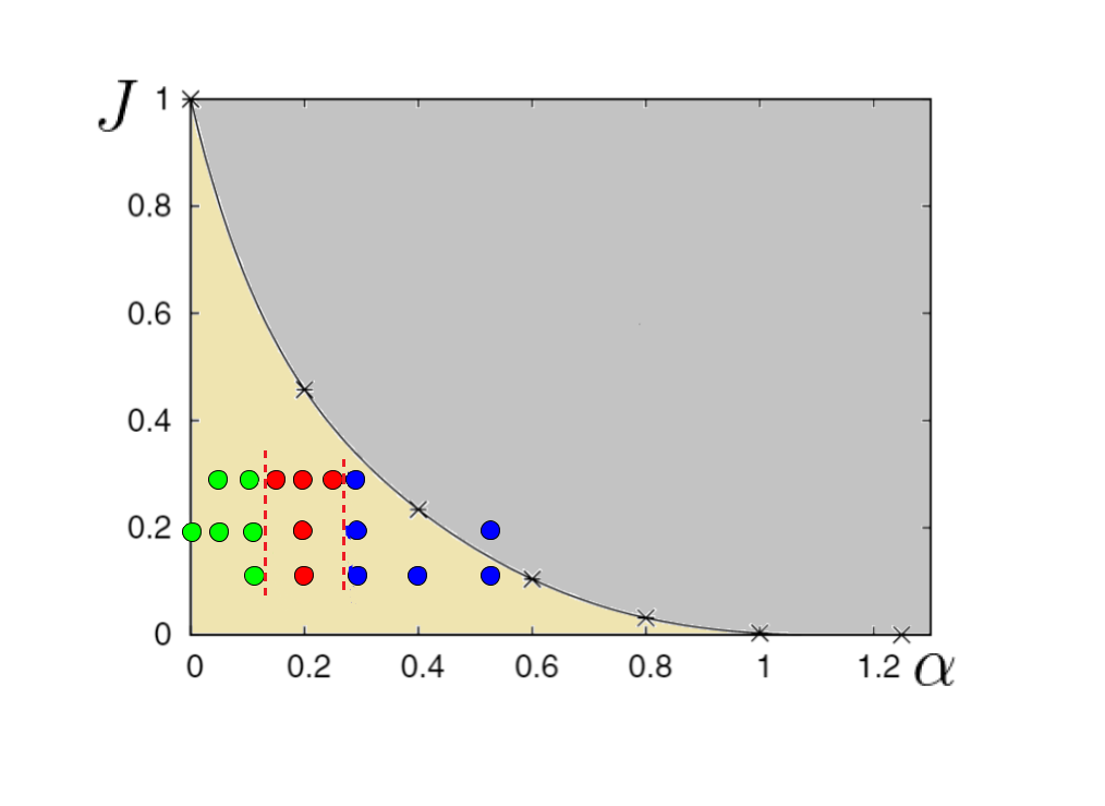
Figure 14: Phase diagram of dissipative Ising chain. Vertical axis $J$ is the nearest neighbour $\sigma^{z}_{i}\sigma^{z}_{i+1}$coupling, horizontal axis $\alpha$ is the dissipation strength, transverse field is set to $\Delta=1$ or $K_{0}=0.136$. The yellow and grey regions are the disordered and ordered magnetic phases from the imaginary time simulation Werner et al. (2005a). Green, red, and blue dots represent weakly damped, linear $k$-edge, and strongly damped regions respectively.

In the limit of zero dissipation, it is the transverse field Ising model, which is an integrable system. For each $k$ the excitation has infinite life time. In the limit of large dissipation, the Hamiltonian is dominated by the environmental noise term. The quasi-particles will decay faster than its energy time scale. In the intermediate dissipation range, low momentum will not have quasi-particle excitation, while high momentum will. The critical damping edge momentum $k_{c}$, is given by $S(\alpha,\omega,k_{c})\propto\omega$.

V Conclusion

To summarize, we have used extensive quantum Monte Carlo simulation, plus the rational function (Padé) regression method to recover the spectra of the dissipative Ising chain. As the dissipation strength is increased, the spectral speak is broadened and lowered in energy. Quasi-particle picture $S(\omega,k)=\delta(\omega-\omega(k))$ does not hold; $\frac{1}{\omega-\omega^{\prime}(k)-i\omega^{\prime\prime}(k)}$ is generalized to an arbitrary rational function. According to lower energy exponent of $S(\omega,k)\sim\omega^{\delta(k)}$ three dynamical regions are introduced to understand the role of dissipation.