Attacking Graph-based Classification via Manipulating the Graph Structure

Abstract.

Graph-based classification methods are widely used for security analytics. Roughly speaking, graph-based classification methods include collective classification and graph neural network. Attacking a graph-based classification method enables an attacker to evade detection in security analytics. However, existing adversarial machine learning studies mainly focused on machine learning for non-graph data. Only a few recent studies touched adversarial graph-based classification methods. However, they focused on graph neural network, leaving collective classification largely unexplored.

We aim to bridge this gap in this work. We consider an attacker’s goal is to evade detection via manipulating the graph structure. We formulate our attack as a graph-based optimization problem, solving which produces the edges that an attacker needs to manipulate to achieve its attack goal. However, it is computationally challenging to solve the optimization problem exactly. To address the challenge, we propose several approximation techniques to solve the optimization problem. We evaluate our attacks and compare them with a recent attack designed for graph neural networks using four graph datasets. Our results show that our attacks can effectively evade graph-based classification methods. Moreover, our attacks outperform the existing attack for evading collective classification methods and some graph neural network methods.

1. Introduction

Graph-based classification methods have been widely applied to various security problems such as malware detection (Chau et al., 2011; Tamersoy et al., 2014), fraudulent user detection in social networks (Yu et al., 2008; Yang et al., 2012; Cao et al., 2012; Jia et al., 2017a; Gong et al., 2014a; Wang et al., 2017b, 2018b), fake review detection (Akoglu et al., 2013; Wang et al., 2019), auction fraud detection (Pandit et al., 2007), APT infection detection (Oprea et al., 2015), and attribute inference (Gong et al., 2014b; Gong and Liu, 2016; Jia et al., 2017b). Specifically, given 1) a graph (undirected or directed) and 2) a training dataset (some labeled positive nodes and labeled negative nodes), a graph-based classification method predicts the unlabeled nodes in the graph to be either positive or negative. The semantics of the graph, positive, and negative are different in different security problems. For instance, in fraudulent user detection, the graph could be a friendship graph where nodes are users and edges represent friendship between users, while positive means fraudulent user and negative means normal user.

Roughly speaking, there are two types of graph-based classification methods, i.e., collective classification (Yu et al., 2008; Cao et al., 2012; Yang et al., 2012; Li et al., 2013; Boshmaf et al., 2015; Jia et al., 2017a; Pandit et al., 2007; Chau et al., 2011; Gong et al., 2014a; Tamersoy et al., 2014; Akoglu et al., 2013; Gao et al., 2018; Wang et al., 2017b, a, 2018a, 2019) and graph neural network (Scarselli et al., 2009; Weston et al., 2012; Kipf and Welling, 2017; Battaglia et al., 2018). Collective classification defines a prior reputation score to each node based on the training dataset, assigns certain weights to edges, and propagates the prior reputation scores among the weighted graph to obtain a posterior reputation score for each node. The posterior reputation scores are used to classify nodes. For instance, certain state-of-the-art collective classification methods assign the same weight to all edges and use Linearized Loopy Belief Propagation (LinLBP) to propagate the reputation scores (Jia et al., 2017b; Wang et al., 2017a). Graph neural network generalizes neural networks to graph data. These methods learn feature vectors for nodes based on the graph structure and use them to classify nodes. For certain security problems, collective classification outperforms graph neural network (Wang et al., 2019). Moreover, collective classification methods were deployed in industry for malware detection (Chau et al., 2011; Tamersoy et al., 2014) and fraudulent user detection in social networks (Cao et al., 2012; Boshmaf et al., 2015).

As graph-based classification methods are adopted to enhance security, an attacker is motivated to evade them. However, existing studies (Nelson et al., 2010; Huang et al., 2011; Biggio et al., 2013; Srndic and Laskov, 2014; Szegedy et al., 2013; Goodfellow et al., 2014; Papernot et al., 2016a; Xu et al., 2016; Carlini et al., 2016; Sharif et al., 2016; Liu et al., 2017; Biggio et al., 2012; Xiao et al., 2015; Li et al., 2016; Yang et al., 2017; Jagielski et al., 2018a; Fang et al., 2018; Fredrikson et al., 2015; Shokri et al., 2017; Pyrgelis et al., 2018; Ganju et al., 2018; Tramèr et al., 2016; Ji et al., 2018; Wang and Gong, 2018) on adversarial machine learning mainly focused on machine learning for non-graph data, with only a few studies (Torkamani and Lowd, 2013; Liu et al., 2015; Chen et al., 2017; Dai et al., 2018b; Sun et al., 2018; Dai et al., 2018a; Zügner et al., 2018; Bojchevski and Günnemann, 2019; Zügner and Günnemann, 2019a, b) as exceptions. In particular, Chen et al. (Chen et al., 2017) proposed an attack against graph-based clustering, e.g., spectral clustering. Several recent work (Dai et al., 2018b; Zügner et al., 2018; Sun et al., 2018; Dai et al., 2018a; Bojchevski and Günnemann, 2019; Zügner and Günnemann, 2019a) proposed attacks to graph neural network methods via manipulating the graph structure, i.e., inserting fake edges to the graph or deleting existing edges. However, collective classification under adversarial setting is largely unexplored.

Our work: In this work, we study attacks to collective classification via manipulating the graph structure. We generate the fake edges and the deleted edges based on the collective classification method LinLBP, because 1) LinLBP achieves state-of-the-art performance, and 2) LinLBP uses the same weight for all edges, making our formulated optimization problem easier to solve. However, we will empirically show that our attacks based on LinLBP can also transfer to other collective classification methods and graph neural network methods, as they all leverage the graph structure.

We consider an attacker has some positive nodes (e.g., malware, fraudulent users, fake reviews) and aims to spoof LinLBP to misclassify them as negative via manipulating the graph structure. In other words, the attacker aims to increase the False Negative Rate (FNR) of its positive nodes. We propose to characterize the attacker’s background knowledge along three dimensions: Parameter, Training dataset, and Graph, which characterize whether the attacker knows the parameters (i.e., prior reputation scores and edge weights) used by LinLBP, the training dataset, and the complete graph, respectively. Inserting/Deleting different edges may incur different costs to the attacker. For instance, inserting an edge between the attacker’s positive nodes is less expensive than inserting an edge between two negative nodes that are not under the attacker’s control. Therefore, we associate a (different) cost for inserting or deleting each edge. The attacker’s goal is to achieve a high FNR (e.g., FNR=1) for its positive nodes with a minimal total cost of inserting/deleting edges.

We formulate our attack as an optimization problem, where the objective function is the total cost of modifying the graph structure and the constraint is FNR=1 for the attacker’s selected positive nodes. However, it is computationally challenging to solve such an optimization problem because 1) the constraint is highly nonlinear and 2) the optimization problem is a binary optimization problem (inserting or deleting an edge is a binary decision). We propose several techniques to approximately solve the optimization problem. For instance, we relax the binary variables in the optimization problem to be continuous variables and convert them to binary values after solving the optimization problem; we use posterior reputation scores as an alternative to FNR and translate the constraint FNR=1 into the objective function via Lagrangian multipliers; and we propose to alternately solve the optimization problem and compute the posterior reputation scores.

We first extensively evaluate our attacks using three real-world graphs with synthesized positive nodes and a real-world large-scale Twitter graph with real positive nodes. Our attacks are effective, e.g., our attacks can increase the FNR from 0 to be above 0.90 in many cases. Our attack is still effective even if the attacker does not have access to the parameters of LinLBP (our attack can use substitute parameters), the training dataset (our attack can use a substitute training dataset), and the complete graph (a 20% partial graph is sufficient). Second, our attacks can also transfer to other collective classification methods including random walk based methods (Jia et al., 2017a), Loopy Belief Propagation based methods (Gong et al., 2014a), and recent Joint Weight Learning and Propagation method (Wang et al., 2019) that learns edge weights, as well as graph neural network methods including Graph Convolutional Network (GCN) (Kipf and Welling, 2017), LINE (Tang et al., 2015), DeepWalk (Perozzi et al., 2014), and node2vec (Grover and Leskovec, 2016). Third, we compare our attack with a recent attack called Nettack (Zügner et al., 2018) that generates fake edges and deleted edges based on GCN. We find that for GCN, Nettack outperforms our attack; for other graph neural network methods, our method outperforms Nettack; and for collective classification methods, our attack substantially outperforms Nettack.

Our contributions can be summarized as follows:

• We perform the first systematic study on attacks to collective classification via manipulating the graph structure.

• We propose a threat model of attacking collective classification, formulate our attack as an optimization problem, and propose techniques to approximately solve the problem.

• We extensively evaluate our attacks and compare them with a recent attack using multiple datasets.

2. Related Work

2.1. Graph-based Classification Methods

Roughly speaking, there are two types of graph-based classification methods, i.e., collective classification and graph neural network.

2.1.1. Collective Classification

Collective classification has been applied for graph-based security analytics for over a decade. Specifically, given a training dataset, collective classification first defines a prior reputation score for each node in the graph. Then, it assigns or learns weights for the edges in the graph and propagates the prior reputation scores among the graph to obtain a posterior reputation score for each node. The posterior reputation scores are used to classify unlabeled nodes. Different collective classification methods use different ways to define the prior reputation scores, assign/learn the edge weights, and propagate the prior reputation scores. In particular, state-of-the-art collective classification methods include Random Walk (RW) based methods (Zhu et al., 2003; Gyöngyi et al., 2004; Yu et al., 2008; Cao et al., 2012; Yang et al., 2012; Li et al., 2013; Boshmaf et al., 2015; Jia et al., 2017a), Loopy Belief Propagation (LBP) based methods (Pandit et al., 2007; Chau et al., 2011; Gong et al., 2014a; Tamersoy et al., 2014; Akoglu et al., 2013; Gao et al., 2018), Linearized Loopy Belief Propagation (LinLBP) based methods (Jia et al., 2017b; Wang et al., 2017a), and Joint Weight Learning and Propagation (JWP) method (Wang et al., 2019).

RW-based methods assign prior reputation scores 1, 0, and 0.5 to the labeled positive nodes, labeled negative nodes, and unlabeled nodes, respectively. Moreover, they assign the same weight (e.g., (Zhu et al., 2003)) or weights learnt using node attributes (e.g., (Boshmaf et al., 2015)) to edges. Finally, they leverage random walk to propagate the reputation scores in the weighted graph. In particular, they iteratively distribute a node’s current reputation score to its neighbors in proportion to the edge weights, and a node sums the reputation scores from its neighbors as the new reputation score. LBP-based methods often assign the same weight for all edges. Moreover, they model the graph as a pairwise Markov Random Fields and leverage the standard LBP to perform inference, which obtains the posterior reputation scores. However, LBP has two well-known limitations: not guaranteed to converge for loopy graphs and not scalable (because it maintains messages on each edge). LinLBP linearizes LBP to address the two limitations. We will discuss details of LinLBP in Section 3.1. LinLBP and LBP based methods were shown to outperform RW-based methods (Jia et al., 2017b; Wang et al., 2018a).

JWP (Wang et al., 2019) jointly learns edge weights and propagates reputation scores. Given the current posterior reputation scores, JWP learns edge weights such that 1) the labeled positive nodes and labeled negative nodes have large and small posterior reputation scores in the next iteration, respectively, and 2) an edge has a large weight if the two corresponding nodes are predicted to have the same label using its current posterior reputation scores, otherwise the edge has a small weight. Given the learnt edge weights, JWP computes the posterior reputation scores in the next iteration, e.g., using LinLBP-based propagation. JWP outperforms LinLBP (Wang et al., 2019). However, attacking JWP directly is challenging because JWP learns edge weights. Specifically, when we insert fake edges to the graph or delete existing edges, the impact of these inserted/deleted edges on the classification of the attacker’s positive nodes relies on the edge weights that need to be re-learnt by JWP. Therefore, we will focus on attacking LinLBP and empirically show that our attacks also transfer to RW-based methods, LBP-based methods, and JWP.

2.1.2. Graph Neural Network

These methods generalize neural networks to graph data. In particular, they learn feature vectors for nodes using neural networks and use them to classify nodes.

Some graph neural network methods (Scarselli et al., 2009; Weston et al., 2012; Kipf and Welling, 2017; Battaglia et al., 2018) learn the node feature vectors and classify nodes simultaneously. Roughly speaking, in these methods, neurons in the hidden layers of a neural network represent feature vectors of nodes, which are used to classify nodes in the last layer of the neural network. The architecture of the neural network is determined by the graph structure, e.g., a neuron in a layer that models a certain node is connected with the neurons in the previous layer that model the node’s neighbors. In other words, the neural network iteratively computes a feature vector of a node via aggregating the feature vectors of the node’s neighbors. The neural network parameters are learnt via minimizing a graph-based loss function on both labeled nodes in the training dataset and the remaining unlabeled nodes. In particular, the graph-based loss function is small if nodes sharing the same label have similar feature vectors and nodes having different labels have distinct feature vectors. For instance, Graph Convolutional Network (GCN) (Kipf and Welling, 2017) leverages spectral graph convolutions (Defferrard et al., 2016) in a neural network to learn feature vectors, and adopts a logistic regression classifier in the last layer.

Some graph neural network methods (Perozzi et al., 2014; Tang et al., 2015; Cao et al., 2015; Grover and Leskovec, 2016) first learn feature vectors for nodes in an unsupervised learning fashion (also known as graph embedding); then they use the feature vectors and the training dataset to learn a standard binary classifier (e.g., logistic regression); and finally they use the classifier to predict labels for the unlabeled nodes. Different methods learn the feature vectors using different techniques. For instance, DeepWalk (Perozzi et al., 2014) learns feature vectors via generalizing the word to vector technique developed for natural language processing to graph data. In particular, DeepWalk treats a node as a word in natural language, generates node sequences (like sentences in natural language) using truncated random walks, and leverages the skip-gram model (Mikolov et al., 2013) to learn a feature vector for each node. LINE (Tang et al., 2015) learns nodes’ feature vectors by preserving both first-order and second-order proximity, where the first-order proximity captures the links in the graph (e.g., the first-order proximity between two nodes is 0 if they are not connected) and the second-order proximity between two nodes captures the similarity between their neighborhoods.

2.2. Adversarial Graph-based Machine Learning

Existing studies on adversarial machine learning mainly focused on machine learning for non-graph data. In particular, studies have demonstrated that machine learning is vulnerable to adversarial examples (Nelson et al., 2010; Huang et al., 2011; Biggio et al., 2013; Srndic and Laskov, 2014; Szegedy et al., 2013; Goodfellow et al., 2014; Papernot et al., 2016a; Xu et al., 2016; Carlini et al., 2016; Sharif et al., 2016; Liu et al., 2017; Jia and Gong, 2018), poisoning attacks (Biggio et al., 2012; Xiao et al., 2015; Li et al., 2016; Yang et al., 2017; Jagielski et al., 2018a; Fang et al., 2018), privacy attacks for users (e.g., model inversion attacks (Fredrikson et al., 2014; Fredrikson et al., 2015), membership inference attacks (Shokri et al., 2017; Pyrgelis et al., 2018), property inference attacks (Ateniese et al., 2015; Ganju et al., 2018)), as well as model parameter and hyperparameter stealing attacks (Tramèr et al., 2016; Wang and Gong, 2018).

Graph-based machine learning under adversarial setting is much less explored. In particular, only a few studies  (Torkamani and Lowd, 2013; Chen et al., 2017; Dai et al., 2018b; Sun et al., 2018; Dai et al., 2018a; Zügner et al., 2018; Bojchevski and Günnemann, 2019; Zügner and Günnemann, 2019a; Liu et al., 2015) focused on adversarial graph-based machine learning. For instance, Chen et al. (Chen et al., 2017) proposed a practical attack against graph-based clustering, e.g., spectral clustering. Torkamani and Lowd (Torkamani and Lowd, 2013) proposed an attack to associative Markov network-based classification methods. However, they considered that an attacker manipulates up to a fixed number of binary-valued node attributes instead of manipulating the graph structure. Several work (Dai et al., 2018b; Zügner et al., 2018; Sun et al., 2018; Bojchevski and Günnemann, 2019; Zügner and Günnemann, 2019a) proposed attacks to graph neural network methods via inserting fake edges to the graph or deleting existing edges. For instance, Zügner et al. (Zügner et al., 2018) proposed an attack called Nettack against GCN (Kipf and Welling, 2017). First, Nettack defines a graph structure preserving perturbation, which constrains that the node degree distributions of the graph before and after attack should be similar. Then, Nettack learns a surrogate linear model of GCN. Finally, Nettack generates fake/deleted edges via maximizing a surrogate loss function with respect to the graph structure, where the optimization problem is subject to the node degree distribution constraint. Several recent works (Zügner and Günnemann, 2019b; Bojchevski and Günnemann, 2019; Zügner and Günnemann, 2019a) further studied attacks and defenses for graph neural networks, which are concurrent to our work.

Our attack is designed for collective classification and is complementary to existing attacks that target graph neural networks.

3. Background and Problem Setup

3.1. Linearized Loopy Belief Propagation

Suppose we are given an undirected graph $G=(V,E)$, where $u\in V$ is a node and $(u,v)\in E$ is an edge. $|V|$ and $|E|$ are the number of nodes and edges, respectively. Moreover, we have a training dataset $L$, which consists of a set of labeled positive nodes $L_{P}$ and a set of labeled negative nodes $L_{N}$. LinLBP (Jia et al., 2017b) assigns the prior reputation score $q_{u}$ for a node $u$ as follows:

(1) $$q_{u}=\begin{cases}\theta&\text{ if }u\in L_{P}\\ -\theta&\text{ if }u\in L_{N}\\ 0&\text{ otherwise, }\end{cases}$$

where $0<\theta\leq 1$ is a parameter of LinLBP. LinLBP assigns the same weight $w$ in the interval (0, 0.5] for all edges. A larger weight means that two linked nodes are more likely to have the same label. We denote by $\mathbf{A}$ the adjacency matrix of the graph, and by $\mathbf{W}$ a $|V|\times|V|$ matrix, every entry of which is the weight $w$. Then, the posterior reputation scores in LinLBP are a solution of the following system:

(2) $$\mathbf{p}={\mathbf{q}}+{\mathbf{A}\odot\mathbf{W}}{\mathbf{p}},$$

where $\mathbf{q}$ and $\mathbf{p}$ are the column vector of prior reputation scores and posterior reputation scores of all nodes, respectively. $\odot$ means element-wise product of two matrices. We note that $\mathbf{A}\odot\mathbf{W}$ essentially is the weight matrix of the graph. However, as we will see in the next section, splitting the weight matrix into the element-wise produce of $\mathbf{A}$ and $\mathbf{W}$ makes it easier to present our techniques to solve the optimization problem that models our attack. The posterior reputation scores are iteratively computed as follows:

(3) $$\mathbf{p}^{(t)}={\mathbf{q}}+{\mathbf{A}\odot\mathbf{W}}{\mathbf{p}^{(t-1)}},$$

where $\mathbf{p}^{(t)}$ is the column vector of posterior reputation scores in the $t$th iteration. When the posterior reputation scores converge, a node $u$ is predicted to be negative if its posterior reputation score is negative, i.e., $p_{u}<0$. We note that LinLBP has two parameters, i.e., the prior reputation score parameter $\theta$ and the edge weight $w$.

3.2. Threat Model

Attacker’s background knowledge:  A LinLBP system is characterized by three major components: parameters of LinLBP, a training dataset $L$, and a graph $G=(V,E)$. Therefore, we characterize an attacker’s background knowledge along three dimensions:

• Parameter. This dimension characterizes whether the attacker knows the parameters (i.e., $\theta$ and $w$) of LinLBP.

• Training. This dimension characterizes whether the attacker knows the training dataset.

• Graph. This dimension characterizes whether the attacker knows the complete graph.

For convenience, we denote an attacker’s background knowledge as a triple (Parameter, Training, Graph), where Parameter can be Yes or No, Training can be Yes or No, and Graph can be Complete or Partial. For instance, a triple (Yes, Yes, Complete) means that the attacker (e.g., an insider) knows the parameters, the training dataset, and the complete graph. An attacker knows its positive nodes and edges between them. An attacker could also know a subgraph of the negative nodes. For instance, in social networks, an attacker can develop a web crawler to collect a partial social graph of the negative nodes (i.e., normal users). We will empirically show that our attack is still effective even if the attacker uses substitute parameters, a substitute training dataset, and a partial graph.

Attacker’s capability:  We consider an attacker can change the graph structure, i.e., the attacker can insert fake edges to the graph or delete existing edges. For instance, in social networks, an attacker can create new edges among its created fraudulent users (positive nodes) or remove existing edges between its created fraudulent users. In addition, an attacker may also compromise normal users (negative nodes) and create edges between the compromised users and its fraudulent users. However, adding or removing different edges may incur different costs for the attacker. For instance, in the fraudulent user detection problem, adding an edge between two fraudulent users requires a smaller cost than adding an edge between a fraudulent user and a compromised normal user, as an attacker usually needs an extra effort to compromise a normal user. Thus, we associate a cost with inserting/deleting each edge, where the costs may depend on different security applications. Moreover, in certain applications, the maximum number of edges that can be inserted/deleted for a node is bounded. For instance, in online social networks, the number of friends (i.e., edges) a user can have is often bounded. Thus, we introduce a parameter $K$, which is the maximum number of edges that can be inserted/deleted for a node.

Attacker’s goal:  Suppose an attacker has some selected positive nodes (e.g., malware, fraudulent user, fake review), which we call target nodes. We consider the attacker’s goal is to make the target nodes evade the detection of LinLBP. Specifically, the attacker aims to manipulate the graph structure with a minimal total cost such that LinLBP misclassifies the target nodes to be negative. In other words, the attacker’s goal is to achieve a high False Negative Rate (FNR) for its target nodes via manipulating the graph structure with a minimal total cost. We note that the target nodes may be a subset of the positive nodes under the attacker’s control.

3.3. Problem Definition

Given our threat model, we formally define our problem as follows:

Definition 3.1 (Attack to LinLBP).

Given some target nodes, attacker’s background knowledge, cost of inserting/deleting each edge, and the maximum number of inserted/deleted edges for each node, an attack to LinLBP is to manipulate the graph structure with a minimal total cost such that LinLBP achieves a as high FNR for the target nodes as possible.

4. Our Attacks

We first discuss our attacks under the threat model where the attacker has full knowledge, i.e., the attacker knows the parameters of LinLBP, the training dataset, and the complete graph. Then, we adjust our attacks to the scenarios where the attacker only has partial knowledge about the parameters, the training dataset, and/or the graph.

4.1. Adversary with Full Knowledge

Overview:  We first formulate our attack as an optimization problem. Specifically, we associate a binary variable with each pair of nodes, where a binary variable has a value of 1 if and only if our attack changes the connection state between the corresponding two nodes. The objective function of the optimization problem is the total cost of manipulating the graph structure and the constraints are 1) FNR=1 for the attacker’s target nodes and 2) the maximum number of inserted/deleted edges per node is bounded by $K$. However, it is computationally challenging to solve the optimization problem because it is a binary optimization problem that has $O(|V|^{2})$ binary variables and the constraint FNR=1 is highly nonlinear.

To address the challenges, we propose techniques to approximately solve the optimization problem. Specifically, we relax the binary variables to continuous variables whose values are in the interval [0, 1] and convert them to binary values after solving the optimization problem; and we reduce the optimiztion to the binary variables that are related to the attacker’s target nodes. Moreover, we translate the constraint FNR=1 to be a constraint on the posterior reputation scores of the attacker’s target nodes and add the constraint to the objective function using Lagrangian multipliers. However, the converted optimization problem still faces a computational challenge because the posterior reputation scores depend on the graph structure (i.e., the continuous variables in the optimization problem) in a complex way, i.e., each variable could influence the posterior reputation score of each node. To address the challenge, we propose to alternately optimize the continuous variables in the optimization problem and compute the posterior reputation scores. Our key idea is that posterior reputation scores are computed iteratively. Instead of using the final posterior reputation scores, we use the intermediate posterior reputation scores to optimize the continuous variables in the optimization problem.

Formulating our attack as an optimization problem: We associate a binary variable $B_{uv}$ with each pair of nodes $u$ and $v$. $B_{uv}=1$ if our attack changes the connection state between $u$ and $v$, otherwise $B_{uv}=0$. Specifically, if $u$ and $v$ are already connected in the original graph, then $B_{uv}=1$ if our attack deletes the edge between $u$ and $v$; if $u$ and $v$ are not connected in the original graph, then $B_{uv}=1$ if our attack inserts an edge between $u$ and $v$. As we discussed in our threat model in Section 3.2, inserting/deleting different edges may incur different costs for the attacker. Therefore, we associate a variable $C_{uv}$ with each pair of nodes $u$ and $v$ to represent the cost of modifying the connection state between $u$ and $v$. In particular, $B_{uv}=1$ incurs a cost $C_{uv}$ for the attacker. Therefore, the total cost of an attack is $\sum_{u,v\in V,u<v}B_{uv}C_{uv}$, where $V$ is the set of nodes in the graph and the constraint $u<v$ essentially means that we count once for each pair of nodes. We note that, for the same node pair, we could also associate different costs for inserting an edge and deleting the existing edge between them. Our method is also applicable for such fine-grained cost. However, for simplicity, we use the same cost for inserting/deleting an edge.

The attacker has a set of selected target nodes $\mathcal{T}$ and aims to achieve a high FNR (i.e., FNR=1 in our formulation) for the target nodes with a minimal total cost. Formally, our attack aims to find the variables $B_{uv}$ via solving the following optimization problem:

(4) $$\min_{\mathbf{B}}\sum_{u,v\in V,u<v}B_{uv}C_{uv},$$

(5) $$\textrm{s.t.}\quad FNR=1,$$

(6) $$\quad\quad B_{uv}\in\{0,1\},\text{ for }u,v\in V,$$

(7) $$\quad\quad\sum_{v}B_{uv}\leq K,\text{ for }u\in V,$$

where the symmetric matrix $\mathbf{B}$ includes all the binary variables for each pair of nodes, the objective function is the total cost, the first constraint means all target nodes are misclassified as negative, the second constraint means the variables in the optimization problem are binary, and the third constraint means the maximum number of inserted/deleted edges for each node is bounded by $K$. For convenience, we call the matrix $\mathbf{B}$ adversarial matrix.

Challenges for solving the optimization problem:  Solving the optimization problem in Equation 4 exactly faces several challenges. First, the variables $B_{uv}$ are binary. Second, the optimization problem has $|V|(|V|-1)/2$ binary variables. Third, the constraint FNR=1 is highly nonlinear.

Our techniques for approximately solving the optimization problem:  We propose several approximation techniques to address the challenges. To address the first challenge, we relax $B_{uv}$ to a continuous variable whose value is in the interval [0, 1] and convert it to a binary value after solving the optimization problem.

In practice, it is often expensive to modify the connection states between negative nodes not under the attacker’s control. Thus, to address the second challenge, we reduce the optimization space to the edges between the attacker’s target nodes and the remaining nodes and the edges between the target nodes. Specifically, we solve the optimization problem over the variables related to the attacker’s target nodes, i.e., the variables $B_{uv}$ where ${\small u\in\mathcal{T},v\in V-\mathcal{T}}$ and $B_{uv}$ where ${\small u,v\in\mathcal{T},u<v}$, where the first set of variables characterize the connection states between the target nodes and the remaining nodes while the second set of variables characterize the connection states between the target nodes.

Recall that a node is predicted to be negative if its posterior reputation score is negative. Therefore, to address the third challenge, we replace the constraint FNR=1 as the constraint $p_{u}<0$ for each $u\in\mathcal{T}$. Moreover, we convert the constraint on posterior reputation scores to the objective function via Lagrangian multipliers. Summarizing our approximation techniques, we aim to solve the following optimization problem:

(8) $$\min_{\mathbf{B}}\mathcal{F}(\mathbf{B})=\sum_{u\in\mathcal{T},v\in V-\mathcal{T}}B_{uv}C_{uv}+\sum_{u,v\in\mathcal{T},u<v}B_{uv}C_{uv}+\lambda\sum_{u\in\mathcal{T}}p_{u}$$

(9) $$\textrm{s.t.}\quad B_{uv}\in[0,1],\text{ for }u\in\mathcal{T},v\in V$$

(10) $$\quad\quad\sum_{v}\bar{B}_{uv}\leq K,\text{ for }u\in V$$

where $\lambda>0$ is a Lagrangian multiplier, $\bar{B}_{uv}$ is the binarized value of the continuous variable $B_{uv}$, and the posterior reputation scores are a solution of the following system:

(11) $$\mathbf{p}={\mathbf{q}}+{|\mathbf{A}-\bar{\mathbf{B}}|\odot\mathbf{W}}{\mathbf{p}},$$

where $\mathbf{A}$ is the adjacency matrix of the original graph, $\bar{\mathbf{B}}$ is the binarized adversarial matrix, and $\mathbf{W}$ is a matrix with every entry as the edge weight $w$. ${\scriptsize|\mathbf{A}-\bar{\mathbf{B}}|}$ essentially is the adjacency matrix of the graph after our attack.

A popular method to solve the above optimization problem is to use gradient descent. However, it is still computationally challenging because the posterior reputation scores depend on the variables $\bar{\mathbf{B}}$ in a complex way, i.e., every variable $B_{uv}$ influences each posterior reputation score according to the system in Equation 11. To address the challenge, we propose to alternately optimize the variables in the optimization problem and compute the posterior reputation scores. Our key insight is that posterior reputation scores are iteratively computed. Instead of using the final posterior reputation scores, we use the intermediate posterior reputation scores to solve the optimization problem. Then, given the intermediate variables $B_{uv}$, we update the posterior reputation scores. Specifically, we repeat the following two steps.

Step I: updating posterior reputation scores. We update the posterior reputation scores in the $t$th iteration using the adversarial matrix ${\scriptsize\bar{\mathbf{B}}^{(t-1)}}$ in the $(t-1)$th iteration as follows:

(12) $$\mathbf{p}^{(t)}={\mathbf{q}}+{|\mathbf{A}-\bar{\mathbf{B}}^{(t-1)}|\odot\mathbf{W}}{\mathbf{p}^{(t-1)}}.$$

Step II: updating adversarial matrix. In this step, we update the adversarial matrix in the $t$th iteration while fixing the posterior reputation scores in the $t$th iteration. For convenience, we transform the optimization problem in Equation 8 to the following optimization problem:

(13) $$\min_{\mathbf{B}^{(t)}}\mathcal{F}(\mathbf{B}^{(t)})=\sum_{u\in\mathcal{T}}\mathbf{b}_{u}^{(t)}\mathbf{c}_{u}^{T}+\lambda\sum_{u\in\mathcal{T}}p_{u}^{(t+1)}$$

(14) $$\textrm{s.t.}\quad\mathbf{b}_{u}^{(t)}\in[0,1],\text{ for }u\in\mathcal{T}$$

(15) $$\quad\quad\sum_{v}\bar{B}_{uv}^{(t)}\leq K,\text{ for }u\in V$$

where ${\scriptsize\mathbf{b}_{u}^{(t)}}$ is the $u$th row of the matrix ${\small\mathbf{B}^{(t)}}$ (i.e., the modified connection states between a node $u$ and the remaining nodes), $\mathbf{c}_{u}$ is the adjusted $u$th row of the cost matrix $\mathbf{C}$, $T$ is transpose of a vector, and ${\scriptsize\mathbf{p}^{(t+1)}={\mathbf{q}}+{|\mathbf{A}-\bar{\mathbf{B}}^{(t)}|\odot\mathbf{W}}{\mathbf{p}^{(t)}}}$. Specifically, ${c}_{uv}=C_{uv}$ if $u\in\mathcal{T}$ and $v\notin\mathcal{T}$, while ${\small{c}_{uv}=C_{uv}/2}$ if $u,v\in\mathcal{T}$ (because each pair of nodes between the target nodes in $\mathcal{T}$ is counted twice in the objective function in Equation 13).

We use a projected gradient descent to solve the optimization problem in Equation 13. Specifically, we iteratively apply the following steps for each target node $u$:

(16) $${\mathbf{s}}_{u}^{(i+1)}=\tilde{\mathbf{b}}_{u}^{(i)}-\eta\frac{\partial\mathcal{F}(\tilde{\mathbf{B}}^{(i)})}{\partial\tilde{\mathbf{b}}_{u}^{(i)}},$$

(17) $$\tilde{\mathbf{b}}_{u}^{(i+1)}=\textrm{proj}\big{(}{\mathbf{s}}_{u}^{(i+1)}\big{)},$$

where the first equation means we update the variables $\tilde{\mathbf{b}}_{u}$ using gradient descent and the second equation means that we project the variables to satisfy the two constraints in Equation 14 and Equation 15. Note that the variables $\tilde{\mathbf{b}}_{u}$ are initialized using the adversarial matrix in the $(t-1)$th iteration, i.e., ${\scriptsize\tilde{\mathbf{b}}_{u}^{(0)}={\mathbf{\bar{b}}}_{u}^{(t-1)}}$. Specifically, the gradient can be computed as follows:

(18) $$\frac{\partial\mathcal{F}(\mathbf{\tilde{B}}^{(i)})}{\partial\mathbf{\tilde{b}}_{u}^{(i)}}=\mathbf{c}_{u}+\lambda\frac{\partial p_{u}^{(t+1)}}{\partial\mathbf{\tilde{b}}_{u}^{(i)}}=\mathbf{c}_{u}+\lambda\textrm{sign}(\mathbf{\tilde{b}}_{u}^{(i)}-\mathbf{a}_{u})\odot\mathbf{w}_{u}\mathbf{P}^{(t)},$$

where $\mathbf{a}_{u}$ is the $u$th row of the adjacency matrix, the sign operator applies to every entry of the vector ${\scriptsize\mathbf{\tilde{b}}_{u}^{(i)}-\mathbf{a}_{u}}$, and ${\scriptsize\mathbf{P}^{(t)}}$ is a diagonal matrix with the diagonal elements ${\scriptsize P_{u,u}^{(t)}=p_{u}^{(t)}}$. Note that when computing the gradient, we approximate ${\scriptsize\bar{\mathbf{B}}}$ as ${\scriptsize\tilde{\mathbf{B}}}$ in the computation of ${\scriptsize\mathbf{p}^{(t+1)}}$. Moreover, the operator proj is defined as follows:

(19) $$\textrm{proj}(\mathbf{s}_{u}^{(i+1)})=\operatornamewithlimits{argmin}_{0\leq\mathbf{\tilde{b}}_{u}^{(i+1)}\leq 1,\ \mathbf{\tilde{b}}_{u}^{(i+1)}\mathbf{1}^{T}\leq K}\|\mathbf{\tilde{b}}_{u}^{(i+1)}-\mathbf{s}_{u}^{(i+1)}\|_{2}^{2},$$

which means that the proj operator aims to find a vector ${\scriptsize\mathbf{\tilde{b}}_{u}^{(i+1)}}$ that is the closest to the vector ${\scriptsize\mathbf{s}_{u}^{(i+1)}}$ in terms of Euclidean distance and that satisfies the constraint ${\scriptsize 0\leq\mathbf{\tilde{b}}_{u}^{(i+1)}\leq 1}$ and a relaxed constraint ${\scriptsize\mathbf{\tilde{b}}_{u}^{(i+1)}\mathbf{1}^{T}\leq K}$ on the maximum number of inserted/deleted edges for node $u$. The optimization problem in Equation 19 can be solved exactly by the break point search method (Yuan and Ghanem, 2017). We repeat the Equation 16 and 17 multiple iterations to solve $\mathbf{\tilde{b}}_{u}$. However, more iterations make our method less efficient. In our experiments, we repeat 4 iterations to solve $\mathbf{\tilde{b}}_{u}$ as we find that 4 iterations achieve a good trade-off between accuracy and efficiency.

After solving $\mathbf{\tilde{b}}_{u}$ with 4 iterations, we convert them to be binary values. Specifically, we first convert each ${\tilde{b}}_{uv}$ to 1 if ${\tilde{b}}_{uv}>0.5$ and 0 otherwise. Then, we select the largest $K$ entries in $\mathbf{\tilde{b}}_{u}$ and convert them to be 1, while we convert the remaining entries in the vector to be 0. Finally, we assign the converted binary vector as the corresponding row $\mathbf{\bar{b}}_{u}^{(t)}$ in the adversarial matrix in the $t$th iteration. Note that such converted adversarial matrix may not be symmetric for the targeted nodes. Specifically, we may have $\bar{B}_{uv}\neq\bar{B}_{vu}$ for a pair of target nodes $u$ and $v$. Therefore, we perform another postprocessing for the edges between target nodes. Specifically, we set $\bar{B}_{uv}=\bar{B}_{vu}\leftarrow\bar{B}_{uv}\cdot\bar{B}_{vu}$, i.e., we modify the connection state between $u$ and $v$ only if both $\bar{B}_{uv}=1$ and $\bar{B}_{vu}=1$.

Computational complexity:  We first analyze the time complexity in one iteration. In Step I, updating posterior reputation scores traverses all edges in the graph and the time complexity is $O(|E|)$. In Step II, for each target node $u\in\mathcal{T}$, updating $\mathbf{s}_{u}^{(i+1)}$ in Equation 16 traverses all nodes and requires a time complexity $O(|V|)$; and the proj operator requires a time complexity $O(|V|\log|V|)$ (Yuan and Ghanem, 2017). Therefore, computing the adversarial matrix $\mathbf{\bar{B}}^{(t)}$ in the $t$th iteration requires a time complexity of $O(m|\mathcal{T}||V|\log|V|)$, where $m$ is the number of iterations used to compute $\mathbf{\tilde{b}}_{u}$. Suppose we alternate between Step I and Step II for $n$ iterations, then the total time complexity is $O(n(|E|+m|\mathcal{T}||V|\log|V|))$.

4.2. Adversary with Partial Knowledge

Parameter=No, Training=Yes, Graph=Complete:  When the attacker does not know the parameters of LinLBP, i.e., the prior reputation score parameter $\theta$ and/or the edge weight $w$, the attacker can randomly select parameters from their corresponding domains ($0<\theta\leq 1$ and $0<w\leq 0.5$) as the substitute parameters. Then, the attacker uses our attack with the substitute parameters to generate the inserted fake edges and deleted existing edges.

Parameter=Yes, Training=No, Graph=Complete:  The attacker can sample a substitute training dataset from the original graph when the attacker does not have the training dataset used by the LinLBP. Specifically, the attacker knows its positive nodes. Therefore, the attacker can sample some nodes from its positive nodes as labeled positive nodes in the substitute training dataset. Moreover, the attacker can sample some nodes from the nodes that are not its positive nodes as labeled negative nodes. Then, the attacker applies our attack using the substitute training dataset to generate inserted fake edges and deleted existing edges.

Parameter=Yes, Training=Yes, Graph=Partial:  The attacker at least knows its positive nodes and edges between them. Suppose the attacker also knows a subgraph of the negative nodes. For instance, in online social networks, the attacker can develop a web crawler to collect at least a partial social graph of the negative nodes (i.e., normal users). Then, the attacker applies our attack on the partial graph, which includes the subgraph of the positive nodes and the subgraph of the negative nodes, to generate inserted fake edges and deleted existing edges.

Parameter=No, Training=No, Graph=Partial:  In this scenario, the attacker has the least knowledge of a LinLBP system. The attacker uses the substitute parameters, samples a substitute training dataset, and leverages the partial graph to perform our attack.

5. Evaluation

Table 1. Dataset statistics.

Dataset	#Nodes	#Edges	Ave. degree
Facebook	4,039	88,234	44
Enron	33,696	180,811	11
Epinions	75,877	811,478	21
Twitter	21,297,772	265,025,545	25

5.1. Experimental Setup

Dataset description:  We use three real-world graphs with synthesized positive nodes and a large-scale Twitter graph with real positive nodes to evaluate our attacks (See Table 1). We adopt three graphs with synthetic positive nodes in order to study our attacks for graphs with different properties, e.g., size, average degree, etc..

1) Graphs with synthesized positive nodes. We use three real-world graphs that represent different security applications. We obtained the largest connected component of each graph from SNAP (http://snap.stanford.edu/ data/index.html). The three graphs are Facebook (4,039 nodes and 88,234 edges), Enron (33,696 nodes and 180,811 edges), and Epinions (75,877 nodes and 811,478 edges), respectively. In the Facebook graph, a node represents a user; two users are connected if they are friends to each other; a node is negative if it is a normal user; and a node is positive if it is a malicious user. In the Enron graph, a node represents an email address; an edge between two nodes indicates that at least one email was exchanged between the two corresponding email addresses; a node is negative if it is a normal email address; and a node is positive if it is a spamming email address. Epinions was a general review site, which enables users to specify which other users they trust. In the Epinions graph, a node represents a reviewer; an edge between two nodes indicates that they trust each other; negative means a normal reviewer; and positive means a fake reviewer.

The nodes in a graph are negative nodes and thus we synthesize positive nodes. We follow previous studies (e.g., (Alvisi et al., 2013; Gong et al., 2014a; Wang et al., 2017b)) on graph-based security analytics to synthesize positive nodes. Specifically, to avoid the impact of structural differences between negative nodes and positive nodes, we replicate the negative nodes and their edges as positive nodes and edges in each of the three graphs. Moreover, we assume an attacker has already inserted some edges between positive nodes and negative nodes, which we call attack edges, to make positive nodes connected with negative nodes.

2) Twitter graph with real positive nodes. We obtained an undirected Twitter dataset with real postive nodes (fraudulent users) from Wang et al. (Wang et al., 2017b). Specifically, the Twitter network has 21M users, 265M edges, where 18M edges are attack edges, and an average degree of 25. An undirected edge $(u,v)$ means that user $u$ and user $v$ follow each other. A user suspended by Twitter is treated as a fraudulent user (positive node), while an active user is treated as benign (negative node). In total, 145,183 nodes are fraudulent users, 2,566,944 nodes are benign, and the remaining nodes are unlabeled.

Training dataset and testing dataset: For each graph with synthesized positive nodes, we randomly select 100 positive nodes and 100 negative nodes to form a training dataset. For the Twitter graph, we sample 3,000 positive nodes and 3,000 negative nodes uniformly at random as the training dataset, due to its large size. The remaining labeled nodes form a testing dataset. We use a small training dataset because graph-based classification assumes so.

Attacker’s target nodes: An attacker aims to maintain some positive nodes (called target nodes) that evade detection. The target nodes could be a subset of the positive nodes, i.e., the attacker uses some other positive nodes to support the target nodes. The attacker could use different ways to select the target nodes. We consider the following three ways:

1) RAND: In this method, the attacker samples some positive nodes uniformly at random as the target nodes.

2) CC: The attacker selects a connected component of positive nodes as the target nodes. Specifically, the attacker first randomly picks a positive node as target node. Then, the attacker uses breadth first search to find other target nodes.

3) CLOSE: The attacker samples some positive nodes that are close to negative nodes. In particular, we adopt a variant of closeness centrality in network science to measure the closeness between a positive node and the negative nodes. Specifically, for a positive node, we compute the inverse of the sum of the distances between the positive node and all negative nodes as the closeness centrality of the positive node. Then, the attacker selects the positive nodes that have large closeness centrality as the target nodes.

The target nodes selected by CC are more structurally similar. If one of them evades detection, then others are also likely to evade. The target nodes selected by CLOSE could also evade detection, as they are close to negative nodes. Thus, we expect that our attacks are more effective when the target nodes are selected by CC and CLOSE than by RAND.

Table 2. Results of our attacks and the baseline attacks in different scenarios. The column “#Edges” shows the number of edges modified by our attack; the column “#Add/#Del” shows the respective number of inserted edges and deleted edges; and the column “Cost” shows the total cost of our attack. FNR is the fraction of target (positive) nodes misclassified as negative nodes. Our attacks can substantially increase the FNRs and significantly outperform the baseline attacks.

RAND
Dataset	No attack	Random attack	Del-Add attack	Equal				Uniform				Categorical
	FNR	FNR	FNR	FNR	#Edges	#Add/#Del	Cost	FNR	#Edges	#Add/#Del	Cost	FNR	#Edges	#Add/#Del	Cost
Facebook	0	0.04	0.39	0.78	1960	1855/105	1960	0.66	1988	1853/135	2082	0.60	1891	1884/7	19342
Enron	0	0.06	0.67	1.00	2000	2000/0	2000	0.96	1998	1993/5	2193	0.89	1884	1879/5	19257
Epinions	0	0.03	0.73	0.98	2000	1931/69	2000	0.94	2000	1995/5	2078	0.92	1971	1971/0	30010
Twitter	0	0.02	0.40	0.85	1966	1566/400	1966	0.85	1942	1530/412	2326	0.82	1855	1666/189	26550
CC
Dataset	No attack	Random attack	Del-Add attack	Equal				Uniform				Categorical
	FNR	FNR	FNR	FNR	#Edges	#Add/#Del	Cost	FNR	#Edges	#Add/#Del	Cost	FNR	#Edges	#Add/#Del	Cost
Facebook	0	0.02	0.43	0.94	1980	1747/233	1980	0.94	1996	1858/138	2184	0.68	1934	1540/394	25349
Enron	0	0.03	0.76	1.00	2000	2000/0	2000	0.99	2000	2000/0	2820	0.92	1764	1497/267	18237
Epinions	0	0.02	0.63	0.99	2000	1886/114	2000	0.94	2000	1993/7	2128	0.88	2000	1749/251	17741
Twitter	0	0.02	0.43	0.88	1997	1976/21	1997	0.86	1990	1906/84	3102	0.85	1969	1858/111	29800
CLOSE
Dataset	No attack	Random attack	Del-Add attack	Equal				Uniform				Categorical
	FNR	FNR	FNR	FNR	#Edges	#Add/#Del	Cost	FNR	#Edges	#Add/#Del	Cost	FNR	#Edges	#Add/#Del	Cost
Facebook	0	0.02	0.31	0.96	2000	1455/545	2000	0.93	1980	1385/595	2076	0.69	1983	1759/224	27124
Enron	0	0.02	0.47	1.00	2000	1828/172	2000	1.00	2000	1942/58	3781	0.90	1705	1705/0	21705
Epinions	0	0.02	0.56	1.00	2000	1960/40	2000	0.96	2000	1992/8	3854	0.86	1997	1651/346	21252
Twitter	0	0.01	0.52	0.87	1956	1774/182	1956	0.85	1942	1748/194	4204	0.83	1872	1728/144	27440

Simulating costs: We associate a cost of modifying the connection state for each pair of nodes. While the costs are application-dependent, we simulate multiple scenarios in our experiments.

1) Equal cost: In this scenario, modifying the connection state for any pair of nodes has the same cost for the attacker. In particular, we assume the cost to be 1. We note that a recent attack called Nettack (Zügner et al., 2018) for GCN essentially assumes the equal cost.

2) Uniform cost: We assume the costs for different node pairs are uniformly distributed among a certain interval. In particular, for each node pair, we sample a number from the interval as the cost of modifying the connection state between the node pair. In our experiments, we consider [1, 10] as the interval.

3) Categorical cost: In this scenario, we categorize node pairs into different groups and assign the same cost for each group. Specifically, it is easy for an attacker to insert edges between the positive nodes or remove existing edges between them. Therefore, we associate a small cost (i.e., 1 in our experiments) with modifying the connection state between two positive nodes. In practice, the attacker could have compromised some negative nodes, e.g., the attacker compromised some normal users in social networks via stealing their credentials through social engineering attacks. It is relatively easy for the attacker to modify the connection states between the compromised negative nodes and the positive nodes. However, it incurs costs for the attacker to compromise the negative nodes. Therefore, we associate a modest cost (i.e., 10) with modifying the connection state between a compromised negative node and a positive node. Finally, it is relatively hard for the attacker to modify the connection state between positive nodes and the remaining negative nodes that are not compromised, because the attacker has to bribe or compromise them to establish mutual connections between them and the positive nodes. Therefore, we associate a large cost (i.e., 100) with modifying the connection state between a positive node and an uncompromised negative node. Note that our attack does not change the connection states between negative nodes, so the costs for them do not affect our attack. We randomly sample 100 negative nodes as the compromised ones.

We stress that the specific cost values (e.g., 1, 10, 100) may not have semantic meanings. We just use them to simulate different scenarios and indicate different costs of manipulating different types of edges.

Baseline attacks: We compare with two baseline attacks: Random attack and Del-Add attack. We will also compare with a recent attack (Zügner et al., 2018) designed for GCN in Section 5.5.

Random attack: We randomly modify the connection states between the target nodes and other nodes. Specifically, for each target node $u$, we randomly select $K$ nodes and we modify the connection state between $u$ and each selected node. If $u$ and a selected node are connected in the original graph, then we delete the edge between them, otherwise we insert an edge between them.

Del-Add attack: Suppose a target node is connected with $d$ positive nodes. If $d>K$, then we randomly delete $K$ edges between the target node and its connected positive nodes, otherwise we first delete $d$ edges between the target node and its connected positive nodes and then we add edges between the target node and $(K-d)$ randomly selected negative nodes. The intuition of the Del-Add attack is that target nodes, which are sparsely connected with other positive nodes and densely connected with negative nodes, are likely to be misclassified as negative nodes.

Parameter setting: We set the Lagrangian multiplier $\lambda$ as $\lambda$=10,000 for Categorical cost and $\lambda$=1,000 for the other two types of costs, considering their different magnitude of cost values. We set the learning rate $\eta=0.1$ in our attack. We also explore the impact of $\lambda$ and $\eta$ and show the results in Figure 4. Without otherwise mentioned, we add 10K attack edges (AE) between negative nodes and positive nodes uniformly at random in each graph with synthesized positive nodes. Moreover, we assume CC as the method of selecting target nodes, 100 target nodes, $K$=20 (i.e., the number of modified edges is bounded by 20 per node), and Equal cost (as previous attacks (Dai et al., 2018b; Zügner et al., 2018; Sun et al., 2018) used this cost). For LinLBP, we set $\theta=0.5$ and $w=0.01$. We implement our attack against LinLBP (Wang et al., 2017b) in C++. We obtain the publicly available C++ source code for LinLBP from the authors (Wang et al., 2017b). We perform all our experiments on a Linux machine with 512GB memory and 32 cores.

Our attack alternately performs Step I and Step II. In our experiments, we check the FNR of the target nodes in each iteration and stop the algorithm when it does not change in two consecutive iterations or we reached the predefined maximum number of iterations, e.g., 10 in our experiments. We found the FNR converges within 10 iterations in our experiments.

5.2. Evaluation with Full Knowledge

We first evaluate our attacks in the threat model where the attacker knows the parameters of LinLBP, the training dataset, and the complete graph. There are seven parameters that could affect our attack performance. The seven parameters are: cost type (Equal cost, Uniform cost, and Categorical cost), the method used to select target nodes (RAND, CC, and CLOSE), the number of attack edges, the number of target nodes, maximal number of modified edges $K$ per target node, the hyperparameter $\lambda$, and the hyperparameter $\eta$. When studying the impact of a specific parameter, we fix the remaining parameters to their default values. Next, we first show an overall result that demonstrates the effectiveness of our attacks. Then, we study the impact of each parameter.

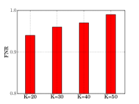
(a) Facebook

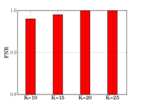
(b) Enron

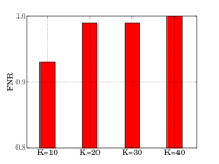
(c) Epinions

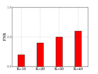
(d) Twitter

Figure 1. Impact of $K$ on our attacks on the four graphs. We observe that our attacks are more effective as $K$ increases.

Our attacks are effective and significantly outperform the baseline attacks:  Table 2 shows the results of our attacks and the baseline attacks on the four graphs for each method of selecting the target nodes and each type of cost. First, our attacks are effective. Specifically, in most scenarios, our attacks increase the FNR from 0 to be above 0.85. Moreover, our attacks are significantly more effective than the Random attack and Del-Add attack. In particular, our attacks have 0.2 to 0.6 higher FNRs than the best attack performance of the baseline attacks on the four graphs. Second, our attacks use much more inserted edges than deleted edges. A possible reason is that the graphs are sparse, i.e., only a small fraction of node pairs are connected in the original graphs. Therefore, the space of inserting edges is much larger than the space of deleting edges, leading our attacks to generate much more inserted edges. Overall, our attacks are the least effective on Facebook, i.e., our attack achieves a lowest FNR for Facebook given the same method of selecting target nodes and the same cost type. The reason is that Facebook has the largest average degree (see Table 1). With the same maximum number (i.e., $K=20$) of modified edges per node, Facebook can better tolerate our attacks.

Impact of different types of costs:  The results in Table 2 allow us to compare different types of costs. We observe that our attacks are the most effective for Equal cost and the least effective for Categorical cost. The reason is that Equal cost gives our attack the most flexibility at generating the inserted edges and deleted edges. However, for the Categorical cost scenario, it is much more expensive to modify edges between target nodes and compromised negative nodes; and it is even more expensive to modify edges between target nodes and uncompromised negative nodes. These cost constraints essentially restrict the search space of our attacks, making our attacks less effective for Categorical cost. However, we want to stress that our attacks are still effective for Categorical cost, e.g., on the Enron, Epinions, and Twitter graphs, our attacks still increase the FNR to be around 0.85. Furthermore, Table 3 shows the number of overlapped modified edges among the 3 types of costs. We observe that the number of overlapped modified edges is much smaller than the number of modified edges shown in Table 2, indicating that our attack indeed explores different search spaces for different types of costs.

Impact of different target node selection methods:  The results in Table 2 also compare RAND, CC, and CLOSE for selecting target nodes. We observe that our attacks are more effective when using CC and CLOSE than using RAND to select the target nodes, and CC and CLOSE have similar attack performance. Specifically, given the same graph and cost type, our attack achieves a higher FNR for CC and CLOSE than for RAND. For instance, with the Facebook graph and Equal cost, our attacks achieve FNRs of 0.78, 0.94, and 0.96 for RAND, CC, and CLOSE, respectively. The reason is that the target nodes selected by CC are structurally close and similar. Therefore, it is more likely for our attacks to make them evade detection “collectively”. Moreover, the target nodes selected by CLOSE are close to negative nodes and thus they are relatively easy to bypass detection. However, the target nodes selected by RAND are more structurally dissimilar; different target nodes require different efforts (inserting different edges or deleting different edges) to evade detection, and thus it is harder for our attacks to make the target nodes evade.

Table 3. Number of overlapped modified edges on different types of costs and different target node selection methods.

RAND	Equal vs. Uniform	Equal vs. Categorical	Uniform vs. Categorical
Facebook	28	0	11
Enron	94	0	12
Epinions	67	0	2
Twitter	361	17	259
CC	Equal vs. Uniform	Equal vs. Categorical	Uniform vs. Categorical
Facebook	156	72	46
Enron	176	0	9
Epinions	191	67	10
Twitter	192	40	42
CLOSE	Equal vs. Uniform	Equal vs. Categorical	Uniform vs. Categorical
Facebook	190	5	13
Enron	416	24	21
Epinions	428	260	147
Twitter	471	190	470

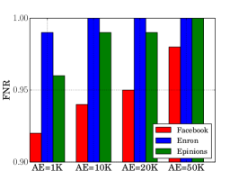
(a)

Figure 2. Impact of the number of attack edges ($AE$) on the three graphs with synthesized positive nodes for Equal cost. We observe that as $AE$ increases, FNR also increases.

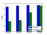
(a) Facebook

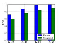
(b) Enron

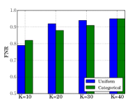
(c) Epinions

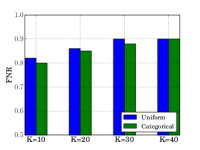
(d) Twitter

Figure 10. Impact of $K$ on the four graphs with Uniform cost and Categorical cost and with CC as the method of selecting target nodes.

Impact of $K$:  Figure 1 shows the FNRs vs. $K$ on the four graphs with Equal cost and CC as the method of selecting target nodes. The FNRs vs. $K$ with Uniform cost and Categorical cost are shown in Appendix (See Figure 10). Considering that the four graphs have different average degrees, we set different ranges of $K$ for the four graphs. We observe that as $K$ increases, FNR also increases on all the four graphs. This is because a larger $K$ allows an attacker to modify more edges per node, and thus our attacks can increase the FNRs more. Note that the total costs increase linearly as $K$, and thus we omit the results on the total cost for simplicity.

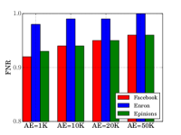
(a) Uniform cost

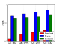
(b) Categorical cost

Figure 8. Impact of $AE$ on the three social graphs with synthesized positive nodes with (a) Uniform cost and (b) Categorical cost.

Impact of the number of attack edges (AE):  Figure 2 shows the FNRs vs. the number of attack edges on the three graphs with synthesized positive nodes for Equal cost (note that the Twitter graph has a fixed number of attack edges). The FNRs vs. $AE$ for Uniform cost and Categorical cost are shown in Appendix (See Figure 8). We observe that as $AE$ increases, our attacks achieve higher FNRs. This is because the accuracy of collective classification decreases as $AE$ increases, even without our attacks. In other words, when $AE$ is large, the FNR of the positive nodes is already large without our attacks.

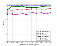
(a)

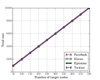
(b)

Figure 3. (a) Impact of the number of target nodes with Equal cost. We observe that FNRs are stable. (b) Costs with respect to the number of target nodes. We observe that the costs are linear to the number of target nodes.

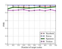
(a) Uniform cost

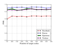
(b) Categorical cost

Figure 9. Impact of the number of target nodes on the three graphs with CC as the method of selecting target nodes. (a) Uniform cost and (b) Categorical cost.

Impact of the number of target nodes:  Figure 3a shows the FNRs vs. the number of target nodes on the four graphs, while Figure 3b shows the total cost vs. the number of target nodes, where Equal cost and CC are used. Due to the limited space, we show the FNRs vs. the number of target nodes with Uniform cost and Categorical cost in Appendix (See Figure 9). On one hand, we observe that FNRs are stable across different number of target nodes. This is because, for each target node, our attack iteratively computes the modified edges. On the other hand, our attacks require a larger total cost when the attacker uses more target nodes. Our results indicate that, our attacks can make more positive nodes evade detection when the attacker can tolerate a larger cost.

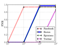
(a) $\lambda$

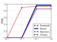
(b) $\eta$

Figure 11. Impact of $\lambda$ and $\eta$ on our attacks with Uniform cost.

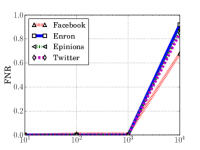
(a) $\lambda$

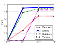
(b) $\eta$

Figure 12. Impact of $\lambda$ and $\eta$ on our attacks with Categorical cost.

Impact of hyperparameters:  Figure 4 shows the impact of $\lambda$ and $\eta$ on our attacks in the four graphs with Equal cost, where the curves for Enron and Epinions overlap. The impact of $\lambda$ and $\eta$ on our attacks with Uniform cost and Categorical cost are reported in Appendix (See Figure 11 and Figure 12). We observe phase transition phenomena for both $\lambda$ and $\eta$. Specifically, when $\lambda$ and $\eta$ are larger than certain thresholds (e.g., 100 for $\lambda$ and 0.01 for $\eta$ on Facebook), our attacks become effective. However, our attacks are less effective or ineffective when $\lambda$ and $\eta$ are smaller than the thresholds. Moreover, once $\lambda$ and $\eta$ are larger than the thresholds, our attacks are insensitive to them, e.g., the FNRs are stable. Facebook has smaller thresholds, and we speculate the reason is that Facebook is much denser than the other three graphs.

5.3. Evaluation with Partial Knowledge

We consider multiple cases where the attacker does not have access to the parameters of LinLBP, the training dataset, and/or the complete graph. We only show results on the Epinions graph as we observe similar patterns on the other three graphs, and the results for the other three graphs are shown in Appendix. Our results show that our attacks can still effectively increase the FNRs for the target nodes even if the attacker does not have access to the parameters of LinLBP, the training dataset, and/or the complete graph.

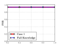
(a) $\theta$

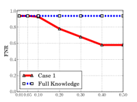
(b) $w$

Figure 13. FNRs of our attacks with different substitute parameters of LinLBP on Facebook with Equal cost.

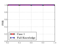
(a) $\theta$

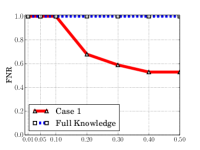
(b) $w$

Figure 14. FNRs of our attacks with different substitute parameters of LinLBP on Enron with Equal cost.

Parameter=No, Training=Yes, Graph=Complete (Case 1): In this case, the attacker does not know the parameters (i.e., $\theta$ and $w$) of LinLBP. The attacker randomly samples numbers from their corresponding domains (i.e., $0<\theta\leq 1$, $0<w\leq 0.5$) as the substitute parameters and apply our attacks with them. Figure 5 shows the FNRs of our attacks with different substitute parameters on Epinions, where $w=0.01$ when exploring different $\theta$ in Figure 5a and $\theta=0.5$ when exploring different $w$ in Figure 5b. The FNRs of our attacks with different substitute parameters on Facebook, Enron, and Twitter are shown in Figure 13, Figure 14, and Figuer 15 in Appendix, respectively. We observe that our attacks are insensitive to $\theta$. Moreover, our attacks are more effective when the substitute weight parameter is closer to the true weight. Specifically, the true weight is 0.01. Our attacks achieve FNRs that are close to 1 when the substitute weight is around 0.01, and FNRs decrease as the substitute weight increases. However, even if the substitute weight is far from the true weight, our attacks are still effective. For instance, the FNR is still 0.88 when our attack uses 0.5 as the substitute weight.

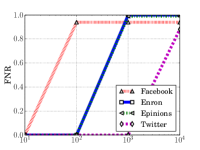
(a) $\lambda$

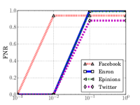
(b) $\eta$

Figure 4. Impact of $\lambda$ and $\eta$ on our attacks. We observe that our attacks achieve stable FNRs when $\lambda$ and $\eta$ are larger than certain thresholds.

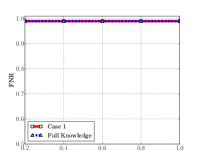
(a) $\theta$

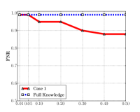
(b) $w$

Figure 5. FNRs of our attacks with different substitute parameters of LinLBP on Epinions.

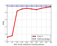
(a)

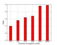
(b)

Figure 6. (a) FNRs vs. size of the substitute training dataset on Epinions; (b) FNRs when the attacker knows $\tau$% of the negative nodes and edges between them on Epinions.

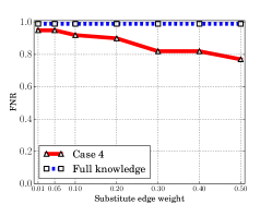
(a)

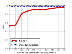
(b)

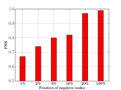
(c)

Figure 7. FNRs of our attacks vs. (a) substitute edge weight; (b) size of the substitute training dataset; (c) fraction of negative nodes on Epinions when the attacker uses substitute parameters, substitute training dataset, and a partial graph.

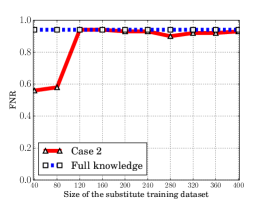
(a) Facebook

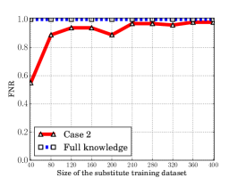
(b) Enron

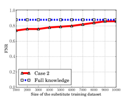
(c) Twitter

Figure 16. FNRs of our attacks vs. size of the substitute training dataset on (a) Facebook, (b) Enron, and (c) Twitter with Equal cost.

Parameter=Yes, Training=No, Graph=Complete (Case 2): In this case, the attacker does not know the true training dataset used by LinLBP. However, the attacker knows the positive nodes as they were created by itself and the negative nodes as well. Therefore, the attacker can sample some positive nodes as labeled positive nodes and sample equal number of negative nodes as labeled negative nodes, which are used as a substitute training dataset. Then, the attacker applies our attack using the substitute training dataset. Figure 6a shows the FNRs as a function of the size of the substitute training dataset on the Epinions graph. The FNRs vs. size of the substitute training dataset on Facebook, Enron, and Twitter are displayed in Figure 16a,  16b, and 16c in Appendix, respectively. We observe that as the size of the substitute training dataset increases, the FNRs of our attacks first increase dramatically and then increase slowly until reaching to the FNRs in the full knowledge scenario.

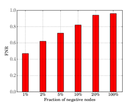
(a) Facebook

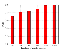
(b) Enron

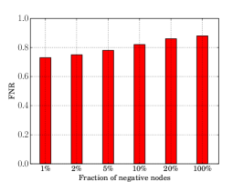
(c) Twitter

Figure 17. FNRs of our attacks on (a) Facebook, (b) Enron, and (c) Twitter with Equal cost when the attacker knows $\tau$% of the negative nodes and edges between them.

Parameter=Yes, Training=Yes, Graph=Partial (Case 3): In this scenario, the attacker knows the subgraph of positive nodes and their edges as well as a connected subgraph of some negative nodes and edges between them. Specifically, we consider the attacker knows $\tau\%$ of the negative nodes. In particular, we randomly select a negative node and span a connected component that includes $\tau\%$ of the negative nodes via breadth first search. Then, the attacker’s partial graph consists of the connected component of negative nodes, positive nodes, and the edges between them. The attacker applies our attacks using this partial graph to generate the inserted/deleted edges. Note that LinLBP still detects positive nodes using the original complete graph with the edges modified by our attacks. Figure 6b shows the FNRs of our attacks as the attacker knows a larger subgraph of negative nodes (i.e., $\tau$% is larger) on Epinions. The FNRs vs. $\tau\%$ of negative nodes on Facebook, Enron, and Twitter are shown in Figure 17a,  17b, and 17c in Appendix, respectively. We observe that as $\tau$ increases, our attacks are more effective. Moreover, when the attacker only knows $20\%$ of negative nodes, our attacks can obtain FNRs close to those when the attacker knows the complete graph.

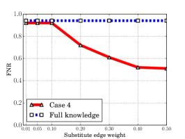
(a)

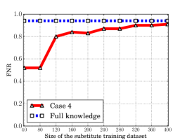
(b)

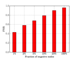
(c)

Figure 18. FNRs of our attacks vs. (a) the substitute edge weight; (b) size of the substitute training dataset; (c) fraction of negative nodes on Facebook when the attacker uses substitute parameters, substitute training dataset, and a partial graph.

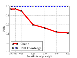
(a)

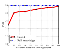
(b)

(c)

Figure 19. FNRs of our attacks vs. (a) the substitute edge weight; (b) size of the substitute training dataset; (c) fraction of negative nodes on Enron when the attacker uses substitute parameters, substitute training dataset, and a partial graph.

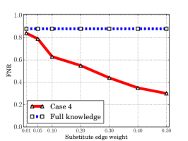
(a)

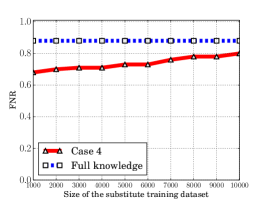
(b)

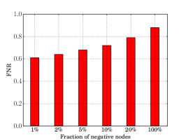
(c)

Figure 20. FNRs of our attacks vs. (a) the substitute edge weight; (b) size of the substitute training dataset; (c) fraction of negative nodes on Twitter when the attacker uses substitute parameters, substitute training dataset, and a partial graph.

Parameter=No, Training=No, Graph=Partial (Case 4):  In this case, the attacker knows the least knowledge of the three dimensions of a LinLBP system. To study our attacks in this case, we fix two dimensions and observe FNR vs. the third dimension. By default, we assume the attacker knows 20% of negative nodes and edges between them, samples a substitute training dataset with 400 nodes on Facebook, Enron, and Epinions and 3,000 nodes on Twitter, and has a substitute edge weight 0.05. Figure 7 shows FNRs of our attacks on Epinions vs. each dimension. Figure 18, Figure 19, and Figure 20 in Appendix show FNRs vs. each dimension on Facebook, Enron, and Twitter, respectively. We observe similar patterns as in Case 1, Case 2, and Case 3 (see Figure 5, Figure 6a, and Figure 6b), respectively. The reason is that our attacks do not require the true parameters, the true training dataset, nor the complete graph.

Table 4. Transferability of our attacks to other graph-based classification methods on Facebook.

RAND
Method		No attack	Equal	Uniform	Categorical
Collective Classification	LinLBP	0	0.78	0.66	0.6
	JWP	0	0.76	0.63	0.59
	LBP	0.07	0.7	0.65	0.6
	RW	0.13	0.68	0.61	0.55
Graph Neural Network	LINE	0.07	0.61	0.61	0.45
	DeepWalk	0.25	0.55	0.52	0.52
	node2vec	0.2	0.5	0.45	0.45
	GCN	0.12	0.52	0.52	0.41
CC
Method		No attack	Equal	Uniform	Categorical
Collective Classification	LinLBP	0	0.94	0.94	0.68
	JWP	0	0.93	0.93	0.63
	LBP	0.01	0.92	0.92	0.64
	RW	0.03	0.92	0.92	0.63
Graph Neural Network	LINE	0.01	0.85	0.75	0.62
	DeepWalk	0.04	0.71	0.65	0.45
	node2vec	0.04	0.69	0.61	0.45
	GCN	0.05	0.54	0.53	0.45
CLOSE
Method		No attack	Equal	Uniform	Categorical
Collective Classification	LinLBP	0	0.96	0.93	0.69
	JWP	0	0.94	0.93	0.65
	LBP	0.01	0.94	0.92	0.64
	RW	0.04	0.93	0.92	0.63
Graph Neural Network	LINE	0.01	0.86	0.77	0.59
	DeepWalk	0.05	0.72	0.69	0.48
	node2vec	0.05	0.77	0.69	0.50
	GCN	0.05	0.54	0.53	0.42

5.4. Transferring to Other Graph-based Classification Methods

Our attacks generate inserted/deleted edges based on LinLBP method. A natural question is: are our inserted/deleted edges also effective for other graph-based classification methods? To answer this question, we use our attacks to generate the modified edges based on LinLBP, modify the graph structure accordingly, and apply another graph-based classification method to detect the target nodes. Recall that graph-based classification methods can be roughly categorized as collective classification and graph neural network. We consider three representative collective classification methods, i.e., JWP (Wang et al., 2019), LBP (Gong et al., 2014a), and RW (Wang et al., 2018a), and four representative graph neural network methods, i.e., LINE (Tang et al., 2015), DeepWalk (Perozzi et al., 2014), node2vec (Grover and Leskovec, 2016), and GCN (Kipf and Welling, 2017). We obtained source code of all these methods from their corresponding authors.

Table 4 shows the effectiveness of our attacks at attacking the considered graph-based classification methods on Facebook. The results on Enron, Epinions, and Twitter are shown in Table 8, Table 9, and Table 10 in Appendix, respectively. We make several observations. First, our attacks are the most effective when using LinLBP to detect the target nodes. Specifically, when using the same method to select the target nodes and same cost type, our attacks achieve the largest FNR for the target nodes when the detector uses LinLBP. This is reasonable because our attacks generate the modified edges based on LinLBP. Second, our attacks can transfer to other graph-based classification methods, though the transferability varies among different graph-based classification methods. Third, our attacks can better transfer to other collective classification methods than other graph neural network methods in most cases. For instance, with Equal cost and CC, our attacks achieve $\geq 0.92$ FNRs for collective classification methods, while our attacks achieve 0.85 and 0.54 FNRs for LINE and GCN, respectively. The reason is collective classification methods and graph neural network methods use different mechanisms to leverage the graph structure. Fourth, our attacks have the least transferability to GCN, i.e., our attacks achieve the smallest FNRs for GCN. We speculate the reason is that GCN uses sophisticated graph convolution to exploit the higher order correlations in the graph structure, and thus is more robust to the modified edges our attacks generate.

5.5. Comparing with State-Of-The-Art Attack

We compare our attacks with state-of-the-art attack called Nettack (Zügner et al., 2018) designed for GCN.

Nettack (Zügner et al., 2018):  Nettack was designed to attack GCN (Kipf and Welling, 2017). Nettack trains a surrogate linear model of GCN. Then, Nettack defines a graph structure preserving perturbation, which constrains that the node degree distribution of the graph before and after attack should be similar. Nettack has two versions. One version only modifies the graph structure, and the other version also modifies the node attributes when they are available. We adopt the first version that modifies the graph structure. We obtained the publicly available source code of Nettack from the authors. Note that Nettack assumes Equal cost for modifying connection states between nodes.

Our attack:  It is designed based on LinLBP. We also assume Equal cost to provide a fair comparison with Nettack.

Table 5. Comparing FNRs of our attack and Nettack for different graph-based classification methods on Facebook.

Method	GCN	LINE	RW	LBP	JWP	LinLBP	Time
No attack	0.05	0.01	0.03	0.01	0	0	0 sec
Nettack	0.64	0.58	0.33	0.28	0.13	0.22	9 hrs
Our attack	0.54	0.85	0.92	0.92	0.93	0.94	10 secs

Table 5 shows the FNRs and runtime of each attack for attacking/transferring to different graph-based classification methods on Facebook, where the target nodes are selected by CC. Note that, as LINE outperforms DeepWalk and node2vec without attacks (see Table 4), we only show the transferability results of these attacks to LINE for conciseness. We only show results on Facebook, because Nettack is not scalable to the other three graphs. We note that the compared attacks have the same costs, e.g., they all modify $K$ edge states for each target node. We have several observations.

First, for attacking GCN, Nettack is the most effective, i.e., Nettack achieves the highest FNR for attacking GCN. This is because Nettack is specifically designed for GCN. Our attack can effectively transfer to GCN, though our attack is slightly less effective than Nettack at attacking GCN (0.54 vs. 0.64). Second, for attacking collective classification methods, i.e., RW, LBP, JWP, and LinLBP, our attack is much more effective than Nettack. Specifically, for all collective classification methods, our attack achieves FNRs above 0.90. However, Nettack only achieves FNRs $\leq 0.33$. The reason is that our attack is specifically designed for LinLBP and can well transfer to other collective classification methods. Third, for attacking LINE, our attack is more effective than Nettack. Specifically, our attack achieves a FNR of 0.85, while Nettack achieves a FNR of 0.58. Fourth, our attack is orders of magnitude faster than Nettack.

6. Discussion and Limitations

Attacks to other graph-based classification methods:  In this paper, we focus on designing attacks against LinLBP. The reason is that LinLBP assigns the same weight to all edges, making our formulated optimization problem easier to solve. In RW-based methods and JWP, the edge weights or propagation depend on the graph structure. Therefore, it is harder to optimize the adversarial matrix, because the gradient of the adversarial matrix also depends on the edge weights, which are implicit functions of the adversarial matrix. However, it is an interesting future work to study specialized attacks for RW-based methods and JWP.

Table 6. FPRs of our attacks on the three graphs with synthesized positive nodes for Equal cost.

Dataset	No attack	RAND	CC	CLOSE
Facebook	0.01	0.09	0.11	0.11
Enron	0.01	0.04	0.03	0.03
Epinions	0	0.10	0.10	0.10

Unavailability attacks:  In this paper, we focus on evasion attack that aims to increase the FNR of an attacker’s target nodes. In practice, an attacker could also launch the unavailability attacks. In particular, the attacker manipulates the graph structure to achieve a high False Positive Rate (FPR). A high FPR means a large amount of negative nodes are falsely classified as positive, which eventually makes the system unavailable and abandoned. We note that although our attacks are specially designed to increase the FNR of attacker’s target nodes, our attacks can also (slightly) increase the FPR. Table 6 shows the FPRs of our attacks on the three graphs with synthesized positive nodes. However, it is still an interesting future work to design attacks to specifically increase the FPR.

Poisoning training dataset:  Our work focuses on manipulating the graph structure to attack graph-based classification methods. An attacker could also poison the training dataset to attack graph-based classification methods. Specifically, in some applications, the training dataset is dynamically updated and obtained via crowdsourcing. For instance, in fraudulent user detection on social networks, a user could report other users as fraudulent users. Thus, an attacker could flag normal users as fraudster, which poison the training dataset. It is an interesting future work to poison the training dataset and compare the robustness of different graph-based classification methods against training dataset poisoning attacks.

Countermeasures:  Our work focuses on attacks to graph-based classification methods. We discuss two possible directions for defenses, and leave detailed exploration of these defenses as future work. These defense ideas are inspired by existing defenses against adversarial examples (e.g., (Goodfellow et al., 2014; Papernot et al., 2016b; Meng and Chen, 2017)) and data poisoning attacks (e.g., (Barreno et al., 2010; Jagielski et al., 2018b; Suciu et al., 2018)). Generally speaking, we could prevent and/or detect our attacks. In the prevention direction, we could explore new graph-based classification methods that are more robust to graph structure manipulation by design. In the detection direction, we could design methods to detect the inserted fake edges and deleted edges. For instance, we could extract features for each node pair and train a binary classifier, which predicts whether the connection state between the node pair was modified or not. However, when designing such a detection method, we should also consider an adaptive attacker who strategically adjusts its attacks to evade both a graph-based classification method and the detector.

Moreover, an attacker could also analyze the local structure of nodes to detect positive nodes. In particular, our attacks may change the local structure of positive nodes after inserting/deleting edges for them. For example, Table 7 shows the average clustering coefficients of the target nodes before and after our attacks on the three social graphs with synthesized positive nodes with Equal cost. We observe that the clustering coefficients slightly decrease after our attacks. This is because our attacks add neighbors to a target node, but these neighbors may not be connected. It is an interesting future work to explore the feasibility of such local structures to detect positive nodes and our attacks.

Table 7. Average clustering coefficients of target nodes before and after our attacks on the three graphs with synthesized positive nodes for Equal cost.

Dataset	RAND	CC	CLOSE
Facebook	0.492/0.464	0.540/0.492	0.591/0.573
Enron	0.567/0.549	0.634/0.632	0.559/0.554
Epinions	0.433/0.417	0.511/0.497	0.473/0.472

Attacks to graph-level classification methods:  In this paper, our attacks focus on evading node-level classification methods. In practice, graph-level classification methods have also been used for security analytics. For example, several approaches (Cesare and Xiang, 2010; Gascon et al., 2013) proposed to analyze and classify control-flow graphs for malware detection. These approaches typically make predictions on the level of graphs and hence our attacks are not applicable. We acknowledge that it is an interesting future work to design attacks against graph-level classification methods.

7. Conclusion and Future Work

We perform the first systematic study on attacks to collective classification methods via manipulating the graph structure. We propose a threat model to characterize the attack surface of collective classification methods, e.g., an attacker’s background knowledge can be characterized along the Parameter, Training dataset, and Graph dimensions. We show that our attack can be formulated as an optimization problem, which can be solved approximately by the techniques we propose. Our evaluation results on a large-scale Twitter graph with real positive nodes and three graphs with synthesized positive nodes show that our attacks can make collective classification methods misclassify an attacker’s target nodes; our attacks can transfer to graph neural network methods; our attacks do not require access to the true parameters of LinLBP, the true training dataset, and/or the complete graph; and our attacks outperform existing attacks for attacking collective classification methods and certain graph neural network methods.

Interesting future work includes 1) designing specialized attacks to other graph-based classification methods, 2) adjusting our attacks as unavailability attacks, 3) designing training data poisoning attacks to graph-based classification methods, 4) designing attacks against graph-level classification methods, and 5) enhancing robustness of graph-based classification methods.

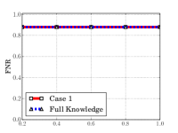
(a) $\theta$

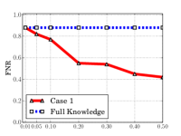
(b) $w$

Figure 15. FNRs of our attacks with different substitute parameters of LinLBP on Twitter with Equal cost.

Table 8. Transferability of our attacks to other graph-based classification methods on Enron.

RAND
Method		No attack	Equal	Uniform	Categorical
Collective Classification	LinLBP	0	1.00	0.96	0.89
	JWP	0	0.97	0.96	0.86
	LBP	0.02	0.96	0.96	0.89
	RW	0.05	0.95	0.95	0.89
Graph Neural Network	LINE	0.06	0.94	0.92	0.85
	DeepWalk	0.25	0.6	0.58	0.5
	node2vec	0.23	0.6	0.59	0.5
	GCN	0.22	0.49	0.49	0.45
CC
Method		No attack	Equal	Uniform	Categorical
Collective Classification	LinLBP	0	1.00	0.99	0.92
	JWP	0	1.00	0.98	0.89
	LBP	0	1.00	0.91	0.85
	RW	0.04	1.00	0.97	0.81
Graph Neural Network	LINE	0.04	0.98	0.95	0.63
	DeepWalk	0.23	0.7	0.65	0.45
	node2vec	0.25	0.68	0.6	0.5
	GCN	0.28	0.58	0.58	0.52
CLOSE
Method		No attack	Equal	Uniform	Categorical
Collective Classification	LinLBP	0	1.00	1.00	0.90
	JWP	0	1.00	0.99	0.90
	LBP	0	1.00	0.99	0.84
	RW	0	0.98	0.97	0.81
Graph Neural Network	LINE	0.13	1.00	0.95	0.6
	DeepWalk	0.3	1.00	0.93	0.48
	node2vec	0.30	0.95	0.89	0.50
	GCN	0.3	0.65	0.65	0.45

Table 9. Transferability of our attacks to other graph-based classification methods on Epinions. ”–” means that the method cannot be executed on our machine due to the insufficient memory.

RAND
Method		No attack	Equal	Uniform	Categorical
Collective Classification	LinLBP	0	0.98	0.94	0.92
	JWP	0	0.96	0.94	0.83
	LBP	0.07	0.96	0.94	0.92
	RW	0.08	0.95	0.87	0.9
Graph Neural Network	LINE	0.33	0.96	0.95	0.92
	DeepWalk	0.5	0.65	0.85	0.68
	node2vec	0.48	0.65	0.82	0.65
	GCN	–	–	–	–
CC
Method		No attack	Equal	Uniform	Categorical
Collective Classification	LinLBP	0	0.99	0.94	0.88
	JWP	0	0.96	0.94	0.78
	LBP	0	0.95	0.91	0.86
	RW	0	0.94	0.87	0.76
Graph Neural Network	LINE	0.31	0.96	0.9	0.86
	DeepWalk	0.45	0.75	0.78	0.68
	node2vec	0.42	0.75	0.75	0.7
	GCN	–	–	–	–
CLOSE
Method		No attack	Equal	Uniform	Categorical
Collective Classification	LinLBP	0	1.00	0.96	0.86
	JWP	0	1.00	0.96	0.86
	LBP	0	1.00	0.94	0.85
	RW	0	1.00	0.95	0.8
Graph Neural Network	LINE	0.39	0.96	0.69	0.76
	DeepWalk	0.45	0.58	0.55	0.46
	node2vec	0.42	0.59	0.59	0.49
	GCN	–	–	–	–

Table 10. Transferability of our attacks to other graph-based classification methods on Twitter.

RAND
Method		No attack	Equal	Uniform	Categorical
Collective Classification	LinLBP	0	0.85	0.85	0.82
	JWP	0	0.82	0.81	0.76
	LBP	0.01	0.82	0.8	0.72
	RW	0.03	0.78	0.77	0.69
Graph Neural Network	LINE	–	–	–	–
	DeepWalk	–	–	–	–
	node2vec	–	–	–	–
	GCN	–	–	–	–
CC
Method		No attack	Equal	Uniform	Categorical
Collective Classification	LinLBP	0	0.88	0.86	0.85
	JWP	0	0.82	0.82	0.80
	LBP	0	0.81	0.81	0.78
	RW	0.03	0.80	0.80	0.76
Graph Neural Network	LINE	–	–	–	–
	DeepWalk	–	–	–	–
	node2vec	–	–	–	–
	GCN	–	–	–	–
CLOSE
Method		No attack	Equal	Uniform	Categorical
Collective Classification	LinLBP	0	0.87	0.85	0.83
	JWP	0	0.87	0.85	0.83
	LBP	0	0.82	0.82	0.8
	RW	0.01	0.82	0.81	0.78
Graph Neural Network	LINE	–	–	–	–
	DeepWalk	–	–	–	–
	node2vec	–	–	–	–
	GCN	–	–	–	–

References

- (1)
- Akoglu et al. (2013) Leman Akoglu, Rishi Chandy, and Christos Faloutsos. 2013. Opinion Fraud Detection in Online Reviews by Network Effects.. In ICWSM.
- Alvisi et al. (2013) Lorenzo Alvisi, Allen Clement, Alessandro Epasto, Silvio Lattanzi, and Alessandro Panconesi. 2013. SoK: The Evolution of Sybil Defense via Social Networks. In IEEE S & P.
- Ateniese et al. (2015) Giuseppe Ateniese, Luigi V Mancini, Angelo Spognardi, Antonio Villani, Domenico Vitali, and Giovanni Felici. 2015. Hacking smart machines with smarter ones: How to extract meaningful data from machine learning classifiers. IJSN (2015).
- Barreno et al. (2010) Marco Barreno, Blaine Nelson, Anthony D Joseph, and JD Tygar. 2010. The security of machine learning. Machine Learning (2010).
- Battaglia et al. (2018) Peter W Battaglia, Jessica B Hamrick, Victor Bapst, Alvaro Sanchez-Gonzalez, Vinicius Zambaldi, Mateusz Malinowski, Andrea Tacchetti, David Raposo, Adam Santoro, Ryan Faulkner, et al. 2018. Relational inductive biases, deep learning, and graph networks. arXiv (2018).
- Biggio et al. (2013) Battista Biggio, Igino Corona, Davide Maiorca, Blaine Nelson, Nedim Šrndić, Pavel Laskov, Giorgio Giacinto, and Fabio Roli. 2013. Evasion attacks against machine learning at test time. In ECML-PKDD. Springer.
- Biggio et al. (2012) Battista Biggio, Blaine Nelson, and Pavel Laskov. 2012. Poisoning attacks against support vector machines. In ICML.
- Bojchevski and Günnemann (2019) Aleksandar Bojchevski and Stephan Günnemann. 2019. Adversarial Attacks on Node Embeddings via Graph Poisoning. In ICML.
- Boshmaf et al. (2015) Yazan Boshmaf, Dionysios Logothetis, Georgos Siganos, Jorge Leria, Jose Lorenzo, Matei Ripeanu, and Konstantin Beznosov. 2015. Integro: Leveraging Victim Prediction for Robust Fake Account Detection in OSNs. In NDSS.
- Cao et al. (2012) Qiang Cao, Michael Sirivianos, Xiaowei Yang, and Tiago Pregueiro. 2012. Aiding the Detection of Fake Accounts in Large Scale Social Online Services. In NSDI.
- Cao et al. (2015) Shaosheng Cao, Wei Lu, and Qiongkai Xu. 2015. Grarep: Learning graph representations with global structural information. In CIKM.
- Carlini et al. (2016) Nicholas Carlini, Pratyush Mishra, Tavish Vaidya, Yuankai Zhang, Micah Sherr, Clay Shields, David Wagner, and Wenchao Zhou. 2016. Hidden Voice Commands. In USENIX Security Symposium.
- Cesare and Xiang (2010) Silvio Cesare and Yang Xiang. 2010. Classification of malware using structured control flow. In AusPDC. Australian Computer Society, Inc.
- Chau et al. (2011) Duen Horng “Polo” Chau, Carey Nachenberg, Jeffrey Wilhelm, Adam Wright, and Christos Faloutsos. 2011. Polonium: Tera-scale graph mining and inference for malware detection. In SIAM SDM.
- Chen et al. (2017) Yizheng Chen, Yacin Nadji, Athanasios Kountouras, Fabian Monrose, Roberto Perdisci, Manos Antonakakis, and Nikolaos Vasiloglou. 2017. Practical attacks against graph-based clustering. In CCS.
- Dai et al. (2018b) Hanjun Dai, Hui Li, Tian Tian, Xin Huang, Lin Wang, Jun Zhu, and Le Song. 2018b. Adversarial Attack on Graph Structured Data. In ICML.
- Dai et al. (2018a) Quanyu Dai, Qiang Li, Jian Tang, and Dan Wang. 2018a. Adversarial network embedding. In AAAI.
- Defferrard et al. (2016) Michaël Defferrard, Xavier Bresson, and Pierre Vandergheynst. 2016. Convolutional neural networks on graphs with fast localized spectral filtering. In NIPS.
- Fang et al. (2018) Minghong Fang, Guolei Yang, Neil Zhenqiang Gong, and Jia Liu. 2018. Poisoning Attacks to Graph-Based Recommender Systems. In ACSAC.
- Fredrikson et al. (2015) Matt Fredrikson, Somesh Jha, and Thomas Ristenpart. 2015. Model inversion attacks that exploit confidence information and basic countermeasures. In CCS.
- Fredrikson et al. (2014) Matthew Fredrikson, Eric Lantz, Somesh Jha, Simon Lin, David Page, and Thomas Ristenpart. 2014. Privacy in pharmacogenetics: An end-to-end case study of personalized warfarin dosing. In USENIX Security Symposium.
- Ganju et al. (2018) Karan Ganju, Qi Wang, Wei Yang, Carl A Gunter, and Nikita Borisov. 2018. Property Inference Attacks on Fully Connected Neural Networks using Permutation Invariant Representations. In CCS.
- Gao et al. (2018) Peng Gao, Binghui Wang, Neil Zhenqiang Gong, Sanjeev R Kulkarni, Kurt Thomas, and Prateek Mittal. 2018. SybilFuse: Combining Local Attributes with Global Structure to Perform Robust Sybil Detection. In IEEE CNS.
- Gascon et al. (2013) Hugo Gascon, Fabian Yamaguchi, Daniel Arp, and Konrad Rieck. 2013. Structural detection of android malware using embedded call graphs. In AISec.
- Gong et al. (2014a) Neil Zhenqiang Gong, Mario Frank, and Prateek Mittal. 2014a. SybilBelief: A Semi-supervised Learning Approach for Structure-based Sybil Detection. IEEE TIFS (2014).
- Gong and Liu (2016) Neil Zhenqiang Gong and Bin Liu. 2016. You are Who You Know and How You Behave: Attribute Inference Attacks via Users’ Social Friends and Behaviors. In USENIX Security Symposium.
- Gong et al. (2014b) Neil Zhenqiang Gong, Ameet Talwalkar, Lester Mackey, Ling Huang, Eui Chul Richard Shin, Emil Stefanov, Elaine Runting Shi, and Dawn Song. 2014b. Joint link prediction and attribute inference using a social-attribute network. ACM TIST (2014).
- Goodfellow et al. (2014) Ian J Goodfellow, Jonathon Shlens, and Christian Szegedy. 2014. Explaining and harnessing adversarial examples. arXiv (2014).
- Grover and Leskovec (2016) Aditya Grover and Jure Leskovec. 2016. node2vec: Scalable feature learning for networks. In KDD.
- Gyöngyi et al. (2004) Zoltán Gyöngyi, Hector Garcia-Molina, and Jan Pedersen. 2004. Combating web spam with trustrank. In VLDB.
- Huang et al. (2011) Ling Huang, Anthony D Joseph, Blaine Nelson, Benjamin IP Rubinstein, and JD Tygar. 2011. Adversarial machine learning. In AISec.
- Jagielski et al. (2018a) Matthew Jagielski, Alina Oprea, Battista Biggio, Chang Liu, Cristina Nita-Rotaru, and Bo Li. 2018a. Manipulating machine learning: Poisoning attacks and countermeasures for regression learning. In IEEE S & P.
- Jagielski et al. (2018b) Matthew Jagielski, Alina Oprea, Battista Biggio, Chang Liu, Cristina Nita-Rotaru, and Bo Li. 2018b. Manipulating Machine Learning: Poisoning Attacks and Countermeasures for Regression Learning. In IEEE S & P.
- Ji et al. (2018) Yujie Ji, Xinyang Zhang, Shouling Ji, Xiapu Luo, and Ting Wang. 2018. Model-Reuse Attacks on Deep Learning Systems. In CCS.
- Jia and Gong (2018) Jinyuan Jia and Neil Zhenqiang Gong. 2018. AttriGuard: A Practical Defense Against Attribute Inference Attacks via Adversarial Machine Learning. USENIX Security Symposium (2018).
- Jia et al. (2017a) Jinyuan Jia, Binghui Wang, and Neil Zhenqiang Gong. 2017a. Random Walk based Fake Account Detection in Online Social Networks. In IEEE DSN.
- Jia et al. (2017b) Jinyuan Jia, Binghui Wang, Le Zhang, and Neil Zhenqiang Gong. 2017b. AttriInfer: Inferring User Attributes in Online Social Networks Using Markov Random Fields. In WWW.
- Kipf and Welling (2017) Thomas N Kipf and Max Welling. 2017. Semi-supervised classification with graph convolutional networks. In ICLR.
- Li et al. (2016) Bo Li, Yining Wang, Aarti Singh, and Yevgeniy Vorobeychik. 2016. Data Poisoning Attacks on Factorization-Based Collaborative Filtering. In NIPS.
- Li et al. (2013) Zhou Li, Sumayah Alrwais, Yinglian Xie, Fang Yu, and XiaoFeng Wang. 2013. Finding the linchpins of the dark web: a study on topologically dedicated hosts on malicious web infrastructures. In IEEE S & P.
- Liu et al. (2015) Changchang Liu, Peng Gao, Matthew Wright, and Prateek Mittal. 2015. Exploiting temporal dynamics in sybil defenses. In CCS.
- Liu et al. (2017) Yanpei Liu, Xinyun Chen, Chang Liu, and Dawn Song. 2017. Delving into Transferable Adversarial Examples and Black-box Attacks. In ICLR.
- Meng and Chen (2017) Dongyu Meng and Hao Chen. 2017. MagNet: a Two-Pronged Defense against Adversarial Examples. In CCS.
- Mikolov et al. (2013) Tomas Mikolov, Ilya Sutskever, Kai Chen, Greg S Corrado, and Jeff Dean. 2013. Distributed representations of words and phrases and their compositionality. In NIPS.
- Nelson et al. (2010) Blaine Nelson, Benjamin IP Rubinstein, Ling Huang, Anthony D Joseph, Shing-hon Lau, Steven J Lee, Satish Rao, Anthony Tran, and J Doug Tygar. 2010. Near-Optimal Evasion of Convex-Inducing Classifiers.. In AISTATS.
- Oprea et al. (2015) Alina Oprea, Zhou Li, Ting-Fang Yen, Sang H Chin, and Sumayah Alrwais. 2015. Detection of early-stage enterprise infection by mining large-scale log data. In DSN.
- Pandit et al. (2007) Shashank Pandit, Duen Horng Chau, Samuel Wang, and Christos Faloutsos. 2007. Netprobe: a fast and scalable system for fraud detection in online auction networks. In WWW.
- Papernot et al. (2016a) Nicolas Papernot, Patrick McDaniel, Somesh Jha, Matt Fredrikson, Z. Berkay Celik, and Ananthram Swami. 2016a. The Limitations of Deep Learning in Adversarial Settings. In EuroS&P.
- Papernot et al. (2016b) Nicolas Papernot, Patrick McDaniel, Xi Wu, Somesh Jha, and Ananthram Swami. 2016b. Distillation as a Defense to Adversarial Perturbations against Deep Neural Networks. In IEEE S & P.
- Perozzi et al. (2014) Bryan Perozzi, Rami Al-Rfou, and Steven Skiena. 2014. Deepwalk: Online learning of social representations. In KDD.
- Pyrgelis et al. (2018) Apostolos Pyrgelis, Carmela Troncoso, and Emiliano De Cristofaro. 2018. Knock Knock, Who’s There? Membership Inference on Aggregate Location Data. In NDSS.
- Scarselli et al. (2009) Franco Scarselli, Marco Gori, Ah Chung Tsoi, Markus Hagenbuchner, and Gabriele Monfardini. 2009. The graph neural network model. IEEE TNN (2009).
- Sharif et al. (2016) Mahmood Sharif, Sruti Bhagavatula, Lujo Bauer, and K Michael Reiter. 2016. Accessorize to a Crime: Real and Stealthy Attacks on State-of-the-Art Face Recognition. In CCS.
- Shokri et al. (2017) Reza Shokri, Marco Stronati, Congzheng Song, and Vitaly Shmatikov. 2017. Membership Inference Attacks Against Machine Learning Models. In IEEE S & P.
- Srndic and Laskov (2014) Nedim Srndic and Pavel Laskov. 2014. Practical evasion of a learning-based classifier: A case study. In IEEE S & P.
- Suciu et al. (2018) Octavian Suciu, Radu Marginean, Yigitcan Kaya, Hal Daume III, and Tudor Dumitras. 2018. When Does Machine Learning FAIL? Generalized Transferability for Evasion and Poisoning Attacks. In Usenix Security Symposium.
- Sun et al. (2018) Mingjie Sun, Jian Tang, Huichen Li, Bo Li, Chaowei Xiao, Yao Chen, and Dawn Song. 2018. Data Poisoning Attack against Unsupervised Node Embedding Methods. Arxiv (2018).
- Szegedy et al. (2013) Christian Szegedy, Wojciech Zaremba, Ilya Sutskever, Joan Bruna, Dumitru Erhan, Ian Goodfellow, and Rob Fergus. 2013. Intriguing properties of neural networks. arXiv (2013).
- Tamersoy et al. (2014) Acar Tamersoy, Kevin Roundy, and Duen Horng Chau. 2014. Guilt by association: large scale malware detection by mining file-relation graphs. In KDD.
- Tang et al. (2015) Jian Tang, Meng Qu, Mingzhe Wang, Ming Zhang, Jun Yan, and Qiaozhu Mei. 2015. Line: Large-scale information network embedding. In WWW.
- Torkamani and Lowd (2013) MohamadAli Torkamani and Daniel Lowd. 2013. Convex adversarial collective classification. In ICML. 642–650.
- Tramèr et al. (2016) Florian Tramèr, Fan Zhang, Ari Juels, Michael K Reiter, and Thomas Ristenpart. 2016. Stealing machine learning models via prediction apis. In USENIX Security Symposium.
- Wang and Gong (2018) Binghui Wang and Neil Zhenqiang Gong. 2018. Stealing hyperparameters in machine learning. In IEEE S & P.
- Wang et al. (2017a) Binghui Wang, Neil Zhenqiang Gong, and Hao Fu. 2017a. GANG: Detecting Fraudulent Users in Online Social Networks via Guilt-by-Association on Directed Graphs. In IEEE ICDM.
- Wang et al. (2019) Binghui Wang, Jinyuan Jia, and Neil Zhenqiang Gong. 2019. Graph-based Security and Privacy Analytics via Collective Classification with Joint Weight Learning and Propagation. In NDSS.
- Wang et al. (2018a) Binghui Wang, Jinyuan Jia, Le Zhang, and Neil Zhenqiang Gong. 2018a. Structure-based Sybil Detection in Social Networks via Local Rule-based Propagation. IEEE TNSE (2018).
- Wang et al. (2017b) Binghui Wang, Le Zhang, and Neil Zhenqiang Gong. 2017b. SybilSCAR: Sybil Detection in Online Social Networks via Local Rule based Propagation. In IEEE INFOCOM.
- Wang et al. (2018b) Binghui Wang, Le Zhang, and Neil Zhenqiang Gong. 2018b. SybilBlind: Detecting Fake Users in Online Social Networks without Manual Labels. In RAID.
- Weston et al. (2012) Jason Weston, Frédéric Ratle, Hossein Mobahi, and Ronan Collobert. 2012. Deep learning via semi-supervised embedding. In Neural Networks: Tricks of the Trade. Springer, 639–655.
- Xiao et al. (2015) Huang Xiao, Battista Biggio, Gavin Brown, Giorgio Fumera, Claudia Eckert, and Fabio Roli. 2015. Is feature selection secure against training data poisoning?. In ICML.
- Xu et al. (2016) Weilin Xu, Yanjun Qi, and David Evans. 2016. Automatically Evading Classifiers: A Case Study on PDF Malware Classifiers. In NDSS.
- Yang et al. (2012) Chao Yang, Robert Harkreader, Jialong Zhang, Seungwon Shin, and Guofei Gu. 2012. Analyzing Spammer’s Social Networks for Fun and Profit. In WWW.
- Yang et al. (2017) Guolei Yang, Neil Zhenqiang Gong, and Ying Cai. 2017. Fake Co-visitation Injection Attacks to Recommender Systems. In NDSS.
- Yu et al. (2008) H. Yu, P. B. Gibbons, M. Kaminsky, and F. Xiao. 2008. SybilLimit: A Near-Optimal Social Network Defense against Sybil Attacks. In IEEE S & P.
- Yuan and Ghanem (2017) Ganzhao Yuan and Bernard Ghanem. 2017. An Exact Penalty Method for Binary Optimization Based on MPEC Formulation.. In AAAI.
- Zhu et al. (2003) Xiaojin Zhu, Zoubin Ghahramani, John Lafferty, et al. 2003. Semi-supervised learning using gaussian fields and harmonic functions. In ICML.
- Zügner et al. (2018) Daniel Zügner, Amir Akbarnejad, and Stephan Günnemann. 2018. Adversarial attacks on neural networks for graph data. In KDD.
- Zügner and Günnemann (2019a) Daniel Zügner and Stephan Günnemann. 2019a. Adversarial attacks on graph neural networks via meta learning. In ICLR.
- Zügner and Günnemann (2019b) Daniel Zügner and Stephan Günnemann. 2019b. Certifiable Robustness and Robust Training for Graph Convolutional Networks. In KDD. ACM.