Convenient filtering techniques for LIGO strain of the GW150914 event

Abstract

We present a new strategy for the pre-processing filtering techniques of the LIGO strain of the GW150914[1, 2] event that intends to extract as much physical information as possible, minimizing the use of prior assumptions, and avoiding transformations of the astrophysical signal.

The new techniques allow us to reveal more low frequency signal at earlier times, that it has been overlooked.

1 Introduction

Among all the gravitational waves events announced[1, 2, 3, 4, 5, 6, 7, 8, 9] by the LIGO/Virgo Collaboration, still the GW150914 event remains the one showing the strongest signal to noise ratio. It is because of this that many studies[10, 11, 12, 13, 14, 15] on gravitational waves data devote special attention to it. We are here concerned with the first manipulation on the data previous to the full study of the nature of the physical signal contained in it

In order to study the physical content of the Handford and Livingstone LIGO data for the GW150914 event, the LIGO/Virgo Collaboration has applied pre-processing filtering techniques that include whitening filter, 35–350 Hz bandpass filter and band-reject filters to remove the strong instrumental spectral lines, in [1], and in [2] they only state to have whitened the data by the noise power spectral density. In [16] the LIGO/Virgo Collaboration carried out a matched-filter search for GW150914 using relativistic models of compact-object binaries using a couple of techniques; but in both they use a low-frequency cutoff of 30 Hz for the search, and in one of them they also used whitening filter. Also in the analysis of reference [17] they report to have used whitening filters.

This article deals with the strategy for the pre-processing filtering techniques; in particular we present arguments against the use of whitening filters, and we present a set of finite impulse filters (FIR) that will show to be more convenient, for the pre-processing stage. After this then one can more safely process the data with for example matched filter searches[16].

The organization of this article is as follows. In section 2 we present a preliminary study of the nature of the data and a review of the LIGO Collaboration filtering techniques. Our suggestion for the pre-processing filtering is presented in section 3; and in section 4 we include some final comments on the work and suggest further study.

2 Preliminary view of the raw data

Before embarking in the presentation of the new filtering approach, let us review the main characteristics of the LIGO data around the event GW150914.

2.1 Spectrograms near the event

One of the main indications that something interesting happens around the time of the GW150914 event that we take it to be: $t_{e}=1126259462.422$GPS, equivalent to: Mon Sep 14 09:50:45 GMT 2015, as suggested by LIGO at first, is the study of the spectrograms that we show in figure 1. One can see that a faint almost vertical line on both spectrograms at around the time assigned to the event.

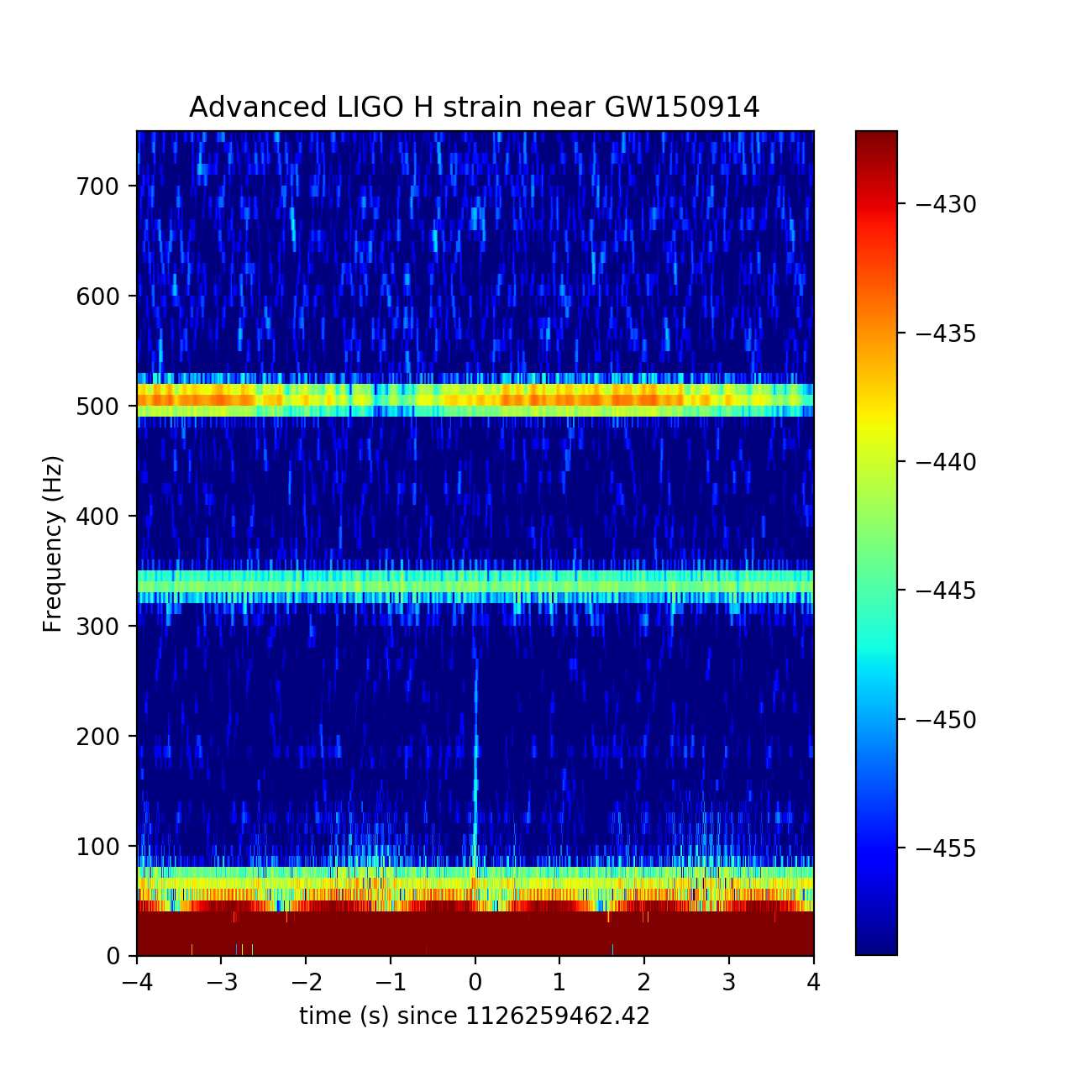
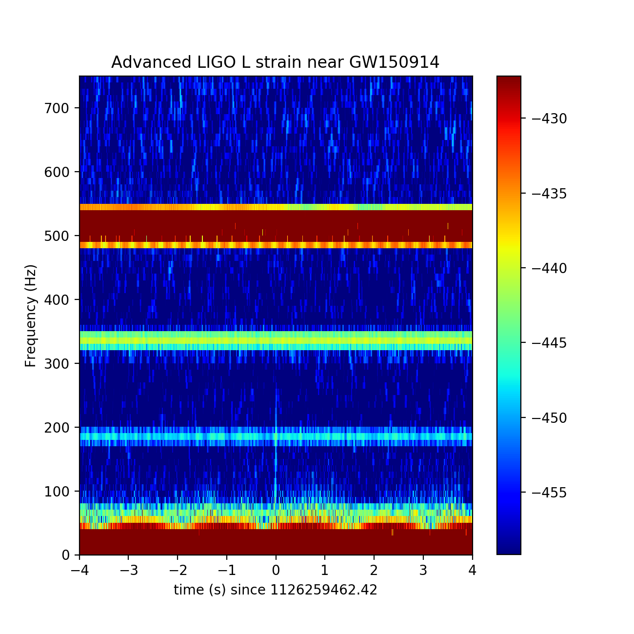
Figure 1: Spectrograms of raw data from Hanford on the left, and Livingston on the right; $\pm$4 seconds around the time of event GW150914, in the range from 0 to 750Hz.

Since the detectors are separated by about 3000km, the fact that both detectors show the same appearance of an increasing in frequency signal, with a time separation of less than 10ms indicates that this event is probably caused by an astrophysical system far from Earth.

It is worthwhile to emphasize that this preliminary study does not need for any a priori knowledge of calculated templates; since it is noticed in the raw data.

2.2 The amplitude spectral density of 256s around the event

We are concerned with the details of the intrinsic noises of the detectors; for this reason we do almost all studies with a fairly wide extension of data of length 256 seconds around the time of the event GW150914. This choice allows us to work with broader windows when performing studies and constructing filters. For example in figure 2, where we show the amplitude spectral densities (ASD) of both detectors, we also present the details of ASD in the range 34-37Hz, where calibration lines appear as very narrow peaks. These have been of concern in [12], where they have worked with a 32 seconds time lapse of data; and it can be seen that our figure 2 which compares with their figure 2, shows that these peaks are very narrow when studied with 90 seconds windows. This is important for our work since this allows for constructing narrow stopband filters to eliminate these unwanted contributions to the strain. The three graphs of figure 2 have been constructed with 90seconds windows on the 256 seconds strain.

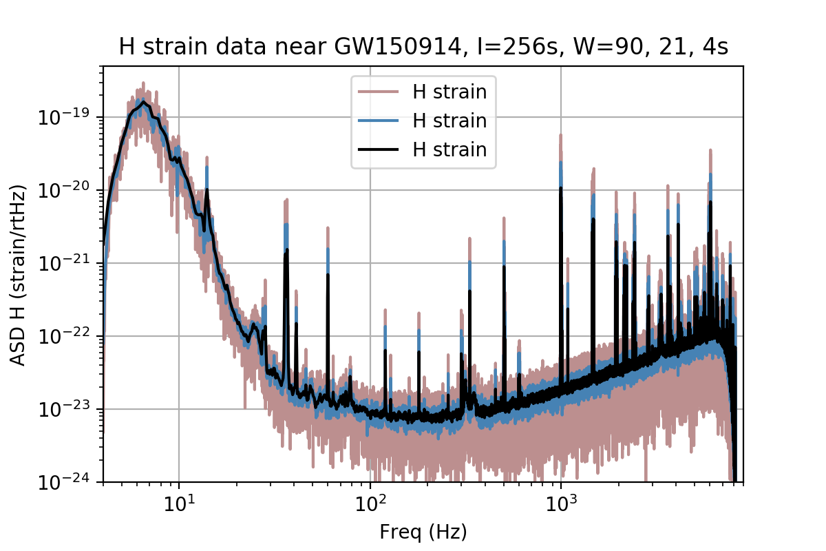
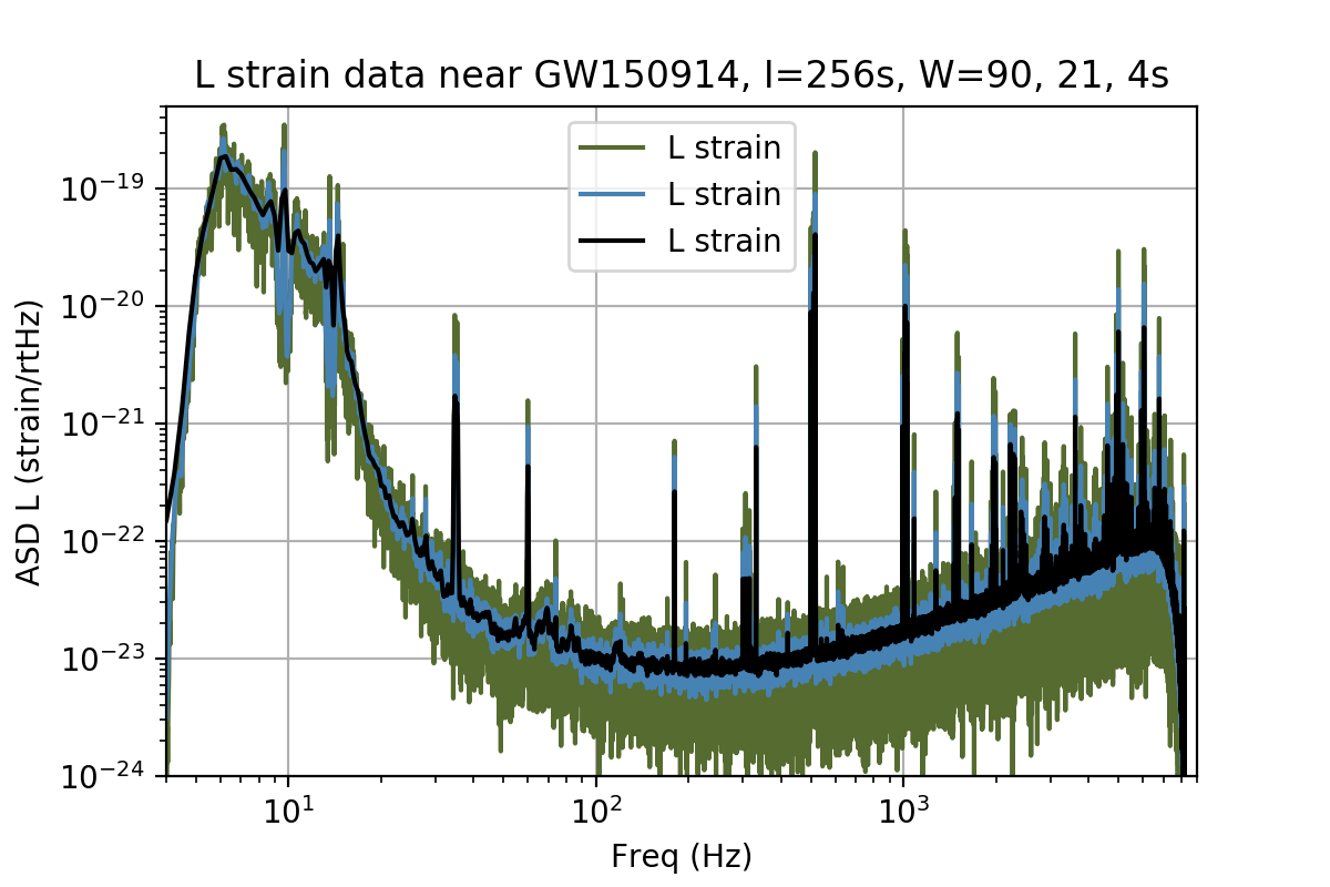
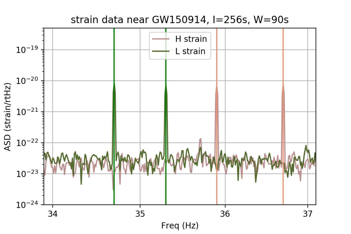
Figure 2: Amplitude spectral density of raw data from Hanford on the left, and Livingston at the center, in the range from 4 to 9000Hz, for the interval of 256s around the time of the event with 90s windows; where one can observe the cutoff at the Nyquist frequency. On the right, a detail from 34 to 37Hz from both detectors; where due to the fact that we are using a 90 seconds windows, one can see that the calibrating signals are very narrow. The vertical lines mark the frequencies 34.7Hz and 35.3Hz for Livingston, and 35.9Hz and 36.7Hz for Hanford.

In the left and center graphs we have also superimposed the amplitude spectral density of each detector using also windows of 21s and 4s. It can be seen that the 90s windows show the widest ASD; then the 21s windowsASD(in light blue) are narrower and finally the 4s windows ASD(in black) are the thinnest. This is motivating for our work since it means that when one increases the statistics, the ASD show wider variations than those calculated with short windows, since they have increasing frequency resolution.

2.3 The usual whitening procedure performed by LIGO

Details of the GW150914 data have been presented by LIGO Collaboration through the study of various filtering techniques. In figure 6 of reference [2] one can see graphs of the data, sampled at 2048Hz, where whitening filters were applied. In figure 3 we present the effects on the amplitude spectral density of 256s intervals of data, using 4s windows, and the full sampling rate of 16384Hz; where each whitening filter is normalized in order to preserve the strain amplitude at the respective minimum of the amplitude spectral density for each detector.

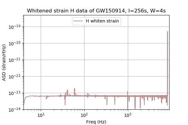
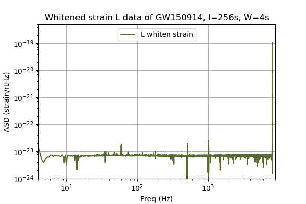
Figure 3: Amplitude spectral density of the whitened strains for 256s intervals, and windows of 4s, as suggested in LIGO public python scripts. Hanford data on the left and Livingston’s on the right.

In LIGO reference [1] they have used a 35–350Hz bandpass Butterworth filter, which we also apply to the data we are considering, according to the indications in the public LIGO python scripts. In figure 4 we show the amplitude spectral density graphs of the 256s intervals, after applying the bandbass filter, where we have used the same axis limits, in order to emphasize the effects of this filter.

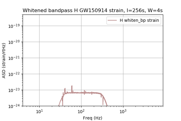
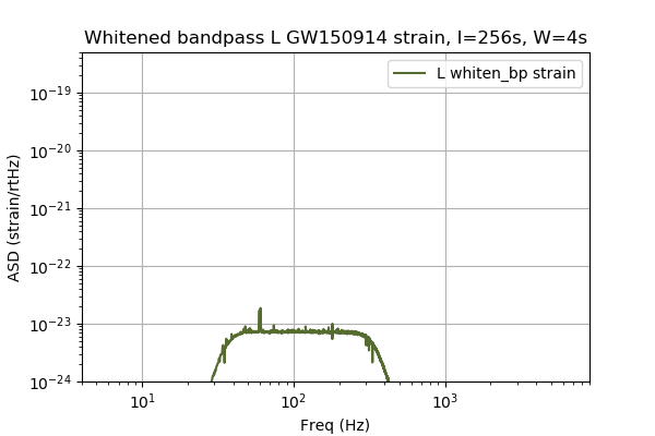
Figure 4: Amplitude spectral density of the whitened and bandpass strains for 256s intervals, and windows of 4s, as suggested in LIGO public python scripts. Hanford data on the left and Livingston’s on the right.

2.4 Phase diagrams of the raw data and after filtering

In figure 5 we show the phase diagrams of the raw data of both detectors for 256s centered at the time of the GW150914 event, up to 500Hz.

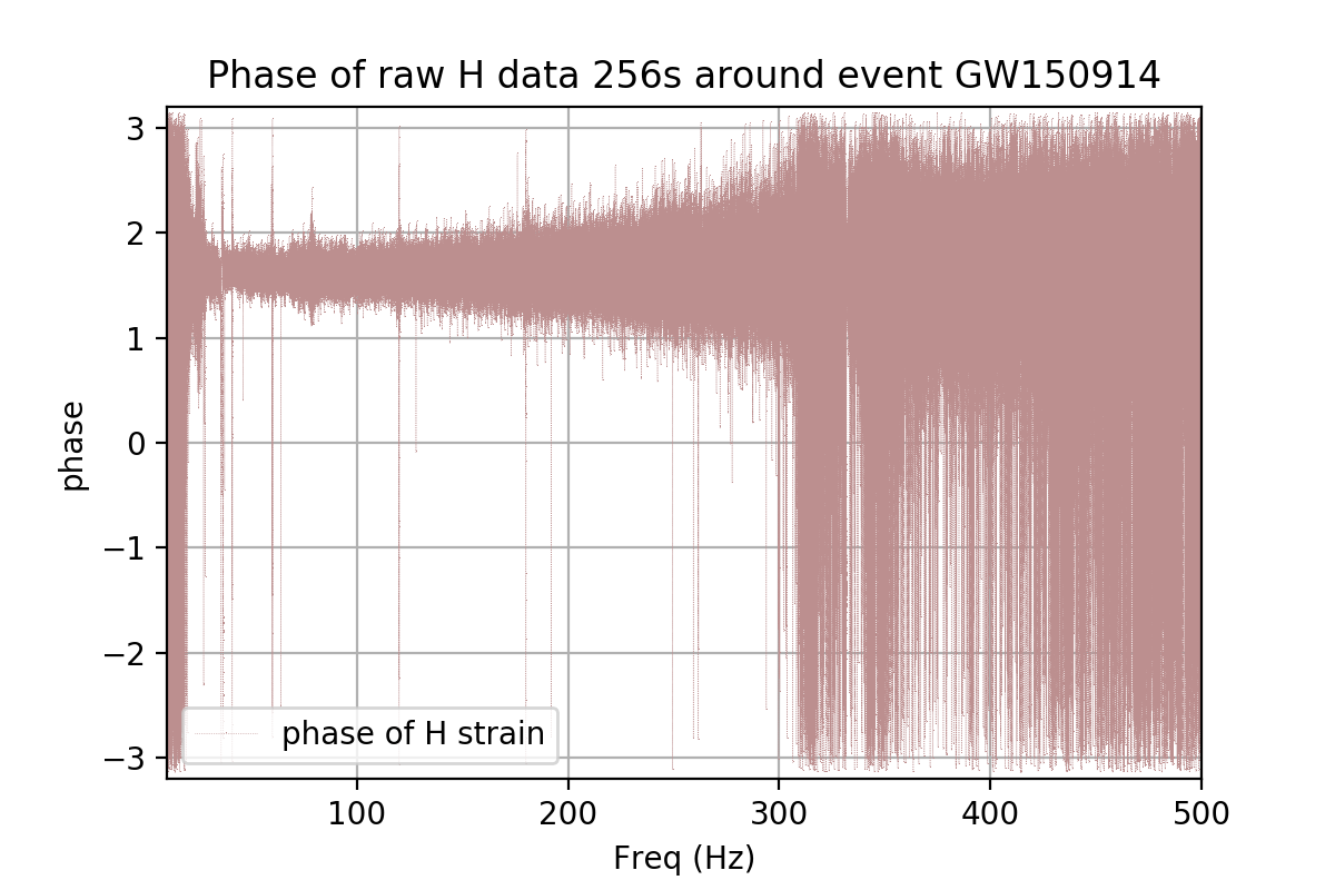
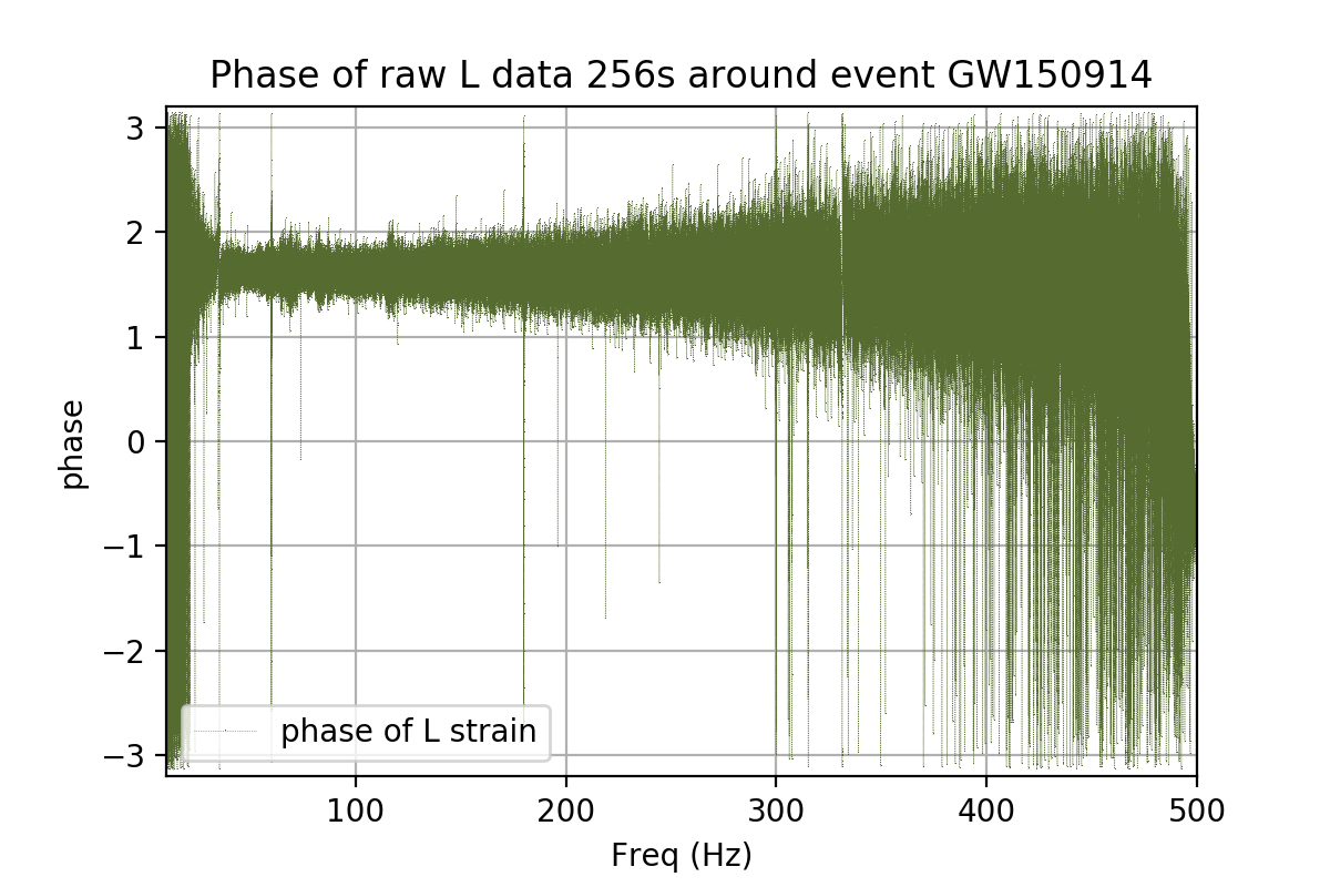
Figure 5: Phase diagrams as a function of frequency for the raw data of 256s length around the time of the event GW150914, showing Hanford on the left and Livingston on the right.

It can be noticed that they show strong correlations and since we are dealing with the full sampling rate of the data at $f_{s}=16384$Hz, and with a 256s time interval, our graphs are also different from those shown in [12]. Since these studies depend very much on the length of the time interval, and the sampling rate, this reinforces the interpretation that at this raw stage the noise is not Gaussian.

We show the phases as function of frequencies, after applying the LIGO filtering procedures, in figure 6, up to 350Hz.

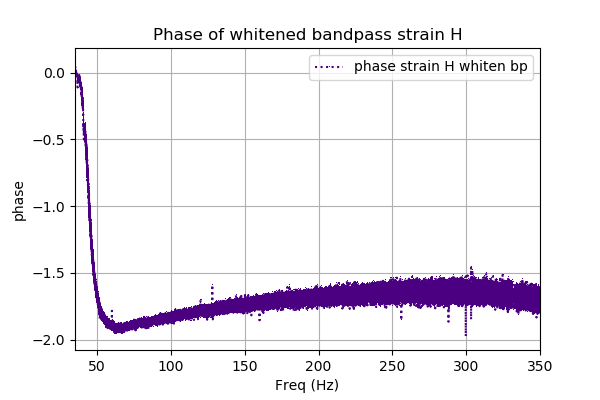
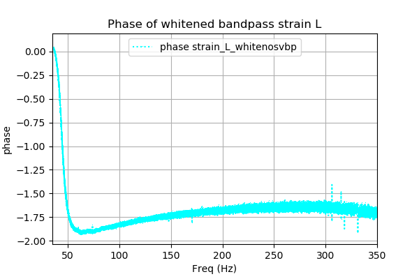
Figure 6: Phase diagrams as a function of frequency after applying the LIGO whitening and bandpass filter to the data of 256s length around the time of the event GW150914, showing Hanford on the left and Livingston on the right.

It can be seen in figure 6 that the 256s statistics results in narrower bands, than those found in the studies shown in figure 3 of reference [12]; therefore, the concerns expressed there, on the phase behavior, are augmented here.

We show these figures not to participate in a debate on the meaning of the signal at both detectors, instead, we just want to illustrate that the application of whitening and bandpass filters are to be handled with most care; since otherwise unwanted side effects involving phase behavior and group delay[18] might appear. But our main concern is related to the severe relative attenuation of low frequencies in the whitening procedure with the characteristics of LIGO amplitude spectral density of each detector, as it can be noticed below in our study of the effects of LIGO filtering on the templates.

2.5 Effects of the whitening and bandpass LIGO filtering on templates

The LIGO Scientific Collaboration has also made public the components of the waveform templates that where used in matched filtering. We follow the indications of the public LIGO python scripts to find, from both components of the calculated template, those that match for Hanford and Livingstone detectors; that below will appear as template_H and template_L in the graphs.

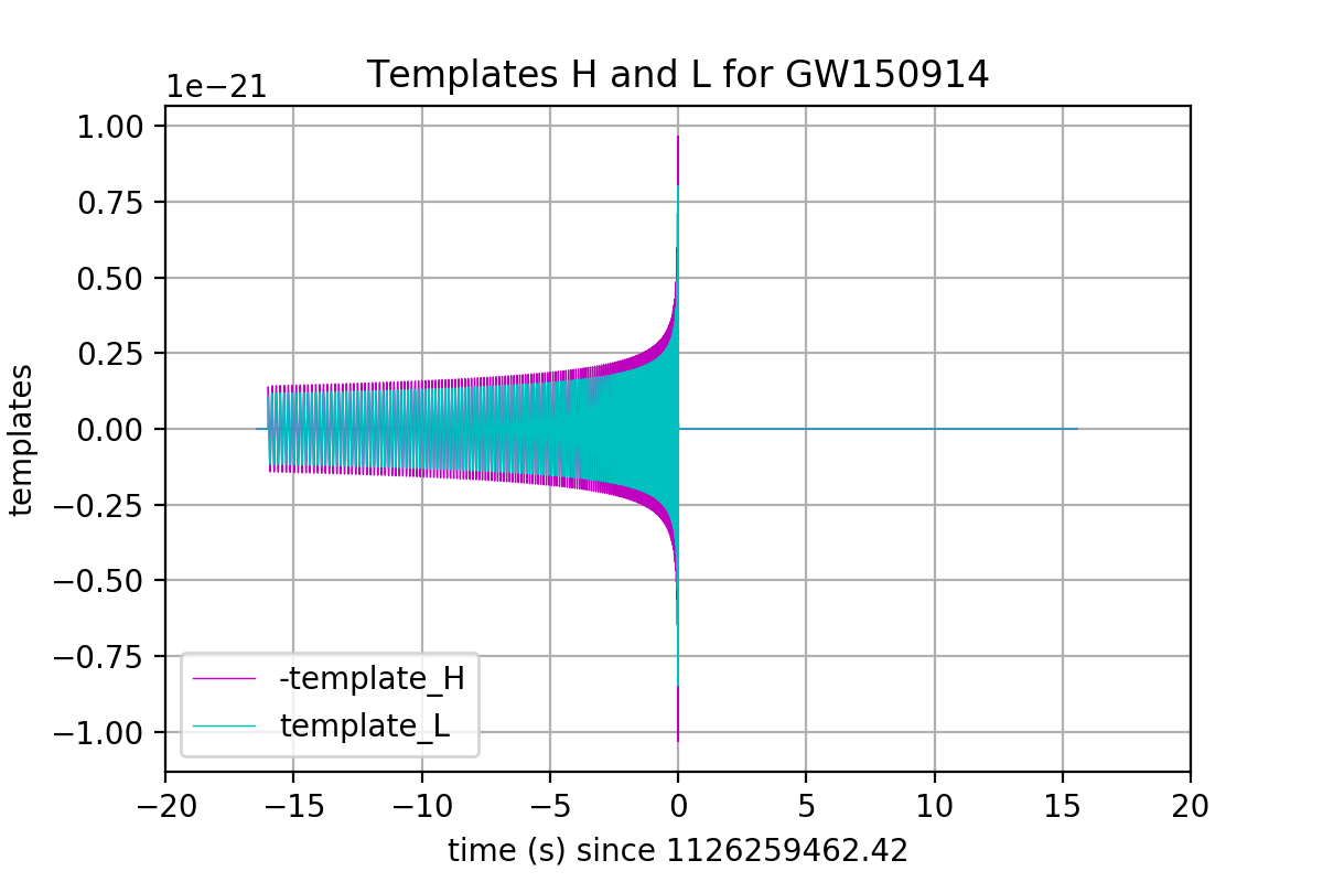
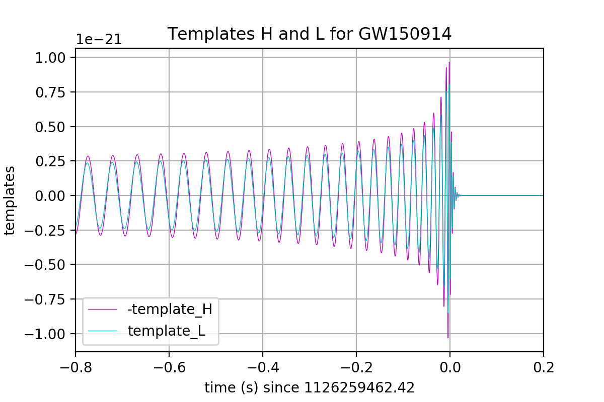
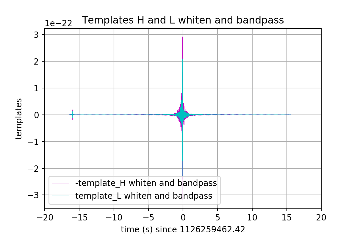
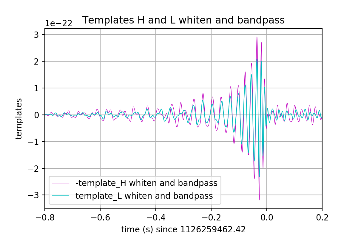
Figure 7: Matched templates for Hanford and Livingston GW150914 event. In top left graph, the full time extend of the original templates; while on the top right, the detail of 1s length around the time of the event. In the bottom row, the corresponding graphs after applying the whitening and bandpass of 35-350Hz filter.

One can see in the graphs of figure 7 that the filtering procedure suggested by LIGO, severely changes the shape of the matched templates; which are supposed to give a close representation of the expected physical signal hidden in the observed data. In particular, in the lower right graph, it is noted that by applying these filters, one can only use a very limited lapse of time in the signal, on the order of 0.1second. We will argue below against this limitation imposed by the filtering approach suggested by the LIGO Collaboration.

3 The new filtering scheme without whitening

A comparison of the U shape shown in figure 2 and the flat shape shown in 3 indicates that if there were a physical signal with frequencies below that one at minimum of the ASD; then they will be severely attenuated by the whitening procedure. We present here a new approach to the initial filtering in order to circumvent this effect.

3.1 Initial bandpass filter

It is sensible to apply an initial bandpass filter in order to concentrate on the main frequency band that might contain physically interesting signals. For this reason we choose a very wide band that goes from 22Hz to 1024Hz. However, instead of the infinite impulse response (IIR) filters used in the public LIGO python scripts, we choose to apply finite impulse response (FIR) filters; which are supposed to have safer phase behavior.

Since we are interested in an interval of 256s and the FIR bandpass filters might include boundary effects, we start with a 288s interval centered at the time of the event, and after applying the FIR bandpass filter, we crop it to an interval of 256s centered at the event time, whose resulting ASD are shown in figure 8.

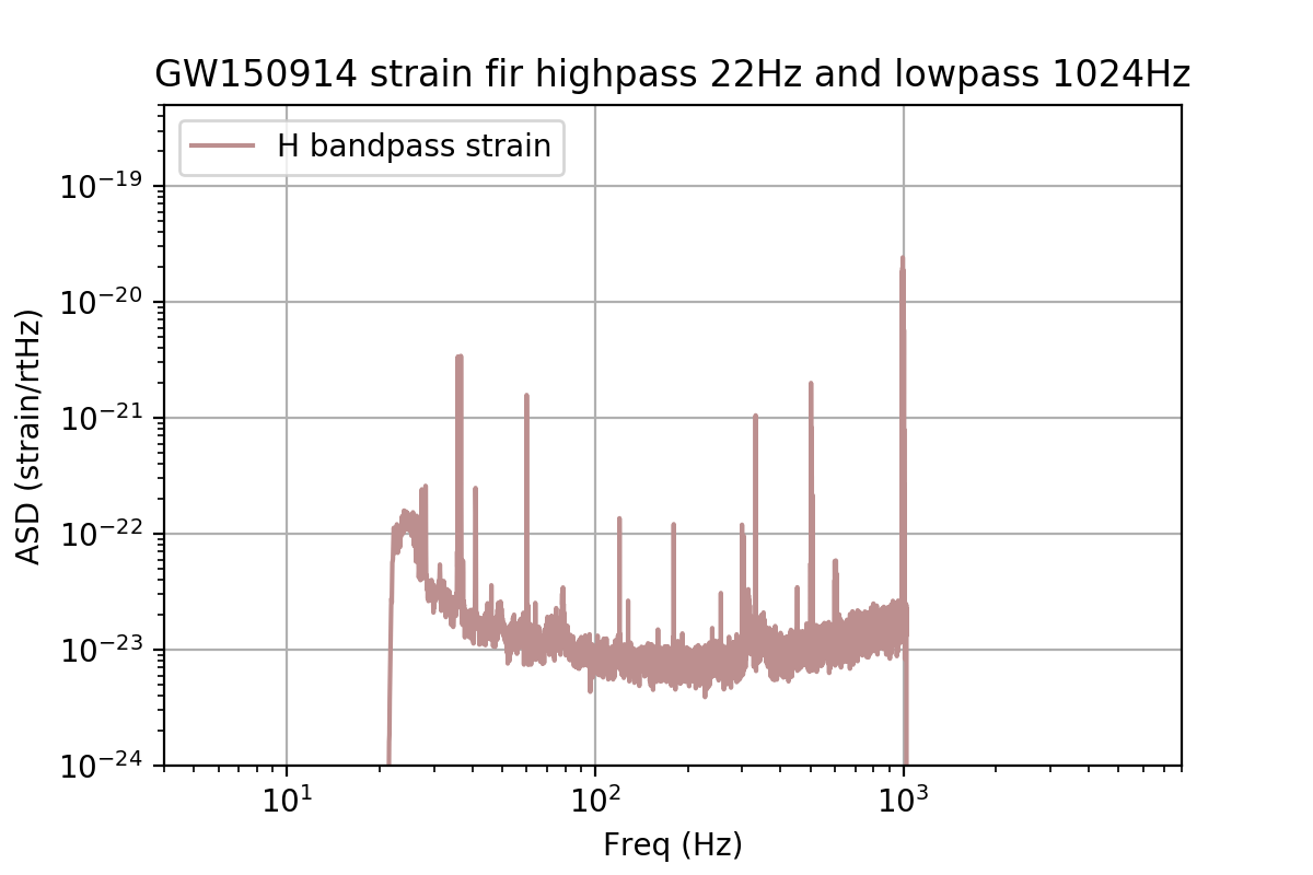
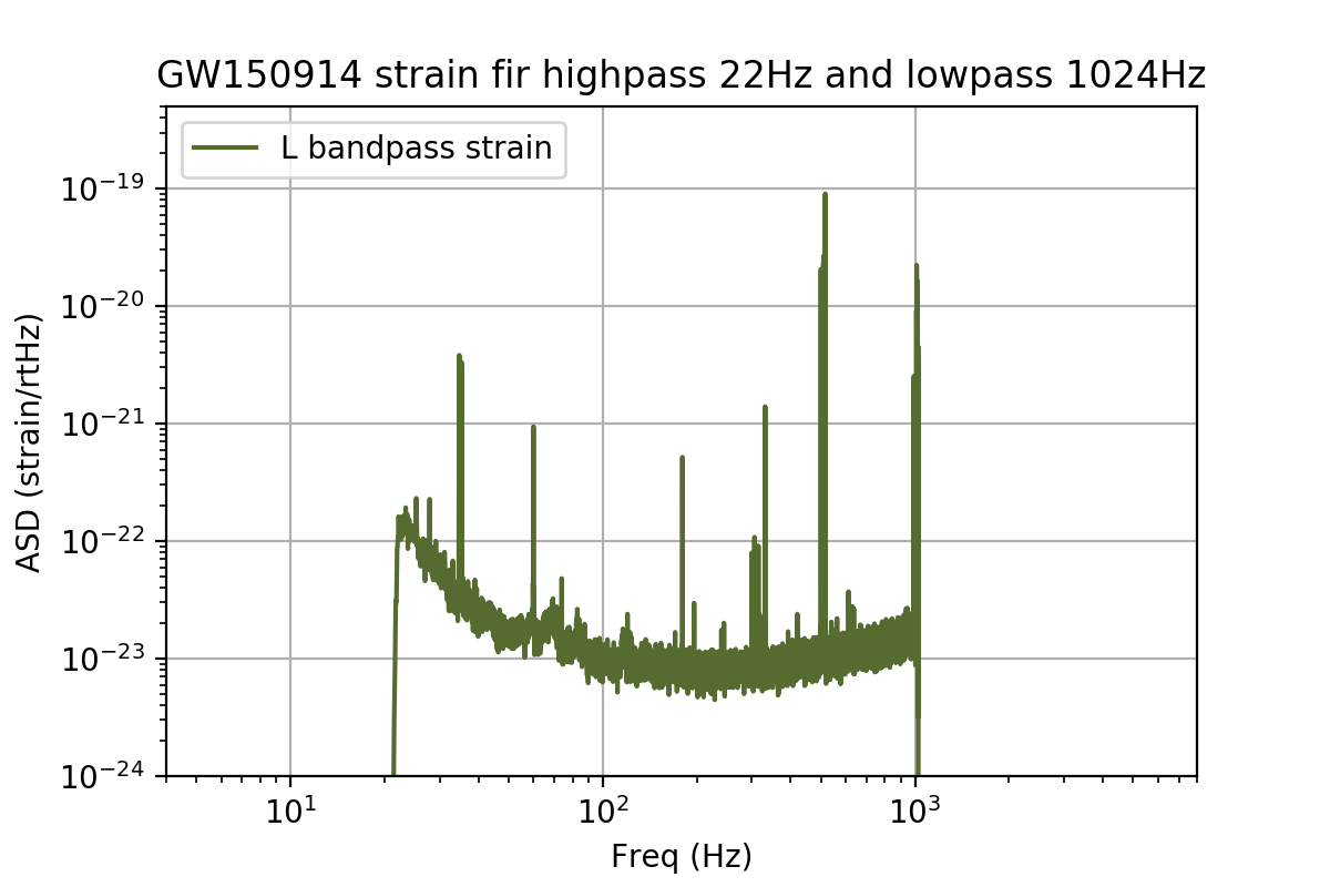
Figure 8: Amplitude spectral density of the strains after bandpass FIR filter at frequencies 22-1024Hz; Hanford on the left and Livingston on the right.

Comparing with the graphs in figure 2 one can see the sharp attenuations at the chosen boundary frequencies. One can still observed the narrow bands of intrinsic detector noise at well defined frequencies; that we handle next.

3.2 Filtering intrinsic detector frequencies

A common way to deal with signals contained in complex noisy data is to apply the whitening filters; that had been using the LIGO Collaboration. Instead of this, we use stopband FIR filters for each of the well defined narrow frequencies generated by each of the detectors.

The first thing to do is to identify precisely the value of the frequency and width of every intrinsic instrumental excitation introduced by each detector in the strain. After this we apply the stopband FIR filter to each strain. Again, to avoid boundary effects, we apply the filter to an interval of length 272s which was obtained from the bandpass strain of 288s by clipping the extremes. Then, we trim again the interval to the desired length of 256s. The result is shown in figure 9.

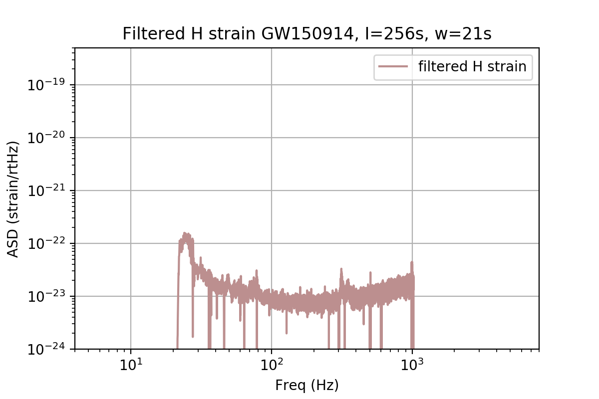
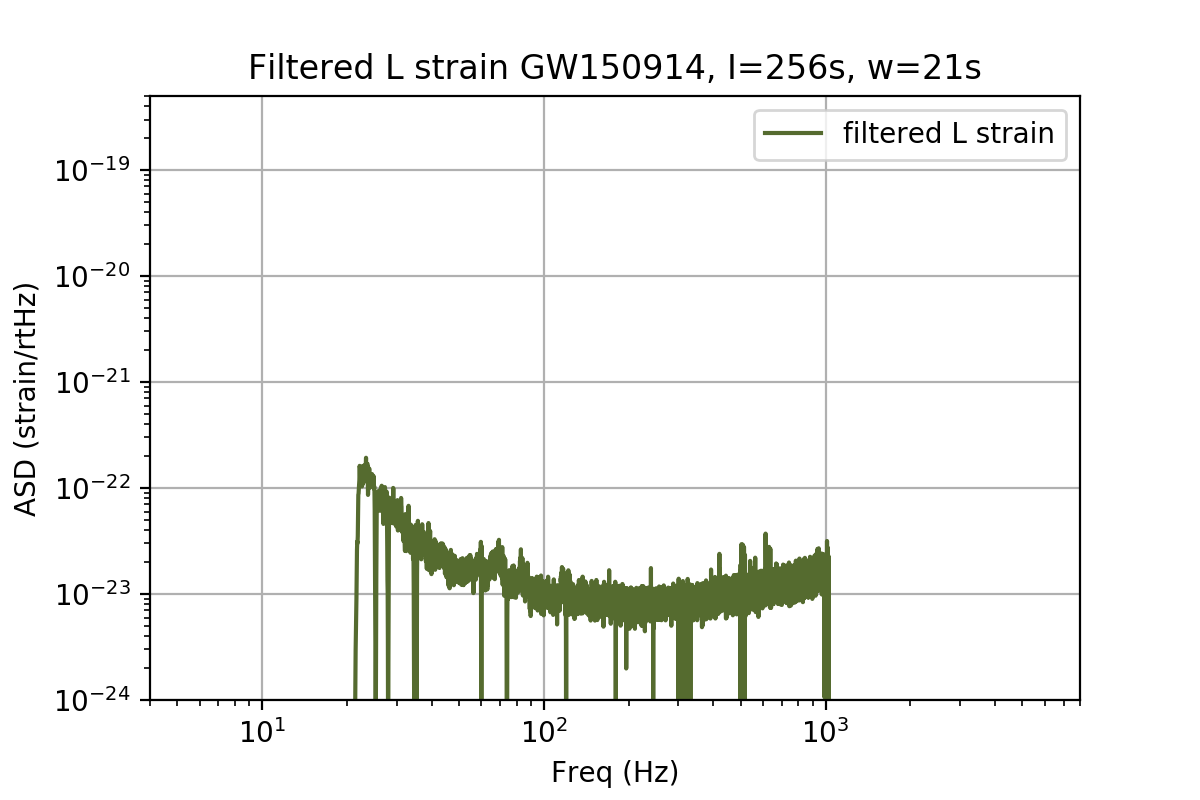
Figure 9: Amplitude spectral density of the strains after bandpass and stopband FIR filter; Hanford on the left and Livingston on the right. We use the same axis limits as in previous graphs in order to facilitate the comparison.

It can be seen that the resulting ASD behavior is fairly flat except for the initial curved behavior at low frequencies; which it could be related to colored noise. The idea behind the decision of not filtering the low frequencies at this stage is that we would like to allow for possible interesting physical signals at this initial portion of the spectrum. Below, we do find such low frequency signals.

The strategy is then to avoid making changes to the astrophysical signal in the pre-processing filtering stage. This is completely different from the approach used up to now in LIGO/Virgo Collaboration articles[1, 2, 16, 17].

3.3 Phase behavior after filtering

In figure 10 we show how the phases are distributed across the frequency range of 22 to 500Hz, on the 256s strain of both detectors, after the first set of FIR filters, bandpass and stopband, have been applied.

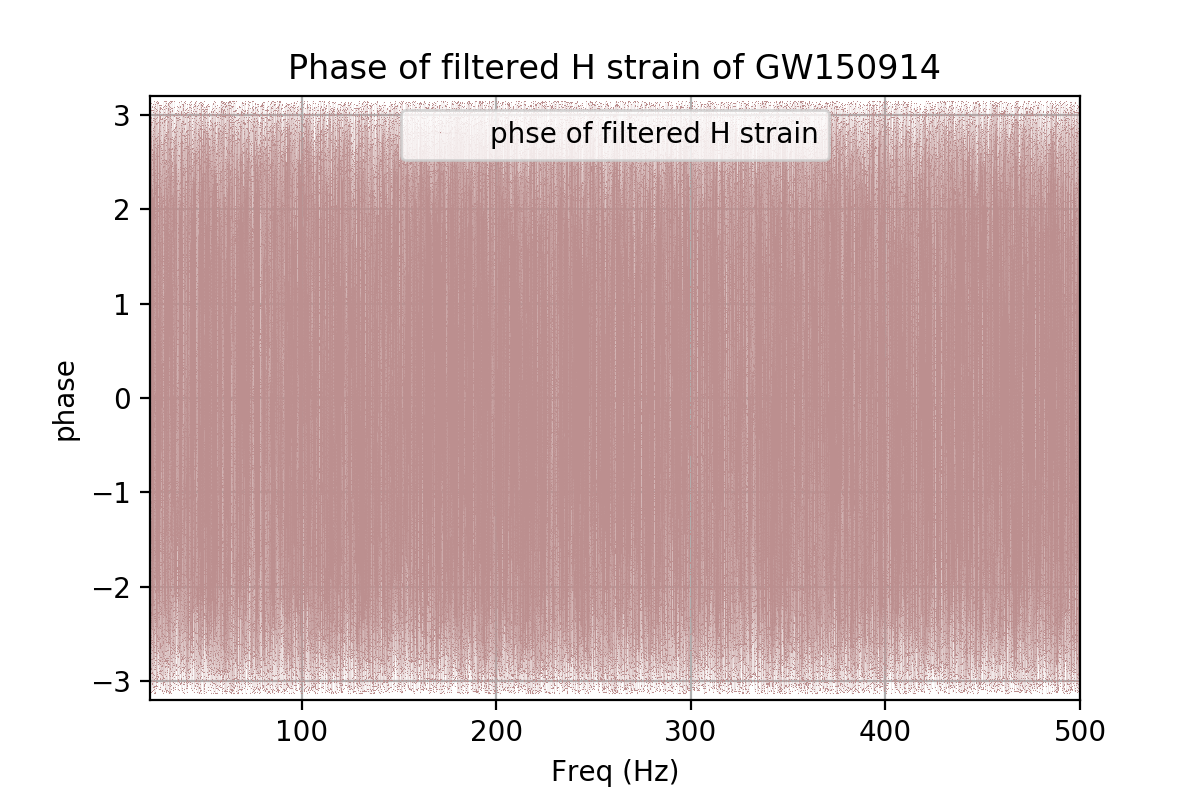
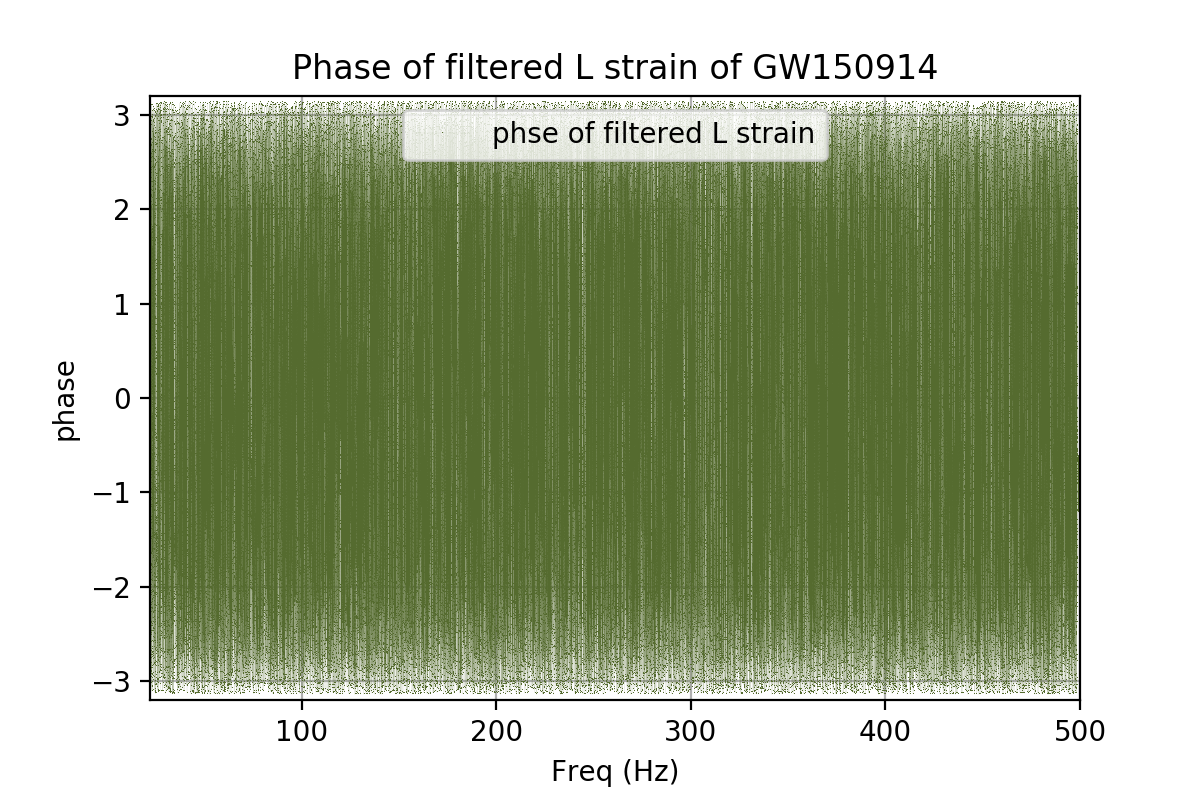
Figure 10: Phase graphs of strains after new first FIR filtering round; Hanford on the left and Livingston on the right.

It can be seen that phases are evenly distributed in the frequency range of interest; which it must be compared with the corresponding phase study after applying the first LIGO filtering procedures to the strains, shown in figure 6.

This is a strong indication that we were able to suppress the initial phase correlation in the raw data; and also that this correlation was due to the intrinsic excitations of the detectors.

Of course an evenly distribution of phases is a good sign, since indicates an almost Gaussian noise behavior.

3.4 Time domain graphs after filtering

Since the initial data is obtained in the time domain, we should see what is the result of our filtering approach in it, and also if we are able to obtain some new insight.

Figure 11 and 12 presents respectively the graph of the H and L strains along with the corresponding LIGO matched templates. To avoid very high frequency contribution from the strain, that is not contained in the template, we have applied for these graphs a lowpass FIR 200Hz filter.

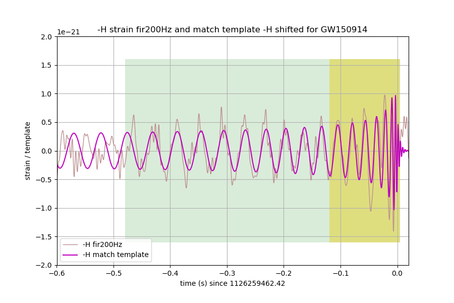
Figure 11: Strain of Hanford detector after a lowpass 200Hz FIR-filter, along with its adjusted by LIGO script template, close to the time of the event.

It can be seen in the figure 11 that there is a remarkable coincidence in frequency, phase and amplitude of the strain and the template in the time interval that goes from about -0.5s to -0.1s before the time of the event; that we have marked with a light green color rectangle. The light yellow band that includes the time of the event, and extends for about 0.1s, is to indicate approximately the lapse of time that is allowed by the whitening LIGO procedure. This was shown in the lower right graph of figure 7 above.

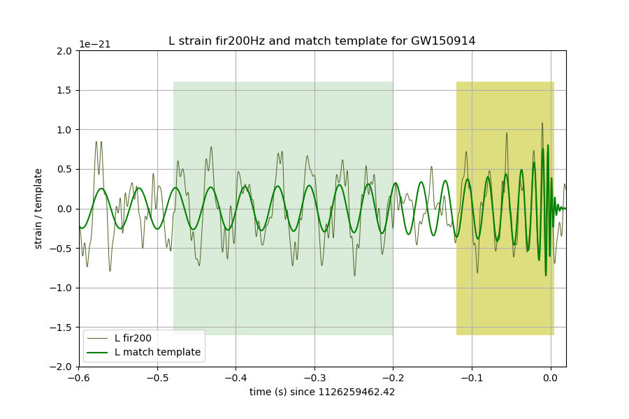
Figure 12: Strain of Livingston detector after a lowpass 200Hz FIR-filter, along with its adjusted by LIGO script template, close to the time of the event.

Observing the Livingston graph of figure 12 one can see that there is a very good agreement in frequency, phase and amplitude of the strain and the template in the time lapse that goes from about -0.5s to -0.2s before the time of the event; that we have marked with a light green color rectangle. There is a short period of time from about -0.2 to -0.1s where the detector could not record properly the signal.

The fact that the same type of indication appears in both detectors invites to present the two sets of data in the same graph, which appears in figure 13.

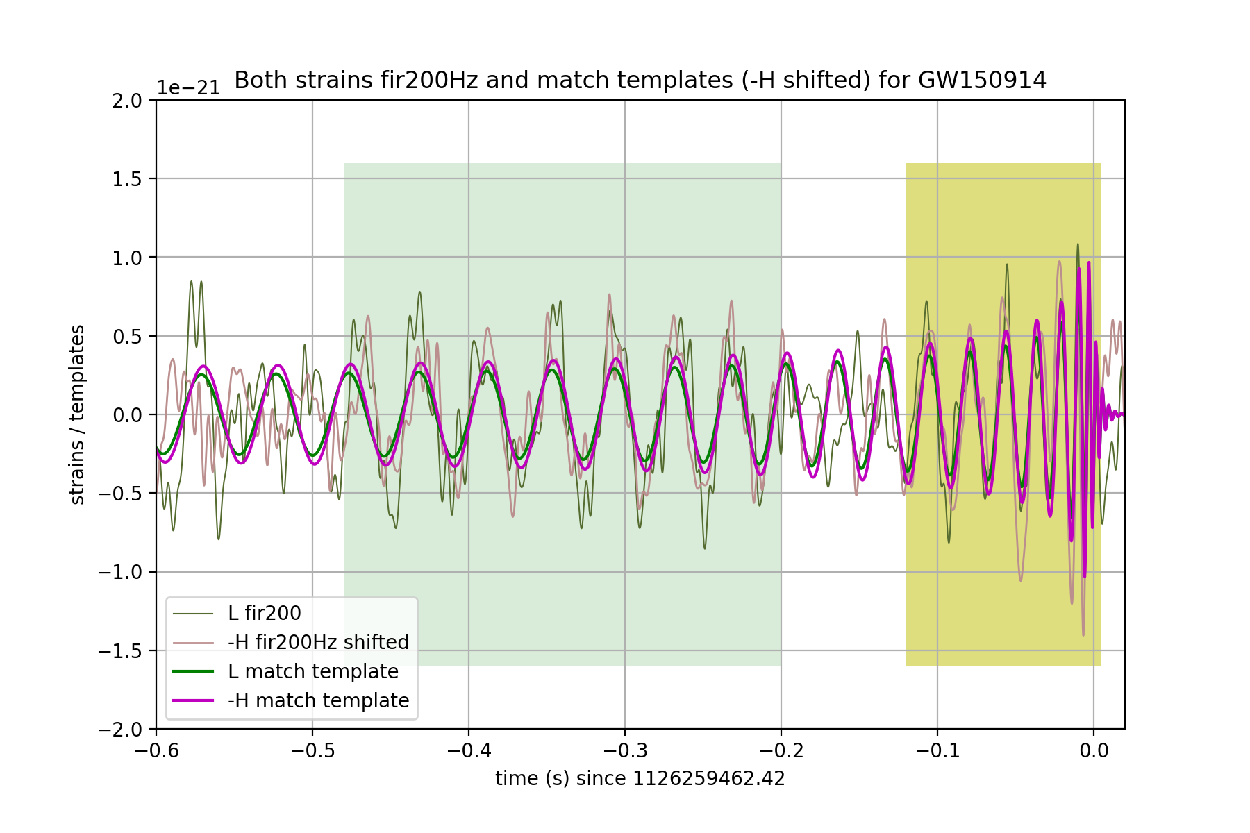
Figure 13: Strain of both detectors after a lowpass 200Hz FIR-filter, along with their adjusted by LIGO script templates, close to the time of the event.

In figure 13 the H strain has been inverted an appropriately shifted, in order to agree in phase at the high amplitude part of the signal with the L strain.

It can be noticed that even if one considers only the light green region in which both detectors show independently a match of the strain with the corresponding templates, we find several coincidences: the shown interval is very close to the event time, at each detector the template matches the strain up to about -0.5s, in phase, amplitude and frequency and very importantly both detectors synchronize in the shown interval. This is compelling evidence that the lapse of time up to about -0.5 seconds before the time of the event contains physically interesting signals. Our findings can be contrasted with the claims in LIGO publications[19] in which they recognize up to 0.2s of signal.

This discovery shows precisely the benefit to use filtering techniques that avoid to change the expected nature of the astrophysical signal.

3.5 Spectrograms of the filtered signals

In figure 14 we present the graphs corresponding to the spectrograms after applying our filters to the data, where one can see that the rising in frequency signals reaches more than 250Hz in the Hanford data, and more than 200Hz in the Livingston one.

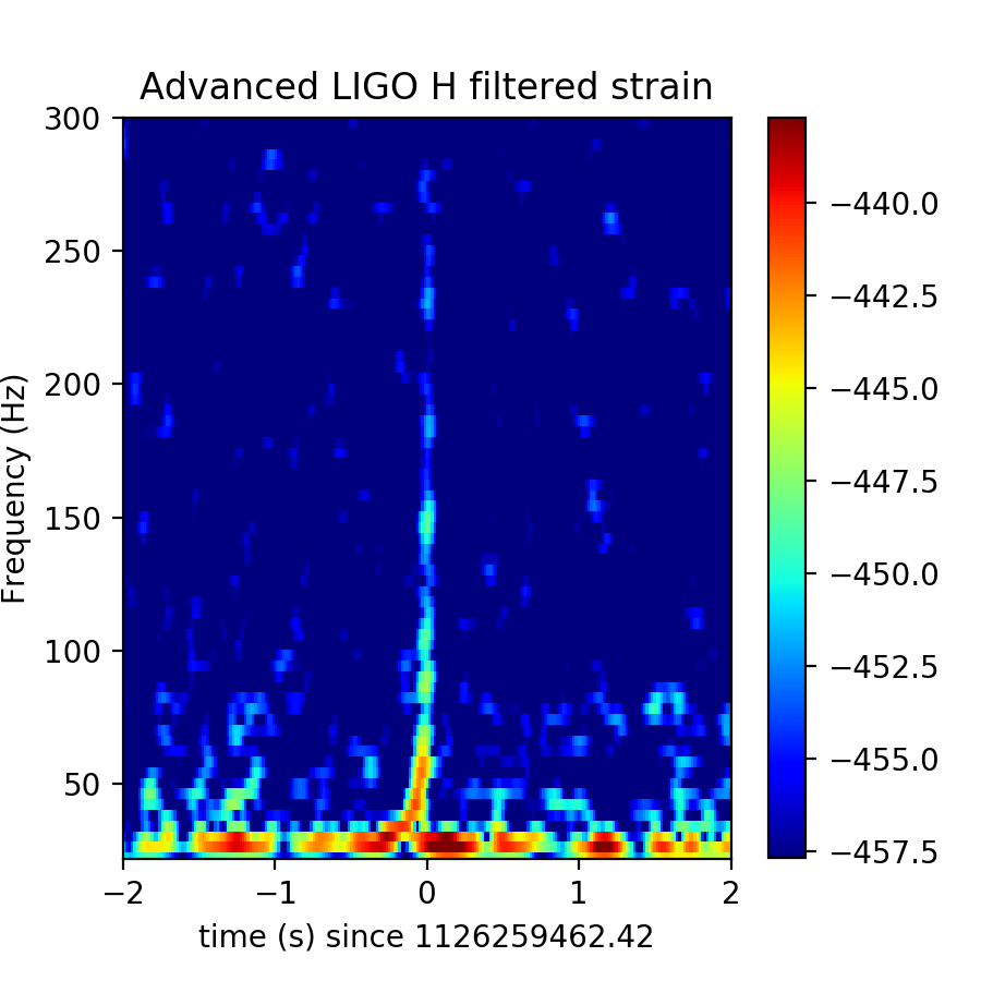
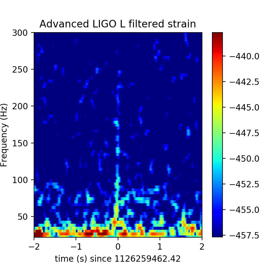
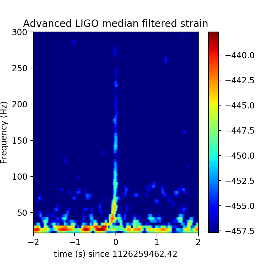
Figure 14: Spectrograms of filtered data from Hanford on the left, and Livingston at the center; $\pm$2 seconds around the time of event GW150914, in the range from 22 to 300Hz. We have also included on the right the corresponding spectrogram for the median; where the H strain has been inverted and shifted.

Due to the chosen directions of the arms of the LIGO detectors, Hanford and Livingston observatories will be sensible to almost the same component of the polarization of the signal. This is the reason why both matched templates are so similar. Because of this one is tempted also to look at the median of both strains, after the corresponding inversion and time shift has been applied to one of the data; since in particular by doing so one expects to obtain better reduction of the noise. For this reason we have also included in the last graph of figure 14 the corresponding spectrogram for the median. There one can see that we have gain some noise reduction and also that there seems to be some coincidence on the data at low frequencies, within the last second before the time of the event; which reinforces our claims observed in the time domain graphs.

4 Final comments

Let us summarize what we have presented so far. In section 2 we have reviewed the basic characteristics of the data of the GW150914 event, and showed the limitations in the pre-processing filtering techniques used in the LIGO Collaboration studies; based on the whitening procedure, and occasionally IIR bandpass filtering.

In order to circumvent the shortcoming of the whitening procedure of too much attenuation for low frequencies, we have presented a new straight forward filtering approach based on FIR filters, in section 3, that performs and initial bandpass, and secondly a careful stopband filter; that yields a minimum touched strain which respects the possibility of low frequency signals.

When observing the effect of our filter on the phase diagrams in figure 10, we deduce that our approach handles successfully the initial correlations of phases shown in the raw data graphs, presented in section 2. In this way we also avoid the awkward phase behavior after applying the LIGO filtering techniques, shown in figure 6.

We have given evidence that, very close to the time of the GW150914 event, in a lapse of time of few tenths of a second: there is coincidence of frequency, amplitude and phase, between the detectors and with their respective templates used by the LIGO Collaboration. It is highly improbable that this concomitance should be attributed just to chance. Therefore, there is more signal to be studied which is encoded in the data of the GW150914 event.

This article is devoted to the presentation of a new approach for the pre-processing of the data; so that we intend to study in detail in separate works the strain we have obtained in this way. For this reason we have not quantified the coincidence of strains at both detectors near the time of the event; we do plan to present this with a new technique to look for similar signals in a pair of detectors, in a separate work. We also intend to apply the filtering approach presented here to all the available gravitational wave data of other events.

We suggest that many of previous analysis of the data, should be carried out after applying the type of filtering we have presented here; instead of the usual whitening pre-processing approach.

Acknowledgments

We are very grateful to the LIGO/Virgo Collaboration for making available the data and the python scripts on data analysis at https://www.gw-openscience.org/.

We thank Emanuel Gallo for a careful reading of the manuscript and for suggestions.

We acknowledge support from CONICET, SeCyT-UNC and Foncyt.

References

- [1] Virgo, LIGO Scientific Collaboration, B. P. Abbott et al., “Observation of Gravitational Waves from a Binary Black Hole Merger,” Phys. Rev. Lett. 116 no. 6, (2016) 061102, arXiv:1602.03837 [gr-qc].
- [2] Virgo, LIGO Scientific Collaboration, B. P. Abbott et al., “Properties of the Binary Black Hole Merger GW150914,” Phys. Rev. Lett. 116 no. 24, (2016) 241102, arXiv:1602.03840 [gr-qc].
- [3] Virgo, LIGO Scientific Collaboration, B. P. Abbott et al., “GW151226: Observation of Gravitational Waves from a 22-Solar-Mass Binary Black Hole Coalescence,” Phys. Rev. Lett. 116 no. 24, (2016) 241103, arXiv:1606.04855 [gr-qc].
- [4] VIRGO, LIGO Scientific Collaboration, B. P. Abbott et al., “GW170104: Observation of a 50-Solar-Mass Binary Black Hole Coalescence at Redshift 0.2,” Phys. Rev. Lett. 118 no. 22, (2017) 221101, arXiv:1706.01812 [gr-qc].
- [5] Virgo, LIGO Scientific Collaboration, B. P. Abbott et al., “GW170814: A Three-Detector Observation of Gravitational Waves from a Binary Black Hole Coalescence,” Phys. Rev. Lett. 119 no. 14, (2017) 141101, arXiv:1709.09660 [gr-qc].
- [6] Virgo, LIGO Scientific Collaboration, B. P. Abbott et al., “GW170817: Observation of Gravitational Waves from a Binary Neutron Star Inspiral,” Phys. Rev. Lett. 119 no. 16, (2017) 161101, arXiv:1710.05832 [gr-qc].
- [7] LIGO Scientific, Virgo, Fermi GBM, INTEGRAL, IceCube, AstroSat Cadmium Zinc Telluride Imager Team, IPN, Insight-Hxmt, ANTARES, Swift, AGILE Team, 1M2H Team, Dark Energy Camera GW-EM, DES, DLT40, GRAWITA, Fermi-LAT, ATCA, ASKAP, Las Cumbres Observatory Group, OzGrav, DWF (Deeper Wider Faster Program), AST3, CAASTRO, VINROUGE, MASTER, J-GEM, GROWTH, JAGWAR, CaltechNRAO, TTU-NRAO, NuSTAR, Pan-STARRS, MAXI Team, TZAC Consortium, KU, Nordic Optical Telescope, ePESSTO, GROND, Texas Tech University, SALT Group, TOROS, BOOTES, MWA, CALET, IKI-GW Follow-up, H.E.S.S., LOFAR, LWA, HAWC, Pierre Auger, ALMA, Euro VLBI Team, Pi of Sky, Chandra Team at McGill University, DFN, ATLAS Telescopes, High Time Resolution Universe Survey, RIMAS, RATIR, SKA South Africa/MeerKAT Collaboration, B. P. Abbott et al., “Multi-messenger Observations of a Binary Neutron Star Merger,” Astrophys. J. 848 no. 2, (2017) L12, arXiv:1710.05833 [astro-ph.HE].
- [8] Virgo, LIGO Scientific Collaboration, B. P. Abbott et al., “GW170608: Observation of a 19-solar-mass Binary Black Hole Coalescence,” arXiv:1711.05578 [astro-ph.HE].
- [9] LIGO Scientific, Virgo Collaboration, B. P. Abbott et al., “GWTC-1: A Gravitational-Wave Transient Catalog of Compact Binary Mergers Observed by LIGO and Virgo during the First and Second Observing Runs,” arXiv:1811.12907 [astro-ph.HE].
- [10] H. Liu and A. D. Jackson, “Possible associated signal with GW150914 in the LIGO data,” JCAP 1610 no. 10, (2016) 014, arXiv:1609.08346 [astro-ph.IM].
- [11] P. Naselsky, A. D. Jackson, and H. Liu, “Understanding the LIGO GW150914 event,” JCAP 1608 no. 08, (2016) 029, arXiv:1604.06211 [astro-ph.CO].
- [12] J. Creswell, S. von Hausegger, A. D. Jackson, H. Liu, and P. Naselsky, “On the time lags of the LIGO signals,” JCAP 1708 no. 08, (2017) 013, arXiv:1706.04191 [astro-ph.IM].
- [13] M. A. Green and J. W. Moffat, “Extraction of black hole coalescence waveforms from noisy data,” Phys. Lett. B784 (2018) 312–323, arXiv:1711.00347 [astro-ph.IM].
- [14] J. Creswell, H. Liu, A. D. Jackson, S. von Hausegger, and P. Naselsky, “Degeneracy of gravitational waveforms in the context of GW150914,” JCAP 1803 no. 03, (2018) 007, arXiv:1803.02350 [gr-qc].
- [15] H. Liu, J. Creswell, S. von Hausegger, A. D. Jackson, and P. Naselsky, “A blind search for a common signal in gravitational wave detectors,” JCAP 1802 no. 02, (2018) 013, arXiv:1802.00340 [astro-ph.IM].
- [16] Virgo, LIGO Scientific Collaboration, B. P. Abbott et al., “GW150914: First results from the search for binary black hole coalescence with Advanced LIGO,” Phys. Rev. D93 no. 12, (2016) 122003, arXiv:1602.03839 [gr-qc].
- [17] Virgo, LIGO Scientific Collaboration, B. P. Abbott et al., “Observing gravitational-wave transient GW150914 with minimal assumptions,” Phys. Rev. D93 no. 12, (2016) 122004, arXiv:1602.03843 [gr-qc].
- [18] S. K. Chatterji, The search for gravitational wave bursts in data from the second LIGO science run. PhD thesis, Massachusetts Institute of Technology, 2005. http://hdl.handle.net/1721.1/34388.
- [19] LIGO Scientific, Virgo Collaboration, B. P. Abbott et al., “Characterization of transient noise in Advanced LIGO relevant to gravitational wave signal GW150914,” Class. Quant. Grav. 33 no. 13, (2016) 134001, arXiv:1602.03844 [gr-qc].