On the expected Betti numbers of the nodal set of random fields

Abstract.

This note concerns the asymptotics of the expected total Betti numbers of the nodal set for an important class of Gaussian ensembles of random fields on Riemannian manifolds. By working with the limit random field defined on the Euclidean space we were able to obtain a locally precise asymptotic result, though due to the possible positive contribution of large percolating components this does not allow to infer a global result. As a by-product of our analysis, we refine the lower bound of Gayet-Welschinger for the important Kostlan ensemble of random polynomials and its generalisation to Kähler manifolds.

1. Introduction

1.1. Betti numbers for random fields: Euclidean case

Let $F:\mathbb{R}^{d}\rightarrow\mathbb{R}$ be a centred stationary Gaussian random field, $d\geq 2$. The nodal set of $F$ is its (random) zero set

$$\mathcal{Z}_{F}:=F^{-1}(0)=\{x\in\mathbb{R}^{d}:\>F(x)=0\}\subseteq\mathbb{R}^{d};$$

assuming $F$ is sufficiently smooth and non-degenerate (or regular), its connected components (“nodal components of $F$”) are a.s. either closed $(d-1)$-manifolds or smooth infinite hypersurfaces (“percolating components”). One way to study the topology of $\mathcal{Z}_{F}$, a central research thread in the recent few years, is by restricting $F$ to a large centred ball $B(R)=\{x\in\mathbb{R}^{d}:\>\|x\|<R\}$, and then investigate the restricted nodal set $\widetilde{\mathcal{Z}_{F}}(R):=F^{-1}(0)\cap B(R)$ as $R\rightarrow\infty$. The set $\widetilde{\mathcal{Z}_{F}}(R)$ consists of the union of the a.s. smooth closed nodal components of $\mathcal{Z}_{F}$ lying entirely in $B(R)$, and the fractions of nodal components of $F$ intersecting $\partial B(R)$; note that, by intersecting with $B(R)$, the components intersecting $\partial B(R)$, finite or percolating, might break into $2$ or more connected components, or fail to be closed.

It follows as a by-product of the precise analysis due to Nazarov-Sodin  [25, 18] that, under very mild assumptions on $F$ to be discussed below, mainly concerning its smoothness and non-degeneracy, with high probability most of the components of $\mathcal{Z}_{F}$ fall into the former, rather than the latter, category (see (1.2) below). That is, for $R$ large, with high probability, most of the components of $\mathcal{Z}_{F}$ intersecting $B(R)$ are lying entirely within $B(R)$. Setting

$$\mathcal{Z}_{F}(R):=\bigcup\limits_{\gamma\subseteq B(R)}\gamma$$

to be the union of all the nodal components $\gamma$ of $F$ lying entirely in $B(R)$, the first primary concern of this note is in the topology of $\mathcal{Z}_{F}(R)$, and, in particular, the Betti numbers of $\mathcal{Z}_{F}(R)$ as $R\rightarrow\infty$, more precisely, the asymptotics of their expected values.

For $0\leq i\leq d-1$ the corresponding Betti number $b_{i}(\cdot)$ is the dimension of the $i$’th homology group, so that a.s.

$$\beta_{i}(R)=\beta_{F;i}(R):=b_{i}(\mathcal{Z}_{F}(R))=\sum\limits_{\gamma\subseteq\mathcal{Z}_{F}(R)}b_{i}(\gamma),$$ (1.1)

summation over all nodal components $\gamma$ lying in $\mathcal{Z}_{F}(R)$. For example, $\beta_{0}=:\mathcal{N}_{F}(R)$ is the total number of connected components $\gamma\subseteq\mathcal{Z}_{F}(R)$ (“nodal count”) analysed by Nazarov-Sodin, and

$$\beta_{i}(R)=\beta_{d-1-i}(R)$$

by Poincaré duality. To be able to state Nazarov-Sodin’s results we need to introduce the following axioms; by convention they are expressed in terms of the spectral measure rather than $F$ or its covariance function.

Definition 1.1 (Axioms $(\rho 1)-(\rho 4)$ on $F$).

Let $F:\mathbb{R}^{d}\rightarrow\mathbb{R}$ be a Gaussian stationary random field,

$$r_{F}(x-y)=r_{F}(x,y):=\mathbb{E}[F(x)\cdot F(y)]$$

the covariance function of $F$, and $\rho=\rho_{F}$ be its spectral measure, i.e. the Fourier transform of $r_{F}$ on $\mathbb{R}^{d}$.

1. $F$ satisfies $(\rho 1)$ if the measure $\rho$ has no atoms.

2. $F$ satisfies $(\rho 2)$ if for some $p>6$,

   $$\int\limits_{\mathbb{R}^{d}}\|\lambda\|^{p}d\rho(\lambda)<\infty.$$

3. $F$ satisfies $(\rho 3)$ if the support of $\rho$ does not lie in a linear hyperplane of $\mathbb{R}^{d}$.

4. $F$ satisfies $(\rho 4)$ if the interior of the support of $\rho$ is non-empty.

Axioms $(\rho 1)$, $(\rho 2)$ and $(\rho 3)$ ensure that the action of translations on $\mathbb{R}^{d}$ is ergodic, a.s. sufficient smoothness of $F$, and non-degeneracy of $F$ understood in proper sense, respectively. Axiom $(\rho 4)$ implies that any smooth function belongs to the support of the law of $F$, which, in turn, will yield the positivity of the number of nodal components, and positive representation of every topological type of nodal components.

Recall that $\mathcal{N}_{F}(R)=\beta_{0}(R)$ is the number of nodal components of $F$ entirely lying in $B(R)$, and let $V_{d}$ be the volume of the unit $d$-ball, and $\operatorname{Vol}B(R)=V_{d}\cdot R^{d}$ be the volume of the radius $R$ ball in $\mathbb{R}^{d}$. Nazarov and Sodin  [25, 18] proved that if $F$ satisfies $(\rho 1)-(\rho 3)$, then there exists a constant $c_{NS}=c_{NS}(\rho_{F})$ (“Nazarov-Sodin constant”) so that $\frac{\mathcal{N}_{F}(R)}{\operatorname{Vol}B(R)}$ converges to $c_{NS}$, both in mean and a.s. That is, as $R\rightarrow\infty$,

$$\mathbb{E}\left[\left|\frac{\mathcal{N}_{F}(R)}{\operatorname{Vol}B(R)}-c_{NS}\right|\right]\rightarrow 0,$$ (1.2)

so that, in particular,

$$\mathbb{E}[\mathcal{N}_{F}(R)]=c_{NS}\cdot\operatorname{Vol}B(R)+o(R^{d}).$$ (1.3)

They also showed that imposing $(\rho 4)$ is sufficient (but not necessary) for the strict positivity of $c_{NS}$, and found other very mild sufficient conditions on $\rho$, so that $c_{NS}>0$. The validity of the asymptotic (1.3) for the expected nodal count was extended  [14] to hold without imposing the ergodicity axiom $(\rho 1)$, with $c_{NS}=c_{NS}(\rho_{F})$ appropriately generalised, also establishing a stronger estimate for the error term as compared to the r.h.s. of (1.3).

One might think that endowing the “larger” components with the same weight $1$ as the “smaller” components might be “discriminatory” towards the larger ones, so that separating the counts based on the components’ topology  [24] or geometry  [3] would provide an adequate response for the alleged discrimination. These nevertheless do not address the important question of the total Betti number $\beta_{i}$, the main difficulty being that the individual Betti number $b_{i}(\gamma)$ of a nodal component $\gamma$ of $F$ is not bounded, even under the assumption that $\gamma\subseteq B(R)$ is entirely lying inside a compact domain. Despite this, we will be able to resolve this difficulty by controlling from above the total Betti number via Morse Theory  [16], an approach already pursued by Gayet-Welschinger  [10] (see §2 below for a more detailed explanation).

Theorem 1.2.

Let $F:\mathbb{R}^{d}\rightarrow\mathbb{R}$ be a centred Gaussian random field, satisfying axioms $(\rho 2)$ and $(\rho 3)$ of Definition 1.1, $d\geq 2$, and $0\leq i\leq d-1$. Then

1. There exists a number $c_{i}=c_{F;i}\geq 0$ so that

   $$\mathbb{E}[\beta_{i}(R)]=c_{i}\cdot\operatorname{Vol}B(R)+o_{R\rightarrow\infty}(R^{d}).$$ (1.4)

2. If, in addition, $F$ satisfies $(\rho 1)$, then convergence (1.4) could be extended to hold in mean, i.e.

   $$\mathbb{E}\left[\left|\frac{\beta_{i}(R)}{\operatorname{Vol}B(R)}-c_{i}\right|\right]\rightarrow 0$$ (1.5)

   as $R\rightarrow\infty$.

3. Further, if $F$ satisfies the axiom $(\rho 4)$ (in addition to $(\rho 2)$ and $(\rho 3)$, but not $(\rho 1)$), then $c_{i}>0$. The same conclusion holds for the important Berry’s monochromatic isotropic random waves in arbitrary dimensions (“Berry’s random wave model”).

1.2. Motivation and background

The Betti numbers of both the nodal and the excursion sets of Gaussian random fields serve as their important topological descriptor, and are therefore addressed in both mathematics and experimental physics literature, in particular cosmology  [21]. From the complex geometry perspective Gayet and Welschinger  [10] studied the distribution of the total Betti numbers of the zero set for the Kostlan Gaussian ensemble of degree $n$ random homogeneous polynomials on the $d$-dimensional projective space, and their generalisation to Kähler manifolds, $n\rightarrow\infty$. In the projective coordinates $x=[x_{0}:\ldots:x_{d}]\in\mathbb{R}\mathcal{P}^{d}$ we may write

$$P_{n}(x)=\sum\limits_{|j|=n}\sqrt{{n\choose j}}a_{j}x^{j},$$ (1.6)

where $j=(j_{0},\ldots,j_{d})$, $|j|=\sum\limits_{i=0}^{d}j_{i}$, $x^{j}=x_{0}^{j_{0}}\cdot\ldots\cdot x_{d}^{j_{d}}$, ${n\choose j}=\frac{n!}{j_{0}!\cdot\ldots\cdot j_{d}!}$, and $\{a_{j}\}$ are standard Gaussian i.i.d. By the homogeneity of $P_{n}$, its zero set makes sense on the projective space. The Kostlan (also referred to as “Shub-Smale”) ensemble is an important model of random polynomials, uniquely invariant w.r.t. unitary transformations on $\mathbb{C}\mathcal{P}^{d}$. Restricted to the unit sphere $\mathcal{S}^{d}\subseteq\mathbb{R}^{d+1}$, the random fields $P_{n}$ are defined by the covariance function

$$\mathbb{E}[P_{n}(x)\cdot P_{n}(y)]=\langle x,y\rangle^{n}=\left(\cos(\theta(x,y))\right)^{n},$$

where $x,y\in\mathcal{S}^{d}$, the inner product $\langle\cdot,\cdot\rangle$ is inherited from $\mathbb{R}^{d+1}$, and $\theta(\cdot,\cdot)$ is the angle between two points on $\mathbb{R}^{d+1}$.

Upon scaling by $\sqrt{n}$ (the meaning is explained in Definition 1.3 below), the Kostlan polynomials (1.6) admit  [25, §2.5.4], locally uniformly, a (stationary isotropic) limit random field on $\mathbb{R}^{d}$, namely the Bargmann-Fock ensemble defined by the “Gaussian” covariance kernel

$$\kappa(x):=e^{-x^{2}/2},$$ (1.7)

see also  [2, 4]. This indicates that one should expect the Betti numbers to be of order of magnitude $\approx n^{d/2}$. That this is so is supported by Gayet-Welschinger’s upper bounds  [10]

$$\mathbb{E}[b_{i}(P_{n}^{-1}(0))]\leq A_{i}n^{d/2}$$

with some semi-explicit $A_{i}>0$, and the subsequent lower bounds  [9]

$$\mathbb{E}[b_{i}(P_{n}^{-1}(0))]\geq a_{i}n^{d/2},$$ (1.8)

$a_{i}>0$, but to our best knowledge the important question of the true asymptotic behaviour of $b_{i}(P_{n}^{-1}(0))$ is still open.

1.3. Betti numbers for Gaussian ensembles on Riemannian manifolds

Since $\kappa$ of (1.7) (or, rather, its Fourier transform) easily satisfies all Nazarov-Sodin’s axioms $(\rho 1)-(\rho 4)$ of Definition 1.1, one wishes to invoke Theorem 1.2 with the Bargmann-Fock field in place of $F$, and try to deduce the results analogous to (1.4) for the Betti numbers of the nodal set of $P_{n}$ in (1.6). This is precisely the purpose of Theorem 1.5 below, valid in a scenario of local translation invariant limits, far more general than merely the Kostlan ensemble, whose introduction is our next goal.

Let $\mathcal{M}$ be a compact Riemannian $d$-manifold, and $\{f_{L}\}_{L\in\mathcal{L}}$ be a family of smooth Gaussian random fields $f_{L}:\mathcal{M}\rightarrow\mathbb{R}$, where the index $L$ attains a discrete set $\mathcal{L}$, and $K_{L}(\cdot,\cdot)$ the covariance function corresponding to $f_{L}$, so that

$$K_{L}(x,y)=\mathbb{E}[f_{L}(x)\cdot f_{L}(y)];$$

the parameter $L$ should be thought of as the scaling factor, generalising the rolse of $\sqrt{n}$ for the Kostlan ensemble. We scale $f_{L}$ restricted to a sufficiently small neighbourhood of a point $x\in\mathcal{M}$, so that the exponential map $\exp_{x}(\cdot):T_{x}\mathcal{M}\rightarrow\mathcal{M}$ is well defined. We define

$$f_{x,L}(u):=f_{L}(\exp_{x}(u/L),$$ (1.9)

with covariance

$$K_{x,L}(u,v):=K_{L}(\exp_{x}(u/L),\exp_{x}(v/L))$$

with $|u|,|v|<L\cdot r$ with $r$ sufficiently small, uniformly with $x\in\mathcal{M}$, allowing $u,v$ to grow with $L\rightarrow\infty$.

Definition 1.3 (Local translation invariant limits, cf.  [18, Definition 2 on p. 6]).

We say that the Gaussian ensemble $\{f_{L}\}_{L\in\mathcal{L}}$ possesses local translation invariant limits, if for almost all $x\in\mathcal{M}$ there exists a positive definite function $K_{x}:\mathbb{R}^{d}\rightarrow\mathbb{R}$, so that for all $R>0$,

$$\lim\limits_{L\rightarrow\infty}\sup\limits_{|u|,|v|\leq R}\left|K_{x,L}(u,v)-K_{x}(u-v)\right|\rightarrow 0.$$ (1.10)

Important examples of Gaussian ensembles possessing translation invariant local limits include (but not limited to) Kostlan’s ensemble (1.6) of random homogeneous polynomials, and Gaussian band-limited functions  [24], i.e. Gaussian superpositions of Laplace eigenfunctions corresponding to eigenvalues lying in an energy window. For manifolds with spectral degeneracy, such as the sphere and the torus (and $d$-cube with boundary), the monochromatic random waves (i.e. Gaussian superpositions of Laplace eigenfunctions belonging to the same eigenspace) are a particular case of band-limited functions; two of the most interesting cases are those of random spherical harmonics (random Laplace eigenfunctions on the round unit $d$-sphere)  [26, 27], and “Arithmetic Random Waves” (random Laplace eigenfunctions on the standard $d$-torus)  [20, 13].

In all the said examples of Gaussian ensembles on manifolds of our particular interest the scaling limit $K_{x}$ (and the associate Gaussian random field on $\mathbb{R}^{d}$) was independent of $x$, and the limit in (1.10) is uniform, attained in a strong quantitative form, see the discussion in  [5, §2.1]. We will also need the following, more technical concepts of uniform smoothness and non-degeneracy for $\{f_{L}\}$, introduced in  [25, definitions 2-3, p. 14-15].

Definition 1.4 (Smoothness and non-degeneracy).

1. We say that $\{f_{L}\}$ is $C^{3-}$ smooth if for every $0<R<\infty$,

   $$\limsup\limits_{L\rightarrow\infty}\sup\left\{|\partial_{u}^{i}\partial^{j}_{v}K_{x,L}(u,v)|:\>|i|,|j|\leq 3;\;x\in\mathcal{M},\|u\|,\|v\|\leq R\right\}<\infty.$$

2. We say that $\{f_{L}\}$ is non-degenerate if for every $0<R<\infty$

   $$\liminf\limits_{L\rightarrow\infty}\inf\left\{\mathbb{E}\left[\partial_{\xi}f_{x,L}(u)^{2}\right]:\>\xi\in\mathcal{S}^{d-1},\,x\in\mathcal{M},\,\|u\|\leq R\right\}>0.$$

Let $\{f_{L}\}_{L\in\mathcal{L}}$ be a $C^{3-}$ smooth, non-degenerate, Gaussian ensemble possessing translation invariant local limits $K_{x}$, corresponding to Gaussian random fields on $R^{d}$ with spectral measure $\rho_{x}$, satisfying axioms $(\rho 1)-(\rho 3)$. Denote $\mathcal{N}(f_{L};x,R/L)$ to be the number of nodal components of $f_{L}$ lying entirely in the geodesic ball $B_{x}(R/L)\subseteq\mathcal{M}$, and $\mathcal{N}(f_{L})$ to be the total number of the nodal components of $f_{L}$ on $\mathcal{M}$. In this settings Nazarov-Sodin  [25, 18] proved that

$$\lim\limits_{R\rightarrow\infty}\limsup\limits_{L\rightarrow\infty}\mathbb{E}\left[\left|\frac{\mathcal{N}(f_{L};x,R/L)}{\operatorname{Vol}B(R)}-c_{NS}(\rho_{x})\right|\right]=0,$$ (1.11)

with $c_{NS}(\cdot)$ same as in (1.2).

For the total number $\mathcal{N}(f_{L})$ they glued the local results (1.11), to deduce, on invoking a two-parameter analogue of Egorov’s Theorem yielding the almost uniform convergence of (1.11) w.r.t. $x$, that

$$\lim\limits_{R\rightarrow\infty}\mathbb{E}\left[\left|\frac{\mathcal{N}(f_{L})}{V_{d}L^{d}}-\nu\right|\right]\rightarrow 0,$$ (1.12)

holds with

$$\nu:=\int\limits_{\mathcal{M}}c_{NS}(\rho_{x})dx.$$

In particular, (1.12) yields

$$\mathbb{E}[\mathcal{N}(f_{L})]=V_{d}\nu\cdot L^{d}+o(L^{d}),$$ (1.13)

As it was mentioned above, in practice, in many applications, the scaling limit $K_{x}(\cdot)\equiv K(\cdot)$ does not depend on $x$, so that, assuming w.l.o.g. that $\operatorname{Vol}(\mathcal{M})=1$, the asymptotic constant $\nu$ in (1.12) (and (1.13)) is $\nu=c_{NS}(\rho)$, where $\rho$ is the Fourier transform of $K$. In this situation, in accordance with Theorem 1.2c, $\nu=c_{NS}>0$ is positive, if $(\rho 4)$ is satisfied. The following result extends (1.11) to arbitrary Betti numbers.

Theorem 1.5.

Let $\{f_{L}\}_{L\in\mathcal{L}}$ be a $C^{3-}$ smooth, non-degenerate, Gaussian ensemble, $x\in\mathcal{M}$ satisfying (1.10) with some $K_{x}$ satisfying axioms $(\rho 1)-(\rho 3)$, and $0\leq i\leq d-1$. Denote $\beta_{i;L}(x,R/L)=\beta_{i}(f_{L};x,R/L)$ to be the total $i$’th Betti number of the union of all components of $f_{L}^{-1}(0)$ entirely contained in the geodesic ball $B_{x}(R/L)$. Then for every $\epsilon>0$

$$\lim\limits_{R\rightarrow\infty}\limsup\limits_{L\rightarrow\infty}\mathcal{P}r\left\{\left|\frac{\beta_{i;L}(x,R/L)}{\operatorname{Vol}B(R)}-c_{i}\right|>\epsilon\right\}=0.$$ (1.14)

where $c_{i}$ is the same as in (1.5), corresponding to the random field defined by $K_{x}$.

Theorem 1.5 asserts that the random variables $\left\{\frac{\beta_{i;L}(x,R/L)}{\operatorname{Vol}B(R)}\right\}_{L\in\mathcal{L}}$ converge in probability to $c_{i}$, in the double limit $L\rightarrow\infty$, and then $R\rightarrow\infty$. One would be tempted to try to deduce the convergence in mean for the same setting, the main obstacle being that $\beta_{i;L}(x,R/L)$ is not bounded, and, in principle, a small probability event might contribute positively to the expectation of $\beta_{i;L}(x,R/L)$. While it is plausible (if not likely) that a handy bound on the variance (or the second moment), such as  [7, 17], for the critical points number would rule this out and establish the desired $L^{1}$-convergence in this, or, perhaps, slightly more restrictive scenario, we will not pursue this direction in the present manuscript, for the sake of keeping it compact.

Theorem 1.5 applied on the Kostlan ensemble (1.6) of random polynomials, in particular, recovers Gayet-Welschinger’s later lower bound (1.8), but, finer, with high probability, it prescribes the asymptotics of the total Betti numbers of all the components lying in geodesic balls of radius slightly above $1/\sqrt{n}$, and hence, in this case, one might think of Theorem 1.5 as a refinement of (1.8). It would be desirable to determine the true asymptotic law of $\mathbb{E}[b_{i}(P_{n}^{-1}(0))]$ (hopefully, for the more general scenario), though the possibility of giant (“percolating”) components is a genuine consideration, and, if our present understanding of this subtlety is correct  [5], then, to resolve the asymptotics of $\mathbb{E}[b_{i}(P_{n}^{-1}(0))]$ the question whether they consume a positive proportion of the total Betti numbers cannot be possibly avoided. In fact, it is likely that for $d\geq 3$, with high probability, there exists a single percolating component consuming a high proportion of the space, and contributing positively to the Betti numbers, as found numerically by Barnett-Jin (presented within  [24]), and explained by P. Sarnak  [22], with the use of percolating vs. non-percolating random fields (see  [5, §1.2] for more details, and also the discussion in §2 below).

1.4. Acknowledgement

It is a pleasure to thank P. Sarnak and M. Sodin for their comments on the presented proofs of the main results, D. Panov for freely sharing his expertise on various aspects of the presented material, Z. Rudnick for his support and encouragement regarding this work and his valuable comments on an earlier version of this manuscript, and Z. Kabluchko for pointing out the superadditive ergodic theorem  [12, Theorem 2.14, page 210]. The author of this manuscript is grateful to D. Beliaev and S. Muirhead for many stimulating conversations concerning subjects of high relelvance to the presented research. The research leading to these results has received funding from the European Research Council under the European Union’s Seventh Framework Programme (FP7/2007-2013), ERC grant agreement n${}^{\text{o}}$ 335141.

2. Outline of the proofs and discussion

2.1. Outline of the proofs of the principle results

The principal novel result of this manuscript is Theorem 1.2. Theorem 1.2 given, the proof of Theorem 1.5 does not differ significantly from the proof of  [25, Theorem 5] given  [25, Theorem 1]. The key observation here is that while passing from the Euclidean random field $F_{x}$ to its perturbed Riemannian version $f_{x,L}$ in the vicinity of $x\in\mathcal{M}$, the topology of its nodal set is preserved on a high probability stable event, to be constructed, and hence so is its $i$’th Betti number. In fact, this was the conclusion from the argument presented in  [24, Theorem 6.2] that will reconstructed in §4, alas briefly, for the sake of completeness.

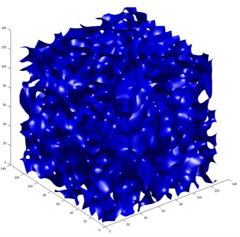
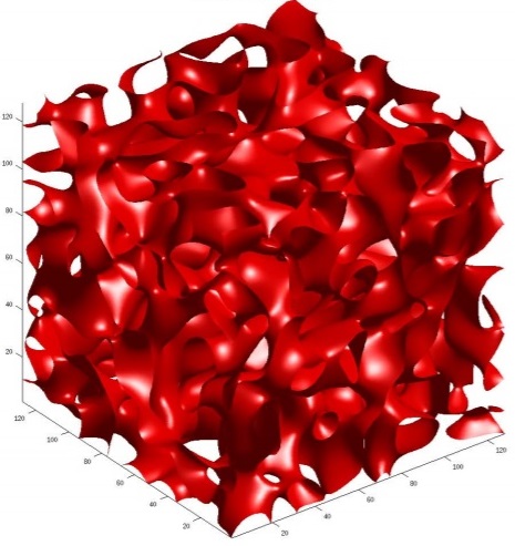
Figure 1. Computer simulations by A. Barnett. Left: Giant percolating nodal components for $3$-dimensional monochromatic isotropic waves. Right: Analogous picture for the “Real Fubini-Study” (a random ensemble of homogeneous polynomials, with different law as compared to Kostlan’s ensemble).

To address the asymptotic expected nodal count $\mathcal{N}_{F}(R)=\beta_{F;0}(R)$, Nazarov-Sodin have developed the so-called Integral Geometric sandwich. The idea is that one bounds, $\mathcal{N}_{F}(R)$ from below using $\mathcal{N}_{\cdot}(r)$, of radii $0<r<R$ much smaller than $R$ (“fixed”), and $F$ translated (equivalently, shifter radius-$r$ ball), and from above using a version of $\mathcal{N}_{F}(r)$, where, rather than counting nodal components lying entirely in $B(r)$ (or its shift), we also include those components intersecting its boundary $\partial B(r)$. By invoking ergodic methods one shows that both these bounds converge to the same limit, and in its turn this yields automatically both the asymptotics for the expected nodal count, and the convergence in mean.

Unfortunately, since we endow each nodal component $\gamma$ with the, possibly unbounded, weight $b_{i}(\gamma)$, the upper bound in the sandwich does not seemingly yield a useful result. We bypass this major obstacle by using a global bound on the expected Betti numbers via Morse Theory (and the Kac-Rice method), and then establishing an asymptotics for the expected number. Rather than working with arbitrary chosen “fixed” radii $r>0$, we only work with “good” radii, defined so that these numbers are “almost maximising” the expected Betti numbers, so that we can infer the same for all the sufficiently big radii $R>r$ (see (3.11) and (3.13)). In hindsight, we interpret working with the good radii as “miraculously” eliminating the possible fluctuations in the contribution to the Betti numbers of the giant percolating domains. Once the asymptotics for the expected Betti number has been determined, we tour de force working with the good radii to also yield the convergence in mean, with the help of the ergodic assumption $(\rho 1)$.

Another possible strategy for proving results like Theorem 1.2 is by observing that, by naturally extending the definition of $\beta_{i}$ to smooth domains $\mathcal{D}\subseteq\mathbb{R}^{d}$ as

$$\beta_{i}(\mathcal{D})=\beta_{i;F}(\mathcal{D}):=\sum\limits_{\gamma\subseteq\mathcal{D}}b_{i}(\gamma),$$

with summation over the (random) nodal components of $F$ lying in $\mathcal{D}$, $\beta_{i}(\cdot)$ is made into a super-additive random variable, i.e. for all $\mathcal{D}_{1},\ldots,\mathcal{D}_{k}\subseteq\mathbb{R}^{d}$ pairwise disjoint domains, the inequality

$$\beta_{i}\left(\bigcup\limits_{j=1}^{k}\mathcal{D}_{j}\right)\geq\sum\limits_{j=1}^{k}\beta_{i}(\mathcal{D}_{j})$$

holds. It then might be tempting to apply the superadditive ergodic theorem  [12, Theorem 2.14, page 210] (and its finer version  [19, p. 165]) on $\beta_{i}$. However, in this manuscript we will present a direct and explicit treatise of this subject.

2.2. Discussion

As it was mentioned above, a straightforward application of 1.5 on the Kostlan’s ensemble of random homogenous polynomials, in particular implies the lower bound (1.8) for the total expected Betti number for this ensemble due to Gayet-Welschinger, and its generalisations for Kähler manifolds. Our argument is entirely different as compared to Gayet-Welschinger’s: rather than working with the finite degree polynomials  (1.6), as in  [9], we first prove the result for the limit Bargmann-Fock random field on $\mathbb{R}^{d}$ (Theorem 1.2), and then deduce the result by a perturbative procedure following Nazarov-Sodin (Theorem 1.5).

It is crucial to determine whether the global asymptotics

$$\mathbb{E}[\beta_{i;L}]\sim c_{i}\operatorname{Vol}(\mathcal{M})\cdot L^{d},$$

expected from its local probabilistic version (1.14), could be extended to hold for the total expected Betti number of $f^{-1}$ in some scenario, inclusive of all the motivational examples. Such a result would indicate that no giant “percolating” components, not lying inside any macroscopic (or slightly bigger) geodesic balls exist, contributing positively to the Betti numbers. In fact some numerics due to Barnett-Jin (presented within  [24]) support the contrary for $d\geq 3$, as argued by Sarnak  [22], see Figure 1, and also  [5, §2.1]. To our best knowledge, at this stage this question is entirely open, save for the results on $\beta_{0;L}$ (and $\beta_{d-1;L}$) due to Nazarov-Sodin.

3. Proof of Theorem 1.2

3.1. Auxiliary lemmas

Recall that $\beta_{i}(R)=b_{i}(\mathcal{Z}_{F}(R))$ is defined in (1.1), and for $x\in\mathbb{R}^{d}$, $R>0$, introduce

$$\beta_{i}(x;R)=\beta_{F;i}(x,R):=\sum\limits_{\gamma\subseteq\mathbb{Z}_{F}\cap B_{x}(R)}b_{i}(\gamma),$$ (3.1)

summation over all nodal components of $F$ contained in the shifted ball $B_{x}(R)$, or, equivalently

$$\beta_{F;i}(x,R)=\beta_{T_{x}F;i}(R),$$

where $T_{x}$ acts by translation $(T_{x}F)(\cdot)=F(\cdot-x)$.

Lemma 3.1 (Integral-Geometric sandwich, lower bound; cf.  [25, Lemma 1]).

For every $0<r<R$ we have the following inequality

$$\frac{1}{\operatorname{Vol}B(r)}\int\limits_{B(R-r)}\beta_{i}(x;r)dx\leq\beta_{i}(R).$$ (3.2)

Proof.

Since if a nodal component of $F$ is contained in $B_{x}(r)$ for some $x\in B(R-r)$, then $\gamma\subseteq B(R)$, we may invert the order of summation and integration to write:

$$\begin{split}\frac{1}{\operatorname{Vol}B(r)}\int\limits_{B(R-r)}\beta_{i}(x;r)dx&=\frac{1}{\operatorname{Vol}B(r)}\int\limits_{B(R-r)}\sum\limits_{\gamma\subseteq\mathcal{Z}(F)}\mathbbm{1}_{\gamma\subseteq B_{x}(r)}\cdot b_{i}(\gamma)dx\\ &=\frac{1}{\operatorname{Vol}B(r)}\sum\limits_{\gamma\subseteq\mathcal{Z}(F)\cap B(R)}b_{i}(\gamma)\cdot\operatorname{Vol}\{x\in B(R-r):\>\gamma\subseteq B_{x}(r)\}\\ &\leq\sum\limits_{\gamma\subseteq\mathcal{Z}(F)\cap B(R)}b_{i}(\gamma)=b_{i}(R),\end{split}$$

since

$$\{x\in B(R-r):\>\gamma\subseteq B_{x}(r)\}=\bigcap\limits_{y\in\gamma}B_{y}(r)$$

is of volume $\leq\operatorname{Vol}B(r)$. ∎

The intuition behind the inequality (3.2) is, in essence, the convexity of the involved quantities. One can also establish the upper bound counterpart of (3.2), whence will need to introduce the $\beta^{*}_{\cdot}(\cdot;\cdot)$ analogue, where the summation range on the r.h.s. (3.1) is extended to nodal components $\gamma$ merely intersecting $B_{x}(R)$. However, since the contribution of a single nodal component to the total Betti number is not bounded, and is expected to be huge for percolating components, we did not find a useful way to exploit such an upper bound inequality. Instead we are going to seek for a global bound, via Kac-Rice estimating of a relevant local quantity.

Lemma 3.2 (Upper bound).

Let $F$ and $i$ be as in Theorem 1.2. Then

$$\limsup\limits_{R\rightarrow\infty}\frac{\mathbb{E}[\beta_{i}(R)]}{R^{d}}<\infty.$$ (3.3)

Proof.

We use Morse Theory to reduce bounding the expected Betti number $\mathbb{E}[\beta_{i}(R)]$ from above to a local computation, performed with the aid of Kac-Rice method, an approach already exploited by Gayet-Welschinger  [10]. Let $\gamma\subseteq\mathbb{R}^{d}$ be a compact closed hypersurface, and $g:\mathbb{R}^{d}\rightarrow\mathbb{R}$ a smooth function so that its restriction $g|_{\gamma}$ to $\gamma$ is a Morse function (i.e. $g|_{\gamma}$ has no degenerate critical points). Then, as a particular consequence of the Morse inequalities  [16, Theorem 5.2 (2) on p. 29], we have

$$b_{i}(\gamma)\leq\mathcal{C}_{i}(g|_{\gamma}),$$

where $\mathcal{C}_{i}(g|_{\gamma})$ is the number of critical points of $g|_{\gamma}$ of Morse index $i$. Under the notation of Theorem 1.2 it follows that

$$\mathbb{E}[\beta_{i}(R)]\leq\mathbb{E}[\mathcal{C}_{i}(g|_{F^{-1}(0)\cap B(R)})]\leq\mathbb{E}[\mathcal{C}(g|_{F^{-1}(0)\cap B(R)})],$$ (3.4)

the r.h.s. of (3.4) being the total number of critical points of $g$ restricted to the nodal set of $F$ lying in $B(R)$, a local quantity that could be evaluated with the Kac-Rice method.

Now we evaluate the r.h.s. of (3.4), where we have the freedom to choose the function $g$, so long as it is a.s. Morse restricted to $F^{-1}(0)$. As a concrete simple case, we nominate the function

$$\mathbb{R}^{d}\ni x=(x_{1},\ldots,x_{d})\mapsto g(x)=\|x\|^{2}=\sum\limits_{j=1}^{d}x_{i}^{2},$$

or, more generally, the family of functions $g_{p}=\|x-p\|^{2}$, $p\in\mathbb{R}^{d}$, having the burden of proving that for some $p\in\mathbb{R}^{d}$, the restriction $g_{p}|_{F^{-1}(0)}$ of $g_{p}$ to $F^{-1}(0)$ is Morse a.s. For this particular choice of the family $g_{p}$, a point $x\in F^{-1}(0)\setminus\{0\}$ is a critical point of $g_{p}$, if and only if $\nabla F(x)$ is collinear to $x-p$. Normalising $v_{1}:=\frac{x-p}{\|x-p\|}$, this is equivalent to $\nabla F(x)\perp v_{j}$, $j=2,\ldots d$, where $\{v_{j}\}_{2\leq j\leq d}$ is any orthonormal basis of $v_{1}^{\perp}$, and it is possible to make a locally smooth choice for $\{v_{j}\}_{2\leq j\leq d}$ as a function of $x$ (or, rather $v_{1}$), since $\mathcal{S}^{d-1}$ admits orthogonal frames on a finite partition of the sphere into coordinate patches.

Now, by  [16, Lemma 6.3, Lemma 6.5], a critical point $x\in F^{-1}(0)$, of $g_{p}$ is degenerate, if and only if $p=x+K^{-1}\cdot v_{1}$, with $K$ one of the (at most $d-1$) principal curvatures of $F^{-1}(0)$ at $x$ in direction $v_{1}$, and, by Sard’s Theorem [16, Theorem 6.6], given a sample function $F_{\omega}$, where $\omega\in\Omega$ is a sample point in the underlying sample space $\Omega$, the collection $A_{\omega}\subseteq\mathbb{R}^{d}$ of all “bad” $p$, so that $g_{p}|_{F^{-1}(0)}$ contains a degenerate critical point is of vanishing Lebesgue measure, i.e.

$$\mu(A_{\omega})=0,$$ (3.5)

a.s. We are aiming at showing that there exists $p\in\mathbb{R}^{d}$ so that a.s. $p\notin A_{\omega}$; in fact, by the above, we will be able to conclude, via Fubini, that $\mu$-almost all $p$ will do (and then, since, by stationarity of $F$, there is no preference of points in $\mathbb{R}^{d}$, we will be able to carry out the computations with the simplest possible choice $p=0$, though the computations are not significantly more involved with arbitrary $p$). To this end we introduce the set

$$\mathcal{A}=\{(p,\omega):\>p\in A_{\omega}\}\subseteq\mathbb{R}^{d}\times\Omega$$

on the measurable space $\mathbb{R}^{d}\times\Omega$, equipped with the measure $d\lambda=d\mu(p)d\mathcal{P}r(\omega)$. Since there is no measurability issue here, an inversion of the integral

$$\lambda(\mathcal{A})=\int\limits_{\mathcal{A}}d\mu(p)d\mathcal{P}r(\omega)=0,$$

by (3.5), yields that for $\mu$-almost all $p\in\mathbb{R}^{d}$,

$$\mathcal{P}r\{p\in A_{\omega}\}=0.$$ (3.6)

The above (3.6) yields a point $p\in\mathbb{R}^{d}$, so that $g_{p}|_{F^{-1}(0)}$ is a.s. Morse, and, in particular (3.4) holds a.s. with $g=g_{p}$; by the stationarity of $F$, we may assume that $p=0$, and we take $g=g_{0}$. Next we plan to employ the Kac-Rice method for evaluating the expected number of critical points of $g|_{F^{-1}(0)}$ as on the r.h.s. of (3.4). Recall from above that, for this particular choice of $g$, a point $x\in F^{-1}(0)\setminus\{0\}$ is a critical point of $g$, if and only if $\nabla F(x)$ is collinear to $v_{1}=v_{1}(x):=\frac{x}{\|x\|}$, or, equivalently, $\nabla F(x)\perp v_{j}$, $j=2,\ldots d$, where $\{v_{j}\}_{2\leq j\leq d}$ is any orthonormal basis of $v_{1}^{\perp}$.

Let

$$G(x)=\left(F(x),\langle v_{2},\nabla F(x)\rangle,\ldots,\langle v_{d},\nabla F(x)\rangle\right)$$ (3.7)

be the Gaussian random vector, and $C_{G}(x)$ its $d\times d$ covariance matrix. That the joint Gaussian distribution of $G(x)$ is non-degenerate, is guaranteed by the axiom $(\rho 3)$, since this axiom yields  [25, §1.2.1] the non-degeneracy of the distribution of $\nabla F(x)$ (and hence of any linear transformation of $\nabla F(x)$ of full rank), and $F(x)$ is statistically independent of $\nabla F(x)$. By the Kac-Rice formula  [1, Theorem 6.3], using the non-degeneracy of the distribution of $G(x)$ as an input, we conclude that for every $\epsilon>0$

$$\mathbb{E}[\mathcal{C}(g|_{F^{-1}(0)\cap(B(R)\setminus B(\epsilon))})]=\int\limits_{B(R)\setminus B(\epsilon)}K_{1}(x)dx,$$ (3.8)

where for $x\neq 0$, the density is defined as the Gaussian integral

$$K_{1}(x)=K_{1;F}(x)=\frac{1}{(2\pi)^{d/2}\sqrt{|\det C_{G}(x)|}}\cdot\mathbb{E}[|\det H_{G}(x)|\big{|}G(x)=0],$$ (3.9)

and $H_{G}(\cdot)$ is the Hessian of $G$. Next we apply the Monotone Convergence theorem on (3.8) as $\epsilon\rightarrow\infty$, upon bearing in mind that $x=0$ is not a zero of $F$ a.s., we obtain

$$\mathbb{E}[\mathcal{C}(g|_{F^{-1}(0)\cap B(R)})]=\int\limits_{B(R)}K_{1}(x)dx,$$ (3.10)

extending the definition of $K_{1}$ at $x=0$ arbitrarily.

In what follows we are going to show that $K_{1}(\cdot)$ is bounded on $\mathbb{R}^{d}$, which, in light of (3.10) is sufficient to yield (3.3), via (3.4). To this end we observe that, since $F$ is stationary, the value of $K_{1}$ is defined intrinsically as a function of $v_{1}\in\mathcal{S}^{d-1}$, no matter how $v_{j}$, $j\geq 2$ were determined, as long as they constitute an o.n.b. of $v_{1}^{\perp}$, i.e.

$$K_{1}(x)=K_{1}(x/\|x\|)=K_{1}(v_{1}),$$

despite the fact that the law of $G(x)$ does, in general, depend on the choice of the vectors $\{v_{j}\}$ , $j\geq 2$.

The upshot is that, since, given $v_{1}\in\mathcal{S}^{d-1}$, one can choose $\{v_{j}\}_{2\leq j\leq d}$ locally continuously, also determining the law of $G(x)$ in a locally continuous and non-degenerate way as a function of $v_{1}$, meaning that $|\det C_{G}(\cdot)|>0$. Hence $K_{1}(\cdot)$ in (3.9) is a continuous function of $v_{1}\in\mathcal{S}^{d-1}$, and therefore it is bounded by a constant depending only on the law of $F$ (though not necessarily defined continuously at the origin). As it was readily mentioned, the boundedness of $K_{1}$ is sufficient to yield the statement (3.3) of Lemma 3.2.

∎

The following lemma is a restatement of  [23, Proposition 5.2] for random fields satisfying $(\rho 4)$, and of  [6, Theorem 1.3(i)] for Berry’s monochromatic isotropic waves in higher dimensions, and thereupon its proof will be conveniently omitted here.

Lemma 3.3.

Let $F:\mathbb{R}^{d}\rightarrow\mathbb{R}$ be a Gaussian random field, $\mathcal{H}(d-1)$ the collection of all diffeomorphism classes of closed $(d-1)$-manifolds that have an embedding in $\mathbb{R}^{d}$, and for $H\in\mathcal{H}(d-1)$ denote $\mathcal{N}_{F,H}(R)$ the number of nodal components of $F$, entirely contained in $B(R)$ and diffeomorphic to $H$. Then if $F$ either satisfies $(\rho 4)$ or it is Berry’s monochromatic isotropic waves, one has:

$$\liminf\limits_{R\rightarrow\infty}\frac{\mathbb{E}[\mathcal{N}_{F,H}(R)]}{R^{d}}>0.$$

3.2. Proof of Theorem 1.2

Proof.

First we aim at proving (1.4), that will allow us to deduce (1.5), with the help of (3.2). Take

$$\eta:=\limsup\limits_{R\rightarrow\infty}\frac{\mathbb{E}[\beta_{i}(R)]}{R^{d}}.$$ (3.11)

Then, necessarily $\eta<\infty$ is finite, thanks to Lemma 3.2. We claim that, in fact, (3.11), is a limit, whence it is sufficient to show that

$$\liminf\limits_{R\rightarrow\infty}\frac{\mathbb{E}[\beta_{i}(R)]}{R^{d}}\geq\eta.$$ (3.12)

To this end we take $\epsilon>0$ to be an arbitrary positive number, and, by the definition of $\eta$ as a $\limsup$, we may choose $r=r(\epsilon)>0$ so that

$$\frac{\mathbb{E}[\beta_{i}(r)]}{r^{d}}>\eta-\epsilon.$$ (3.13)

We now take $R>r$, and appeal to the Integral Geometric sandwich (3.2), so that taking an expectation of both sides of (3.2) yields

$$\mathbb{E}[\beta_{i}(R)]\geq\frac{1}{\operatorname{Vol}B(r)}\int\limits_{B(R-r)}\mathbb{E}[\beta_{i}(x;r)]dx=\frac{(R-r)^{d}}{r^{d}}\cdot\mathbb{E}[\beta_{i}(r)],$$ (3.14)

by the stationarity of $F$. Substituting (3.13) into (3.14), it follows that

$$\mathbb{E}[\beta_{i}(R)]\geq(R-r)^{d}\cdot(\eta-\epsilon),$$

and hence, dividing by $R^{d}$, and taking $\liminf\limits_{R\rightarrow\infty}$ (note that $r$ is kept fixed), we obtain

$$\liminf\limits_{R\rightarrow\infty}\frac{\mathbb{E}[\beta_{i}(R)]}{R^{d}}\geq\eta-\epsilon.$$

Since $\epsilon>0$ is arbitrary, this certainly implies (3.12), which, as it was mentioned above, implies that $\eta$ in (3.11) is a limit, a restatement of (1.4) (with $c_{i}=\frac{\eta}{V_{d}}$).

Next, having proved (1.4), we are going to deduce the convergence in mean (1.5), this time, assuming the axiom $(\rho 1)$, yielding that the action of the translations $\{T_{x}\}_{x\in\mathbb{R}^{d}}$ is ergodic, proved independently by Fomin  [8], Grenander  [11], and Maruyama  [15] (see also  [25, Theorem 3]). Let $0<r<R$, and denote the random variable

$$\Psi_{i}(R,r)=\Psi_{i}(F;R,r):=\frac{1}{\operatorname{Vol}B(r)}\int\limits_{B(R-r)}\beta_{i}(x;r)dx,$$ (3.15)

so that the Integral Geometric sandwich (3.2) reads

$$\Psi_{i}(R,r)\leq\beta_{i}(R),$$ (3.16)

and the aforementioned ergodic theorem asserts that, for $r$ fixed, as $R\rightarrow\infty$,

$$\frac{1}{\operatorname{Vol}B(R-r)}\Psi_{i}(R,r)\rightarrow\frac{\mathbb{E}[\beta_{i}(r)]}{\operatorname{Vol}B(r)}$$

in mean (and a.s.), so that we may deduce the same for

$$\frac{1}{\operatorname{Vol}B(R)}\Psi_{i}(R,r)\rightarrow\frac{\mathbb{E}[\beta_{i}(r)]}{\operatorname{Vol}B(r)},$$ (3.17)

in mean.

Now let $\epsilon>0$ be arbitrary, and use (1.4), now at our disposal, to choose $r=r(\epsilon)$ sufficiently large (but fixed) so that

$$\left|\frac{\mathbb{E}[\beta_{i}(r)]}{\operatorname{Vol}B(r)}-c_{i}\right|<\frac{\epsilon}{3},$$ (3.18)

and also,

$$\left|\frac{\mathbb{E}[\beta_{i}(R)]}{\operatorname{Vol}B(R)}-\frac{\mathbb{E}[\beta_{i}(r)]}{\operatorname{Vol}B(r)}\right|<\frac{\epsilon}{4},$$ (3.19)

for the function

$$r\mapsto\frac{\mathbb{E}[\beta_{i}(r)]}{\operatorname{Vol}B(r)}$$

being Cauchy as $r\rightarrow\infty$. Next, use (3.17) in order for the inequality

$$\mathbb{E}\left[\left|\frac{1}{\operatorname{Vol}B(R)}\Psi_{i}(R,r)-\frac{\mathbb{E}[\beta_{i}(r)]}{\operatorname{Vol}B(r)}\right|\right]<\frac{\epsilon}{3},$$ (3.20)

to hold, provided that $R$ is sufficiently large (depending on $r$ and $\epsilon$). Note that, thanks to (3.16), we have

$$\begin{split}&0\leq\mathbb{E}\left[\left|\frac{\beta_{i}(R)}{\operatorname{Vol}B(R)}-\frac{1}{\operatorname{Vol}B(R)}\Psi_{i}(R,r)\right|\right]=\mathbb{E}\left[\frac{\beta_{i}(R)}{\operatorname{Vol}B(R)}-\frac{1}{\operatorname{Vol}B(R)}\Psi_{i}(R,r)\right]\\ &=\frac{\mathbb{E}[\beta_{i}(R)]}{\operatorname{Vol}B(R)}-\frac{1}{\operatorname{Vol}B(R)}\mathbb{E}[\Psi_{i}(R,r)]=\frac{\mathbb{E}[\beta_{i}(R)]}{\operatorname{Vol}B(R)}-\frac{\operatorname{Vol}B(R-r)}{\operatorname{Vol}B(r)\operatorname{Vol}B(R)}\mathbb{E}[\beta_{i}(r)]\\ &=\frac{\mathbb{E}[\beta_{i}(R)]}{\operatorname{Vol}B(R)}-(1+o_{R\rightarrow\infty}(1))\cdot\frac{\mathbb{E}[\beta_{i}(r)]}{\operatorname{Vol}B(r)}<\frac{\epsilon}{3}\end{split}$$ (3.21)

for $R$ sufficiently large, by (3.15), the stationarity of $F$, and (3.19). We consolidate all the above inequalities by using the triangle inequality to write

$$\begin{split}&\mathbb{E}\left[\left|\frac{\beta_{i}(R)}{\operatorname{Vol}B(R)}-c_{i}\right|\right]\leq\mathbb{E}\left[\frac{\beta_{i}(R)}{\operatorname{Vol}B(R)}-\frac{1}{\operatorname{Vol}B(R)}\Psi_{i}(R,r)\right]\\ &+\mathbb{E}\left[\left|\frac{1}{\operatorname{Vol}B(R)}\Psi_{i}(R,r)-\frac{\mathbb{E}[\beta_{i}(r)]}{\operatorname{Vol}B(r)}\right|\right]+\mathbb{E}\left[\left|\frac{\mathbb{E}[\beta_{i}(r)]}{\operatorname{Vol}B(r)}-c_{i}\right|\right]<\epsilon,\end{split}$$

by (3.18), (3.20) and (3.21). Since $\epsilon>0$ was an arbitrary positive number, the mean convergence (1.5) is now established. Finally, we observe that Theorem 1.2c is a direct consequence of Lemma 3.3. Theorem 1.2 is now proved.

∎

4. Proof of Theorem 1.5

Let $x\in\mathcal{M}$ be a point as postulated in Theorem 1.5, $K_{x}$ the corresponding covariance kernel, and $F_{x}$ the centred Gaussian random field defined by $F_{x}$. Recall that $f_{x,L}(\cdot)$, defined in (1.9) on $\mathbb{R}^{d}$ via the identification $T_{x}(\mathcal{M})\cong\mathbb{R}^{d}$, is the scaled version of $f_{L}$, converging in the limit $L\rightarrow\infty$, to $F_{x}$, with accordance to (1.10). By the manifold structure of $\mathcal{M}$, the exponential map $\exp_{x}:T_{x}\rightarrow\mathcal{M}$ is a diffeomorphism on a sufficiently small ball $B(r)\subseteq T_{x}$, with $r>0$ independent of $x$. Hence, for every $R>0$, the diffeomorphism types in $B(R)\subseteq\mathbb{R}^{d}\cong T_{x}(\mathcal{M})$ are preserved under the scaled exponential map

$$\exp_{x;L}:u\mapsto\exp_{x}(u/L),$$

provided that $L$ is sufficiently large. In particular, if $\gamma\subseteq B(R)$ is a smooth hypersurface, then for every $0\leq i\leq d-1$

$$b_{i}(\gamma)=b_{i}(\exp_{x;L}(\gamma)),$$ (4.1)

Further, for $r>0$ sufficiently small $\exp_{x}$ maps $B(r)$ into the geodesic ball $B_{x}(r)$, so that, for every $R>0$, and $L$ sufficiently large, we have

$$\exp_{x;L}(B(R))=B_{x}(R/L).$$ (4.2)

We can then infer from (4.1) combined with (4.2), that

$$\beta_{f_{x,L};i}(R)=\beta_{i}(f_{L};x,R/L)$$ (4.3)

holds for every $R>0$, $L\gg 0$ sufficiently large. We observe that, by the assumption (1.10) of Theorem 1.5, the Gaussian random fields $\{f_{x,L}\}$ converge in law to the Gaussian random field $F_{x}$. That alone does not ensure that one can compare the sample functions $f_{x,L}$ to the sample functions $F_{x}$, without coupling them in a particular way, (i.e. define both on the same probability space $\Omega$ to satisfy some postulated properties). Luckily, such a convenient coupling was readily constructed  [25, Lemma 4], and we will reuse it for our purposes.

Our aim is to prove the following result, that, taking into account Theorem 1.2 applied on $F_{x}$, and (4.3), yields Theorem 1.5 at once. We will denote $\Omega$ to be the underlying probability space, where all the random variables are going to be defined, and $\mathcal{P}r$ the associated probability measure.

Proposition 4.1.

Under the assumptions of Theorem 1.5, there exists a coupling of $F_{x}$ and $\{f_{x,L}\}$ so that for every $R>0$ and $\delta>0$ there exists a number $L_{0}=L_{0}(R,\delta)\in\mathcal{L}$ sufficiently big, so that for all $L>L_{0}$ the following inequality holds outside an event of probability $<\delta$:

$$\beta_{F_{x};i}(R-1)\leq\beta_{f_{x,L};i}(R)\leq\beta_{F_{x};i}(R+1).$$ (4.4)

In what follows we are going to exhibit a construction of the small exceptional event from  [25], where (4.4) might not hold, prove by way of construction that it is of arbitrarily small probability, and finally culminate, this section with a proof that (4.4) holds outside the exceptional event.

For $R>0$, $L\in\mathcal{L}$, $\alpha>0$ we denote the following “bad” events in $\Omega$:

$$\Delta_{1}=\Delta_{1}(R,L,\alpha)=\left\{\|f_{x,L}-F_{x}\|_{C^{1}(\overline{B}(2R))}>\alpha\right\},$$

and the “unstable” event

$$\Delta_{4}=\Delta_{4}(R,\alpha)=\left\{\min\limits_{y\in\overline{B}(2R)}\max\{|F_{x}(y)|,|\nabla F_{x}(y)\}<2\alpha\right\},$$

(with the more technical events $\Delta_{2},\Delta_{3}$ unnecessary for the purposes of this manuscript), and then set the exceptional event

$$\Delta=\Delta(R,L,\alpha):=\Delta_{1}\cup\Delta_{4}.$$ (4.5)

The following bounds for the bad events are due to Nazarov-Sodin  [25] (see also  [24, 3]).

Lemma 4.2.

There exists a coupling of $F_{x}$ and $\{f_{x,L}\}$ on $\Omega$, so that the following estimates hold.

a.  [25, Lemma 4]:

For every $R>0$, $\alpha>0$

$$\limsup\limits_{L\rightarrow\infty}\mathcal{P}r\left(\Delta_{1}(R,L,\alpha)\right)=0.$$

b.  [25, Lemma 5]:

For every $R>0$,

$$\lim\limits_{\alpha\rightarrow 0}\mathcal{P}r\left(\Delta_{4}(R,\alpha)\right)=0.$$

The following lemma, due to Nazarov-Sodin, shows that if a function has no low lying critical points, then its nodal set is stable under small perturbations.

Lemma 4.3 ( [25, Lemmas 6-7],  [24, Proposition 6.8]).

Let $\alpha$, $R>1$, and $f:B(R)\rightarrow\mathbb{R}$ be a $C^{1}$-smooth function on an open ball $B=B(R)\subseteq\mathbb{R}^{d}$ for some $R>0$, such that for every $y\in B(R)$, either $|f(y)|>\alpha$ or $\|\nabla f(y)|>\alpha$. Let $g\in C^{1}(B)$ such that $\sup\limits_{y\in B}|f(y)-g(y)|<\alpha$. Then each nodal component $\gamma$ of $f^{-1}(0)$ lying in $B(R-1)$ generates a nodal component $\gamma^{\prime}$ of $g$ diffeomorphic to $\gamma$ lying in $B(R)$. Moreover, the map $\gamma\mapsto\gamma^{\prime}$ between the nodal components of $f$ lying in $B(R-1)$ and the nodal components of $g$ lying in $B(R)$ is injective.

We are now ready to show a proof of Proposition 4.1.

Proof of Proposition 4.1.

Let $R>0$ and $\delta>0$ be given. On an application of Lemma 4.2b we obtain a number $\alpha=\alpha(R,\delta)$ so that

$$\mathcal{P}r(\Delta_{4}(R,\alpha))<\delta/2,$$

and subsequently, we apply Lemma 4.2a to obtain number $L_{0}=L_{0}(R,\delta,\alpha)$ so that for all $L>L_{0}$,

$$\mathcal{P}r(\Delta_{1}(R,L,\alpha))<\delta/2.$$

Defining the exceptional event as in (4.5), the above shows that

$$\mathcal{P}r(\Delta)<\delta.$$

We now claim that second inequality of (4.4) is satisfied on $\Omega\setminus\Delta$; by the above this is sufficient yielding the statement of Proposition 4.1, and, as it was previously mentioned, also of Theorem 1.5. Outside of $\Delta$ we have both

$$\min\limits_{y\in\overline{B}(2R)}\max\{|F_{x}(y)|,|\nabla F_{x}(y)\}>2\alpha$$

and

$$\|f_{x,L}-F_{x}\|_{C^{1}(\overline{B}(2R))}<\alpha$$

for $L>L_{0}$, and these two also allow us to infer

$$\min\limits_{y\in\overline{B}(2R)}\max\{|f_{x,L}(y)|,|\nabla f_{x,L}(y)\}>\alpha$$

for $L>L_{0}$. The first inequality of (4.4) now follows upon a straightforward application of Lemma 4.3, with $F_{x}$ and $f_{x,L}$ taking the roles of $f$ and $g$ respectively, whereas the second inequality of (4.4) follows upon reversing the roles of $f$ and $g$. Proposition 4.1 is now proved.

∎

References

- Azaïs and Wschebor [2009] J.-M. Azaïs and M. Wschebor. Level sets and extrema of random processes and fields. John Wiley & Sons, Inc., Hoboken, NJ, 2009. doi: 10.1002/9780470434642. URL https://doi.org/10.1002/9780470434642.
- Beffara and Gayet [2017] Vincent Beffara and Damien Gayet. Percolation of random nodal lines. Publications mathématiques de l’IHÉS, 126(1):131–176, 2017.
- Beliaev and Wigman [2018] Dmitry Beliaev and Igor Wigman. Volume distribution of nodal domains of random band-limited functions. Probability theory and related fields, pages 1–40, 2018.
- Beliaev et al. [2017] Dmitry Beliaev, Stephen Muirhead, and Igor Wigman. Russo-Seymour-Welsh estimates for the kostlan ensemble of random polynomials. arXiv preprint arXiv:1709.08961, 2017.
- Beliaev et al. [2019] Dmitry Beliaev, Stephen Muirhead, and Igor Wigman. Mean conservation of nodal volume and connectivity measures for gaussian ensembles. arXiv preprint arXiv:1901.09000, 2019.
- Canzani and Sarnak [2019] Yaiza Canzani and Peter Sarnak. Topology and nesting of the zero set components of monochromatic random waves. Communications on Pure and Applied Mathematics, 72(2):343–374, 2019.
- Estrade and Fournier [2016] Anne Estrade and Julie Fournier. Number of critical points of a gaussian random field: Condition for a finite variance. Statistics & Probability Letters, 118:94–99, 2016.
- Fomin [1949] S.V. Fomin. the theory of dynamical systems with continuous spectrum. Doklady Akad. Nauk, 67:435–437, 1949.
- Gayet and Welschinger [2014] D. Gayet and J.-Y. Welschinger. Lower estimates for the expected Betti numbers of random real hypersurfaces. Journal of the London Mathematical Society, 90(1):105–120, 2014.
- Gayet and Welschinger [2016] Damien Gayet and Jean-Yves Welschinger. Betti numbers of random real hypersurfaces and determinants of random symmetric matrices. Journal of the European Mathematical Society, 18(4):733–772, 2016.
- Grenander [1950] Ulf Grenander. Stochastic processes and statistical inference. Arkiv för matematik, 1(3):195–277, 1950.
- Krengel [1985] U. Krengel. Ergodic theorems. With a supplement by Antoine Brunel. De Gruyter Studies in Mathematics, 6. Berlin-New York: Walter de Gruyter., 1985.
- Krishnapur et al. [2013] Manjunath Krishnapur, Pär Kurlberg, and Igor Wigman. Nodal length fluctuations for arithmetic random waves. Annals of Mathematics, pages 699–737, 2013.
- Kurlberg and Wigman [2018] Pär Kurlberg and Igor Wigman. Variation of the Nazarov–Sodin constant for random plane waves and arithmetic random waves. Advances in Mathematics, 330:516–552, 2018.
- Maruyama [1949] Gisiro Maruyama. The harmonic analysis of stationary stochastic processes. Memoirs of the Faculty of Science, Kyushu University. Series A, Mathematics, 4(1):45–106, 1949.
- Milnor et al. [1963] John Willard Milnor, Michael Spivak, Robert Wells, and Robert Wells. Morse theory. Princeton university press, 1963.
- Muirhead [2019] Stephen Muirhead. A second moment bound for critical points of planar gaussian fields in shrinking height windows. arXiv preprint arXiv:1901.11336, 2019.
- Nazarov and Sodin [2016] F. Nazarov and M. Sodin. Asymptotic laws for the spatial distribution and the number of connected components of zero sets of Gaussian random functions. Zh. Mat. Fiz. Anal. Geom., 12(3):205–278, 2016. doi: 10.15407/mag12.03.205. URL https://doi.org/10.15407/mag12.03.205.
- Nguyen [1979] X.-X. Nguyen. Ergodic theorems for subadditive spatial processes. Z. Wahrsch. Verw. Gebiete, 48(2):159–176, 1979. doi: 10.1007/BF01886870. URL https://doi.org/10.1007/BF01886870.
- Oravecz et al. [2008] Ferenc Oravecz, Zeév Rudnick, and Igor Wigman. The leray measure of nodal sets for random eigenfunctions on the torus. In Annales de l’institut Fourier, volume 58, pages 299–335, 2008.
- Park et al. [2013] Changbom Park, Pratyush Pranav, Pravabati Chingangbam, Rien Van De Weygaert, Bernard Jones, Gert Vegter, Inkang Kim, Johan Hidding, and Wojciech A Hellwing. Betti numbers of gaussian fields. arXiv preprint arXiv:1307.2384, 2013.
- Sarnak [2017] P. Sarnak. Private communication, 2017.
- [23] P. Sarnak and I. Wigman. Topologies of nodal sets of random band-limited functions. Communications on Pure and Applied Mathematics. doi: 10.1002/cpa.21794. URL https://onlinelibrary.wiley.com/doi/abs/10.1002/cpa.21794. To appear.
- Sarnak and Wigman [2016] P. Sarnak and I. Wigman. Topologies of nodal sets of random band limited functions. In Advances in the theory of automorphic forms and their -functions, volume 664 of Contemp. Math., pages 351–365. Amer. Math. Soc., Providence, RI, 2016. doi: 10.1090/conm/664/13040. URL https://doi.org/10.1090/conm/664/13040.
- Sodin [2016] M. Sodin. Lectures on random nodal portraits. In Probability and statistical physics in St. Petersburg, volume 91 of Proc. Sympos. Pure Math., pages 395–422. Amer. Math. Soc., Providence, RI, 2016.
- Wigman [2009] Igor Wigman. On the distribution of the nodal sets of random spherical harmonics. Journal of Mathematical Physics, 50(1):013521, 2009.
- Wigman [2010] Igor Wigman. Fluctuations of the nodal length of random spherical harmonics. Communications in Mathematical Physics, 298(3):787, 2010.